Inhibition stabilized network model in the primary visual ...

Inhibition stabilized network model in

the primary visual cortex

Studies on conditions to achieve surround suppression and

properties of spontaneous and sensory-driven activities

Jun Zhao

Submitted in partial fulfillment of the

requirements for the degree of

Doctor of Philosophy

in the Graduate School of Arts and Sciences

COLUMBIA UNIVERSITY

2012

© 2012

Jun Zhao

All Rights Reserved

Abstract

Inhibition stabilized network model in the primary visual cortex

Jun Zhao

In this paper, we studied neural networks of both excitatory and inhibitory populations with

inhibition stabilized network (ISN) models. In ISN models, the recurrent excitatory connections

are so strong that the excitatory sub-network is unstable if the inhibitory firing rate is fixed;

however, the entire network is stable due to inhibitory connections. In such networks, external

input to inhibitory neurons reduced their responses due to the withdrawal of network excitation

(Tsodyks et al., 1997). This paradoxical effect of the ISN was observed in recent surround

suppression experiments in the primary visual cortex with direct membrane conductance

measurements (Ozeki et al., 2009). In our work, we used a linearized rate model of both

excitatory and inhibitory populations with weight matrices dependent on the locations of the

neurons. We applied this model to study surround suppression effects and searched for networks

with appropriated parameters. The same model was also applied in the study of spontaneous

activities in awake ferrets. Both studies led to network solutions in the ISN regime, suggesting

that ISN mechanisms might play an important role in the neural circuitry in the primary visual

cortex.

~ i ~

Table of Contents

Table of Contents ............................................................................................................................. i

List of Figures ................................................................................................................................ iv

Acknowledgements ........................................................................................................................ vi

Chapter I: Introduction and Literature Review ............................................................................... 1

1. Surround suppression effects in the primary visual cortex (V1) .......................................... 1

2. Spontaneous and sensory-driven activities in the primary visual cortex of awake ferrets ... 6

3. Properties of Inhibition Stabilized Networks (ISN) .............................................................. 8

Chapter II: Conditions to achieve surround suppression in the primary visual cortex ................. 12

1. Linear rate model with spatially invariant weight matrix ................................................... 12

2. Surround suppression constraints on the response curve .................................................... 15

3. Analytic solutions with surround suppression boundary conditions .................................. 18

4. General numerical solutions with parameter space search ................................................. 19

5. Amplification at critical filter frequency ............................................................................ 23

6. Strong surround suppression generated by stable sparse networks .................................... 25

7. Effects of different input functions with different blurring widths..................................... 27

8. Spatial oscillations in population activity ........................................................................... 29

9. Summary ............................................................................................................................. 31

~ ii ~

Chapter III: Properties of spontaneous and sensory-driven activities in the primary visual cortex

of awake ferret ........................................................................................................................... 34

1. Experimental procedure and data acquisition ..................................................................... 34

2. Principal Component Analysis of the spike trains and the dominance of a spatially long-

ranged principal component ................................................................................................. 35

3. Development of spontaneous oscillation ............................................................................ 39

4. Spontaneous oscillation in networks with surround suppression ....................................... 41

5. Modulations of the auto-covariance by sensory stimuli ..................................................... 44

6. Absence of orientation map structure in both spontaneous and sensory-driven activities . 46

7. Summary ............................................................................................................................. 50

Chapter IV: Conclusions and Discussions .................................................................................... 53

Figures in the main text................................................................................................................. 61

References ................................................................................................................................... 123

Appendix A: Structures and Functions of the Visual System..................................................... 129

1. Cortical and sub-cortical structures in the central visual pathway ................................... 129

2. Receptive field structures of neurons in the visual system. .............................................. 131

3. Columnar organization of the visual cortex ...................................................................... 134

Appendix B: Supplemental Information ..................................................................................... 136

1. Properties of Inhibition Stabilized Networks .................................................................... 136

a. Stability of the fixed point........................................................................................... 136

~ iii ~

b. Effects of increased inhibitory input ........................................................................... 138

2. Linear rate model with spatial dependency ...................................................................... 138

a. Derivation of the steady state solution ........................................................................ 138

b. Steady state solution of 2D model with circular symmetry ........................................ 140

c. Analytic solutions with surround suppression boundary conditions........................... 141

d. Expansion of the connectivity filter in the Fourier space when the network approaches

instability...................................................................................................................... 147

e. Relationship between the maximal response stimulus size and the critical stimulus size

...................................................................................................................................... 149

3. Experimental procedure and data acquisition for spontaneous and sensory-driven activity

in awake ferret V1 .............................................................................................................. 152

4. Principal Component Analysis of the activity pattern under Dark, Movie and Noise

viewing conditions ............................................................................................................. 153

a. The 1st PC mode under Movie and Noise viewing conditions ................................... 153

b. Nested model test ........................................................................................................ 155

5. Mechanisms of Hebbian amplification and properties of normal and non-normal matrices

............................................................................................................................................ 158

a. Hebbian amplification for translation-invariant linear rate models ............................ 158

b. Properties of normal and non-normal matrices ........................................................... 159

Supplemental figures .................................................................................................................. 161

~ iv ~

List of Figures

Figure 1. Typical stimulus configurations for surround suppression experiments. ...................... 62

Figure 2. Mechanisms of the Difference of Gaussian model ........................................................ 63

Figure 3. The Inhibition Stabilized Network model. .................................................................... 65

Figure 4. 𝜍 subspace of numerical solutions with Gaussian input function ................................. 67

Figure 5. 𝑊 subspace of numerical solutions with Gaussian input function ................................ 72

Figure 6. Histogram of the amplitude of the 𝐸 ← 𝐸 connection .................................................. 75

Figure 7. Histogram of the real part of the leading eigenvalue 𝜆𝐿 ................................................ 76

Figure 8. Amplification at network critical filter frequency 𝑘𝐹 .................................................... 77

Figure 9. Resonance effects around the critical stimulus size 𝜍𝐹 ................................................. 79

Figure 10. Simulation results of sparse networks. ........................................................................ 81

Figure 11. Effect of input blurring ................................................................................................ 84

Figure 12. Effects of Rectangular input functions ........................................................................ 89

Figure 13. Population oscillation around the critical frequency 𝑘𝐹 .............................................. 95

Figure 14. Spontaneous and sensory-driven activities in the primary visual cortex of ferrets ..... 98

Figure 15. Example of Principle Component Analysis results in P129 ...................................... 100

Figure 16. Development of oscillations in spontaneous activities .............................................. 108

Figure 17. Spontaneous oscillations in the networks with surround suppression....................... 110

Figure 18. Modulations of the auto-covariance by sensory stimuli ............................................ 112

Figure 19. Oscillations in sensory-driven activities .................................................................... 116

Figure 20. Roughly power law dependency in spatial tuning curves ......................................... 118

Figure 21. Simulations from a 16-electrode array on a measured orientation map .................... 121

~ v ~

Supplemental Figure 1. PCA results of Movie viewing conditions ........................................... 162

Supplemental Figure 2. PCA results of Noise viewing conditions ............................................. 163

~ vi ~

Acknowledgements

First and foremost I want to thank my advisor Dr. Kenneth Miller, who guided and supported me

throughout my study at the Center for Theoretical Neuroscience. Ken is a great mentor with

perpetual energy and enthusiasm in research; and I would like to express my deep and sincere

gratitude to him, for his expertise, kindness, and most of all, for his patience.

The Center for Theoretical Neuroscience has been a vibrant and stimulating environment for me.

Prof. Larry Abbott and Prof. Misha Tsodyks deserve special thanks for their contributions of

time and valuable ideas. My thanks and appreciations also go to my lab buddies Dan Rubin, Xaq

Pitkow and Michael Vidne, who made my research life fun and rewarding.

I also want to thank Prof. Michael Weliky and Prof. Jozsef Fiser, who generously shared their

valuable experimental results with us. Without their help, this research would not have been

completed.

Finally, I want to thank my parents for all their love and support, and for their encouragement in

the most difficult days.

Chapter I: Introduction and Literature Review

1. Surround suppression effects in the primary visual cortex (V1)

In the visual system, the receptive field of a neuron is the region in the visual space where a

stimulus will evoke or modify the response of that neuron. Hubel and Wiesel (Hubel and Wiesel

1959 & 1962) first explored the properties of the ‗classical‘ receptive field in the primary visual

cortex, where a stimulus would evoke a direct response. The classical receptive field can be

mapped with a small optimal stimulus, typically a bar or a drifting grating. The target neuron

responds most strongly to a certain orientation of the stimulus, which is defined as the preferred

orientation of that neuron. A stimulus outside of the classical receptive field will not evoke a

direct response. Instead, the neuron's response to the center stimulus will be modulated by

stimuli in the surrounding area, which is usually referred to as the non-classical receptive field or

the extra-classical receptive field. The hierarchical organization of the visual system and the

receptive field structure are further detailed in Appendix A, Section 1 and 2.

Bar-shaped stimuli in the non-classical receptive field create length tuning effects: typically, a

bar-shaped stimulus of the target neuron's preferred orientation is placed at the center of the

receptive field; as the length of the bar increases, the response also increases and reaches its peak

at a certain optimal bar length; further increases in bar length will lead to decrease in response.

Hubel and Wiesel (Hubel and Wiesel, 1965) reported the length tuning effect with neurons in

area 18/19 (visual association areas) in cats. This length tuning effect was further examined both

in the lateral geniculate nucleus (LGN) (Levick et al., 1972) and in the primary visual cortex

(also known as V1 for ‗Visual Area 1‘) (Dreher, 1972; Gilbert, 1977; Rose, 1977; Kato et al.,

1978). Properties of the non-classical receptive field were studied in later experiments with more

complex stimuli. Most surround stimuli reduced the response of the target neuron, and this effect

was generally referred to as the surround suppression effect.

In a typical surround suppression experiment, the preferred orientation of the target neuron is

first determined in a preliminary search, usually with a bar-shaped stimulus. Next, a disk-shaped

drifting grating (e.g. the center stimulus in each configuration in Figure 1) is placed in the

classical receptive field of the neuron. This drifting grating is carefully tuned to have the optimal

parameters that would evoke the strongest response in the target neuron. Then the steady state

response of the target neuron is measured at different stimulus sizes. Within the classical

receptive field, the neuron's response increased with the size of the drifting grating. The response

continues to increase in the immediate surrounding area of the classical receptive field (i.e. the

‗summation‘ effect), up to some optimal stimulus size. Further increases in stimulus size show a

suppressive effect and cause the response to decrease (Nelson and Frost, 1978; DeAngelis et al.,

1994; Sceniak et al., 2001; Cavanaugh et al., 2002a; Webb et al., 2005).

Typical configurations of the surround stimuli are illustrated in Figure 1: surround stimuli with

either preferred orientation or orthogonal orientation (not shown in the figure) are placed next to

the center stimulus in end-to-end, side-by-side or annulus configurations. The annulus

configuration is used to obtain an isotropic response. Flankers in end-to-end, side-by-side and

sometimes oblique configurations are used to provide a detailed map of the non-classical

receptive field (Walker et al. 1999; Cavanaugh et al. 2002b). Flanker gratings of the preferred

orientation usually induce strong surround suppression. For some cells, the strength of the

surround suppression depends on the relative location of the flanker. The suppression is strongest

in the end-to-end configuration, and becomes weaker when the flanker is presented in the side-

by-side or oblique configuration. In general, such spatial bias is very weak, and many neurons

show the strongest suppression at an arbitrary flanker location. Flanker gratings with orthogonal

orientation (orthogonal to the preferred) induce weak or no surround suppression. Other

parameters of the configuration (e.g., spatial and temporal frequencies) also affect the strength of

the surround suppression (DeAngelis et al., 1994). In general, the strength of the surround

suppression effect is the strongest when the surround stimuli have parameters similar to that of

the optimal stimulus in the classical receptive field.

Neurons in the primary visual cortex receive feed-forward inputs from the Lateral Geniculate

Nucleus (LGN) in the thalamus. LGN neurons also have a center-surround receptive field

structure, but the characteristics of the surround suppression effects in LGN are different from

those in the primary visual cortex. Firstly, the LGN surround suppression show very weak

orientation tuning, and many neurons are not tuned for surround orientation (Kato et al., 1981;

Jones et al., 2000; Naito et al., 2007). In contrast, surround suppression in the primary visual

cortex is tuned for surround orientation, and the orientation-tuned component in LGN may also

arise from cortical feedback (Sillito et al., 2000). Secondly, the strength of LGN surround

suppression is weaker compared to that in cortex. Furthermore, neurons in upper layers of the

primary visual cortex are more likely to show strong surround suppression than neurons in the

layer that directly received LGN inputs (Jones et al., 2000; Akasaki et al., 2002). Thirdly,

experiments with dichoptic stimuli (where the center stimulus is presented to one eye and

surround stimulus to the other eye) produce significant surround suppression in the primary

visual cortex (DeAngelis et al., 1994), but such effects are very weak in LGN (Kato et al., 1981;

Xue et al., 1987). In summary, surround suppression properties in the primary visual cortex are

most likely to emerge from cortical recurrent and feedback connections, rather than from the

feed-forward inputs.

Surround suppression effects were generally studied with a Difference of Gaussian model (DoG

model), where the inputs from the surrounding neurons to the target neuron (at the center of the

stimulus) are approximated by the difference of two Gaussian functions (Baker and Cynader

1986; Field and Tolhurst 1986; Jones and Palmer 1987a, b). Figure 2 is a schematic

demonstration of the DoG model: (top panel) the target neuron receives both excitatory (strong

and narrow, the blue Gaussian function) and inhibitory connections (wide but weak, the red

Gaussian function). The effective recurrent input to the neuron at the center is the difference of

these two Gaussian functions, shaped like a 'Mexican hat' (shown in black). The positive center

represents the classical field and the summation surround, where the response increases with

stimulus diameter. The negative surround represents the areas of surround suppression. As the

stimulus increases in size, both excitatory and inhibitory inputs to the center neuron become

stronger (bottom panel). Since the inhibitory connectivity has a wider range, the net input from

surrounding regions becomes inhibitory for large stimuli, creating the surround suppression

effect.

In the Difference of Gaussian model, the surround suppression effect arises from increases in

lateral inhibition. However, recent studies by Ozeki et al. provided strong evidence that

inhibition was actually reduced by surround stimuli in the primary visual cortex (Ozeki et al.,

2009). In their experiments, excitatory and inhibitory neuronal inputs were measured separately

in terms of excitatory and inhibitory membrane conductances. When the surround stimulus was

presented in addition to a center stimulus, there was a transient increase in inhibitory

conductance. In steady-state measurements, however, not only the excitatory but also the

inhibitory membrane conductance was reduced by the surround stimuli. This suggests that the

target neuron receives less recurrent inhibitory inputs, despite an increase in feed-forward inputs

to the inhibitory network. Such results contradict the predictions of the DoG model, where

surround suppression arises from an increase in recurrent inhibitory inputs. This apparent

paradoxical phenomenon can be explained by an Inhibition Stabilized Network model (ISN

model). In the ISN model, the neuronal network relies on the balance between excitatory and

inhibitory populations. The excitatory sub-network is unstable by itself, but the entire network is

stabilized by the inhibitory connections (Tsodyks et al., 1997). The important features of the ISN

model are illustrated in Section 3 of this chapter.

In Chapter II, we study a linear neuronal network with Gaussian recurrent connectivity, where

the feed-forward inputs are Gaussian or Rectangular functions. We search for appropriate

parameters in the connectivity matrix so that the neurons at the center of the stimulus would

demonstrate surround suppression effects. When inhibitory connection are local (very short

ranged), the analytic results indicate that (1) the network must function in the ISN model regime;

and (2) the excitatory to inhibitory connection of the network should be longer in range than the

excitatory to excitatory connection. We also obtain numerical results from an exhaustive state

space search with biologically reasonable parameters. Most numerical solutions confirm the

analytic results, and the exceptions represent networks with only insignificant surround

suppression. In addition, many networks with strong surround suppression are characterized by a

critical frequency in the recurrent connectivity in the Fourier space. For such networks,

approximation around this critical filter frequency provides a good estimate of the peak response.

2. Spontaneous and sensory-driven activities in the primary visual cortex of

awake ferrets

Due to its sensory nature, the activity in the primary visual cortex is believed to be

predominantly driven by the feed-forward sensory stimulus. Recently, the importance of cortical

spontaneous activity (activities in absence of stimulus) to visual information processing has

gradually received recognition. Despite its apparent randomness, spontaneous activity has

consistent spatial and temporal correlation structures (Arieli et al., 1996; Chiu and Weliky, 2001;

Kenet et al., 2003; Fiser and Weliky, 2004) that are likely to contribute to the development of

neural circuitry (Katz and Shatz, 1996; McCormick, 1999; Chiu and Weliky, 2002). For example,

cortical structures like the orientation selectivity map and horizontal connections emerge before

eye opening (Chapman et al., 1996; Durack and Katz, 1996); and maturation of such structures

can be blocked by continuous silencing of the cortex.

Spontaneous activity patterns are correlated in space and time along the visual pathway. Strong

correlations have been reported in retina and LGN (Meister et al., 1991; Wong et al., 1995;

Weliky and Katz, 1999). In cortex, spontaneous activity patterns show strong correlation with

maps evoked by sensory stimuli (Tsodyks et al., 1999; Kenet et al., 2003; Fiser et al., 2004). This

correlation can be modeled as selective amplification of the activity pattern in the neuronal

network, evoked by an oriented stimulus. Such networks are typically constructed under Hebb‘s

rule, where neurons with similar firing patterns have a tendency to excite one another, while

opposite firing patterns lead to a mutually inhibitory connection (Douglas et al., 1995; Seung,

2003; Goldberg et al., 2004). In such networks of strong recurrent connectivity, inputs to certain

selected patterns can be selectively amplified by having a much slower decay rate. Unamplified

patterns decay at a much faster rate, determined by the synaptic time constant of the neuron. If

the inputs have no bias toward any pattern and the network is stable so that with time no pattern

grows to infinity, then the pattern with the slowest decay rate will emerge from the spontaneous

activity by accumulating to the highest amplitude, i.e. the Hebbian amplification effect.

In Chapter III, we study recordings in the primary visual cortex of awake and free viewing

ferrets at different age groups (Chiu and Weliky, 2001). The experiments measure both

spontaneous activities (under complete darkness) and sensory-driven activities (by correlated

inputs from a natural scene movie and uncorrelated noise). The differences between sensory-

driven activities and spontaneous activities decrease as the animal matured, in agreement with

previous studies (Chiu and Weliky, 2001; Fiser and Weliky, 2004). In young animals, correlated

inputs significantly increase the temporal correlation in the auto-correlation of the activity

patterns. In the mature age group, however, such modulations by sensory inputs become much

smaller. We apply Principal Component Analysis (PCA) over the normalized data. The first

Principal Component (PC), which contributes the most to the total variance of the activity pattern,

is a spatially homogeneous (‗DC‘) and temporally slowly-varying mode. For mature animals,

this mode is the only slowly-decaying mode, with all other modes quickly decaying to the

background level.

Recordings from the mature groups show that oscillations of 8~14Hz emerge from the auto-

correlation structures in both the spontaneous and sensory-driven activities. The noise stimuli

induce a strong and persistent oscillation around 10 Hz in the late age group of postnatal

129~168 days. Neuronal oscillations in human and animal studies are behavior dependent, and

serve important computational functions in perception, memory and cognition (Ward, 2003;

Cooper et al., 2003; Buzsaki and Draguhn, 2004). In general, oscillations of 8~14Hz fall in the

-band of brain waves. -band waves usually represent activities of the visual cortex in an idle

state. Studies by Kelly et al. (Kelly et al., 2006) showed that oscillation, especially

synchronization, could be attributed to the suppression of competing distractions. An -like

variant in motor cortex, i.e. the rhythm (8~13 Hz), has been argued to represent an ‗idle‘ or

‗disengaged‘ state (Fontanini and Katz; 2005).

With proper simplifications, the spontaneous activities can be studied by a linear rate model with

both excitatory and inhibitory populations, as in the surround suppression study. The

spontaneous activities have relatively lower firing rates compared to the sensory-driven activities,

thus we model the spontaneous activity as perturbations around the network fixed point. As

mentioned in the previous section, neuronal circuitries in the primary visual cortex also

demonstrate surround suppression effects. Therefore, in the model, the possible parameters of the

recurrent weight matrices are given by the numerical results of parameters showing surround

suppression in Chapter II. In many of such networks, a spatially DC component with temporal

oscillation and large decay time constant emerges as a result of Hebbian amplification. This

spatially DC component closely resembles the 1st PC mode in the experiment. In addition, the

characteristics of the 1st PC mode suggest that such networks function in the ISN regime.

3. Properties of Inhibition Stabilized Networks (ISN)

In this paper, we study neural networks with both excitatory and inhibitory populations. In

general, the change in firing rate of the neurons depends on the external and recurrent input plus

a self-decay term; thus a general model of firing rate can be constructed as in Equation 1:

𝜏𝑒

𝑑

𝑑𝑡𝐸 = −𝐸 + 𝑔𝑒(𝑊𝑒𝑒𝐸 − 𝑊𝑒𝑖 𝐼 + 𝑕𝑒)

𝜏𝑖

𝑑

𝑑𝑡𝐼 = −𝐼 + 𝑔𝑖(𝑊𝑖𝑒𝐸 − 𝑊𝑖𝑖𝐼 + 𝑕𝑖)

(Eq. 1)

where 𝐸 and 𝐼 are the averaged firing rates of the excitatory and inhibitory population. 𝑔𝑒 and 𝑔𝑖

are the neuronal response functions that modulate the effective inputs received by the neurons. 𝜏𝑒

and 𝜏𝑖 are the membrane time constants; 𝑕𝑒 and 𝑕𝑖 are external inputs to the excitatory and

inhibitory populations. 𝑊𝑥𝑦 in the weight matrix represents the connection from population y to

population x.

The response function usually takes the form of a rectified linear function or a sigmoid function.

We used the generalized logistic functions for this illustration (shown in Figure 3a):

𝑔 𝑥 = 𝐾

1 + 𝑄𝑒−𝐵(𝑥𝑅

−𝑀) 1/𝑣

where 𝐾 = 1.0, 𝑄 = 0.5, 𝐵 = 1.5, 𝑅 = 7.0, 𝑀 = 3.0 and 𝑣 = 0.5. Figure 3b-e are the phase

planes of Equation 1, where the excitatory and the inhibitory nullclines (given by 𝑑

𝑑𝑡𝐸 = 0 and

𝑑

𝑑𝑡𝐼 = 0) are shown in blue and red respectively. Points on the excitatory nullcline represent

fixed points of the excitatory sub-network when the inhibitory firing rates are clamped at given

values; while points on the inhibitory nullcline represent fixed points of the inhibitory sub-

network with clamped excitatory firing rates. The stability of each nullcline – meaning whether

the fixed points of a sub-network are stable when the firing rate of the other sub-network is

clamped – depends on the slope of the nullcline, as indicated by blue and red arrows in Figure 3b

and 3c (see Appendix B Section1a for mathematical details). The inhibitory nullcline always has

a positive slope and is always stable. The excitatory nullcline can have either positive or negative

slope: portions with negative slope are stable; those with positive slope are unstable. The fixed

point of the network is located at the intersection of the two nullclines. For the fixed point to be

stable, the slope of the excitatory nullcline must be smaller than that of the inhibitory nullcline.

Given that the fixed point is stable, there are two different scenarios depending on the slope of

the excitatory nullcline at the fixed point, as illustrated in Figure 3: Inhibition Stabilized

Networks (ISN, Figure 3c, 3e) vs. non-ISN (Figure 3b, 3d). In the non-ISN scenario, the

excitatory to excitatory connection is weak (Figure 3b, network parameters: 𝑊𝑒𝑒 = 0.15,

𝑊𝑒𝑖 = 0.7, 𝑊𝑖𝑒 = 2.0, 𝑊𝑖𝑖 = 1.0, 𝑕𝑒 = 0.7, 𝑕𝑖 = 0.0). The excitatory nullcline has negative

slope and the inhibitory nullcline has positive slope. Both excitatory and inhibitory nullclines are

stable, and the fixed point of the network is also stable. In the ISN scenario, the excitatory to

excitatory connection is much stronger (Figure 3c, network parameters: 𝑊𝑒𝑒 = 0.75, 𝑊𝑒𝑖 = 0.4,

𝑊𝑖𝑒 = 1.7, 𝑊𝑖𝑖 = 0.75, 𝑕𝑒 = 0.3, 𝑕𝑖 = 0.0). The excitatory nullcline has a segment of positive

slope (shown as the broken line), and is unstable by itself. However, with recurrent inhibition,

the fixed point of the network remains stable, i.e. the network is stabilized by inhibition. The

stability of the examples in Figure 3 is checked by calculating the eigenvalues of the linearized

equation around the fixed point.

One major difference between the ISN and non-ISN scenarios is in the shift of the network fixed

point with increased external input to the inhibitory population. In both scenarios, increased

input to the inhibitory population shifts the inhibitory nullcline upward. For the non-ISN, the

new fixed point has decreased firing rate of the excitatory population and increased firing rate of

the inhibitory population (Figure 3d, network parameters: 𝑕𝑖 increased from 0.0 to 0.15, other

parameters same as in Figure 3b). In the ISN scenario, however, the excitatory nullcline has a

positive slope. Despite the additional inputs to the inhibitory population, the new fixed point has

lower firing rates for both excitatory and inhibitory populations (Figure 3e, network parameters:

𝑕𝑖 increased from 0.0 to 0.15, other parameters are the same as in Figure 3c). This additional

input inhibits the excitatory activity, and the network shifts to a less active state due to

withdrawal of excitation.

Wilson and Cowan (Wilson and Cowan, 1972) studied a recurrent network model with excitatory

and inhibitory populations, and illustrated that a stable fixed point can exist on the unstable

branch of the excitatory nullcline. With stronger recurrent excitatory connectivity, this fixed

point will become unstable, and limit cycles will appear in the phase plane. The limit cycles have

been proposed as the underlining mechanism of network oscillations in hippocampus (Leung,

1982; Tsodyks et al., 1996). Tsodyks et al. (Tsodyks et al., 1997) demonstrated the effect that

external input to inhibitory neurons reduced their responses due to the withdrawal of network

excitation. This paradoxical effect of the ISN has been observed in recent surround suppression

experiments with direct membrane conductance measurements in the primary visual cortex

(Ozeki et al., 2009). In our work, we use a linearized version of the rate model in Equation 1 to

study networks where the connectivity weights between neurons depend only on their relative

locations. We apply this model to study surround suppression effects and search for networks

with appropriate parameters. The same model is also applied in the study of spontaneous

activities in awake ferrets. Both studies lead to network solutions in the ISN regime, suggesting

that the ISN mechanism might play an important role in the neural circuitry in the primary visual

cortex.

Chapter II: Conditions to achieve surround suppression in

the primary visual cortex

1. Linear rate model with spatially invariant weight matrix

In this chapter, we study a network of excitatory and inhibitory complex cells in the primary

visual cortex with the same preferred orientation. The stimuli are optimized drifting gratings of

variable sizes at the preferred orientation. Complex cells in the primary visual cortex respond to

the contrast of the stimuli; therefore a steady drifting grating stimulus of a given size effectively

provides a constant feed-forward input. We apply a linearized rate model with spatial

dependency in the weight matrix, similar to the generic rate model given by Equation 1:

𝑇𝑑

𝑑𝑡 𝐸(𝑥 )

𝐼(𝑥 ) = −

𝐸(𝑥 )

𝐼(𝑥 ) + 𝑑 𝑥 ′𝑊( 𝑥 ′ − 𝑥 )

𝐸(𝑥 ′)

𝐼(𝑥 ′) +

𝑕𝑒(𝑥 )

𝑕𝑖(𝑥 )

(Eq. 2)

where 𝐸 𝑥 and 𝐼 𝑥 are firing rates of the excitatory and inhibitory neurons respectively.

𝑇 = 𝜏𝑒 00 𝜏𝑖

is the time constant matrix with excitatory and inhibitory membrane time

constants 𝜏𝑒 and 𝜏𝑖 .

Since all neurons in the network share the same preferred orientation, the connectivity weight

between two neurons depends only on their relative positions. For complex cells, the spatial

connectivity weights can be approximated by weighted Gaussian functions on their receptive

fields (Stepanyants et. al. 2009). For simplicity, we assume the connectivity weights are given by

Gaussian functions:

𝑊( 𝑥 ′ − 𝑥 ) =

𝑊𝑒𝑒𝑒𝑥𝑝(− 𝑥 ′ − 𝑥 2

2𝜍𝑒𝑒2

) −𝑊𝑒𝑖𝑒𝑥𝑝(− 𝑥 ′ − 𝑥 2

2𝜍𝑒𝑖2 )

𝑊𝑖𝑒𝑒𝑥𝑝(− 𝑥 ′ − 𝑥 2

2𝜍𝑖𝑒2 ) −𝑊𝑖𝑖𝑒𝑥𝑝(−

𝑥 ′ − 𝑥 2

2𝜍𝑖𝑖2 )

(Eq. 3)

The sub-index of 𝑊𝑥𝑦 denotes connection from the y population to the x population. 𝑕𝑒(𝑥 )

𝑕𝑖(𝑥 ) is

the effective external input, centered at the origin 𝑥 = 0. The drifting grating stimulus provides a

steady input to the complex cells, thus the input term is independent of time. In this study, we

use two sets of input functions (Gaussian and Rectangular input functions) to simulate stimuli

with different edge conditions. In addition, we assume this feed-forward input is blurred along

the visual pathway, by a Gaussian function of width 𝜍0. Thus the effective input functions to the

primary visual cortex are:

Gaussian input: 𝑕𝑒(𝑥 )

𝑕𝑖(𝑥 ) =

𝜍

𝜍2+𝜍02𝑒𝑥𝑝 −

𝑥 2

2(𝜍2+𝜍02)

𝑐𝑒

𝑐𝑖

(Eq. 4.1)

Rectangular input: 𝑕𝑒(𝑥 )

𝑕𝑖(𝑥 ) =

1

2 𝑒𝑟𝑓(

𝑥 +𝜍

2𝜍0) − 𝑒𝑟𝑓(

𝑥 −𝜍

2𝜍0)

𝑐𝑒

𝑐𝑖

(Eq. 4.2)

where 𝜍 is the size of the input, corresponding to the half width of the length tuning or the radius

of the circular stimulus; 𝜍0 comes from the Gaussian blurring. 𝑐𝑒 and 𝑐𝑖 are the relative

intensities of the inputs to the excitatory and the inhibitory neurons. 𝑒𝑟𝑓(𝑥) is the Gaussian error

function. We use the Gaussian input function to obtain analytic results. Both types of input

functions are used for numerical simulations.

For length tuning experiments and experiments with lateral flanker setup, the network can be

modeled by a 1-dimensional spatial array along the lateral direction. For the circular stimulus,

the network can also be reduced to a 1-dimensional system of radial location from the center of

the stimulus. Both cases can be generalized by the same 1-dimensional model (the details of the

derivation can be found in Appendix B, Section 2a). We solve for the steady state solution of

Equation 2. The firing rates of the neurons at the center of the stimulus (𝑥 = 0) are determined

by the inverse of the connectivity matrix in the Fourier space (See Appendix B, Section 2b for

details), i.e.:

𝐸(0)𝐼(0)

=1

2𝜋 𝑑𝑘 𝐼 − 𝑊 (𝑘)

−1 𝑕 𝑒(𝑘)

𝑕 𝑖(𝑘)

(Eq. 5)

where 𝐼 is the identity matrix, 𝑊 (𝑘) and 𝑕 𝑒(𝑘)

𝑕 𝑖(𝑘) are the weight matrix and input functions in

the Fourier space.

The weight functions of the networks are translation-invariant as shown in Equation 3, and the 4

sub-matrices of 𝑊𝑥𝑦( 𝑥 ′ − 𝑥 ) are diagonalized simultaneously by the Fourier bases. As a result,

for a given spatial frequency 𝑘, the network dynamic is determined by a 2-by-2 matrix:

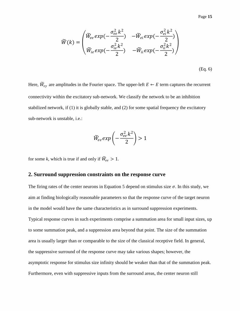
𝑊 (𝑘) =

𝑊 𝑒𝑒𝑒𝑥𝑝(−

𝜍𝑒𝑒2 𝑘2

2) −𝑊 𝑒𝑖𝑒𝑥𝑝(−

𝜍𝑒𝑖2 𝑘2

2)

𝑊 𝑖𝑒𝑒𝑥𝑝(−𝜍𝑖𝑒

2 𝑘2

2) −𝑊 𝑖𝑖𝑒𝑥𝑝(−

𝜍𝑖𝑖2𝑘2

2)

(Eq. 6)

Here, 𝑊 𝑥𝑦 are amplitudes in the Fourier space. The upper-left 𝐸 ← 𝐸 term captures the recurrent

connectivity within the excitatory sub-network. We classify the network to be an inhibition

stabilized network, if (1) it is globally stable, and (2) for some spatial frequency the excitatory

sub-network is unstable, i.e.:

𝑊 𝑒𝑒𝑒𝑥𝑝 −𝜍𝑒𝑒

2 𝑘2

2 > 1

for some k, which is true if and only if 𝑊 𝑒𝑒 > 1.

2. Surround suppression constraints on the response curve

The firing rates of the center neurons in Equation 5 depend on stimulus size 𝜍. In this study, we

aim at finding biologically reasonable parameters so that the response curve of the target neuron

in the model would have the same characteristics as in surround suppression experiments.

Typical response curves in such experiments comprise a summation area for small input sizes, up

to some summation peak, and a suppression area beyond that point. The size of the summation

area is usually larger than or comparable to the size of the classical receptive field. In general,

the suppressive surround of the response curve may take various shapes; however, the

asymptotic response for stimulus size infinity should be weaker than that of the summation peak.

Furthermore, even with suppressive inputs from the surround areas, the center neuron still

receives considerable amount of feed-forward inputs; and the response to stimuli covering the

suppressive surround is still stronger than baseline activity with no stimulus at all (the baseline

activity is zero in our linear model).

Thus we generalize the surround suppression constraints on the response curve as follow:

A. Suppressive surround: we require that the response curves 𝐸(𝑥 = 0, 𝜍)𝐼(𝑥 = 0, 𝜍)

of the neurons at

the center of the stimulus to show a global peak at 𝜍𝑅 , i.e. the maximal response stimulus size,

and 0 < 𝜍𝑅 < ∞. We generally consider stimulus size 𝜍 < 𝜍𝑅 to be in the summation region of

the response curve, and stimulus size 𝜍 > 𝜍𝑅 to be in the suppressive surround, regardless of the

specific shape of the response curve.

B. Non-negative response: surround suppression reduces the firing rate but does not drive the

network below its baseline activity (the spontaneous firing rate). Thus we require that

𝐸(𝑥 = 0, 𝜍)𝐼(𝑥 = 0, 𝜍)

> 0 for all stimulus sizes 𝜍.

C. Stability: the network dynamics given by Equation 2 must be stable. Therefore, in the Fourier

space, all eigenvalues of the connectivity matrix 𝑊 (𝑘) − 𝐼 must have negative real part for all

k. For any 2-by-2 matrix at a given 𝑘 (Equation 6), this means the determinant of the

connectivity matrix is positive while the trace is negative.

In many experiments, the response in the summation center increases monotonically with the

stimulus size; and for stimuli large enough, the response monotonically decreases with the

stimulus size (DeAngelis et al., 1994; Sengpiel et al., 1997; Akasaki et al., 2002; Angelucci et al.,

2002; Ozeki et al., 2004). In the numerical studies (Section 4 to 8 of this chapter), we search for

general cases without the constraint of monotonically decreasing response curve, i.e. solutions

with oscillations in the response curve are allowed. For simplicity, we assume this additional

constraint in the analytic studies (Section 3). Thus, Constraint A can be reduced to analytic

boundary conditions:

A'. Summation for small stimulus: the response curve increases with the stimulus size when

the stimulus size is small:

𝑑

𝑑𝜍 𝐸(0, 𝜍 → 0)𝐼(0, 𝜍 → 0)

> 0

A''. Monotonic suppression for large stimulus: the response curve decreases for stimuli large

enough:

𝑑

𝑑𝜍 𝐸(0, 𝜍 → ∞)𝐼(0, 𝜍 → ∞)

< 0

Under these conditions, the response curve has a single global peak stimulus size 𝜍𝑅 . For

stimulus smaller than 𝜍𝑅 , the response is always non-negative. For stimulus larger than 𝜍𝑅 , as

long as the asymptotic response at stimulus size infinity is non-negative, all responses in the

suppressive surround stay above the activity baseline. This leads to a simplified boundary

condition for non-negative response:

B'. Non-negative response for large stimulus:

𝐸(0, 𝜍 → ∞. )𝐼(0, 𝜍 → ∞. )

> 0

3. Analytic solutions with surround suppression boundary conditions

With Gaussian input functions, we are able to obtain analytic solutions for the model in Section 1,

with the boundary conditions listed in the previous section. The detailed derivations are shown in

Appendix B Section 2c. The results are conditions on the model parameters as follow, equivalent

to the constraints in the previous section:

Solutions under Constraint A':

𝑑𝑘 𝐼 − 𝑊 𝑘 −1

− 𝐼 𝐶𝑒𝐶𝑖

∞

−∞

> 0

Solutions under Constraint A'':

1 + 𝑊 𝑖𝑖 −𝑊 𝑒𝑖

𝑊 𝑖𝑒 1 − 𝑊 𝑒𝑒

𝑊 𝑒𝑒𝜍𝑒𝑒

2 −𝑊 𝑒𝑖𝜍𝑒𝑖2

𝑊 𝑖𝑒𝜍𝑖𝑒2 −𝑊 𝑖𝑖𝜍𝑖𝑖

2 1 + 𝑊 𝑖𝑖 −𝑊 𝑒𝑖


𝐶𝑒𝐶𝑖

< 0

Solutions under Constraint B':



𝐶𝑒𝐶𝑖

> 0

Solutions under Constraint C:

𝐷𝑒𝑡 𝑊 𝑘 − 𝐼 > 0 and 𝑇𝑟 𝑊 𝑘 − 𝐼 < 0, for every 𝑘.

Combining the 𝜍 → ∞ results in A'' and B', we have:

𝑑

𝑑𝜍 𝐸 0, 𝜍 → ∞

𝐼 0, 𝜍 → ∞ =






2 𝐸 0, 𝜍 → ∞

𝐼 0, 𝜍 → ∞ < 0

For the inhibitory neuron at the center of the stimulus:

𝜍𝑒𝑒2 −

𝑊 𝑒𝑒 − 1

𝑊 𝑒𝑒

𝜍𝑖𝑒2 𝐸 0, 𝜍 → ∞ −

𝑊 𝑒𝑖

𝑊 𝑒𝑒

𝜍𝑒𝑖2 −

𝑊 𝑒𝑒 − 1 𝑊 𝑖𝑖

𝑊 𝑒𝑒𝑊 𝑖𝑒

𝜍𝑖𝑖2 𝐼 0, 𝜍 → ∞ < 0

(Eq. 7)

In general, the inhibitory connections are shorter in range compared to the excitatory connections

(Gilbert and Wiesel, 1983; Das and Gilbert, 1995). Excitatory neurons can form long-range

lateral connections (Kisvarday et al., 1997; Azouz et al., 1997, Sceniak et al., 2001, Stettler et al.,

2002) while inhibitory neurons lack such long-range connections. In addition, Equation 7

depends on the square of connection widths. When the inhibitory connections are local, the

contribution of inhibitory term becomes insignificant compared to that of the excitatory term.

Therefore, we immediately have 𝑊 𝑒𝑒 > 1, and the network functions in the ISN regime. In

addition, we also have:

𝜍𝑖𝑒

𝜍𝑒𝑒

2

>𝑊 𝑒𝑒

𝑊 𝑒𝑒 − 1> 1

Thus 𝜍𝑖𝑒 > 𝜍𝑒𝑒 , which means the 𝐼 ← 𝐸 connections are longer in range than the 𝐸 ← 𝐸

connections.

4. General numerical solutions with parameter space search

In this section we obtain numerical solutions given by the Constraints A, B and C in Section 2

without simplifications or approximations for the analytic solutions. The width of 𝐸 ← 𝐸

connection is set to be the unit length 𝜍𝑒𝑒 ≡ 1; and there are 9 free parameters in the model: the

widths of the connections: 𝜍𝑒𝑖 , 𝜍𝑖𝑒 , 𝜍𝑖𝑖 ; the amplitudes of the connections: 𝑊𝑒𝑒 , 𝑊𝑒𝑖 , 𝑊𝑖𝑒 , 𝑊𝑖𝑖 ; the

width of the input blurring 𝜍0; and the ratio of the intensities of the input to the excitatory and the

inhibitory neurons: 𝑐𝑒/𝑐𝑖. We perform an exhaustive parameter space search and check the

resulting response curves against the surround suppression constraints. The parameter space is

chosen to have a wide range, covering biologically reasonable cases, but we do not restrict the

parameter space specifically to contain only biologically reasonable solutions. The 𝐼 ← 𝐸

connection width is chosen to be comparable to 𝐸 ← 𝐸 connection width, up to about twice as

wide: 𝜍𝑖𝑒 = (0.7, 0.9, 1.1, 1.3, 1.5, 1.7, 1.9). In general, inhibitory connections are shorter ranged

than the excitatory connections: 𝜍𝑒𝑖 , 𝜍𝑖𝑖 = (0.05, 0.1, 0.3, 0.5, 0.7, 0.9, 1.3), we include 𝜍𝑒𝑖 , 𝜍𝑖𝑖 =

0.05 to account for local inhibitory connection. Although biologically unlikely, we also allow

𝜍𝑒𝑖 , 𝜍𝑖𝑖 = 1.3 so that we do not exclude the possibility of long range inhibitory connections. The

amplitudes of excitatory connections are given by 𝑊𝑒𝑒 , 𝑊𝑖𝑒 = (0.20, 0.35, 0.50, 0.65, 0.80).

Since 𝜍𝑒𝑒 = 1 and 𝑊 𝑒𝑒 = 2𝜋𝑊𝑒𝑒𝜍𝑒𝑒 , both non-ISN (𝑊 𝑒𝑒 < 1) and ISN (𝑊 𝑒𝑒 > 1) solutions are

possible in the simulation. The amplitudes of inhibitory connections have a wide range:

𝑊𝑒𝑖 , 𝑊𝑖𝑖 = (0.1, 0.2, 0.4, 0.8, 1.6, 3.2, 6.4), so that in the local inhibitory connection case, the

area under the envelope of the inhibitory Gaussian weight functions (given by 𝑊𝑒𝑖𝜍𝑒𝑖 and 𝑊𝑖𝑖𝜍𝑖𝑖 )

could still be comparable to that of the excitatory ones. The width of the blurring 𝜍0 ranges up to

the width of the 𝐸 ← 𝐸 connection: 𝜍0 = (0.0, 0.25, 0.5, 1.0). The ratio of the inputs to

excitatory vs. inhibitory neurons is: 𝑐𝑒/𝑐𝑖 = (0.5, 1.0, 2.0). For each parameter combination, the

stability of the network is checked first. Then for the stable networks, the response curve is

computed numerically and checked against Constraint A and B. Numerical results are obtained

for both Gaussian and Rectangular input functions.

We first compare the numerical results to the analytic results with local inhibition in the previous

section. We set the inhibition width to be short ranged: 𝜍𝑒𝑖 , 𝜍𝑖𝑖 = 0.05. Since the previous

analytic result suggested long range 𝐼 ← 𝐸 connection (𝜍𝑖𝑒 > 𝜍𝑒𝑒 ), the range of 𝜍𝑖𝑒 is extended

to up to about 4.0 for better illustration. The ranges of the other parameters remain unchanged.

Figure 4a is an example with Gaussian input function, 𝑐𝑒/𝑐𝑖 = 1.0 and no blurring 𝜍0 = 0. The

numerical results agree with analytic ones: all solutions are in the ISN regime (𝑊 𝑒𝑒 > 1) with

long range 𝐼 ← 𝐸 connection (𝜍𝑖𝑒 > 𝜍𝑒𝑒 ).

Next, we examine the general numerical solutions over the entire parameter space. To simplify

the illustration, we first plot the results in the density maps of the connection widths 𝜍𝑖𝑒 , 𝜍𝑒𝑖 and

𝜍𝑖𝑖 in the 3-dimensional 𝜍 subspace. Figure 4b is an example with Gaussian input function,

𝑐𝑒/𝑐𝑖 = 1.0 and 𝜍0 = 0, color coded by solution density. The solution density increases as 𝜍𝑖𝑒 and

𝜍𝑒𝑖 become larger.

For each solution in the parameter space, we quantify the strength of surround suppression by

calculating the Suppression Index (𝑆𝐼), defined as the ratio of the peak-to-infinity suppression vs.

the peak response:

𝑆𝐼 =𝑅𝑒𝑠𝑝𝑜𝑛𝑠𝑒𝜍𝑅

− 𝑅𝑒𝑠𝑝𝑜𝑛𝑠𝑒𝜍→∞

𝑅𝑒𝑠𝑝𝑜𝑛𝑠𝑒𝜍𝑅

where 𝜍𝑅 is the stimulus size at maximal response. The suppression indices are calculated for the

excitatory and the inhibitory populations respectively (𝑆𝐼𝑒 , 𝑆𝐼𝑖). When used without sub-indices,

𝑆𝐼 is the minimum of 𝑆𝐼𝑒 and 𝑆𝐼𝑖 . We consider solutions with 𝑆𝐼 < 5% to be insignificantly

surround-suppressed and solutions with 𝑆𝐼 ≥ 50% to be strongly surround-suppressed. Figure 4c

and 4d are density maps of the 3-dimensional 𝜍 subspace, color coded by the averaged 𝑆𝐼 of the

excitatory and the inhibitory responses respectively. In general, excitatory response curves show

stronger surround suppression compared to the inhibitory ones (different levels in color coding

legend), and solutions with strong surround suppression tend to cluster in the region with large

𝜍𝑖𝑒 and 𝜍𝑒𝑖 .

In Figure 4b-4d, the solution density only weakly depends on the width of the 𝐼 ← 𝐼 connection

𝜍𝑖𝑖 . Thus we project the 3-D map on the 𝜍𝑖𝑒 vs. 𝜍𝑒𝑖 plane, as shown in Figure 4e. Excitatory

neurons can effectively inhibit neighboring excitatory neurons via an 𝐸 ← 𝐼 ← 𝐸 connection

chain, where each excitatory neuron projects to its neighboring inhibitory neurons and the

inhibitory neurons further suppress their neighboring excitatory neurons. The width of such

lateral inhibition is 𝜍𝑒𝑖2 + 𝜍𝑖𝑒

2 :

𝑑𝑥′ exp − 𝑥 − 𝑥 ′ 2

2𝜍𝑒𝑖2 exp −

𝑥′2

2𝜍𝑖𝑒2 ∝ exp −

𝑥2

2 𝜍𝑒𝑖2 + 𝜍𝑖𝑒

2

(Eq. 8)

The solid curve in Figure 4e represents 𝜍𝑒𝑖2 + 𝜍𝑖𝑒

2 = 𝜍𝑒𝑒2 = 1; all solutions are above this curve,

i.e. the lateral inhibition has longer range compared to the lateral excitation by 𝐸 ← 𝐸 connection.

The region above the broken line is given by the biological constraint 𝜍𝑖𝑒 > 𝜍𝑒𝑖 . Within this

region, all solutions satisfy 𝜍𝑖𝑒 > 𝜍𝑒𝑒 , i.e. the 𝐼 ← 𝐸 projection is wider than the 𝐸 ← 𝐸

projection. In general, surround suppression solutions favor large 𝜍𝑖𝑒 ; separate search results

with wider range of 𝜍𝑖𝑒 show that surround suppression solutions are abundant when 𝜍𝑖𝑒 > 2𝜍𝑒𝑒 .

Next, we examine the connections amplitudes in the Fourier space: 𝑊 𝑒𝑒 , 𝑊 𝑒𝑖 , 𝑊 𝑖𝑒 and 𝑊 𝑖𝑖 . To

illustrate the results in a 3-dimentional map, we normalize all amplitudes by the amplitude of the

𝐸 ← 𝐸 connection. Figure 5a is the 3-dimensional map of the relative amplitudes in Fourier

space: 𝑊 𝑒𝑖 /𝑊 𝑒𝑒 , 𝑊 𝑖𝑒 /𝑊 𝑒𝑒 and 𝑊 𝑖𝑖/𝑊 𝑒𝑒 , color coded by solution density. Figure 5b and 5c are the

same map color coded by suppression index of excitatory and inhibitory responses respectively.

The plane in Figure 5a is a least squares fit of the data, given by 𝑊 𝑒𝑒 = 2.10𝑊 𝑒𝑖 + 0.35𝑊 𝑖𝑒 −

1.21𝑊 𝑖𝑖 .

The amplitude of the 𝐸 ← 𝐸 connection 𝑊 𝑒𝑒 determines whether the network is an ISN or not.

Figure 6 is the histogram of 𝑊 𝑒𝑒 , grouped and color coded by the minimal suppression index 𝑆𝐼.

Most solutions are in the ISN regime, more than 88% of all solutions have 𝑊 𝑒𝑒 > 1, and most of

the non-ISN solutions only show insignificant surround suppression (𝑆𝐼 < 5%). Apart from such

solutions, only less than 1% of the total solutions are non-ISN. Stronger surround suppression

favors large amplitude of the 𝐸 ← 𝐸 connection. For groups with 𝑆𝐼 ≥ 10%, most solutions have

very strong recurrent connections in the excitatory sub-network, i.e. 𝑊 𝑒𝑒 ≥ 1.625.

5. Amplification at critical filter frequency

The stability of the weight matrix 𝑊 is checked for all spatial frequencies. The stability of 𝑊 (𝑘)

at a given spatial frequency 𝑘 is determined by the largest real parts of all eigenvalues of 𝑊 (𝑘).

We define the eigenvalue with the largest real part across all spatial frequencies to be the 'leading

eigenvalue'. Figure 7 is the histogram of the real part of this leading eigenvalue of 𝑊 (𝑘) for all

numerical solutions, color coded by the suppression index. Networks with strong surround

suppression (𝑆𝐼 ≥ 50%) are generally closer to instability, as the real part of the leading

eigenvalue is close to 1. We define the critical filter frequency 𝑘𝐹 to be the frequency

corresponding to the leading eigenvalue of the inverse of the connectivity matrix 𝐼 − 𝑊 (𝑘) −1

.

From a signal processing point of view, the neuronal response in Equation 5 is the result of the

input signal 𝑕 𝑒(𝑘)

𝑕 𝑖(𝑘) passing through the band-pass filter 𝐼 − 𝑊 (𝑘)

−1. When the network

approaches instability, 𝐷𝑒𝑡 𝐼 − 𝑊 𝑘𝐹 → 0, and the inverse of the connectivity matrix

𝐼 − 𝑊 (𝑘) −1

has a sharp peak around 𝑘𝐹 , providing a large amplification for inputs with

frequencies comparable to 𝑘𝐹 .

We expand the filter 𝐼 − 𝑊 (𝑘) −1

as a series in 𝐷𝑒𝑡 𝐼 − 𝑊 𝑘 ; dropping the higher order

terms (See Appendix B Section 2d for details), we arrive at:

𝐼 − 𝑊 𝑘 −1

~1

𝐷𝑒𝑡 𝐼 − 𝑊 𝑘

1 + 𝑊 𝑖𝑖 𝑘

𝑊 𝑖𝑒 𝑘 1 + 𝑊 𝑖𝑖 𝑘 −𝑊 𝑒𝑖 𝑘

(Eq. 9)

In Equation 9, the filter acts as a projection operator, mapping the input vector 1 + 𝑊 𝑖𝑖 𝑘

−𝑊 𝑒𝑖 𝑘

into the output vector 1 + 𝑊 𝑖𝑖 𝑘

𝑊 𝑖𝑒 𝑘 . For Gaussian input functions, the input at frequency 𝑘𝐹 is

𝑕 𝑒(𝜍, 𝑘𝐹)

𝑕 𝑖(𝜍, 𝑘𝐹) = 2𝜋𝜍𝑒−𝑘𝐹

2 𝜍2+𝜍02

2 𝑐𝑒

𝑐𝑖 , which reaches its maximum at the critical stimulus

size 𝜍𝐹 ≡ 1/𝑘𝐹, as illustrated in Figure 8 top panel. As long as the stimulus is not orthogonal to

the input vector, i.e. 1 + 𝑊 𝑖𝑖(𝑘) −𝑊 𝑒𝑖 (𝑘) 𝑐𝑒

𝑐𝑖 ≠ 0, the response curve would reach its peak

around the critical stimulus size, as illustrated in Figure 8 bottom panel: 𝜍𝑅~𝜍𝐹, where 𝜍𝑅 is the

maximal response stimulus size. In addition, for solutions with strong surround suppression

(𝑆𝐼 ≥ 50%), the response at critical stimulus size 𝐸 0, 𝜍𝐹

𝐼 0, 𝜍𝐹 should be linearly dependent on

the filter output vector 1 + 𝑊 𝑖𝑖 𝑘𝐹

𝑊 𝑖𝑒 𝑘𝐹 around the critical filter frequency 𝑘𝐹 . Figure 9a shows

the ratio of the responses at the critical stimulus size 𝐸 0, 𝜍𝐹 /𝐼 0, 𝜍𝐹 vs. the ratio of the

output vector 1 + 𝑊 𝑖𝑖 𝑘𝐹 /𝑊 𝑖𝑒 𝑘𝐹 for all solutions with 𝑆𝐼 ≥ 50% (286 solutions). The

result shows a linear dependency: the solid line is the linear least squares fit, given by 𝐸/𝐼 =

0.87 1 + 𝑊 𝑖𝑖 /𝑊 𝑖𝑒 − 0.08, 𝑟2 = 0.94.

A saddle point approximation around the critical filter frequency 𝑘𝐹 show that, for solutions with

weaker surround suppression, the maximal response stimulus size 𝜍𝑅 is generally larger than the

critical stimulus size 𝜍𝐹 (the mathematical details are given in Appendix B, Section 2e). Figure

9b is the scatter plot of the maximal response stimulus size 𝜍𝑅 vs. the critical stimulus size 𝜍𝐹 for

all solutions. In general, most solutions satisfy 𝜍𝑅 ≥ 𝜍𝐹; and for solutions with strong surround

suppression (𝑆𝐼 ≥ 50%.), 𝜍𝑅 is very close to 𝜍𝐹 .

6. Strong surround suppression generated by stable sparse networks

In the above section, networks with strong surround suppression tend to approach instability. To

improve stability, we introduce random sparseness to the connectivity matrix; and across several

random instantiations, we choose the ones whose real part of the leading eigenvalue is smaller

than that of the original dense matrix. Despite this reduction in eigenvalue, some neurons in

these sparse networks show very strong surround suppression effects.

Sparseness in the connections is modeled in the weight matrix as a form of variability, while the

overall envelope of connectivity functions remains unchanged. We simulate networks of 4000

neurons (2000 excitatory and 2000 inhibitory) with densely connected matrices given by

different parameters in Section 4. We randomly set the weights in the 'dense' matrix to 0 with

probability 1 − 𝑠, where 𝑠 is the sparseness factor (𝑠 = 5%, 10%, 20%). The resulting sparse

matrix is normalized so that the sum of the excitatory weights and the sum of the inhibitory

weights to each cell remain the same as the dense matrix. In the previous sections, the weight

matrix was translation-invariant; therefore all neurons had the same response curve and 𝑆𝐼 value.

Sparseness breaks the translation-invariance, and neurons in the sparse network have different

responses curves and 𝑆𝐼 values.

Figure 10a shows the population distribution of the 𝑆𝐼 values in two different scenarios where

the population 𝑆𝐼 values of the dense matrices are at different levels. Population 1 corresponds to

a case of low population 𝑆𝐼 in the dense matrix, where the averaged population suppression

indices are 𝑆𝐼𝑒 = 33% and 𝑆𝐼𝑖 = 21%, for the excitatory and the inhibitory sub-populations. The

simulation parameters are: 𝜍𝑒𝑖 = 0.5, 𝜍𝑖𝑒 = 1.9, 𝜍𝑖𝑖 = 0.3, 𝑊𝑒𝑒 = 0.65, 𝑊𝑒𝑖 = 0.4, 𝑊𝑖𝑒 = 0.5,

𝑊𝑖𝑖 = 0.4, 𝑐𝑒/𝑐𝑖 = 1.0, 𝜍0 = 0 and 𝑠 = 20%. The distribution is unimodal, similar to the

experimental results reported by Walker et al (Walker et al., 2000). Population 2 is another

sparse network with stronger surround suppression in the dense matrix (𝑆𝐼𝑒 = 58% and 𝑆𝐼𝑖 =

48%), simulation parameters: 𝜍𝑒𝑖 = 0.5, 𝜍𝑖𝑒 = 1.9, 𝜍𝑖𝑖 = 0.3, 𝑊𝑒𝑒 = 0.8, 𝑊𝑒𝑖 = 0.8, 𝑊𝑖𝑒 =

0.5, 𝑊𝑖𝑖 = 0.4, 𝑐𝑒/𝑐𝑖 = 1.0, 𝜍0 = 0 and 𝑠 = 20%. The distribution is bimodal, similar to the

experimental results with a heavy tail at high 𝑆𝐼 values (Jones et al., 2000; Akasaki et al., 2002).

Neither sparse matrix is close to instability, since the real parts of their leading eigenvalues

satisfy 𝑟𝑒𝑎𝑙 𝜆𝐿 < 0.9. Nonetheless, both examples contain neurons with very strong surround

suppression (𝑆𝐼 ≥ 90%). In contrast, when the same sparseness is introduced to dense networks

with insignificant 𝑆𝐼 values (𝑆𝐼 = 2%, for population 3 and population 4), all neurons in the

sparse network have low 𝑆𝐼 values even when the network approaches instability, i.e. the real

part of the leading eigenvalues is very close to 1: 𝑟𝑒𝑎𝑙 𝜆𝐿 > 0.95 (Figure 10b).

7. Effects of different input functions with different blurring widths

The previous sections focused on the results with Gaussian input function without blurring

(𝜍0 = 0). In this section, we examine surround suppression effects under different stimulus

conditions: two types of input functions (Gaussian or Rectangular) with three different blurring

widths: 𝜍0 = (0.25, 0.5, 1.0).

Figure 11 shows an example of the results with input blurring, where the input function is

Gaussian and the blurring width 𝜍0 = 0.25. The input blurring increases the number of solutions

(22268 solutions in the blurring result vs. 7199 in the non-blurring result). Figure 11a, 11b and

11c show the input blurring solutions in the 𝜍 subspace and 𝑊 subspace. These new solutions

have a similar structure in the 𝜍 subspace compared to the solutions without input blurring. In

the 𝑊 subspace, the solutions cover a larger range along each axis. The red markers in Figure

11c represent solutions that also appear in the results without blurring. Such solutions tend to

cluster in the local inhibition region where both 𝐼 ← 𝐸 and 𝐼 ← 𝐼 connections are short in range.

In results with no input blurring, solutions with strong surround suppression were characterized

by the critical filter frequency 𝑘𝐹 , and 𝜍𝑅~𝜍𝐹, as shown in Figure 9b. In Figure 11d, solutions

with input blurring are plotted in the same way, color coded by the suppression index. Here,

solutions with strong surround suppression (dark red) can be roughly divided into two clusters.

The first cluster along the diagonal of 𝜍𝑅 = 𝜍𝐹 corresponds to the solutions obtained without

input blurring. The second cluster contains solutions whose maximal response stimulus size 𝜍𝑅 is

small and is independent of the critical stimulus size 𝜍𝐹 .

The second cluster of solutions represents networks where the recurrent input to the central

neuron is globally inhibitory. Such networks generate monotonically decreasing response curves

in the absence of input blurring. With input blurring, the feed-forward input received by the

center neuron is the stimulus convolved with the blurring function. When the stimulus size is

much smaller than the width of the input blurring, the convolution is roughly proportional to the

sum of the stimulus over positions. Thus, the response curves of the center neurons always show

an initial summation. When the stimulus size becomes larger, this feed-forward summation effect

becomes weaker than the recurrent inhibition effect; and the response becomes surround-

suppressed. In these networks, the initial summation is short in range compared to the width of

𝐸 ← 𝐸 connection (𝜍𝑒𝑒 = 1).

Figure 12 shows the results with Rectangular functions without input blurring. There are more

solutions (84487 solutions) than that of the Gaussian input functions (7199 solutions). These

solutions span the entire 𝜍 subspace, as shown in Figure 12a and 12b. Most of the new solutions

have very small 𝜍𝑒𝑖 (Figure 12c top panel). Such solutions generate monotonically increasing

response curves with Gaussian input functions, i.e. the maximum of the response curve is at

𝜍 → ∞ . At 𝜍 → ∞ the population response depends on the inverse Fourier transform of the

input function (Appendix B, Section 2c), hence the response of the center neuron (𝑥 = 0) is

given by the integral 𝑕 (𝑘)∞

−∞𝑑𝑘. The Fourier transform of a Rectangular function is the Sinc

function. The area under the central peak of the Sinc function ([−1/𝜍, 1/𝜍]) is larger than the

entire integral over the real line:

𝑠𝑖𝑛𝜋𝜍𝑘

𝜋𝜍𝑘

1/𝜍

−1/𝜍

𝑑𝑘~1.18 𝑠𝑖𝑛𝜋𝜍𝑘

𝜋𝜍𝑘

∞

−∞

𝑑𝑘

Most of these solutions do not show resonance in the connectivity filter as describe in Section 5,

and their connectivity filters peak at 𝑘 = 0. Thus, a global peak in the response curve may

appear when the central peak of the Sinc function is optimal for the connectivity filter, and such

solutions become surround suppression solutions as defined in Constraint A, Section 2.

Most of these new solutions have very insignificant surround suppression (𝑆𝐼 < 1%); and the

solutions with significant surround suppression (𝑆𝐼 ≥ 5%) satisfy 𝜍𝑒𝑖2 + 𝜍𝑖𝑒

2 > 𝜍𝑒𝑒2 = 1 (Figure

12c bottom panel), similar to the results with Gaussian input functions. Such similarities in

distribution are also seen in the 𝑊 subspace (Figure 12d and 12e), for solutions with large 𝑆𝐼.

8. Spatial oscillations in population activity

As mentioned in Section 5, many surround suppression solutions (especially the ones with very

strong 𝑆𝐼) have a sharp peak in the filter 𝐼 − 𝑊 (𝑘) −1

around the critical frequency 𝑘𝐹 . Figure

13a shows the histograms of the critical frequency 𝑘𝐹 for solutions with Gaussian input and no

blurring. The top panel contains all 7199 solutions with 𝑆𝐼 > 0% and most solutions have

𝑘𝐹 > 0 (7161 out of 7199). The bottom panel shows solutions with 𝑆𝐼 ≥ 50% (286 solutions),

and all solutions have 𝑘𝐹 > 0. The population activity is given by the inverse Fourier transform

of the filtered input in the Fourier space (Equation S7, Appendix B, Section 2a). Therefore, the

sharp peak at 𝑘𝐹 > 0 in the filter 𝐼 − 𝑊 (𝑘) −1

can lead to spatial oscillations in the population

activity. Figure 13b illustrates population activity patterns of an example network at various

stimulus sizes (network parameters: 𝜍𝑒𝑖 = 0.5, 𝜍𝑖𝑒 = 1.9, 𝜍𝑖𝑖 = 0.3, 𝑊𝑒𝑒 = 0.65, 𝑊𝑒𝑖 = 0.4,

𝑊𝑖𝑒 = 0.5, 𝑊𝑖𝑖 = 0.4, same as Population 1 in Section 6), and the critical stimulus size is

𝜍𝐹 = 1.1. When the stimulus size is small, the population response is localized around 𝑥 = 0. As

the stimulus size increases, a population oscillation emerges and becomes strong when the

stimulus size is comparable to the critical stimulus size. When the stimulus size becomes very

large, the population response becomes constant and the oscillation disappears.

For Gaussian input functions, there is one global critical stimulus size 𝜍𝐹 corresponding to the

resonant frequency 𝑘𝐹 , as illustrated in Figure 8 top panel. The response curve of the center

neuron has a single peak at 𝜍𝑅~𝜍𝐹, as shown in Figure 8 bottom panel. But for a Rectangular

input function, the Fourier transform is a Sinc function with multiple peaks and troughs. Each

time a peak matches the critical frequency 𝑘𝐹 in the Fourier space, the corresponding response

curve of the neuron at the center will have a local maximum at 𝜍𝑅~𝜍𝐹; i.e. the response curve

oscillates with stimulus size. Such oscillations were reported in previous experiments (Sengpiel

et al., 1997; Anderson et al., 2001). The population activity will also oscillate as a result of

resonance. When a peak of the input matches the critical frequency 𝑘𝐹 in the Fourier space, the

population activity peaks at the center neuron. In contrast, when a trough of the input matches

the critical frequency 𝑘𝐹 , the center neuron corresponds to a trough in population activity.

Therefore, as the input size increases, the network repeatedly gains and loses resonance; and the

population activity will alternate between oscillatory and non-oscillatory states.

9. Summary

In this chapter, we studied a linear rate model for both excitatory and inhibitory neuronal

populations of a single preferred orientation, with a connectivity matrix dependent on the relative

position of the neurons. We searched for conditions when the connectivity functions produced

surround suppression in both excitatory and inhibitory neurons at the center of the stimulus. For

Gaussian input functions, we obtained analytic solutions with surround suppression boundary

conditions simplified from general surround suppression constraints. In addition, if the inhibitory

connections were short ranged, in order for the inhibitory response to decrease with increasing

stimulus size, two conditions must be met: (1) the network must be an ISN; and (2) the 𝐼 ← 𝐸

connections must be longer-ranged than the 𝐸 ← 𝐸 connections.

We performed an exhaustive parameter space search to obtain general numerical solutions

without additional simplifications and approximations. The numerical solutions verified the

findings in the analytic results. We calculated the suppression index to characterize the strength

of the surround suppression for each numerical solution. Excluding solutions with insignificant

surround suppression (𝑆𝐼 < 5%), there were two key factors for a network to generate

significant surround suppression: (1) strong recurrence in the 𝐸 ← 𝐸 sub-network (𝑊 𝑒𝑒 > 1, ISN

regime) and (2) wider 𝐼 ← 𝐸 connection width than 𝐸 ← 𝐸 connection width. In general, many

networks with 𝑊 𝑒𝑒 > 1.5 and 𝜍𝑖𝑒 > 2𝜍𝑒𝑒 showed surround suppression effects as long as the

network is overall stable.

Networks with strong surround suppression (𝑆𝐼 ≥ 50%) are generally less stable compared to

the ones with weaker 𝑆𝐼 values. When the real parts of the leading eigenvalues of 𝑊 (𝑘)

approaches 1, the corresponding network behaves like a narrow band-pass filter around a critical

filter frequency 𝑘𝐹 . Approximation around this critical filter frequency provides a reasonable

estimate of the maximal responses for solutions with strong surround suppression. We also

predicted that the critical stimulus size 𝜍𝐹 ≡ 1/𝑘𝐹 is generally smaller than the maximal

response stimulus size 𝜍𝑅 .

Next, we introduced variability to the model, allowing sparse connections in the connectivity

matrix (200 to 800 connections per neuron in our simulations, instead of an all-to-all connection).

Depending on the population 𝑆𝐼 of the dense matrix, the 𝑆𝐼 values for individual neurons varied

widely in the sparse network. Neurons with very strong surround suppression were found in such

sparse networks, while such networks generally stayed away from instability. When the dense

network had relatively smaller population 𝑆𝐼, a unimodal distribution of 𝑆𝐼 values was seen in

the sparse network. Furthermore, strong population 𝑆𝐼 in the dense matrix led to a bimodal

distribution of the 𝑆𝐼 values in the sparse network. Both distributions had been reported by

previous experiments. In contrast, if the corresponding dense matrix only produced insignificant

surround suppression (𝑆𝐼 < 5%), the 𝑆𝐼 values of neurons in the sparse network remained small.

We also examined the effect of different input functions and different levels of input blurring. In

the results with Gaussian input functions and no blurring, there is a group of solutions with

strong 𝑆𝐼, whose maximal response stimulus sizes 𝜍𝑅 could be predicted by the critical stimulus

size 𝜍𝐹 . With input blurring, there were more surround suppression solutions in addition to the

ones obtained without input blurring. Among the solutions with strong surround suppression,

there was a new group of solutions corresponding to networks with globally inhibitory recurrent

inputs. In this group, the maximal response stimulus size 𝜍𝑅 was small and was independent of

the critical stimulus size 𝜍𝐹 . Meanwhile, Rectangular input function also increased the number of

surround suppression solutions, and the solutions with strong 𝑆𝐼 had similar distributions in the

parameter space compared to solutions with Gaussian input function.

In general, the response curve given by Equation 5 can also be interpreted from a signal

processing perspective where the input signal passes through the connectivity filter 𝐼 −

𝑊 (𝑘) −1. For solutions with critical frequency 𝑘𝐹 > 0, the population activity in the linear space

may oscillate due to resonance at 𝑘𝐹 . This prediction should be tested by future experiments.

Chapter III: Properties of spontaneous and sensory-driven

activities in the primary visual cortex of awake ferret

1. Experimental procedure and data acquisition

In this chapter we study extra-cellular recordings of awake ferrets (courtesy of Michael Weliky's

lab at University of Rochester). The recordings were gathered from linear arrays of 16 electrodes,

implanted in the primary visual cortex of ferrets. Each electrode array was placed at 300–500μm

depth in layer 2/3 of the primary visual cortex. The entire electrode array spanned 3mm with a

200μm distance between neighboring electrodes, covering a large portion of primary visual

cortex. In most cases, each electrode recorded multi-unit signals from neurons in the proximity.

A moving window average algorithm was used to remove background spiking activity and to

identify the spike trains (see Appendix B, Section 3 for detailed information about the

experimental procedure and data acquisition).

The experiment was performed in awake animals at different developmental stages. After birth,

eyes of the ferrets remained closed until about a month later. The first age group was at postnatal

age P29-P30 (n=3), around eye opening. The second group was at postnatal age P44-P45 (n=3),

during the critical period for ocular dominance plasticity, when orientation tuning and long-range

horizontal connections had developed. The third group of postnatal age P83-P86 (n=4) was the

typical matured age of the animal. A late group, 1 to 3 months after the third age group, was also

included in the experiment at postnatal age P129-P168 (n=6). During the experiment, a given

animal only contributed to the recordings of a single age group.

The experiment also studied the effect of different viewing conditions. Spontaneous activities

were measured under complete darkness. Sensory-driven activities were measured with both a

natural scene movie and a white noise stimulus. The movie stimulus was taken from the movie

'Matrix', and so had spatial and temporal correlations typical of natural vision. Experiments on a

given day of each age group usually contained 15 sessions of 100 seconds recording for each

viewing condition, with the exception of P30a (26 sessions) and P168 (11 sessions). Recordings

of the same viewing condition were done within one recording block, with 5 seconds interval

between successive recording sessions.

2. Principal Component Analysis of the spike trains and the dominance of a

spatially long-ranged principal component

Recordings from the experiments in the previous section are 100 seconds long spike trains. We

received the data as spike counts in 2ms bins. The recording sessions were grouped by postnatal

ages and viewing conditions. Figure 14 shows examples of the spike trains in each age group

with all three viewing conditions. In the matured age groups P83-P86 and P129-P168,

microbursts across all electrodes can be seen in the spike train.

Fiser et al. (2004) previously examined this data, separately studying the spatial correlations and

temporal correlations. They found that: (1) the correspondence between sensory-driven activity

and the structure of the input signal was weak in young animals, but systematically improved

with age; (2) correlations in spontaneous neural firing were only slightly modified by visual

stimulation; and (3) oscillations emerged in the spontaneous activities in the matured age group.

In this study, we examine the spatiotemporal structure of the recordings. We first re-sample the

spike trains into 10ms bins to reduce the number of empty bins. Then we normalize the re-

sampled data so that the recording on each electrode has zero mean and unit variance. To

identify spatially uncorrelated signals, we apply Principal Component Analysis (PCA) to the

normalized data for each recording session, analyzing the set of equal-time spatial vectors in

each 10ms bin, and obtained 16 uncorrelated spatial components. Figure 15a shows an example

of the PCA result from P129, dark viewing condition, session 1. The top panel illustrates the

shape of all 16 principal components, ordered by their contributions to the total variance (shown

in the bottom panel). The 1st principal component (1st PC) is a dominant mode, accounting for

more than 50% of the total variance. This mode is also long-ranged in space, covering the 3mm

span of the electrode array. Other PC modes contribute less to the total variance; and modes with

higher spatial frequencies tend to have less contribution to the variance.

In addition to the principal component analysis, we also examine the overall correlation structure

of the activity pattern by calculating the correlations between spike trains with time lag 𝜏 and

spatial separation 𝑥, i.e. the spatiotemporal cross-covariance matrix:

𝐶 𝑥, 𝜏 =1

𝑁𝑥

1

2𝑖 ,𝑡

𝑆𝑖𝑡𝑆𝑖+𝑥

𝑡+𝜏 + 𝑆𝑖𝑡𝑆𝑖−𝑥

𝑡+𝜏

(Eq. 10)

where 𝑆 is the normalized spike train, 𝑖 is the index of the electrode, and 𝑁𝑥 is a normalizing

factor (the number of electrode pairs separated by distance 𝑥). In Figure 15b, the top panel is the

cross-covariance matrix calculated for P129, dark viewing condition, session 1. The

characteristic structure is approximately a spatially homogeneous mode spanning across all

electrodes, with a damped oscillation along the temporal axis. In the bottom panel, the

contribution of the1st PC mode is removed from the spike train, and the resulting plot only

contains the contributions from the other PC modes. In this plot, structure of the 𝐶 𝑥, 𝜏 is

characterized by a short-lived sharp peak around 𝜏 = 0 and 𝑥 = 0, and all correlations quickly

decay to background level in about 50ms.

This spatially homogeneous 1st PC mode is a dominant component in all age groups, as shown

in Figure 15c, where recordings from the same age group are pooled together. The top panel

illustrates the averaged 1st PC mode in each age group, which resembles a spatial DC mode (the

dotted line: 0.25 on each of the 16 electrodes, i.e. a DC vector of unit length). The bottom panel

shows the percentage of the total variance of each corresponding PC mode, similar to the bottom

panel in Figure 15a. Table 1 below lists the absolute value of the difference between the 1st PC

mode and the DC mode on each electrode (normalized by the DC mode and then averaged over

all electrodes) and the percentage contribution of the 1st PC mode to the total variance:

Table 1

Age Group P29-P30 P44-P45 P83-P86 P129-P168

Difference (mean ± sem) 12% ± 2% 17% ± 4% 9% ± 2% 6% ± 1%

% of Variance (mean ± sem) 22% ± 2% 23% ± 1% 38% ± 4% 42% ± 2%

In all age groups, the 1st PC mode represents a spatially long-ranged component in the activity

pattern. Especially in the late age group (P129-P168), this mode is essentially a spatial DC mode.

The 1st PC also carries a bigger percentage of the total variance in matured age groups.

We compare the auto-covariance curves of all PC modes and search for differences in their

temporal correlation structures. The 1st PC mode is a slow component for all age groups. As the

animal matures, the temporal correlations decay at a faster rate in all PC modes. However, the

reduction in temporal correlation is less in the 1st PC mode than in the other PC modes. Figure

15d shows the auto-covariance of the top four PC modes for age group P83-P86 (top panel) and

P129-P168 (bottom panel). The results are averaged across all recording days and all sessions for

a given age group. The 1st PC mode is a slow temporal mode, typically lasting for several

hundred milliseconds in the auto-covariance curve. Other PC modes decay into baseline level

much more quickly in matured age groups. We calculate the baseline correlation by averaging

the auto-covariance at large 𝜏 (2s~5s) for each PC mode in each session. We define the

characteristic decay time of each PC mode to be the first time when the temporal correlation falls

within 2 standard error of the mean from the baseline level. The results of the spontaneous

activities are detailed in Table 2 (mean ± sem, averaged within each age group, unit in ms). The

results under movie and noise viewing conditions can be found in Supplemental Table 1 and 2,

Appendix B Section 4a.

Table 2


PC 1 907 ± 218 433 ± 258 253 ± 92 318 ± 27

PC 2 743 ± 203 373 ± 303 50 ± 7 58 ± 14

PC 3 793 ± 519 310 ± 235 40 ± 9 68 ± 32

PC 4 453 ± 179 237 ± 79 45 ± 12 55 ± 14

PC 5 437 ± 252 193 ± 113 48 ± 18 30 ± 6

PC 6 280 ± 135 153 ± 84 48 ± 9 37 ± 3

PC 7 343 ± 181 177 ± 215 38 ± 12 38 ± 5

PC 8 343 ± 170 193 ± 118 38 ± 11 38 ± 9

PC 9 290 ± 142 190 ± 125 45 ± 12 38 ± 5

PC 10 293 ± 205 190 ± 130 35 ± 13 37 ± 4

PC 11 333 ± 189 167 ± 122 33 ± 13 38 ± 7

PC 12 270 ± 155 120 ± 60 35 ± 13 33 ± 11

PC 13 210 ± 162 67 ± 3 33 ± 13 28 ± 5

PC 14 193 ± 141 63 ± 9 38 ± 14 28 ± 7

PC 15 147 ± 99 63 ± 3 35 ± 13 25 ± 3

PC 16 90 ± 70 50 ± 12 30 ± 9 27 ± 3

In general, PC modes with less contribution to the total variance tend to decay faster. In the

matured age groups P83-P86 and P129-P168, the 1st PC mode has significantly larger

characteristic decay time than the other PC modes. The characteristic decay time of the 1st PC

mode is about 5 to 10 times bigger than the largest characteristic decay time of the other PC

modes.

3. Development of spontaneous oscillation

In the previous section, we calculated the generic characteristic time for all PC modes,

independent of the shape of the auto-covariance curves. In this section, we focus on the PC

modes with distinct oscillation structures in the auto-covariance, and obtain the oscillation

frequencies and decay time constants by curve fitting.

The four age groups in the experiment cover important developmental stages of the primary

visual cortex. We examine the changes in the spontaneous activity by comparing the auto-

covariance curve of the dominant 1st PC mode, as shown in Figure 16 top panel, averaged in

each group.

Upon eye opening (age group P29-P30), the auto-covariance shows long temporal correlations.

This long-ranged correlation becomes shorter in later age groups, in agreement with results of

previous studies (Chiu and Weliky, 2001; Fiser et al. 2004). In addition, the temporal structure of

the 1st PC has a strong tendency to oscillate in matured age groups. This spontaneous oscillation

usually disappears after several hundred milliseconds. To quantify both the fast and slow

components of the auto-covariance curve, we fit the experimental data with a model containing

three terms: a damped oscillation term, an exponential decay term and a constant term (baseline):

𝐶1 exp −𝑡

𝜏1 cos 2𝜋𝑓𝑡 + 𝜑0 + 𝐶2 exp −

𝑡

𝜏2 + 𝐶3

(Eq. 11)

To prevent over-fitting, we apply a nested model test in the curve fitting results for each day of

the experiment (Appendix B, Section 4b). The damped oscillation term is significant in P85,

P129, P134, P135 and P168 (Chi-square test, 5% significance level). Figure 16 bottom panel

shows an example of the curve fitting result in P129. The key parameters of the curve fitting

(data sets with significant oscillation only) are listed in Table 3. More detailed results can be

found in Supplemental Table 4, Appendix B Section 4b.

Table 3

Age P85 P129 P134 P135 P168

𝒇 (Hz) 12.2 13.6 13.8 8.57 10.7

𝝉𝟏(ms) 26.2 77.2 96.0 94.1 72.1

𝝉𝟐(ms) 131 326 1015 221 347

The damped oscillation is a fast component (𝜏1<100ms), while the exponential decay term is a

slow component (𝜏2>100ms). The oscillation frequency is in the range of 8~14Hz, comparable

to the 𝛼 brain wave (8~14Hz).

4. Spontaneous oscillation in networks with surround suppression

In this section, we examine network solutions obtained in Chapter II that showed surround

suppression effects, and search for the ones that would generate spontaneous oscillation. We

study the network as a Hebbian assembly, and estimate the decay time and oscillation frequency

in a Hebbian amplification scenario. The predictions are compared with the damped oscillation

observed in the matured animals from the previous section.

As mentioned in Section 1, experiments in this chapter were done on a linear electrode array.

Thus we study a 1-dimensional rate model with both excitatory and inhibitory populations, given

by Equation 2, Chapter II. Under complete darkness, the primary visual cortex receives

spontaneous inputs from LGN. We assume that the mean of the LGN spontaneous activity is

stationary in the time scale of 1s. For simplicity, we first assume the fluctuation around this mean

activity is white noise. Effects of the temporal correlations in the LGN inputs are discussed at the

end of this section. The damped oscillation (𝜏1<100ms, Table 3) discussed in Section 3 is fast

compared to the 1s time scale, and its dynamics can be approximated as perturbations around the

fixed point given by the LGN mean activity. The slow component in Section 3 is comparable or

even larger than this time scale, and is not modeled here.

In cortex, each neuron only projects one type of synapse (either excitatory or inhibitory) to other

neurons depending on its cell type. In particular, the sign of the inhibitory-to-excitatory

connection is opposite to that of the excitatory-to-inhibitory connection. So the connectivity

matrix of the recurrent network is not symmetric and is non-normal, meaning its eigenvectors are

not mutually orthogonal (properties of non-normal matrices are detailed Appendix B, Section 5b).

For simplicity, we study the dominant 1st PC as an effect of Hebbian amplification (Chapter I,

Section 2), where the pattern with the slowest decay rate (determined by the largest real part of

the eigenvalue) will emerge from the spontaneous activity by accumulating to the highest

amplitude. Predictions of the Hebbian amplification are compared with the experimental results

at the end of this section.

The eigenvalue of the weight matrix at spatial frequency 𝑘 is given by Equation 12 (See

Appendix B, Section 2a for the mathematical details):

𝜆(𝑘) =Tr(𝑊 (𝑘))

2 ±

Tr(𝑊 (𝑘))

2

2

− det 𝑊 (𝑘)

(Eq. 12)

where 𝑊 (𝑘) is the weight matrix in the Fourier space given by Equation 6 in Chapter II. The

network activity oscillates when the eigenvalue has an imaginary part, and the oscillation

frequencies is given by 𝑓 =𝑖𝑚𝑎𝑔 𝜆 𝑘

2𝜋𝜏𝑚, where 𝜏𝑚 is the membrane time constant.

The 1st principal component corresponds to a spatially homogeneous mode and can be

approximated by a spatial DC mode (𝑘 = 0). Figure 17 top panel is the histogram of the

predicted oscillation frequency of the spatial DC mode (𝑘 = 0), for all networks showing

surround suppression effect with Gaussian input and without blurring (Chapter II, Section 4),

assuming reasonable membrane time constants 𝜏𝑒 = 𝜏𝑖 = 10𝑚𝑠. About 85% (6121 out of 7199)

of such networks show oscillations in the spatial DC mode, with a peak around 12Hz (mean ± std:

12.1 ± 5.3 Hz). About 37% (2646 out of 7199) of all solutions show oscillations in the 8~14Hz

range, i.e. the range of spontaneous oscillation observed in the matured age groups (Table 3).

In Section 2, we compared the auto-covariance curves of different PC modes, and computed the

characteristic decay time for each PC mode, regardless of the shape of its auto-covariance curve.

In matured age groups, the 1st PC mode is much slower compared to the other PC modes. The

characteristic decay time of the 1st PC mode is about 5 to 10 times bigger than the largest of the

other PC modes. We use the spatial DC mode (𝑘 = 0) to approximate the 1st PC mode; and for

the other PC modes, we use a Fourier mode at frequency 𝑘 = 2𝜋/3 (mm−1) as an estimate,

which is the lowest non-zero spatial frequency measured from the 3mm span electrode array.

The time constant of Hebbian amplification is given by 𝜏𝐻 =𝜏m

1−max (𝑟𝑒𝑎𝑙 (𝜆𝑘 )) , where 𝜏𝑚 is the

membrane time constant. We search the surround suppression results (with Gaussian input and

no blurring) for networks whose ratio of 𝜏𝐻𝐷𝐶/𝜏𝐻3𝑚𝑚

is within 5 to 10, as shown in Figure 17

bottom panel. Within this range (the highlighted area), we have 0.825 < 𝑚𝑎𝑥 𝑟𝑒𝑎𝑙 𝜆𝐷𝐶 <

0.925, and 𝜏𝐻𝐷𝐶 is about 57~133ms. This prediction is in agreement with the decay time

constant of the damped oscillation in age group P129-P168 discussed in Section 3. Further

improvements of this estimate would probably require the non-normal effects to be incorporated

into the model.

The connectivity matrix at a given spatial frequency can be reduced to a 2-by-2 matrix in the

Fourier space (Equation 6 in Chapter II). Damped oscillation in the auto-covariance of the DC

mode indicates that the eigenvalues of the 2-by-2 matrix are complex conjugates. For the spatial

DC mode, the trace of the weight matrix is: Tr 𝑊 𝑘 = 0 = 𝑊 𝑒𝑒 − 𝑊 𝑖𝑖 = 2real 𝜆𝐷𝐶 , so the

network must function in the ISN regime (𝑊 𝑒𝑒 > 1) when real 𝜆𝐷𝐶 > 0.5. The damped

oscillation results in age group P129-P168 have 𝜏1 > 72𝑚𝑠. LGN inputs typically have

correlation time around 50𝑚𝑠 (Wolfe and Palmer, 1998). Therefore, the Hebbian amplification

contributed by the cortical network gives 𝜏𝐻 > 22𝑚𝑠, i.e. real 𝜆𝐷𝐶 > 0.545 if we assume

reasonable membrane time constants of 10ms. Thus, the networks measured in the experiments

correspond to inhibition stabilized networks in our model.

5. Modulations of the auto-covariance by sensory stimuli

In Section 3 and Section 4, we studied the auto-covariance results of the spontaneous activities.

In this section, we focus on the effects of the sensory stimuli. As mentioned in Section 2, the 1st

PC emerged as a spatially homogeneous and temporally slow mode in sensory-driven activities

(more details in Appendix B, Section 4a). Sensory stimuli significantly increase the firing rate in

early age groups P29-P30 and P44-P45 (increase in firing rate: 56% for P29-P30 Movie, 43% for

P44-P45 Movie, 48% for P29-P30 Noise, and 52% for P44-P45 Noise). In matured age groups

P83-P86 and P129-P168, the spontaneous activity becomes stronger and the sensory stimuli only

increase the firing rate by a smaller amount (increase in firing rate: 6% for P83-P86 Movie, 2%

for P129-P168 Movie, 25% for P83-P86 Noise, 13% for P129-P168 Noise).

Figure 18(a-d) contains the auto-covariance of the 1st PC mode in all age groups under Dark,

Movie and Noise viewing conditions. In age group P29-P30 (Figure 18a), around eye opening,

the cortex just starts to receive sensory stimuli. The temporal structures of the auto-covariance

curves are similar in all 3 viewing conditions, with long temporal correlations, suggesting the

immature animals lack the ability to rapidly respond to visual stimuli. In age group P44-P45

(Figure 18b) and P83-P86 (Figure 18c), natural scene Movie stimuli have a tendency to increase

the decay time of the 1st PC mode. In age group P129-P168 (Figure 18d), the modulation effect

of Movie stimuli is very small, giving almost identical auto-covariance structure under Movie

and Dark viewing conditions. Significant oscillations are observed in the Movie response as well

as in the spontaneous activity. In general, Noise stimuli did not have a strong modulation effect

as seen with Movie stimuli, except in the late age group of P129-P168, where a strong and

sustained oscillation (~10Hz) can be induced by the Noise stimuli. In P129, P134 and P142, the

oscillation lasts for over 2 seconds in the auto-covariance curve. Oscillations in P135, P151 and

P168 are weaker in amplitude and shorter in time span. In the case of strong oscillation,

synchronized bursts dominate the spike train, as shown in the raster plot of Figure 16d (bottom

graph, P129 noise, Session 1). To compare the impact of various stimuli in each age group, we

calculate the difference in the auto-covariance curves (as a vector norm) divided by half of the

vector norm of the sum. The results are shown in Figure 18e, averaged within each age group.

The differences between spontaneous and sensory-driven activities are small in the eye-opening

group P29-P30, and become larger as the animal matures. In late matured group P129-P168, the

difference between Dark and Movie viewing conditions becomes smaller, but is still larger than

that of group P29-P30. The difference between Dark and Noise viewing conditions becomes

larger due to the sustained oscillation induced by Noise stimuli.

We perform a least squares fit on the sensory-driven activities of the age group P129-P168, using

the same model given by Equation 11, Section 3. An example of P129 Movie is shown in Figure

19 top panel. The oscillation frequencies on different recording days with different view

conditions are listed in Table 4 (all results show significant oscillations, chi-square test, 5%

significance level).

Table 4

Age P129 P134 P135 P142 P151 P168

Movie (Hz) 12.6 14.0 10.2 11.5 12.8 14.6

Noise (Hz) 9.9 10.0 11.0 10.0 10.2 15.0

Figure 19 bottom panel shows the power spectra under all 3 viewing conditions for P129. The

bump is seen under all conditions, and corresponds to oscillations around 8~14 Hz. The Noise

stimuli generate strong and long-lasting oscillations (the strong and sharp peak around 10Hz in

the figure). The second harmonic of this oscillation can be seen around 20Hz.

6. Absence of orientation map structure in both spontaneous and sensory-

driven activities

In Figure 15a, all PC modes are ordered by their contributions to the total variance. These PC

modes resemble Fourier modes with increasing spatial frequency. Since the Fourier modes also

form an orthogonal set of bases, we project the recording on a set of 16 Fourier bases and

calculate the variance in each Fourier mode. In Figure 20 (a-d), we plot the variance vs. the

spatial frequency of each Fourier mode in log-log scale (excluding the 𝑘 = 0 mode), for all

viewing conditions and all age groups. In each panel the dotted lines are given by the linear least

squares fit, color coded according to the viewing conditions. The curve fit parameters are given

in Table 5:

Table 5

Slope Intercept 𝒓𝟐

P29-P30 Dark -0.482 9.07 0.977

P29-P30 Movie -0.460 9.04 0.961

P29-P30 Noise -0.446 9.07 0.967

P44-P45 Dark -0.430 9.07 0.983

P44-P45 Movie -0.455 9.02 0.987

P44-P45 Noise -0.477 9.01 0.979

P83-P86 Dark -0.427 8.78 0.996

P83-P86 Movie -0.418 8.70 0.996

P83-P86 Noise -0.492 8.66 0.990

P129-P168 Dark -0.586 8.75 0.986

P129-P168 Movie -0.623 8.64 0.986

P129-P168 Noise -0.695 8.60 0.979

The variances of the Fourier modes in the log-log plot are linearly dependent on the spatial

frequencies, i.e. the power of the network activity decays as a negative power of the frequency.

This roughly power law dependency suggests that the network activity in the awake state has no

characteristic length and is roughly scale-invariant. In the primary visual cortex, neurons are

organized in orientation columns, where neurons with similar preferred orientations are clustered

in small patches (the columnar organization of the visual cortex is further explained in Appendix

A, Section 3). The orientation map is usually measured in anaesthetized animals with a bar-

shaped stimulus. The preferred orientations repeat periodically across cortex, with a typical

period in the range of about 0.5~1mm (Chapman et al., 1996; Rao et al., 1997).

This characteristic length in the orientation map is absent in the roughly power law dependency

in Figure 20. In the experiment, the 16-electrode array was randomly placed over the primary

visual cortex. To test if this characteristic length is obscured by the coarse sampling of the

electrode array across irregularly shaped orientation columns, we simulate the same recording

process as in the experiment, over an orientation maps measured from P42 ferret (Chapman et al.,

1996). In the simulation, the measured orientation map is discretized into a pixel map with the

resolution of 10µm. 6161 excitatory neurons and 6161 inhibitory neurons are placed on a 3mm

by 5mm grid over the orientation map, with a 50µm spacing between neighboring neurons. The

preferred orientation of each neuron is given by the underlying pixilated orientation map. The

weight matrix depends on both the spatial location and the preferred orientation of the neurons.

We assume the spatial dependency of the weight matrix to be a Gaussian function as in Chapter

II, and the contribution of the orientation tuning is another Gaussian function of the difference in

the preferred orientation, with the tuning width 𝜍𝜃 . Then, the weight matrix is given by:

𝑊 𝑥 1, 𝑥 2, 𝜃1, 𝜃2 ~exp − 𝑥 1 − 𝑥 2 2

2𝜍𝑥2

exp − 𝜃1 − 𝜃2 2

2𝜍𝜃2

(Eq. 13)

We simulate the spontaneous activity by using an input sequence with a slow varying mean plus

white noise fluctuations, similar to the LGN inputs discussed in Section 4. The mean inputs are

drawn from random spatial patterns over the 16 electrode array. We assume the LGN mean input

is stationary in the time scale of 1s, and these spatial patterns are refreshed at 1s interval. The

sequence of these patterns is convolved with a Gaussian temporal kernel (of 1s width) to

generate a continuously varying mean input.

We choose 16 recording sites with the same configuration as in the 16-electrode array, and

record the activities of the simulated network. The recording starts 10 seconds after the onset of

the input. In the experiment, the 16-electrode array did not distinguish excitatory and inhibitory

neurons. Thus, in our simulation, the recording on each sampling location is a weighted average

of the firing rates of the surrounding neurons. The weight function for averaging is a Gaussian

function of the distance between the sampling location and the surrounding neurons. The width

of this Gaussian function is 25µm.

We first simulate a reduced version of the model with excitatory neurons only. Recordings from

the simulations are normalized and processed in the same way as the experimental data. We plot

the variance vs. the spatial frequency of the corresponding Fourier mode for the simulated data in

a log-log scale as shown in Figure 21 top panel, color coded by different spatial connection

widths, covering a wide range: 𝜍𝑥 = 0.1, 0.2, 0.5, 1.0, 2.0 mm. The roughly power law

dependency is absent in this simulation. Conversely, for 𝜍𝑥 > 0.2mm (very small 𝜍𝑥 are

biologically unlikely), the simulation results show a peak around 𝑘 = 1/750m−1,

corresponding to the typical length scale for orientation columns.

The simulation results of the full model with both excitatory and inhibitory neurons are shown in

Figure 21 bottom panel: an example of a deterministic network with connectivity parameters

same as Population 1 in Chapter II Section 6 (𝜍𝑒𝑒 = 1.0, 𝜍𝑒𝑖 = 0.5, 𝜍𝑖𝑒 = 1.9, 𝜍𝑖𝑖 = 0.3,

𝑊𝑒𝑒 = 1.5, 𝑊𝑒𝑖 = 1.0, 𝑊𝑖𝑒 = 1.25, 𝑊𝑖𝑖 = 1.0 and 𝜍𝜃 = 𝜋/8). The dashed line is the linear least

squares fit of the data. The fitting results are: slope = −0.200, intercept = −2.767 and

𝑟2 = 0.968. The simulated data also roughly have a power law dependency over the spatial

frequency, though with considerably smaller negative exponent than in the experimental data.

The characteristic length corresponding to orientation columns is absent, similar to the

experimental data.

The differences between these simulations suggest that the inhibitory population is necessary for

the model to reproduce the experimental data.

7. Summary

We analyzed the recordings of both spontaneous and sensory-driven activities in the primary

visual cortex of awake ferrets. Using Principal Component Analysis, we first analyzed the

characteristics of the principal components in the spontaneous activity. In all ages, the first

principal component was responsible for a large part of the total variance compared to the other

PC modes. This 1st PC mode was spatially homogeneous, and in matured age groups, it was

effectively a long-ranged spatial DC mode. The 1st PC mode also showed a tendency to oscillate

with increasing animal age. In the power spectrum of matured age groups, there was a peak in

the 8-14Hz range, corresponding to α band brain waves. Similar oscillations were also seen in

the activities with movie and noise stimuli in matured age groups. With noise stimuli,

particularly in the late age group of P129-P168, some oscillations became very strong and lasted

for over 2 seconds in the auto-covariance curves, and a synchronized burst of about 10Hz could

be seen across all electrodes in the raster plot of the spike train.

We also examined modulations of the activity patterns by sensory stimuli. The natural movie

stimuli contained spatially and temporally correlated information, and increased the temporal

correlation of the 1st PC mode in most age groups. In the late age group P129-P168, the

difference in auto-covariance curves between the dark and the movie viewing conditions became

much smaller. This suggested that the spontaneous activity has become biased toward processing

retinotopically correlated inputs (Berkes et al., 2011). The shapes of auto-covariance curves were

similar between dark and noise viewing conditions in early age groups, and became different in

late age groups due to the strong and sustained oscillation.

We used a model with both excitatory and inhibitory neurons (same as in Chapter II) to study the

spontaneous activities. In matured age groups, the spontaneous oscillation of the 1st PC mode

can be fitted by a damped oscillation. We applied network parameters from the surround

suppression results, and assumed a Hebbian amplification scenario, where the real part of the

leading eigenvalue gave an estimate of the speed of the decay, and the oscillation of the 1st PC

mode arose from the imaginary part of the corresponding eigenvalue. The predictions of the

model were within the range of the experimental observations. Furthermore, the model predicted

that when the auto-covariance showed a significant damped oscillation in age group P129-P168,

the network functioned in the ISN regime.

In the primary visual cortex, neurons are organized in orientation columns. To examine the

spatial structure of both spontaneous and sensory-driven activities, we projected the activities on

a set of spatial Fourier modes and calculated the corresponding variance at different spatial

frequencies. The result showed a roughly power law dependency without any characteristic

length. This roughly power law dependency was reproduced by simulations in networks with

both excitatory and inhibitory neurons on a measured orientation map. In contrast, the

characteristic length for orientation columns appeared in simulations of networks on the same

orientation map but with excitatory neurons only.

Chapter IV: Conclusions and Discussions

In the previous chapters, we studied a linear rate model for networks with both excitatory and

inhibitory neurons. We applied this model to two separate studies in the primary visual cortex: (1)

the conditions to achieve surround suppression, and (2) the properties of the spontaneous and

sensory-driven activities. In both studies we constructed the connectivity weight matrix with

biologically reasonable parameters. In the surround suppression study, we modeled a network of

neurons sharing the same preferred orientation with a weight matrix where the connectivity

weights between neurons depend only on their relative locations. The same model was extended

in the study of spontaneous and sensory-driven activities to include an orientation-dependent

component to the weight matrix. In both studies, we obtained parameters of the weight matrix in

which the excitatory sub-network was unstable by itself, and inhibitory neurons were needed to

stabilize the entire network, i.e. the network was inhibition stabilized.

In the study on surround suppression effects, we used two sets of input functions: the Gaussian

function and the Rectangular function. These functions, with different levels of input blurring

along the visual pathway, simulated stimuli with different shapes on the edge. The surround

suppression effects were modeled by applying different constraints to the responses of the

neurons at the center of the stimuli. We showed both analytically and numerically that the

network must be an ISN if inhibition was short in range. More generally, we searched for

numerical solutions given by these constraints in a wide range of connectivity parameters. We

identified several groups of solutions from results with different input functions and different

blurring widths:

The first group represents solutions in the ISN regime. Solutions in this group can lead to strong

surround suppression (𝑆𝐼 ≥ 50%), and such solutions can be seen in all combinations of input

conditions (both types of input functions, with or without input blurring). In this group,

excitatory to inhibitory connections are longer in range than excitatory to excitatory connections.

Such solutions are characterized by a critical filter frequency 𝑘𝐹; and surround suppression

effects can be attributed to the resonance at this critical frequency. In this scenario, when the size

of the stimulus matches the optimum size determined by the critical frequency, the response of

the center neuron reaches the resonance maximum. Further increase in stimulus size leads to loss

in resonance, i.e. the neuronal response is effectively suppressed by larger stimuli. When

variability is introduced to the model (in terms of sparse connections in the weight matrix), we

are able to generate 2 types of distributions of the population 𝑆𝐼, similar to those reported by

previous experiments (Walker et al., 2000; Jones et al., 2000; Akasaki et al., 2002). Furthermore,

surround stimuli induce a transient increase in the inhibitory conductance followed by a steady-

state decrease in inhibitory conductance in the surround-suppressed steady state (Ozeki et al.,

2009). The transient increase and the steady-state decrease are typical behaviors of these ISN

solutions and are not expected for non-ISN solutions, which should simply show a monotonic

increase in inhibition received.

The second group of solutions represents networks where the recurrent inputs to the central

neuron are globally inhibitory. These solutions are generally non-ISN solutions, and many of

such solutions also show strong surround suppression (𝑆𝐼 ≥ 50%). Without input blurring, these

solutions generate monotonically decreasing response curves, and thus do not qualify as

surround suppression solutions. With input blurring, the feed-forward input received by the

center neuron is the stimulus convolved with the blurring function. When the stimulus size is

much smaller than the width of the input blurring, the convolution is roughly proportional to the

sum of the stimulus over positions. Thus, the response curve of the center neuron always shows

an initial summation. As the stimulus size becomes larger, the feed-forward input saturates and

the recurrent inhibitory effect leads to decreasing response with increasing stimulus size, i.e.

surround suppression.

The summation sizes of such solutions are comparable to the width of the blurring, which is

typically smaller than the width of lateral 𝐸 ← 𝐸 connections. In macaque monkeys, typical size

of the summation surround is about 1o within 2 − 8o from the fovea (Angelucci et al., 2002).

The magnification factor (the change in cortical position corresponding to a given change in

retinotopic position) is about 2.3 mm/deg at 5o from the fovea (Van Essen et al., 1984). Thus, to

match the experimental measurements, the width of the blurring should cover ~2mm of cortex.

Along the visual pathway, neighboring LGN cells have spatially overlapping receptive fields

(Hubel and Wiesel, 1962; Hammond 1972); LGN projections spreads over about 1mm of cortex

and cortical dendrites extend several hundred microns (Salin et al., 1989; Yamamoto et al., 1989).

Putting all these effects together, large input blurring is possible but might be difficult to achieve.

The third group of solutions appears only in results with Rectangular input functions. These

solutions generally have very short ranged 𝐸 ← 𝐼 connections and show insignificant surround

suppression (𝑆𝐼 < 5%). With Gaussian input functions, such solutions generate monotonically

increasing response curves. In contrast, the Fourier transform of a Rectangular input function is a

Sinc function with a large central peak, and the area under the central peak is larger than the

integral of the entire function in the Fourier space (corresponding to the response at input size

𝜍 → ∞). Thus, the global peak in the response curve may appear when the central peak of the

Sinc function is optimal for the connectivity filter 𝐼 − 𝑊 (𝑘) −1

. Such solutions become

surround suppression solutions as defined in Constraint A, Chapter II Section 2.

Both the first and the second group of solutions can lead to strong spatial oscillations in

population activity patterns. The ISN solutions with strong surround suppression (𝑆𝐼 ≥ 50%) are

characterized by a critical filter frequency 𝑘𝐹 . The population activity of the network is given by

the inverse Fourier transform of the product of the inputs and the connectivity filter 𝐼 −

𝑊 (𝑘) −1 around 𝑘𝐹 . Therefore, when the size of the input is comparable to the critical stimulus

size 𝜍𝐹 (given by 1/𝑘𝐹), spatial population oscillations may emerge due to this resonance.

For Gaussian input functions, there is one global critical stimulus size 𝜍𝐹 , corresponding to the

resonant frequency. As the size of the input increases, more neurons in the network are activated.

The period of the population oscillation increases, while the amplitude of the oscillation

decreases. At very large input sizes, the population activity becomes translation-invariant and the

oscillation disappears. In contrast, for a Rectangular input function, the Fourier transform is a

Sinc function with multiple peaks. The response curve of the neuron at the center can have

multiple local maxima due to resonance at these peaks in the Fourier space. Such oscillations in

the response curves were reported in previous experiments (Sengpiel et al., 1997; Anderson et al.,

2001). In addition, the population activity will also oscillate as a result of resonance. As the input

size increases, the resonance peak of the connectivity matrix scans across the peaks and troughs

of the input in the Fourier space. The network gains resonance at each local maxima and minima,

and loses resonance in between. Thus, the population activity will alternate between oscillatory

and non-oscillatory states.

Solutions in the second group represent networks with globally inhibitory recurrent connections.

When the stimulus has sharp edges (e.g. Rectangular input functions), such solutions can

generate population oscillations by a chained lateral inhibition mechanism (Adini et al., 1997):

neurons near the edges of the stimulus receive partial surround inputs and are less surround-

suppressed, creating a peak in the population activity. This peak suppresses nearby neurons,

while neurons further away are facilitated due to a decrease in suppression from their immediate

neighbors. Such chained lateral inhibition generates a standing wave in the population activity

that peaks near the edges of the stimulus. Depending on the specific stimulus size, the neuron at

the center can be at different phases in the standing wave. As a result, the response curve of the

center neuron will also oscillate with stimulus size.

Both mechanisms mentioned above lead to oscillatory response curves. However, the population

activity patterns are different between these two mechanisms: resonant oscillation predicts that

the population activity will alternate between oscillatory and non-oscillatory states, while the

population activity shows constant oscillation in the chained lateral inhibition scenario. When the

connectivity matrix has a sharp 𝛿-function like peak, the resonant oscillation dominates the

population activity. Otherwise, the connectivity matrix is 'aware' of the spatial structure of the

input, and for Rectangular input functions, population oscillations can be a mixture of these two

mechanisms.

In the study of spontaneous and sensory-driven activities, we analyzed the multi-unit recordings

from the primary visual cortex of awake ferrets. Principal Component Analysis of the recorded

data showed that the principal component with the largest contribution to the total variance (the

1st PC mode) is a spatially homogeneous mode (the DC mode). The temporal correlation of the

1st PC mode became dominant and showed a tendency to oscillate (8-14Hz) with increasing

animal age. In the matured age groups, the auto-covariance curve of the 1st PC mode was

approximately a damped oscillation.

We studied spontaneous activities in a network of both excitatory and inhibitory neurons, with

parameters obtained from the surround suppression study. We studied the network as a Hebbian

assembly, where the real part of the leading eigenvalue gave an estimate of the speed of the

decay and the oscillation of the 1st PC mode arose from the imaginary part. The predictions of

the model were within the range of the experimental observations. The connectivity matrix at a

given spatial frequency can be reduced to a 2-by-2 matrix in the Fourier space. For a spatial DC

mode with damped oscillation, the strength of the 𝐸 ← 𝐸 connection is given by: 𝑊 𝑒𝑒 =

Tr 𝑊 𝑘 = 0 + 𝑊 𝑖𝑖 = 2real 𝜆𝐷𝐶 + 𝑊 𝑖𝑖 , where Tr 𝑊 is the trace of the matrix. Thus the

network functions in the ISN regime if real 𝜆𝐷𝐶 > 0.5. Curve fitting results of the damped

oscillation in age group P129-P168 indicated that real 𝜆𝐷𝐶 > 0.545 in the Hebbian

amplification scenario, given typical correlation time of 50ms in the LGN inputs and the

assumption of a membrane time constant of 10ms. Therefore, such networks measured in the

experiment correspond to inhibition stabilized networks in our model.

Both correlated (natural scene movie) and white noise stimuli were used in the experiment. At

eye opening, the cortex is new to external stimuli; and both types of stimuli induce trivial

changes in the correlation structure of the activity pattern. During the critical period, movie

inputs significantly increase the correlation time. This may be important for the development of

the long-range horizontal connections and the orientation tuning in the primary visual cortex. In

matured age groups, correlation time becomes smaller for both spontaneous and movie-driven

activities, favorable for fast signal processing. In addition, modulations by movie stimuli become

small in age group P129-P168. This indicates a strong correspondence between the spontaneous

activity and cortical representation of natural sensory signals. Such correspondence suggests that

the spontaneous activities reflect the intrinsic dynamics of neural networks (Kenet et al., 2003;

Fiser et al. 2004; Berkes et al., 2011).

In the late age group P129-P168, noise stimuli can induce a strong and sustained oscillation that

lasts for more than 2 seconds in the auto-covariance curve. A synchronized burst (~10Hz) across

all electrodes emerges from the recordings with noise stimuli, and can be seen directly in the

raster plot of the spike trains. Oscillations in 8-14Hz correspond to α band brain waves. -band

activities usually appear when the visual cortex is in an idle state. The strong 10Hz oscillation

under noise stimuli also falls in the -band. Previous study (Kelly et al., 2006) suggested that

such oscillation may be attributed to suppression of competing distractions. The level of the

attention of the animal was not monitored in this experiment. Future experiments registering the

level of the attention would shed more light on these phenomena.

Fourier analysis of the activities of awake animals showed a roughly power law dependency

between the variance and the spatial frequency. This roughly power law dependency was

reproduced, on a measured orientation map, by simulations of networks with both excitatory and

inhibitory neurons. In the primary visual cortex, neurons are organized in orientation columns.

The characteristic length of this columnar structure is absent in the data; and the discrepancy

may be attributed to different states of arousal. Orientation-map-like structures have been

reported by previous study on spontaneous activities in anaesthetized animals (Kenet et al.,

2003), however, the experiment examined in our study was done on awake animals. In the

anaesthetized state, the inhibitory connections are much stronger than that in the awake state.

The arousal states were not accounted for in the current model; and modifications in the

connectivity matrix may be necessary in future studies to model both anaesthetized and awake

states. One possible modification is to include a constant term to the orientation tuning

component of the connectivity matrix, representing an un-tuned component for all orientations.

In the awake state, the orientation map may be obscured by this un-tuned component. When

anaesthetized, inhibition reduces baseline activity and may suppress the contribution from this

constant term. Thus, the remaining orientation-tuned component could emerge more strongly in

the anesthetized state. This alternative hypothesis would require modifications in the network

circuitry of the current model.

In conclusion, we studied two seemingly unrelated phenomena: the surround suppression effect

and the spontaneous and sensory-driven activities in the primary visual cortex. The inhibition-

stabilized network model seems necessary to explain surround suppression effects, and is

consistent with the effects seen in spontaneous and sensory-driven activities. This suggests that

the ISN mechanism might play an important role in the neural circuitry in the primary visual

cortex.

Figures in the main text

Figure 1. Typical stimulus configurations for surround suppression experiments

Typical stimulus configurations for surround suppression experiments. The center stimulus is a

drifting grating with optimal parameters (orientation, spatial/temporal frequency, etc) in the

classical receptive field. Surround suppression effect is the strongest when the surround stimuli

have parameters similar to that of the optimal stimulus in the classical receptive field.

Figure 2. Mechanisms of the Difference of Gaussian (DoG) model

Mechanisms of the Difference of Gaussian (DoG) model. Top panel: the recurrent connections

from the center and the summation surround of the receptive field are modeled as an excitatory

Gaussian function (blue curve), while connections from the suppressive surround are modeled as

a broader but weaker inhibitory Gaussian function (red curve). The overall connectivity is given

by the difference of the two Gaussian functions, shaped like a 'Mexican hat' (black curve).

Bottom panel: the inputs to the center neuron are calculated by integrating the effective

connectivity with the stimulus. Both the excitatory and the inhibitory inputs increase with the

stimulus size. The wide inhibitory input is responsible the surround suppression effect at large

stimulus sizes.

Figure 3. The Inhibition Stabilized Network (ISN) model

Panel a: both excitatory and inhibitory neuronal response functions are assumed to be

generalized logistic function, as mentioned in Chapter I Section 3, where 𝐾 = 1.0, 𝑄 = 0.5,

𝐵 = 1.5, 𝑅 = 7.0, 𝑀 = 3.0 and 𝑣 = 0.5. Panel b: stability of non-ISN. When the excitatory to

excitatory connection is weak (network parameters: 𝑊𝑒𝑒 = 0.15, 𝑊𝑒𝑖 = 0.7, 𝑊𝑖𝑒 = 2.0, 𝑊𝑖𝑖 =

1.0, 𝑕𝑒 = 0.7, 𝑕𝑖 = 0.0), the excitatory nullcline has negative slope and the inhibitory nullcline

has positive slope at the fixed point. Panel d: increasing inputs (𝑕𝑖 = 0.15) to the inhibitory

population will shift the fixed point, creating a decrease in the firing rate of the excitatory

population and an increase in the firing rate of the inhibitory population. Panel c: stability of ISN.

When the excitatory to excitatory connection is strong enough (network parameters: 𝑊𝑒𝑒 = 0.75,

𝑊𝑒𝑖 = 0.4, 𝑊𝑖𝑒 = 1.7, 𝑊𝑖𝑖 = 0.75, 𝑕𝑒 = 0.3, 𝑕𝑖 = 0.0), the excitatory nullcline has a segment of

positive slope (shown in dashed line). When the fixed point occurs along this segment, the

excitatory sub-network is unstable by itself. However, with recurrent inhibition, the fixed point

of the network can remain stable, i.e. the network is stabilized by inhibition. Panel e: In the ISN

scenario, increased inputs to the inhibitory population will lead to a new fixed point with lower

firing rate for both excitatory and inhibitory populations. In general, this additional input inhibits

the excitatory activity, and the network shifts to a less active state due to withdrawal of

excitation.

Figure 4. 𝜍 subspace of numerical solutions with Gaussian input function

Figure 4a. Numerical solutions for local inhibition with Gaussian input function (745

solutions).Search parameters: 𝜍𝑒𝑒 = 1, 𝜍𝑖𝑒 = (0.7, 0.9, 1.1, 1.3, 1.5, 1.7, 1.9, 2.1, 2.3, 2.5, 2.7,

2.9, 3.1, 3.3, 3.5, 3.7, 3.9), 𝜍𝑒𝑖 , 𝜍𝑖𝑖 = 0.05, 𝑊𝑒𝑒 , 𝑊𝑖𝑒 = (0.20, 0.35, 0.50, 0.65, 0.80), 𝑊𝑒𝑖 , 𝑊𝑖𝑖 =

(0.1, 0.2, 0.4, 0.8, 1.6, 3.2, 6.4), 𝑐𝑒/𝑐𝑖 = 1.0 and 𝜍0 = 0. Each disk represents surround suppression

solutions meeting the Constraints A, B and C in Chapter II Section 2, color coded by the number

of combinations of other parameters searched: 𝑊𝑖𝑒 , 𝑊𝑒𝑖 and 𝑊𝑖𝑖 . All solutions have 𝑊 𝑒𝑒 =

2𝜋𝑊𝑒𝑒𝜍𝑒𝑒 > 1 and therefore the corresponding networks function in the ISN regime. All

solutions are above the dashed curve given by 𝜍𝑖𝑒 = 𝑊 𝑒𝑒

𝑊 𝑒𝑒 −1

1/2

, as predicted by the analytic

results in Chapter II Section 3.

Figure 4b. 3-dimensional 𝜍 subspace of numerical solutions. Parameters are specified in Chapter

II, Section 4 (Gaussian input function, 𝑐𝑒/𝑐𝑖 = 1.0 and 𝜍0 = 0, 7199 solutions total), color coded

by solution density, i.e. the number of combinations of other parameters searched: 𝑊𝑒𝑒 , 𝑊𝑖𝑒 , 𝑊𝑒𝑖

and 𝑊𝑖𝑖 . The solution density is higher when 𝜍𝑖𝑒 and 𝜍𝑒𝑖 become large.

Figure 4c. Same as Figure 4b, color coded by the averaged suppression index of the excitatory

response for all surround suppression solutions (averaged over the combinations of the other

parameters: 𝑊𝑒𝑒 , 𝑊𝑖𝑒 , 𝑊𝑒𝑖 and 𝑊𝑖𝑖 ).

Figure 4d. Same as Figure 4b, color coded by the averaged suppression index of the inhibitory

response.

Figure 4e. Projection of Figure 4b on the 𝜍𝑖𝑒 vs. 𝜍𝑒𝑖 plane. The solid curve is given by 𝜍𝑒𝑖2 +

𝜍𝑖𝑒2 = 𝜍𝑒𝑒

2 = 1, where 𝜍𝑒𝑖2 + 𝜍𝑖𝑒

2 represents the effective width of the lateral inhibition by an

𝐸 ← 𝐼 ← 𝐸 connection chain. All solutions satisfy 𝜍𝑒𝑖2 + 𝜍𝑖𝑒

2 > 𝜍𝑒𝑒2 . The region above the broken

line is given by the biological constraint 𝜍𝑖𝑒 > 𝜍𝑒𝑖 . In this region, the 𝐼 ← 𝐸 projection is wider

than the 𝐸 ← 𝐸 projection, i.e. 𝜍𝑖𝑒 > 𝜍𝑒𝑒 .

Figure 5. 𝑊 subspace of numerical solutions with Gaussian input function

Figure 5a. 3-dimensional 𝑊 subspace of numerical solutions with parameters specified in

Chapter II, Section 4 (Gaussian input function, 𝑐𝑒/𝑐𝑖 = 1.0 and 𝜍0 = 0). All amplitudes are

normalized by the amplitude of the 𝐸 ← 𝐸 connection in the Fourier space, color coded by

solution density. The plane is the least squares fit given by 𝑊 𝑒𝑒 = 2.10𝑊 𝑒𝑖 + 0.35𝑊 𝑖𝑒 −

1.21𝑊 𝑖𝑖 .

Figure 5b. Same as Figure 5a, color coded by the averaged suppression index of the excitatory

response.

Figure 5c. Same as Figure 5a, color coded by the averaged suppression index of the inhibitory

response.

Figure 6. Histogram of the amplitude of the 𝑬 ← 𝑬 connection

Histogram of the amplitude of the 𝐸 ← 𝐸 connection 𝑊 𝑒𝑒 of solutions filtered by additional

constraint on the minimal 𝑆𝐼 value (7199 solutions total, 3351 solutions for 𝑆𝐼 ≥ 5%, 2237

solutions for 𝑆𝐼 ≥ 10%, 1249 solutions for 𝑆𝐼 ≥ 20% and 286 solutions 𝑆𝐼 ≥ 50%). 𝑊 𝑒𝑒

determines whether the network is an ISN or not. Groups with stronger minimal 𝑆𝐼 (𝑆𝐼 ≥ 10%,

𝑆𝐼 ≥ 20% and 𝑆𝐼 ≥ 50%) are ISN solutions with very strong recurrent connections in the

excitatory sub-network, i.e. 𝑊 𝑒𝑒 ≥ 1.625. Surround suppression is insignificant (𝑆𝐼 < 5%) for

most non-ISN solutions.

Figure 7. Histogram of the real part of the leading eigenvalue 𝜆𝐿

Histogram of the real part of the leading eigenvalue 𝜆𝐿 for all numerical solutions, color coded

by the minimal suppression index as in Figure 6. Many solutions with strong surround

suppression (𝑆𝐼 ≥ 50%) correspond to networks that are close to instability.

Figure 8. Amplification at network critical filter frequency 𝑘𝐹 .

Top panel: The solid curves represent the excitatory and the inhibitory components of the inverse

connectivity, i.e. 𝐼 − 𝑊 (𝑘) −1

𝑐𝑒

𝑐𝑖 . Parameters in the illustration: 𝜍𝑒𝑖 = 0.05, 𝜍𝑒𝑖 = 1.9,

𝜍𝑒𝑖 = 0.3, 𝑊𝑒𝑒 = 0.8, 𝑊𝑒𝑖 = 0.65, 𝑊𝑖𝑒 = 0.5, 𝑊𝑖𝑖 = 0.4 , 𝑐𝑒/𝑐𝑖 = 1.0 and 𝜍0 = 0. The

connectivity curves are effectively sharp band pass filters at critical frequency 𝑘𝐹 . The broken

curves are the Fourier transform of the input functions with different input widths 𝜍 (in the unit

of 1/𝑘𝐹). The input to the critical frequency (grey dotted line) reaches the maximum when

𝜍 = 𝜍𝐹 ≡ 1/𝑘𝐹 . Bottom panel: The solid lines are the excitatory and the inhibitory response

curves of the neurons at the center. Both response curves show strong surround suppression

(𝑆𝐼 ≥ 50%), and reach their peak values around critical stimulus size 𝜍𝐹 , i.e. 𝜍𝑅𝑒~𝜍𝐹 and

𝜍𝑅𝑖~𝜍𝐹.

Figure 9. Resonance effects around the critical stimulus size 𝜍𝐹

Figure 9a. The ratio of the responses at the critical stimulus size 𝐸 0, 𝜍𝐹 /𝐼 0, 𝜍𝐹 vs. the ratio

of the output vector 1 + 𝑊 𝑖𝑖 𝑘𝐹 /𝑊 𝑖𝑒 𝑘𝐹 for all solutions with 𝑆𝐼 ≥ 50% (286 solutions).

The results show a linear dependency, as predicted in Chapter II, Section 5. The solid line is the

linear least squares fit, given by 𝐸/𝐼 = 0.87 1 + 𝑊 𝑖𝑖 /𝑊 𝑖𝑒 − 0.08, 𝑟2 = 0.94.

Figure 9b. Scatter plot of the maximal response stimulus size 𝜍𝑅 vs. the critical stimulus size 𝜍𝐹 ,

for both excitatory and inhibitory populations (different symbols), color coded by suppression

index. Solutions with strong surround suppression (𝑆𝐼 ≥ 50%) give 𝜍𝑅~𝜍𝐹. Solutions with

weaker surround suppression tend to have 𝜍𝑅 > 𝜍𝐹 as predicted in Appendix B, Section 2e.

Figure 10. Simulation results of sparse networks

Figure 10a. Population 1 is a sparse network whose corresponding dense matrix has low 𝑆𝐼

values in the dense matrix (𝑆𝐼𝑒 = 33%, 𝑆𝐼𝑖 = 21%), simulation parameters: 𝜍𝑒𝑖 = 0.5, 𝜍𝑖𝑒 = 1.9,

𝜍𝑖𝑖 = 0.3, 𝑊𝑒𝑒 = 0.65, 𝑊𝑒𝑖 = 0.4, 𝑊𝑖𝑒 = 0.5, 𝑊𝑖𝑖 = 0.4, 𝑐𝑒/𝑐𝑖 = 1.0, 𝜍0 = 0 and 𝑠 = 20%. It

has a uni-modal distribution similar to the experimental results reported by Walker et al (Walker

et al., 2000). Population 2 is another sparse network with stronger surround suppression in the

dense matrix (𝑆𝐼𝑒 = 58%, 𝑆𝐼𝑖 = 48%), simulation parameters: 𝜍𝑒𝑖 = 0.5, 𝜍𝑖𝑒 = 1.9, 𝜍𝑖𝑖 =

0.3, 𝑊𝑒𝑒 = 0.8, 𝑊𝑒𝑖 = 0.8, 𝑊𝑖𝑒 = 0.5, 𝑊𝑖𝑖 = 0.4, 𝑐𝑒/𝑐𝑖 = 1.0, 𝜍0 = 0 and 𝑠 = 20%. The

distribution is bi-modal, similar to the experimental results with a heavy tail at high 𝑆𝐼 values

(Jones et al., 2000; Akasaki et al., 2002). Neither example is close to instability, the real part of

the leading eigenvalue satisfies 𝑟𝑒𝑎𝑙 𝜆𝐿 < 0.9 for both sparse networks. Furthermore, both

populations contain neurons with very strong surround suppression (𝑆𝐼 ≥ 90%).

Figure 10b. Simulation results of sparse networks with insignificant population 𝑆𝐼 value in the

dense matrix (𝑆𝐼 = 2%, for both population 3 and 4. Population 3 simulation parameters:

𝜍𝑒𝑖 = 0.5, 𝜍𝑖𝑒 = 1.7, 𝜍𝑖𝑖 = 0.5, 𝑊𝑒𝑒 = 0.65, 𝑊𝑒𝑖 = 0.8, 𝑊𝑖𝑒 = 0.8, 𝑊𝑖𝑖 = 3.2, 𝑐𝑒/𝑐𝑖 = 1.0, 𝜍0 =

0 and 𝑠 = 20%. Population 4: 𝜍𝑒𝑖 = 0.3, 𝜍𝑖𝑒 = 1.5, 𝜍𝑖𝑖 = 0.5, 𝑊𝑒𝑒 = 0.8, 𝑊𝑒𝑖 = 3.2, 𝑊𝑖𝑒 =

0.35, 𝑊𝑖𝑖 = 1.6, 𝑐𝑒/𝑐𝑖 = 1.0, 𝜍0 = 0 and 𝑠 = 20%.). Introduction of sparseness does not produce

strong surround suppression, though these networks are very close to instability: 𝑟𝑒𝑎𝑙 𝜆𝐿 >

0.95

Figure 11. Effect of input blurring

Figure 11a. Effect of input blurring in the 3-dimensional 𝜍 subspace with Gaussian input

functions and blurring width 𝜍0 = 0.25, plotted in the same way as Figaure 4b. The distribution

of solutions is similar to the results without input blurring.

Figure 11b. Projection of solutions (Gaussian input function and 𝜍0 = 0.25) on the 𝜍𝑖𝑒 vs. 𝜍𝑒𝑖

plane. The solid curve is given by 𝜍𝑒𝑖2 + 𝜍𝑖𝑒

2 = 𝜍𝑒𝑒2 = 1. The region above the broken line is

given by the biological constraint 𝜍𝑖𝑒 > 𝜍𝑒𝑖 . Top panel: color coded by the number of

combinations of other parameters searched. Bottom panel: color coded by 𝑆𝐼. Most solutions

satisfy: 𝜍𝑒𝑖2 + 𝜍𝑖𝑒

2 > 𝜍𝑒𝑒2 .

Figure 11c. Effect of input blurring in the 3-dimensional 𝑊 subspace, with Gaussian input

functions and blurring width 𝜍0 = 0.25. The solutions cover a larger range for both 𝐼 ← 𝐸 and

𝐼 ← 𝐼 connections. The red markers represent solutions that also appear in the results without

blurring. Such solutions tend to cluster in the local inhibition region where both 𝐼 ← 𝐸 and 𝐼 ← 𝐼

connections are short in range.

Figure 11d. Scatter plot of the maximal response stimulus size 𝜍𝑅 vs. the critical stimulus size 𝜍𝐹

with blurring width 𝜍0 = 0.25, plotted in the same way as in Figure 9b. Solutions with strong

surround suppression (dark red) can be roughly divided into two clusters. The cluster along the

diagonal of 𝜍𝑅 = 𝜍𝐹 corresponds to the solutions obtained without input blurring. The other

cluster contains solutions whose maximal response stimulus size 𝜍𝑅 is small and is independent

of the critical stimulus size 𝜍𝐹 .

Figure 12. Effects of Rectangular input functions

Figure 12a. 3-dimensional 𝜍 subspace of the solutions with Rectangular input function and

𝜍0 = 0, plottted in the same way as Figure 4d, color coded by the averaged suppression index of

the excitatory response. Most solutions do not have very strong 𝑆𝐼. The solutions with relatively

strong 𝑆𝐼 have similar distribution in the parameter space compared to solutions with Gaussian

input function.

Figure 12b. Same as Figure 12a, color coded by the averaged suppression index of the inhibitory

response.

Figure12c. Projection of solutions (Rectangular input function and 𝜍0 = 0) on the 𝜍𝑖𝑒 vs. 𝜍𝑒𝑖

plane. The solid curve is given by 𝜍𝑒𝑖2 + 𝜍𝑖𝑒

2 = 𝜍𝑒𝑒2 = 1. The region above the broken line is

given by the biological constraint 𝜍𝑖𝑒 > 𝜍𝑒𝑖 . Top panel: color coded by the number of

combinations of other parameters searched. Most of the new solutions have very small 𝜍𝑒𝑖 .

Bottom panel: color coded by 𝑆𝐼. Solutions with significant surround suppression satisfy:

𝜍𝑒𝑖2 + 𝜍𝑖𝑒

2 > 𝜍𝑒𝑒2 .

Figure 12d. 3-dimensional 𝑊 subspace of the solutions with Rectangular input functions, plotted

in the same way as in Figure 5b, color coded by the averaged suppression index of the excitatory

response. The plane is copied from least squares fit of the solutions with Gaussian input

functions in Figure 5a. Solutions with relatively strong 𝑆𝐼 have similar distribution to the results

with Gaussian input function.

Figure 12e. Same as Figure 12d, color coded by the averaged suppression index of the inhibitory

response. Solutions with relatively strong 𝑆𝐼 have similar distribution to the results with

Gaussian input function.

Figure 13. Population oscillation around the critical frequency 𝑘𝐹

Figure 13a. Histogram of the critical frequency 𝑘𝐹 for solutions with Gaussian input and no

blurring. Top panel: all surround suppression solutions (𝑆𝐼 > 0%). Most solutions have 𝑘𝐹 > 0

(7161 out of 7199). Bottom panel: solutions with strong surround suppression (𝑆𝐼 ≥ 50%, 286

solutions). All solutions have 𝑘𝐹 > 0.

Figure 13b. Population activity patterns of an example network with various stimulus sizes.

Network parameters: 𝜍𝑒𝑖 = 0.5, 𝜍𝑖𝑒 = 1.9, 𝜍𝑖𝑖 = 0.3, 𝑊𝑒𝑒 = 0.65, 𝑊𝑒𝑖 = 0.4, 𝑊𝑖𝑒 = 0.5,

𝑊𝑖𝑖 = 0.4, same as Population 1 in Chapter II Section 6. The critical stimulus size of the network

is 𝜍𝐹 = 1.1. When the stimulus size is small, the population response is localized around 𝑥 = 0.

As the stimulus size increases, a population oscillation emerges and becomes strong when the

stimulus size is comparable to the critical stimulus size. When the stimulus size becomes very

large, the population response becomes constant and the oscillation disappears.

Figure 14. Spontaneous and sensory-driven activities in the primary visual cortex of ferrets

Figure 14. Examples of the spike trains in each age group with all three viewing conditions.

Panel a: P30a (the lower case letter at the end distinguishes multilple sets of experiments done on

the same postnatal day), session 1. Panel b: P44a, session 1. Panel c: P85, session 1. Panel d:

P129, session 1. In the matured age groups P83-P86 and P129-P168, microbursts across all

electrodes can be seen in the spike train.

Figure 15. Example of Principle Component Analysis results in P129

Figure 15a. Top panel: 16 principal components (PC) from age P129, dark viewing condition,

session 1. The 𝑥 axis in each subplot is the electrode number. The 1st PC is a spatially long-

ranged mode over the 3mm span of the electrode array. Bottom panel: contribution of each PC

mode to the total variance. The 1st PC is a dominant mode.

Figure 15b. Spatiotemporal cross-covariance matrix of P129, Dark, session 1. Top panel: the

characteristic structure is approximately a spatially homogeneous mode spanning across all

electrodes with a damped oscillation in the temporal domain. Bottom panel: same plot but with

the 1st PC removed from the spike train. The remaining structure is a short-lived sharp peak

around 𝜏 = 0, and the cross-covariance is quickly reduced to background level within 50ms.

Figure 15c. Top panel: averaged 1st PC mode in each age groups resembles a spatial DC mode

(dotted line: 0.25 on each of the 16 electrodes, i.e. a DC vector of unit length). Bottom panel:

percentage of total variance for all PC modes in different age groups. The 1st PC carries more

variance than the other PC modes; the difference is bigger in matured age groups. Error bars

represent the standard error of the mean.

Figure 15d. Temporal correlations of the top 4 PC modes. Top panel: age group P83-P86.

Bottom panel: P129-P168. The 1st PC is a slow temporal mode while the other PCs quickly

decay to the baseline level. The characteristic decay time (defined as the time when the temporal

correlation falls within 2 standard error of the mean from the baseline level) of each PC mode in

each age group is given in Table 2, Chapter III. Error bars represent the standard error of the

mean.

Figure 16. Development of oscillations in spontaneous activities

Top panel: auto-covariance of first PC in each age group. Upon eye opening P29-P30, the auto-

covariance shows long temporal correlations. This correlation becomes shorter in later age

groups. Oscillation of 8~14Hz is visible in matured age groups. Error bars represent the standard

error of the mean. Bottom panel: example of the curve fitting result in P129, with the model

given by Eq. 11 in Chapter III Section 3. The curve fitting parameters are given in Supplemental

Table 4, Appendix B Section 4b.

Figure 17. Spontaneous oscillations in networks with surround suppression

Top panel: the network oscillation frequency predicted by the connectivity parameters from

surround suppression results in Chapter II, with Gaussian input and no blurring, and the

membrane time constant 𝜏𝑚=10ms. About 85% (6121 out of 7199) of such networks show

oscillations in the spatial DC mode, with a peak around 12Hz (mean ± std: 12.1 ± 5.3 Hz). About

37% (2646 out of 7199) of all solutions show oscillations in the 8~14Hz range. Bottom panel:

max 𝑟𝑒𝑎𝑙 𝜆𝐷𝐶 vs. 𝜏𝐻𝐷𝐶/𝜏𝐻3𝑚𝑚

. The dotted lines are at 𝜏𝐻𝐷𝐶/𝜏𝐻3𝑚𝑚

= 5 and 𝜏𝐻𝐷𝐶/𝜏𝐻3𝑚𝑚

=

10 respectively, and the highlighted area in between corresponds to the typical ratio of the

characteristic time of the 1st PC vs. the slowest of all other PC modes in matured age groups.

Within this range, 0.825 < max 𝑟𝑒𝑎𝑙 𝜆𝐷𝐶 < 0.925; therefore, the Hebbian amplification

predicts the decay time constant to be 57~133ms, in agreement with the decay time constant of

the damped oscillation in age group P129-P168 discussed in Section 3, Chapter III. In addition,

the damped oscillation suggests that Tr 𝑊 𝑘 = 0 = 2 𝑟𝑒𝑎𝑙 𝜆𝐷𝐶 . The damped oscillation

results in age group P129-P168 have τ1 > 72𝑚𝑠. LGN inputs typically have correlation time

around 50m. Therefore, the Hebbian amplification contributed by the cortical network gives

𝜏𝐻 > 22𝑚𝑠, i.e. 𝑟𝑒𝑎𝑙 𝜆𝐷𝐶 > 0.545 if we assume reasonable membrane time constants of 10ms.

Thus, the networks measured in the experiments correspond to inhibition stabilized networks in

our model.

Figure 18. Modulations of the auto-covariance by sensory stimuli

Panel a-d: The auto-covariance of the 1st PC mode under Dark, Movie and Noise viewing

conditions for different age groups. Panel a: P29-P30, around eye opening, the temporal

structures of the auto-covariance curves are similar in all 3 viewing conditions, showing long

temporal correlations. Panel b and c: P44-P45 and P83-P86, spontaneous activities have faster

decay time; Movie stimulus significantly increases the temporal correlation. Panel d: P129-P168,

the effect of the Movie input decreases as the animal grows older, resulting in almost identical

auto-covariance curves for Dark and Movie viewing conditions. Oscillations can be observed in

the auto-covariance curves. Especially, strong and sustained oscillation around 10Hz is observed

in the Noise viewing condition. Panel e: Impact of various stimuli for each age group, calculated

as the difference in the auto-covariance curves (as a vector norm) divided by half of the vector

norm of the sum. The differences between spontaneous and sensory-driven activities are small

in the eye-opening group P29-P30, and become larger as the animal matures. In late matured

group P129-P168, the difference between Dark and Movie viewing conditions becomes smaller,

but is still larger than that of group P29-P30. The difference between Dark and Noise viewing

conditions becomes larger due to the sustained oscillation induced by Noise stimuli. Error bars in

all panels represent the standard error of the mean.

Figure 19. Oscillations in sensory-driven activities

Top panel: Curve fit for P129 Movie with the model given in Equation 11, similar to Figure 16

bottom panel. Curve fit parameters: 𝑐1 = 0.439, 𝜏1 = 51.3ms, 𝑓 = 12.6Hz, 𝜑0 = 0.23,

𝑐2 = 0.388, 𝜏2 = 829ms, 𝑐3 = −0.149 and 𝑟2 = 0.882. Bottom panel: The power spectra

under all 3 viewing conditions for P129. The bump corresponds to oscillations around 8~14 Hz.

Noise stimuli create strong oscillations with a sharp peak around 10Hz. The second harmonic of

this oscillation can be seen around 20Hz.

Figure 20. Roughly power law dependency in spatial tuning curves

Log-log plot of the variance vs. the spatial frequency of the Fourier modes. Panel a: P29-P30.

Panel b: P44-P45. Panel c: P83-P86. Panel d: P129-P168. The tuning curve roughly follows a

power law dependency. The dotted lines are the linear least square fits. The fit parameters are

listed in Table 5, Chapter III Section 6. Error bars represent the standard error of the mean.

Figure 21. Simulations from a 16-electrode array on a measured orientation map

Simulations from a 16-electrode array on a measured orientation map. Top panel: Simulation

results in a model with excitatory neurons only, color coded by different spatial connection

widths: 𝜍𝑥 = 0.1, 0.2, 0.5, 1.0, 2.0 mm. Within a biologically reasonable range (𝜍𝑥 > 0.2mm),

the simulation results show a peak around 𝑘 = 1/750𝑚−1, corresponding to the typical length

scale for orientation columns. Bottom panel: Simulation results with a deterministic network

containing both excitatory and inhibitory neurons, the connectivity parameters are the same as

Population 1 in Chapter II Section 6: 𝜍𝑒𝑒 = 1.0, 𝜍𝑒𝑖 = 0.5, 𝜍𝑖𝑒 = 1.9, 𝜍𝑖𝑖 = 0.3, 𝑊𝑒𝑒 = 0.65,

𝑊𝑒𝑖 = 0.4, 𝑊𝑖𝑒 = 0.5, 𝑊𝑖𝑖 = 0.4 and 𝜍𝜃 = 𝜋/8; the dotted line is the linear least squares fit of

the data. The fitting results: 𝑠𝑙𝑜𝑝𝑒 = −0.200, 𝑖𝑛𝑡𝑒𝑟𝑐𝑒𝑝𝑡 = −2.767 and 𝑟2 = 0.968. The

simulated data also roughly have a power law dependency over the spatial frequency. The

characteristic length corresponding to orientation columns is absent, similar to the experimental

data but with considerably smaller negative exponent.

References

Adini Y., Sagi D. and Tsodyks M. (1997) Excitatory-inhibitory network in the visual cortex:

psychophysical evidence. PNAS, 94(19):10426-10431

Akasaki, T., Sato, H., Yoshimura, Y., Ozeki, H., and Shimegi, S. (2002) Suppressive effects of

receptive field surround on neuronal activity in the cat primary visual cortex. Neurosci. Res. 43,

207–220.

Anderson, J.S., Carandini, M., and Ferster, D. (2000) Orientation tuning of input conductance,

excitation, and inhibition in cat primary visual cortex. J. Neurophysiol. 84, 909–926.

Anderson, J.S., Lampl, I., Gillespie, D.C., and Ferster, D. (2001) Membrane potential and

conductance changes underlying length tuning of cells in cat primary visual cortex. J. Neurosci.

21, 2104–2112.

Angelucci, A., Levitt, J.B., Walton, E.J., Hupe, J.M., Bullier, J., and Lund, J.S. (2002) Circuits

for local and global signal integration in primary visual cortex J. Neurosci. 22, 8633-8646.

Arieli, A., Sterkin, A., Grinvald, A. and Aertsen, A. (1996) Dynamics of ongoing activity:

Explanation of the large variability in evoked cortical responses. Science 273, 1868-1871.

Azouz, R., Gray, C.M., Nowak, L.G. and McCormick, D.A.. (1997) Physiological properties of

inhibitory interneurons in cat striate cortex Cereb Cortex. 7(6): 534-545.

Baker, C. L. and Cynader, M. S. (1986) Spatial receptive-field properties of direction-selective

neurons in cat striate cortex. J. Neurophysiol. 55: 1136-1152.

Berkes, P., Orban, G., Lengyel, M. and Fiser, J. (2011) Spontaneous cortical activity reveals

hallmarks of an optimal internal model of the environment. Science. 331:83-87.

Bonhoeffer, T. and Grinvald, A. (1991) Iso-orientation domains in cat visual cortex are arranged

in pinwheel-like patterns. Nature 353, 429–431.

Buzsaki, G. and Draguhn A. (2004) Neuronal oscillations in cortical networks. Science 304,

1926-1929

Cavanaugh, J.R., Bair, W. and Movshon, J.A. (2002a) Selectivity and spatial distribution of

signals from the receptive field surround in macaque V1 neurons. J Neurophysiol 88, 2547–2556.

Cavanaugh, J.R., Bair, W. and Movshon, J.A. (2002b) Nature and interaction of signals from the

receptive field center and surround in macaque V1 neurons. J. Neurophysiol., 88: 2530–2546.

Chapman, B., Stryker, M.P. and Bonhoeffer T (1996) Development of orientation preference

maps in ferret primary visual cortex. J Neurosci 16: 6443–6453.

Chiu, C. and Weliky, M. (2001) Spontaneous activity in developing ferret visual cortex in vivo. J.

Neurosci. 21, 8906-8914.

Chiu, C. and Weliky, M. (2002) Relationship of correlated spontaneous activity to functional

ocular dominance columns in the developing visual cortex. Neuron 35, 1123-1134.

Cooper, N. R., Croft, R. J., Dominey, S. J., Burgess, A. P. and Gruzelier, J. H. (2003) Paradox

lost? Exploring the role of α oscillations during externally vs. internally directed attention and

the implications for idling and inhibition hypotheses. Int J Psychophysiol. 47, 65-74.

Das, A. and Gilbert, C.D. (1995) Long-range horizontal connections and their role in cortical

reorganization revealed by optical recording of cat primary visual cortex Nature.29; 375(6534):

780-784

DeAngelis, G.C., Freeman, R.D. and Ohzawa, I. (1994) Length and width tuning of neurons in

the cat‘s primary visual cortex. J. Neurophysiol., 71: 347–374.

Douglas, R.J., Koch, C., Mahowald, M., Martin, K.A., and Suarez, H.H. (1995) Recurrent

excitation in neocortical circuits. Science 269: 981–985.

Dreher, B. (1972) Hypercomplex cells in the cat‘s striate cortex. Invest. Ophthalmol. Visual Sci.

11: 355-356.

Durack, J.C. and Katz, L.C. (1996) Development of horizontal projections in layer 2/3 of ferret

visual cortex. Cereb Cortex 6:178–183.

Field, D. J. and Tolhurst, D. J. (1986) The structure and symmetry of simple cell receptive-field

profiles in the cat‘s visual cortex. Proc. R. Soc. Lond. B Biol. Sci. 228: 379-400.

Fiser, J., Chiu, C. and Weliky, M. (2004) Small modulation of ongoing cortical dynamics by

sensory input during natural vision. Nature 431: 573-578.

Fontanini, A. and Katz, DB. (2005) 7 to 12 Hz activity in rat gustatory cortex reflects

disengagement from a fluid self-administration task. J Neurophysiol 93: 2832-2840.

Gilbert, C. D. (1977) Laminar differences in receptive field properties of cells in cat primary

visual cortex. J. Physiol. Lond. 268: 391-421.

Gilbert, C.D. and Wiesel, T.N. (1983) Clustered intrinsic connections in car visual cortex Journal

of Neuroscience 3(5): 1116-1133

Goldberg, J.A., Rokni, U., and Sompolinsky, H. (2004). Patterns of ongoing activity and the

functional architecture of the primary visual cortex. Neuron 42: 489–500.

Hammond, P. (1972) Spatial organization of receptive fields of LGN neurons. J Physiol. 222(1):

53-54

Hubel, D. H. and Freeman, D. C., (1977) Projection into the visual field of ocular dominance

columns in macaque monkey. Brain Res. 122: 336–343.

Hubel, D.H. and Wiesel, T.N. (1959) Receptive fields of single neuron in the cat's stirate cortex.

J. Physiol. 148:574-591

Hubel, D.H. and Wiesel, T.N. (1962) Receptive fields, binocular interaction and functional

architecture in the cat‘s visual cortex. J. Physiol. Lond. 160: 106–154.

Hubel, D.H. and Wiesel, T.N. (1965) Receptive fields and functional architecture in two non-

striate visual areas ( 18 and 19 ) of the cat. J. Neurophysiol. 41: 229-289.

Hubel, D.H. and Wiesel, T.N. (1974) Uniformity of monkey striate cortex: a parallel relationship

between field size, scatter, and magnification factor. J Comp Neurol. 158(3): 295-305.

Jones, H.E., Andolina, I.M., Oakely, N.M., Murphy, P.C. and Sillito, A.M. (2000). Spatial

summation in lateral geniculate nucleus and visual cortex. Exp. Brain Res. 135: 279–284.

Jones, J. P. and Palmer, L. A. (1987a) The two-dimensional spatial structure of simple receptive

fields in the cat striate cortex. J. Neurophysiol. 58: 1187-1211.

Jones, J. P. and Palmer, L. A. (1987b) An evaluation of the two-dimensional Gabor filter model

of simple receptive fields in cat striate cortex. J. Neurophysiol. 58: 1233-1258.

Jones, H. E., Andolina, I. M., Oakely, N. M., Murphy, P. C., and Sillito, A. M. (2000) Spatial

summation in lateral geniculate nucleus and visual cortex Exp. Brain Res. 135: 279-284.

Kato, H., Bishop, P. O., and Orban, G. A. (1978) Hypercomplex and simple/complex cell

classifications in cat striate cortex. J. Neurophysiol. 41:1071-1095.

Kato, H., Bishop, P. O., and Orban, G. A. (1981) Binocular interaction on monocularly

discharged lateral geniculate and striate neurons of the cat. J. Neurophysiol. 46: 932-951.

Katz, L. C. and Shatz, C. J. (1996) Synaptic activity and the construction of cortical circuits.

Science 274: 1133-1138.

Kelly, S. P., Lalor E. C., Reilly R. B. and Foxe J. J. (2006) Increases in α oscillatory power

reflect an active retinotopic mechanism for distracter suppression during sustained visuospatial

attention. J Neurophysiol. 95: 3844-3851.

Kandel E. R. , Schwartz J. H. , Jessell T. M. 2000. Principles of Neural Science, 4th ed.

McGraw-Hill, New York.

Kenet, T., Bibitchkov, D., Tsodyks, M., Grinvald, A. and Arieli, A. (2003) Spontaneously

emerging cortical representations of visual attributes. Nature 425: 954-956.

Kisvarday, Z.F., Toth, E., Rausch, M. and Eysel, U.T. (1997) Orientation-specific relationship

between populations of excitatory and inhibitory lateral connections in the visual cortex of the

cat. Cereb Cortex.7(7): 605-618.

Kuffler S.W. (1953) Discharge patterns and functional organization of mammalian retina. J.

Neuronphysiol. 16:37-68

Leise, E. M. (1990) Modular construction of nervous systems: A basic principle of design for

invertebrates and vertebrates. Brain Res. Rev. 15: 1-23

Leung L. S. (1982) Nonlinear feedback model of neuronal populations in the hippocampal CA1

region. J Neurophysiol 47: 845-868.

Levick, W. R., Cleland, B. G., and Dubin, M. W. (1972) Lateral geniculate neurons of cat:

Retinal inputs and physiology. Investigative Ophthalmology, 11: 302-311.

McCormick, D. A. (1999) Developmental neuroscience — Spontaneous activity: Signal or noise?

Science 285: 541-543.

Meister, M., Wong, R.O.L., Baylor, D.A. and Shatz, C.J. (1991) Synchronous bursts of action

potentials in ganglion cells of the developing mammalian retina. Science 252:939–943.

Movshon, J.A., Thompson, I.D. and Tolhurst, D.J. Receptive field organization of complex cells

in the cat‘s striate cortex. J Physiol (Lond) 283: 79-99, 1978.

Murphy B. K. and Miller K. D. (2009) Balanced amplification: a new mechanism of selective

amplification of neural activity patterns. Neuron. 61(4):635-48.

Naito, T., Sadakane, O., Okamoto, M., and Sato, H. (2007) Orientation tuning of surround

suppression in lateral geniculate nucleus and primary visual cortex of cat. Neuroscience 149:

962–975.

Nelson, J. I. and Frost, B. J. (1978) Orientation-selective inhibition from beyond the classic

visual receptive field. Brain Res. 139: 359-365.

Ozeki, H., Sadakane, O., Akasaki, T., Naito, T., Shimegi, S., and Sato, H.(2004) Relationship

between excitation and inhibition underlying size tuning and contextual response modulation in

the cat primary visual cortex J. Neurosci. 24: 1428-1438.

Ozeki H., Finn I. M., Schaffer E. S., Miller K. D., Ferster D. (2009) Inhibitory stabilization of

the cortical network underlies visual surround suppression. Neuron, 62(4):578-92.

Rao S.C., Toth L.J. and Sur M. (1997) Optically imaged maps of orientation preference in

primary visual cortex of cats and ferrets. J Comp Neurol. 387(3):358-70.

Rose, D. (1977) Responses of single units in cat visual cortex to moving bars as a function of bar

length. J. Physiol. Lond. 27(1): l-23.

Rubin D.B., Zhao J. and Miller K. D. (2009) Spatial periodicity in the V1 extra-classical

receptive field. Swartz Conference 2009.

Salin, P.A., Bullier, J. and Kennedy, H. (1989) Convergence and divergence in the afferent

projections to cat area 17. J Comp Neurol. 283(4):486-512.

Sceniak MP, Hawken MJ and Shapley R. (2001) Visual spatial characterization of macaque V1

neurons. J Neurophysiol. 85(5):1873-87.

Sengpiel F, Sen A, and Blakemore C. (1997) Characteristics of surround inhibition in cat area 17.

Exp Brain Res, 116(2):216-228.

Seung, H.S. (2003). The Handbook of Brain Theory and Neural Networks, Second Edition

(Cambridge, MA: MIT Press), 94-97.

Shu Y. S., Hasenstaub A., Badoual M., Bal T. and McCormick, D. A. (2003) Barrages of

synaptic activity control the gain and sensitivity of cortical neurons. J. Neurosci. 23, 10388-

10401.

Sillito, A. M., Cudeiro, J., and Murphy, P. C. (1993) Orientation sensitive elements in the

corticofugal influence on centre-surround interactions in the dorsal lateral geniculate nucleus.

Exp. Brain Res. 93: 6-16.

Stepanyants A., Martinez, L.M., Ferecskó, A.S. and Kisvárday, Z.F. (2009) The fractions of

short- and long-range connections in the visual cortex. Proc Natl Acad Sci.106(9):3555-3560.

Stettler D.D., Das A., Bennett J. and Gilbert C.D. (2002) Lateral connectivity and contextual

interactions in macaque primary visual cortex. Neuron. 36(4):739-50.

Trefethen, L.N. and Embree, M. (2005) Spectra and pseudospectra: the behavior of nonnormal

matrices and operators. Princeton University Press

Tsodyks M, Skaggs W, Sejnowski T, McNaughton B. (1996) Population dynamics and theta

rhythm phase precession of hippocampal place cell firing: a spiking neuron model. Hippocampus

6:271-280.

Tsodyks, M.V., Skaggs, W.E., Sejnowski, T.J., and McNaughton, B.L. (1997) Paradoxical

effects of external modulation of inhibitory interneurons. J. Neurosci. 17: 4382-4388.

http://www.ncbi.nlm.nih.gov/pubmed?term=%22Stepanyants%20A%22%5BAuthor%5D

http://www.ncbi.nlm.nih.gov/pubmed?term=%22Martinez%20LM%22%5BAuthor%5D

http://www.ncbi.nlm.nih.gov/pubmed?term=%22Ferecsk%C3%B3%20AS%22%5BAuthor%5D

http://www.ncbi.nlm.nih.gov/pubmed?term=%22Kisv%C3%A1rday%20ZF%22%5BAuthor%5D

http://www.ncbi.nlm.nih.gov/pubmed/19221032

Tsodyks, M.V., Kenet, T., Grinvald, A., and Arieli, A. (1999) Linking spontaneous activity of

single cortical neurons and the underlying functional architecture. Science, 286: 1943-1946.

Van Essen, D.C., Newsome, W.T. and Maunsell, J.H. (1984) The visual field representation in

striate cortex of the macaque monkey: asymmetries, anisotropies, and individual variability.

Vision Res., 24: 429-448.

Walker G. A., Ohzawa I., and Freeman R. D. (1999) Asymmetric suppression outside the

classical receptive field of the visual cortex. J Neurosci 19: 10536-10553.

Walker, G.A., Ohzawa, I. and Freeman, R.D. (2000) Suppression outside the classical cortical

receptive field Visual Neuroscience. 17: 369-379.

Ward, L. M. (2003) Synchronous neural oscillations and cognitive processes. Trends in

Cognitive Sciences 7: 553-559.

Webb, B. S., Dhruv, N. T., Solomon, S. G., Tailby, C., and Lennie, P. (2005) Early and late

mechanisms of surround suppression in striate cortex of macaque. The Journal of Neuroscience,

25(50), 11666-11675.

Weliky, M. and Katz, L.C. (1999) Correlational structure of spontaneous neuronal activity in the

developing lateral geniculate nucleus in vivo. Science 285:599-604.

Wilson H. R. and Cowan J. D. (1972) Excitatory and inhibitory interactions in localized

populations of model neurons. Biophys J 12:1-24.

Wolfe, J., and Palmer, L.A. (1998) Temporal diversity in the lateral geniculate nucleus of cat.

Vis. Neurosci. 15: 653-675.

Wong, R.O.L., Chernjavsky, A., Smith, S.J. and Shatz, C.J. (1995) Early functional neural

networks in the developing retina. Nature 374:716-718.

Xue, J. T., Ramoa, A. S., Carney, T., and Freeman, R. D. (1987) Binocular interaction in the

dorsal lateral geniculate nucleus of the cat. Exp. Brain Res. 68: 305-310.

Yamamoto, N., Kurotani, T. and Toyama, K. (1989) Neural connections between the lateral

geniculate nucleus and visual cortex in vitro. Science. 245(4914):192-194.

Appendix A: Structures and Functions of the Visual System

The visual system is one of the most studied sub-systems of the central nervous system. The

visual system processes external visual information to build internal representations of the

environment.

1. Cortical and sub-cortical structures in the central visual pathway

In the visual system, visual information flows in a hierarchical order in cortical and sub-cortical

structures along the Central Visual Pathway: visual information is processed in the Retina, the

Lateral Geniculate Nucleus (LGN), the Visual Cortex and the Visual Association Cortex. In sub-

cortical structures, the information processing is strongly sensory-driven. The activity patterns

encode the compressed representations of the feed-forward information. In cortex, image

processing functionalities becomes important; strong recurrent connections (connections within

the same area) and feedback connections from higher areas further refine the complex visual

signals.

The retina is the first structure in the central visual pathway. It contains a large number of

photoreceptor neurons which can be classified into two main cell types named after their

anatomical shapes: the Rod Cells and the Cone Cells. The rod cells respond to monochromatic

stimulus and are sensitive to low luminance. They are responsible for night vision, but in

daylight conditions they are saturated and do not contribute to vision. The cone cells are not

sensitive to the lowest luminances but are responsible for vision outside of night conditions,

including color vision. The processing of the visual stimulus starts with the conversion of optical

signals into neuronal signals by the photoreceptors. The resulting spike train is refined in a local

network of Bipolar Cells and Horizontal Cells. In this process, the visual information is

compressed and decorrelated, and is further relayed onto the Ganglion Cells. There are many

more photoreceptors than ganglion cells in the retina. The mapping from photoreceptors to

ganglion cells generally follows a center-surround organization. Depending on the polarity of the

center, the ganglion cells can be classified as on-center cells or off-center cells. On-center cells

receive excitatory connections in the center and inhibitory connections in the surround, while the

off-center cells are just the opposite. Such center-surround organization is responsible for lateral

inhibition in the retina, and is also critical for detection of edges in the visual stimulus.

The processed signals from the retina are sent to the lateral geniculate nucleus (LGN) located in

the thalamus. LGN has the shape of a 'bent knee', and the name 'geniculate' comes from the Latin

word 'genu' for knee. The LGN is the primary relay center between the retina and the cortex.

Neurons in the LGN receive direct inputs from retinal ganglion cells through the Optic Tract;

and neurons in the cortex receive LGN outputs via the Optic Radiation. In primates, the LGN is

generally divided into six layers. Layer 1, 4, 6 receive inputs from the contralateral eye (on the

opposite side), while layer 2, 3, 5 receive inputs from the ipsilateral eye (on the same side).

Layer 1 and 2 contain Magnocellular Cells with large cell bodies and monochromatic response.

Layer 3, 4, 5 and 6 contain Parvocellular Cells with smaller cell bodies and polychromatic

response.

The visual cortex is located in the occipital lobe of the brain and is divided into several visual

areas. On each hemisphere, the primary visual cortex (Visual Area 1, i.e. V1) receives input

directly from the ispilateral LGN. The primary visual cortex is divided into six functionally

distinct layers, where layer 1 is the surface layer and layer 6 is the deepest layer. Most of the

LGN inputs are sent to layer 4C, which can be further divided into 2 sub-layers: 4Cα and 4Cβ.

Sub-layer 4Cα generally receives input from the magnocellular cells in the LGN, while sub-layer

4Cβ receives mostly parvocellular inputs.

A wide variety of visual features are processed in the primary visual cortex; and the resulting

signals are transmitted into other cortical areas: V2, V3, V4 and V5/MT (Middle Temporal).

Two primary pathways have been identified: the dorsal stream and the ventral stream. The dorsal

stream goes through V2, V5/MT into the posterior parietal cortex. It is associated with

representation of object location and motion, and provides visual information needed to guide

actions such as saccades, reaching, or navigation. As a result, the dorsal stream is usually

referred to as the 'Where Pathway'. The ventral stream goes through V2, V4 into the inferior

temporal cortex. It is associated with object recognition and representation, and therefore is

usually referred to as the "What Pathway". The ventral stream also contributes to the storage of

long-term memory.

2. Receptive field structures of neurons in the visual system.

The receptive field of a neuron is defined as the region in visual space where the presence of a

stimulus will alter the firing of that neuron. In typical receptive field measurements, a

microelectrode is moved very close to the target neuron, and the action potentials are recorded

for various input patterns.

As mentioned in the previous section, the receptive field of ganglion cells in the retina consists

of a central disk and a concentric circular surround, which have opposite responses to the

stimulus. There are two types of ganglion cells: on-center cells and off-center cells. An on-center

cell is excited when the center of its receptive field is exposed to light, and is inhibited when the

surround is exposed to light. An off-center cell has just the opposite behavior. The neuronal

response is very strong when the optimal input is presented. When both the center and the

surround areas are stimulated, the responses from both types of cells are very weak. The center-

surround receptive field structure allows ganglion cells to detect stimulus contrast and contour

edges. The size of the receptive field varies for different ganglion cells. Stimuli with low spatial

frequencies are captured by large receptive fields that encode coarse outlines, while the high

spatial frequency signals are detected by small receptive fields. Visual accuracy is the greatest

(0.1 degree) around the fovea where the size of the receptive fields is the smallest. Further down

the central visual pathway, the receptive fields of most LGN cells are similar to those of the

ganglion cells with an antagonistic center-surround structure. The receptive fields of adjacent

neurons in each layer of the LGN correspond to adjacent receptive fields in retina. Neurons in

the same column across layers correspond to the same retinotopic field. In general, most neurons

in sub-cortical areas respond strongly to light spots stimuli. The receptive fields of such neurons

have a simple center-surround structure and are not tuned in orientation.

In the primary visual cortex (V1), except for some neurons in layer 4 with direct LGN input,

most neurons respond optimally to stimulus with more complex spatial features. In particular,

most V1 neurons are selective for the orientation of a light-dark edge, with response on average

diminishing by 50% when orientation differs by 20-30 degrees from the preferred (Hubel and

Wiesel, 1959). The neurons in the primary visual cortex are generally classified as simple or

complex cells, based on the spatial structure of their receptive field. The receptive field of a

simple cell is composed of segregated light-preferring and dark-preferring sub-regions, with the

line or lines separating the sub-regions aligned with the cell‘s preferred orientation. This

structure can be constructed from the circular receptive fields of LGN cells by, for example,

aligning a row of on-center LGN cells and an adjacent row of off-center LGN along the preferred

orientation. Compared to simple cells, complex cells usually have larger receptive fields.

Complex cells are also orientation-tuned, and respond as if they received inputs from a group of

simple cells of similar preferred orientation but varying locations of their light- and dark-

preferring sub-regions (Hubel and Wiesel, 1962). In general, the receptive field of complex cells

usually cannot be mapped into specific excitatory or inhibitory regions; instead, it demonstrates

some degree of spatial invariance, where preferred stimulus within the receptive field evokes a

response regardless of the exact location.

Typical stimuli used in receptive field measurements are carefully designed drifting gratings,

whose optimal parameters (preferred orientation, spatial and temporal frequency, etc.) are

usually determined in a preliminary search. For simple cells, the response is greatest when the

stimulus pattern matched the excitatory and inhibitory regions in the receptive field, therefore the

drifting grating of optimal orientation will invoke a sinusoidal oscillation (the F1 component) in

the spike train. In contrast, drifting gratings produce a more constant response (the DC

component) in complex cells due to the spatial invariance of the receptive field. To classify the

cell type of a neuron, the F1/DC ratio is calculated from the spike train. A cell is usually

classified as a simple cell if F1/DC > 1.

Stimuli presented in the ―center‖ of the receptive field (the classical receptive field) evoke a

direct response in the target neuron. Stimuli presented in the surrounding areas (the extra-

classical receptive field or ―surround‖) modify the response of the center stimulus, but such

stimuli alone do not evoke a direct response. Most surround stimuli reduce the response of the

center neuron, i.e. the surround suppression effect, as detailed in the introduction in Chapter I,

Section 1.

3. Columnar organization of the visual cortex

In the primary visual cortex of many species, neurons sharing similar response properties are

clustered in functional domains. Such domains extend perpendicular to the surface of the cortex,

i.e. the visual cortex follows a ―columnar‖ organization, in which functional response properties

are invariant vertically (across the layers) and change regularly with horizontal movement across

cortex. The columnar partition of the cortex depends on specific properties of the receptive field.

For example cells with the same eye preference are grouped into ocular dominance columns,

with the eye of dominance varying periodically with horizontal movement across cortex; and

cells with similar preferred orientation are grouped into orientation columns, with the preferred

orientation varying periodically across the cortex. The period of the columns is in the range 0.5-

1.5mm across various species. The columnar organization presumably arises from the local

connectivity circuitry in the cortex: vertical connections across layers and horizontal connections

within 200 microns typically link cells of similar response properties. Such local connections are

much denser than horizontal connections across larger distances. Across different columns, long-

range intrinsic connections tended to link regions of the same ocular dominance and similar

orientation preference.

A column is not a discrete structure and does not have precise boundaries. The properties of the

receptive field change gradually across different columns. For example, the cortex encodes a

continuum of preferred orientations (from 0° to 180°, due to symmetry of the bar-shaped

stimulus), which is typically partitioned by experimenters into 22.5° bins to simplify the analysis.

Appendix B: Supplemental Information

1. Properties of Inhibition Stabilized Networks

a. Stability of the fixed point

The excitatory and the inhibitory nullclines are given by 𝑑

𝑑𝑡𝐸 = 0 and

𝑑

𝑑𝑡𝐼 = 0, i.e.:

−𝐸 + 𝑔𝑒 𝑊𝑒𝑒𝐸 − 𝑊𝑒𝑖 𝐼 + 𝑕𝑒 = 0

−𝐼 + 𝑔𝑖 𝑊𝑖𝑒𝐸 − 𝑊𝑖𝑖𝐼 + 𝑕𝑖 = 0

(Eq. S1)

And the slopes of the nullclines are:

𝜕𝐼

𝜕𝐸 𝐸

=1

𝑊𝑒𝑖𝑔𝑒′

(𝑊𝑒𝑒𝑔𝑒′ − 1)

𝜕𝐼

𝜕𝐸 𝐼

=𝑊𝑖𝑒𝑔𝑖

′

(𝑊𝑖𝑖𝑔𝑖′ + 1)

(Eq. S2)

The responses functions 𝑔𝑒 and 𝑔𝑖 are sigmoid functions, therefore 𝑔𝑒′ > 0, 𝑔𝑖

′ > 0.

For the network given by Equation 1 in Chapter I, consider a linearized dynamics with small

perturbations of 𝛿𝐸, 𝛿𝐼 around the network fixed point:

𝑑

𝑑𝑡𝛿𝐸 =

1

𝜏𝑒

𝑊𝑒𝑒𝑔𝑒′ − 1 𝛿𝐸 −

1

𝜏𝑒𝑊𝑒𝑖𝑔𝑒

′ 𝛿𝐼

𝑑

𝑑𝑡𝛿𝐼 =

1

𝜏𝑖𝑊𝑖𝑒𝑔𝑖

′𝛿𝐸 −1

𝜏𝑖(𝑊𝑖𝑖𝑔𝑖

′ + 1)𝛿𝐼

(Eq. S3)

The excitatory nullcline (𝛿𝐼 = 0) is stable if 𝑊𝑒𝑒𝑔𝑒′ − 1 < 0, i.e. the slope of the excitatory

nullcline is negative. The inhibitory nullcline (𝛿𝐸 = 0) is stable if 𝑊𝑖𝑖𝑔𝑒′ + 1 > 0, i.e. the

slope of the inhibitory nullcline is positive. In the ISN model, excitation is unstable, thus

𝑊𝑒𝑒𝑔𝑒′ > 1 and the excitatory nullcline has a positive slope.

In a stable network determined by the 2-by-2 connectivity matrix, the trace of the connectivity

matrix must be negative while the determinant must be positive. In the linearized dynamics

around the network fixed point, the connectivity matrix is given by:

𝑊 − 𝐼 = 𝑊𝑒𝑒𝑔𝑒

′ − 1 −𝑊𝑒𝑖𝑔𝑒′

𝑊𝑖𝑒𝑔𝑖′ − 𝑊𝑖𝑖𝑔𝑖

′ + 1

The stability constraint on the determinant gives:

𝜕𝐼

𝜕𝐸 𝐸

= 𝑊𝑒𝑒𝑔𝑒

′ − 1

𝑊𝑒𝑖𝑔𝑒′

<𝑊𝑖𝑒𝑔𝑖

′

𝑊𝑖𝑖𝑔𝑖′ + 1

= 𝜕𝐼

𝜕𝐸 𝐼

(Eq. S4)

i.e. a necessary condition for stability is that the slope of the inhibitory nullcline must be steeper

than the slope of the excitatory nullcline around the network fixed point.

b. Effects of increased inhibitory input

Consider the change in fixed point in response to a small increase 𝛿𝑕𝑖 in inhibitory input in

Equation S1:

−𝛿𝐸 + 𝑊𝑒𝑒𝑔𝑒′ 𝛿𝐸 − 𝑊𝑒𝑖𝑔𝑒

′ 𝛿𝐼 = 0

−𝛿𝐼 + 𝑊𝑖𝑒𝑔𝑖′𝛿𝐸 − 𝑊𝑖𝑖𝑔𝑖

′𝛿𝐼 + 𝑔𝑖′𝛿𝑕𝑖 = 0

This gives:

𝛿𝐸 =𝑊𝑒𝑖𝑔𝑒 ′

(𝑊𝑒𝑒𝑔𝑒 ′ − 1)𝛿𝐼

𝛿𝐼 = 𝑊𝑒𝑒𝑔𝑒

′ − 1 𝑔𝑖′

𝑊𝑒𝑒𝑔𝑒′ − 1 𝑊𝑖𝑖𝑔𝑖

′ + 1 − 𝑊𝑒𝑖𝑊𝑖𝑒𝑔𝑒 ′𝑔𝑖 ′𝛿𝑕𝑖 = −

𝑊𝑒𝑒𝑔𝑒′ − 1 𝑔𝑖

′

𝐷𝑒𝑡(𝑊 − 𝐼)𝛿𝑕𝑖

(Eq. S5)

Stability of the network requires that the determinant 𝐷𝑒𝑡 𝑊 − 𝐼 > 0; and for ISN models,

𝑊𝑒𝑒𝑔𝑒′ > 1. Therefore, 𝛿𝐸 ∝ 𝛿𝐼 ∝ −𝛿𝑕𝑖 , so an increase in inhibitory input will lower both the

excitatory and inhibitory activity. For non-ISN models, 𝑊𝑒𝑒𝑔𝑒′ < 1; thus 𝛿𝐸 ∝ −𝛿𝐼 ∝ −𝛿𝑕𝑖 , and

the inhibitory activity will increase while the excitatory activity decreases.

2. Linear rate model with spatial dependency

a. Derivation of the steady state solution

The linear rate model is given by Equation 2 in Chapter II, Section 1:

𝑇𝑑

𝑑𝑡 𝐸 𝑥

𝐼 𝑥 = −

𝐸 𝑥

𝐼 𝑥 + 𝑑 𝑥 ′𝑊 𝑥 ′ − 𝑥

𝐸 𝑥 ′

𝐼 𝑥 ′ +

𝑕𝑒 𝑥

𝑕𝑖 𝑥

where 𝑊 is the weight matrix, 𝑥 can be a scalar or a 2D vector depending on the experiment

setup. For the 2D case, we assume that 𝑊𝑝𝑞 𝑥 ′ − 𝑥 ∝ exp − 𝑥 ′ −𝑥

2

2𝜍𝑝𝑞2 exp −

𝑦 ′ −𝑦 2

2𝜍𝑝𝑞2 , i.e. it

is multiplicatively separable.

Applying the convolution theorem on the Fourier transform (𝑓 𝑘 = 𝑑𝑥 𝑓 𝑥 𝑒−𝑖𝑘 ∙𝑥 , non-

unitary) of Equation 2, we have:

𝑇𝑑

𝑑𝑡 𝐸(𝑘 )

𝐼(𝑘 ) = 𝑊 𝑘 − 𝐼

𝐸(𝑘 )

𝐼(𝑘 ) +

𝑕 𝑒(𝑘 )

𝑕 𝑖(𝑘 )

At the steady state:

𝐸(𝑘 )

𝐼(𝑘 ) = 𝐼 − 𝑊 𝑘

−1

𝑕 𝑒(𝑘 )

𝑕 𝑖(𝑘 )

(Eq. S6)

The inverse Fourier transformation (non-unitary) gives the population activity:

𝐸(𝑥 )

𝐼(𝑥 ) =

1

2𝜋 𝑑 𝑑𝑘 𝐼 − 𝑊 𝑘

−1

𝑕 𝑒(𝑘 )

𝑕 𝑖(𝑘 ) 𝑒−𝑖𝑘 ∙𝑥

(Eq. S7)

where 𝑑 is the dimension of the system.

In the surround suppression study, we are interested in the response of the neuron at the center of

the stimulus. Thus, for the neuron at 𝑥 = 0 (Equation 5 in the main text):

𝐸 0

𝐼 0 =

1

2𝜋 𝑑 𝑑𝑘 𝐼 − 𝑊 𝑘

−1

𝑕 𝑒 𝑘

𝑕 𝑖 𝑘

b. Steady state solution of 2D model with circular symmetry

With circular stimulus, we study the system in polar coordinates, the weight matrix is:

𝑊 𝑘𝑟 = 𝑟𝑑𝑟𝑑𝜃 𝑒𝑥𝑝 −𝑖𝑘𝑟𝑟𝑐𝑜𝑠𝜃 𝑊 𝑟 = 2𝜋 𝑟𝑑𝑟𝑊 𝑟 𝐽0(𝑘𝑟𝑟)

where 𝐽0(𝑘𝑟𝑟) is the Bessel Function of the first kind.

With Gaussian connectivity, the weight matrix is given by the Hankel transform:

𝑊 𝑘𝑟 = 2𝜋 𝑟𝑑𝑟 𝑒𝑥𝑝 −𝑟2

2𝜍2 𝐽0 𝑘𝑟𝑟 = 𝜍2𝑒𝑥𝑝 −

𝜍2𝑘𝑟2

2

(Eq. S8)

In the main text, we assumed general Gaussian connectivity, and simulated response curves with

an isotropic experimental setup. Consequently, the 2D model can be effectively reduced to a 1D

model, expect that in the 2D case the weight matrix depends on 𝜍2, while the 1D case depends

on σ. In the main text, we showed results for the 1D case with 𝜍 dependency. The results for the

2D model are similar. In the 2D model, due to the 𝜍2 dependency, inhibitory connections are

effectively more localized compared to the 1D model. Following the analysis in Chapter II,

Section 3, the network is more likely to function in the ISN regime in the 2D model.

c. Analytic solutions with surround suppression boundary conditions

In this sub-section, we simplify the surround suppression constraints on the response curves as

boundary conditions discussed in Chapter II, Section 2.

A'. Summation for small stimulus: the response curve increases with the stimulus size when

the stimulus is small:

𝑑

𝑑𝜍 𝐸(0, 𝜍 → 0)𝐼(0, 𝜍 → 0)

> 0

A''. Monotonic suppression for large stimulus: the response curve decreases for large stimulus:

𝑑

𝑑𝜍 𝐸(0, 𝜍 → ∞)𝐼(0, 𝜍 → ∞)

< 0

B'. Non-negative response for large stimulus:

𝐸(0, 𝜍 → ∞)𝐼(0, 𝜍 → ∞)

> 0

We solve Equation 5 in the main text for the following Gaussian input function without blurring:

𝑕𝑒(𝑥)𝑕𝑖(𝑥)

= 𝐶𝑒𝐶𝑖

𝑒−

𝑥2

2𝜍2 , and 𝑕 𝑒(𝑘)

𝑕 𝑖(𝑘) =

𝐶𝑒𝐶𝑖

2𝜋𝜍𝑒− 𝜍2𝑘2

2 in Fourier space.

To derive the solutions, we begin with:

𝑑

𝑑𝜍 𝐸(0)𝐼(0)

=1

2𝜋 𝑑𝑘 𝐼 − 𝑊 𝑘

−1

𝐶𝑒𝐶𝑖

𝑑

𝑑𝜍( 2𝜋𝜍

∞

−∞

𝑒− 𝜍2𝑘2

2 )

=1


−1

𝐶𝑒𝐶𝑖

∞

−∞

(1 − 𝜍2𝑘2)𝑒− 𝜍2𝑘2

2

and 𝐼 − 𝑊 𝑘 −1

= 𝑊 𝑖 𝑘 ∞𝑖=0

Solutions under constraint A':

We choose a large 𝑘∗, so that for any 𝑘 > 𝑘∗:

𝐼 − 𝑊 𝑘 −1

→ 1 + 𝑂 𝑒𝑥𝑝 −𝑘2

As 𝜍 → 0, for any given 𝑘∗, we choose a 𝜍 so that 𝜍𝑘∗ ≪ 1. Thus for any 𝑘 < 𝑘∗:

1 − 𝜍2𝑘2 𝑒− 𝜍2𝑘2

2 → 1 + 𝑂 𝜍2𝑘2

We define 𝜍∗ ≡1

𝑘∗:

𝑑

𝑑𝜍 𝐸(0)𝐼(0)

=1


−1

𝐶𝑒𝐶𝑖

1𝜍∗

−1𝜍∗

+ 𝑂 𝜍2

𝜍∗2

+1

2𝜋 𝑑𝑘

𝐶𝑒𝐶𝑖

(1 − 𝜍2𝑘2)𝑒− 𝜍2𝑘2

2

∞

1𝜍∗

+1

2𝜋 𝑑𝑘

𝐶𝑒𝐶𝑖

1 − 𝜍2𝑘2 𝑒− 𝜍2𝑘2

2

−1𝜍∗

−∞

+ 𝑂 𝑒𝑥𝑝 −1

𝜍∗2

According to integration by parts:

𝑑𝑘 𝐶𝑒𝐶𝑖

𝜍2𝑘2𝑒− 𝜍2𝑘2

2

∞

1𝜍∗

= − 𝑑 𝑒− 𝜍2𝑘2

2 𝐶𝑒𝐶𝑖

𝑘∞

1𝜍∗

= −𝑘𝑒− 𝜍2𝑘2

2 𝐶𝑒𝐶𝑖

1𝜍∗

∞

+ 𝑑𝑘 𝐶𝑒𝐶𝑖

𝑒− 𝜍2𝑘2

2

∞

1𝜍∗

=1

𝜍∗𝑒

− 𝜍2

2𝜍∗2 𝐶𝑒𝐶𝑖

+ 𝑑𝑘 𝐶𝑒𝐶𝑖

𝑒− 𝜍2𝑘2

2

∞

1𝜍∗

Therefore:

𝑑

𝑑𝜍 𝐸(0)𝐼(0)

=1


−1 𝐶𝑒𝐶𝑖

1𝜍∗

−1𝜍∗

−2

2𝜋𝜍∗𝑒

− 𝜍2

2𝜍∗2 𝐶𝑒𝐶𝑖

+ 𝑂 𝜍2

𝜍∗2

+ 𝑂 𝑒𝑥𝑝 −1

𝜍∗2

When 𝑘∗ → ∞, 𝜍∗ → 0. Thus in the limit of 𝜍 → 0:

𝑑

𝑑𝜍 𝐸(0)𝐼(0)

→1


−1− 𝐼

𝐶𝑒𝐶𝑖

∞

−∞

We have:

𝑑𝑘 𝐼 − 𝑊 𝑘 −1

− 𝐼 𝐶𝑒𝐶𝑖

∞

−∞

> 0

(Eq. S9)

Solutions under constraint A'':

In the limit of 𝜍 → ∞, let 𝑝 = 𝜍𝑘,

𝑑

𝑑𝜍 𝐸(0)𝐼(0)

=1

2𝜋

1

𝜍𝑑𝑝 𝐼 − 𝑊

𝑝

𝜍

−1

𝐶𝑒𝐶𝑖

∞

−∞

(1 − 𝑝2)𝑒− 𝑝2

2

𝑊 𝑝/𝜍 = 𝑊 0 + 𝐴 𝑝

𝜍

2

+ 𝑂( 𝑝

𝜍

4

)

where 𝑊 (0) = 𝑊 𝑒𝑒 −𝑊 𝑒𝑖

𝑊 𝑖𝑒 −𝑊 𝑖𝑖

, 𝐴 = −1

2 𝑊 𝑒𝑒𝜍𝑒𝑒



2 , and 𝑊 𝑒𝑒 = 2𝜋𝑊𝑒𝑒𝜍𝑒𝑒 , and:

𝐼 − 𝑊 0 − 𝐴 𝑝

𝜍

2

−1

= 𝐼 − 𝑊 0 −1

+ 𝐼 − 𝑊 0 −1

𝐴 𝐼 − 𝑊 0 −1

𝑝

𝜍

2

+ 𝑂( 𝑝

𝜍

4

)

Thus, for σ → ∞,

𝑑

𝑑𝜍 𝐸(0)𝐼(0)

→1

2𝜋

1

𝜍𝑑𝑝 𝐼 − 𝑊 0 − 𝐴

𝑝

𝜍

2

−1

𝐶𝑒𝐶𝑖

∞

−∞

(1 − 𝑝2)𝑒− 𝑝2

2

=1

2𝜋

1

𝜍𝑑𝑝 𝐼 − 𝑊 0

−1

𝐶𝑒𝐶𝑖

∞

−∞

1 − 𝑝2 𝑒− 𝑝2

2

+1

2𝜋

1

𝜍3𝑑𝑝 𝐼 − 𝑊 0

−1𝐴 𝐼 − 𝑊 0

−1

𝐶𝑒𝐶𝑖

∞

−∞

𝑝2(1

− 𝑝2)𝑒− 𝑝2

2

But

𝑑𝑝∞

−∞

1 − 𝑝2 𝑒− 𝑝2

2 = 0

While

𝑑𝑝∞

−∞

𝑝2 1 − 𝑝2 𝑒− 𝑝2

2 = − 𝜋

2

Thus in the limit of 𝜍 → ∞

𝑑

𝑑𝜍 𝐸(0)𝐼(0)

~ −1

𝜍3 𝐼 − 𝑊 0

−1𝐴 𝐼 − 𝑊 0

−1

𝐶𝑒𝐶𝑖

where

𝐼 − 𝑊 0 −1

=



𝐷𝑒𝑡 𝐼 − 𝑊 0

Since 𝐼 − 𝑊 0 −1

is a 2-by-2 matrix, stability (Constraint C in Section 2 Chapter II) requires

that the determinant 𝐷𝑒𝑡 𝐼 − 𝑊 0 > 0. Therefore, the condition 𝑑

𝑑𝜍 𝐸(0)𝐼(0)

< 0 in the limit of

𝜍 → ∞ becomes:






2 1 + 𝑊 𝑖𝑖 −𝑊 𝑒𝑖


𝐶𝑒𝐶𝑖

< 0

(Eq. S10)

Solutions under constraint B':

In the limit of 𝜍 → ∞, let 𝑝 = 𝜍𝑘,

𝐸(0)𝐼(0)

=1

2𝜋 𝑑𝑝 𝐼 − 𝑊

𝑝

𝜍

−1

𝐶𝑒𝐶𝑖

∞

−∞

𝑒− 𝑝2

2

𝑊 𝑝/𝜍 = 𝑊 0 + 𝑂( 𝑝

𝜍

2

)

where 𝑊 (0) = 𝑊 𝑒𝑒 −𝑊 𝑒𝑖

𝑊 𝑖𝑒 −𝑊 𝑖𝑖

. Thus as 𝜍 → ∞,

𝐸(0)𝐼(0)

→1

2𝜋 𝑑𝑝 𝐼 − 𝑊 0

−1

𝐶𝑒𝐶𝑖

∞

−∞

𝑒− 𝑝2

2

= 𝐼 − 𝑊 0 −1

𝐶𝑒𝐶𝑖

𝐼 − 𝑊 0 −1

=



𝐷𝑒𝑡 𝐼 − 𝑊 0

Again, stability requires that 𝐷𝑒𝑡 𝐼 − 𝑊 0 > 0 , so the requirement of 𝐸(0, 𝜍 → ∞)𝐼(0, 𝜍 → ∞)

> 0

leads to:



𝐶𝑒𝐶𝑖

> 0

(Eq. S11)

d. Expansion of the connectivity filter in the Fourier space when the network

approaches instability

In Equation 5, the denominator of the connectivity filter in the Fourier space 𝐼 − 𝑊 𝑘 −1

depends on 𝐷𝑒𝑡 𝐼 − 𝑊 𝑘 . In most cases, it is difficult to obtain analytic solutions due to the

complexity of this determinant term. When the network approaches instability, 𝐷𝑒𝑡 𝐼 −

𝑊 𝑘 → 0+ (from stability constraint, 𝐷𝑒𝑡 𝐼 − 𝑊 𝑘 > 0). We expand the connectivity filter

as a series in 𝐷𝑒𝑡 𝐼 − 𝑊 𝑘 by singular value decomposition.

For 𝐴 = 𝑎 𝑏𝑐 𝑑

, the singular value decomposition gives: 𝐴 = 𝑈𝑆𝑉+, 𝐴−1 = 𝑉𝑆−1𝑈+

Where

𝑆 =

𝑎2 + 𝑏2 + 𝑐2 + 𝑑2 + 𝑍

20

0 𝑎2 + 𝑏2 + 𝑐2 + 𝑑2 − 𝑍

2

The left eigenvectors of U (non-normalized): 1

𝑎2+𝑏2−𝑐2−𝑑2+𝑍

2(𝑎𝑐 +𝑏𝑑 )

, 1

𝑎2+𝑏2−𝑐2−𝑑2−𝑍

2(𝑎𝑐+𝑏𝑑 )

The right eigenvectors of V (non-normalized): 1

𝑎2−𝑏2+𝑐2−𝑑2+𝑍

2(𝑎𝑏 +𝑐𝑑)

, 1

𝑎2−𝑏2+𝑐2−𝑑2−𝑍

2(𝑎𝑏 +𝑐𝑑)

And 𝑍 = (𝑎2 + 𝑏2 + 𝑐2 + 𝑑2)2 − 4 𝑎𝑑 − 𝑏𝑐 2.

Given 𝐷𝑒𝑡 𝐴 = 𝑎𝑑 − 𝑏𝑐 → 0:

𝑍 = (𝑎2 + 𝑏2 + 𝑐2 + 𝑑2) 1 −2 𝑎𝑑 − 𝑏𝑐 2

(𝑎2 + 𝑏2 + 𝑐2 + 𝑑2)2+ 𝑂 𝑎𝑑 − 𝑏𝑐 4

Thus, for the singular value:

𝑎2 + 𝑏2 + 𝑐2 + 𝑑2 − 𝑍

2=

(𝑎𝑑 − 𝑏𝑐)2

𝑎2 + 𝑏2 + 𝑐2 + 𝑑2+ 𝑂 𝑎𝑑 − 𝑏𝑐 4

And for the eigenvectors:

𝑎2 + 𝑏2 − 𝑐2 − 𝑑2 + 𝑍

2 𝑎𝑐 + 𝑏𝑑 ~

𝑎2 + 𝑏2

𝑎𝑐 + 𝑏𝑑=

𝑎2 + 𝑏2

𝑎2 𝑐𝑎

+ 𝑏2 𝑑𝑏

= 𝑎2 + 𝑏2

(𝑎2 + 𝑏2)𝑑𝑏

− 𝑎𝑎𝑑 − 𝑏𝑐

𝑏

~𝑏

𝑑

Other expressions of 𝑍 in the eigenvectors can be simplified in similar ways. Thus we have:

𝑆~

𝑎2 + 𝑏2 + 𝑐2 + 𝑑2 0

0 (𝑎𝑑 − 𝑏𝑐)2

𝑎2 + 𝑏2 + 𝑐2 + 𝑑2

𝑈~1

𝑏2 + 𝑑2 𝑏 𝑑𝑑 −𝑏

𝑉~1

𝑐2 + 𝑑2 𝑐 𝑑𝑑 −𝑐

It is easy to verify the result:

𝑈𝑆𝑉+~𝑠1𝑢1𝑣1+~ 𝑎 −

𝑎𝑑 − 𝑏𝑐

𝑑𝑏

𝑐 𝑑

~𝐴

And the matrix inversion is given by:

𝐴−1~1

𝑠2𝑣2𝑢2

+ = 𝑎2 + 𝑏2 + 𝑐2 + 𝑑2

𝑎𝑑 − 𝑏𝑐 2 𝑏2 + 𝑑2 𝑐2 + 𝑑2

𝑑−𝑐

𝑑 −𝑏

~1


𝑑 −𝑏

−𝑐𝑏𝑐

𝑑

~1


𝑑 −𝑏−𝑐 𝑎

Thus, the connectivity filter can be expressed as:

𝐼 − 𝑊 𝑘 −1

~1

𝐷𝑒𝑡 𝐼 − 𝑊 𝑘

1 + 𝑊 𝑖𝑖 𝑘

𝑊 𝑖𝑒 𝑘 1 + 𝑊 𝑖𝑖 𝑘 −𝑊 𝑒𝑖 𝑘

i.e. Equation 9, in Chapter II Section 5.

e. Relationship between the maximal response stimulus size and the critical

stimulus size

According to Equation 5 in the main text, the response of the center neuron for Gaussian input

function is given by:

𝐸(0)𝐼(0)

=1


−1

𝐶𝑒𝐶𝑖

𝜍∞

−∞

𝑒− 𝜍2+𝜍0

2

2𝑘2

In this section, we show the derivation for the excitatory neurons. The derivation for the

inhibitory neurons is similar.

We define 𝑓 𝑘 to be the excitatory component of 𝐼 − 𝑊 𝑘 −1

𝐶𝑒𝐶𝑖

, around the critical

frequency 𝑘𝐹 where 𝐷𝑒𝑡 𝐼 − 𝑊 𝑘 → 0. By Equation 9 in the main text, 𝑓 𝑘𝐹 ~1/

𝐷𝑒𝑡 𝐼 − 𝑊 𝑘𝐹 . This corresponds to a sharp global peak in the connectivity filter; therefore

we compute the integral using saddle point approximation.

Consider the normalized function 𝑔 𝑘 =𝑙𝑜𝑔 𝑓 𝑘

𝑙𝑜𝑔 𝑓 𝑘𝐹 , with a distinct global peak 𝑔 𝑘𝐹 = 1. We

examine the excitatory component of the integral:

𝑑𝑘 𝐼 − 𝑊 𝑘 −1

𝐶𝑒𝐶𝑖

𝜍∞

−∞

𝑒− 𝜍2+𝜍0

2

2𝑘2

~ 𝑑𝑘 exp 𝑙𝑜𝑔 𝑓 𝑘𝐹 𝑔 𝑘 𝜍∞

−∞

𝑒− 𝜍2+𝜍0

2

2𝑘2

Keeping the second order derivative term in the Taylor expansion of 𝑔 𝑘 , and dropping higher

order terms of 1/𝑓 𝑘𝐹 as 𝑓 𝑘𝐹 → ∞, we have

~ 𝑑𝑘 𝑓 𝑘𝐹 exp 𝑓 ′′ (𝑘𝐹)

2𝑓 𝑘𝐹 (𝑘 − 𝑘𝐹)2 𝜍

∞

−∞

𝑒− 𝜍2+𝜍0

2

2𝑘2

Note that 𝑓 ′′ 𝑘𝐹 < 0 and 𝑓 𝑘𝐹 > 0. We define 𝑎 ≡ − 𝑓 ′′ (𝑘𝐹)

2𝑓 𝑘𝐹 and 𝑏 ≡

𝜍2+𝜍02

2 to simplify the

notation:

𝑑𝑘 𝑓 𝑘𝐹 exp 𝑓 ′′ (𝑘𝐹)

2𝑓 𝑘𝐹 (𝑘 − 𝑘𝐹)2 𝜍

∞

−∞

𝑒− 𝜍2+𝜍0

2

2𝑘2

= 𝜍𝑓 𝑘𝐹 𝑑𝑘 exp −𝑎(𝑘 − 𝑘𝐹)2 − 𝑏𝑘2 ∞

−∞

= 𝜍𝑓 𝑘𝐹 𝑑𝑘 exp −(𝑎 + 𝑏)(𝑘 −𝑎

𝑎 + 𝑏𝑘𝐹)2 −

𝑎𝑏

𝑎 + 𝑏𝑘𝐹

2 ∞

−∞

~𝜍𝑓 𝑘𝐹

𝑎 + 𝑏exp −

𝑎𝑏

𝑎 + 𝑏𝑘𝐹

2 =𝜍𝑓 𝑘𝐹

𝑎 + 𝑏exp −𝑎𝑘𝐹

2 exp 𝑎2𝑘𝐹

2

𝑎 + 𝑏

Then we examine the dependency of the response on the input size. Since 𝑑

𝑑𝜍𝑏 = 𝜍, we have:

𝑑

𝑑𝜍

𝜍𝑓 𝑘𝐹

𝑎 + 𝑏exp −𝑎𝑘𝐹

2 𝑒𝑥𝑝 𝑎2𝑘𝐹

2

𝑎 + 𝑏

=𝑓 𝑘𝐹 𝑒𝑥𝑝 −𝑎𝑘𝐹

2

(𝑎 + 𝑏)5/2exp

𝑎2𝑘𝐹2

𝑎 + 𝑏 𝑎 + 𝑏 𝑎 +

𝜍02

2 − 𝑎2𝑘𝐹

2𝜍2

Thus, at 𝜍𝐹 = 1/𝑘𝐹:

𝑑

𝑑𝜍𝐸(0)

𝜍𝐹

> 0

The same results can be obtained for inhibitory neurons. Combining both results, we have:

𝑑

𝑑𝜍 𝐸(0)𝐼(0)

𝜍𝐹

> 0

At 𝜍𝑅 , the response reaches its maximum: 𝑑

𝑑𝜍 𝐸(0)

𝐼(0)

𝜍𝑅

= 0. If 𝜍𝐹 is in the proximity of 𝜍𝑅 , then

𝜍𝐹 is on the left side of the peak, i.e. 𝜍𝑅 > 𝜍𝐹 .

3. Experimental procedure and data acquisition for spontaneous and sensory-

driven activity in awake ferret V1

The detailed experimental procedure and data acquisition can be found in the paper by Chiu and

Weliky (2001). For the reader's convenience, we list the key points here:

Electrode implant procedure: Briefly, anesthesia was induced and maintained during surgery by

inhalation of isoflurane (0.5–2.0%) in a 2:1 nitrous oxide/oxygen mixture. A section of skull was

exposed over area 17, the dura was reflected and the electrode array aligned along the caudal

bank of the posterior lateral gyrus. After lowering the electrode array so that it touched the

cortical surface, the exposed brain was covered by agar, and a headset was affixed by dental

acrylic to the skull. A separate head-post holder was attached to the fronto-medial skull by

stainless steel screws and dental acrylic. All procedures were approved by the University of

Rochester Committee on Animal Research.

Recording and data acquisition: The multi-electrode array consisted of a single row of 16

electrodes spaced at 200µm (3 mm total span). Each electrode was a 12.5µm-diameter tungsten

wire with 2.5µm H-ML insulation (California FineWire). The insulation along the final 30-60µm

length of wire was removed, creating a 200-300kΩ impedance electrode. The electrodes

typically provided clear multi-unit signal on each channel with occasional single unit signal. The

average noise amplitude was 5.1±0.9µV, whereas the average signal amplitude was 34.4±9.8µV.

All electrodes were simultaneously raised or lowered by turning a single, 100-thread-per-inch

screw, and they were connected to custom-made amplifiers providing a gain of 20,000. The

signal was band-pass-filtered between 600 and 6,000Hz and digitized at 10,000kHz via an AD

board (National Instruments) to a PC. Data acquisition was performed with custom-written

Labview programs (National Instruments). Spike discrimination was done offline by manually

setting a separate voltage threshold for each electrode. Stable recordings were maintained for 8-

12h. Recordings were initiated after 2-3h of recovery from anesthesia, when the animal was fully

alert. There were delays of approximately 10-20s between interleaved trials.

4. Principal Component Analysis of the activity pattern under Dark, Movie

and Noise viewing conditions

a. The 1st PC mode under Movie and Noise viewing conditions

We perform the same Principal Component Analysis on the recordings with Movie and Noise

inputs as detailed in Chapter III, Section 2. The spatially homogeneous and temporally slow 1st

PC mode also dominates the activity pattern in Movie and Noise viewing conditions, as shown in

Supplemental Figure 1 and 2. Under both view conditions, the 1st PC mode has much slower

characteristic decay time compared to other PC modes, especially in mature age groups, as

shown in Supplemental Table 1 and 2 (mean ± sem, averaged within each age group, unit in ms).

With movie stimulus:

Supplemental Table 1


PC 1 508 ± 208 718 ± 229 523 ± 186 290 ± 240

PC 2 197 ± 95 143 ± 71 71 ± 27 49 ± 13

PC 3 144 ± 64 114 ± 58 62 ± 34 35 ± 16

PC 4 140 ± 80 81 ± 56 50 ± 33 37 ± 10

PC 5 112 ± 77 74 ± 78 37 ± 18 28 ± 7

PC 6 61 ± 37 77 ± 97 34 ± 11 27 ± 4

PC 7 71 ± 64 52 ± 16 31 ± 11 26 ± 4

PC 8 55 ± 32 44 ± 19 27 ± 9 26 ± 3

PC 9 45 ± 27 51 ± 16 26 ± 10 20 ± 3

PC 10 42 ± 16 46 ± 13 23 ± 8 18 ± 3

PC 11 37 ± 15 43 ± 15 19 ± 6 16 ± 3

PC 12 33 ± 12 39 ± 12 21 ± 7 14 ± 2

PC 13 27 ± 10 38 ± 12 19 ± 5 13 ± 2

PC 14 23 ± 6 35 ± 12 17 ± 5 13 ± 2

PC 15 19 ± 4 29 ± 8 17 ± 5 13 ± 2

PC 16 11 ± 2 20 ± 8 16 ± 5 13 ± 2

With Noise stimulus:



PC 1 486 ± 208 469 ± 338 209 ± 139 116 ± 133

PC 2 400 ± 192 129 ± 154 41 ± 21 30 ± 8

PC 3 335 ± 157 100 ± 74 46 ± 38 25 ± 3

PC 4 248 ± 126 115 ± 138 52 ± 50 25 ± 2

PC 5 206 ± 95 95 ± 118 35 ± 17 19 ± 2

PC 6 140 ± 97 60 ± 21 31 ± 20 20 ± 2

PC 7 121 ± 77 55 ± 32 26 ± 9 20 ± 2

PC 8 93 ± 61 43 ± 10 25 ± 9 19 ± 3

PC 9 88 ± 74 50 ± 9 23 ± 8 18 ± 2

PC 10 67 ± 31 51 ± 10 22 ± 8 16 ± 2

PC 11 60 ± 28 45 ± 7 19 ± 7 15 ± 2

PC 12 54 ± 20 43 ± 6 19 ± 6 12 ± 2

PC 13 43 ± 15 40 ± 6 19 ± 6 12 ± 2

PC 14 33 ± 12 35 ± 6 17 ± 3 12 ± 2

PC 15 29 ± 17 30 ± 7 15 ± 5 12 ± 2

PC 16 13 ± 4 23 ± 8 14 ± 4

14 ± 3

b. Nested model test

In Chapter III Section 3, we proposed a model containing three terms: the damped oscillation

term, the exponential decay term and the constant term (baseline):

𝐶1 exp −𝑡

𝜏1 cos 2𝜋𝑓𝑡 + 𝜑0 + 𝐶2 exp −

𝑡

𝜏2 + 𝐶3

Eq. 11, Chapter III Section 3

In this sub-section we perform a nested model test to check if the data is over-fitted by additional

parameters. We study 2 nested models within the full model of Equation 11: an exponential

decay model 𝐶2 exp −𝑡

𝜏2 + 𝐶3 (where 𝐶1 = 0), and a baseline model 𝐶3 (i.e. a null model

where 𝐶1 = 𝐶2 = 0). For each day of the experiment, we apply a least squares fit of the data

using all 3 models, and the results are obtained using the Matlab (MathWorks) curve fitting

toolbox with final iteration 𝛿 < 10−4 and 1000 random seeds per data set. We calculate the

standard error of the mean across all sessions in the data, and compare it to the root mean square

error (RMSE) of each curve fitting model. We perform a Chi-square test with 5% significance

http://en.wikipedia.org/wiki/MathWorks

level, with the null hypothesis: the RMSE of the tested model is larger than the averaged

standard error of the mean in the data, i.e. the tested model is not a good fit of the data. The

spontaneous activity results in all age groups are listed in the following table:


Baseline model Exp decay model Full model

P29 Accepted Rejected Rejected

P30a Accepted Rejected Rejected

P30b Accepted Rejected Rejected


P44b Rejected Rejected Rejected



P83b Accepted Accepted Accepted

P85 Accepted Accepted Rejected

P86 Accepted Accepted Accepted





P151 Rejected Rejected Rejected


In data sets P29, P30a, P30b (i.e. all of the P29-P30 age group), P44a, P44b, P45 (all of the P44-

P45 age group), P83a, P142 and P151, the null hypothesis is rejected by either the baseline

model or the exponential decay model. Thus, the damped oscillation term is not necessary to

explain the data at 5% significance level. In P83b and P86, none of the models rejects the null

hypothesis, i.e. none of them provides a good fit of the data. In P85, P129, P134, P135 and P168,

the null hypothesis is only rejected by the full model with the damped oscillation term, i.e. the

full model provides a good fit of the data, and the damped oscillation term significantly improves

the curve fitting results. The curve fitting parameters from P85 and all ages in age group P129-

P168 are listed in the following table:


Age P85 P129 P134 P135 P142* P151* P168

𝒄𝟏 0.729 0.168 0.145 0.153 0.133 0.120 0.119

𝝉𝟏(ms) 26.2 77.2 96.0 94.1 35.7 82.3 72.1

𝒇 (Hz) 12.2 13.6 13.8 8.57 16.9 9.09 10.7

𝝋𝟎 1.97 0.174 0.551 2.50 1.48 2.07 1.85

𝒄𝟐 0.146 0.282 0.073 0.059 0.241 2.58 0.073

𝝉𝟐(ms) 131 326 1015 221 602 2709 347

𝒄𝟑 0.072 0.000 0.000 0.064 0.000 0.000 0.000

𝒓𝟐 0.779 0.878 0.863 0.544 0.346 0.473 0.577

* A similar damped oscillation can also be seen in the curving fitting results from P142 and P151,

though not significant.

5. Mechanisms of Hebbian amplification and properties of normal and non-

normal matrices

a. Hebbian amplification for translation-invariant linear rate models

In this section, we study a linear rate model:

𝜏0

𝑑

𝑑𝑡𝑟 (𝑡) = 𝑊 − 𝐼 𝑟 (𝑡) + 𝑕 (𝑡)

Where 𝑊 is the connectivity matrix, 𝐼 is the identity matrix and 𝑕 𝑡 is the external input.

Assuming the input started at a distant past, the solution is given by:

𝑟 (𝑡) = 𝑑𝑡 ′𝐾 𝑡 − 𝑡 ′ 𝑕 𝑡′ 𝑡

−∞

where 𝐾 𝑡 − 𝑡′ = exp 1

𝜏0 𝑊 − 𝐼 𝑡 − 𝑡′ is the temporal kernel.

Next we choose a set of orthogonal bases 𝑟 = 𝑟𝑖𝑒 𝑖 , and the firing rate of the i-th mode is:

𝑟𝑖(𝑡) = 𝑑𝑡 ′𝐾𝑖𝑗 𝑡 − 𝑡 ′ 𝑕𝑗 𝑡′

𝑡

−∞𝑗

Thus, the auto-covariance of the i-th mode at time lag 𝜏 ≥ 0 is given by:

𝑟𝑖 𝑡 𝑟𝑖 𝑡 + 𝜏 𝑡

= 𝑑𝑡 ′𝑡

−∞𝑗𝑘

𝑑𝑡 ′′ 𝐾𝑖𝑗 𝑡 − 𝑡 ′ 𝑕𝑗 𝑡′

𝑡+𝜏

−∞

𝐾𝑖𝑘 𝑡 + 𝜏 − 𝑡 ′′ 𝑕𝑘 𝑡 ′′ 𝑡

= 𝑑𝑝∞

0𝑗𝑘

𝑑𝑞𝐾𝑖𝑗 𝑝 𝐾𝑖𝑘 𝑞 ∞

0

𝑕𝑗 𝑡 − 𝑝 𝑕𝑘 𝑡 − 𝑞 + 𝜏 𝑡

where 𝑝 ≡ 𝑡 − 𝑡′, 𝑞 ≡ 𝑡 + 𝜏 − 𝑡′′ and 𝑓(𝑡) 𝑡 is the average of 𝑓(𝑡) over time.

For white noise stimulus: 𝑕𝑗 𝑡 − 𝑝 𝑕𝑘 𝑡 − 𝑞 + 𝜏 𝑡 = 𝛿𝑗𝑘 𝛿(𝑝 − 𝑞 + 𝜏)

𝑟𝑖 𝑡 𝑟𝑖 𝑡 + 𝜏 𝑡 = 𝑑𝑝𝐾𝑖𝑗 𝑝 𝐾𝑖𝑗 𝑝 + 𝜏 ∞

0𝑗

In general the temporal kernel 𝐾 𝑝 is a matrix exponential, and the analytic solutions can be

difficult to obtain. When the connectivity matrix is translation-invariant, in a model with a single

population, the temporal kernel will diagonalize over the Fourier bases. For models with both

excitatory and inhibitory populations, the connectivity matrix contains 4 sub-matrices, e.g.

Equation 3, Chapter II. The temporal kernel diagonalizes within each sub-matrix, and the

dynamics at a given spatial frequency 𝑘 is determined by a 2-by-2 matrix. When the eigenvalues

dictate the dynamics of the network, we have 𝐾𝑖𝑗 𝑝 ∝ 𝛿𝑖𝑗 exp 𝜆𝑖 − 1 𝑝 , where 𝜆𝑖 is the

eigenvalue of the corresponding Fourier mode in the connectivity matrix. Therefore, the auto-

covariance is given by:

𝑟𝑖 𝑡 𝑟𝑖 𝑡 + 𝜏 𝑡 ∝1

2 1 − 𝜆𝑖 exp 𝜆𝑖 − 1 𝜏

(Eq. S12)

b. Properties of normal and non-normal matrices

A matrix 𝑀 is normal if it commutes with its conjugate transpose: 𝑀†𝑀 = 𝑀𝑀† . Normal

matrices can be diagonalized by a unitary transform, and the dynamics of normal matrices are

determined by the eigenvalues of the orthogonal bases. In contrast, non-normal matrices cannot

be diagonalized by a unitary transform, and their eigenvectors are not mutually orthogonal.

The normality of a matrix can be characterized by 𝜅 = 𝑀 𝑀−1 , where the norm ∙ is

usually chosen as the matrix 2-norm. For normal matrices, 𝜅 = 1; while 𝜅 > 1 for non-normal

matrices. A common tool to study non-normal matrices is the ε-pseudospectrum on the complex

plane. The ε-pseudospectrum of a matrix 𝑀 is defined as:

𝜍휀 𝑀 = 𝑧: (𝑧𝐼 − 𝑀)−1 > 휀−1, 𝑧 ∈ ℂ

For normal matrices, the pseudospectra 𝜍휀 𝑀 are concentric disks of radius 휀 about each

eigenvalue 𝜆𝑖 , i.e. the spectra of the matrices, denoted as 𝜌휀(𝜆𝑖). For highly non-normal matrices

(𝜅 ≫ 1), the pseudospectra 𝜍휀 𝑀 can be very different from 𝜌휀(𝜆𝑖) even at very small ε.

Consequently, non-normal matrices demonstrate transient dynamics that are not characterized by

the eigenvectors. However, such dynamics asymptote to the ones determined by the eigenvalues

as 𝑡 → ∞ (Trefethen and Embree, 2005).

Supplemental figures

Supplemental Figure 1. PCA results of Movie viewing conditions

PCA results of Movie viewing conditions, plotted in the same way as Figure 15c.

Supplemental Figure 2. PCA results of Noise viewing conditions

PCA results of Noise viewing conditions, plotted in the same way as Figure 15c.

Inhibition stabilized network model in the primary visual ...

Documents

Transcript of Inhibition stabilized network model in the primary visual ...