Inherent Smoothness of Intensity Patterns for Intensity Modulated Radiation Therapy Generated by
41
Inherent Smoothness of Intensity Patterns for Intensity Modulated Radiation Therapy Generated by Simultaneous Projection Algorithms Y. Xiao 1 , D. Michalski 1 , Y. Censor 2 and J. M. Galvin 1 1 Medical Physics Division, Radiation Oncology Department, Thomas Jefferson University Hospital, 10th and Locust Streets, Philadelphia, PA. 19107, USA. ({ying.xiao, darek.michalski, james.galvin}@mail.tju.edu). 2 Department of Mathematics, University of Haifa, Mt. Carmel, Haifa 31905, Israel. ([email protected]). (May, 2004) Abstract The efficient delivery of intensity modulated radiation therapy (IMRT) de- pendends on finding optimized beam intensity patterns that produce dose distributions, which meet given constraints for the tumor as well as any crit- ical organs to be spared. Many optimization algorithms that are used for beamlet-based inverse planning are susceptible to large variations of neigh- boring intensities. Accurately delivering an intensity pattern with a large number of extrema can prove impossible given the mechanical limitations of standard MLC delivery systems. In this study, we apply Cimmino’s simul- taneous projection algorithm to the beamlet-based inverse planning problem, 1
Transcript of Inherent Smoothness of Intensity Patterns for Intensity Modulated Radiation Therapy Generated by

Inherent Smoothness of Intensity Patterns for Intensity
Modulated Radiation Therapy Generated by Simultaneous
Projection Algorithms
Y. Xiao1, D. Michalski1, Y. Censor2 and J. M. Galvin1
1Medical Physics Division,
Radiation Oncology Department,
Thomas Jefferson University Hospital,
10th and Locust Streets, Philadelphia,
PA. 19107, USA.
({ying.xiao, darek.michalski, james.galvin}@mail.tju.edu).2Department of Mathematics,
University of Haifa, Mt. Carmel,
Haifa 31905, Israel.
(May, 2004)
Abstract
The efficient delivery of intensity modulated radiation therapy (IMRT) de-
pendends on finding optimized beam intensity patterns that produce dose
distributions, which meet given constraints for the tumor as well as any crit-
ical organs to be spared. Many optimization algorithms that are used for
beamlet-based inverse planning are susceptible to large variations of neigh-
boring intensities. Accurately delivering an intensity pattern with a large
number of extrema can prove impossible given the mechanical limitations of
standard MLC delivery systems. In this study, we apply Cimmino’s simul-
taneous projection algorithm to the beamlet-based inverse planning problem,
1

modeled mathematically as a system of linear inequalities. We show that us-
ing this method allows us to arrive at a smoother intensity pattern. Including
non-linear terms in the simultaneous projection algorithm to deal with dose-
volume histogram (DVH) constraints does not compromise this property from
our experimental observation. The smoothness properties are compared with
those from other optimization algorithms which include simulated annealing
and gradient descent method. The simultaneous property of these algorithms
is ideally suited to parallel computing technologies.
I. INTRODUCTION
Intensity modulated radiation therapy (IMRT) with two-dimensional (2D) modulated
beams obtained from inverse planning methods makes it possible to create dose distributions
that conform to both convex and concave shaped targets(Haas 1999). The success of such a
radiation treatment technique depends as much on the accurate and efficient delivery of the
intensity profiles as on the derivation of such intensities from the inverse planning process.
The inverse planning process starts with the specification of constraints on required and
permitted dose distributions to target and critical organs, and usually the assignment of
importance weights to these constraints. The constraints may be modeled as a system of
linear and/or non-linear inequalities, e.g., Starkschall (Starkschall 1984), Webb, Convery
and Evans (Webb, Convery and Evans 1998), Xia and Verhey (Xia and Verhey 1998), Xiao
et al. (Xiao, Galvin, Hossain and Valicenti 2000) and Bednarz et al(Bednarz, Michalski,
Houser, Huq, Xiao, Anne and Galvin 2002), with or without an objective (cost) function
imposed on them.
A basic difficulty, associated with this approach for many of the planning algorithms,
is that the beam intensities can exhibit complex patterns due to the fact that the whole
optimization process is susceptible to high-frequency spatial fluctuations. The accurate
and efficient delivery of these irregular beam intensities remains a practical clinical chal-
2

lenge. Smooth intensities, i.e., intensities which exhibit moderate changes between adjacent
beamlets, are preferable for the following reasons: (i) they are not sensitive to treatment
uncertainties; (ii) they may be easier to generate under the limitations of the delivery sys-
tem; they require fewer segments for multiple-static-fields (MSF) delivery with multileaf
collimator (MLC) (Xia and Verhey 1998); they may be more favorable to dynamic deliv-
ery with MLCs (DMLC) with reduced “beam-on” time ((Webb et al. 1998) and (Spirou,
Fournier-Bidoz, Yang, Chui and Ling 2001)).
Extensive research has been concentrated on the generation of smooth beamlet intensity
patterns. Stochastic inverse planning processes are being adjusted to redistribute the beam-
let intensity patterns into smoother beams. Through the iteration process filters are applied
to constrain the intensity distributions (Webb et al. 1998). Two methods are commonly
employed for treatment planning systems which use gradient inverse planning algorithm
(Spirou et al. 2001): (i) smoothing applied outside the objective function; (ii) inclusion of a
term representing smoothness of the profiles in the objective function used in the optimiza-
tion process. Smoothing was also implemented within the objective function by imposing a
minimal surface smoothing constraint, e.g. by Alber and Nusslin (Alber and Nusslin 2000).
All these approaches yield acceptable dose distributions with smoother intensity patterns.
Historically, the inverse problem of a fully discretized model in IMRT has been formulated
and solved as a mathematical feasibility problem by Altschuler and Censor (Altschuler and
Censor 1984) and Cimmino’s algorithm was proposed for this problem by Censor, Altschuler
and Powlis in (Censor, Altschuler and Powlis 1988b) and (Powlis, Altschuler, Censor and
Buhle 1989). Cimmino’s algorithm has been shown to be effective and efficient for solv-
ing a system of inequalities resulting from the full discretization of the problem. In the
present study we demonstrate experimentally that, for feasible problems, the feasible solu-
tions obtained from simultaneous Cimmino-type algorithms lead to very smooth intensity
patterns without need for any external filtering. Our experiments show that this smoothness
property is inherent to this class of algorithms. We describe the implementation of such a
Cimmino algorithm to the three-dimensional (3D) beamlet-based inverse planning system
3

and compare the dose and intensity distributions with a commercially available beamlet-
based inverse planning system. The smoothness of the solutions obtained by Cimmino’s
algorithm is clearly demonstrated. In order to accommodate DVH dose objectives in the
simultaneous projection algorithm, non-linear terms have to be introduced in the modeling
and iteration process. However, from our experimental observation, the smoothness quality
of the resulting intensity patterns are comparable to those from the Cimmino’s algorithm.
Dose distribution and intensity patterns from this algorithm are also included in the com-
parison.
This inherent smoothness of solutions obtained by Cimmino’s algorithm is another advan-
tageous property of this algorithm, that we have recently studied in (Xiao, Censor, Michalski
and Galvin 2003). If initialized at zero, the algorithm always generates a sequence which
converges to a very good approximation of the least-intensity feasible (LIF) solution. The
property of having least-squared values of the intensities naturally translates into smoother
distributions without extreme irregularities.
The paper is laid out as follows. In Section II we review the fully-discretized model
and the feasibility approach, with/without DVH objectives implementation. The fully si-
multaneous (Cimmino) algorithm and the variation of the algorithm incorporating DVH
objectives are described in Section III and , in Section IV, we discuss the relationship be-
tween a few iterative algorithms for inverse treatment planning. Following a description of
our experimental setup, in Section V, we present our results (Section VI) and discuss them
(Section VII). We conclude in Section VII.
II. THE SIMULTANEOUS PROJECTION ALGORITHM
The fully discretized feasibility model is included in the appendix.
In this section we discuss briefly some relevant projection algorithms and put the specific
algorithm that we use here in context. We also describe how the algorithm that we use is
related to the class of gradient methods that were used in the field of IMRT.
4

Projection algorithms employ projections onto convex sets with the underlying philos-
ophy that whenever an intersection of a family of given convex sets is considered then
performing projections onto the individual members of the family of sets is easier than
performing a projection onto the intersection of sets (Hiriart-Urruty and Lemarechal 2001,
Chapter A, Section 3). The linear feasibility problem (LFP), presented in the previous sec-
tion, is a special instance of the convex feasibility problem (CFP) where the convex sets are
the half-spaces described by the inequalities in (25). Let Rm be the m-dimensional Euclid-
ean space and let C1, C2, . . . , Cn, be nonempty closed convex subsets of Rm. The convex
feasibility problem is to find a point x∗ ∈ C := ∩nj=1Cj. If C 6= ∅ the problem is consistent,
otherwise it is inconsistent.
The well-known “Projections Onto Convex Sets” (POCS) algorithm for the convex fea-
sibility problem is a sequential projection algorithm (Stark and Yang 1998). Starting from
an arbitrary initial point x0 ∈ Rm, the POCS algorithm’s iterative step for calculation ofthe next iterate xk+1 from the current one xk is
xk+1 = xk + λk(PCj(k)(xk)− xk), (1)
where {λk}k≥0 are relaxation parameters and {j(k)}k≥0 is a control sequence, 1 ≤ j(k) ≤n, for all k ≥ 0, which determines the index of the individual set Cj(k) onto which the
current iterate xk is projected. A commonly used control is the cyclic control in which
j(k) = kmodn+1, but other controls are also available (Censor and Zenios 1997, Definition
5.1.1). The simultaneous counterpart of (1) is the, so-called, Cimmino algorithm for the
convex feasibility problem. Cimmino (Cimmino 1938) originally invented it for the solution
of linear equations, i.e., a system of the form haj, xi = dj, for all j = 1, 2, · · · , n, andoriginally used reflections instead of projections. Auslender (Auslender 1976) generalized
Cimmino’s idea to convex sets. Adding to Auslender’s algorithm relaxation parameters
{λk}k≥0 and weights of importance {wj}nj=1, such that wj > 0 andPnj=1wj = 1, one arrives
at the algorithmic iterative step:
5

xk+1 = xk + λk(nXj=1
wjPCj(xk)− xk). (2)
For half-spaces as constraints sets, i.e.,
Cj = {x ∈ Rm | haj, xi ≤ dj}, for all j = 1, 2, · · · , n, (3)
the simultaneous projections methods of Cimmino for the LFP (26)(Censor et al. 1988b)
and non-linear DVH terms (28)(Michalski, Xiao, Censor and Galvin 2004) are as follows :
Algorithm 1 Cimmino’s Algorithm (CIM), and the algorithm dealing with DVH
constraints (CIM-DVH).
Initialization: x0 ∈ Rm is arbitrary.Importance Weights: These are user-chosen positive real numbers wj > 0, for all
j = 1, 2, · · · , n, with Pnj=1wj = 1.
Iterative Step: Given xk, calculate the next iterate xk+1 by the formula
xk+1 = xk + λknXj=1
wjcj(xk)aj, (4)
where
cj(xk) = min(0,
dj − haj, xkikajk2 ), (5)
and go back to the beginning of the Iterative Step (k · k stands for the Euclidean norm).Relaxation Parameters: λk are user-chosen real numbers such that ε ≤ λk ≤ 2 − ε,
for all k ≥ 0, with some, arbitrarily small ε > 0.
Cimmino’s algorithm converges regardless of the consistency of the system of inequalities
(26), i.e., in the inconsistent case, when there is no solution to the system, the CIM algo-
rithm still generates convergent sequences {xk}k≥0 of beamlet intensities which converge toa minimum value of a proximity function
F (x) := (1/2)nXj=1
kx− PCj(x)k2, (6)
6

which measures the sum of the squares of the distances to all inequalities of the system
(Byrne and Censor 2001). In addition, CIM is a simultaneous algorithm whose operations
can be performed on a parallel computer.
The iterative step for the additional non-linear inequalities is different from that of
equation 4 (Michalski et al. 2004). The algorithm is referred to as CIM-DVH for clarity
throughout the document. The gradient of gt (equation 28), ∂gt, is utilized:
xk+1 = xk + λk(TXt=1
wtYt − xk), where, (7)
Yt = xk − ∂gt(x
k)×max(0, gt(xk))k∂gt(xk)k2
(8)
The simultaneous property is retained in these iterations for dose-volume constraint
implementation.
III. RELATED ITERATIVE ALGORITHMS FOR INVERSE TREATMENT
PLANNING
The sequential POCS algorithm (1) for the linear feasibility problem (25) arising in
the full discretization approach to the inverse problem of RTTP was first used in (Censor,
Altschuler and Powlis 1988a) where it was called “the relaxation method of Agmon, Motzkin
and Schoenberg (AMS)”. Later it was used by Lee et al. (Lee, Cho, II and Oh 1997) and
Cho et al. (Cho, Lee, Marks, Redstone and Oh 1997), (Cho, Lee, Marks, Oh, Sutlief and
Phillips 1998). Both the sequential POCS and the simultaneous Cimmino algorithm are
special cases of the more general iterative scheme called Block-Iterative Projections (BIP)
which appeared in (Aharoni and Censor 1989) (Censor and Zenios 1997, Section 5.6). The
BIP scheme allows processing of subsets of constraints other than a single constraint at a time
(as in POCS) or all constraints at a time (as in Cimmino’s algorithm). An excellent review
on projection methods for convex feasibility problems is done by Bauschke and Borwein
(Bauschke and Borwein 1996). A state of the art snap shot of ongoing research in this field
is included in (Butnariu, Censor and Reich 2001). Cho and Marks II (Cho and Marks 2000)
7

used the POCS method to include MLC hardware constraints in the IMRT model. The
Cimmino algorithm was also used by Kolmonen, Trevo and Lahtinen (Kolmonen, Trevo and
Lahtinen 1998) in conjunction with continuous approximation for the dose deposition kernel.
Recent publications report on the experimental finding that the initial practical con-
vergence of Cimmino’s algorithm can be accelerated by using relaxation parameters λk in
(4) which are larger then the value λk = 2(Hoffner, Decker, Schmidt, Herbig, Ritter and
Wiss 1996)(Michalski et al. 2004). Wu et al. (Wu, Jeraj, Lu and Mackie 2004), also used
the possibility to accelerate the Cimmino algorithm by overrelaxation within their work on
using the algorithm for adaptive radiotherapy.
The comparisons made by the group of Cho, Marks II, et al. have revealed advantages
of [the sequential] projections onto convex sets (POCS) method over simulated annealing.
They found that more uniform target dose distributions were obtained with POCS method
as compared with the simulated annealing technique using a quadratic objective function.
Also it was noted that the beam intensity profiles generated by the POCS method correspond
more closely to the target-organ geometry than those produced by the simulated annealing
method(Cho et al. 1997, p. 312). They also found that the convex projection method can
find solutions in much shorter time with minimal user interaction(Cho et al. 1998, p. 442).
Of particular interest is the precise relationship between Cimmino’s algorithm and gradi-
ent and gradient-like iterative algorithms, such as the iterative algorithms that were used by
Bortefeld et al. (Bortfeld, Burkelbach, Boesecke and Schlegel 1990), Xing and Chen (Xing
and Chen 1996), Xing et al. (Xing, Hamilton, Spelbring, Pelizzari, Chen and Boyer 1998),
Spirou and Chui (Spirou and Chui 1998). A precise mathematical comparative analysis has
not yet been done, but partial results, scattered in the literature, might hint towards the
possibility that some of these gradient-type iterative algorithms may share some of the prop-
erties of Cimmino’s algorithm. A precise analysis, however, has to consider also the different
mathematical models used there, such as quadratic optimization over linear equations which
represent the dose constraints, optimization of a penalized cost function, or other models.
In this respect it is interesting to note the analysis of Barakat and Newsam (Barakat and
8

Newsam 1985, Section 4). Our experimental results confirm that for the clinical cases we
studied, intensity patterns from the gradient method tend to be relatively smoother than
those from the stochastic algorithm (e.g. simulated annealing).
IV. EXPERIMENTAL SETUP
Since most institutions where IMRT is implemented include treatment of prostate cancer
as one of the disease sites, it is of general interest to compare inverse plans for this particular
disease site. We selected a number of planning cases for the treatment of prostate cancer
to illustrate the differences between the different mathematical planning algorithms. IMRT
planning for this site has been studied extensively with a number of algorithms. In our study,
we compare the results from a CORVUS IMRT system with standard MLC and Cimmino’s
algorithm applied to IMRT inverse planning package of the FOCUS system. The same set
of contoured CT (computerized tomography) images was taken as input to both systems.
We choose approximately the same geometrical point for each patient as the isocenter for
all planning exercises. We specify the same dose-volume histogram constraints (DVH) for
the planning target volume (PTV), bladder and rectum. The beam angles selected for
the inverse planning systems are 0o, 55o, 90o, 145o, 215o, 270o and 305o(Varian convention,
Varian Medical Systems, Inc., CA), as illustrated in figure 1. A simulated annealing (COR-
SA) (Webb (Webb 1989) (Webb 1993, Reprinted with corrections 2001b)(Webb 1997)(Webb
2001a)) algorithm is chosen within the CORVUS system for searching the beamlet intensity
distributions. We experimented also with the other gradient algorithms within the system
(Downhill, COR-DH). We found that the number of segments and monitor units required to
deliver an IMRT plan are generally higher for ones obtained with the simulated annealing
algorithm. The plan quality in terms of tumor dose homogeneity and critical structure
sparing is somewhat better. For some of the cases of prostate cancer solvable readily with the
simulated annealing algorithm, it may require more interations to obtain clinically acceptable
treatment plans using the COR-DH algorithm. We include the results from these algorithms
9

for comparison. We elected to use the built-in ”sliding window” segmentation package within
CORVUS for Varian MLCs for final dose analysis and comparison. For the prostate case,
the optimization time required for COR-SA, COR-DH, CIM, CIM-DVH are 360 s, 300 s, 62
s and 21 s respectively on similar dual 1 Ghz processor computers.
We also chose a more complex case for experimentation and comparison, a case of oropha-
ryngeal cancer. Structure and target definition, and dose prescription followed the guidelines
set by RTOG protocol #H-0022 and is summarized in table 9. The RTOG #H-0022 proto-
col is aimed at testing IMRT for this disease site. The prescription is written in such a way
that the total dose for each target region will be treated in the same 30 fractions. The 66 Gy
region is to be treated at a dose rate of 2.2 Gy per fraction, the 60 Gy region at a rate of 2.0
Gy per fraction, and the 54 Gy region at a rate of 1.8 Gy per fraction. We used nine beam
angles for all the planning: 180o, 235o, 270o, 325o, 35o, 90o and 125o. The relative location of
target volumes and some of the critical structures are shown in figure 2. For this head and
neck case, the optimization time required for COR-SA, COR-DH, CIM, CIM-DVH are 420
s, 360 s, 210 s and 78 s respectively on similar dual 1 Ghz processor computers.
Goal (Gy) volume below(%) volume above(%)
Gross Tumor/Lymph nodes 66 <5 −
High Risk Subclinical 60 < 5 -
Subclinical 54 < 5 -
Brainstem <54 <5
Spinal Cord 45 0
Mandible 70 0
Unspecified Normal Tissue 72.6 0
Parotid 30 <50
(9)
Cimmino algorithm for linear inequalities(CIM) and CIM-DVH algorithm are both in-
corporated in an in-house system for beamlet-based inverse planning. This in-house system
10
uses the FOCUS system for intensity segmentation and final dose calculation. This particu-
lar CIM implementation uses upper and lower dose limits for involved tumor and structures.
The lower limit for the target volume is specified as the goal dose and the upper limit is 10%
higher than that of the goal dose. The upper limits for the critical structures are used as the
optimization upper limits. The DVH compliances are evaluated with the resulting beamlet
intensities. For the implementation of CIM-DVH algorithm, the DVH constraints are input
as specified in table 10. For the target volumes, upper dose volume limits are also imposed
to achieve acceptable dose homogeneity. They are specified as no more than 5% of the target
volumes are to receive more than 5% higher dose than the goal dose. Beam arrangements are
made using the user interface of the planning system. The dose calculations are performed
with the calculation engine within the system. Dose matrices to voxels due to each of the
beamlets are then extracted. The resolution of the dose matrices is 3 mm. Only those vox-
els that intercept target volumes are included in the dose matrices extracted. The resulting
intensity patterns from Cimmino’s algorithm and CIM-DVH algorithm are fed back into
the FOCUS system for segmentation. The ”sliding window” segmentation package within
FOCUS for Varian MLCs is used for this purpose for consistency with the CORVUS sys-
tem. The doses from the segmented fields are calculated using the superposition-convolution
algorithm and analyzed.
We compared intensity patterns (overlay with anatomy), smoothness parameters for the
intensity patterns, DVHs, isodoses for selected cross-sections and the resulting number of
segments and monitor units.
V. RESULTS
For the prostate case that we study we obtained plans that meet all the dose-volume
constraints, as listed in the table presented in (10), from COR-SA and COR-DH of CORVUS
system, and our in-house beamlet-based inverse planning system with CIM and CIM-DVH
algorithms. The dose-volume histograms, in Figure 3, show that we have similar coverage
11
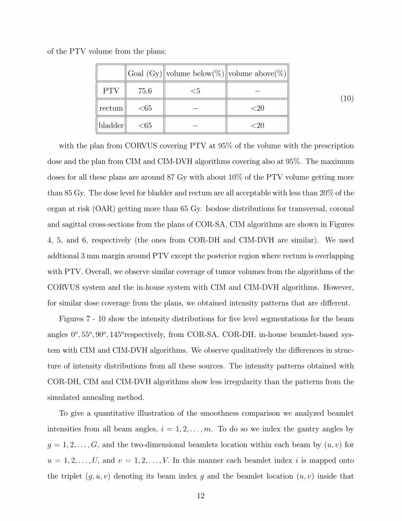
of the PTV volume from the plans;
Goal (Gy) volume below(%) volume above(%)
PTV 75.6 <5 −
rectum <65 − <20
bladder <65 − <20
(10)
with the plan from CORVUS covering PTV at 95% of the volume with the prescription
dose and the plan from CIM and CIM-DVH algorithms covering also at 95%. The maximum
doses for all these plans are around 87 Gy with about 10% of the PTV volume getting more
than 85 Gy. The dose level for bladder and rectum are all acceptable with less than 20% of the
organ at risk (OAR) getting more than 65 Gy. Isodose distributions for transversal, coronal
and sagittal cross-sections from the plans of COR-SA, CIM algorithms are shown in Figures
4, 5, and 6, respectively (the ones from COR-DH and CIM-DVH are similar). We used
addtional 3 mm margin around PTV except the posterior region where rectum is overlapping
with PTV. Overall, we observe similar coverage of tumor volumes from the algorithms of the
CORVUS system and the in-house system with CIM and CIM-DVH algorithms. However,
for similar dose coverage from the plans, we obtained intensity patterns that are different.
Figures 7 - 10 show the intensity distributions for five level segmentations for the beam
angles 0o, 55o, 90o, 145orespectively, from COR-SA, COR-DH, in-house beamlet-based sys-
tem with CIM and CIM-DVH algorithms. We observe qualitatively the differences in struc-
ture of intensity distributions from all these sources. The intensity patterns obtained with
COR-DH, CIM and CIM-DVH algorithms show less irregularity than the patterns from the
simulated annealing method.
To give a quantitative illustration of the smoothness comparison we analyzed beamlet
intensities from all beam angles, i = 1, 2, . . . ,m. To do so we index the gantry angles by
g = 1, 2, . . . , G, and the two-dimensional beamlets location within each beam by (u, v) for
u = 1, 2, . . . , U, and v = 1, 2, . . . , V. In this manner each beamlet index i is mapped onto
the triplet (g, u, v) denoting its beam index g and the beamlet location (u, v) inside that
12

beam. The intensity of the i-th beamlet, which was denoted by xi in Section II, will thus
be denoted by x(g, u, v).
In the prostate case, shown in our example, we have seven gantry angles, i.e., G = 7,
at angles 0o, 55o, 90o, 145o, 215o, 270o and 305o. Within each gantry angle, we have a 2D
intensity map of size 12 × 12, i.e., U = V = 12. The 2D intensity patterns x(g, u, v) for
g = 1, ..., 7 are normalized to its maximum value for that particular beam angle to take
values from 0, 20, ... to 100 ( the five levels). We use the smoothness indicators defined
by Webb, Convery and Evans (Webb et al. 1998, p. 2787). To this end we calculate the
first and second order derivatives of these normalized intensity numbers with respect to the
intensity intervals for each of the beam angle, e.g.,
d
dvx(g, u, v) and
d2
d2vx(g, u, v). (11)
Then we define the mean modulus first derivative of the beamlets as the first smoothness
indicator by
S1 =1
V × UVXv=1
UXu=1
| ddvx(g, u, v) |+ | d
dux(g, u, v) | (12)
and the mean modulus second derivative of the beamlets as the second smoothness indicator
by
S2 =1
V × UVXv=1
UXu=1
| d2
d2vx(g, u, v)|+ | d
2
d2ux(g, u, v)|. (13)
13

S1 S2
Beam Angle COR-SA COR-DH CIM CIM-DVH COR-SA COR-DH CIM CIM-DVH
0o 18.5 12.5 10.1 9.7 16.7 12.5 8.2 8.2
55o 14.5 8.9 10.7 9.0 13.6 7.3 9.6 7.6
90o 14.4 10.7 10.1 8.3 12.9 10.3 9.4 7.4
145o 15.3 14.1 13.1 8.9 14.2 13.6 11.8 7.4
215o 16.3 14.4 11.5 8.8 14.8 13.9 9.1 6.9
270o 14.4 12.8 9.9 8.3 13.4 12.1 9.6 7.4
305o 12.8 7.8 10.1 8.5 11.8 7.3 8.8 7.4
Total 106 81 75 62 97 77 66 52
(14)
In table 14 we list the normalized summation of first and second derivatives of the
normalized intensity numbers (11), namely, the smoothness indicators S1 and S2 for all the
beam angles. Listed in the table are values from COR-SA, COR-CH, the ones from the
in-house system with CIM and CIM-DVH algorithms. Included are values for gantry angles
listed to the left of the table. There are obvious differences between the values of these
smoothness indicators for the intensity patterns obtained from the CORVUS system with
simulated annealing and downhill gradient and those from either the CIM or the CIM-DVH
method. The smoothness values decrease with the following order: COR-SA, COR-DH,
CIM and CIM-DVH, which confirms our qualitative observation from the intensity maps.
The smoothness of the intensity distribution affects the number of segments and monitor
units required for delivery. While the DVHs and the isodose distributions obtained from all
three methods are of similar clinical quality,table (15) shows differences in the number of
segments (for each beam angle) that are required to achieve the intensity distributions shown
in Figures 7 - 10. The numbers of monitor units for delivery of these segments (for each
beam angle) are also listed. The monitor units are for delivery of 75.6 Gy in 42 fractions.
14
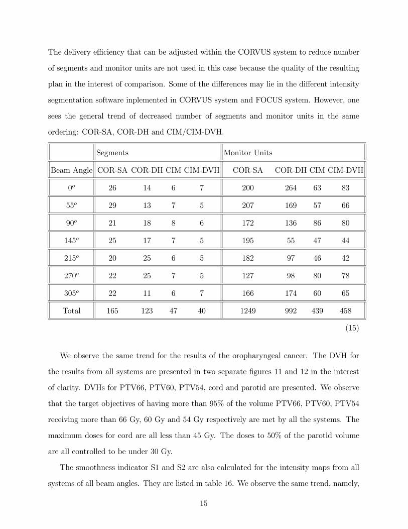
The delivery efficiency that can be adjusted within the CORVUS system to reduce number
of segments and monitor units are not used in this case because the quality of the resulting
plan in the interest of comparison. Some of the differences may lie in the different intensity
segmentation software inplemented in CORVUS system and FOCUS system. However, one
sees the general trend of decreased number of segments and monitor units in the same
ordering: COR-SA, COR-DH and CIM/CIM-DVH.
Segments Monitor Units
Beam Angle COR-SA COR-DH CIM CIM-DVH COR-SA COR-DH CIM CIM-DVH
0o 26 14 6 7 200 264 63 83
55o 29 13 7 5 207 169 57 66
90o 21 18 8 6 172 136 86 80
145o 25 17 7 5 195 55 47 44
215o 20 25 6 5 182 97 46 42
270o 22 25 7 5 127 98 80 78
305o 22 11 6 7 166 174 60 65
Total 165 123 47 40 1249 992 439 458
(15)
We observe the same trend for the results of the oropharyngeal cancer. The DVH for
the results from all systems are presented in two separate figures 11 and 12 in the interest
of clarity. DVHs for PTV66, PTV60, PTV54, cord and parotid are presented. We observe
that the target objectives of having more than 95% of the volume PTV66, PTV60, PTV54
receiving more than 66 Gy, 60 Gy and 54 Gy respectively are met by all the systems. The
maximum doses for cord are all less than 45 Gy. The doses to 50% of the parotid volume
are all controlled to be under 30 Gy.
The smoothness indicator S1 and S2 are also calculated for the intensity maps from all
systems of all beam angles. They are listed in table 16. We observe the same trend, namely,
15

S1 and S2 decrease in the following order: COR-SA, COR-DH, CIM and CIM-DVH.
S1 S2
Beam Angle COR-SA COR-DH CIM CIM-DVH COR-SA COR-DH CIM CIM-DVH
0o 15.2 16.1 14.7 15.3 13.9 15.4 14.3 13.7
40o 15.4 10.2 8.4 8.2 14.5 8.2 7.7 7.3
80o 12.6 11.8 10.1 10.1 12.6 10.2 8.9 9.2
120o 16.8 14.0 12.1 8.6 13.8 14.2 12.3 8.8
160o 19.3 13.2 11.0 10.6 18.9 14.0 11.5 10.5
200o 19.1 13.0 11.1 8.6 17.8 13.3 11.0 8.6
240o 20.6 17.6 15.6 13.8 19.0 16.1 14.6 11.0
280o 15.5 14.2 12.1 9.0 13.6 14.3 12.7 8.9
320o 12.8 16.1 14.3 11.3 11.3 15.6 13.9 11.4
Total 147 126 109 95 136 121 106 89
(16)
The number of segments and monitor units required to deliver these intensity distribu-
tions are listed in table 17. Similarly, some of the difference may be explained by the different
intensity segmentation software incorporated in CORVUS and FOCUS system. However,
the same tendency still holds. The number of segments and monitor units decrease with the
same order: COR-SA, COR-DH, CIM and CIM-DVH.
16

Segments Monitor Units
Beam Angle COR-SA COR-DH CIM CIM-DVH COR-SA COR-DH CIM CIM-DVH
0o 36 24 9 13 198 349 69 66
40o 24 20 7 9 124 245 60 61
80o 26 16 7 10 134 198 46 55
120o 28 12 10 8 194 27 86 72
160o 36 30 9 8 238 68 28 52
200o 28 20 10 8 179 40 52 100
240o 22 20 10 12 86 48 93 99
280o 22 28 16 9 98 62 55 70
320o 32 24 10 12 140 54 129 83
Total 256 197 88 89 1391 1091 618 658
(17)
VI. DISCUSSION
We detected this smoothness phenomenon of Cimmino’s algorithm recently when work-
ing with aperture-based inverse planning (ABIP)(Xiao et al. 2003). It was discovered that
Cimmino’s algorithm always generated in our experimental computational work, when ini-
tialized at zero, solutions that were surprisingly good approximations of the LIF (least-square
intensity feasibility) solution. This was explained and put on firm mathematical ground in
the other publication(Xiao et al. 2003) . In order to achieve the least-square of the total
intensity, extreme intensity values are discriminated against. The smoothness intensity pat-
terns without large variations are thus created. In what follows we explain the inherent
smoothness property of intensity patterns generated by Cimmino’s algorithm. We consider
a vector x = (xi)mi=1 ∈ Rm, translate it, in an agreed manner, into a K × K matrix (so
17

that m = K2) X = (xst)Ks,t=1 whose elements xst are obtained from the components of the
vector x by xst = x(s−1)K+t, for all s, t = 1, 2, . . . ,K, and speak interchangeably about the
vector and the associated matrix. The smoothness of the vector x (or the matrix X) is a
local property that should reflect by how much does a value of one component (bixel) differ
from its surrounding components’ values.
A commonly used smoothness indicator σ(X) of an image represented in a discretized
form by a matrix X = (xst)Ks,t=1 is defined by
σ(X) = (1/8)KX
s,t=1
X(y,z)∈N(s,t)
(xyz − xst)2 (18)
where N(s, t) is the set of indices of the eight surrounding elements neighborhood of the
element (s, t), see, e.g., Li, Jiang and Evans (Li, Jiang and Evans 2000). Since we are
interested in matrices of only nonnegative elements (intensities), this can be equivalently
written as
σ(X) = (1/8)KX
s,t=1
kxst1− exk2 (19)
where 1 is a nine-dimensional vector all of whose components are equal to one and ex isa nine-dimensional vector whose components are equal to the values in the (s, t)∪ N(s, t)square region. Now we show that σ(X) is a convex function.
Proposition 2 Given finitely many vectors xr, for r = 1, 2, . . . , ρ, we have
σ(ρXr=1
αrxr) ≤
ρXr=1
αrσ(xr), (20)
for any set of real positive numbers αr such thatPρr=1 αr = 1.
We have σ(y) = (1/8)PKs,t=1 kyst1− eyk2
= (1/8)PKs,t=1 k
Pρr=1 αr
³xrst1−fxr´ k2
≤ (1/8)PKs,t=1
Pρr=1 αrkxrst1−fxrk2
=Pρr=1 αrσ(x
r), where we have used (19) and the convexity of the function k · k2, and theproof is complete.
18

This shows that the smoothness indicator of any convex combination of vectors is smaller
(not larger, to be precise) then the convex combination of the smoothness indicators of the
individual vectors comprising the convex combination. Since Cimmino’s algorithm takes
convex combinations of the individual projections onto the physical dose constraints at each
and every step it systematically strives to have smoother iterates.
The experiments of inverse treatment planning performed here reveal yet another im-
portant feature of the Cimmino algorithm. Namely, when comparing the intensity patterns
obtained from Cimmino’s algorithm with those obtained from the simulated annealing al-
gorithm, employed by the CORVUS system, which does not have an intrinsic control over
the range of intensities unless used with external filtering(Webb 1989) — the difference in
smoothness of the intensity distribution is significant, as shown in Figures 7 - 10. The
smoothness of the pattern is of significant clinical value because fewer segments are used
for delivery and the total number of monitor units used is reduced. These effects increase
the delivery efficiency and reduce the leakage radiation as compared with what would have
been with a high number of monitor units. Incorporating dose-volume constraints with
Cimmino’s algorithm, neccessitated modifications to the modeling as well as to the iteration
process which involves non-linear terms. However, we observe similar smooth patterns from
the final results as compared with the CIM algorithm. The gradient algorithm is found to
also share some of the smoothness features.
Besides arriving at smooth intensity distributions for beamlet-based inverse planning
problems, the simultaneous property of Cimmino’s algorithm makes it possible to utilize the
available computing resources through parallel computing. Multithreaded implementation
of the Cimmino algorithm which takes full advantage of its parallel characteristic using
a double-processor computer almost halved the performance time in comparison with its
sequential implementation. The simultaneous property is retained in this implementation
of DVH constraints for inclusion of non-linear inequalities(Michalski et al. 2004).
VII. CONCLUSION
19

In implementing and experimentally analyzing Cimmino’s algorithm for beamlet-based
inverse planning problems, we observe an intrinsic property of the algorithm to produce
smooth intensity patterns as applied to beamlet-based IMRT inverse planning which has
not been observed or reported till now. The algorithm not only arrives at solutions that are
close approximations of least-intensity solutions, but also generates intensity distributions
that are mostly smooth. The smooth intensity pattern eases the delivery difficulty and
improves delivery efficiency for both dynamic MLC and MSF—MLC delivery of the IMRT
plans. Fewer segments and monitor units are required. We can reduce the optimization time
many folds utilizing multiple processors due to the simultaneous nature of the algorithm.
Implementation of DVH objectives in the simultaneous projection algorithm didn’t seem to
degrade the level of smoothness from our observation. With the debut of faster and less
expensive computing hardware, real time inverse planning becomes a realty. To summarize,
the combination of inequality constraints for describing the dose upper and lower limits on
organs and the use of Cimmino’s algorithm for the linear feasibility problem arising from
the fully-discretized model of IMRT have the following favorable features and properties:
1. It uses realistic modelling, which does not require equalities to hold for the dose con-
straints.
2. When initialized at zero intensities it generates an approximate LIF solution (which
has least intensity).
3. It converges globally to a feasible solution, if such a solution exists, or to a minimal
value of the proximity function (6) in the inconsistent case.
4. It is an inherently parallel iterative algorithm, thus, implementable on parallel com-
puting equipment regardless of problem structure.
5. It generates smoother intensity distributions.
These properties are shared by the simultaneous projection algorithm that incorporates
DVH dose objectives.
20

VIII. APPENDIX
The Fully Discretized Model and the Feasibility Approach
The beamlet-based inverse planning process assumes full discretization of both the pa-
tient’s cross-section and the radiation intensity field surrounding the patient. Using a state-
of-the-art dose calculation engine we construct a matrix of dose information in which the
matrix element aji is the dose to voxel j due to a unit intensity from beamlet i. We con-
ducted our work with the inverse planning package of the commercial treatment planning
system FOCUS (from Computerized Medical Systems (CMS), Inc., St. Louis, MO, USA).
Having been granted access to this system’s source code, we used the system as our dose
calculation engine. The physician’s imposed dose constraints and their respective weights
of importance were also extracted from the FOCUS system. Then the Cimmino algorithm
(which is not part of the FOCUS system), or the variation of the algorithm incorporating
DVH dose objectives, was applied.
Next, we review how full discretization of the beamlet-based inverse problem in radiation
therapy treatment planning (RTTP) leads to a linear feasibility problem and present the si-
multaneous Cimmino (CIM) method (Censor and Zenios 1997). Assume that the 3D volume
of interest includes Q pre-identified target regions, denoted by {Tq | for q = 1, 2, · · · , Q},for radiation treatment and that the lower bounds for the required dose to be deposited in
target region Tq is tq. The volume of interest also includes S pre-identified critical organs,
denoted by {Bs | for s = 1, 2, · · · , S}, that should be spared by observing upper bounds ofpermissible dose bs in organ Bs. The reminder of the volume constitutes the complimentary
tissue, denoted by C, which is allowed to absorb not more then c dose units. This volume
of interest is discretized into a Cartesian grid of n voxels which are numbered in an agreed
manner by j = 1, 2, · · · , n. Depending on whether a voxel is inside a target (tumor) or insidea critical organ the total dose absorbed in it must lie above or below the lower or upper
prescribed dose bounds, respectively.
The RTTP problem is further discretized by assuming that the radiation, delivered from
21

outside sources, propagates along lines and that the whole volume of interest is uniformly
covered by a mesh of m lines, along which radiation travels (beamlets), densely enough
to reach every voxel in the volume of interest. The beamlets are arranged in a certain
geometry and indexed by i = 1, 2, · · · ,m. The intensities xi of the rays are arranged in anm-dimensional vector x = (xi)
mi=1 ∈ Rm, in them-dimensional Euclidean space Rm, and they
are the unknowns of the problem. These intensities are traditionally called “weights” in this
field but we reserve the latter for the term “weights of importance” of the constraints. We
extract the quantities aji which are the dose absorbed (uniformly) in voxel j due to radiation
of unit intensity along the i-th ray from the FOCUS commercial treatment planning system.
The basic linear feasibility problem (LFP, for short) associated with recovering the beam-
let intensities vector x = (xi)mi=1 is the following.
mXi=1
ajixi ≤ bs, for all j ∈ Bs, s = 1, 2, · · · , S, (21)
tq ≤mXi=1
ajixi, for all j ∈ Tq, q = 1, 2, · · · , Q, (22)
mXi=1
ajixi ≤ c, for all j ∈ C, (23)
xi ≥ 0, for all i = 1, 2, · · · ,m. (24)
The LFP can easily be rearranged into the general form
mXi=1
ajixi ≤ dj, for all j = 1, 2, · · · , n, (25)
which can also be rewritten as
haj, xi ≤ dj, for all j = 1, 2, · · · , n, (26)
where aj = (aji )mi=1 is an m-dimensional vector and haj, xi =
Pmi=1 a
jixi is the inner product
in Rm. The nonnegativity constraints (24) can be either subsumed in the system (26) or
kept separately and handled separately by any iterative algorithm applied to the LFP.
22

In order to incorporate the dose-volume histogram constraints, we use an additional set
of inequalities, the detail of which is described in a recent publication (Michalski et al. 2004).
A brief summary of the modeling is included. For each structure s containing Ns voxels we
have a set of constraints T s. For t ∈ T s, we are allowing αt percent volume getting an over
dose of βt percent of the upper limit bt (similar set of inequalities can be constructed for
lower limits):
haj , xi ≤ (1 + βt)bt, for all j = 1, 2, · · · , Ns, (27)
gt(x) =Xj∈shj(x)− αtNsbtβt ≤ 0 (28)
hj(x) =
0 if haj, xi ≤ bt
haj, xi− btβt + bt if bt ≤ haj, xi ≤ (1 + βt)bt
haj, xi− bt if haj, xi > (1 + βt)bt
(29)
Non-linear terms are introduced in the inequalities to accommodate the dose-volume
constraints.
Acknowledgments. This work was supported in part by Elekta Oncology Systems Inc.,
Norcross, GA, USA. The work of Y. Censor was supported by research grant 592/00 from the
Israel Science Foundation founded by the Israel Academy of Sciences and Humanities. We
gratefully acknowledge the help rendered to this research by Computerized Medical Systems
(CMS), St. Louis, MO, USA, by giving us access to some source code of FOCUS treatment
system software.
23

REFERENCES
Aharoni, R. and Censor, Y.: 1989, Block-iterative projection methods for parallel com-
putation of solutions to convex feasibility problems, Linear Algebra and Its Applications
120, 165—175.
Alber, M. and Nusslin, F.: 2000, Intensity modulated photon beams subject to a minimal
surface smoothing constraint, Physics in Medicine and Biology 45, N49—N52.
Altschuler, M. D. and Censor, Y.: 1984, Feasibility solutions in radiation therapy treatment
planning, Proceedings of the Eighth International Conference on the Use of Computers in
Radiation Therapy, IEEE Computer Society Press, Silver Spring, Maryland, USA, pp. 220—
224.
Auslender, A.: 1976, Optimization: Methodes Numeriques, Masson, Paris, France.
Barakat, R. and Newsam, G.: 1985, Algorithms for reconstruction of partially known, ban-
dlimited Fourier tarnsform pairs from noisy data. II. The nonlinear problem of phase re-
trival, Journal of Integral Equations 9 (Suppl.), 77—125.
Bauschke, H. and Borwein, J.: 1996, On projection algorithms for solving convex feasibility
problems, SIAM Review 38, 367—426.
Bednarz, G., Michalski, D., Houser, C., Huq, M. S., Xiao, Y., Anne, P. R. and Galvin,
J. M.: 2002, The use of mixed-integer programming for inverse treatment planning with
pre-defined field segments, Phys. Med. Biol. 47, 2235—2245.
Bortfeld, T., Burkelbach, J., Boesecke, R. and Schlegel, W.: 1990, Methods of image recon-
struction from projections applied to conformation radiotherapy, Physics in Medicine and
Biology 35, 1423—1434.
Butnariu, D., Censor, Y. and Reich, S. (eds): 2001, Inherently Parallel Algorithms in Feasi-
bility and Optimization and Their Applications, Vol. 8 of Studies in Computational Math-
ematics, Elsevier Science B.V., Amsterdam, The Netherlands.
24

Byrne, C. and Censor, Y.: 2001, Proximity function minimization using multiple Bregman
projections, with applications to split feasibility and Kullback-Leibler distance minimiza-
tion, Annals of Operations Research 105, 77—98.
Censor, Y., Altschuler, M. D. and Powlis, W. D.: 1988a, A computational solution of
the inverse problem in radiation therapy treatment planning, Applied Mathematics and
Computation 25, 57—87.
Censor, Y., Altschuler, M. D. and Powlis, W. D.: 1988b, On the use of Cimmino’s simul-
taneous projections method for computing a solution of the inverse problem in radiation
therapy treatment planning, Inverse Problems 4, 607—623.
Censor, Y. and Zenios, S.: 1997, Parallel Optimization: Theory, Algorithms, and Applica-
tions, Oxford University Press, New York, NY, USA.
Cho, P., Lee, S., Marks, R., Oh, S., Sutlief, S. and Phillips, M.: 1998, Optimization of
intensity modulated beams with volume constraints using two methods: Cost function
minimization and projection onto convex sets, Medical Physics 25, 435—443.
Cho, P., Lee, S., Marks, R., Redstone, J. and Oh, S.: 1997, Comparison of algorithms
for intensity modulated beam optimization: Projection onto convex sets and simulated
annealing, in D. Leavitt and G. Starkschall (eds), Proceedings of the XII International
Conference On the Use of Computers in Radiation Therapy, Medical Physics Publishing,
Madison, WI, USA, pp. 310—312.
Cho, P. and Marks, R. I.: 2000, Hardware-sensitive optimization for intensity modulated
radiotherapy, Physics in Medicine and Biology 45, 429—440.
Cimmino, G.: 1938, Calcolo approssimato per le soluzioni dei sistemi di equazioni lineari,
La Ricerca Scientifica XVI, Series II, Anno IX, 1, 326—333.
Haas, O.: 1999, Radiotherapy Treatment Planning: New System Approaches, Springer-
Verlag, London.
25

Hiriart-Urruty, J.-B. and Lemarechal, C.: 2001, Fundamentals of Convex Analysis, Springer-
Verlag, Berlin, Heidelberg, Germany.
Hoffner, J., Decker, P., Schmidt, E., Herbig, W., Ritter, J. and Wiss, P.: 1996, Develop-
ment of a fast optimization preview in radiation treatment planning, Strahlentherapie und
Onkologie 172, 384—394.
Kolmonen, P., Trevo, J. and Lahtinen, T.: 1998, Use of Cimmino algorithm and continuous
approximation for the dose deposition kernel in the inverse problem of radiation treatment
planning, Physics in Medicine and Biology 43, 2539—2554.
Lee, S., Cho, P., II, R. M. and Oh, S.: 1997, Conformal radiotherapy computation by
the method of alternating projections onto convex sets, Physics in Medicine and Biology
42, 1065—1086.
Li, X., Jiang, T. and Evans, D. J.: 2000, Medical image reconstruction using a multi-
objective genetic local search algorithm, International Journal of Computer Mathematics
74, 301—314.
Michalski, D., Xiao, Y., Censor, Y. and Galvin, J. M.: 2004, The dose-volume constraint
satisfaction problem for inverse treatment planning with field segments, Physics in Medicine
and Biology 49, 601—616.
Powlis, W., Altschuler, M., Censor, Y. and Buhle, E.: 1989, Semi-automated radiotherapy
treatment planning with a mathematical model to satisfy treatment goals, International
Journal Radiation Oncology Biology Physics 16, 271—276.
Spirou, S. and Chui, C.-S.: 1998, A gradient inverse planning algorithm with dose-volume
constraints, Medical Physics 25, 321—333.
Spirou, S., Fournier-Bidoz, N., Yang, J., Chui, C.-S. and Ling, C.: 2001, Smoothing
intensity-modulated beam profiles to improve the efficiency of delivery, Medical Physics
28, 2105—2112.
26
Stark, H. and Yang, Y.: 1998, Vector Space Projections: A Numerical Approach to Signal
and Image Processing, Neural Nets, and Optics, John Wiley, New York, NY, USA.
Starkschall, G.: 1984, A constrained least-squares optimization method for external beam
radiation therapy treatment planning, Medical Physics 11, 659—665.
Webb, S.: 1989, Optimisation of conformal radiotherapy dose distributions by simulated
annealing, Physics in Medicine and Biology 34, 1349—1369.
Webb, S.: 1993, Reprinted with corrections 2001b, The Physics of Three-Dimensional Ra-
diation Therapy, Institute of Physics Publishing (IOP), Bristol, UK.
Webb, S.: 1997, The Physics of Conformal Radiotherapy, Institute of Physics Publishing
(IOP), Bristol, UK.
Webb, S.: 2001a, Intensity-Modulated Radiation Therapy, Institute of Physics Publishing
(IOP), Bristol, UK.
Webb, S., Convery, D. J. and Evans, P. M.: 1998, Inverse planning with constraints to
generate smoothed intensity-modulated beams, Physics in Medicine and Biology 43, 2785—
2794.
Wu, C., Jeraj, R., Lu, W. and Mackie, T. R.: 2004, Fast treatment plan modification with
an over-relaxed cimmino algorithm, Med. Phys. 31(2), 191—200.
Xia, P. and Verhey, L.: 1998, Multileaf collimator leaf-sequencing algorithm for intensity
modulated beams with multiple static segments, Medical Physics 25, 1424—1434.
Xiao, Y., Censor, Y., Michalski, D. and Galvin, J. M.: 2003, The least-intensity feasible
solution for aperture-based inverse planning in radiation therapy, Annals of Operations
Research 119, 183—203.
Xiao, Y., Galvin, J. M., Hossain, M. and Valicenti, R.: 2000, An optimized forward-planning
technique for intensity modulated radiation therapy, Medical Physics 9, 2093—2099.
27

Xing, L. and Chen, T.: 1996, Iterative methods for inverse treatment planning, Physics in
Medicine and Biology 41, 2107—2123.
Xing, L., Hamilton, R., Spelbring, D., Pelizzari, C., Chen, G. and Boyer, A.: 1998, Fast itera-
tive algorithms for three-dimensional inverse treatment planning,Medical Physics 25, 1845—
1849.
28

FIGURES
FIG. 1. The seven beam angles used in the IMRT inverse planning are: 0, 55, 90, 145, 215,
270, 305 degrees (Varian convention).
FIG. 2. The relative locations of the target volumes PTV66, PTV60, PTV54 and critical
structures: cord and parotid.
FIG. 3. DVH comparison between beamlet-based IMRT plans: COR-SA,COR-DH, algorithms
CIM and CIM-DVH.
FIG. 4. Isodose distribution comparison between CORVUS system (upper), in-house algorithms
CIM (lower) for transversal cross-section. The two isodose displays are for 75.6 Gy and 65 Gy
respectively.
FIG. 5. Isodose distribution comparison between CORVUS system (upper), in-house algorithms
CIM (lower) coronal cross-section. The two isodose displays are for 75.6 Gy and 65 Gy respectively.
FIG. 6. Isodose distribution comparison between CORVUS system (upper), in-house algorithms
CIM (lower) for sagital plane. The two isodose displays are for 75.6 Gy and 65 Gy respectively.
FIG. 7. Intensities from left to right for: COR-SA, COR-DH, algorithms CIM and CIM-DVH
shown with outline of PTV for gantry angle 0 degree.
FIG. 8. Intensities from left to right for: COR-SA, COR-DH, algorithms CIM and CIM-DVH
shown with outline of PTV for gantry angle 55 degree.
FIG. 9. Intensities from left to right for: COR-SA, COR-DH, algorithms CIM and CIM-DVH
shown with outline of PTV for gantry angle 90 degree.
FIG. 10. Intensities from left to right for: COR-SA, COR-DH, algorithms CIM and CIM-DVH
shown with outline of PTV for gantry angle 145 degree.
29

FIG. 11. DVH results for the oropharygeal case from COR-SA and CIM for PTV66, PTV60,
PTV54, cord and parotid.
FIG. 12. DVH results for the oropharygeal case from COR-DH and CIM-DVH for PTV66,
PTV60, PTV54, cord and parotid.
30

Figures for the Manuscript:Inherent Smoothness of IntensityPatterns for Intensity ModulatedRadiation Therapy Generated by aSimultaneous Projection Algorithm
Y. Xiao1, D. Michalski1, Y. Censor2 and J. M. Galvin11Medical Physics Division,
Radiation Oncology Department,Thomas Jefferson University Hospital,10th and Locust Streets, Philadelphia,
PA. 19107, USA.({ying.xiao, darek.michalski, james.galvin}@mail.tju.edu).
2Department of Mathematics,University of Haifa, Mt. Carmel,
Haifa 31905, Israel.([email protected]).
May, 2004
1

Figure 1: The seven beam angles used in the IMRT inverse planning are: 0, 55,90, 145, 215, 270, 305 degrees (Varian convention).
2

Figure 2: The relative locations of the target volumes PTV66, PTV60, PTV54and critical structures: cord and parotid.
3

Figure 3: DVH comparison between beamlet-based IMRT plans: COR-SA,COR-DH, algorithms CIM and CIM-DVH.
4

Figure 4: Isodose distribution comparison between CORVUS system (upper),in-house algorithms CIM (lower) for transversal cross-section. The two isodosedisplays are for 75.6 Gy and 65 Gy respectively.
5
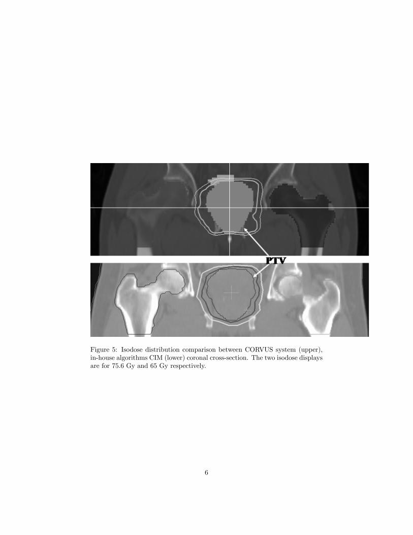
Figure 5: Isodose distribution comparison between CORVUS system (upper),in-house algorithms CIM (lower) coronal cross-section. The two isodose displaysare for 75.6 Gy and 65 Gy respectively.
6

Figure 6: Isodose distribution comparison between CORVUS system (upper),in-house algorithms CIM (lower) for sagital plane. The two isodose displays arefor 75.6 Gy and 65 Gy respectively.
7

Figure 7: Intensities from left to right for: COR-SA, COR-DH, algorithms CIMand CIM-DVH shown with outline of PTV for gantry angle 0 degree.
Figure 8: Intensities from left to right for: COR-SA, COR-DH, algorithms CIMand CIM-DVH shown with outline of PTV for gantry angle 55 degree.
8

Figure 9: Intensities from left to right for: COR-SA, COR-DH, algorithms CIMand CIM-DVH shown with outline of PTV for gantry angle 90 degree.
Figure 10: Intensities from left to right for: COR-SA, COR-DH, algorithms CIMand CIM-DVH shown with outline of PTV for gantry angle 145 degree.
9

Figure 11: DVH results for the oropharygeal case from COR-SA and CIM forPTV66, PTV60, PTV54, cord and parotid.
10
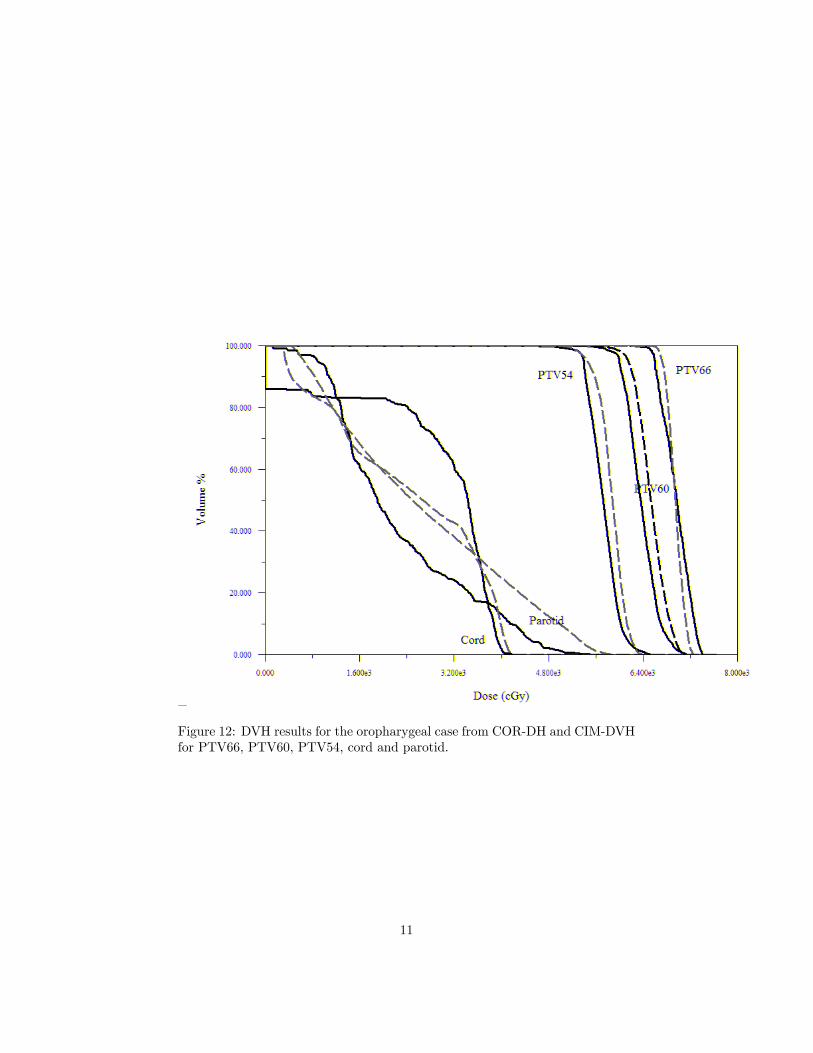
Figure 12: DVH results for the oropharygeal case from COR-DH and CIM-DVHfor PTV66, PTV60, PTV54, cord and parotid.
11