0

INFRARED THERMOGRAPHY IN A HYPERSONIC BOUNDARY LAYER FACILITY

MAE PRACTICAL INTERNSHIP

SUMMER 2012

Mechanical & Aerospace Engineering Department

Princeton University

Name Signature Date

David Harris David Harris August 4, 2012

Laboratory Work and Report Submission Date

Infrared Thermography (Research Work) June 11, 2012

Infrared Thermography (Experimental Work) June 25, 2012

Infrared Thermography (Report Submission) August 20, 2012

Final report submitted September 6, 2012

1

LETTER OF TRANSMITTAL

David Harris

Princeton Undergraduate Class of 2015

Forbes College

Princeton, NJ 08544

August 4, 2012

Alexander J. Smits

Eugene Higgins Professor of

Mechanical & Aerospace Engineering

D218 Engineering Quad

Princeton, NJ, 08544

Dear Professor Smits:

I submit herewith a scientific report for the experiment conducted during my MAE

Practical Summer Internship: Infrared Thermography in a Hypersonic Boundary Layer Wind

Tunnel. It has been turned in according to the due date instructed to by Owen Williams (August

10, 2012) and pledge my honor that I have not violated the Honor Code during the composition

of this lab report.

The report itself contains information and analysis of data retrieved from experiments at

the Hypersonic Boundary Layer Facility (HyperBLaF) at Princeton’s James Forrestal Campus.

It is intended to relay the results of the lab experiments, and provide insight and analysis which

can be used in later experiments.

I hope that your find the report to be informative and comprehensive. I also hope that the

analysis presented within will prove to be fruitful in further developing the foundation required

for hypersonic testing.

Yours sincerely,

David Harris

2

INFRARED THERMOGRAPHY IN A HYPERSONIC BOUNDARY LAYER FACILITY

MAE Practical Internship

Princeton University

Abstract

Hypersonic aircraft travel at high speeds ranging from Mach 6 to Mach 25 (the speed

attained during atmospheric reentry). In these conditions the speed of air particles hitting the

aircraft creates intense friction and generates heat that is very detrimental to the aircraft. These

thermal loads are dominated by convective heat transfer, which is difficult to measure accurately.

An experiment was designed at Princeton’s HyperBLaF (Hypersonic Boundary Layer Facility)

to test a non-intrusive optical measurement technique, known as infrared thermography, with the

aim of obtaining quantitative heat transfer data on a flat brass plate subjected to hypersonic flow.

An infrared camera along with compatible computer software was used to measure surface

temperature over time for a section of Macor in the flat brass plate. This data was then run

through programs written in Matlab to find the heat flux over time and the heat transfer

coefficient for the Macor embedded in the flat brass plate. The equations used in the Matlab

programs use the one-dimensional semi-infinite model to calculate the heat flux and heat transfer

coefficient. Results for heat flux & the heat transfer coefficient were found. However, the

Matlab code and infrared camera readings require further validation before final conclusions can

be made.

HyperBLaF Facility

The HyperBLaF is a Mach 8 blowdown tunnel (Figure

1) used for studies of compressible turbulence, shock

wave/boundary layer interactions, shock/shock interactions

and configuration studies for hypersonic vehicles. The test

section has a diameter of 229 mm (9”), with a length of 2.0m

(6 ft). The max stagnation temperature is 870K (1100 F) at a

max stagnation pressure of 10 MPa (1500 psia). Run times

vary from approximately 2 to 10 minutes. The range of

possible Reynolds numbers allow for completely laminar flow

at the lowest value and completely turbulent boundary layers

on a flat plate at its highest value. When the tunnel turns on,

air from an outdoor storage facility is heated by traveling

through an electrically preheated pipe. Flow properties are

considered constant through the test section. Figure 1: HyperBLaF Wind Tunnel

3

Infrared Camera

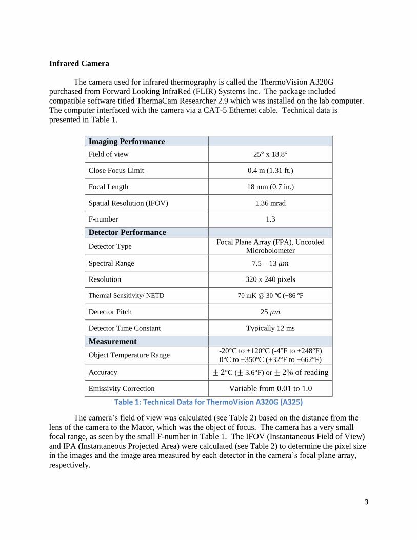
The camera used for infrared thermography is called the ThermoVision A320G

purchased from Forward Looking InfraRed (FLIR) Systems Inc. The package included

compatible software titled ThermaCam Researcher 2.9 which was installed on the lab computer.

The computer interfaced with the camera via a CAT-5 Ethernet cable. Technical data is

presented in Table 1.

The camera’s field of view was calculated (see Table 2) based on the distance from the

lens of the camera to the Macor, which was the object of focus. The camera has a very small

focal range, as seen by the small F-number in Table 1. The IFOV (Instantaneous Field of View)

and IPA (Instantaneous Projected Area) were calculated (see Table 2) to determine the pixel size

in the images and the image area measured by each detector in the camera’s focal plane array,

respectively.

Imaging Performance

Field of view 25 x 18.8

Close Focus Limit 0.4 m (1.31 ft.)

Focal Length 18 mm (0.7 in.)

Spatial Resolution (IFOV) 1.36 mrad

F-number 1.3

Detector Performance

Detector Type Focal Plane Array (FPA), Uncooled

Microbolometer

Spectral Range 7.5 – 13

Resolution 320 x 240 pixels

Thermal Sensitivity/ NETD 70 mK @ 30 (+86

Detector Pitch 25

Detector Time Constant Typically 12 ms

Measurement

Object Temperature Range -20 C to +120 C (-4 F to +248 F)

0 C to +350 C (+32 F to +662 F)

Accuracy C ( 3.6 F) or 2% of reading

Emissivity Correction Variable from 0.01 to 1.0

Table 1: Technical Data for ThermoVision A320G (A325)

4

Equipment Validation

Based on the radiation theory presented in the Appendix 1, the camera requires inputs

describing the surrounding environment, interfering mediums, and the object being studied in

order to return accurate temperature data. First, the Macor insert, the object being studied, is

considered to be a grey-body, so the emissivity had to be measured and compared to another

source for validation. Likewise the wind tunnel viewing window (4” wide and 0.5” thick), made

out of zinc selenide, has a transmissivity factor that had to be measured and compared to data

from the manufacturer.

Figure 2A: Schematic of the different mediums accounted for to conduct infrared thermography

Spatial Resolution

Distance from Camera 0.4 m (1.31 ft) = Close Focal Limit

Width Height Area

FOV 6.982 in. 5.214 in. 36.404

IFOV 0.210 in. 0.210 in. 0.044

IPA 0.406 in. 0.406 in. 0.165

Table 2: Optical Field of View at Minimum Focal Distance

5

This validation was accomplished by conducting three test trials in a simulated wind

tunnel setup (Figure 2). The ThermaCam Researcher software contains an algorithm for

estimating the emissivity and transmissivity based on the input of a “known” and an “un-

calibrated” temperature measurement. The “known” temperature is recorded for a piece of

electrical tape attached to the Macor. This tape has a known emissivity so the temperature

recorded is considered to be the real temperature. The “un-calibrated” temperature is recorded

for the Macor next to the tape, whose emissivity is not known. The environmental conditions for

the three trials are recorded in Table 3, with the “known” and “un-calibrated” temperature inputs

specified.

Environment

Conditions Trial 1 Trial 2 Trial 3

Reflected

Apparent

Temperature ( )

26.7 31.0 26.5

Ambient

Temperature ( ) 26.0 26.5 26.1

Relative

Humidity 41% 41% 41%

Temperature

Measurements

( )

Known Un-calibrated Known Un-calibrated Known Un-calibrated

59.7 59.3 55.0 54.0 52.3 52.1

Table 3: Radiation Parameter Measurements

The emissivity values obtained during these three trials (see Table 4) were averaged to

obtain the value for emissivity used to calibrate the camera for the actual wind tunnel test. The

emissivity values for the Macor were compared to a graph (Figure 3) found in the paper Infrared

Thermography for Convective Heat Transfer Measurements by Carlomagno and Cardone

Figure 2B: Simulated Wind Tunnel Setup

Infrared Camera

Wind Tunnel

Window

Macor

6

because no data regarding emissivity was provided by Macor manufacturers. The emissivity

values from the FLIR for the Macor compare favorably with the values shown in Figure 3.

The wind tunnel window transmissivity measurements (see Table 4) were compared to a

graph of transmissivity (Figure 4) with respect to wavelength provided by the company for zinc

selenide windows of similar thickness (~ half). The averaged transmissivity values were

sufficiently close to the manufacturer/researcher values.

Trial 1 Trial 2 Trial 3 Average

Emissivity 0.938 0.903 0.895 0.912

Transmissivity 0.676 0.70 0.680 0.685

Table 4: Measurements for Infrared Camera Algorithm

Experimental Setup: Wind Tunnel Model

The wind tunnel test model consisted of Macor, a white glass ceramic, embedded in a

sharp, flat, brass plate (Figure 7). Macor was chosen because it has properties suitable for

studying transient heat conduction, such as low thermal conductivity and low thermal diffusivity.

It also has a relatively high emissivity which facilitates the task of calibrating the infrared

camera.

Figure 4: Manufacturer Transmission Graph for Zinc Selenide Window

Figure 3: Directional Emissivity of MACOR (Carlomagno & Cardone, 2010)

Side View

7

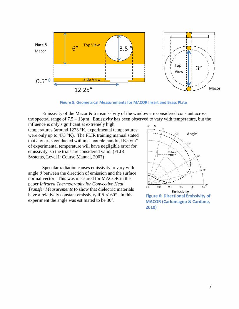
Emissivity of the Macor & transmissivity of the window are considered constant across

the spectral range of 7.5 – 13 . Emissivity has been observed to vary with temperature, but the

influence is only significant at extremely high

temperatures (around 1273 K, experimental temperatures

were only up to 473 K). The FLIR training manual stated

that any tests conducted within a “couple hundred Kelvin”

of experimental temperature will have negligible error for

emissivity, so the trials are considered valid. (FLIR

Systems, Level I: Course Manual, 2007)

Specular radiation causes emissivity to vary with

angle between the direction of emission and the surface

normal vector. This was measured for MACOR in the

paper Infrared Thermography for Convective Heat

Transfer Measurements to show that dielectric materials

have a relatively constant emissivity if 60 . In this

experiment the angle was estimated to be 30 .

Figure 5: Geometrical Measurements for MACOR Insert and Brass Plate

Figure 6: Directional Emissivity of MACOR (Carlomagno & Cardone, 2010)

Emissivity

Angle

Top View

Side View

Top

View

Plate &

Macor

Macor

8

Experimental Setup: Tunnel Setup & Software Calibration

The camera was set up on a tripod facing the wind tunnel window at an angle of ~ 30 as

shown in Figure 7. The data entered into the ThermaCam Researcher software for calibration is

listed in Table 5. The Spot Tool referenced in Table 5 is a small pointer used in ThermaCam

Researcher to specify the spot at which the user would like to measure temperature over time.

The pixel coordinates indicating where the Spot Tool was placed on the images of the Macor is

provided. A distance and emissivity value is supplied for the Spot Tool because measurement

tools in ThermaCam Researcher can be calibrated for different emissivities and object ranges.

Image Frequency 30 Images/Second

Spot Tool

X-Position (from Bottom Left) 111 pixels

Y-Position (from Bottom Left) 157 pixels

Object Distance 0.4 meters

Emissivity 0.91

Object Parameters

Emissivity 0.91

Object Distance 0.4

Reflected Temperature 26

Atmospheric Temperature 26.7

Atmospheric Transmission 1

Relative Humidity 0

Reference Temperature -273.1

External Optics Temperature 40

External Optics Transmission 0.68

Table 5: Input Values for the Infrared Camera Software used in Wind Tunnel Test

Figure 8: Side View of Experiment Setup

Figure 7: Top View of Experiment Setup

9

Experimental Execution: Data Collection

The infrared camera recorded infrared images at 30 Hz and sent the images through the

CAT-5 Ethernet Cable to the computer where they were saved in FLIR’s ThermaCam

Researcher software. Each infrared image consists of an array of 76,800 pixels; equal to the

number of detectors installed on the camera’s focal plane array. Each detector generates a signal

based on the amount of infrared radiation absorbed in its IFOV. A color palette applied to the

image distinguishes areas of similar temperature. Surface temperature measurements on one

spot of the Macor are equal to the size of one pixel (which equals the area of the IFOV) was

recorded for each infrared image and saved in a text file (Table 6). All measurements were made

at the same spot across the entire run time of the tunnel. These surface temperature

measurements are graphed with respect to time in Figure 9.

ThermaCam Researcher output the temperature data measured over time at one spot as a text

file with several columns. The data used in the Matlab programs are the surface temperature data in

column 1 and the time values in column 2 (shaded in Table 6).

Temperature

( Kelvin)

Relative Time

(seconds) Date & Time

# Images

Taken

Initial

Temperature

&

Initial Time

297.213 1344376159.625 8/7/2012

5:49:19.625 PM 1

297.052 1344376159.658

8/7/2012

5:49:19.658 PM 2

297.052 1344376159.692 8/7/2012

5:49:19.692 PM 3

297.025 1344376159.725 8/7/2012

5:49:19.725 PM 4

Table 6: Text File output by ThermaCam Researcher with Surface Temperature Data

Figure 9: Surface Temperature Graph over time recorded by FLIR Infrared Camera

10

The Semi-Infinite Model

Only the heat transfer methods of conduction and convection (see Table 8) are measured

in this experiment. Radiation heat transfer, which is proportional to (see Table 4), is assumed

to be negligible due to the relatively low temperatures in this experiment (298.13 –

373.13 ). As seen in the following energy balance equation, conductive and convective heat

fluxes are considered equal (Figure 10) and radiation heat flux is considered negligible:

The semi-infinite model assumes that heat transfer is one-dimensional and is occurring

through a product of low thermal diffusivity (a property satisfied by Macor material). It is called

the “thick-wall” technique because it uses the assumption that the material is infinitely thick.

The initial conditions are that at time the temperature is the initial wall temperature (see

Table 7). The model breaks down once heat has penetrated through half the thickness of the

material (1.5 cm (0.59 in.).

Heat Transfer Method

“Thick Wall”

Equation Explanations

Conduction

Convection )

Radiation

Table 8: General Heat Transfer Equations

Initial Wall Temperature 297.213

Final Wall Temperature 437.079

Total Change in Temperature 139.866

Table 7: Temperature Boundaries for the Measurement Spot on Macor

Figure 10: Semi-Infinite Model Illustration is convective heat transfer, is radiative heat

transfer, and is conductive heat transfer].

Penetration Depth

= 1.5 cm

𝑅

11

Transient Heat Conduction Criteria

The period between the beginning of a heat transfer process and when the device reaches

steady state is known as the transient period where temperature varies with time and position.

Measuring heat flux allows us to understand the thermal loads on the object during the transient

period. The criterion that determines how long a body undergoes transient heat conduction

before reaching steady state is defined by Equation (1) in Table 9. A Matlab program was

written to display a graph indicating when the solution violates the boundary condition. (See

Figure 11).

The measuring time for which the semi-infinite model assumption holds is dictated by

Equation (2) (Astarita, Cardone, & Carlomagno, 2006) in Table 9.

Criteria Equation Variables Time Limit for

this Test

Tunnel Run-Time for

this test Known “ ~179.00 seconds

Transient Heat

Conduction Criteria (1)

= Penetration Depth

= thermal diffusivity

= Measurement Time

~55.00 seconds

Time Measurement

Criteria for thick-wall

technique (2)

= Penetration Depth

= Thermal Diffusivity

= Measurement Time

27.49 seconds

Table 9: Time Approximations based on material properties and dimensions

Figure 11: Graph of Transient Heat Conduction Criteria over Time

12

Heat Flux Calculations

The equation derived to calculate heat flux based on temperature change across time for a

semi-infinite body is: (Astarita, Cardone, & Carlomagno, 2006)

Where = is the surface temperature difference, is the mass density, is the

specific heat, and is the thermal conductivity. It is assumed that the entire object is the same

temperature at time = 0. However, the integral becomes infinity at the upper boundary

condition which makes the equation unsuitable for use in a computer program. A different form

of the equation that approximates the solution using a piecewise function was developed in

(Cook & Felderman, 1965); where , , and are specific times within the summation and is the total time elapsed in a particular summation interval.

–

(1)

This approximation is further simplified by expanding the sum of the first two terms to

get the equation into this final form:

(2)

Equations (1) and (2) were run in Matlab using the surface temperature measurements

from the infrared camera as input and outputting a graph of heat flux over time. The order of

magnitude for heat flux is about 2-4 kilowatts in an area the size of the IFOV described earlier in

this paper (the unit label for the y-axis is inaccurate with regard to the ). The equations

should have output graphs that were visually similar, but as seen in Figure 9 there is some

discrepancy between the outputs of the two equations. One explanation is that the violation of

the transient heat conduction criteria at t = 50s caused the equations to diverge. Another possible

cause is a bug in the code relating to summations. A previous bug was discovered that caused

the solutions to cluster about the zero position because there was an error in the summation code.

Lastly, it is possible that the initial conditions for Equation (2) differ from Equation (1) and

weren’t accounted for in the code. Since the slopes of the graph change dramatically at 50

seconds, the first explanation appears to be the more likely cause. An attempt will be made in

future experiments to apply a smoothing technique to minimize the random noise.

13

Findings: Heat Flux

With regard to heat flux, the implementation of the Cook-Felderman approximation in a

Matlab program proved successful in generating heat flux readings of the expected order of

magnitude. Random noise is present so more precise readings can hopefully be obtained in

future experiments using data smoothing techniques such as the “least squares” approximation.

The discrepancy between Equation (1) and (2) will also be addressed in for future experiments.

Heat Transfer Coefficient Calculations

The Heat Transfer Coefficient estimate is 28

An effective formula for determining heat transfer coefficients is found in (Astarita, Cardone, &

Carlomagno, 2006). This form is used when the heat transfer rate and the reference temperature

are constant. is the constant reference temperature, is the initial wall temperature, and

is the current wall temperature. In addition, is the complementary error function, and

, , and are mass density, specific heat, and thermal conductivity, respectively.

(3)

(4)

Using a Matlab program, Equation (4) is solved for and substituted into Equation (3) for

values of the heat transfer coefficient ranging from 0 to 500. Values of 870 and 297.213

are used for and respectively. The difference between the value generated for based

on is compared to the value of in the text file generated by ThermaCam Researcher

software. A plot of these differences or “errors” for each heat transfer coefficient value is shown

Figure 12: Output for Equation (1): Red Line = Equation (1), Blue line = Equation (2)

14

in Figure 13. The value with the lowest error is considered to be the best estimate for the heat

transfer coefficient.

Findings: Heat Transfer Coefficient

Based on the graph it appears that the best estimate for the heat transfer coefficient is a

value of 28. Unfortunately, the tolerance for this program is based on how many value are

chosen to be sampled between 0 and 500. Another program could be written to search with a

higher tolerance between the values of 27 and 29 to find a more precise value for the heat

transfer coefficient, but this is slightly inefficient. This also does not return show how the heat

transfer coefficient changes with time.

To summarize, an estimate of the heat transfer coefficient was determined using a Matlab

program. The technique described above for calculating the heat transfer coefficient has the

potential to deliver a more precise estimate but requires revision of the code based on the range

of values to sample. More importantly, the program needs to show how the heat transfer

coefficient changes with time. This can be accomplished by simply implementing the equation

for convective heat flux: )

This requires that the previous heat flux program that calculates be verified and the free-

stream temperature in the wind tunnel be matched in time with the temperature measurements , in

the ThermaCam Researcher text file.

Considerations for Future Experiments in Heat Transfer

Stanton Number

A future goal for this experiment is to calculate the non-dimensional Stanton Number

using tunnel properties and the heat flux values found in Table 10.

Figure 13: Output for Equation (3): The point of minimum is equal to the estimated heat transfer coefficient = 28.

Minimum Error

15

Heat Transfer Gage Research

Initial research was conducted to determine what type of heat sensor is best to validate

the presumed absolute temperature readings from the infrared camera. Criteria for the sensors

are quite restrictive. First, the sensor must operate on the thin-film semi-infinite medium

assumption. Second, the sensor must be small so as to minimize interference with the flow

around the model, but also large enough to be observed properly with the infrared camera

(diameter no less than

of an inch). Lastly, the sensor must be able to withstand the tunnel

conditions, which cover run times from 2 to ten minutes long, and a stagnation temperature as

high as 500 .

Two options are currently available that meet these criteria. The first is a differential

thermopile sensor (called HFM’s) from a company called Vatell. These sensors have the lowest

time constant in the field (300 ). They also present the option of purchasing either a resistance

temperature sensor or a thermocouple design. They can withstand up to 700 . The sensors are

short enough to be fully embedded in the Macor. These sensors ship along with software

designed to compute heat flux over time. Thermopiles are known to have good-signal-to noise

ratio and the Resistance Temperature Sensor outputs an accurately linear “temperature vs.

resistance” graph. However, the advantages of these heat flux sensors are offset by the fact that

they cost three times as much as other competing sensors.

The competing sensor is a heat flux transducer that uses a Gardon Gage design. The

device can withstand up to 500 in the wind tunnel via heat sink/water cooling. The sensitivity

is on the order of milli-volts instead of micro-volts for the HFM’s. The time constant is on the

order of milliseconds as opposed to microseconds for the HFM’s. This sensor has a more

affordable cost comes with an optical black coating that gives it a high emissivity (favorable for

infrared thermography). An optical coating is optional for the HFM sensors.

Stanton Number

(Dimensionless Parameter)

𝑅

Table 10: Description of the Stanton Number for Future Calculations

16

Literature Cited (References) 1Carlomagno, Giovanni M.; Cardone, Gennaro. (last edited August 3, 2010). Infrared

Thermography for convective heat transfer measurements. Exp Fluids (2010) 49:1187-

1218.

2

( November 19, 2007). User’s manual: ThermoVision A320;TermoVision A320G. FLIR

Systems,Inc.

3 (2007) ThermoVision A320G: Infrared Camera System. FLIR Systems, Inc

4 Simeonides, George. (1992). Infrared Thermography in Blowdown and Intermittent Facilities.

VKI

5

(2007). FLIR Systems, Inc. Level I Course Manual. Infrared Training Center: N. Billerica:

Massachusets

9Corning Incorporated. Lighting & Materials. Corning: New York

6T. Astarita, Cardone, Gennaro,Carlomagno, Giovanni M. (last edited May 23, 2005). Infrared

Thermography: An optical method in heat transfer and fluid flow visualization. Optics &

Lasers in Engineering 44 (2006) 261-281

7de Luca, Luigi; Cardone, Gennaro. Viscous Interaction Phenomena in Hypersonic Wedge

Flow. AIAA VOl. 33, No. 12, pp. 2293-2298

8Rathore, M.M.; Kapuno, Jr., Raul R.A. Engineering Heat Transfer: Second Edition. Jones &

Bartlett Learning: Ontario. (2011)

9Cook, W.J.; Felderman, E.J. Reduction of Data from Thin-Film Heat-Transfer Gages: A

Concise Numerical Technique. AIAA Vol. 4, No. 3, pp 561-562.

10

Cook, W.J. Determination of Heat-Transfer Rates from Transient Surface Temperature

Measurements. AIAA Vol. 8, No. 7, pp. 1366-1368

17

Appendix 1

Infrared Thermography (IRTh) requires an understanding of radiation starting with the concept

of the electromagnetic spectrum and the existence of blackbodies. Good overviews are found in

(Buchlin, 2010), (Meola & Carlomagno, 2004), and (Carlomagno & Cardone, 2010), as well as

in the software documentation for all FLIR infrared thermography products. Planck’s law

dictates the emissive power (i.e. radiative heat flux) of a blackbody as a function of wavelength:

is absolute temperature, is the wavelength, is Boltzmann’s constant, and is Planck’s

constant. Boltzmann’s law follows from the integration of Planck’s law across all wavelengths,

giving the total emissive power of a blackbody over the entire spectrum.

The Stefan-Boltzmann constant (a simple constant of proportionality) is equal to

. Most real objects, however, are not blackbodies and only emit a fraction of their

actual blackbody emissive power for any specific temperature. These are called grey-bodies and

a correction factor known as emissivity is added to Boltzmann’s law to calculate heat flux for

grey-bodies. Emissivity can be a constant, but usually is a function varying with surface state,

temperature, and viewing angle (Simeonides, 1992). The equation of radiative heat flux for a

grey-body is:

The following equation dictates all the radiation from an object that the camera can see.

Absorbance , reflectance , and transmittance are all ratios of greybody radiance to blackbody

radiance over blackbody radiance at a specific wavelength:

It is usually assumed that the grey-body follows Kirchhoff’s Law, which is described by the

equality below.

For opaque bodies, transmittance is equal to zero, and the equation becomes:

Lastly, the Wien Displacement Law is obtained by differentiating Planck’s law. The expression

relates a particular wavelength to its max blackbody temperature,

Units of (

is the temperature in degrees Kelvin and is wavelength in micro-meters. Based on this

theory, the emissivity, transmissivity, and reflectivity had to be calculated using a well-

documented procedure.

0

Appendix 2 Company Vatell Vatell Medtherm SWL Germany SWL Germany SWL Germany SWL GermanySensor Name HFM - 8 - E/H HFM - 7 - E/H Heat Flux Transducer

Model Number None None 4-200-.125-36-20942 Standard model KL MI MI with thread M 3.5 MI with pressure tap and adapter

Important Properties

Heat Flux Range Not Advertised Not Advertised 200 Btu/ft^2.sec

Peak Operating Temperature 700 C 700 C 400 C

Uncoated Response Time 17 µs 17 µs ~10ms

Coated Responset Time 300 µs 300 µs Not Applicable

Sensor-Specific Properties

Pressure Tap No No No No No No Yes

Temperature Sensor Thermocouple--Type E RTS Not Applicable Thermocouple--Type E or Type K Thermocouple--Type E or Type K Thermocouple--Type E or Type K Thermocouple--Type E or Type K

Heat Flux Sensor Differential Thermopile Differential Thermopile Transducer--Gardon Gage

RTS Metal Not Applicable Platinum Not Applicable

RTS Resistance Not Applicable 100-200 ohms Not Applicable

Temperature Sensor Resistance Not Applicable 0.25-0.35 ohms/ C Requires Heat Sink/Cooled Model

Min. Sensitivity 150 µV/W/cm^2 150 µV/W/cm^2 10 mV at 200 Btu/ft^2.sec

Physical Attributes

Diameter 0.25 in. 0.25 in. 0.0625 in. 1.9 mm 4.8 mm/3.6 mm 3.5 4.8 mm/3.6 mm

Lead Wire Material (Temp Resist.) Mineral Sheath (350 C) Mineral Sheath (350 C) AWG Solid Copper w/ Teflon Inslation

Lead Wire Length ~ 36 in. ~ 36 in. 36 in.

Body Length 0.96 in. 0.96 in. 0.125 in. 20 mm 12 mm 12 mm 12 mm

Sensor Material Nichrome/Constantan Nichrome/Constantan

Body Material Nickel Housing Nickel Housing OFHC Copper/ Aluminum Alloy chromel/constantan--chromel/alumel chromel/constantan--chromel/alumel chromel/constantan--chromel/alumel chromel/constantan--chromel/alumel

Lab/Experimental Concerns

Price $3,285 $3,285 $1,331.00

Shipping Time 3-4 weeks 3-4 weeks ~ 5 weeks

Mounting (Thread or Flush Mount) 1/2-20 THD or M12 x 1.75 1/2-20 THD or M12 x 1.75 Not Specified

Coating Otpional Coating--Emissivity = 0.94 Optional Coating--Emissivity = 0.94 Standard "Optical Black" Coating

Output Heat Flux & Temperature Heat Flux & Temperature Heat Flux

Data Acquisition

Connection 4-pin Lemo Connector 4-pin Lemo Connector Need to call company back

Thermocouple Characterization Function T = a * V^3 + b * V^2 + c * V + d T = a * V^3 + b * V^2 + c * V + d

Base Temperature Resistance Not Applicable R_o = e * T_o + f

Resistance relation to Voltage Output Not Applicable ((V_rts) / (I_rts * G_rts)) + R_o

Thermocouple Voltage Output V_tc/G_tc Not Applicable

Heat Flux Computation q = (V_hfs/G_hfs) / (g * T + h) Not Applicable

Convection Computation q = h * del_T = (V_o(E))/ S_in q = h * del_T = (V_o(E))/ S_in

Compare/Contrast

Linearity of Output Non-linear output for thermocouple Linear Output for RTS

Extra Purchase Items Vatell AMP-6 (Amplifier) Vatell AMP-6 (Amplifier)

Sensor Performance thermopile = good signal-noise ratio thermopile = good signal-noise ratio

0