Informed search algorithms

Chapter 4

Material

•

Chapter 4 Section 1 -

3•

Exclude memory-bounded heuristic

search

Outline•

Best-first search

•

Greedy best-first search•

A*

search

•

Heuristics•

Local search algorithms

•

Hill-climbing search•

Simulated annealing search

•

Local beam search•

Genetic algorithms

Review: Tree search

•

\input{\file{algorithms}{tree-search-short- algorithm}}

•

A search strategy is defined by picking the order of node expansion

Best-first search•

Idea: use an evaluation function

f(n) for each node

–

estimate of "desirability" Expand most desirable unexpanded node

•

Implementation:Order the nodes in fringe in decreasing order of

desirability

•

Special cases:–

greedy best-first search–

A*

search

Romania with step costs in km

Greedy best-first search

•

Evaluation function f(n) = h(n) (heuristic)•

= estimate of cost from n

to goal

•

e.g., hSLD

(n)

= straight-line distance from n to Bucharest

•

Greedy best-first search expands the node that appears

to be closest to goal

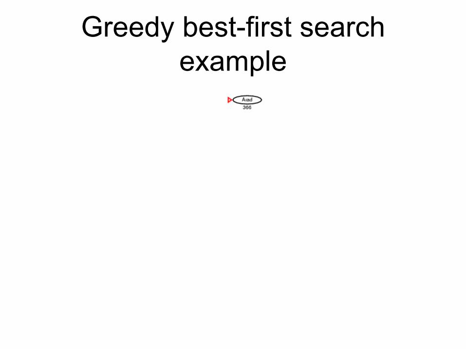
Greedy best-first search example

Greedy best-first search example

Greedy best-first search example

Greedy best-first search example

Properties of greedy best-first search

•

Complete?

No –

can get stuck in loops, e.g., Iasi Neamt Iasi Neamt

•

Time?

O(bm), but a good heuristic can give dramatic improvement

•

Space?

O(bm) --

keeps all nodes in memory

•

Optimal? No

A*

search

•

Idea: avoid expanding paths that are already expensive

•

Evaluation function f(n) = g(n) + h(n) •

g(n) = cost so far to reach n

•

h(n)

= estimated cost from n

to goal•

f(n) = estimated total cost of path through n

to goal

A*

search example

A*

search example

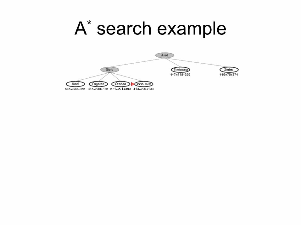
A*

search example

A*

search example

A*

search example

A*

search example

Admissible heuristics

•

A heuristic h(n)

is admissible

if for every node n,h(n) ≤

h*(n), where h*(n)

is the true cost to reach

the goal state from n

.•

An admissible heuristic never overestimates

the

cost to reach the goal, i.e., it is optimistic •

Example: hSLD

(n) (never overestimates the actual road distance)

•

Theorem: If h(n) is admissible, A*

using TREE-

SEARCH is optimal

Optimality of A*

(proof)•

Suppose some suboptimal goal G2

has been generated and is in the fringe. Let n

be an unexpanded node in the fringe such that n is on a shortest path to an optimal goal G

.

•

f(G2

) = g(G2

) since h(G2

) = 0 •

g(G2

) > g(G) since G2

is suboptimal •

f(G) = g(G)

since h(G) = 0 •

f(G2

) > f(G)

from above

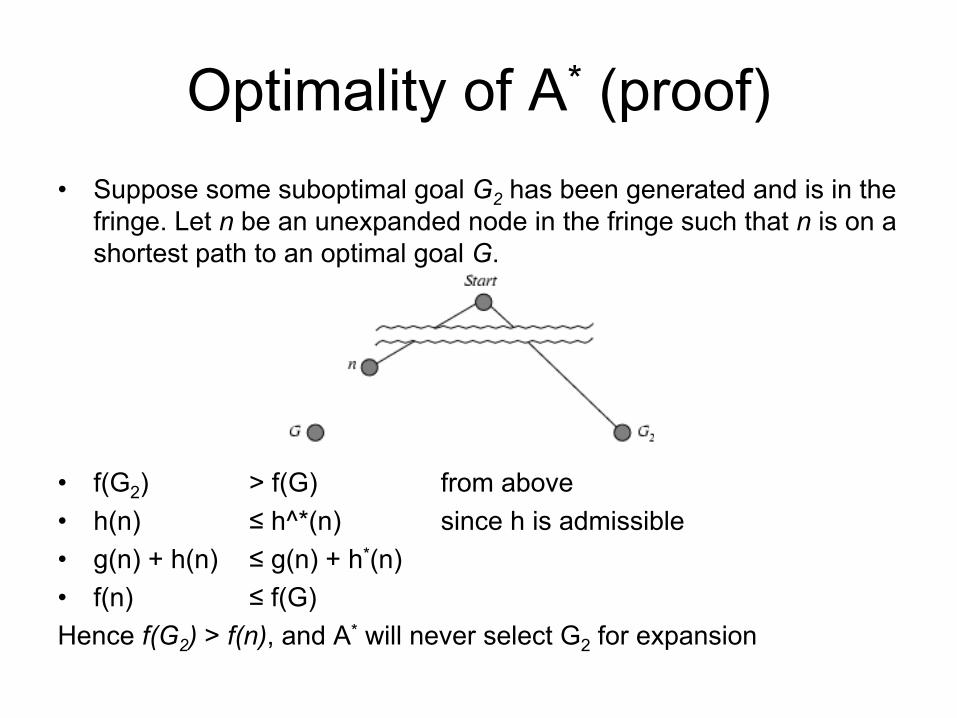
Optimality of A*

(proof)•

Suppose some suboptimal goal G2

has been generated and is in the fringe. Let n

be an unexpanded node in the fringe such that n is on a shortest path to an optimal goal G

.

•

f(G2

)

> f(G) from above •

h(n)

≤

h^*(n)

since h is admissible•

g(n) + h(n)

≤

g(n) + h*(n) •

f(n) ≤

f(G

)Hence f(G2

) > f(n), and A*

will never select G2

for expansion

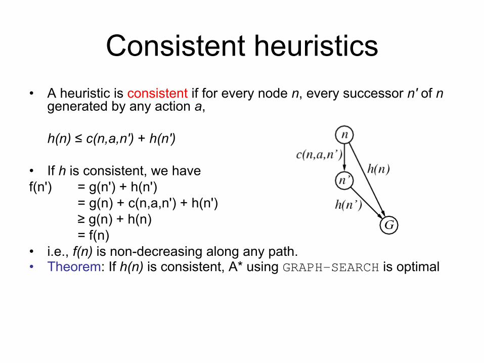
Consistent heuristics•

A heuristic is consistent

if for every node n, every successor n'

of n

generated by any action a

,

h(n) ≤

c(n,a,n') + h(n')

•

If h

is consistent, we havef(n') = g(n') + h(n')

= g(n) + c(n,a,n') + h(n') ≥

g(n) + h(n) = f(n

)•

i.e., f(n)

is non-

decreasing along any path.•

Theorem: If h(n)

is consistent, A*

using GRAPH-SEARCH is optimal

Optimality of A*

•

A*

expands nodes in order of increasing f

value

•

Gradually adds "f-contours" of nodes •

Contour i

has all nodes with f=fi

, where fi

< fi+1

Properties of A$^*$

•

Complete?

Yes (unless there are infinitely many nodes with f ≤

f(G) )

•

Time?

Exponential•

Space?

Keeps all nodes in memory

•

Optimal?

Yes

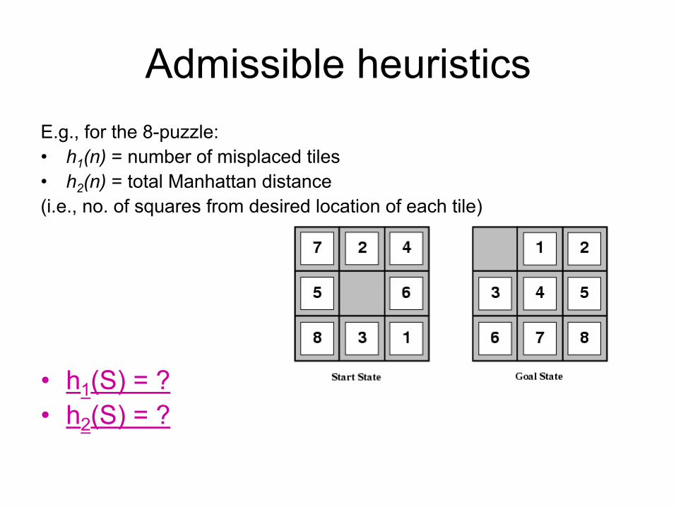
Admissible heuristicsE.g., for the 8-

puzzle:•

h1

(n) = number of misplaced tiles•

h2

(n) = total Manhattan distance (i.e., no. of squares from desired location of each tile)

•

h1

(S) = ? •

h2

(S) = ?

Admissible heuristicsE.g., for the 8-

puzzle:•

h1

(n) = number of misplaced tiles•

h2

(n) = total Manhattan distance (i.e., no. of squares from desired location of each tile)

•

h1

(S) = ?

8•

h2

(S) = ?

3+1+2+2+2+3+3+2 = 18

Dominance•

If h2

(n) ≥

h1

(n)

for all n

(both admissible)•

then h2

dominates

h1•

h2

is better for search

•

Typical search costs (average number of nodes expanded):

•

d=12

IDS = 3,644,035 nodes A*(h1

) = 227 nodes A*(h2

) = 73 nodes •

d=24 IDS = too many nodes

A*(h1

) = 39,135 nodes A*(h2

) = 1,641 nodes

Relaxed problems•

A problem with fewer restrictions on the actions is called a relaxed problem

•

The cost of an optimal solution to a relaxed problem is an admissible heuristic for the

original problem•

If the rules of the 8-puzzle are relaxed so that a tile can move anywhere, then h1

(n) gives the shortest solution

•

If the rules are relaxed so that a tile can move to any adjacent square,

then h2

(n) gives the shortest solution

Local search algorithms•

In many optimization problems, the path

to the

goal is irrelevant; the goal state itself is the solution

•

State space = set of "complete" configurations•

Find configuration satisfying constraints, e.g., n-

queens

•

In such cases, we can use local search algorithms

•

keep a single "current" state, try to improve it

Example: n-queens

•

Put n

queens on an n ×

n

board with no two queens on the same row, column, or

diagonal

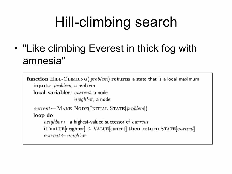
Hill-climbing search

•

"Like climbing Everest in thick fog with amnesia"

Hill-climbing search

•

Problem: depending on initial state, can get stuck in local maxima

Hill-climbing search: 8-queens problem

•

h

= number of pairs of queens that are attacking each other, either directly or indirectly

•

h = 17

for the above state

Hill-climbing search: 8-queens problem

•

A local minimum with h = 1

Simulated annealing search

•

Idea: escape local maxima by allowing some "bad" moves but gradually decrease

their

frequency

Properties of simulated annealing search

•

One can prove: If T

decreases slowly enough, then simulated annealing search will find a

global optimum with probability approaching 1

•

Widely used in VLSI layout, airline scheduling, etc

Local beam search•

Keep track of k

states rather than just one

•

Start with k

randomly generated states

•

At each iteration, all the successors of all k states are generated

•

If any one is a goal state, stop; else select the k best successors from the complete list and

repeat.

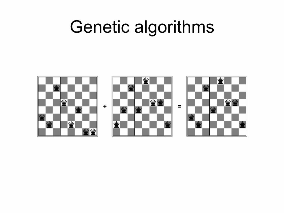
Genetic algorithms•

A successor state is generated by combining two parent

states

•

Start with k

randomly generated states (population

)

•

A state is represented as a string over a finite alphabet (often a string of 0s and 1s)

•

Evaluation function (fitness function). Higher values for better states.

•

Produce the next generation of states by selection, crossover, and mutation

Genetic algorithms

•

Fitness function: number of non-attacking pairs of queens (min = 0, max = 8 ×

7/2 = 28)

•

24/(24+23+20+11) = 31%•

23/(24+23+20+11) = 29% etc

Genetic algorithms