Information Policies andHigher Education Choices

Experimental Evidence from Colombia∗

Leonardo Bonilla†1, Nicolas L. Bottan1, and Andres Ham2

1Department of Economics, University of Illinois2Department of Agricultural and Consumer Economics, University of Illinois

This version: March 2016

Abstract

This paper studies whether providing information on funding opportunities andcollege premiums by degree-college pairs affects higher education decisions in a de-veloping country. We conducted a randomized controlled trial in Bogota, Colombia,on a representative sample of 120 urban public high schools, 60 of which receiveda 35-minute informational talk delivered by local college graduates. Using surveydata linked to administrative records, we analyze student beliefs and evaluate theintervention. Findings show that most students overestimate true college premi-ums and are generally unaware of funding options. The talk does not affect earningbeliefs but improves knowledge of financing programs, especially among the poor.There is no evidence that information disclosure affects post-secondary enrollment.However, students in treated schools who do enroll choose more selective colleges.These positive effects are mostly driven by students from better socioeconomicbackgrounds. We conclude that information policies are ineffective to raise collegeenrollment in contexts with significant academic and financial barriers to entry, butmay potentially affect certain students’ choice of college.

Key words: information, beliefs, higher education, schooling demand, ColombiaJEL Classification: I24, I25, O15

∗We would like to thank the Department of Economics at the University of Illinois for financialsupport. Special thanks are due to Richard Akresh and Martin Perry for their guidance, advice, andencouragement. We are grateful to the Secretary of Education of Bogota for its interest in this projectand authorization to visit the schools, to ICFES and the Ministry of Education for the exit exam dataand enrollment data sets, and to the field work team. Earlier versions benefited from useful commentsby Geoffrey Hewings, Dan Bernhardt, Adam Osman, Rebecca Thornton, Marieke Kleemans, Seema Jay-achandran, Paul Glewwe, Walter McMahon, Julian Cristia, Felipe Barrera-Osorio, Francisco Gallego,Oscar Mitnik, Alejandro Ganimian, Guillermo Cruces, and participants at various seminars and con-ferences. This project was reviewed and approved in advance by the Institutional Review Board forthe protection of human subjects of the University of Illinois at Urbana-Champaign (IRB #13570). Allremaining errors and omissions are our sole responsibility.†lbonill2@illinois.edu (Corresponding author), bottan2@illinois.edu, and hamgonz2@illinois.edu.

Mail: 214 David Kinley Hall, 1407 W. Gregory, Urbana, IL 61801.

1 Introduction

Many developing countries have taken steps to reduce inequality in attendance rates for

primary and secondary education. However, enrollment at post-secondary levels remains

relatively low among the poor, despite its significant returns (McMahon, 2009). While

credit constraints are often cited as the main barrier to attend higher education1, re-

cent research argues that information also plays a key role. In fact, college attendance

decisions are usually based on perceived rather than actual net benefits (Manski, 1993).

Therefore, inaccurate beliefs may lead to sub-optimal schooling choices that have lasting

consequences for lifetime earnings and welfare.

The influence of incorrect beliefs on educational choices has attracted significant atten-

tion because it has a simple and cost-effective solution: providing accurate information.

At basic educational levels, the main concern is low perceived benefits of schooling. Most

papers studying basic education find that students and families tend to underestimate

the returns to education (Nguyen, 2008, Attanasio and Kaufmann, 2009, Jensen, 2010,

Kaufmann, 2014). “Pure” information policies have proven successful in updating these

beliefs. For instance, Jensen (2010) found that reading a short paragraph on the earning

premiums for completing secondary increased educational attainment in the Dominican

Republic by 0.20-0.35 years. Nguyen (2008) finds larger effects in Madagascar when using

role models to deliver information. These treatments may achieve up to 0.24 additional

years of basic schooling per US$100, which is more cost-effective than cash transfers.2

Higher education schooling decisions are more complex, and so is the associated in-

formation problem. On one hand, college represents a major financial investment, and

students usually have limited information regarding its costs and available funding options

(Booij et al., 2012, Loyalka et al., 2013, Dinkelman and Martınez, 2014, McGuigan et al.,

2014, Hoxby and Turner, 2015, Hastings et al., 2015). On the other, higher education

premiums vary dramatically by college and degree, information only recently made avail-

1Previous studies suggests that liquidity constraints not only discourage potential applicants from en-rolling (Manski, 1992, Solis, 2013), but also from applying for and receiving student loans (Kane, 1994,Ellwood and Kane, 2000).2Cost-effectiveness calculations are taken from the Abdul Latif Jameel Poverty Action Lab website, http://www.povertyactionlab.org/policy-lessons/education/improving-student-participation.

2

able to the wider public (Oreopoulos and Petronijevic, 2013, Hastings et al., 2013). While

a number of countries have created websites for this purpose and encouraged students to

visit them3, evidence suggests that they remain largely uninformed. Interestingly, many

studies find that students tend to overestimate the returns to college (Pekkala-Kerr et al.,

2015, McGuigan et al., 2014, Hastings et al., 2015).

This paper conducts a randomized controlled trial (RCT) in which senior high school

students receive information about available funding programs and the premiums to

higher education. We evaluate how providing this information affects their test scores and

enrollment decisions. Our experiment takes place in public schools in Bogota, Colombia.

These schools gather students from low and middle-income families who face severe finan-

cial constraints to attend college and a very small likelihood of admission to affordable

public universities. In addition, since college loans are not backed by the state, funding

institutions require a co-debtor to approve any request for financial assistance. Most of

the students in our sample are unable to fulfill this binding condition.

We randomly selected a citywide representative sample of 120 public schools to par-

ticipate in the study. Half of these schools were given a 35-minute informational talk

delivered by local college graduates. Students were first provided with an overview of the

average premiums associated to attending college compared to finishing high school (and

not finishing). We then introduced the Government website where they could search for

the average starting salaries of college graduates by degree-college pairs, as well as the

probability of finding formal employment by degree. After this, students were briefed on

the admission process and availability of funding programs to cover costs. Almost six

thousand students responded our baseline and follow-up surveys – the latter timed just

before students sat down for the high school exit exam. Survey respondents were later

matched with government administrative records that contain standardized exit exam

scores and college enrollment data (degree and institution of attendance).

Our results indicate the intervention did not affect college enrollment rates. However,

3Some examples are the Observatorio Laboral in Colombia: http://www.graduadoscolombia.edu.co,Mi Futuro in Chile: http://www.mifuturo.cl, and the Observatorio Laboral in Mexico:http://www.observatoriolaboral.gob.mx.

3

students in treated schools that go to college gained admission to more selective insti-

tutions. We find that these individuals increase the likelihood of enrolling in a top-10

college by almost 50% of the mean. This effect is economically significant and potentially

has fairly large implications for future earnings (assuming students’ graduate, of course).

For instance, graduates from top-10 institutions in Colombia have a higher starting salary

compared to other college graduates, about 50% on average.

The limited impact of information in increasing the demand for college may be ex-

plained by its inability to remove financial and academic barriers to entry. Most of our

sample comes from low-income households, whose monthly income is unable to cover the

costs of college education, has below average grades, and cannot fulfill loan requirements.

In fact, students report that the most important obstacles to attend higher education

are that it is unaffordable (64.5%) or difficult to gain admission (32%). Two of our re-

sults further support this interpretation. On the one hand, the information treatment

increased the knowledge of funding programs but did not update earning beliefs. This

is consistent with the fact that students in our sample see costs as the main barrier to

attend college. On the other hand, we find larger effects of the intervention on individuals

from better socioeconomic status, for whom the likelihood of attending college is higher

because these barriers are less binding.

Overall findings are consistent with existing evidence on the effectiveness of “pure”

information policies for higher education. These studies provide information on costs and

funding programs, college premiums, or both. Interventions focusing exclusively on costs

and funding yield mixed results. For instance, Dinkelman and Martınez (2014) increase

high school attendance but have no effect on academic performance in Chile. Loyalka et al.

(2013) increase college enrollment despite not affecting specific college choices in China.

Booij et al. (2012) find no detectable effects on loan take-up in Netherlands. Papers that

only provide information about earning premiums, more in the spirit of Jensen (2010),

tend to be less effective. This is the case of Pekkala-Kerr et al. (2015), who find Finnish

students update their college aspirations but do not change their enrollment choices.

There are three studies similar to ours, where students receive information on premi-

4

ums as well as cost and funding options. Oreopoulos and Dunn (2013) find that Canadian

students raise their college earning expectations. In Avitabile and De Hoyos Navarro

(2015), Mexican students improve their exit exam scores but not their dropout behav-

ior. However, the main limitation of these two papers is that they do not assess effects

on actual enrollment choices. Hastings et al. (2015) focus on a sample of students who

are applying for financial aid in Chile, finding that information on costs and earnings

has no effect on overall enrollment, but does encourage low-income students to choose

higher-earning degrees. It is important to note that our work is different from Hastings

et al. (2015) because we provide information to all students, not only those who apply for

financial aid. This may be a more relevant intervention to Governments considering mass

advertising of different tools to aid students in acquiring more information on college.

This study contributes to two strands of literature. First, it relates to research on

unequal access to higher education. Studying how low-income students make decisions at

the end of high school will shed further light on why so few apply to and ultimately enroll

in college. Second, we add to the burgeoning literature that evaluates information policies

at the post-secondary level, focusing on low-income students from developing countries.

The findings may help understand whether an extensive low-cost information campaign

is useful to attract students to college and if not, why. While our intervention is one of

many possible designs, its implementation and results can potentially inform researchers

and policymakers on what, how, and when information should be provided.

The remainder of this paper is organized as follows. Section 2 provides background on

Colombia’s higher education system. Section 3 describes the experimental framework and

intervention. Section 4 characterizes our data and sample. Section 5 presents the effects

of the information treatment on higher education decisions. Section 6 analyzes what

drives our findings by testing several mechanisms suggested by the literature, including

credit constraints, gender differences, non-cognitive factors, and aspirations. We conclude

in Section 7 by discussing our findings and outlining directions for future research.

5

2 Higher Education in Colombia

There are 327 colleges in Colombia, with 132 located in the Bogota region.4 Of these

132 colleges, 40 are Universities, 23 are public, and 6 are ranked top-10 in the country.5

Degrees are classified in two levels, vocational (2-year) and academic (4-year), that en-

compass 55 fields. Universities supply most of the academic programs, while vocational

degrees are offered at Technical/Technological Institutes. Servicio Nacional de Apren-

dizaje -SENA- is the biggest such institute in Colombia, which is public and completely

free. Universities are not free, but students attending public universities pay tuition under

a progressive system based on family income. While low income households pay between

0.1 and 1.8 minimum wages per semester at top-ranked public universities, the average

tuition fee for private universities in the top-10 is 13.2 minimum wages.6 Scholarships

for low-income students are scarce and only those who achieve the highest scores on the

national exit exam have access to such opportunities.

There are two main funding programs. At the national level, there is the Colom-

bian Public Student Loans Institution (ICETEX), an agency that handles student loans

for vocational, academic, and postgraduate education in Colombia and abroad. This

is the largest student loan program, with 22% of enrolled students during 2013 funded

by this source, and is also the most widely known. Recent reforms, that introduced

zero-interest loans for low-income students, have had large impacts on enrollment and re-

tention (Melguizo et al., 2016). The Secretary of Education of Bogota offers a less-known

funding option for low-income students from the city’s public schools through the Fund

for Higher Education of Bogota (FESBO). The fund has two financing options. The first

targets high achieving students and offers loans for any college or degree choice. The

4The Bogota region includes the city and the following municipalities: Cajica, Chıa, Facatativa, Madrid,Mosquera, and Soacha.5According to the 2012 Higher education exit exams (SABER PRO), the top-10 colleges in Colombiaare (in order): Universidad de los Andes, Universidad Nacional (Bogota), Universidad del Rosario,Universidad Externado, Universidad Icesi (Cali), Universidad Eafit (Medellın), Universidad de la Sabana,Universidad Javeriana, Universidad Nacional (Medellın), and Universidad del Norte (Barranquilla).Universidad Nacional (Bogota and Medellın) are the only public Universities ranked top-10.6Hereafter, all monetary variables will be expressed in monthly minimum wages, a commonly usedmeasure in Colombia. The 2013 monthly minimum wage was 535,600 Colombian Pesos (roughly 288 USDollars). The average excludes medicine, which is usually more expensive than other degrees in privateuniversities.

6

second only provides loans for vocational education. In both cases a fraction of the debt

can be condoned if students complete the degree.

In order to obtain a loan from either funding program, students must fulfill standard

application requirements. However, all credits must be backed by an approved co-debtor,

a restriction that is particularly binding for low-income families. Proposed co-debtors

must pass a credit check and have financial capacity to repay the full debt. In this sense,

Colombia is different from Chile, which provides state-backing for college loans.7

There are significant differences in starting salaries for college graduates between in-

stitutions and degrees. Using official records from the Ministry of Education’s Labor

Observatory, which links individual-level social security records to higher education grad-

uates, we calculate average earnings by college, degree, and field.8 Figure 1 shows the

distribution of earnings for different categories. Notice that the choice of college mat-

ters. In fact, we observe median premiums for private and top-ranked colleges of 0.33

and 1.05 minimum wages, respectively. Degrees are at least as important. While median

earnings for recent graduates with an academic degree are 2.9 minimum wages, individ-

uals with vocational degrees make a median 1.9 minimum wages. Salaries for academic

degree graduates are also much more disperse, reflecting large heterogeneity both within

and between fields. This is partially confirmed by the 0.83 minimum wages premium for

Science, Technology, Engineering, and Mathematics (STEM) degrees.9

In order to characterize the demand for higher education it is worth noting that

Colombia has a large share of private high schools, particularly in urban areas. Private

schools account for 28% of the class of 2013, and 51.4% in Bogota, where higher income

households opt for private education. As shown in the top-left panel of Table 1, 72.6% of

private school students come from middle or high income families (>2 minimum wages),

and 58% have at least one parent who completed higher education. In public schools,

which are completely free, the share of students satisfying these two characteristics drops

7A more detailed description and comparison of the higher education systems of Chile and Colombia canbe found in Gonzalez-Velosa et al. (2015).8We use the 2011 monthly salary for college graduates from 2008-2011 that report non-negative earnings.9Academic degrees from the following fields are classified as STEM: Agronomy, animal sciences, vet-erinary medicine, medicine, bacteriology, biology, physics, mathematics, chemistry, geology, business,accounting, economics, and all engineering.

7

to 29.7% and 15.6%, respectively. One of the reasons why this happens is that private

schools tend to perform better on high school exit exams and have higher college enroll-

ment rates, particularly in selective institutions and degrees.

Test scores reflect significant differences between public and private schools. The na-

tional exit exam, SABER 11, administered by the Colombian Institute for the Promotion

of Higher Education -ICFES- is taken by almost every 11th-grader in public and private

schools, and is required for college admission. Although the application process is com-

pletely decentralized (each institution has its own admission criteria), SABER 11 scores

are heavily weighted by most universities and funding programs. Students are allowed

to take the SABER 11 exam more than once, and it is relatively affordable so it is quite

common to retake if necessary.10 Over the last few years, Bogota’s private schools have

consistently scored 0.76 SD above the city’s public schools as Table 1 shows.

Less than half the students who graduate from high school enroll in college, and the

odds are significantly smaller for public school students. The National Information Sys-

tem for Higher Education -SNIES- matches SABER 11 information to higher education

administrative records for all institutions, allowing to track how many students enroll.

Our estimates based on SNIES indicate that only 46.9% of the students that graduated in

Bogota during 2013 enrolled in higher education during 2014. Moreover, private schools

perform much better, since their students have consistently higher probabilities of en-

rolling (57.1%) and doing so in a private (42.4%) or a top-10 (16%) college. They are

also more likely to choose academic and STEM degrees as Table 2 denotes.

In summary, Bogota has a very heterogeneous higher education system that trans-

lates into large wage premiums for selective colleges and degrees. However, there are

significant financial and academic barriers to entry for low-income and low-achieving stu-

dents. On the demand side, Bogota’s higher income families opt for private schools that

have significantly higher exit exam scores and better placement in selective colleges and

degrees. This paper studies public schools in order to focus on the group that is most

disadvantaged in terms of access to higher education.

10The exam fee is roughly equivalent to US$17 for students taking the SABER 11 for the first time and$21 otherwise.

8

3 Experimental Setting

3.1 Randomization

In order to study the effects of information on higher education decisions, we conducted

a randomized control trial in Bogota, Colombia. Our population of interest were public

high school students enrolled in their senior year. We focused on public schools since

they have significantly lower college enrollment rates, particularly when it comes to se-

lective institutions and degrees. A representative sample of 120 public school-shifts were

randomly selected out of the 570 that offer an academic track.11 These institutions are

all mixed-sex, urban, high schools with at least 20 senior high school students enrolled in

the 2012 academic year. Half of the 120 high schools were randomly assigned to receive

an informational talk detailing college premiums by degree-college pairs and discussing

funding opportunities, while the remaining institutions served as our comparison group.

While conducting our surveys at schools, we only interviewed students from two class-

rooms. These were selected at random if there were more than two classrooms at the

senior level. Otherwise, we surveyed all students in attendance that day. In Colombia,

the public school year often begins in February and ends in December. The timing of

our intervention is summarized in Figure 2. Fieldwork for the baseline survey and the

intervention took place during March 2013. The follow-up survey was conducted in Au-

gust 2013, just before students took the SABER 11 exam. Our sample of schools covers

a large extent of the city and most urban neighborhoods in Bogota, with treatment and

control schools being relatively spread out as Figure 3 shows.

3.2 The Intervention

During our baseline visits in March we first collected self-administered surveys. After

all surveys were collected, students in treatment schools were given a 35-minute presen-

11Most public high schools in Bogota have two shifts: morning and afternoon. Each shift has differentstudents and most importantly, different teachers and staff. Hence, each school-shift may be consideredas an independent educational institution. In what follows, we refer to school-shifts as schools.

9

tation delivered by young local Colombian college graduates.12 The talk described the

relationship between higher education and earnings, presented the most relevant funding

programs to finance post-secondary studies, and emphasized the importance of exit exam

scores for admission committees.

The talk began by describing statistics on the average monthly earnings of individuals

with incomplete and complete secondary, then comparing these values to the expected

salaries of individuals who completed a higher education degree (differentiating by voca-

tional and academic).13 We then introduced students to two websites where they could

find very detailed information on the labor market outcomes of recent higher education

graduates, including average earnings by degree-college pairs and the probability of ob-

taining formal employment by career.14 Additionally, we showed how the different search

tools on the websites worked using some examples.

The second part of the talk focused on two funding programs: ICETEX and FESBO.

For each program, we provided basic information regarding benefits, application require-

ments, and deadlines. Students were encouraged to visit the websites of each program

for more information. We emphasized the fact that college education can be affordable,

even if they choose a relatively expensive university.

The last portion of the talk focused on the importance of the high school exit exam

(SABER 11). We insisted on the fact that this test is a determinant factor for admission

decisions in most colleges, and that higher scores also increase the possibility of receiving

funding. Students were allowed some time for questions and we gave out a one-page

handout summarizing the main points of the talk and containing all the relevant links to

the websites described during the talk.15

12We opted for local college graduates based on findings in Nguyen (2008), where information providedby local role models yielded higher effects.13Reference earnings for incomplete and complete secondary are 0.85 and 1.07 minimum wages, respec-tively and were estimated using 2011 household surveys.14The websites are: http://www.graduadoscolombia.edu.co/ and http://www.finanzaspersonales.

com.co/calculadoras/articulo/salarios-profesion-para-graduados/45541. They present LaborObservatory information of individuals who graduated from higher education in a user-friendly way.15The original and translated copy of this handout may be found in the Appendix.

10

4 Data and Estimation Strategy

4.1 Data

The baseline survey collected information on 6,636 students in 116 schools.16 The ques-

tionnaire inquired about individual demographic characteristics, family background, so-

cioeconomic status, educational background, aspirations, current employment, future

work perspectives, and attitudes towards risk. The follow-up survey was completed by

6,141 students in the same 116 schools.17 The questionnaire followed up on some baseline

questions, mainly educational and employment aspirations. It also added modules on

students’ household environment. In what follows, we refer to the survey data as the

Bogota Higher Education and Labor Perspectives Survey (BHELPS).

The survey data are further augmented by matching students in our sample to two

administrative sources: the ICFES (Colombian Institute for the Promotion of Higher Ed-

ucation) and SNIES (National Information System for Higher Education). ICFES records

contain scores for the high school exit exam (for the 8 different subjects and the overall

score), as well as information on date of birth, gender, parents’ education, and family

income. We use the administrative records for these variables when they are missing in

the BHELPS survey. The SNIES higher education enrollment records for 2014 provide

evidence on whether students in our sample enrolled in a higher education program, iden-

tifying both the institution and degree. The matching rates for ICFES and SNIES to

the baseline sample are quite high: 95.3% and 95%. There are no significant differences

between matched and unmatched students and the rates are similar across treatment and

control groups.18 We present results for three samples: i) all students observed in the

follow-up BHELPS, ii) students observed in the baseline BHELPS successfully matched

to the administrative data, and iii) individuals observed in the baseline and follow-up

rounds of the BHELPS that are matched to each source of administrative data.

16Despite numerous attempts, we were unable to visit four schools. These corresponded to 3 treatmentschools and 1 control school. However, the inability to interview these students does not seem to gen-erate issues that affect randomization nor representativity as our descriptive statistics and balance testspresented below reveal.17Attrition between baseline and follow-up waves was 7.5%, mainly due to absences on survey days.18See Table A.1 in the Appendix for attrition diagnostics.

11

4.2 Sample Representativity and Characteristics

Our sample, which includes approximately 20% of the city’s public high schools, is rep-

resentative of the target population though slightly over-sampled morning-shift schools.

Table 1 summarizes individual and school-level characteristics for all private and public

schools, as well as surveyed students in the BHELPS. In Table 3, we present baseline

characteristics for students in control and treatment groups, as well as the p-value for the

differences (clustering standard errors at the school level). Both groups look very similar

on their observable characteristics, suggesting that our randomization was successful.

On average, students are almost 18 years old when they graduate (measured in De-

cember 31, 2013) and most were born in Bogota (84.7%). Almost a quarter of students

have repeated at least one grade. Around 15% of students in the treatment group have

at least one parent that completed college, around 2 points lower than the control group,

though not statistically different. Students in treatment and control groups look almost

identical in terms of family income, where 31% report income over 2 minimum wages.

Since most high-income families opt for private education, we will classify students in

public schools with a family income higher than 2 minimum wages as middle-income.

Approximately 71% of students in the control group have internet at home, while inter-

net access is almost 4 points lower for treatment students and the difference is barely

statistically significant at the 10% level.

We asked students in the follow-up survey what they believed to be the most signifi-

cant barriers to enroll in college. The majority responded that college was unaffordable

(64.5%), followed by 32% who claimed that obtaining admission was the largest obsta-

cle. This is consistent with the fact that private education is expensive and affordable

public universities are very selective. While only 31% of our sample reports monthly

family income above 2 minimum wages, college tuition for a semester may rise to 13.2

minimum wages at private top-10 institutions, which is equivalent to 2.2 minimum wages

per month. As for progressively-priced public universities (that may cost as little as 0.1

minimum wages) admission rates are fairly low. While 40% of the students in our sample

wanted to enroll in the National University in the baseline survey, less than 1% made

12

it. These students might also face bureaucratic barriers from funding institutions. As

mentioned before, most available programs require a co-debtor to back college loans.

Given that risk aversion has been found to play an important role for human capital

accumulation decisions (Heckman, 2007), students were asked to play two different games

in the baseline.19 The resulting classification indicated that 85% of our sample was risk

averse. To measure academic self-concept, we ask students to rank themselves relative

to the rest of the class on a Likert-scale from 1-10 where the latter is the highest value.

As a measure of self-efficacy, students rated how often they achieved their proposed goals

(from 1 to 10, where 1 is never and 10 is always). Individuals above the median response

are classified as high academic self-concept and self-efficacy, while those below constitute

the low group. We also asked their perceived probability of enrollment in college the

following year. Almost 85% reported in the baseline survey that they were likely to enroll

but only 19.4% were certain of attending some post-secondary institution.

Treatment and control groups look very similar in school characteristics. Using ad-

ministrative data from 2010-2012, we find on average that over 90 students per school sit

for the SABER 11 exam each year. Additionally, previous cohorts performed similarly

across groups. More than half the schools are morning shift and over 95% of them have a

computer lab. A joint-test for balance rejects that individual and school-level attributes

explain the likelihood of attending a treatment school, with a p-value of 0.680.

4.3 Estimation Strategy

Given the random assignment of the treatment, we quantify the effect of providing infor-

mation on our main outcomes (e.g. college enrollment, SABER 11 exam scores, etc.) by

estimating a cross-sectional regression, where outcomes in period t = 1 are explained by

baseline treatment status and attributes:

yis,t=1 = α + βTs + θXis,t=0 + uis,t=1 (1)

19Students face the following hypothetical scenario: They were just hired for a new short-term job andcan choose between a fixed salary or a lottery in which earnings are determined by a coin flip. By varyingthe optimistic scenario payment, we classify students in a scale from 1 to 4 where 1 is extremely riskaverse and 4 is risk loving. We consider a student risk averse if they are classified 1 or 2.

13

where yis,t=1 is the studied outcome for student i attending school s at the follow-up, t = 1.

We include an intercept, α, and control for baseline student-level attributes (male, age,

age squared, family income, and parental education) and school characteristics (average

score on exit exam in previous years, has computer lab, shift indicators, and school size)

with Xis,t=0. Our coefficient of interest is β, which captures the average effect of the

informational treatment. uis,t+1 is a mean-zero error term assumed to be uncorrelated

with the treatment indicator since it was randomly assigned. Equation (1) is estimated

by Ordinary Least Squares (OLS)20, clustering standard errors at the school-level. Given

that the actual take up of the information depends on the level of attention placed by

students, β would capture the intent-to-treat rather than the average treatment effect of

acquiring new information on degree-college premiums and funding options.

When studying the potential mechanisms driving our main results, we take advantage

that some outcomes are available for both the baseline and follow-up BHELPS surveys. In

these cases, we employ two additional specifications. First, we estimate Equation (1), but

include the outcome at the baseline as an additional explanatory variable. This approach

could potentially provide additional power. Second, we estimate a difference-in-differences

specification; defining a binary variable, Post, that equals one after information exposure

and zero otherwise:

yist = αPost+ β(Ts × Post) + µi + uist (2)

where α estimates the change in the outcome over time and µi is a student-specific

effect that controls for all time-invariant characteristics (observed and unobserved) in our

sample. Again, β is our coefficient of interest, which measures the average effect of the

information treatment on the studied outcome. Standard errors are also clustered at the

school-level. Note that the modified Equation (1) and Equation (2) can only be estimated

for outcomes obtained in the BHELPS surveys and not from administrative data (i.e. test

scores and enrollment outcomes).

20We also estimate Probit regressions but the main results are largely unchanged. We therefore chooseto report only OLS estimates.

14

5 Results

This section studies the effect of information disclosure on higher education outcomes.

Since information should first affect beliefs, then decisions in high school, and ultimately

college enrollment, the findings are presented in that order.

5.1 Beliefs

Our measures of student perceptions include knowledge about funding programs and

beliefs about labor market premiums. Knowledge is measured using binary variables

that denote awareness of funding institutions (ICETEX and FESBO).21 Earning beliefs

are measured by the error between perceived and actual premiums for vocational and

academic degrees relative to completing high school.22

Baseline statistics for knowledge and beliefs are presented in Table 4. Almost 70% of

students express familiarity with ICETEX and 18% know FESBO, with both treatment

and control groups reflecting similar baseline knowledge. These patterns illustrate that

students remain largely unaware of the existence of certain funding programs. On aver-

age, public high school students in Bogota overestimate college premiums. Approximately

87.6% overestimate the premiums to vocational degrees and 89.1% for academic degrees.

Reported errors for vocational and academic degrees are 69.6% and 118% larger on av-

erage. These results are consistent with findings for the same population in Colombia

(Gamboa and Rodrıguez, 2014) and other countries (Pekkala-Kerr et al., 2015, McGuigan

et al., 2014, Hastings et al., 2015).

In addition to overestimating the average premiums to college education, students

show sizable variation in their beliefs. Figure 4 plots the distribution of errors for voca-

tional and academic premiums. Individuals overestimate the associated benefits of voca-

tional degrees, but most of them are not far from the correct belief. 76.3% are within

21While desirable, we were unable to collect a measure that captures the degree of knowledge aboutfunding programs.22Similar to Hastings et al. (2015), we calculate errors by estimating the difference between perceived andactual premiums and then dividing by the actual premium. That is, if πj denotes the wage premium andj = {actual, perceived}, then our measures are (πperceived − πactual)/πactual. Results are similar whenusing different measures.

15

one standard deviation of the true premiums. Earning beliefs for academic degrees are

more disperse: 60.1% of surveyed students have errors of one standard deviation, 29.2%

between one and three standard deviations, and 10.7% more than three standard devia-

tions. Students are therefore more misinformed about the average premiums for academic

degrees than vocational careers.23

Are students who overestimate different than those who underestimate? Table 5

presents student and school characteristics based on the direction of their baseline beliefs:

below the true premium or above it. There are no differences across students in treatment

and control schools, as expected. Younger students seem to overestimate college premiums

for both vocational and academic degrees. Interestingly, low income students tend to

underestimate the monetary benefits to college education while higher income individuals

overestimate. There is also evidence that repeaters, risk averse, and more confident

students are more likely to overestimate college premiums relative to their counterparts.

The effects of information on knowledge and beliefs are presented in Table 6. Panels

A and B report cross-section estimates on two samples: all students observed in the

follow-up BHELPS and students observed in both BHELPS rounds. Panel C presents

difference-in-differences results with individual fixed-effects for the second sample. We

find that the treatment increases knowledge of the largest funding program, ICETEX.

Students in treated schools increase their average awareness of this institution by 3.8

percentage points, or 6.6% of the mean. The impact is larger for students observed in both

rounds, with cross-section and difference-in-difference effects of 4.7 and 4.6 percentage

points, respectively. There are no statistically significant effects on knowledge of FESBO

or perceived premiums.

We find that students are acquiring more information over time, independently from

our intervention. The coefficient for the follow-up period (Post) in Panel C is positive and

significant for both funding programs. Likewise, all individuals significantly reduce the

degree to which they were overestimating college premiums. This reflects that students

23Jensen (2010) suggests that noisier beliefs for higher education may be due to college being a rareoutcome. In our sample, less than 18% of the students have parents who completed higher education.These students have slightly more accurate beliefs for vocational degrees, but not for academic degreescompared to those whose parents have not completed higher education.

16

in our sample gain further knowledge about higher education during their senior year.

One potential reason we do not find that students in treated schools corrected their

beliefs at a faster rate than control students could be due to opposing effects: students

who were initially overestimating before the intervention update downwards and those

that were underestimating update upwards. We test for this possibility by estimating

separate regressions for each group defined at baseline in Table 7. Similar to the average

effects, individuals do correct their beliefs in the appropriate direction, but not because of

the information treatment. Once again, students acquire information over time on their

own, pushing them closer to the actual earning premiums.

As an additional robustness test, we change the reference values for earning beliefs.

In all previous estimates, we compared students’ perceptions to the average vocational

and academic premiums with respect to high school. Perhaps students used their own

expectations as a reference instead of those for an average individual. In the baseline

BHELPS, we asked students to tell us the degree, college, and field they aspired. Using

the records from the Labor Observatory on starting salaries for college graduates, we

calculated two measures of expected earnings for each student: i) by degree and field,

and ii) by degree and college. The same analysis from Tables 6 and 7 confirms that the

treatment did not affect premium beliefs (results are shown in Table A.2 in the Appendix).

5.2 Test scores

As previously mentioned, academic performance plays a central role in college admis-

sions in Colombia. The informational talk could have affected effort in high school by

increasing the desirability or attainability of a post-secondary degree. We measure stu-

dent performance using test scores from the national high school exit exams (SABER 11)

that was taken approximately five months after our intervention. In particular, we focus

on the overall score and the two most important subjects: mathematics and language.24

All scores are standardized with mean zero and standard deviation of one with respect

to the control group for ease of comparison.

24The overall score is computed using the official weights: mathematics (3), language (3), social sciences(2), biology (1), physics (1), chemistry (1) and philosophy (1).

17

Table 8 presents the average effects of information on test scores for all students

matched to administrative records (Panel A), and two more restricted samples of students:

those observed in the baseline BHELPS that were successfully matched and individuals

observed in both baseline and follow-up who were matched (Panels B and C). While the

estimated coefficients are consistently larger for mathematics, we do not find statistically

significant effects of the treatment on test scores for any sample.

We test for differential effects along the score distribution using quantile regressions.

Figure 5 presents quantile treatment effects and their corresponding 90% confidence in-

terval for test scores on mathematics and language. There is suggestive evidence of some

positive and significant effects on students at the lower end of the distribution in math.

The treatment induced students in the lower 20th percentile to perform nearly a tenth

of a standard deviation better in mathematics. In turn, only students at the highest

percentiles performed better on language. Nevertheless, the average estimates suggest

that information had no overall effect on test scores, and small quantile effects.

5.3 College Enrollment

We are able to track students who enrolled in higher education after graduation, and

may further characterize their college and degree of choice. The enrollment rate for

a post-secondary degree (academic or vocational) in our sample is 44.4%, with around

34.8% enrolled in a vocational program. Less than 10% of the students enroll in academic

degrees, very few in top-ranked colleges (1%), and STEM degrees (4.9%).

Table 9 presents treatment effect estimates on higher education enrollment for the

same three samples used in Table 8. We find that the effect of information on the

probability of enrolling in any post-secondary program is not statistically distinguishable

from zero. However, there is a significant increase in the probability of enrolling in a top-

10 college. Effects range from 0.4 to 0.6 percentage points depending on the sample. This

impact, though small in magnitude, is also economically significant. In fact, it represents

an increase of approximately 50% with respect to the control group average. Estimated

effects on the other three intensive margin outcomes are also positive but not statistically

18

significant.

Our results are consistent with previous literature. Among “pure” information treat-

ments, most studies find no effect of disclosing information on higher education enrollment

(Booij et al., 2012, Fryer, 2013, Oreopoulos and Dunn, 2013, Pekkala-Kerr et al., 2015,

McGuigan et al., 2014, Dinkelman and Martınez, 2014, Wiswall and Zafar, 2015). Our

intensive margin effects are consistent with those of interventions focusing on students

who are already applying to college and have a high probability of enrollment (Hoxby and

Turner, 2013, Hastings et al., 2015). In the long run, opting for a top-10 college may have

important implications on future earnings (conditional on graduating). Recall from Fig-

ure 1 that students who graduate from a top-10 college in Colombia earn approximately

50% more than non-top college students (1 minimum wage more on average). Therefore,

while providing information may not lead more individuals to attend college, it does seem

to affect what colleges are chosen by those who do enroll.

6 Mechanisms

The effects of providing “pure” information appear to have been modest overall. On the

one hand, students update their knowledge on funding programs but not their earning

beliefs. On the other hand, we observe no improvement on college enrollment but a higher

likelihood of admission to top-10 colleges. In this section we explore potential mechanisms

that help interpret these results.

Our analysis highlights the role of credit constraints, gender differences, non-cognitive

factors, and aspirations. We have already discussed that the main barrier to college atten-

dance for low income students in Colombia are its high costs. Additionally, there remain

considerable gender differences in higher education choices and labor market outcomes

(Goldin et al., 2006). In part, this may reflect gender-specific traits or preferences that

affect boys and girls differentially.25 Non-cognitive factors also play an important role

in determining human capital accumulation and academic success (Heckman and Rubin-

25For instance, there is evidence that when given the option, women shy away from competition (Niederleand Vesterlund, 2007), perform less well in competitive environments (Gneezy et al., 2003), and self-selectinto less competitive or lower earning careers (Buser et al., 2014).

19

stein, 2001). We assess potential heterogeneity by two non-cognitive dimensions: risk

aversion (Belzil and Hansen, 2004, Belzil and Leonardi, 2007, Heckman, 2007), as well

as self-concept and self-efficacy (Benabou and Tirole, 2002, Heckman et al., 2006). Last,

aspirations may keep poor children from pursuing more ambitious goals or induce frus-

tration because of the difficulties in achieving their them (Appadurai, 2004, Ray, 2006,

Heifetz and Minelli, 2014, Genicot and Ray, 2014, Dalton et al., 2016).

6.1 Credit Constraints

To evaluate the extent to which credit constraints could explain our results, we explore

the heterogeneity of treatment effects by estimating fully interacted versions of Equation

(1) by income groups. Table 10 presents separate coefficients for each grouping (low and

middle) for our main outcomes. It also includes the p-value for a Wald test that these

coefficients are equal. For parsimony, we focus on the sample of students observed in the

baseline that are matched to the later rounds of survey data and administrative records.26

In column (1) we find that only students from low-income families learn about ICE-

TEX – the main funding institute. While the estimated effect on middle-income students

is not statistically significant, low-income students increased their knowledge of ICETEX

by about 5.4 percentage points. This effect is statistically different from the effect on

middle-income students. This likely reflects a catching-up: students from higher income

families report significantly higher knowledge of funding programs in the baseline survey.

We do not find any statistically relevant effects or differences between income levels for all

other knowledge or belief outcomes. Overall, students appear to have valued information

on financing more than that of earnings, suggesting that credit constraints are indeed a

primary concern for most of the students in our sample.

Columns (2) to (4) present heterogeneous effects of the intervention by income level

on test scores. Unlike knowledge of ICETEX, positive effects are driven by students from

middle-income families, with an increase in mathematics and language scores of 8.2% and

7.1% standard deviations, respectively.

26Appendix Table A.3 presents results using individuals observed in both rounds of the BHELPS andmatched to each source of administrative data. Those findings are unchanged from those discussed here.

20

Heterogeneous effects by family income on enrollment outcomes are presented in

columns (5) to (9). As with the average estimates, we find no significant effects. How-

ever, students’ intensive margin decisions respond differently to information depending on

their income category. First, entry to top-10 colleges is dominated by middle-income stu-

dents. The estimated effect is 1.2 percentage points and statistically different from that

of low-income students. Second, poorer students increase their probability of enrolling

in a private college, with an estimated coefficient of 2.1 percentage points. However, the

difference with respect to middle-income students is not statistically significant.

In general, we find that most of the positive effects of the intervention were on the

students from middle-income families in our sample. This further supports that providing

information may have limited effects on higher education demand when such interventions

do not eliminate the main barriers to entry. In the Colombian case these are twofold:

sizable credit constraints and low probabilities of admission to affordable institutions.

Since most of the higher-income students are already aware of available funding options,

it seems plausible that information provides them with additional motivation to perform

better on the exit exam and therefore attend more selective colleges.27

6.2 Gender differences

In Panel C of Table 10, we present heterogeneous effects by gender. At baseline, boys

had significantly lower knowledge of ICETEX than girls. The treatment appears to have

bridged this gap as suggested by the positive and statistically significant effect on males

and no statistically distinguishable effect for females. At the same time, there is suggestive

evidence that males increased their performance on mathematics by 0.07 of a standard

deviation. However, this effect is not statistically different to the effect for females.

Evaluating the heterogeneous effects on enrollment outcomes in columns (5) to (9),

we find suggestive evidence that the information treatment increased college enrollment,

27In the Appendix, we also consider heterogeneous effects by the direction of errors in baseline earningexpectations. Our results showed that poorer students underestimate college premiums while richerchildren overestimate. Findings are shown in Table A.4 and are similar to those using income groups.While information has slightly larger positive effects on those who underestimate, these differences arenot statistically significant.

21

private, and top-10 college admission for boys, but no statistically significant effects for

girls. Nevertheless, we cannot reject the null hypothesis that the effects between males

and females are the same (although overall enrollment is borderline insignificant at the

10% level). Even though each effect in itself is at best suggestive, these results are largely

consistent with existing studies that find that males are encouraged (maybe driven by

overconfidence) to pursue more competitive degrees (Buser et al., 2014).

6.3 Other factors

We now explore additional factors that might influence the impact of the information

treatment. We focus on non-cognitive factors that have been identified as key determi-

nants of education choices and student aspirations.28

Panel A of Table 11 explores differences by risk aversion. Risk loving students increase

their probability of enrolling in academic and STEM degrees, with estimated effects of 3.1

and 3.8 percentage points. Differences with respect to risk averse students are significant

for STEM degrees but not academic. This suggests that information may resonate more

with students who take more risks. It is important to note that one shortcoming of this

measure is that pursuing higher education is likely an intra-household decision taken by

a student and his/her parents. Unfortunately, we do not count with measures of parental

risk aversion but this would be an interesting avenue for future studies to address.

We also assess the role of self-confidence and self-efficacy using three proxies. The first,

academic self-concept, measures whether a student believes they are above average in aca-

demic terms (Panel B of Table 11). We find no significant differences by this classification.

The second, student self-efficacy, measures whether students are more likely to achieve

their goals (Panel C of Table 11). We find that highly self-efficacious students improve

both mathematics and language test scores, and increase their probabilities of enrolling

in academic and STEM degrees. Nevertheless, only the difference in language scores are

statistically significant. The third, perceived likelihood of enrollment, reflects not only

students’ self-concept and self-efficacy, but also accounts for the financial constraints they

28Appendix Table A.5 presents largely similar results for the sample of individuals observed in both roundsof the BHELPS and matched to each source of administrative data.

22

foresee (Panel D of 11). Students with low probabilities of enrollment learn more about

financial programs, with an estimated effect of 10.2 percentage points. However, this does

not lead to higher enrollment rates or more selective choices. On the contrary, enrollment

effects are concentrated on students with higher perceived probability of enrolling. For

top-10 colleges, the difference between groups is statistically significant.

Finally, we examine whether information affects student aspirations. We exploit a

question in both BHELPS waves that asks students what college and degree they would

like to attend.29 Because students absorb the information about financing institutions,

this could affect their aspirations (whether they want to enroll in a post-secondary pro-

gram or what type of degree they desire). Results for these outcomes are presented in

Table 12. Findings show no effect of information on any of the aspiration measures. This

suggests that intensive margin effects on enrollment are not driven by changes in student

aspirations.

7 Conclusion

This paper analyzes whether providing information on funding opportunities and college

premiums by degree-college pairs affects higher education decisions in Bogota, Colombia.

We conduct a randomized controlled trial on a representative sample of 120 urban public

high schools, half of which received an informational talk. Using survey data linked to

administrative records, we analyze student beliefs and evaluate the intervention. We

find that most students overestimate true college premiums and are generally unaware

of funding options. The talk does not affect earning beliefs but improves knowledge of

financing programs, especially among the poor. There is no evidence that our treatment

affects post-secondary enrollment. However, students in treated schools who do enroll

choose more selective colleges. These positive effects are mostly driven by students from

better socioeconomic backgrounds.

Our findings confirm that misinformation is a problem among potential college en-

trants since they tend to overestimate its benefits and are mostly unaware of its costs.

29Descriptive and balance statistics for the aspiration outcomes may be found in Appendix Table A.6.

23

However, this is not the main deterrent for attending college. The existence of significant

academic and financial barriers to college entry in Colombia might limit the influence

of better information because low-income students believe the system limits upward mo-

bility. In fact, we find larger effects of the intervention on middle-income individuals,

for whom the likelihood of attending college is higher since constraints are less binding.

Moreover, our treatment increased the knowledge of funding programs but did not up-

date earning beliefs. This is consistent with most students in our sample believing that

costs are the main barriers to higher education. We conclude that providing information

cannot single-handedly increase higher education enrollment among low-income students

in this context. It takes more comprehensive measures, such as zero-interest rates loans

(Melguizo et al., 2016), to achieve substantial improvements in this respect.

Despite the inability to attract more low-income students into college, providing infor-

mation has some positive effects on college choices for those who enrolled. These results

are particularly interesting since we targeted a wider population than other papers, such

as Hastings et al. (2015) and Hoxby and Turner (2013), and yet found similar results in

the intensive margin. Given the low-cost of “pure” information interventions, policymak-

ers may therefore consider less targeted policies to orient students in their college choices,

even if only a fraction of them is expected to benefit from the additional information.

How and when to provide information is an interesting direction for future research.

Our intervention is one of many possible designs in this respect. For instance, while we

provided average college premiums, future studies could present the entire distribution

of earnings in a simple and intuitive manner. Likewise, disclosing more detailed cost

data may be useful. The timing of information policies, especially for higher education

choices, is also highly relevant. Additionally, whether these interventions should target

students, parents, or both is an open-ended question. Our results indicate that providing

information to students in the final year of high school is mostly ineffective since it does

not eliminate existing barriers to entry. However, earlier interventions of the benefits and

costs of education to students and their parents may affect household behavior so that by

the time children apply to college, both academic and financial barriers are less binding.

24

References

Appadurai, A. (2004). The capacity to aspire: Culture and the terms of recognition. InRao, V. and Walton, M., editors, Culture and Public Action. Stanford University Press.

Attanasio, O. and Kaufmann, K. (2009). Educational Choices, Subjective Expectations,and Credit Constraints. NBER Working Papers 15087, National Bureau of EconomicResearch, Inc.

Avitabile, C. and De Hoyos Navarro, R. E. (2015). The Heterogeneous Effect of Informa-tion on Student Performance: Evidence from a Randomized Control Trial in Mexico.World Bank Policy Research Working Paper, (7422).

Belzil, C. and Hansen, J. (2004). Earnings dispersion, risk aversion and education. InPolachek, S. W., editor, Accounting for Worker Well-Being (Research in Labor Eco-nomics, Volume 23), pages 335–358. Emerald Group Publishing Limited.

Belzil, C. and Leonardi, M. (2007). Can risk aversion explain schooling attainments?Evidence from Italy. Labour Economics, 14(6):957–970.

Benabou, R. and Tirole, J. (2002). Self-confidence and personal motivation. QuarterlyJournal of Economics, pages 871–915.

Booij, A. S., Leuven, E., and Oosterbeek, H. (2012). The role of information in thetake-up of student loans. Economics of Education Review, 31(1):33–44.

Buser, T., Niederle, M., and Oosterbeek, H. (2014). Gender, competitiveness, and careerchoices. The Quarterly Journal of Economics.

Dalton, P. S., Ghosal, S., and Mani, A. (2016). Poverty and aspirations failure. TheEconomic Journal, 126(590):165–188.

Dinkelman, T. and Martınez, C. (2014). Investing in Schooling In Chile: The Role ofInformation about Financial Aid for Higher Education. The Review of Economics andStatistics, 96(2):244–257.

Ellwood, D. and Kane, T. (2000). Who is getting a college education? Family backgroundand the growing gaps in enrollment. In Danziger, S. and Waldfogel, J., editors, Securingthe Future, pages 283–324. New York: Russell Sage Foundation.

Fryer, R. G. (2013). Information and Student Achievement: Evidence from a Cellu-lar Phone Experiment. NBER Working Papers 19113, National Bureau of EconomicResearch, Inc.

Gamboa, L. F. and Rodrıguez, P. A. (2014). Do Colombian students underestimate highereducation returns? Working Paper 164. Universidad del Rosario.

Genicot, G. and Ray, D. (2014). Aspirations and inequality. Working Paper 19976,National Bureau of Economic Research.

Gneezy, U., Niederle, M., and Rustichini, A. (2003). Performance in competitive environ-ments: Gender differences. The Quarterly Journal of Economics, 118(3):1049–1074.

25

Goldin, C., Katz, L. F., and Kuziemko, I. (2006). The Homecoming of American CollegeWomen: The Reversal of the Gender Gap in College. Journal of Economic Perspectives,20:133–156.

Gonzalez-Velosa, C., Rucci, G., Sarzosa, M., and Urzua, S. (2015). Returns to Higher Ed-ucation in Chile and Colombia. Technical report, Inter-American Development Bank.

Hastings, J., Neilson, C. A., and Zimmerman, S. D. (2015). The Effects of EarningsDisclosure on College Enrollment Decisions. NBER Working Papers 21300, NationalBureau of Economic Research, Inc.

Hastings, J. S., Neilson, C. A., and Zimmerman, S. D. (2013). Are some degrees worthmore than others? Evidence from college admission cutoffs in Chile. Technical report,National Bureau of Economic Research.

Heckman, J. J. (2007). The economics, technology, and neuroscience of human capabilityformation. Proceedings of the national Academy of Sciences, 104(33):13250–13255.

Heckman, J. J. and Rubinstein, Y. (2001). The importance of noncognitive skills: Lessonsfrom the GED testing program. American Economic Review, 91(2):145–149.

Heckman, J. J., Stixrud, J., and Urzua, S. (2006). The effects of cognitive and noncog-nitive abilities on labor market outcomes and social behavior. Journal of Labor Eco-nomics, 24(3):411–482.

Heifetz, A. and Minelli, E. (2014). Aspiration traps. The B.E. Journal of TheoreticalEconomics, 15(2):125–142.

Hoxby, C. and Turner, S. (2013). Expanding college opportunities for high-achieving, lowincome students. Stanford Institute for Economic Policy Research Discussion Paper,(12-014).

Hoxby, C. and Turner, S. (2015). What high-achieving low-income students know aboutcollege. Technical report, National Bureau of Economic Research.

Jensen, R. (2010). The (Perceived) returns to education and the demand for schooling.The Quarterly Journal of Economics, 125(2):515–548.

Kane, T. (1994). College entry by blacks since 1970: The role of college costs, familybackground, and the returns to education. Journal of Political Economy, 102(5):878–911.

Kaufmann, K. M. (2014). Understanding the income gradient in college attendancein mexico: The role of heterogeneity in expected returns. Quantitative Economics,5(3):583–630.

Loyalka, P., Song, Y., Wei, J., Zhong, W., and Rozelle, S. (2013). Information, collegedecisions and financial aid: Evidence from a cluster-randomized controlled trial inchina. Economics of Education Review, 36:26–40.

Manski, C. (1992). Income and higher education. Focus, 14(3):14–19.

26

Manski, C. F. (1993). Adolescent econometricians: How do youth infer the returnsto schooling? In Studies of supply and demand in higher education, pages 43–60.University of Chicago Press.

McGuigan, M., McNally, S., and Wyness, G. (2014). Student awareness of costs and ben-efits of educational decisions: Effects of an information campaign and media exposure.Technical report, Department of Quantitative Social Science-Institute of Education,University of London.

McMahon, W. (2009). Higher Learning, Greater Good: The Private and Social Benefitsof Higher Education. Johns Hopkins University Press.

Melguizo, T., Sanchez, F., and Velasco, T. (2016). Credit for Low-Income Students andAccess to and Academic Performance in Higher Education in Colombia: A RegressionDiscontinuity Approach. World Development, 80:61–77.

Nguyen, T. (2008). Information, role models and perceived returns to education: Exper-imental evidence from Madagascar. Unpublished manuscript.

Niederle, M. and Vesterlund, L. (2007). Do women shy away from competition? do mencompete too much? The Quarterly Journal of Economics, 122(3):1067–1101.

Oreopoulos, P. and Dunn, R. (2013). Information and College Access: Evidence from aRandomized Field Experiment. Scandinavian Journal of Economics, 115(1):3–26.

Oreopoulos, P. and Petronijevic, U. (2013). Making college worth it: A review of researchon the returns to higher education. Technical report, National Bureau of EconomicResearch.

Pekkala-Kerr, S., Pekkarinen, T., Sarvimaki, M., and Uusitalo, R. (2015). Post-SecondaryEducation and Information on Labor Market Prospects: A Randomized Field Experi-ment. IZA Discussion Papers 9372, Institute for the Study of Labor (IZA).

Ray, D. (2006). Aspirations, poverty, and economic change. Understanding poverty, pages409–21.

Solis, A. (2013). Credit Access and College Enrollment. Working Paper Series 2013:12,Uppsala University, Department of Economics.

Wiswall, M. and Zafar, B. (2015). Determinants of college major choice: Identificationusing an information experiment. The Review of Economic Studies, 82(2):791–824.

27

Table 1. Descriptive Statistics: Private, Public, and BHELPS schools

Bogota BHELPS

Private schools Public schoolsMean (SD) Mean (SD) Mean (SD)

Panel A: StudentsMales 0.492 (0.500) 0.458 (0.498) 0.474 (0.499)Age 17.648 (0.907) 17.641 (0.873) 17.662 (1.065)Born in Bogota 0.847 (0.360)Parent completed secondary 0.288 (0.453) 0.395 (0.489) 0.394 (0.489)Parent completed higher education 0.580 (0.494) 0.156 (0.363) 0.160 (0.367)Family income (<1 MW) 0.028 (0.165) 0.144 (0.351) 0.144 (0.352)Family income (1-2 MWs) 0.246 (0.431) 0.559 (0.497) 0.541 (0.498)Family income (>2 MWs) 0.726 (0.446) 0.297 (0.457) 0.315 (0.464)Internet at home 0.691 (0.462)Victim of violence 0.035 (0.183)Student works 0.170 (0.375)Has repeated at least one grade 0.251 (0.434)Risk averse 0.851 (0.357)Perceived high academic ranking 0.410 (0.492)Perceived high self-efficacy 0.352 (0.478)Perceived high likelihood of enrollment 0.843 (0.364)

Panel B: SchoolsNumber of students (2010-2012) 111.2 (168.5) 99.7 (48.1) 93.7 (40.7)SABER 11 score (2010-2012) 0.874 (0.809) 0.117 (0.254) 0.139 (0.248)Morning shift 0.191 (0.393) 0.547 (0.498) 0.633 (0.482)Afternoon shift 0.019 (0.137) 0.390 (0.488) 0.348 (0.476)Single shift 0.790 (0.407) 0.063 (0.243) 0.019 (0.138)School has computer lab 0.964 (0.187)

Total number of students 37,068 37,787 6,636Total number of schools 790 570 116

Source: Authors’ calculations from ICFES and BHELPS survey.Notes: Statistics for Bogota are based on ICFES, which includes the universe of schools offering anacademic track. Using date of birth, we compute each student’s age on December 31, 2013. Thenumber of students is the average number of individuals who sat for the SABER 11 exam in each yearfrom 2010-2012. SABER 11 scores are standardized with respect to each year’s national average.

Table 2. Descriptive Statistics for the 2013 Cohort of Public School Students

Bogota BHELPS

Private schools Public schoolsMean (SD) Mean (SD) Mean (SD)

Panel A: Exit ExamOverall Score 0.864 (1.192) 0.138 (0.841) 0.129 (0.825)Math 0.708 (1.231) 0.046 (0.884) 0.023 (0.870)Language 0.702 (1.060) 0.156 (0.870) 0.175 (0.868)

Panel B: College EnrollmentEnrolled 0.571 (0.495) 0.426 (0.495) 0.443 (0.497)Public College 0.147 (0.354) 0.278 (0.448) 0.290 (0.454)Private College 0.424 (0.494) 0.148 (0.355) 0.153 (0.360)Top-10 College 0.160 (0.366) 0.011 (0.106) 0.011 (0.102)Academic degree (4-year) 0.370 (0.483) 0.098 (0.298) 0.095 (0.293)Vocational degree (2-year) 0.201 (0.400) 0.328 (0.469) 0.349 (0.477)STEM degree 0.211 (0.408) 0.054 (0.227) 0.050 (0.217)

Source: Authors’ calculations from ICFES, SNIES, and BHELPS survey.Notes: Statistics for Bogota are based on 2013 ICFES and 2014 SNIES data, which includes theuniverse of schools offering an academic track. SABER 11 scores are standardized with respect tothe 2013 national average.

28

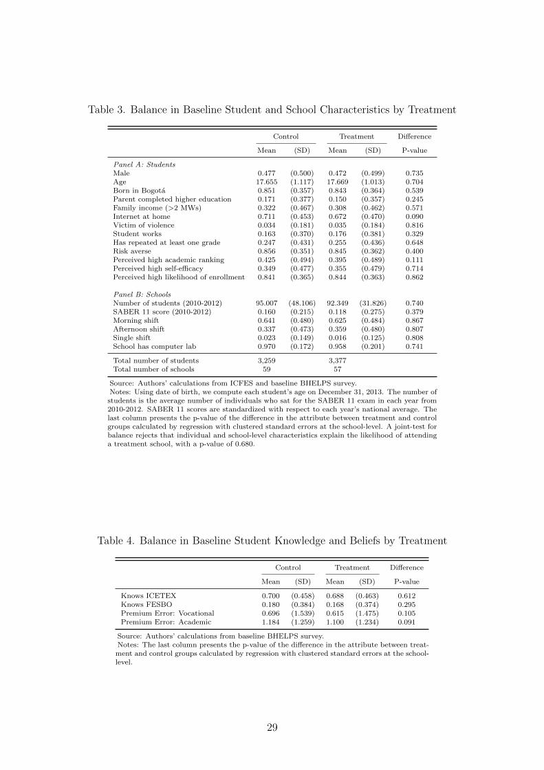
Table 3. Balance in Baseline Student and School Characteristics by Treatment

Control Treatment Difference

Mean (SD) Mean (SD) P-value

Panel A: StudentsMale 0.477 (0.500) 0.472 (0.499) 0.735Age 17.655 (1.117) 17.669 (1.013) 0.704Born in Bogota 0.851 (0.357) 0.843 (0.364) 0.539Parent completed higher education 0.171 (0.377) 0.150 (0.357) 0.245Family income (>2 MWs) 0.322 (0.467) 0.308 (0.462) 0.571Internet at home 0.711 (0.453) 0.672 (0.470) 0.090Victim of violence 0.034 (0.181) 0.035 (0.184) 0.816Student works 0.163 (0.370) 0.176 (0.381) 0.329Has repeated at least one grade 0.247 (0.431) 0.255 (0.436) 0.648Risk averse 0.856 (0.351) 0.845 (0.362) 0.400Perceived high academic ranking 0.425 (0.494) 0.395 (0.489) 0.111Perceived high self-efficacy 0.349 (0.477) 0.355 (0.479) 0.714Perceived high likelihood of enrollment 0.841 (0.365) 0.844 (0.363) 0.862

Panel B: SchoolsNumber of students (2010-2012) 95.007 (48.106) 92.349 (31.826) 0.740SABER 11 score (2010-2012) 0.160 (0.215) 0.118 (0.275) 0.379Morning shift 0.641 (0.480) 0.625 (0.484) 0.867Afternoon shift 0.337 (0.473) 0.359 (0.480) 0.807Single shift 0.023 (0.149) 0.016 (0.125) 0.808School has computer lab 0.970 (0.172) 0.958 (0.201) 0.741

Total number of students 3,259 3,377Total number of schools 59 57

Source: Authors’ calculations from ICFES and baseline BHELPS survey.Notes: Using date of birth, we compute each student’s age on December 31, 2013. The number ofstudents is the average number of individuals who sat for the SABER 11 exam in each year from2010-2012. SABER 11 scores are standardized with respect to each year’s national average. Thelast column presents the p-value of the difference in the attribute between treatment and controlgroups calculated by regression with clustered standard errors at the school-level. A joint-test forbalance rejects that individual and school-level characteristics explain the likelihood of attendinga treatment school, with a p-value of 0.680.

Table 4. Balance in Baseline Student Knowledge and Beliefs by Treatment

Control Treatment Difference

Mean (SD) Mean (SD) P-value

Knows ICETEX 0.700 (0.458) 0.688 (0.463) 0.612Knows FESBO 0.180 (0.384) 0.168 (0.374) 0.295Premium Error: Vocational 0.696 (1.539) 0.615 (1.475) 0.105Premium Error: Academic 1.184 (1.259) 1.100 (1.234) 0.091

Source: Authors’ calculations from baseline BHELPS survey.Notes: The last column presents the p-value of the difference in the attribute between treat-ment and control groups calculated by regression with clustered standard errors at the school-level.

29

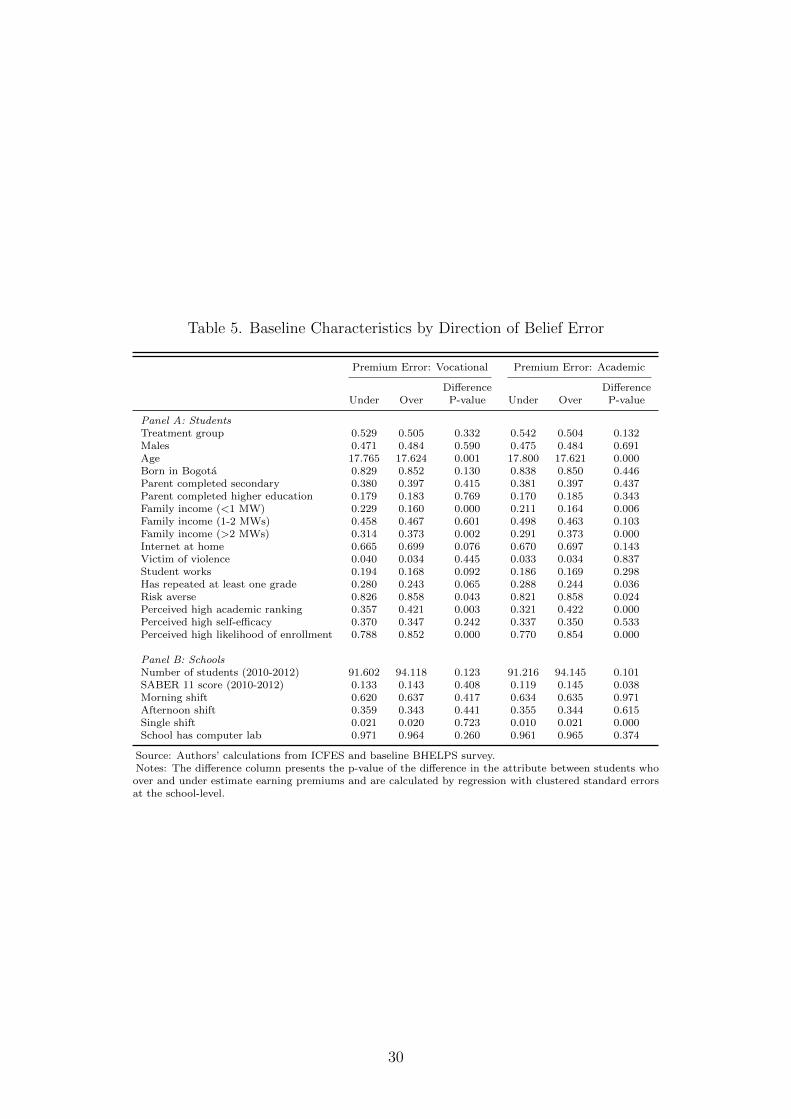
Table 5. Baseline Characteristics by Direction of Belief Error

Premium Error: Vocational Premium Error: Academic

Difference DifferenceUnder Over P-value Under Over P-value

Panel A: StudentsTreatment group 0.529 0.505 0.332 0.542 0.504 0.132Males 0.471 0.484 0.590 0.475 0.484 0.691Age 17.765 17.624 0.001 17.800 17.621 0.000Born in Bogota 0.829 0.852 0.130 0.838 0.850 0.446Parent completed secondary 0.380 0.397 0.415 0.381 0.397 0.437Parent completed higher education 0.179 0.183 0.769 0.170 0.185 0.343Family income (<1 MW) 0.229 0.160 0.000 0.211 0.164 0.006Family income (1-2 MWs) 0.458 0.467 0.601 0.498 0.463 0.103Family income (>2 MWs) 0.314 0.373 0.002 0.291 0.373 0.000Internet at home 0.665 0.699 0.076 0.670 0.697 0.143Victim of violence 0.040 0.034 0.445 0.033 0.034 0.837Student works 0.194 0.168 0.092 0.186 0.169 0.298Has repeated at least one grade 0.280 0.243 0.065 0.288 0.244 0.036Risk averse 0.826 0.858 0.043 0.821 0.858 0.024Perceived high academic ranking 0.357 0.421 0.003 0.321 0.422 0.000Perceived high self-efficacy 0.370 0.347 0.242 0.337 0.350 0.533Perceived high likelihood of enrollment 0.788 0.852 0.000 0.770 0.854 0.000

Panel B: SchoolsNumber of students (2010-2012) 91.602 94.118 0.123 91.216 94.145 0.101SABER 11 score (2010-2012) 0.133 0.143 0.408 0.119 0.145 0.038Morning shift 0.620 0.637 0.417 0.634 0.635 0.971Afternoon shift 0.359 0.343 0.441 0.355 0.344 0.615Single shift 0.021 0.020 0.723 0.010 0.021 0.000School has computer lab 0.971 0.964 0.260 0.961 0.965 0.374

Source: Authors’ calculations from ICFES and baseline BHELPS survey.Notes: The difference column presents the p-value of the difference in the attribute between students whoover and under estimate earning premiums and are calculated by regression with clustered standard errorsat the school-level.

30

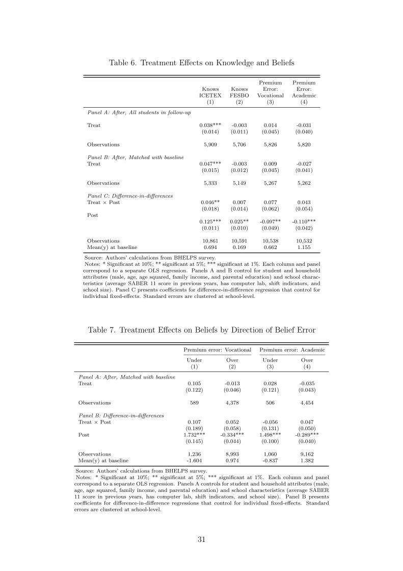
Table 6. Treatment Effects on Knowledge and Beliefs

Premium PremiumKnows Knows Error: Error:

ICETEX FESBO Vocational Academic(1) (2) (3) (4)

Panel A: After, All students in follow-up

Treat 0.038*** -0.003 0.014 -0.031(0.014) (0.011) (0.045) (0.040)

Observations 5,909 5,706 5,826 5,820

Panel B: After, Matched with baselineTreat 0.047*** -0.003 0.009 -0.027

(0.015) (0.012) (0.045) (0.041)

Observations 5,333 5,149 5,267 5,262

Panel C: Difference-in-differencesTreat × Post 0.046** 0.007 0.077 0.043

(0.018) (0.014) (0.062) (0.054)Post

0.125*** 0.025** -0.097** -0.110***(0.011) (0.010) (0.049) (0.042)

Observations 10,861 10,591 10,538 10,532Mean(y) at baseline 0.694 0.169 0.662 1.155

Source: Authors’ calculations from BHELPS survey.Notes: * Significant at 10%; ** significant at 5%; *** significant at 1%. Each column and panelcorrespond to a separate OLS regression. Panels A and B control for student and householdattributes (male, age, age squared, family income, and parental education) and school charac-teristics (average SABER 11 score in previous years, has computer lab, shift indicators, andschool size). Panel C presents coefficients for difference-in-difference regression that control forindividual fixed-effects. Standard errors are clustered at school-level.

Table 7. Treatment Effects on Beliefs by Direction of Belief Error

Premium error: Vocational Premium error: Academic

Under Over Under Over(1) (2) (3) (4)

Panel A: After, Matched with baselineTreat 0.105 -0.013 0.028 -0.035

(0.122) (0.046) (0.121) (0.043)

Observations 589 4,378 506 4,454

Panel B: Difference-in-differencesTreat × Post 0.107 0.052 -0.056 0.047

(0.189) (0.058) (0.131) (0.050)Post 1.732*** -0.334*** 1.498*** -0.289***

(0.145) (0.044) (0.100) (0.040)

Observations 1,236 8,993 1,060 9,162Mean(y) at baseline -1.604 0.974 -0.837 1.382

Source: Authors’ calculations from BHELPS survey.Notes: * Significant at 10%; ** significant at 5%; *** significant at 1%. Each column and panelcorrespond to a separate OLS regression. Panels A controls for student and household attributes (male,age, age squared, family income, and parental education) and school characteristics (average SABER11 score in previous years, has computer lab, shift indicators, and school size). Panel B presentscoefficients for difference-in-difference regressions that control for individual fixed-effects. Standarderrors are clustered at school-level.

31

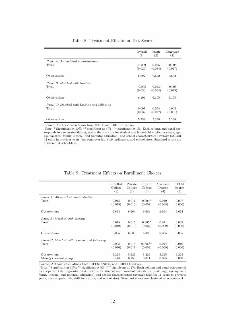
Table 8. Treatment Effects on Test Scores

Overall Math Language(1) (2) (3)

Panel A: All matched administrativeTreat -0.009 0.035 -0.008

(0.029) (0.034) (0.027)

Observations 6,692 6,692 6,692

Panel B: Matched with baselineTreat -0.005 0.043 -0.005

(0.030) (0.034) (0.029)

Observations 6,105 6,105 6,105

Panel C: Matched with baseline and follow-upTreat 0.007 0.054 0.003

(0.032) (0.037) (0.031)

Observations 5,238 5,238 5,238

Source: Authors’ calculations from ICFES and BHELPS survey.Note: * Significant at 10%; ** significant at 5%; *** significant at 1%. Each column and panel cor-responds to a separate OLS regression that controls for student and household attributes (male, age,age squared, family income, and parental education) and school characteristics (average SABER11 score in previous years, has computer lab, shift indicators, and school size). Standard errors areclustered at school-level.

Table 9. Treatment Effects on Enrollment Choices

Enrolled Private Top-10 Academic STEMCollege College College Degree Degree

(1) (2) (3) (4) (5)

Panel A: All matched administrativeTreat 0.015 0.011 0.004* 0.010 0.007

(0.019) (0.010) (0.002) (0.008) (0.006)

Observations 6,664 6,664 6,664 6,664 6,664

Panel B: Matched with baselineTreat 0.015 0.015 0.005* 0.011 0.009

(0.019) (0.010) (0.002) (0.009) (0.006)

Observations 6,085 6,085 6,085 6,085 6,085

Panel C: Matched with baseline and follow-upTreat 0.008 0.013 0.006** 0.014 0.010

(0.020) (0.011) (0.003) (0.009) (0.006)

Observations 5,225 5,225 5,225 5,225 5,225Mean(y) control group 0.444 0.153 0.011 0.095 0.050

Source: Authors’ calculations from ICFES, SNIES, and BHELPS survey.Note: * Significant at 10%; ** significant at 5%; *** significant at 1%. Each column and panel correspondsto a separate OLS regression that controls for student and household attributes (male, age, age squared,family income, and parental education) and school characteristics (average SABER 11 score in previousyears, has computer lab, shift indicators, and school size). Standard errors are clustered at school-level.

32

Table 10. Treatment Effects by Family Income and Gender (baseline matched to administrative data)

Knows Overall College Private Top-10 Academic STEMICETEX score Math Language Enrollment College College Degree Degree

(1) (2) (3) (4) (5) (6) (7) (8) (9)

Panel A: Average effectsTreat 0.038*** -0.005 0.043 -0.005 0.015 0.015 0.005* 0.011 0.009

(0.014) (0.030) (0.034) (0.029) (0.019) (0.010) (0.002) (0.009) (0.006)

Observations 5,909 6,105 6,105 6,105 6,085 6,085 6,085 6,085 6,085

Panel B: Treatment effects by family incomeLow Income (≤2MW) 0.054*** -0.038 0.020 -0.053 0.003 0.021** 0.001 0.008 0.008

(0.017) (0.036) (0.037) (0.035) (0.021) (0.009) (0.002) (0.008) (0.006)Middle Income (>2MW) 0.009 0.050 0.082* 0.071* 0.037 0.009 0.012** 0.018 0.011

(0.017) (0.043) (0.045) (0.042) (0.025) (0.019) (0.005) (0.017) (0.013)

P-value (Low=Middle) 0.017 0.088 0.178 0.013 0.176 0.530 0.050 0.612 0.814Observations 5,909 6,105 6,105 6,105 6,085 6,085 6,085 6,085 6,085

Panel C: Treatment effects by GenderFemale 0.022 -0.048 0.014 -0.051 -0.005 0.004 0.003 0.005 0.003

(0.018) (0.037) (0.041) (0.040) (0.024) (0.014) (0.003) (0.011) (0.007)Male 0.056*** 0.039 0.072* 0.043 0.037* 0.026** 0.007* 0.018 0.016

(0.018) (0.040) (0.042) (0.035) (0.021) (0.013) (0.004) (0.012) (0.010)

P-value (Female=Male) 0.120 0.071 0.235 0.056 0.114 0.226 0.401 0.404 0.272Observations 5,909 6,105 6,105 6,105 6,085 6,085 6,085 6,085 6,085

Source: Authors’ calculations from ICFES, SNIES, and BHELPS survey.Note: * Significant at 10%; ** significant at 5%; *** significant at 1%. Each column and panel corresponds to a separate OLS regression that controlsfor student and household attributes (male, age, age squared, family income, and parental education) and school characteristics (average SABER 11 scorein previous years, has computer lab, shift indicators, and school size). Standard errors are clustered at school-level.

33

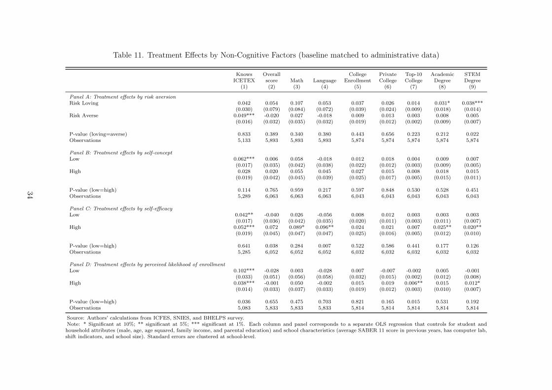
Table 11. Treatment Effects by Non-Cognitive Factors (baseline matched to administrative data)

Knows Overall College Private Top-10 Academic STEMICETEX score Math Language Enrollment College College Degree Degree

(1) (2) (3) (4) (5) (6) (7) (8) (9)

Panel A: Treatment effects by risk aversionRisk Loving 0.042 0.054 0.107 0.053 0.037 0.026 0.014 0.031* 0.038***

(0.030) (0.079) (0.084) (0.072) (0.039) (0.024) (0.009) (0.018) (0.014)Risk Averse 0.049*** -0.020 0.027 -0.018 0.009 0.013 0.003 0.008 0.005

(0.016) (0.032) (0.035) (0.032) (0.019) (0.012) (0.002) (0.009) (0.007)

P-value (loving=averse) 0.833 0.389 0.340 0.380 0.443 0.656 0.223 0.212 0.022Observations 5,133 5,893 5,893 5,893 5,874 5,874 5,874 5,874 5,874

Panel B: Treatment effects by self-conceptLow 0.062*** 0.006 0.058 -0.018 0.012 0.018 0.004 0.009 0.007

(0.017) (0.035) (0.042) (0.038) (0.022) (0.012) (0.003) (0.009) (0.005)High 0.028 0.020 0.055 0.045 0.027 0.015 0.008 0.018 0.015

(0.019) (0.042) (0.045) (0.039) (0.025) (0.017) (0.005) (0.015) (0.011)

P-value (low=high) 0.114 0.765 0.959 0.217 0.597 0.848 0.530 0.528 0.451Observations 5,289 6,063 6,063 6,063 6,043 6,043 6,043 6,043 6,043

Panel C: Treatment effects by self-efficacyLow 0.042** -0.040 0.026 -0.056 0.008 0.012 0.003 0.003 0.003

(0.017) (0.036) (0.042) (0.035) (0.020) (0.011) (0.003) (0.011) (0.007)High 0.052*** 0.072 0.089* 0.096** 0.024 0.021 0.007 0.025** 0.020**

(0.019) (0.045) (0.047) (0.047) (0.025) (0.016) (0.005) (0.012) (0.010)

P-value (low=high) 0.641 0.038 0.284 0.007 0.522 0.586 0.441 0.177 0.126Observations 5,285 6,052 6,052 6,052 6,032 6,032 6,032 6,032 6,032

Panel D: Treatment effects by perceived likelihood of enrollmentLow 0.102*** -0.028 0.003 -0.028 0.007 -0.007 -0.002 0.005 -0.001

(0.033) (0.051) (0.056) (0.058) (0.032) (0.015) (0.002) (0.012) (0.008)High 0.038*** -0.001 0.050 -0.002 0.015 0.019 0.006** 0.015 0.012*

(0.014) (0.033) (0.037) (0.033) (0.019) (0.012) (0.003) (0.010) (0.007)

P-value (low=high) 0.036 0.655 0.475 0.703 0.821 0.165 0.015 0.531 0.192Observations 5,083 5,833 5,833 5,833 5,814 5,814 5,814 5,814 5,814

Source: Authors’ calculations from ICFES, SNIES, and BHELPS survey.Note: * Significant at 10%; ** significant at 5%; *** significant at 1%. Each column and panel corresponds to a separate OLS regression that controls for student andhousehold attributes (male, age, age squared, family income, and parental education) and school characteristics (average SABER 11 score in previous years, has computer lab,shift indicators, and school size). Standard errors are clustered at school-level.

34

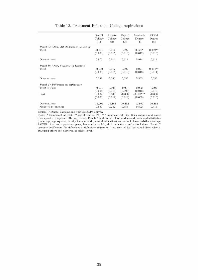
Table 12. Treatment Effects on College Aspirations

Enroll Private Top-10 Academic STEMCollege College College Degree Degree

(1) (2) (3) (4) (5)

Panel A: After, All students in follow-upTreat -0.001 0.014 0.022 0.021* 0.032**

(0.003) (0.015) (0.018) (0.012) (0.013)

Observations 5,976 5,914 5,914 5,914 5,914

Panel B: After, Students in baselineTreat -0.000 0.017 0.022 0.021 0.034**

(0.003) (0.015) (0.019) (0.013) (0.014)

Observations 5,389 5,333 5,333 5,333 5,333

Panel C: Difference-in-differencesTreat × Post -0.001 0.004 -0.007 0.002 0.007

(0.004) (0.016) (0.023) (0.013) (0.015)Post 0.004 0.009 -0.000 -0.028*** -0.006

(0.003) (0.012) (0.018) (0.009) (0.010)

Observations 11,006 10,862 10,862 10,862 10,862Mean(y) at baseline 0.983 0.232 0.457 0.892 0.417

Source: Authors’ calculations from BHELPS survey.Note: * Significant at 10%; ** significant at 5%; *** significant at 1%. Each column and panelcorrespond to a separate OLS regression. Panels A and B control for student and household attributes(male, age, age squared, family income, and parental education) and school characteristics (averageSABER 11 score in previous years, has computer lab, shift indicators, and school size). Panel Cpresents coefficients for difference-in-difference regression that control for individual fixed-effects.Standard errors are clustered at school-level.

35

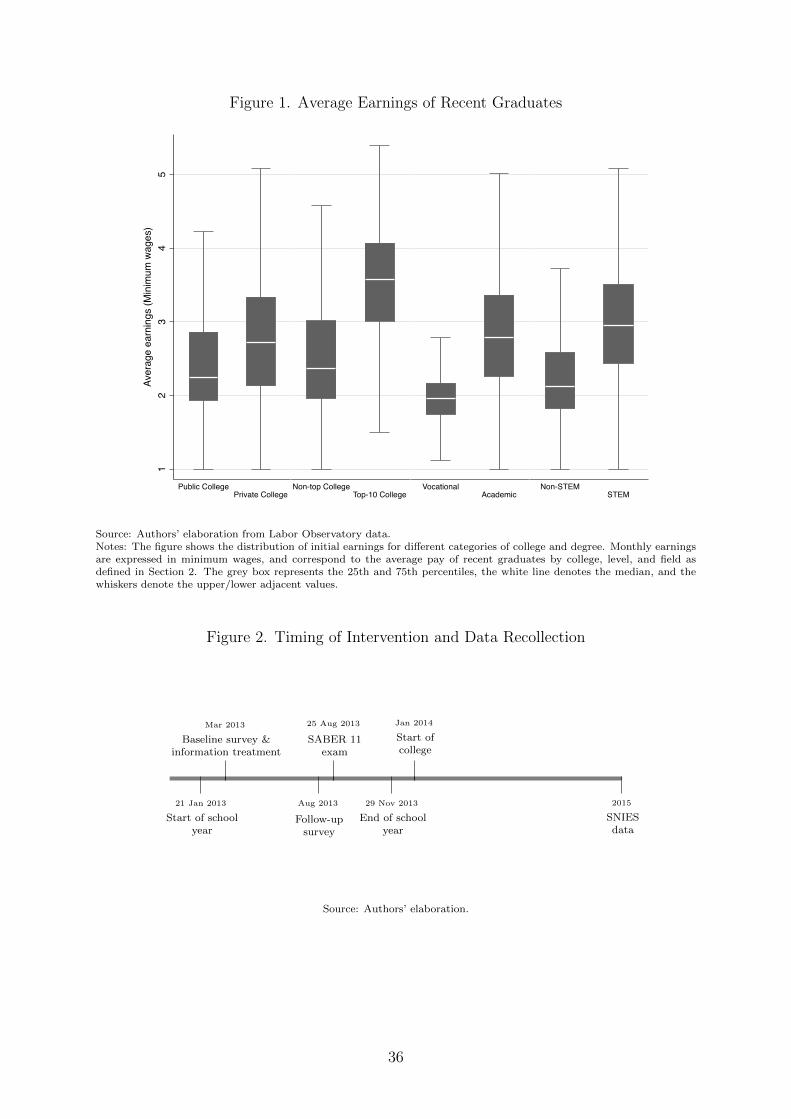
Figure 1. Average Earnings of Recent Graduates

12

34

5Av

erag

e ea

rnin

gs (M

inim

um w

ages

)

Public CollegePrivate College

Non-top CollegeTop-10 College

VocationalAcademic

Non-STEMSTEM

Source: Authors’ elaboration from Labor Observatory data.Notes: The figure shows the distribution of initial earnings for different categories of college and degree. Monthly earningsare expressed in minimum wages, and correspond to the average pay of recent graduates by college, level, and field asdefined in Section 2. The grey box represents the 25th and 75th percentiles, the white line denotes the median, and thewhiskers denote the upper/lower adjacent values.

Figure 2. Timing of Intervention and Data Recollection

21 Jan 2013

Start of schoolyear

Mar 2013

Baseline survey &information treatment

Aug 2013

Follow-upsurvey

25 Aug 2013

SABER 11exam

29 Nov 2013

End of schoolyear

Jan 2014

Start ofcollege

2015

SNIESdata

Source: Authors’ elaboration.

36

Figure 3. Geographic distribution of treatment and control schools

Source: Authors’ elaboration from Secretary of Education’s School Census and BHELPS.

37

Figure 4. Distribution of Earning Premium Beliefs at Baseline0.

00.

10.

20.

30.

40.

5Fr

actio

n

-1000 -500 0 500 1000% Error

Vocational (2-year)

0.0

0.1

0.2

0.3

0.4

0.5

Frac

tion

-1000 -500 0 500 1000% Error

Academic (4-year)

Source: Authors’ elaboration from BHELPS baseline sample.Notes: We calculate the error percentage as the difference between perceived and actual premiums divided by the ac-tual premium. Let πj denote the wage premium, with j = {actual,perceived}. Errors are calculated as (πperceived −πactual)/πactual.

Figure 5. Quantile treatment effects for SABER 11 test scores

-.10

.1.2

Qua

ntile

Tre

atm

ent E

ffect

0 .2 .4 .6 .8 1quantile

Mathematics

-.2-.1

0.1

.2Q

uant

ile T

reat

men

t Effe

ct

0 .2 .4 .6 .8 1quantile

Language

Source: Authors’ elaboration from ICFES and BHELPS survey.Notes: Estimates based on baseline matched to administrative data (N=6,105). 90% Confidence intervals in blackdashed/red dotted lines. OLS estimate in red dashed line. Standard errors clustered at the school-level.

38

Appendix

A.1 Student Handout

La relación entre estudios e ingresos

La educación superior es un factor determinante de la situación económica y por tanto la calidad de vida de las familias. En el siguiente gráfico se presentan los salarios promedio por nivel educativo en Bogotá.

Como se puede observar, mayor educación se traduce en salarios más altos. Sólo con terminar el Bachillerato se pasa de ganar 457.000 a 574.000 por mes. El salto es más evidente para aquellos con un título de nivel superior, ya que el salario promedio mensual crece a 1.482.000. Estas estadísticas presentan un mensaje claro: vale la pena estudiar.

¿Cómo puedo averiguar cuanto ganaría en la carrera que a mí me interesa?

Es probable que usted ya tenga una idea sobre las carreras que le interesarían y la institución donde quisiera realizar estos estudios. Si es así, ¿hay algu-na manera de saber cuánto puede esperar ganar en su situación específica?

Existen dos lugares donde pueden consultar el salario promedio de los graduados por institución y carreras. Estas son:

1. Calculadora de salarios promedios para graduados: www.finanzaspersonales.com.co

Esta página cuenta con una herramienta que le permite consultar el salario promedio por región, institución edu-cativa, programa de estudio y género de las personas que obtuvieron su título entre 2001-2011.

¿Cómo funciona?

• Acceda al enlace y busque la Calculadora de Salario por profesión para Graduados

457

0

400

600

800

1.000

1.200

1.400

1.600

No completaBachillerato

Bachillerato Superior oUniversitaria

(nivel de educación)

(miles de pesos)

574

1.482

200

• Escoja la región donde quiere realizar la búsqueda (por ejemplo, Bogotá)

• Seleccione la institución donde quiere realizar sus es-tudios y el programa que planea cursar

2. Observatorio laboral del Ministerio de Educación: www.graduadoscolombia.edu.co

Está página también provee información sobre los sala-rios promedios de personas con título de educación su-perior para toda Colombia. Además, le permite conocer las perspectivas laborales del programa de estudio de su interés.

¿Cómo funciona?

• Acceda al enlace y busque el botón rojo que dice Sis-tema de información del Observatorio Laboral.

• Si quiere conocer el número de graduados por car-rera, acceda a la pestaña que dice “Perfil nacional”. Después, escoja el departamento donde planea es-tudiar y obtendrá los datos de graduados por área de estudio.

Si desea saber cuántos individuos en su área de interés tienen un empleo formal (cotizando a la seguridad so-cial) y cuanto ganan en promedio vaya a ¨Vinculación laboral recién graduados¨. Aquí tiene la opción de bus-car por institución o por carrera.

Recuerde que estas páginas le permiten conocer el salario promedio de los profesionales graduados en su área de interés.

¿Qué necesito para entrar a la Universidad y la car-rera que me interesa?

1. Buenos resultados académicos: Uno de los crite-rios más importantes a la hora de buscar admisión a una institución de educación superior es el rendimiento académico. Muchas instituciones utilizan el puntaje del ICFES (SABER 11), y otras instituciones como la Uni-versidad Nacional que tienen su propio examen de ad-misión. En cualquier caso, estudiar aumenta las posibi-lidades de ser admitido y también las posibilidades de acceder a becas o financiación.

2. Financiación: Existen varias maneras de financiar la educación superior en Colombia. En general, tendrán preferencia los alumnos de escasos recursos y buen desempeño académico. Las siguientes son algunas op-ciones a tener en cuenta:

• Becas proveídas por cada institución por mérito aca-démico y/o escasos recursos. Consulte las políticas de beca ya que estas son diferentes para cada in-stitución.

• ICETEX: http://www.icetex.gov.co• Secretaría de Educación de Bogotá (Banco de cupos,

Fondo de Financiamiento de Educación Superior de Bogotá): http://www.sedbogota.edu.co/index.php/ed-ucacion-superior.html

Fuente: Encuesta de Hogares 2011, DANE

¡La educación superior paga!

39

Post-­‐secondary  education  pays!    

The  relation  between  studies  and  income    Higher  education   is  a  determining  factor  of  wages  and  the  quality   of   life   of   families.   The   following   figure   presents  average  wages  by  level  of  completed  education  in  Bogotá:    

 Clearly,   more   education   is   related   with   higher   wages.   By  only   finishing   high   school,   wages   move   from   457,000   to  574,000   pesos   each   month.   The   difference   is   even   more  marked  for  those  with  a  college  degree,  since  their  average  monthly   wage   increases   to   1,492,000.   These   statistics  present  a  clear  pattern:  studying  is  worth  it.    How   can   I   learn   about   how   much   people   earn   who  finished  the  degree  I’m  interested  in?    It  is  very  likely  that  you  already  have  a  good  idea  about  the  degrees   and   institutions   where   you   would   like   to   pursue  your   studies.   If   this   is   true,   is   there   a   way   to   know   how  much  I  could  expect  to  earn?    There  are  two  places  where  you  can  obtain  information  on  average   wages   for   graduates   by   institution   and   degree.  These  are:  1.   Average   wage   calculator   for   graduates:  

www.finanzaspersonales.com.co  This   website   counts   with   a   tool   that   allows   to   calculate  average  wages  by  region,  institution,  degree  and  gender  of  people  who  graduated  between  2001  and  2011.    How  does  it  work?  -­‐   Visit   the   website   and   search   for  Wage   calculator   by  

degree  for  Graduates.    

-­‐   Select  the  region  where  you  are  interested  in  searching  (e.g.  Bogotá)  

-­‐   Select   the   institution   and   the   degree   you   are   interested   in  evaluating  

2.   Labor   Observatory   of   the   Ministry   of   Education:  www.graduadoscolombia.edu.co  

This  website  also  provides   information  about  average  wages   for  the   whole   country.   Additionally,   you   can   learn   about   the   labor  prospects  for  your  degree  of  interest    How  does  it  work?  -­‐   Visit   the   website   and   click   on   the   red   button   reading  

Information  System  of  the  Labor  Observatory  -­‐   If   you   would   like   to   know   the   number   of   graduates   by  

degree,   click   on   the   “National   Profile”   tab.   Next,   select   the  department  where  you  plan   to   study  and  you  will   find  data  on  graduates  by  degree.  

 If   you   are   interested   in   the   number   of   individuals  who   pursued  your   degree   of   interest   who   have   a   formal   job   (paying   social  security)  and  how  much  they  earn  on  average,  select  “labor   link  of   recent   graduates”.   Here   you   have   the   option   to   search   by  institution  and  degree.    Remember  that  these  websites  allow  to  learn  about  the  average  wages  of  recent  graduates  for  your  degree  of  interest.    What  will   I   need   to  enroll   in   a  University   and   in  my  degree  of  interest?  

 1.   Good   academic   results:   One   of   the   main   criteria   for  

admissions   in   University   if   academic   performance.   Many  institutions   use   the   ICFES   (SABER   11)   score,   and   other  institutions   like   the  National  University   also   have   their   own  admissions   test.   Nevertheless,   studying   will   increase   the  probability  of  being  admitted  and  also  of  obtaining   financial  aid  or  financing.  

2.   Financing:  There  are  many  ways  to  finance  higher  education  in   Colombia.   In   general,   financing   institutions   have  preferences   for   students  of   low   income  and  good  academic  performance.   The   following  are   some  organizations   to   keep  in  mind:  

-­‐   Scholarships   provided   by   each   institution   according   to  academic   merit   of   financial   need.   Consult   the   scholarship  policies  for  each  institution  given  that  they  may  differ.  

-­‐   ICETEX:  http://www.icetex.gov.co  -­‐   Secretary   of   Education   in   Bogotá   (FDFESBO):  

http://www.sedbogota.edu.co/index.php/ed-­‐   ucacion-­‐superior.html  

 

40

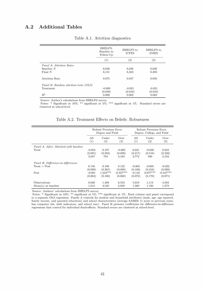
A.2 Additional Tables

Table A.1. Attrition diagnostics

BHELPS:Baseline toFollow-Up

BHELPS toICFES

BHELPS toSNIES

(1) (2) (3)

Panel A: Attrition RatesBaseline N 6,636 6,636 6,636Final N 6,141 6,323 6,303

Attrition Rate 0.075 0.047 0.050

Panel B: Random attrition tests (OLS)Treatment -0.009 -0.021 -0.021

(0.039) (0.016) (0.016)R2 0.000 0.002 0.002

Source: Author’s calculations from BHELPS survey.Notes: * Significant at 10%; ** significant at 5%; *** significant at 1%. Standard errors areclustered at school-level.

Table A.2. Treatment Effects on Beliefs: Robustness

Robust Premium Error Robust Premium ErrorDegree and Field Degree, College, and Field

All Under Over All Under Over(1) (2) (3) (1) (2) (3)

Panel A: After, Matched with baselineTreat -0.054 0.187 -0.089 0.021 -0.020 0.034

(0.091) (0.202) (0.090) (0.217) (0.516) (0.228)3,947 784 3,163 2,772 590 2,182

Panel B: Difference-in-differencesTreat × Post 0.146 0.106 0.122 -0.003 -0.005 -0.022

(0.099) (0.265) (0.098) (0.100) (0.316) (0.099)Post -0.091 1.243*** -0.337*** -0.116 0.977*** -0.347***

(0.064) (0.160) (0.068) (0.072) (0.170) (0.071)

Observations 8,020 1,468 6,552 5,618 1,114 4,504Mean(y) at baseline 1.613 -0.581 2.059 1.369 1.180 1.873

Source: Authors’ calculations from BHELPS survey.Notes: * Significant at 10%; ** significant at 5%; *** significant at 1%. Each column and panel correspondto a separate OLS regression. Panels A controls for student and household attributes (male, age, age squared,family income, and parental education) and school characteristics (average SABER 11 score in previous years,has computer lab, shift indicators, and school size). Panel B presents coefficients for difference-in-differenceregressions that control for individual fixed-effects. Standard errors are clustered at school-level.

41

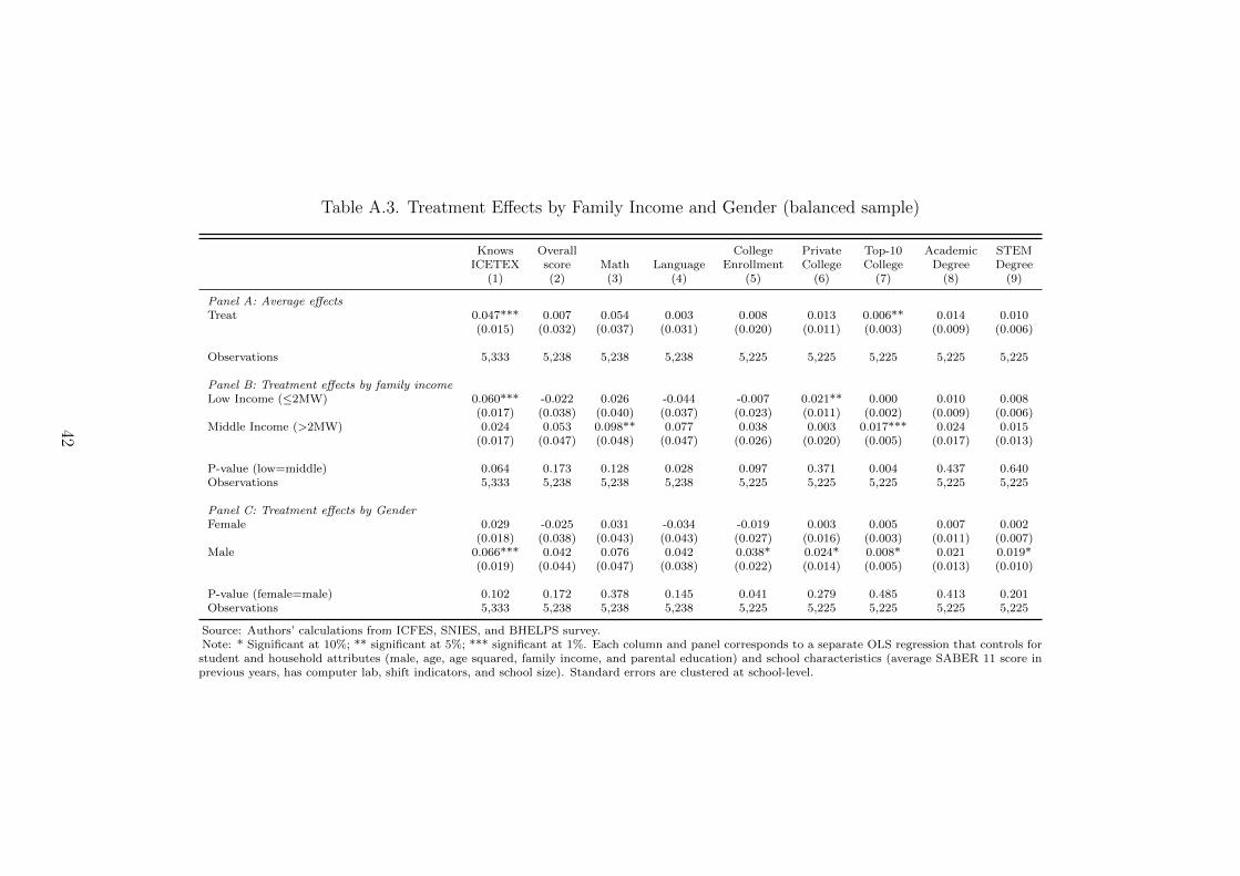
Table A.3. Treatment Effects by Family Income and Gender (balanced sample)

Knows Overall College Private Top-10 Academic STEMICETEX score Math Language Enrollment College College Degree Degree

(1) (2) (3) (4) (5) (6) (7) (8) (9)

Panel A: Average effectsTreat 0.047*** 0.007 0.054 0.003 0.008 0.013 0.006** 0.014 0.010

(0.015) (0.032) (0.037) (0.031) (0.020) (0.011) (0.003) (0.009) (0.006)

Observations 5,333 5,238 5,238 5,238 5,225 5,225 5,225 5,225 5,225

Panel B: Treatment effects by family incomeLow Income (≤2MW) 0.060*** -0.022 0.026 -0.044 -0.007 0.021** 0.000 0.010 0.008

(0.017) (0.038) (0.040) (0.037) (0.023) (0.011) (0.002) (0.009) (0.006)Middle Income (>2MW) 0.024 0.053 0.098** 0.077 0.038 0.003 0.017*** 0.024 0.015

(0.017) (0.047) (0.048) (0.047) (0.026) (0.020) (0.005) (0.017) (0.013)

P-value (low=middle) 0.064 0.173 0.128 0.028 0.097 0.371 0.004 0.437 0.640Observations 5,333 5,238 5,238 5,238 5,225 5,225 5,225 5,225 5,225

Panel C: Treatment effects by GenderFemale 0.029 -0.025 0.031 -0.034 -0.019 0.003 0.005 0.007 0.002

(0.018) (0.038) (0.043) (0.043) (0.027) (0.016) (0.003) (0.011) (0.007)Male 0.066*** 0.042 0.076 0.042 0.038* 0.024* 0.008* 0.021 0.019*

(0.019) (0.044) (0.047) (0.038) (0.022) (0.014) (0.005) (0.013) (0.010)

P-value (female=male) 0.102 0.172 0.378 0.145 0.041 0.279 0.485 0.413 0.201Observations 5,333 5,238 5,238 5,238 5,225 5,225 5,225 5,225 5,225

Source: Authors’ calculations from ICFES, SNIES, and BHELPS survey.Note: * Significant at 10%; ** significant at 5%; *** significant at 1%. Each column and panel corresponds to a separate OLS regression that controls forstudent and household attributes (male, age, age squared, family income, and parental education) and school characteristics (average SABER 11 score inprevious years, has computer lab, shift indicators, and school size). Standard errors are clustered at school-level.

42

Table A.4. Treatment Effects by Direction of Belief Error (baseline matched to administrative data)

Knows Overall College Private Top-10 Academic STEMICETEX score Math Language Enrollment College College Degree Degree

(1) (2) (3) (4) (5) (6) (7) (8) (9)

Panel A: Average effectsTreat 0.038*** -0.005 0.043 -0.005 0.015 0.015 0.005* 0.011 0.009

(0.014) (0.030) (0.034) (0.029) (0.019) (0.010) (0.002) (0.009) (0.006)

Observations 5,909 6,105 6,105 6,105 6,085 6,085 6,085 6,085 6,085

Panel B: Treatment effects by direction of belief errorUnderestimates 0.054 -0.001 0.127 -0.014 0.045 0.000 0.000 0.024 0.023

(0.034) (0.079) (0.079) (0.079) (0.033) (0.025) (0.005) (0.021) (0.014)Overestimates 0.049*** -0.012 0.028 -0.007 0.007 0.018 0.005* 0.008 0.008

(0.016) (0.031) (0.034) (0.031) (0.019) (0.011) (0.003) (0.009) (0.007)

P-value (over=under) 0.885 0.901 0.211 0.933 0.264 0.490 0.432 0.473 0.349Observations 5,909 6,105 6,105 6,105 6,085 6,085 6,085 6,085 6,085

Source: Authors’ calculations from ICFES, SNIES, and BHELPS survey.Note: * Significant at 10%; ** significant at 5%; *** significant at 1%. Each column and panel corresponds to a separate OLS regression that controls for studentand household attributes (male, age, age squared, family income, and parental education) and school characteristics (average SABER11 score in previous years,has computer lab, shift indicators, and school size). Standard errors are clustered at school-level.

43

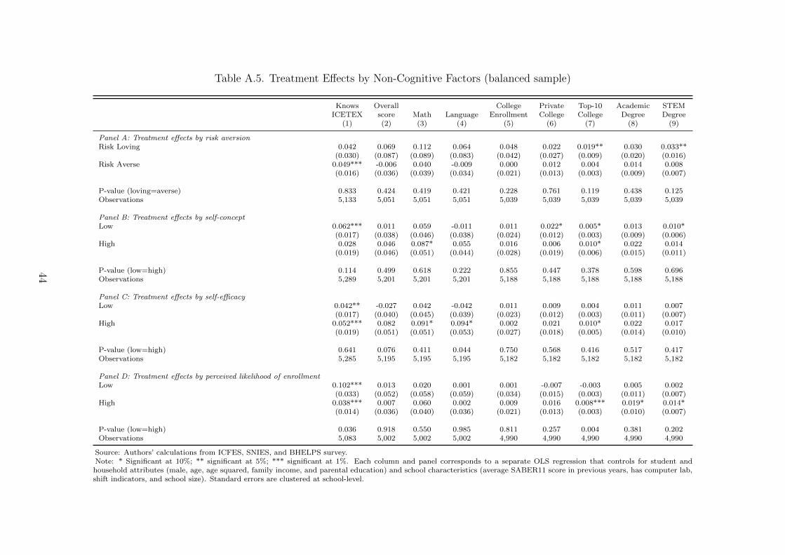
Table A.5. Treatment Effects by Non-Cognitive Factors (balanced sample)

Knows Overall College Private Top-10 Academic STEMICETEX score Math Language Enrollment College College Degree Degree

(1) (2) (3) (4) (5) (6) (7) (8) (9)

Panel A: Treatment effects by risk aversionRisk Loving 0.042 0.069 0.112 0.064 0.048 0.022 0.019** 0.030 0.033**

(0.030) (0.087) (0.089) (0.083) (0.042) (0.027) (0.009) (0.020) (0.016)Risk Averse 0.049*** -0.006 0.040 -0.009 0.000 0.012 0.004 0.014 0.008

(0.016) (0.036) (0.039) (0.034) (0.021) (0.013) (0.003) (0.009) (0.007)

P-value (loving=averse) 0.833 0.424 0.419 0.421 0.228 0.761 0.119 0.438 0.125Observations 5,133 5,051 5,051 5,051 5,039 5,039 5,039 5,039 5,039

Panel B: Treatment effects by self-conceptLow 0.062*** 0.011 0.059 -0.011 0.011 0.022* 0.005* 0.013 0.010*

(0.017) (0.038) (0.046) (0.038) (0.024) (0.012) (0.003) (0.009) (0.006)High 0.028 0.046 0.087* 0.055 0.016 0.006 0.010* 0.022 0.014

(0.019) (0.046) (0.051) (0.044) (0.028) (0.019) (0.006) (0.015) (0.011)

P-value (low=high) 0.114 0.499 0.618 0.222 0.855 0.447 0.378 0.598 0.696Observations 5,289 5,201 5,201 5,201 5,188 5,188 5,188 5,188 5,188

Panel C: Treatment effects by self-efficacyLow 0.042** -0.027 0.042 -0.042 0.011 0.009 0.004 0.011 0.007

(0.017) (0.040) (0.045) (0.039) (0.023) (0.012) (0.003) (0.011) (0.007)High 0.052*** 0.082 0.091* 0.094* 0.002 0.021 0.010* 0.022 0.017

(0.019) (0.051) (0.051) (0.053) (0.027) (0.018) (0.005) (0.014) (0.010)

P-value (low=high) 0.641 0.076 0.411 0.044 0.750 0.568 0.416 0.517 0.417Observations 5,285 5,195 5,195 5,195 5,182 5,182 5,182 5,182 5,182

Panel D: Treatment effects by perceived likelihood of enrollmentLow 0.102*** 0.013 0.020 0.001 0.001 -0.007 -0.003 0.005 0.002

(0.033) (0.052) (0.058) (0.059) (0.034) (0.015) (0.003) (0.011) (0.007)High 0.038*** 0.007 0.060 0.002 0.009 0.016 0.008*** 0.019* 0.014*

(0.014) (0.036) (0.040) (0.036) (0.021) (0.013) (0.003) (0.010) (0.007)

P-value (low=high) 0.036 0.918 0.550 0.985 0.811 0.257 0.004 0.381 0.202Observations 5,083 5,002 5,002 5,002 4,990 4,990 4,990 4,990 4,990

Source: Authors’ calculations from ICFES, SNIES, and BHELPS survey.Note: * Significant at 10%; ** significant at 5%; *** significant at 1%. Each column and panel corresponds to a separate OLS regression that controls for student andhousehold attributes (male, age, age squared, family income, and parental education) and school characteristics (average SABER11 score in previous years, has computer lab,shift indicators, and school size). Standard errors are clustered at school-level.

44

Table A.6. Baseline Balance in Student Aspirations

Control Treatment Difference

Mean (SD) Mean (SD) P-value

Enroll 0.988 (0.108) 0.988 (0.108) 1.000Public College 0.628 (0.484) 0.629 (0.483) 0.944Private College 0.220 (0.415) 0.234 (0.423) 0.403Top-10 College 0.451 (0.498) 0.470 (0.499) 0.442Academic degree (4-year) 0.886 (0.317) 0.897 (0.304) 0.359STEM degree 0.403 (0.491) 0.430 (0.495) 0.089

Source: Authors’ calculations from baseline BHELPS survey.Notes: The last column presents the p-value of the difference in the attribute between treat-ment and control groups calculated by regression with clustered standard errors at the school-level.

45