Information Externalities, Free Riding, and

Optimal Exploration in the UK Oil Industry

Charles Hodgson*

October 14, 2021

Abstract

Information spillovers between rms can reduce the incentive to invest in

R&D if property rights do not prevent rms from free riding on competitors'

innovations. Conversely, strong property rights over innovations can impede

cumulative research and lead to inecient duplication of eort. These eects are

particularly acute in natural resource exploration, where discoveries are spatially

correlated. I quantify these eects using data from oshore oil exploration

in the UK to estimate a dynamic structural model of the rm's exploration

problem. Firms face a trade-o between drilling now and delaying exploration

to learn from other rms' wells. Removing the incentive to free ride increases

industry surplus by 27% and allowing perfect information ow between rms

raises industry surplus by 5%. Counterfactual policy simulations highlight a

trade o in property rights design: stronger property rights over exploration

well data increase the rate of exploration, while weaker property rights increase

the eciency and speed of learning but reduce the rate of exploration. Spatial

clustering of each rm's drilling licenses both reduces the incentive to free ride

and increases the speed of learning.

Department of Economics, Yale Univeristy, 37 Hillhouse Avenue, New Haven, CT 06511 Email: charles.hodgson@yale.edu

*This research was supported by the Israel Dissertation Fellowship through a grant to the StanfordInstitute for Economic Policy Research. I am grateful to Liran Einav, Matthew Gentzkow, TimothyBresnahan, Paulo Somaini, Lanier Benkard, Brad Larsen, Nikhil Agarwal, Phil Haile, Steve Berry,Ariel Pakes, Ken Hendricks, Jackson Dorsey, Linda Welling, and participants at various seminarsand conferences for helpful comments on this project. Thanks also to Oonagh Werngren and JenBrzozowska for help with sourcing the data.

1

1 Introduction

The incentive for a rm to invest in research and development depends on the extent

to which it can benet from the investments of its competitors. If the knowledge

generated by R&D, such as new technologies, the results of experiments, or the dis-

covery of mineral deposits, is publicly observable, rms may have an incentive to free

ride on their competitors' innovations, for example by introducing similar products

or mining in locations near their rivals' discoveries. When each rm would rather

wait to observe the results of other rms' research than invest in R&D themselves,

the equilibrium rate of innovation can fall below the socially optimal level (Bolton

and Harris, 1999). On the other hand if information ow between rms is limited,

for example by property rights on existing innovations, the progress of research may

be slowed because of inecient duplication and the inability of researchers to build

on each other's discoveries (Williams, 2013).

Policy that denes property rights over innovations plays an important role in con-

trolling the eects of information externalities and balancing the trade o between

discouraging free riding and encouraging cumulative research. For example, broader

patents minimize the potential for free riding but increase the cost of research that

builds on existing patents, and may therefore direct research investment away from

socially ecient projects (Scotchmer, 1991).

In this paper, I quantify the eects of information externalities on R&D in the context

of oil exploration. Several features of this industry make it an ideal setting for studying

the general problem of information spillovers and the design of optimal property rights

regulation. When an oil rm drills an exploration well it generates knowledge about

the presence or absence of resources in a particular location. Exploration wells can

therefore be thought of as experiments with observable outcomes located at points in

geographic space. Since oil deposits are spatially correlated, the result of exploration

in one location generates information about the likelihood of nding oil in nearby,

unexplored locations. The spatial nature of research in this industry means that the

extent to which dierent experiments are more or less closely related is well dened.

Research is cumulative in the sense that the ndings from exploration wells direct the

location of future wells and the decision to develop elds and extract oil.

Since multiple rms operate in the same region, the results of rival rms' wells provide

2

information that can determine the path of a rm's exploration. If rms can see the

results of each other's exploration activity, then there is an incentive to free ride

and delay investment in exploration until another rm has made discoveries that can

direct subsequent drilling. However, if the results of exploration are condential then

rms are likely to engage in wasteful exploration of regions that are known by other

rms to be unproductive.1 I use data covering the history of oshore drilling in the

UK between 1964 and 1990 to quantify these ineciencies and the extent to which

they can be mitigated by counterfactual property rights policies. The magnitude of

these eects depends on the spatial correlation of well outcomes, the extent to which

rms can observe the results of each others' wells, and the spatial arrangement of

drilling licenses assigned to dierent rms.

I start by measuring the spatial correlation of well outcomes. I t a logistic Gaussian

process model to data on the locations and outcomes of all exploration wells drilled

before 1990. This model allows binary outcomes - wells are either successful or un-

successful - to be correlated across space. The estimated Gaussian process can be

used as a Bayesian prior that embeds spatial learning. When a successful or unsuc-

cessful well is drilled, the implied posterior beliefs about the probability of nding oil

are updated at all other locations, with the perceived probability at nearby locations

updating more than at distant locations. The updating rule corresponds to a geosta-

tistical technique for interpolating over space that is widely used in natural resource

exploration.

The estimated spatial correlation indicates that the results of exploration wells should

have a signicant eect on beliefs about the probability of well success at distances of

up to 50 km. To test whether rm behavior is consistent with this spatial correlation,

I regress rm drilling decisions on past well results. I nd that rms' probability

of exploration at a location is signicantly increasing in the number of successful

past wells and signicantly decreasing in the number of unsuccessful past wells. The

response declines in distance in line with the measured spatial correlation. Firms'

response to the results of their own past wells is 2 to 5 times as as large as their

1This trade-o between free riding and inecient exploration has been identied as important forpolicy making in the industry literature. For example, in their survey of UK oil and gas regulation,Rowland and Hann (1987, p. 13) note that if it is not possible to exclude other companies fromthe results of an exploration well... companies will wait for other companies' drilling results andexploration will be deferred, but if information is treated highly condentially... an unregulatedmarket would be likely to generate repetitious exploration activity.

3

response to other rms' wells, suggesting imperfect information ow between rms.

I also measure how exploration probability varies with the spatial distribution of

property rights. Drilling licenses are issued to rms on 22x18 km blocks. I nd

that the monthly probability of exploration on a block increases signicantly in the

share of nearby blocks licensed to the same rm. This eects are statistically and

economically signicant and consistent with the presence of a free riding incentive -

rms are less likely to explore where there is a greater potential to learn from other

rms' exploration.

Together, these descriptive ndings suggest that information spillovers over space and

between rms play an important role in rms' exploration decisions. To measure the

eect of these externalities on equilibrium exploration rates and industry surplus I

incorporate the model of spatial beliefs into a structural model of the rm's explo-

ration problem. Firms face a dynamic discrete choice problem in which, each period,

they can choose to drill exploration wells on the set of blocks over which they have

property rights. At the end of each period rms observe the results of their explo-

ration wells, observe the results of other rm's wells with some probability, α ∈ [0, 1],

and update their beliefs about the spatial distribution of oil. Firms face a trade o

between drilling now and delaying exploration to learn from the results of other rms'

wells that depends on the spatial arrangement of drilling licenses and the probability

of observing the results of other rms' wells.

The model's asymmetric information structure complicates the rm's problem. Firms

observe dierent sets of well outcomes, and in order to forecast other rms' drilling

behavior each rm needs to form beliefs about the outcomes of unobserved wells and

about other rms' beliefs. To make estimation of the model and computation of

equilibrium tractable, I adopt the simplifying assumption that, in equilibrium, each

rm has beliefs about the rate of exploration of blocks held by other rms that are

correct in expectation, conditional on the rm's current state. The application of this

equilibrium assumption to a dynamic game of asymmetric information is similar to

the experience based equilibrium approach of Fershtman and Pakes (2012).

The estimated value of the spillover parameter, α, indicates that rms observe the

results of other rms' wells with 71% probability. The presence of substantial but

imperfect information spillovers means that equilibrium exploration behavior could

be aected by both free riding - since rms observe each other's well results and have

4

an incentive to delay exploration - and inecient exploration - since spillovers are

imperfect, each rm has less information on which to base its drilling decisions than

the set of all rms combined.

I perform counterfactual simulations to quantify these two eects. First, I remove the

incentive for rms to free ride and simulate counterfactual exploration and develop-

ment behavior. I nd that exploration and development is brought forward in time by

about 1.5 years, increasing the number of exploration wells drilled between 1964 and

1990 by about 17.5%. Removing free riding increases the 1964 present discounted

value of 1964-1990 industry surplus by 27%. Next, I allow for perfect information

sharing between rms, holding rms' incentive to free ride xed at the baseline level.

The number of exploration wells increases by 3% and the eciency of exploration

increases substantially - since rms can perfectly observe each other's well results,

cumulative learning is faster. The number of exploration wells per block developed

falls and exploration wells are more concentrated on productive blocks. Industry

surplus is 5% higher than the baseline in this information sharing counterfactual.

I next ask to what extent these ineciencies could be mitigated through alternative

property rights. Under UK regulations, data from exploration wells is property of the

rm for ve years before being made public. Weakening property rights by shortening

the condentiality window will increase the ow of information between rms, and is

likely to increase the eciency of exploration but may also increase the incentive to

free ride. On the other hand, strengthening property rights by extending the conden-

tiality window will decrease the incentive to free ride but slow cumulative learning and

reduce the eciency of exploration. I simulate equilibrium behavior under dierent

condentiality window lengths and nd that industry surplus is increased under both

longer and shorter condentiality windows. The revenue-maximizing window length

appears to be between 0 and 5 years, with a window length of 2.5 years increasing

revenue by 23% over the baseline.

Finally, I show how the spatial distribution of property rights aects exploration in-

centives. When each rm's drilling licenses neighbor fewer other-rm licenses the

incentive for rms to delay exploration is reduced and the value to rms of the infor-

mation generated by their own wells is greater. I construct a counterfactual spatial

assignment of property rights that clusters each rm's licenses together, holding the

total number of blocks assigned to each rm xed. Under the clustered assignment

5

the number of exploration wells drilled increases by 8% and the revenue increases by

18%. I do not claim that this is the optimal arrangement of property rights, so these

gures represent a lower bound on the possible eect of spatial reorganization.

The results highlight the tension between discouraging free riding and encouraging

ecient cumulative research in the design of property rights over innovations. In this

setting, there are ranges of the policy space in which strengthening property rights

leads to a marginal improvement in surplus and ranges where weakening property

rights is optimal. This trade o applies in other settings, for example in dening the

breadth of patents, regulations about the release of data from clinical trials, and the

property rights conditions attached to public funding of research. The quantitative

results on the spatial assignment of licenses can be thought of as an example of decen-

tralized research where a principal (here, the government) assigns research projects to

independent agents (here, rms). The results suggest that there are signicant gains

from assignments of projects that minimize the potential for information spillovers

across agents. This nding could be applied to, for example, publicly funded research

eorts that coordinate the activity of many independent scientists.

This paper contributes to the large literature on rms' incentives to conduct R&D

(Arrow, 1971; Dasgupta and Stiglitz, 1980; Spence, 1984). In particular, I build

on recent papers that ask whether and to what extent intellectual property rights

hinder subsequent innovation (Murray and Stern, 2007; Williams, 2013; Murray et

al., 2016). I contribute to this literature by quantifying the trade o between this

eect on cumulative research and the free riding incentive that has been discussed

in the theory literature (Hendricks and Kovenock, 1989; Bolton and Farrell, 1990;

Bolton and Harris, 1999). This paper diers from much of the innovation literature by

using a structural model of the rm's sequential research (here, exploration) problem

to quantify the eects of information externalities and alternative property rights

policies.

The results in this paper also contribute to an existing empirical literature on the eect

of information externalities in oil exploration. Much of this literature has focused on

bidding incentives in license auctions using data from the Gulf of Mexico (Porter,

1995; Haile, Hendricks, and Porter 2010; Nguyen, 2021). Less attention has been

given to the post-licensing exploration incentives induced by dierent property rights

policies. Notable exceptions include Hendricks and Porter (1996), who show that the

6

probability of exploration on tracts in the Gulf of Mexico increases sharply when rms

drilling licenses are close to expiry, and Lin (2009) and Levitt (2016), who document

rms' drilling response to exploration on nearby tracts.

Existing papers on oil and gas exploration that estimate structural models of the rm's

exploration problem include Levitt (2009), Lin (2013), Agerton (2018), and Steck

(2018). The model I estimate in this paper diers from existing work by incorporating

both Bayesian learning with spatially correlated beliefs and information leakage across

rms. This allows me to simulate exploration paths under counterfactual policies

which change the dependence of each rm's beliefs on the results of other rms'

exploration wells, for example under dierent spatial assignments of blocks to rms.

Steck (2018) uses a closely related dynamic model of the rm's decision of when to

drill in the presence of social learning about the optimal inputs to hydraulic fracturing.

Steck's nding of a signicant free riding eect when there is uncertainty about the

optimal technology is complementary to the ndings of this paper, which measures

the free riding eect in the presence of uncertainty about the location of oil deposits.

Other related papers in the economics of oil and gas exploration include Kellogg

(2011), who provides evidence of learning about drilling technology, showing that

pairs of oil production companies and drilling contractors develop relationship-specic

knowledge, and Covert (2015), who investigates rm learning about the optimal

drilling technology at dierent locations in North Dakota's Bakken Shale. Covert's

methodology is particularly close to mine, as he also uses a Gaussian process to model

rms' beliefs about the eectiveness of dierent drilling technologies in dierent loca-

tions. The results I present in Section 4, which show that rms are more likely to drill

exploration wells in locations where the outcome is more uncertain, contrast with the

ndings of Covert (2015), who shows that oil rms do not actively experiment with

fracking technology when the optimal choice of inputs in uncertain.

Finally, the procedure used to estimate the structural model of the rm's exploration

problem builds on the literature on estimation of dynamic games using conditional

choice probability methods, following Hotz and Miller (1993), Hotz, Miller, Sanders,

and Smith (1994), Bajari, Benkard, and Levin (2007), and Fershtman and Pakes

(2012). In particular, I extend these methods to a setting with asymmetric infor-

mation in which the econometrician is uninformed about each agent's information

set. I propose a novel source of identication of conditional chose probabilities in the

7

presence of this latent state variable that is dierent from the panel variation used

by Kasahara and Shimotsu (2008)

The remainder of this paper proceeds as follows. Section 2 provides an overview of

the setting and a summary of the data. Section 3 presents a model of spatial be-

liefs about the location of oil deposits. Section 4 presents reduced form results that

provide evidence of spatial learning, information spillovers, and free riding. In Sec-

tion 5 I develop a dynamic structural model of optimal exploration with information

spillovers, and in Section 6 I discuss estimation of the model. Results and policy

counterfactuals are presented in Sections 7 and 8. Section 9 concludes.

2 UK Oil Exploration: Setting and Data

I use data covering the history of oil drilling in the UK Continental Shelf (UKCS)

from 1964 to 1990. Oil exploration and production on the UKCS is carried out by

private companies who hold drilling licenses issued by the government. The rst such

licenses were issued in 1964, and the rst successful (oil yielding) well was drilled in

1969. Discoveries of the large Forties and Brent oil elds followed in 1970 and 1971.

Drilling activity took o after the oil price shock of 1973, and by the 1980s the North

Sea was an important producer of oil and gas. I focus on the region of the UKCS

north of 55°N and east of 2°W , mapped in Figure 1, which is bordered on the north

and east by the Norwegian and Faroese economic zones. This region contains the

main oil producing areas of the North Sea and has few natural gas elds, which are

mostly south of 55°N .

2.1 Technology

Oshore oil production can be divided into two phases of investment and two distinct

technologies. First, oil reservoirs must be located through the drilling of exploration

wells. These wells are typically drilled from mobile rigs or drill ships and generate

information about the geology under the seabed at a particular point, including the

presence or absence of oil in that location. It is important to note that the results of a

single exploration well provide limited information about the size of an oil deposit, and

many exploration wells must be drilled to estimate the volume of a reservoir. When a

8

suciently large oil eld has been located, the eld is developed. This second phase of

investment involves the construction of a production platform, a large static facility

typically anchored to the sea bed by stilts or concrete columns with the capacity to

extract large volumes of oil.

I observe the coordinates and operating rm of every exploration well drilled and

development platform constructed from 1964 to 1990. The left panel of Figure 1

maps exploration wells in the relevant region. For each exploration well, I observe a

binary outcome - whether or not it was successful. In industry terms, a successful

exploration well is one that encounters an oil column, and an unsuccessful well is a

dry hole. In reality, although exploration wells yield more complex geological data,

the success rate of wells based on a binary wet/dry classication is an important

statistic in determining whether to develop, continue exploring, or abandon a region.

See for example Lerche and MacKay (1995) and Bickel and Smith (2006) who present

models of optimal sequential exploration decisions based on binary signals. I observe

each development platform's monthly oil and gas production in m3 up to the year

2000.

2.2 Regulation

The UKCS is divided into blocks measuring 12x10 nautical miles (approx. 22x18

km). These blocks are indicated by the grid squares on the maps in Figure 1. The

UK government holds licensing rounds at irregular intervals (once every 1 to 2 years),

during which licenses that grant drilling rights over blocks are issued to oil and gas

companies. Unlike in many countries, drilling rights are not allocated by auctions.

Instead, the government announces a set of blocks that are available, and rms submit

applications which consist of a list of blocks, a portfolio of research on the geology

and potential productivity of the areas requested, a proposed drilling program, and

evidence of technical and nancial capacity. Applications for each block are evaluated

by government geoscientists. Although a formal scoring rubric allocates points for a

large number of assessment criteria including nancial competency, track record, use

of new technology, and the extent and feasibility of the proposed drilling program, the

assessment process allows government scientists and evaluators to exercise discretion

in determining the allocation of blocks to rms. Although the evaluation criteria have

changed over time, the discretionary system itself has remained relatively unchanged

9

since 1964.2

License holders pay an annual per-block fee, and are subject to 12.5% royalty pay-

ments on the gross value of all oil extracted. Licenses have an initial period of 4 or 6

years during which rms are required to carry out a minimum work requirement. I

refer to the end of this period as the license's work date. Minimum work requirements

are typically light, even in highly active areas. During the 1970s 3 exploration wells

per... 7 blocks became the norm in the main contested areas (Kemp, 2012a p.

58). Licenses in less contested frontier areas often did not require any drilling, only

seismic analysis.

Figure 1: Wells and License Blocks

Notes: Grid squares are license blocks. The left panel plots the location of all exploration wellsdrilled from 1964 to 1990. The right panel records license holders for each block in January 1975.Note that if multiple rms hold licenses on separate sections of a block, only one of those rms(chosen at random) is represented on this map.

I observe the history of license allocations for all blocks. I perform all analysis on a

region corresponding to the northern North Sea basin which contains almost all of

the large oil deposits discovered on the UK continental shelf.3 In assigning blocks

2A few blocks were oered at auction in the early 1970s, but this experiment was determinedto be unsuccessful. According to a regulatory manager at the Oil and Gas Authority (OGA), theresult of the auctions was that the Treasury raised a lot of money but nobody drilled any wells.By contrast, the discretionary system has stood the test of time. The belief among UK regulatorsis that auctions divert money away from rms' drilling budgets.

3Specically, this region corresponds to the area north of 55N , east of 0W , and south-west of the

10

to rms I make two important simplifying assumptions. First, I focus only on the

operator rm for each block. Licenses are often issued to consortia of rms, each

of which hold some share of equity on the block. The operator, typically the largest

equity holder, is given responsibility for day to day operations and decision making.

Non-operator equity holders are typically smaller oil companies that do not operate

any blocks themselves, and are often banks or other nancial institutions. Major

oil companies do enter joint ventures, with one of the companies acting as operator,

but these are typically long lasting alliances rather than block by block decisions.4

In the main analysis below, I will be ignoring secondary equity holders and treating

the operating rm as the sole decision maker, with all secondary equity holders being

passive investors.5 Second, licenses are sometimes issued over parts of blocks, splitting

the original blocks into smaller areas that can be held by dierent rms. All of the

analysis below will take place at the block level. Therefore, if two rms have drilling

rights on the two halves of block j, I will record them both as having independent

drilling rights on block j. In practice, 88.2% of licensed block-months have only

one license holder. 11.5% of block-months have two license holders and a negligible

fraction have more than two. Subject to these simplications, the right panel of

Figure 1 maps the locations of licensed blocks operated by the 5 largest rms in

January 1975. There are 73 unique operators between 1964 and 1990, but 90% of

block-months are operated by one of the top 25 rms, and over 50% are operated by

one of the top 5. Appendix Figure A1 illustrates the distribution of licenses at the

block-month level across rms.6

UK economic zone's border. For some of the descriptive exercises I restrict the data to 1970-1980,since the location of early exploration before any oil discoveries is hard to rationalize.

4For example, 97% of blocks operated by Shell between 1964 and 1990 were actually licensed toShell and Esso in a 50-50 split. Esso was at some point the operator of 16 unique blocks, comparedto more than 740 blocks that were joint ventures with Shell. Only 8.6% of block-months operatedby one of the top 5 rms (who together operate more than 50% of all block-months) have anothertop 5 rms as a secondary equity holder. This falls to 2.8% among the top 4 rms.

5Appendix Table A4 presents regressions of drilling probability on the distribution of surroundinglicenses that suggest this is a reasonable assumption. The number of nearby licenses operated bythe same rm as block j has a consistent, statistically signicant positive eect on the probabilityof exploration on block j. The number of nearby licenses with the same secondary equity holdersas block j, on which the operator of block j is a secondary equity holder, and on which one of thesecondary equity holders on block j is the operator, all have no statistically signicant eect ondrilling probability.

6One additional complication is the case of an oil reservoir which crosses multiple blocks operatedby dierent rms. In these cases the oil reservoir is unitized by regulation, and revenue is splitproportionally between operators of the blocks. This provision removes the common pool incentivediscussed by Lin (2013) and the incentive to develop an overlapping reservoir before a neighboring

11

A nal set of regulations dene property rights over the information generated by

wells. The production of development platforms is reported to the government and

published on a monthly basis. Data from exploration wells, including whether or not

the well was successful, is property of the rm for the rst ve years after a well

is drilled. After this condentiality period, well data is reported to the government

and made publicly available. In reality there is likely to be information ow between

rms during this condentiality period for a number of reasons: rms can exchange

or sell well data, information can leak through shared employees, contractors, or

investors, and the activities associated with a successful exploration well might be

visibly dierent than the activities associated with an unsuccessful exploration well.

The extent to which information ows between rms during this condentiality period

is an object of interest in the empirical analysis that follows.

2.3 Data

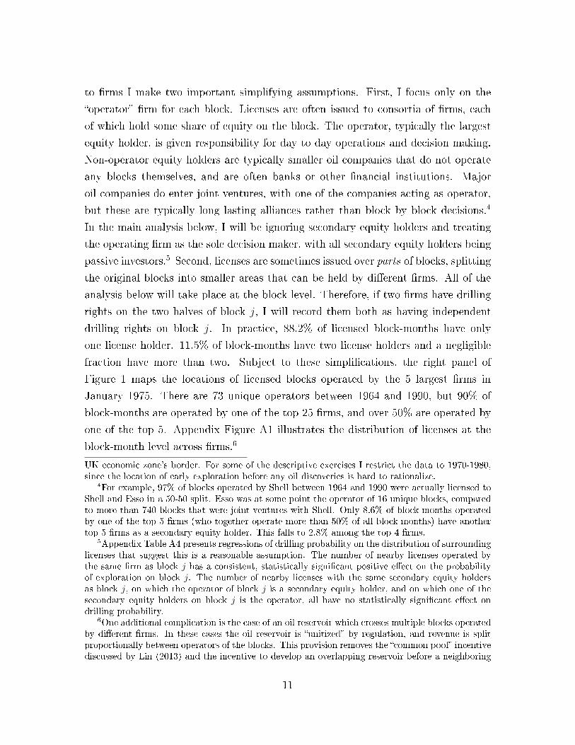
Table 1 contains summary statistics describing the data. Observations are at the

rm-block level. That is, if a particular block is licensed multiple times to dierent

rms, it appears in Table 1 as many times as it is licensed. There are a total of 628

blocks ever licensed and 1470 rm-block pairs between 1964 and 1990. I focus on two

actions - the drilling of exploration wells and the development of blocks. I consider

the development of a block as a one o decision to invest in a development platform.

I record a block as being developed on the drill date of the rst development well.

In reality, this would come several months after construction of the development

platform begins. I consider development to be a terminal action. Once a block is

developed, I drop it from the data.

The second column of Table 1 records statistics on the set of rm-blocks that are ever

explored - that is, those rm-blocks where at least one exploration well was drilled -

and the third column records statistics for those rm-blocks that are ever developed.

49% of rm-blocks are ever explored, and among these, 22% are developed. Note

that the information generated by a single well is insucient to establish the size

of an oil reservoir, and rms must drill many exploration wells on a block before

making the decision to develop. On average, over 10 exploration wells are drilled

rival.

12

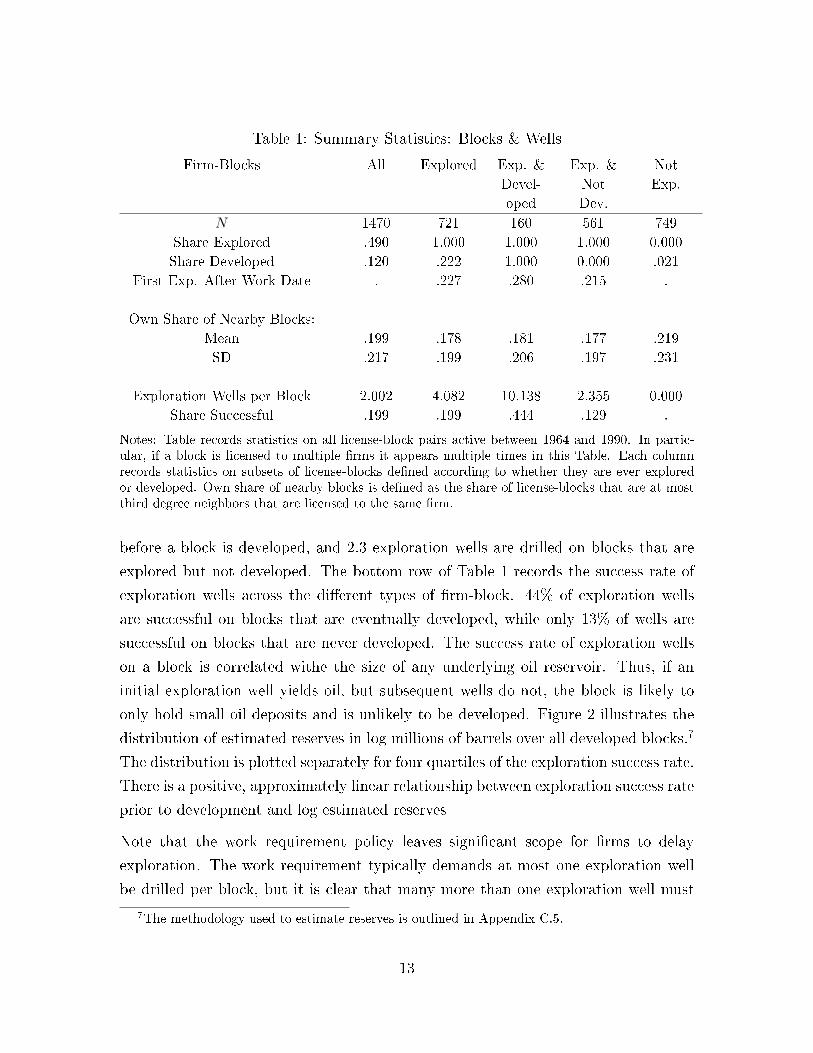
Table 1: Summary Statistics: Blocks & Wells

Firm-Blocks All Explored Exp. &

Devel-

oped

Exp. &

Not

Dev.

Not

Exp.

N 1470 721 160 561 749

Share Explored .490 1.000 1.000 1.000 0.000

Share Developed .120 .222 1.000 0.000 .021

First Exp. After Work Date . .227 .280 .215 .

Own Share of Nearby Blocks:

Mean .199 .178 .181 .177 .219

SD .217 .199 .206 .197 .231

Exploration Wells per Block 2.002 4.082 10.138 2.355 0.000

Share Successful .199 .199 .444 .129 .

Notes: Table records statistics on all license-block pairs active between 1964 and 1990. In partic-ular, if a block is licensed to multiple rms it appears multiple times in this Table. Each columnrecords statistics on subsets of license-blocks dened according to whether they are ever exploredor developed. Own share of nearby blocks is dened as the share of license-blocks that are at mostthird degree neighbors that are licensed to the same rm.

before a block is developed, and 2.3 exploration wells are drilled on blocks that are

explored but not developed. The bottom row of Table 1 records the success rate of

exploration wells across the dierent types of rm-block. 44% of exploration wells

are successful on blocks that are eventually developed, while only 13% of wells are

successful on blocks that are never developed. The success rate of exploration wells

on a block is correlated withe the size of any underlying oil reservoir. Thus, if an

initial exploration well yields oil, but subsequent wells do not, the block is likely to

only hold small oil deposits and is unlikely to be developed. Figure 2 illustrates the

distribution of estimated reserves in log millions of barrels over all developed blocks.7

The distribution is plotted separately for four quartiles of the exploration success rate.

There is a positive, approximately linear relationship between exploration success rate

prior to development and log estimated reserves

Note that the work requirement policy leaves signicant scope for rms to delay

exploration. The work requirement typically demands at most one exploration well

be drilled per block, but it is clear that many more than one exploration well must

7The methodology used to estimate reserves is outlined in Appendix C.5.

13

Figure 2: Estimated Reserves

02

46

8Log E

stim

ate

d R

eserv

es

.09 < SR < .27 .27 < SR < .38 .39 < SR < .54 .55 < SR < .71

Quartile of Exploration Success Rateexcludes outside values

Notes: Figure records the distribution of estimated oil reserve volume, measured in log millions ofbarrels, across all developed blocks in the relevant area. The box plot markers record the loweradjacent value, 25th percentile, median, 75th percentile, and upper adjacent value. The distributionis plotted separately for four subsets of blocks dened by the quartiles of the pre-developmentexploration well success rate. A regression of log estimated reserves on success rate has a slopecoecient of 5.990 with a standard error of 0.964.

be drilled before a block is developed. While the work requirement policy is therefore

likely to hasten the drilling of the rst exploration well on a block, there are no

requirements on the speed with which the subsequent program of exploration must

take place. The fourth row of Table 1 indicates that almost a quarter of blocks that

are ever explored are rst explored after the work requirement date. These ndings

corroborate claims from industry literature that indicate the terms of drilling licenses

issued in the UK are considerably more generous than those issued, for example, in

the Gulf of Mexico, and provide considerable room for rms to stockpile unexplored

and undeveloped acreage for many years (Gordon, 2015).

3 A Model of Spatially Correlated Beliefs

The eect of information externalities on rms' exploration decisions depends on the

spatial arrangement of licenses, the extent to which rms can observe the results of

14

each other's wells, and on the correlation of exploration results at dierent locations.

In Appendix A I show that in a simple two rm, two block model, spatial correlation in

well outcomes reduces the equilibrium rate of exploration below the social optimum.

The magnitude of this free riding eect is determined by the extent to which well

results are correlated over space. In particular, the more correlated are outcomes on

neighboring blocks, the lower the equilibrium rate of exploration.

In this section, I measure this spatial correlation by estimating a statistical model of

the distribution of oil that allows the results of exploration wells at dierent locations

to be correlated. By tting the model to data on the outcomes of all exploration

wells drilled between 1964 and 1990, I obtain an estimate of the extent to which this

covariance of well outcomes declines with distance. I interpret the estimated model

as describing the true spatial correlation of oil deposits determined by underlying

geology.

I then show how this statistical model can be used as a Bayesian prior about the

distribution of oil. If rms know the true parameter values, then the estimated model

implies a Bayesian updating rule for rms with rational beliefs. In particular, rms'

posterior beliefs about the probability of exploration well success at a given location

are a function of past well outcomes at nearby locations. The true correlation of well

outcomes informs the extent to which rms should make inferences over space when

updating their beliefs after observing well outcomes. This model of spatial learning

allows me to compute rms' posterior beliefs about the location of oil deposits after

observing dierent sets of wells.

3.1 Statistical Model of the Distribution of Oil

I start by describing a statistical model of the distribution of oil over space. I model

the probability that an exploration well at a particular location is successful as a

continuous function over space drawn from a Gaussian process. This model assumes

that the location of oil is distributed randomly over space but allows spatial correlation

- the outcomes of exploration wells close to each other are highly correlated and the

degree of correlation declines with distance. A draw from this process is a continuous

function that, depending on the parameters of the process, can have many local

maxima corresponding to separate clusters of oil elds (see Appendix Figure A2 for a

15

one dimensional example). As I discuss further below, Gaussian processes are widely

used in natural resource exploration to model the spatial distribution of geological

features (see for example Hohn, 1999).

Formally, let ρ(X) : X → [0, 1] be a function that denes the probability of explo-

ration well success at locations X ∈X. I model ρ(X) as being drawn from a logistic

Gaussian process G(ρ) over the space X.8 In particular, for any location X,

ρ(X) ≡ ρ(λ(X)) =1

1 + exp(−λ(X)), (1)

where λ(X) is a continuous function from X to R. Equation 1 is a logistic function

that squashes λ(X) so that ρ(X) ∈ [0, 1].

The function λ(X) is drawn from a Gaussian process with mean function µ(X) and

covariance function κ(X,X ′). This means that for any nite collection of K locations

1, ..., K, the vector (λ(X1), ..., λ(XK)) is a multivariate normal random variable

with mean (µ(X1), ..., µ(XK)) and a covariance matrix with (j, k) element κ(Xj, Xk).

The prior mean function µ : X → R is assumed to be smooth and the covariance

function κ : X ×X → R must be such that the resulting covariance matrix for any

K locations is symmetric and positive semi-denite. One covariance function that

satises these assumptions is the square exponential covariance function (Rasmussen

and Williams, 2006) given by

κ(X,X ′) = ω2exp

(− |X −X ′|2

2`2

). (2)

The parameter ω controls the variance of the process. In particular, for any X,

the marginal distribution of λ(X) is given by λ(X) ∼ N(µ(X), ω). The parameter

` controls the covariance between λ(X) and λ(X ′) for X 6= X ′. Notice that as

the distance |X −X ′| between two locations increases, the covariance falls at a rate

proportional to `. As |X −X ′| goes to 0, the correlation of λ(X) and λ(X ′) goes to

1, so draws from this process are continuous functions.

8If well success rates were independent across locations j, a natural model would draw ρj ∈ [0, 1]from a beta distribution. However, it is likely that well outcomes are correlated across space. Indeed,the results presented below in Figure 5 indicate that rms' exploration decisions on block j respondto the results of exploration wells on nearby blocks. There is no natural multivariate analogue ofthe beta distribution that allows me to specify a covariance between ρj and ρk for j 6= k.

16

I estimate the parameters, (µ(X), ω, `), of the Gaussian process model using data on

the binary outcomes of all well exploration wells drilled between 1964 and 1990. Let

s = (s1, s2, ..., sW ) be a vector of lengthW whereW is the total number of exploration

wells drilled by all rms and sw = 1 if well s was successful, and otherwise sw = 0.

Let X = (X1, ..., XW ) be a matrix recording the block centroid coordinates of each

well. Then the likelihood of well outcomes s conditional on well locations X is given

by:9

L(s|X,µ, ω, `) =

∫ ( W∏w=1

ρ(Xw)1(sw=1)(1− ρ(Xw))1(sw=0)

)dG(ρ;µ, ω, `) (3)

The integrand is the product of Bernoulli likelihoods for each well for a particular

draw of ρ, which encodes success probabilities at every location Xw. The integral

is over draws of ρ with respect to the distribution G(ρ), which is a function of the

parameters. Note that I assume a at mean function, µ(X) = µ(X ′) = µ.

Table 2 records maximum likelihood estimates. The rst column records the es-

timated values of the three parameters of the Gaussian process, while the second

column records implied statistics of the distribution of ρ(X) at the estimated param-

eters - the expected success probability, the standard deviation of success probability,

and the correlation of success probability between two locations one block (18 km)

away from each other. The parameters are identied by the empirical analogues of

these statistics in the well outcome data. Most importantly, the estimated parameter

` captures the true spatial correlation of exploration well outcomes.

3.2 Interpretation as a Bayesian Prior

The estimated parameters, (µ, ω, `), can be thought of as describing primitive geo-

logical characteristics that determine the distribution of oil deposits over space. If

9The consistency of maximum likelihood estimates of Gaussian Process parameters is not obvious,and the subject of a signicant literature in spatial statistics (see Mardia and Marshall, 1984, andCressie, 1991). In general, estimates generated using likelihoods of the form 3 are consistent underincreasing-domain asymptotics. That is, xing any set of locations X, every X ∈X is explored fora suciently large sample. This asymptotic framework is consistent with the assumption that thedata is generated by model of license issuing and exploration outlined in Section 5. Small samplebias due to the selection of explored blocks remains a concern, but such selection should be limitedsince 91% of licensed blocks have been explored at least once by 1990.

17

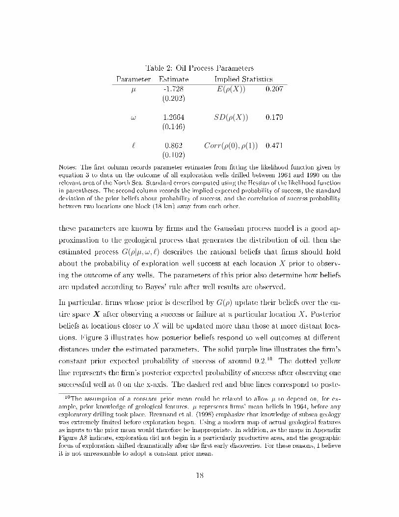
Table 2: Oil Process Parameters

Parameter Estimate Implied Statisticsµ -1.728 E(ρ(X)) 0.207

(0.202)

ω 1.2664 SD(ρ(X)) 0.179(0.146)

` 0.862 Corr(ρ(0), ρ(1)) 0.471(0.102)

Notes: The rst column records parameter estimates from tting the likelihood function given byequation 3 to data on the outcome of all exploration wells drilled between 1964 and 1990 on therelevant area of the North Sea. Standard errors computed using the Hessian of the likelihood functionin parentheses. The second column records the implied expected probability of success, the standarddeviation of the prior beliefs about probability of success, and the correlation of success probabilitybetween two locations one block (18 km) away from each other.

these parameters are known by rms and the Gaussian process model is a good ap-

proximation to the geological process that generates the distribution of oil, then the

estimated process G(ρ|µ, ω, `) describes the rational beliefs that rms should hold

about the probability of exploration well success at each location X prior to observ-

ing the outcome of any wells. The parameters of this prior also determine how beliefs

are updated according to Bayes' rule after well results are observed.

In particular, rms whose prior is described by G(ρ) update their beliefs over the en-

tire space X after observing a success or failure at a particular location X. Posterior

beliefs at locations closer to X will be updated more than those at more distant loca-

tions. Figure 3 illustrates how posterior beliefs respond to well outcomes at dierent

distances under the estimated parameters. The solid purple line illustrates the rm's

constant prior expected probability of success of around 0.2.10 The dotted yellow

line represents the rm's posterior expected probability of success after observing one

successful well at 0 on the x-axis. The dashed red and blue lines correspond to poste-

10The assumption of a constant prior mean could be relaxed to allow µ to depend on, for ex-ample, prior knowledge of geological features. µ represents rms' mean beliefs in 1964, before anyexploratory drilling took place. Brennand et al. (1998) emphasize that knowledge of subsea geologywas extremely limited before exploration began. Using a modern map of actual geological featuresas inputs to the prior mean would therefore be inappropriate. In addition, as the maps in AppendixFigure A8 indicate, exploration did not begin in a particularly productive area, and the geographicfocus of exploration shifted dramatically after the rst early discoveries. For these reasons, I believeit is not unreasonable to adopt a constant prior mean.

18

riors after observing two and three successful wells at the same location. Notice that

the expected probability of success increases most at the well location, and decreases

smoothly at more distant locations.

The true spatial correlation of well outcomes, captured by the parameter `, determines

the rate at which belief updating declines with distance. In particular, the estimated

value of ` implies that rms should update their beliefs about the probability of success

in response to well outcomes on neighboring blocks and those two blocks away, but

not in response to well outcomes three or more blocks away. At these distances, the

correlation in well outcomes dies out and thus so does the implied response of beliefs

to well outcomes.11

Figure 3: Response of Beliefs to Well Outcomes

0 0.5 1 1.5 2 2.5 3 3.5 4

Distance from Well (Blocks)

0.1

0.15

0.2

0.25

0.3

0.35

0.4

0.45

0.5

0.55

0.6

Expecte

d P

robabili

ty o

f S

uccess

Post 3 Wells

Post 2 Wells

Post 1 Well

Prior

0 10 20 30 40 50 60 70

Distance from Well (Km)

Notes: Figure depicts prior and posterior expected value of ρ(X) in a one dimensional space forposteriors computed after observing one, two, and three successful wells at X = 0. The parameters(µ, ω, `) of the logistic Gaussian process prior are set to the estimated values from Table 2.

Formally, let w ∈ W index wells, let s(w) ∈ 0, 1 be the outcome of well w, and let

Xw denote the location of well w. If prior beliefs are given by the logistic Gaussian

11In Appendix Figure A3 I illustrate belief updating under dierent values of ` in a numericalexample.

19

Process G(ρ) then the posterior beliefs G′(ρ) after observing (s(w), Xw)w∈W are

given by

G′(ρ) = B(G(ρ), (s(w), Xw)w∈W ), (4)

where B(·) is a Bayesian updating operator. Since the signals that rms receive are

binary, there is no analytical expression for the posterior beliefs given the Gaussian

prior and the observed signals. In particular, G′(ρ) is non-Gaussian. I compute

posterior distributions using the Laplace approximation technique of Rasmussen and

Williams (2006) which provides a Gaussian approximation to the non-Gaussian pos-

terior G′(ρ). I discuss the procedure used to compute B(·) in more detail in Appendix

B. Using the Bayesian updating rule it is possible to generate posterior beliefs for any

set of observed well realizations. Appendix Figure A4 is a map of posterior beliefs

for a rm that observed the outcome of all exploration wells drilled from 1964-1990,

illustrating regions with dierent posteiror expected probability of success and un-

certainty. In general, the standard deviation of posterior beliefs is lower in regions

where more exploration wells have been drilled.

The Gaussian process model is a parsimonious approximation to more complex infer-

ences about nearby geology made by geologists based on exploration well results. The

method of spatial interpolation between observed wells that is achieved by computing

the Gaussian Process posterior is known in the geostatistics literature as Kriging (see

for example standard geostatistics textbooks such as Hohn, 1999). Kriging is a widely

applied statistical technique for making predictions about the distribution of geolog-

ical features, including oil deposits, over space. Standard Kriging of a continuous

variable corresponds exactly to Bayesian updating of a Gaussian process with contin-

uous, normally distributed signals. The model of beliefs employed here corresponds

to trans-Gaussian Kriging, so called because of the use of a transformed Gaussian

distribution (Diggle, Tawn, and Moyeed, 1998). Whether or not we think these beliefs

are a correct representation of how oil deposits are distributed, the model of learning

described above is representative of how geologists (and presumably oil companies)

think.

20

3.3 Beliefs and Development Payos

In what follows, I adopt the additional simplifying assumption that rms have beliefs

about the probability of success at the block level. In particular, let ρj = ρ(Xj) where

Xj are the coordinates of the centroid of block j ∈ 1, ..., J. When an exploration

well is drilled anywhere on block j, rms update their beliefs as if the success of

that well is drawn with probability ρj. One way to rationalize this assumption is

to assume that the locations of exploration wells within blocks are drawn uniformly

at random. The probability of success, ρj, then has a natural interpretation as the

share of block j that contains oil, and the observed success rate is an estimate of this

probability which becomes more precise as the number of wells on the block increases.

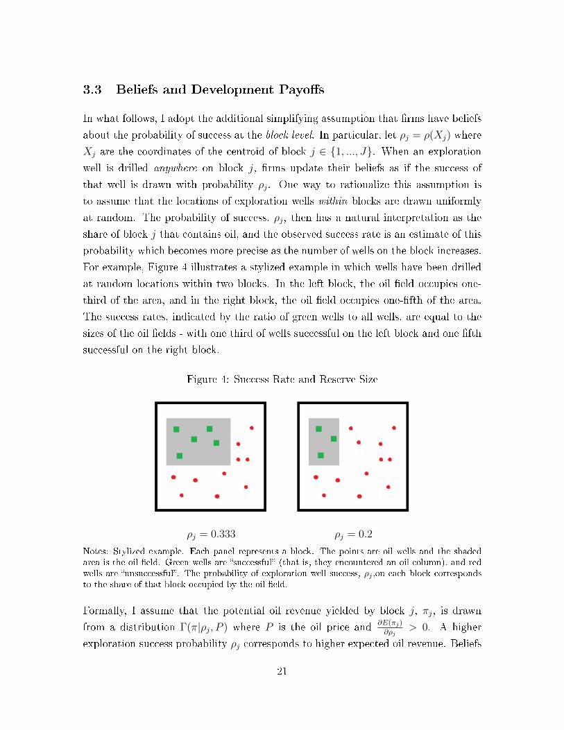
For example, Figure 4 illustrates a stylized example in which wells have been drilled

at random locations within two blocks. In the left block, the oil eld occupies one-

third of the area, and in the right block, the oil eld occupies one-fth of the area.

The success rates, indicated by the ratio of green wells to all wells, are equal to the

sizes of the oil elds - with one third of wells successful on the left block and one fth

successful on the right block.

Figure 4: Success Rate and Reserve Size

ρj = 0.333 ρj = 0.2

Notes: Stylized example. Each panel represents a block. The points are oil wells and the shadedarea is the oil eld. Green wells are successful (that is, they encountered an oil column), and redwells are unsuccessful. The probability of exploration well success, ρj ,on each block correspondsto the share of that block occupied by the oil eld.

Formally, I assume that the potential oil revenue yielded by block j, πj, is drawn

from a distribution Γ(π|ρj, P ) where P is the oil price and∂E(πj)

∂ρj> 0. A higher

exploration success probability ρj corresponds to higher expected oil revenue. Beliefs

21

about exploration well success G(ρ) then imply beliefs about the potential oil revenue

on block j given by:

Γj(π|G,P ) =

∫Γ(π|ρj, P )dG(ρ). (5)

This interpretation of block-level success rates is supported by positive relationship

between the realized exploration success rate and estimated oil reserves on developed

blocks, illustrated by Figure 2. Note that the assumption that probability of success

is a primitive feature of a block and within-block location choice is random implies

that the realized success rate on a block should be constant over time. This might not

be true if, for example, rms continue to drill near previous successful wells within

the block. I test this implication in Appendix Table A5. I present the results of

regressions that show that within blocks, the success rate is not signicantly higher

or lower for later wells than for earlier wells. That is, the eect of the well sequence

number on success probability is not statistically signicant. This is consistent with

a model in which within-block well locations are drawn at random.

4 Descriptive Evidence

The estimated model of beliefs suggests that there is high degree of correlation be-

tween well outcomes on neighboring blocks. This spatial correlation is estimated

from data on well outcomes at dierent locations. In this section, I use data on rms'

drilling decisions to test whether rm behavior is consistent with the estimated model

of rational beliefs.

I provide evidence that rms respond to the results of past wells, both their own

wells and those of other rms, in a way that is consistent with the estimated spatial

correlation of well results. I also provide direct evidence of free riding by showing

how drilling behavior changes when the spatial arrangement of licenses changes.

4.1 Exploration Drilling Patterns

The estimated spatial correlation illustrated by Figure 3 suggests that rms should

make inferences across space based on past well results. I test this prediction using

data on rm behavior. Let Sucjdot be the cumulative number of successful wells

22

drilled on blocks distance d from block j before date t by rms o ∈ f,−f, where −findicates all rms other than rm f . Failjdot is analogously dened as the cumulative

number of past unsuccessful wells. I estimate the following regression specication

using OLS:

Explorefjt = αf + βj + γt +∑d

∑o∈f,−f

gdo (Sucjdot, Failjdot)) + εfjt. (6)

Where gdo is a exible function of cumulative successful and successful well counts

for wells of type (d, o). Explorefjt is an indicator for whether or not rm f drilled an

exploration well on block j in month t. Notice that the specication includes rm,

block, and month xed eects. This means that the eects of past wells are identied

by within-block changes in the set of well results over time, and not by the fact that

some blocks have higher average success rates than others and these blocks tend to

be explored more.

Figure 5: Response of Drilling Probability to Cumulative Past Results

0.0

10

.11

−0

.01

−0

.1−

1

Eff

ect

of

Pa

st

We

ll O

utc

om

es O

n P

rob

ab

ility

of

Exp

lora

tio

n (

Pe

rce

nta

ge

Po

ints

, L

og

Sca

le)

0 1−3 4−6Distance (Blocks)

Same Firm, Successful Same Firm, Unsuccessful

Other Firm, Successful Other Firm, Unsuccessful

Notes: Points are the estimated marginal eect of each type of past well on Explorefjt from thespecication given by equation 6 where gdo(·) is quadratic in each of the arguments. Marginal eectsare computed for the rst well of each type. Error bars are 95% condence intervals computed usingstandard errors clustered at the rm-month level. Sample includes block-months in the relevantregion between 1970 and 1990. I drop observations from highly explored regions where the numberof nearby own wells (those on 1st and 2nd degree neighboring blocks) is above the 90th percentileof the distribution in the data.

23

Figure 5 records the estimated marginal eect of the rst well of each type on the

probability of susequent exploration. I include three distance bands in the regression

- wells on the same block, those 1-3 blocks away, and those 4-6 blocks away. Solid

red circles indicate the eect on the probability of rm f drilling an exploration well

on block j of an additional past successful well drilled by rm f at each distance.

Hollow red circles record this eect for unsuccessful past wells drilled by rm f . The

results indicate that additional successful wells on the same block and 1-3 blocks away

signicantly increase the probability of subsequent exploration, and an additional

unsuccessful wells signicantly decrease the probability of subsequent exploration.

The eect of an additional same rm, same block well is approximately 120% of the

mean of the dependent variable, Explorefjt, which is 0.0161, and the size of the eect

is roughly equal for successful and unsuccessful wells. The magnitude of the eect

decreases with distance. Notice that the y-axis of Figure 5 is on a log scale. The eect

of past wells at a distance of 1-3 blocks is about 10% of the eect of past same-block

wells. The eect at distances of 4-6 blocks is on the order of 1% of the same-block

eect and is not statistically signicant.

Blue squares indicate the eect of past wells drilled by other rms on rm f 's prob-

ability of exploration. The eects are of the same sign but have magnitudes between

20% and 50% of the same-rm well eects. As with the same-rm eects, the other-

rm eects diminish with distance and lose statistical signicance at distances of 4-6

blocks.12

These results suggest that rm's decisions about where to drill depend on the results

of nearby past wells, both their own wells and those of their rivals. The probability

of drilling on block j responds both to the results of past wells on block j as well as

to the results of wells on nearby blocks, suggesting that rms make inferences across

space at distances consistent with the spatial correlation of well results illustrated by

Figure 3, with the size of the drilling response declining with distance. Exploration

probability is also more responsive to own-rm exploration results than to other-rm

exploration results, suggesting that information ow across rms is imperfect.13

12Since the regression includes block xed eects, the eect of other rm wells on the same blockcomes from variation in the number of wells over time when multiple rms hold licenses on the sameblock. See Section 2.2 for discussion of how I assign blocks to rms.

13One potential concern is that these results could be explained by the arrival over time of publicinformation that is independent of drilling results and is correlated over space. To test of whether

24

In Appendix Table A6 I report analogous results for dierent sub-periods of the

data. These results indicate that the ratio of the eect of wells 1-3 blocks away to

the eect of wells on the same block is relatively constant over time. Firms do not

appear to have been systematically over- or under-extrapolating across space during

early exploration. This nding is consistent with the assumption that the rms are

learning about the location of oil, not about the true value of the spatial covariance

parameter ` which I assume is known to rms ex-ante.

To test directly whether rm behavior responds to changes in beliefs, I regress rm

exploration decisions on model-implied posteriors. Since exploration wells generate

information, and their value is in informing rms' future drilling decisions, a natural

hypothesis is that the probability of drilling an exploration well should be increasing

in the expected information generated by that well. For instance, the rst exploration

well drilled on a block should be more valuable than the tenth because its marginal

eect on beliefs is greater.

I compute the model-implied posterior beliefs for each block j, each month t, based

on all wells drilled before that month according to the Bayesian updating rule (4).14

I obtain Et(ρj), the posterior mean, and V art(ρj), the posterior variance of beliefs

about the probability of success on block j, ρj. To measure the expected information

gain of an additional well I obtain the expected Kulback-Leibler divergence, KLj,t,

between the prior and posterior distributions following an additional exploration well

for each (j, t).15

Column 1 of Table 3 records the coecients from a regression of KLj,t on the com-

puted posterior variance and a quadratic in posterior mean at (j, t). There is an

inverse u-shaped relationship between expected KL divergence and Et(ρj) that is

maximized when Et(ρj) = 0.48. This reects the classic result in information theory

the information generated by past wells is driving these results, I use the fact that the condentialityperiod on exploration data expires 5 years after a well is drilled. In Appendix Figure A5 I show thatmoving an successful other-rm well back in time by more than 6 months has a positive and signicanteect on the probability of exploration. The eect is greatest for wells close to the condentialitycuto, drilled between 4.5 and 5 years ago. For wells that are older than 5 years, there is nosignicant eect, consistent with the outcomes of these wells already being public knowledge.

14In this section, I compute beliefs as if all rms observe the results of all other rms' explorationwells. This assumption is relaxed in the structural model developed in Section 5.

15The KL divergence is a measure of the dierence between two distributions. It can be interpretedas the information gain when moving from one distribution to another (see Kullback, 1997). SeeAppendix B for details.

25

(see for example MacKay, 2003) that the information generated by a Bernoulli ran-

dom variable is maximized when the probability of success is 0.5. There is a positive

relationship between V art(ρj) and KLjt. It is clear that as variance goes to 0, the

change in beliefs from an additional well will also go to 0.

The second column of Table 3 presents estimated coecients from a regression of

Explorefjt on V art(ρj), a quadratic in Et(ρj), and (f, j) level xed eects. Note

that the coecients follow the same pattern as those in the rst column: rms are

less likely to drill exploration wells on blocks with very high or very low expected

probability of success, and are more likely to drill exploration wells on blocks with

higher variance in beliefs. Firm behavior aligns closely with the theoretical relation-

ship between moments of the posterior beliefs and the expected information generated

by exploration wells. This is conrmed by the results in column 3, which presents

the estimated positive and signicant coecient from a regression of Explorefjt on

KLjt. The fourth column shows that development is more likely on blocks with high

mean and low variance beliefs, consistent with the correlation between exploration

well success and oil reserves illustrated by Figure 2.

Table 3: Response of Drilling Probability to Posterior Beliefs and License Distribution

Dependent Variable: KL Divergence Exploration Well Develop Block

Posterior Mean 0.420*** 0.285*** . 0.006*

(0.009) (0.070) . (0.003)

Posterior Mean2 -0.458*** -0.252** . .

(0.013) (0.099) . .

Posterior Variance 0.081*** 0.023*** . -0.002**

(0.000) (0.008) . (0.001)

KL Divergence . . 0.284***

. . (0.080)

Own Share Nearby Blocks . 0.027** 0.028** 0.000

. (0.011) (0.011) (0.001)

R2 0.972 0.120 0.119 0.093

N 73,493 73,493 73,493 73,493

Firm-Month and Block FE No Yes Yes Yes

Notes: Standard errors clustered at the rm-month level. Mean, variance, and KL divergence ofposterior beliefs computed for each (f, j, t) as if all wells drilled by all rms up to month t − 1are observed. Sample is all undeveloped rm-block-months in the relevant region,. *** indicatessignicance at the 99% level. ** indicates signicance at the 95% level. * indicates signicance atthe 90% level. Sample includes block-months in the relevant region between 1970 and 1990.

26

The nal row of Table 3 reports coecients on the share of nearby blocks belonging

to the same rm as block j. The results indicates that a rm is more likely to ex-

plore when a larger share of the surrounding blocks are owned by that rm. There is

no signicant eect of the nearby license share on the development decision. These

results are consistent with information spillovers across blocks driving rms' explo-

ration decisions. Since the information generated by an exploration well on block j

is informative about nearby blocks, a rm learns more about the distribution of oil

on its own blocks when it holds licenses on more of the block surrounding block j.

On the other had when other rms hold more of the blocks surrounding block j, then

a rm may have a greater incentive to delay exploration and learn from other rms'

results.

In the Appendix, I present additional results consistent with these strategic eects

of information spillovers. Appendix Table A7 presents results indicating that rms'

exploration rates fall signicantly after licensing rounds in which more new licenses are

issued to other rms on nearby blocks. In Appendix Figures A6 and A7, I reproduce a

result from Hendricks and Porter (1996), who showed that the probability of drilling

an exploration well on unexplored tracts in the Gulf of Mexico increased near the

drilling deadline imposed by the tract lease. The authors argue that this delay until

the end of the lease term is evidence of a free riding incentive. I show that the same

pattern obtains on North Sea blocks when the drilling deadline (which, as discussed

in Section 2, is not as strict as the deadline imposed in the Gulf) approaches. I also

show that this pattern is present for license blocks with a large number of other rm

license nearby, but is not present for blocks that are far from other rm licenses.

5 An Econometric Model of Optimal Exploration

To measure the extent to which information externalities aect industry surplus, I

estimate a structural econometric model of the rm's exploration problem in which I

assume that rm beliefs follow the logistic Gaussian process model of Section 3.2. I set

up the rm's problem by specifying a full information game in which rms observe the

results of all wells. Motivated by the empirical ndings described in Section 3, I then

extend the model to one of asymmetric information in which rms do not observe

the results of other rms' wells with certainty. I describe an assumption on rm

27

beliefs and specify an equilibrium concept that makes estimation of the asymmetric

information game feasible.

5.1 Full Information

I start by specifying a full information game played by a set of rms F . Firms are

indexed by f , discrete time periods are indexed by t, and blocks are indexed by j. J

is the set of all blocks. Jft ⊂ J is the set of undeveloped blocks on which rm f holds

drilling rights at the beginning of period t. J0t ⊂ J is the set of undeveloped blocks

on which no rm holds drilling rights at the beginning of period t. Pt is the oil price.

Exploration wells are indexed by w, and each well is associated with an outcome

s(w) ∈ 0, 1, a block j(w), a rm f(w), and a drill date t(w). The set of all locations

and realizations of exploration wells drilled on date t is given by Wt = (j(w), s(w)) :

t(w) = t.

The rm's prior beliefs about the probability of exploration well success on each block

are given by the logistic Gaussian process G0 dened in Section 3.1. Gft is rm f 's

posterior at the beginning of period t. Under the assumption of full information rms

observe the results of all wells, so Gft+1 = B(Gft,Wt) and Gft = Gt for all rms

f ∈ F , where B(·) is dened in equation 4.

The industry state at date t is described by

St = Gt, Jftf∈F∪0, Pt. (7)

Each period, the rm makes two decisions sequentially. First, in the exploration

stage, it selects at most one block on which to drill an exploration well. Then, in the

development stage, it selects at most one block to develop.

Drilling an exploration well on block j incurs a cost, c(j,St)− εftj. Developing blockj incurs a cost κ(j,St)− νftj. εftj and νfjt are private information cost shocks drawn

iid from logistic distributions with variance parameters σε and σν . Developing block

j at date t yields a random payo πjt. Firms' beliefs about the distribution of payos

on block j are Γj(π|Gt, Pt), dened in equation 5.

The timing of the game is as follows:

Exploration Stage

28

1. Given state St, each rm f observes a vector of private cost shocks εft.

2. Firm f chooses an exploration action, aEft ∈ Jft ∪ 0. If aEft 6= 0, then rm f

incurs an exploration cost.

3. Exploration well results Wt are realized.

4. The industry state evolves to S ′t = Gt+1, Jftf∈F∪0, Pt.

Development Stage

1. Given state S ′t , each rm f observes a vector of private cost shocks νft.

2. Firm f chooses a development action, aDft ∈ Jft ∪ 0. If aDft 6= 0, then rm f

incurs a development cost.

3. If aDft = j then the rm f draws oil revenue πjt.

4. The industry state evolves to St+1 = Gt+1, Jft+1f∈F∪0, Pt+1.16

State variables evolve at the end of the development stage as follows. I assume that

log oil price follows an exogenous random walk, so Pt+1 = exp(log(Pt) + ζt) where

ζt ∼ N(0, σζ). I assume that rm licenses on undeveloped blocks are issued and

surrendered according to an exogenous stochastic process dened by probabilities

P (j ∈ Jft+1|Jgtg∈F∪0, aDft). Developed blocks are removed from rms' choice sets,

so P (j ∈ Jft+1|aDft = j) = 0 and P (j ∈ Jft+1|j /∈ ∪Jgtg∈F∪0) = 0. This as-

sumption eliminates any strategic consideration in the timing of drilling with respect

to regulatory deadlines, the announcement of new licensing rounds, and the rm's

decision to surrender a block.

16Note that I have assumed that rms do not update their beliefs based on the outcomes ofdevelopment decisions. Formally, this assumption means that although rms obtain revenues πj aftermaking development decisions, they do not observe πj . The assumption that rms do not updatetheir beliefs based on this realization is likely not unreasonable. In reality oil ow is obtainedfrom a reservoir over many years, and additional information about the true size of the eld isgradually obtained. Furthermore, since development platforms are very expensive, the informationvalue of development is unlikely to be pivotal to the development decision, and the marginal eectof information revealed by the development outcome is likely to be small since development takesplace only after extensive exploration.

29

The rm's continuation values at the beginning of the exploration and development

stages (before private cost shocks are realized) are described by the following two

Bellman equations:

V Ef (St) = Eεft

[max

aEt ∈Jft∪0

ES′t

[V Df (S ′t)|aEt ,St

]− c(aEt ,St) + εftj

](8)

V Df (S ′t) = Eνft

[max

aDt ∈Jft∪0

Eπ

aDt,St+1

[βV E

f (St+1) + πaDt |aDt ,S ′t

]− κ(aDt |S ′t) + νftj

].

Where β is the one period discount rate. The inner expectation in the exploration

Bellman equation is taken over realizations of the intermediate state S ′t, with respect

to the rm's beliefs Gt and beliefs about other rms' exploration actions. The inner

expectation in the development Bellman equation is taken over realizations of devel-

opment revenues πaD and realizations of next period's state variable St, with respect

to the rm's beliefs Gt+1 and beliefs about other rms' actions.

Dene choice specic ex-ante (before private cost shocks are realized) value functions

as,

vEf (aEt ,St) =ES′t[V Df (S ′t)|aEt ,St

]− c(aEt ,St)

vDf (aDt ,S ′t) =EπaDt

,St+1

[βV E

f (St+1) + πaDt |aDt ,S ′t

]− κ(aDt ,S ′t). (9)

I assume that εftj and νftj are distributed type I extreme value with standard devia-

tion parameters σε and σν , yielding conditional choice probabilities (CCPs):

P (aEf = j|St) =exp

(1σεvEf (j,St)

)∑

k∈Jft∪0 exp(

1σεvEf (k,St))

) . (10)

With a similar expression for the CCP of development action j, P (aDf = j|S ′t).

A Markov perfect equilibrium of this game is then dened by strategies aEf (S, ε)and aDf (S,ν) that maximize the rm's continuation value, conditional on the state

30

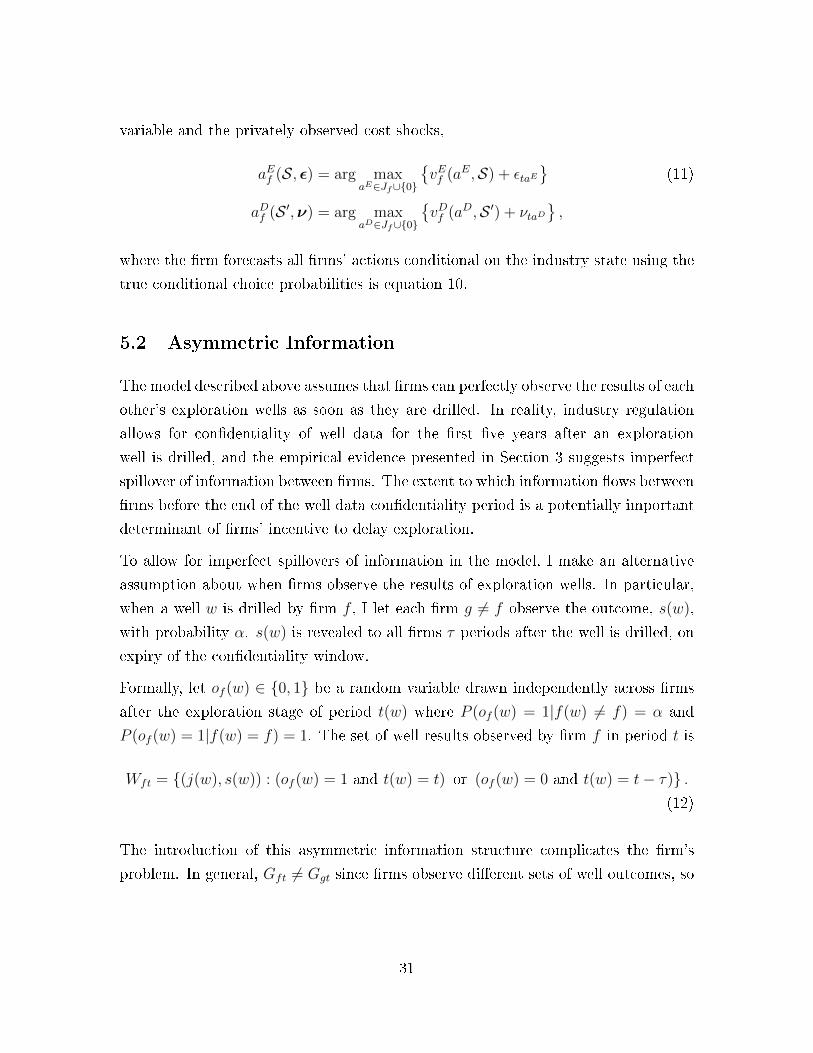
variable and the privately observed cost shocks,

aEf (S, ε) = arg maxaE∈Jf∪0

vEf (aE,S) + εtaE

(11)

aDf (S ′,ν) = arg maxaD∈Jf∪0

vDf (aD,S ′) + νtaD

,

where the rm forecasts all rms' actions conditional on the industry state using the

true conditional choice probabilities is equation 10.

5.2 Asymmetric Information

The model described above assumes that rms can perfectly observe the results of each

other's exploration wells as soon as they are drilled. In reality, industry regulation

allows for condentiality of well data for the rst ve years after an exploration

well is drilled, and the empirical evidence presented in Section 3 suggests imperfect

spillover of information between rms. The extent to which information ows between

rms before the end of the well data condentiality period is a potentially important

determinant of rms' incentive to delay exploration.

To allow for imperfect spillovers of information in the model, I make an alternative

assumption about when rms observe the results of exploration wells. In particular,

when a well w is drilled by rm f , I let each rm g 6= f observe the outcome, s(w),

with probability α. s(w) is revealed to all rms τ periods after the well is drilled, on

expiry of the condentiality window.

Formally, let of (w) ∈ 0, 1 be a random variable drawn independently across rms

after the exploration stage of period t(w) where P (of (w) = 1|f(w) 6= f) = α and

P (of (w) = 1|f(w) = f) = 1. The set of well results observed by rm f in period t is

Wft = (j(w), s(w)) : (of (w) = 1 and t(w) = t) or (of (w) = 0 and t(w) = t− τ) .(12)

The introduction of this asymmetric information structure complicates the rm's

problem. In general, Gft 6= Ggt since rms observe dierent sets of well outcomes, so

31

rm f 's state variable can now be written:

Sft = Gft, Jftf∈F∪0, Pt. (13)

In Markov perfect Bayesian equilibrium, each f must form beliefs about every other

rm g's beliefs, Ggt in order to forecast the next period's state. The history of rm

g's actions is informative about Ggt and about well outcomes unobserved by rm f .

Firm f should therefore update its beliefs based not only on observed outcomes, but

on the past behavior of other rms. For instance, if rm g drilled many exploration

wells on block j, this should signal to rm f something about the success probability

on that block, even if rm f did not observe the outcome of any of those wells directly.

In contrast to the full information game, this means that the entire history of drilling

and license allocations should enter the rm's state.

As discussed by Fershtman and Pakes (2012) the addition of these informationally

relevant but not payo relevant state variables makes estimating the asymmetric

information game and nding equilibria computationally infeasible. Because of these

diculties, dynamic games with asymmetric information have not been widely used

in empirical work. To make progress, I impose an equilibrium assumption on rms'

beliefs similar to Fershtman and Pakes' (2012) Experience Based Equilibrium (EBE)

approach. First, I dene a belief function that maps a rm's current information, Sf ,to perceived probabilities of other rms' actions.

Assumption A1: Firm f believes that at every period t the probability of a

new exploration well being drilled by a rm g 6= f on block j ∈ Jgt is given

by QE(Sft, g, j) ∈ [0, 1]. Likewise rm f believes that at every period t the

probability of rm g 6= f developing block j ∈ Jgt is QD(Sft, g, j) ∈ [0, 1].

Assumption A1 says that rms' beliefs are specied by functions QE and QD of

their current state Sft. For example, these functions could be the expected action

probabilities based on Bayesian posteriors about other rms' states. Notice that

although this assumption allows for Bayesian beliefs, it restricts the set of information

that rms can use to make forecasts about other rms' actions to the payo-relevant

state variables in equation 13. For instance, this assumption means that rm f

cannot make inferences about rm g's future actions based on the sequence of past

32

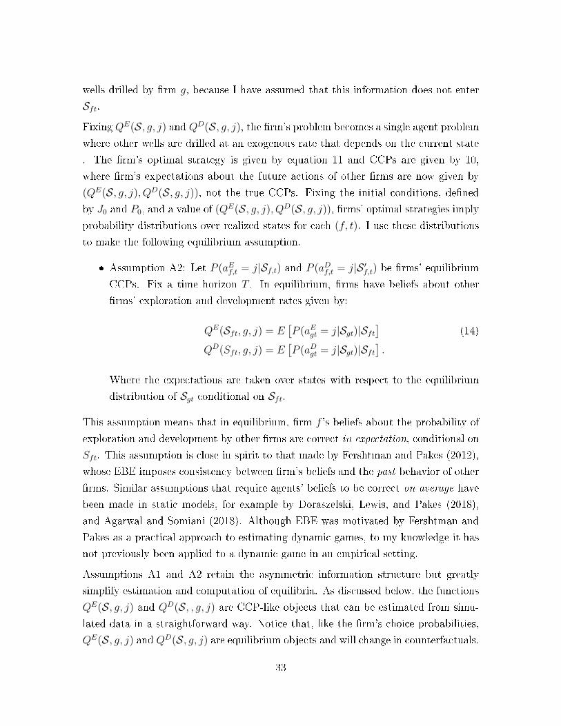
wells drilled by rm g, because I have assumed that this information does not enter

Sft.

Fixing QE(S, g, j) and QD(S, g, j), the rm's problem becomes a single agent problem

where other wells are drilled at an exogenous rate that depends on the current state

. The rm's optimal strategy is given by equation 11 and CCPs are given by 10,

where rm's expectations about the future actions of other rms are now given by

(QE(S, g, j), QD(S, g, j)), not the true CCPs. Fixing the initial conditions, dened

by J0 and P0, and a value of (QE(S, g, j), QD(S, g, j)), rms' optimal strategies imply

probability distributions over realized states for each (f, t). I use these distributions

to make the following equilibrium assumption.

Assumption A2: Let P (aEf,t = j|Sf,t) and P (aDf,t = j|S ′f,t) be rms' equilibrium

CCPs. Fix a time horizon T . In equilibrium, rms have beliefs about other

rms' exploration and development rates given by:

QE(Sft, g, j) = E[P (aEgt = j|Sgt)|Sft

](14)

QD(Sft, g, j) = E[P (aDgt = j|Sgt)|Sft

].

Where the expectations are taken over states with respect to the equilibrium

distribution of Sgt conditional on Sft.

This assumption means that in equilibrium, rm f 's beliefs about the probability of

exploration and development by other rms are correct in expectation, conditional on

Sft. This assumption is close in spirit to that made by Fershtman and Pakes (2012),

whose EBE imposes consistency between rm's beliefs and the past behavior of other

rms. Similar assumptions that require agents' beliefs to be correct on average have

been made in static models, for example by Doraszelski, Lewis, and Pakes (2018),

and Agarwal and Somiani (2018). Although EBE was motivated by Fershtman and

Pakes as a practical approach to estimating dynamic games, to my knowledge it has

not previously been applied to a dynamic game in an empirical setting.

Assumptions A1 and A2 retain the asymmetric information structure but greatly

simplify estimation and computation of equilibria. As discussed below, the functions

QE(S, g, j) and QD(S, , g, j) are CCP-like objects that can be estimated from simu-

lated data in a straightforward way. Notice that, like the rm's choice probabilities,

QE(S, g, j) and QD(S, g, j) are equilibrium objects and will change in counterfactuals.

33

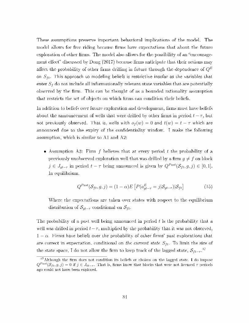
These assumptions preserve important behavioral implications of the model. The

model allows for free riding because rms have expectations that about the future

exploration of other rms. The model also allows for the possibility of an encourage-

ment eect discussed by Dong (2017) because rms anticipate that their actions may

aect the probability of other rms drilling in future through the dependence of QE

on Sft. This approach to modeling beliefs is restrictive insofar as the variables that

enter Sf do not include all informationally relevant state variables that are potentially

observed by the rm. This can be thought of as a bounded rationality assumption

that restricts the set of objects on which rms can condition their beliefs.

In addition to beliefs over future exploration and development, rms must have beliefs

about the announcement of wells that were drilled by other rms in period t− τ , butnot previously observed. That is, wells with of (w) = 0 and t(w) = t − τ which are

announced due to the expiry of the condentiality window. I make the following

assumption, which is similar to A1 and A2:

Assumption A3: Firm f believes that at every period t the probability of a

previously unobserved exploration well that was drilled by a rm g 6= f on block

j ∈ Jgt−τ in period t − τ being announced is given by QPast(Sft, g, j) ∈ [0, 1].

In equilibrium,

QPast(Sft, g, j) = (1− α)E[P (aEgt−τ = j|Sgt−τ )|Sft

](15)

Where the expectations are taken over states with respect to the equilibrium

distribution of Sgt−τ conditional on Sft.

The probability of a past well being announced in period t is the probability that a

well was drilled in period t−τ , multiplied by the probability that it was not observed,

1 − α. Firms have beliefs over the probability of other rms' past explorations that

are correct in expectation, conditional on the current state Sft. To limit the size of

the state space, I do not allow the rm to keep track of the lagged state, Sft−τ .17

17Although the rm does not condition its beliefs or choices on the lagged state, I do imposeQPast(Sft, g, j) = 0 if j ∈ J0t−τ . That is, rms know that blocks that were not licensed τ periodsago could not have been explored.

34

6 Estimation & Identication

6.1 Parameterization

I use the monthly Brent crude price inated to 2015 dollars using the UK GDP deator

to measure the oil price. For years before 1980 where the Brent price is unavailable I

use projected values from a regression of Brent on the West Texas Intermediate price.

I let a period be one month, and set the number to periods after which well outcomes

are made public to τ = 60.18 This corresponds to the 5 year condentiality period

imposed by the regulator. I set the one month discount rate to β = 0.992, which

corresponds to a 10% annual discount.

To account for heterogeneity in exploration and development rates across blocks with

similar exploration well outcomes, I allow costs to depends on observable rm-block

characteristics according to equation 16.

c(j,Sft) = c0 + c1Xcjft (16)

κ(j,Sft) = κ0 + κ1Xκjft.

Xcjft includes the distance of block j from Aberdeen (the North Sea's major supply

harbor), an indicator for whether rm f has observed the outcome of at least one

well on block j in the past, and the variance of f 's beliefs Gft about the probability

of exploration well success on block j. Xκjft includes only the variance of f 's beliefs

Gft on block j.19

I augment the rm's state variable 13 with these characteristics, which are either

xed at the level of block j or functions of the rm's information about exploration

wells 12. The dependence of exploration and development costs on past exploration

and the variance of rm's beliefs models the fact that more heavily explored areas

are likely to be better understood in terms of geology and optimal drilling technology

18The choice of a one month period imposes an implicit capacity constraint - each rm can chooseat most one block to explore and one block to develop each month. In practice, in 94% of (f, t)observations where exploration takes place, only one exploration well is drilled. I never observe morethan one block developed by the same rm in the same month. In my detailed discussion of theestimation routine in Appendix C, I describe how I deal with observations where there are multipleexploration wells in a month.

19I do not adopt a richer specication of development costs because of the relatively small numberof development actions in the data (44).

35

(see for example Covert (2015) and Steck (2018) on learning about location-specic

drilling technology). This rationalizes

The model parameters are therefore θ1, θ2, α, σζ, where θ1 = µ, ω, ` are the pa-

rameters of the rm's beliefs dened in Section 3, θ2 = c0, c1, κ0, σc, σκ are the costparameters, α is the probability of observing another rm's well outcome before it is

made public, and σζ is the variance of innovations to the oil price random walk. Other

objects to be estimated are the transition probabilities of the license issuing process

P (j ∈ Jft+1|Jt, Jgt∀g∈F ), the distribution of development prots, Γ(π; ρj, Pt), and

rm beliefs about other rms' actions, QE, QD, and QPast.

6.2 Estimation

Parameters θ1 are taken from the estimation procedure described in Section 4.1. I

estimate σζ with the variance of monthly changes in the log oil price. I estimate

Γ(·) using data on realized oil ows from all developed wells. I detail this part of

estimation in Appendix C.4. Probabilities P (j ∈ Jf,t+1|Jt, Jg,t∀g∈F ) that are used

by rms to forecast the evolution of license assignments are estimated using a logit

regression of the licenses issued in period t + 1 on the period t license assignment. I

detail this part of estimation in Appendix C.5.

The remaining parameters, θ2 and α, are estimated using a two step conditional choice

probability method related to those described by Hotz, Miller, Sanders and Smith

(1994) and Bajari, Benkard and Levin (2007). In the rst step, I obtain estimates of

the conditional choice probabilities (CCPs) given by equation 10 and the parameter

α. First step estimates of the CCPs are then used to simulate data which I use to

estimate the belief functions QE, QD, and QPast.

Using the estimated CCPs and belief functions, I compute the rm's state-specic

continuation values (8) as functions of the remaining parameters θ2 by forward sim-

ulation. I then nd the value of θ2 that minimizes the distance between the rst

step estimates of the CCPs and the choice probabilities implied by the simulated

continuation values. I describe this two step procedure in detail in Appendix C.

36

6.2.1 Estimation of Conditional Choice Probabilities

If the state variable were observable in the data, then CCPs P (aEf = j|S) and P (aD =

j|S) could be estimated directly using the empirical choice probability conditional on

the state. However, the asymmetric information structure of the model means that

the true state is not observed by the econometrician. In particular, the econometrician

knows the outcome of every well, but does not know which outcomes were observed

by each rm. Formally, the data does not include the vector of that records which

other-rm well outcomes were observed by rm f . Dierent realizations of of imply

dierent states through the eect of observed well outcomes on Gft. The data is

therefore consistent with a set of possible states Sf for each rm.20

To recover CCP estimates, observe that dierent values of the parameter α dene

distributions P (Sf |Sf , α) over the elements of Sf . For example, suppose at date t

there was one other-rm well w that may have been observed by rm f . The data is

consistent with two possible states: let S1ft be the state if of (w) = 1 and S0

ft be the

state if of (w) = 0. From the econometrician's perspective, P (S1ft|S1

ft,S0ft, α) = α.

I provide a formal denition of the distribution P (Sf |Sf , α) in Appendix C.

Given this distribution over states, the likelihood of a sequence of exploration and

development choice observations is:

Lf =∑Sf∈Sf

T∏t=1

∏j∈Jft∪0

P (aE = j|Sf )1(aEft=j)P (aD = j|Sf )1(a

Dft=j)

P (Sf |Sf , α)

.(17)

I maximize this likelihood to obtain estimates of the conditional choice probabili-

ties P (aEf = j|S) and the information spillover parameter, α, which controls the

probability weight placed on each of the dierent states Sf ∈ Sf that could have

obtained given the data. To ease computation, I allow α to take values on a grid

[0, 0.01, ..., 0.99, 1]. Since the state variable is high dimensional, I use the logit struc-

ture of P (aEf = j|S) implied by equation 10 and approximate the choice specic value

function for each alternative with a linear equation in elements of the state variable.

For the exploration choice, this approximation to the state variable includes a third

order polynomial in the mean and variance of beliefs Gft on each block, interactions

20More precisely, and element of Sf is a particular sequence of rm-f states Sf = SftTt=1. See

Appendix C for a formal denition of Sf .

37

with the oil price, and counts of nearby own- and other-rm licenses for each block.

Full details are provided in Appendix C. In approximating a high dimensional state

variable with lower dimensional statistics I follow much of the applied literature that

estimates dynamic discrete choice models with conditional choice probability meth-

ods. For example, see Ryan and Tucker (2011), Collard-Wexler (2013), and Agarwal

et al. (2020).

6.2.2 Estimation of Belief Functions

The estimated choice probabilities and spillover parameter α can be used to simulate

drilling histories for the entire market. Under the assumption that CCPs reect

equilibrium policy functions, the data generated by these simulations is drawn from

the equilibrium distribution of states. These simulations can be used to estimate

empirical analogues, QE(Sft, g, j), QD(Sft, g, j), and QPast(Sft, g, j), of equations 14and 15, since in the simulated data each rm's state is fully observed.

I parameterize QE(Sft, g, j) using a linear equation in elements of Sft similar to that

used to estimate the CCPs. I run a logit regressions of other rms' exploration choices

on rm f 's state, pooling data across all rms. QD(Sft, g, j), and QPast(Sft, g, j) areestimated analogously. Details on this procedure are provided in Appendix C.2.

Firm f 's estimated beliefs about the actions of other rms are therefore set equal

to expected actions under equilibrium play, conditional on state Sft. This approachto estimating equilibrium beliefs extends the logic of the CCP approach of Hotz

and Miller (1993). If equilibrium policy functions can be recovered directly from

the data, then under assumptions A1-A3, equilibrium beliefs can be recovered by

simulating data using these policy functions. This approach does not require solving

for optimal policy functions or equilibrium beliefs using value function iteration and

is an alternative to the reinforcement learning algorithm suggested by Fershtman and

Pakes (2012).

38

6.3 Identication

6.3.1 Identication of CCPs

The rst step of the estimation procedure recovers the parameter α and conditional

choice probabilities P (a = j|S) at each state S from data in which each observation

is consistent with a set of states S. The model's information structure means these

objects are separately identied despite the fact that the econometrician does not

observe the full state. In particular, I claim that the list of choice probabilities

P (a = j|S) for each set of states S that it is possible to observe in the data can

be inverted to uniquely identify choice probabilities conditioned on the unobserved

states P (a = j|S) and the information spillover parameter α.

To illustrate identication, consider the following simplied example. Suppose that

a state is described by a triple, S = (suc, fail, unobs), where suc is the number

of successful wells observed, fail is the number of unsuccessful wells observed, and

unobs is the number of wells with unobserved outcomes. Consider data that contains

observations consistent with the following sets of states:

SA = (1, 0, 0) (18)

SB = (0, 1, 0)

SC = (1, 0, 0), (0, 0, 1)

SD = (0, 1, 0), (0, 0, 1).

SA and SB are observed by the econometrician when there is one own-rm well out-

come. The econometrician then knows the state with certainty since the rm always

observes their own well outcome. SC and SD are observed by the econometrician

when there is one other-rm well outcome. In this case, the econometrician knows

whether the well was successful or unsuccessful, but not whether the rm observed

the outcome or not. Given a value of the parameter α, choice probabilities conditional

39

on the observed set of states can be written as:

P (a = j|SA) = P (a = j|S = (1, 0, 0)) (19)

P (a = j|SB) = P (a = j|S = (0, 1, 0))

P (a = j|SC) = αP (a = j|S = (1, 0, 0)) + (1− α)P (a = j|S = (0, 0, 1))

P (a = j|SD) = αP (a = j|S = (0, 1, 0)) + (1− α)P (a = j|S = (0, 0, 1)).

The left hand side of each equation is a probability that is observable in the data.

Notice that there are four equations and four unknowns - three conditional choice

probabilities and the parameter α. The rst two equations yield estimates of P (a =

j|S = (1, 0, 0)) and P (a = j|S = (0, 1, 0)) directly. Rearranging the third and fourth

equations yields:

α =P (a = j|SC)− P (a = j|SD)

P (a = j|SA)− P (a = j|SB). (20)

This says that α is identied by the dierence between how much the rm responds

to other rm wells (the numerator) and how much the rm responds to its own wells

(the denominator). As documented in Figure 5, rms' exploration choices respond

more to the results of their own wells than to those of other rm wells, implying

0 < α < 1. P (a = j|S = (0, 0, 1)) is then identied by the level of P (a = j|SC) or

P (a = j|SD).

This identication argument relies on two features of the model's information struc-

ture. First, the belief updating rule (4) treats own-rm and other-rm well results

identically. This means that we can use the rm's response to their own wells to infer

how they would have responded if they had observed another rm's well. For exam-

ple, P (a = j|S = (1, 0, 0)) enters both the rst and third equation in (19). Second, if

rm f does not observe the outcome s(w) of well w at date t, then the s(w) does not

enter Sft. This means that if a well was not observed, then the rm's actions should

not depend on the well's outcome. That is, the second terms of the third and fourth

equation in (19) are identical. Relaxing either assumption would break identication

by introducing an extra free parameter.

This argument extends to states with multiple well results and well results at dierent

distances and dates. In particular for states with n wells there are always at least

as many equations as unknowns in the n well analogue of (19). This means that the

40

number of observable sets of states S, which correspond to equations, is always at

least one greater than the number of true states S. In Appendix D I provide a proof

that shows, in general, how P (a = j|S) can be identied from observable quantities

for any S. In practice, additional identication comes from the approximation of the

state variable which smooths choice probabilities across states and allow extrapolation

to states not observed in the data.

This approach to identication exploits a dierent source of variation than existing

literature on the identication of unobserved heterogeneity in dynamic discrete choice

(Berry and Compiani, 2021). Kasahara and Shimotsu (2008) show that mixture

models with persistent rm types are identied by time series variation within each

rm. Estimation of a model with this type of persistent unobservable heterogeneity

can be achieved using the iterative expectation-maximization procedure proposed by

Arcidiacono and Miller (2011). In contrast, my approach to identication relies on

cross-sectional variation in the econometrician's information about the rm's state

and the mixture distribution over possible information states, and estimation of the

CCPs and mixture parameter α is performed in a single step.21

6.3.2 Identication of Cost Parameters

The cost parameters are estimated in the second step of estimation, which minimizes

the distance between the rst step CCPs and model-predicted choice probabilities,

detailed in Appendix C. Intuitively, cost parameters c0 and κ0 are identied by the

average probability of exploration and development. Lower average probability of

drilling is rationalized by higher costs. Cost parameters c1 and κ1 are identied by

the extent to which the probability of drilling varies with observable characteristics

Xcjft and Xκ

jft. Additional identifying variation comes from the dierence in the

response of drilling probability to nearby own-rm and other-rm licenses. Higher

exploration drilling costs, c0, imply that rms have more of an incentive to free ride

and should have a lower exploration probability when the surrounding blocks are

owned by other rms than when they are owned by the same rm.

The exploration variance parameter σε is identied by the extent to which rms are

21This suggests that it may be possible to identity and estimate a model with both unobservedasymmetric information and persistent unobserved rm types by combining these two sources ofvariation.

41

more likely to explore blocks for which the expected future revenue stream condi-

tional on exploration is higher. The development variance parameter σν is similarly

identied. To see this, notice that 1σε

multiplies the choice specic continuation value

vEf (j,St) in equation 10, and the sum of future revenue enters linearly in the rm's

continuation value.22 As the variance of cost shocks becomes large, the probability of

any choice j ∈ Jft ∪ 0 tends to 1|Jft|+1

.

Finally note that, as discussed by Bajari, Benkard, and Levin (2007), the two step

procedure obtains consistent estimates of the model parameters if the data is gener-

ated by a single equilibrium. I assume this here since I cannot guarantee that there

is a unique equilibrium of the asymmetric information game.

7 Results

7.1 Estimates

Appendix Table A1 reports coecients from the estimated conditional choice prob-

abilities (CCPs) P (aE = j|S) and P (aD = j|S). The coecients are broadly as

expected. The probability of exploration is maximized when the expected probability

of success is around 0.5 and falls as the expected success probability approaches 1 or

0, in line with the descriptive results recorded in Table 3. Development probability

is increasing in expected probability of success and decreasing in variance, also con-

sistent with the descriptive results. Exploration probability is also increasing in the

number of nearby own-rm licenses and decreasing in the number of nearby other-

rm licenses, consistent with the presence of cross-block information spillovers and a

free riding incentive.

Table 4 reports estimated model parameters. The spillover parameter α which is

estimated simultaneously with the CCPs indicates that rms behave as if they observe

the results of 71% of other rm wells before they are made public. This nding is

in line with the descriptive results reported in Figure 5, which suggest imperfect

information spillover across rms.

Cost parameters are reported in billions of 2015 dollars. As expected, exploration

costs are lower after the rst exploration well on a block, and increasing in the variance

22See equation 30 in Appendix C.

42

Table 4: Parameter Estimates

Parameter Estimate SE Parameter Estimate SE

Information Spillover Development Cost

α 0.71 0.079 Constant 4.136 1.502

Variance of Beliefs 5.387 1.945

Exploration Cost σκ 0.913 0.335

Constant 0.719 0.172

Ever Explored 0.001 0.001 Oil Price Process

Variance of Beliefs 0.565 0.080 σξ 0.078 0.002

σc 0.323 0.056

Average Realized Costs

E(c(j,Sft)|aEt = j) 0.033 E(κ(j,Sft)|aEt = j) 1.651

Notes: Cost parameters are in billions of 2015 dollars. Standard error of α is computed using theinverse Hessian of the likelihood function given by equation 17 at the estimated parameter values.Standard error of σ2

ξ is computed using the fourth centered moment of month to month changes inlog price. Standard errors for the remaining (cost) parameters are computed using bootstrap drawsfrom the rst step CCP estimates. Average realized costs are computed by simulating esplorationand development behaviorusing the estimated rst step CCPs and taking the average realzied costs,including the cost shocks, ε and ν, over 10 simulations.

of rms' beliefs. Similarly, development costs are increasing in the variance of rms'

beliefs. The last row of Table 4 records average realized costs including the cost shocks

ε and ν computed from simulations. The average marginal cost of an exploration well

is $33 million. The average marginal cost of development is $1.6 billion. These average

realized costs are close to estimates of the capital costs of exploration and development

from auxiliary data on capital expenditure provided by the regulator that was not

used in estimation. The average capital expenditure per exploration well from this

auxiliary data is $20.9 million. The capital expenditure per development platform is

$1.26 billion.

To examine the t of the model to the data, I simulate the model from 1964 to

1990. Simulations are generated by drawing an action for each rm, each month,

and updating rms beliefs based on the observed results. For each month, I set the

distribution of licenses Jftf∈F and the oil price Pt equal to the truth. I use mean

values of the posterior success probability recorded in Figure A4, which is estimated

using the true outcomes of all wells drilled before 1990, to draw exploration well

outcomes and development revenue.

43

Table 5 records statistics on rm activity from the data and two simulations. The

rst column records the total the number of exploration wells, blocks developed,

blocks explored, and the average number of exploration wells drilled on developed and

undeveloped blocks from the data. The second column records the average of these

statistics over 40 simulations of the model using the rst step CCPs, P (aE = j|S) and

P (aD = j|S), to draw rm actions. Since the CCPs are estimated directly from the

data, it is not surprising that the total number of exploration wells drilled and blocks

developed in these simulations match the data reasonably closely. The mismatch

between the data and these simulations is likely due to the approximation to the

state variable used in the rst step of the estimation procedure.

Table 5: Model Fit

Data Simulation

First Step Probabilities Equilibrium Probabilities

Exploration Wells 1441 1414.9 1394.2Blocks Developed 44 39.8 37.0Exp. Wells/Dev. 32.068 35.550 37.681

Notes: Data column excludes multiple wills on same block on same date Column 1 records statisticsfrom the data covering 1964-1990 for the relevant region. Columns 2 and 3 are averages over 40simulations that cover 1964-1990. For each month the assignment of blocks to rms and the oilprice in the simulations are set at their realized values. Simulations in column 2 draw rm actionsusing the rst step estimates of the conditional choice probabilities. Well outcomes and developmentrevenue are drawn from the estimated gaussian process. Simulations in column 3 use equilibriumconditional choice probabilities at the estimated parameter values.

The third column records the average of these statistics over 40 simulations of the

model using approximate equilibrium choice probabilities. Equilibrium choice prob-

abilities are computed by forward simulating the model-implied choice probabilities,

P (aE = j|S, θ2) using estimated parameters θ2 to obtain new estimates of the value

function given by equation 30. These new value function estimates are then used to

compute new choice probabilities. The process is iterated until the estimated choice

probabilities converge. On each iteration, rm beliefs QE and QD are also updated.

Details on this procedure are provided in Appendix E.

The dierence between the second and third columns of Table 5 therefore reects the

dierence between the rst step choice probabilities estimated directly from the data,

and the equilibrium choice probabilities implied by the model given the estimated cost

parameters. Equilibrium choice probabilities understate the number of exploration

44

wells by about 3% and the number of blocks developed by about 16% relative to the

data. When I examine the predictions of the model under counterfactual scenarios, I

use these equilibrium simulations as a baseline.

7.2 Quantifying the Eects of Information Spillovers

To illustrate how information spillovers aect the equilibrium speed and eciency

of exploration, I simulate counterfactual exploration and development decisions. I

separately quantify the eects of free riding and wasteful exploration on the equilib-

rium rates of exploration and development and on industry surplus by removing these

sources of ineciency from the model.

First, I remove the free riding incentive by computing rm's optimal policy functions

under the assumption that QE = 0. That is, I ask how rms would behave if, at

each period, they believed that no new wells would be drilled by other rms at any

period in the future. Under this assumption there is no incentive to strategically delay

exploration. This counterfactual is not an equilibrium as dened in Section 5.2, since

rms beliefs about the average exploration probability are inconsistent with the actual

probability of exploration. Simulation of rm behavior under these non-equilibrium

beliefs isolates the direct eect of free riding on rm behavior since I allow rms to

learn the results of past wells as in the baseline, but I remove the forward-looking

incentive to delay.

The eect of eliminating the incentive to free ride on industry outcomes is illustrated

by comparing the rst and second columns of Panel A in Table 6. The rst column

records statistics on exploration wells drilled, blocks developed, and industry revenue

and surplus for the baseline simulation. The second column records the same statistics

for the no free riding counterfactual.

The rst three rows record statistics on exploration well and development counts.

Removing the free riding incentive brings exploration and development forward in

time. The average number of exploration wells drilled up to 1990 increases by 17.6%

from 1392.2 to 1639.9. The number of blocks developed before 1990 increases by 20.8%

from 37.0 to 44.7. The fourth and fth rows record the 1964 present discounted value

of rm revenue and total surplus, computed as rm and government revenue (from

royalties) less exploration adn production costs. Moving from the baseline to the no

45

free riding counterfactual increases discounted revenue by $5.46 billion or about 31%

by increasing the number of developed blocks and bringing development forward in

time. Consistent with the descriptive results in Table 3, these results suggest that the

free riding eect dominates the possible encouragement eect of information spillovers

Table 6: Decomposition of Eects

Panel A: Partial Equilibrium

Baseline No Free Riding Info. Sharing No Info Sharing

Exp. Wells 1394.2 1639.9 1433.5 1017.5

Blocks Dev. 37.0 44.7 42.9 12.3

Exp. Wells/Dev 37.7 36.7 33.4 82.7

Firm Revenue 17.540 23.000 19.289 11.641

Total Surplus 10.871 13.903 11.463 4.577

Total Surplus (Undiscounted) 60.053 81.804 65.873 10.722

Panel B: Full Equilibrium

Baseline Info. Sharing No Info Sharing

Exp. Wells 1394.2 1410.2 1203.6

Blocks Dev. 37.0 32.1 13.01

Exp. Wells/Dev 37.7 43.9 92.2

Firm Revenue 17.540 12.214 6.936

Total Surplus 10.871 3.8126 3.060

Total Surplus (Undiscounted) 60.053 34.091 8.518

Notes: Results are averages over 40 simulations that cover 1964-1990. The assignment of blocks torms and the oil price are set at their realized values. Well outcomes and development revenue aredrawn from the estimated gaussian process. Revenue and prots are in billions of 2015 dollars.Firm revenue expludes the 12.5% royalty paid to the govenrment. Total surplus is rm andgovernment revenue less costs, including the value of cost shocks for every period.PDV revenue andprot are 1964 values where the annual discount factor is 0.9.

The eect of removing free riding on the timing of exploration and development is

illustrated by comparing the solid and dotted lines in the left panel of Figure 6,

which records the average number of exploration wells and blocks developed each

month from 1975 to 1990. Removing the free riding incentive shifts explaration back

in time by around 1.5 years. This increase in exploration speed translates to more

rapid development. In the baseline simulation, 37 blocks are developed by the end of

1990. Under no free riding, this development level is attained at the end of 1988.

The second quantication exercise removes wasteful exploration due to imperfect

46

information spillovers. I simulate the model at the baseline equilibrium choice prob-

abilities but allow rms to observe the results of each other's wells with certainty.

That is, I set α = 1. I hold rms' choice probabilities (and, implicitly, their policy

functions) xed at the baseline level. This means that rms behave as if they expect

the results of other rms' wells to be revealed with probability equal to the estimated

value of α, 0.71. This isolates the direct eect of increased ow of information from

the equilibrium eects of setting α = 1 on rms' drilling decisions.

Figure 6: Exploration Paths

Exploration & Development Exploration Success Rate

1976 1978 1980 1982 1984 1986 1988 1990 1992

Year

0

200

400

600

800

1000

1200

1400

1600

Explo

ration W

ells

0

10

20

30

40

50

60

Blo

cks D

evelo

ped

Exp Dev

Baseline

Info Sharing

No Free Riding

1974 1976 1978 1980 1982 1984 1986 1988 1990 1992

Year

0.245

0.25

0.255

0.26

0.265

0.27

0.275

0.28

0.285

0.29

0.295

Cum

. S

uccess R

ate

Baseline

Info. Sharing

No Info. Sharing

Notes: The left panel plots the cumulative number of exploration wells drilled and blocks developedfor each month from 1975 to 1990 for three simulations. Thick red lines plot the number of blocksdeveloped and correspond to the right axis. Thin blue lines plot the number of exploration wellsand correspond to the left axis. The solid lines are the average of 40 simulations using the baselineequilibrium choice probabilities. The dashed lines are the average of 40 simulations under theinformation sharing counterfactual. The dotted lines are the average of 40 simulations under theno free riding counterfactual. The right panel plots the cumulative success rate of exploration wellsunder the baseline,information sharing, and no information sharing counterfactuals.

The third column of Table 6 records drilling, revenue, and prot statistics for this in-

formation sharing simulation. Allowing for perfect information ow without changing

rms' policy functions increases the number of exploration wells drilled before 1990

by 2.9% relative to the baseline and increases the number of blocks developed by

16% from 37.0 to 42.9. The eciency of exploration improves substantially, reecting

a reduction in duplicative exploration - the number of exploration wells drilled per

block developed is reduced to 33.4 from 37.7 in the baseline.

Perfect information ow increases discounted industry surplus by 5.4% to $11.46 bil-

lion from $10.87 billion in the baseline simulation. This eect is about 20% of the

47

the eect of removing free riding. This change in industry surplus is the result of two

eects. First, perfect information ow increases industry surplus by reducing waste-

ful exploration of unproductive areas and per-development costs, thereby reducing

expenditure on exploration wells. Second, increased information ow allows rms to

identify productive areas faster, bringing development forward in time. The dashed

lines in the left panel of Figure 6 show that perfect information ow brings devel-

opment forward in time by less than a year, but substantially increases the speed of

development, reecting the increased eciency of exploration.

The improved eciency of exploration from information sharing can also be observed

in the right panel of Figure 6, which records the cumulative exploration success rate

between 1975 and 1990 in the baseline simulation, the information sharing simula-

tion, and a no information sharing counterfactual in which well information is never

shared and the rms follow their baseline equilibrium policy functions. In all three

simulations, the success rate increases over time until around 1983, after which it

starts falling. This is a result of rms identifying productive blocks and then those

productive blocks becoming developed, reducing the success rate of the remaining

undeveloped blocks. The eect of information sharing on the ability of rms to iden-

tify productive blocks and avoid exploration of unproductive blocks is clear from a

comparison of the three lines The success rate under information sharing is around 1

percentage point higher and the success rate without information sharing 1 percent-

age point lower than the baseline success rate which reaches its maximum at around

28.7%. Statistics from the no information sharing counterfactual are also recorded in

the fourth column of Table 6, which indicate that stopping all information ow be-

tween rms reduces the eciency of exploration substantially, increasing the number

of exploration wells per developed block to 82.7, more than double the baseline.

The lower panel of Table 6 records the results of simulations that use counterfactual

equilibrium choice probabilities. Comparing the full information sharing outcomes in

the lower panel to those in the upper panel illustrates how the surplus gains from

information sharing are diminished by increased free riding. When information is

shared perfectly, rms' have more incentive to delay exploration in equilbrium. This

countervailing eect results in revenue and surplus that is lower than the baseline.

Similarly, comparing the no information sharing column in the lower panel to the no

free riding column in the top panel shows how eliminating information ow overturns

the signicant gains from eliminating free riding. In the no free riding counterfactual,

48

rms behave as if they expect not to observe the results of other rm's wells. In the

no information sharing equilibrium, the ow of information between rms is actually

turned o, resulting in surplus that is 65% lower than the baseline. These results

indicate that neither full information sharing nor total condentiality is the revenue-

or surplus-optimal policy, and suggest that an optimal information sharing rule should

balance these eects.

The large gains from information sharing raise the question of why rms do not engage

in more exchange of information before the condentiality windows expires. Indeed,

the Coase theorem suggests that rms should be able to achieve the rst-best out-

come by sharing information through bilateral contracts, eliminating both inecient

exploration and free riding by allowing rms to internalize the benets of their dis-

coveries to other rms. The empirical evidence indicates that this ecient exchange

of information does not take place in reality. Furthermore, anecdotal evidence (More-

ton, 1995) describes a culture of secrecy around exploration outcomes. There are

several potential sources of transaction costs that might limit ecient trade. First,

sharing well data is not costless to the rm because it may be valuable in future

competitive license applications. Second, rms have asymmetric information about

the value of additional well data. There is a large literature which documents the

role of such asymmetric information in preventing ecient trade (Myerson and Sat-

terthwaite, 1983; Farrell, 1987; Bessen, 2004). Beyond the standard problem of trade

under asymmetric information, there is an additional set of barriers to ecient trade

when the object being traded is information. For example, it is dicult to signal the

value of information to a buyer without revealing that information (Anton and Yao,

2002), and the potential for information to be costlessly resold prevents the original

seller from capturing the entire social surplus that it generates (Ali, Chen-Zion, and

Lillethun, 2017).

8 Counterfactual Property Rights Policy

The results indicate that the presence of a free riding incentive and the spillover of

information between rms both have signicant eects on industry surplus. Remov-

ing both of these sources of ineciency would result increase revenue and industry

surplus by bringing development forward in time and increasing the eciency of ex-

49

ploration. These large ineciencies suggest that the design of property rights over

well data should take information externalities into account. In this section I ask how

much industry surplus could be increased in equilibrium through alternative design of

property rights that minimize the ineciencies resulting from information spillovers.

In particular, well outcome data is property of the rm that drilled the well until the

condentiality deadline, after which it becomes public knowledge. By changing the

condentiality deadline, the government can increase or decrease the speed with which

information ows between rms and manipulate rms' incentive to delay exploration.

UK regulations specify well outcomes are made public ve years after the date a well is

drilled. Changing the length of the well data condentiality period has two potential

eects on rms' equilibrium drilling behavior. First, increasing the condentiality

period decreases the incentive to free ride. For example, when licenses are issued on

two neighboring blocks to two dierent rms, each rm's drilling strategy depends

on their expectations about the ow of information from the other rm's wells. If

the release of well data is pushed further into the future, then the cost of delaying

exploration is increased due to the discounting of future prots, and the equilibrium

probability of exploratory drilling should increase. On the other hand, lengthening the

condentiality window will reduce the eciency of exploration by increasing wasteful

drilling. When well data is held condential for longer, rms are more likely to explore

blocks that other rms already believe to be unproductive.

The regulatory problem of setting the optimal condentiality window is therefore a

case of trading o these two eects. If the free riding eect dominates and there is

too much information ow between rms, then it may be optimal to lengthen the

condentiality window. On the other hand if the wasteful exploration eect domi-

nates, and there is too little information ow between rms, then it may be optimal

to shorted the condentiality window. Whether one eect or the other dominates at

the current window length of ve years is an empirical question.

To determine the eect of changing the condentiality window on revenue, which

would be targeted by a government interested in maximizing royalty payments, I run

counterfactual simulations of the model under dierent window lengths. For each

window length, I rst compute the equilibrium choice probabilities implied by the

estimated model parameters using the xed point algorithm described in Appendix

E. I then simulate the model using these choice probabilities, imposing the relevant

50

condentiality window lengths. The left panel of Figure 7 records the average present

discounted revenue under condentiality windows of 0, 2.5, 5 (the baseline), and 7.5

years.

Figure 7: Condentiality Window

0 1 2 3 4 5 6 7 8

Confidentiality Window (Years)

14

15

16

17

18

19

20

21

22

PD

V R

evenue (

$ B

illio

ns)

0 1 2 3 4 5 6 7 8

Confidentiality Window (Years)

0.026

0.0265

0.027

0.0275

0.028

0.0285

0.029

0.0295

0.03

Develo

pm

ent per

Explo

ration W

ell

1375

1380

1385

1390

1395

1400

1405

Tota

l E

xplo

ration W

ells

Dev. per Exp.

Exploration wells)

Notes: The left panel records the 1964 present discounted value of 1964-1990 revenue incounterfactual simulations with dierent condentiality window lengths. In the right panel, theblue line, corresponding to the left y-axis, records the average number of developed blocks perexploration wells evaluated at counterfactual equilibrium choice probabilities under baselineinformation ow. The dashed red line, corresponding to the right y-axis, records the averagenumber of exploration wells evaluated at counterfactual equilibrium choice probabilities underbaseline information ow. Revenue is in billions of 2015 dollars. All gures are average over 40simulations.

Industry revenue and prot would be increased by shortening the condentiality win-

dow. In particular, moving the condentiality window from 5 years to 2.5 years raises

the present discounted value of revenue by 21%, or $3.8 billion. However, reducing

the condentiality window to 0 and enforcing full information sharing reduces revenue

by $2.3 billion or 13% relative to the baseline. Lengthening the condentiality to 7.5

years also reduces surplus by $2.9 billion, 17% lower than the baseline.

These results suggest that revenue-maximizing window length is between 0 and 5

years. This optimal length results from trading o the eect of limiting information

ow on the free riding incentive and the eect on the speed of learning and eciency

of exploration. The right panel of Figure 7 illustrates these two eects separately. To

illustrate the free riding eect independently from the eect of improved information

ow on the speed of learning I run simulations in which I x the condentiality

window at ve yeas but use the choice probabilities that result from counterfactual

window lengths. The dashed red line records the average number of exploration wells

51

and the blue line records exploration eciency, measured as developed blocks per

exploration in these simulations.

As expected, the rate of exploration decreases and the eciency of exploration in-

creases with shorter window lengths. For instance reducing the condentiality window

from 5 to 0 years reduces the number of exploration wells by about 1.5%. Counter-

vailing this free riding eect, exploration eciency increases by 13%. For marginal

changes around the 5 year window, the exploration eciency eect appears to dom-

inate. The eect of changing the condentiality window on the exploration rate is

small eect relative to the eect of full elimination of free riding recorded in table

6. This is explained by the fact that α = 0.71, and there is a signicant degree of

information sharing that does not respond to changes in the condentiality window.

The result that the true condentiality window is longer that the revenue-maximizing

length begs the question of why this length was chosen by the regulator. Kemp's

(2012a) account of the process by which the regulations were designed indicates that

the 5-year window was arrived at through negotiations between the government, who

wanted information to be made public immediately, and the major oil companies, who

were resistant to any regulation that diminished their property rights over well data.

Although not optimal, the settlement the parties arrived at by limiting well data

condentiality to ve years improved industry surplus over the full condentiality

and full disclosure alternatives.

Although the results indicate that it would be optimal to shorten the condentiality

window, this nding is specic to the UK setting. In other regulatory environments

where condentiality periods are already short, for example the Bakken Shale elds

of North Dakota where well data is condential for 6 months, lengthening the con-

dentiality window may be optimal.23

8.1 Spatial Arrangement of Licenses

In addition to manipulating the ow of information between rms, the regulator can

change the spatial arrangement of property rights. If, as suggested by the results

23Of course, other oil and gas producing regions such as the Bakken Shale are subject to dierentdrilling technology, geology, tract sizes etc. and the shape of the eects illustrated in Figure 7, whichare a function of the underlying model parameters, are likely dierent.

52

in Table 6, the potential to learn from the results of other rms' wells reduces the

exploration rate in equilibrium, then the regulator should take this eect into account

when assigning blocks to rms. In particular, spatial arrangements of property rights

in which each rm's blocks are clustered together should minimize the free riding

problem and improve the speed at which each rm learns about their blocks. First,

since there are fewer inter-rm boundaries in the spatial allocation of licenses there

is less incentive for rms to delay exploration in order to learn from other rms'

exploration. Second, the spatial correlation of well outcomes means that value of

exploration to the rm is higher when a block is surrounded by more same-rm

licenses. Finally, the eciency of exploration should be improved under a clustered

license assignment since each well provides more information to the rm about the

probability of success on its blocks, and fewer wells are therefore required to obtain

a given amount of information.24

To quantify the eect of spatial reallocation of licenses, I construct an alternative

license allocation for each month in the data using an algorithm that maximizes the

spatial clustering of rms' licenses. Each year, the algorithm reallocates the licenses

that are issued to year to rms using a deferred acceptance algorithm in which blocks

propose to rms and are accepted or rejected. The algorithm increases clustering

because blocks prefer to be allocated to rms with more existing licenses nearby, and

rms would like to be assigned the blocks that are nearest to their existing blocks.

The new assignment holds xed the number of blocks assigned to each rm in each

year. The drilling capacity of the industry (one well per rm per month in the model)

is therefore held xed relative to the baseline, and only the location of each rm's

licenses changes. Details of the license clustering algorithm are provided in Appendix

F. Figure 8 illustrates the true and counterfactual license assignments in January

1975, note that each block is more likely to neighbor blocks held be the same rm in

the clustered allocation.

Clustering rms' licenses increases the total number of exploration wells drilled be-

tween 1964 and 1990 by 8% and increases the number of blocks developed by 7%.

24Note that clustering licenses has an additional eect on drilling capacity. For instance, if a setof four neighboring blocks are licensed to four dierent rms, the drilling capacity for that set ofblocks is higher than if all four blocks are licensed to the same rm. Clustering licenses thereforereduces local drilling capacity, although total capacity across the entire region is held xed. Thiseect is likely not of rst order importance in practice since the average exploration probability perrm-block-month is around 2%, and the one block per month capacity constraint is far from binding.

53

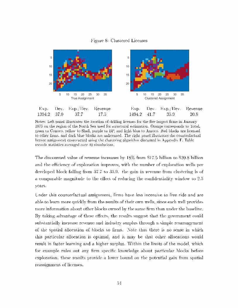
Figure 8: Clustered Licenses

Exp. Dev. Exp./Dev. Revenue Exp. Dev. Exp./Dev. Revenue1394.2 37.0 37.7 17.5 1494.2 41.7 35.9 20.8

Notes: Left panel illustrates the location of drilling licenses for the ve largest rms in January1975 on the region of the North Sea used for structural estimation. Orange corresponds to Total,green to Conoco, yellow to Shell, purple to BP, and light blue to Amoco. Red blocks are licensedto other rms, and dark blue blocks are unlicensed. The right panel illustrates the counterfactuallicense assignment constructed using the clustering algorithm discussed in Appendix F. Tablerecords statistics averaged over 40 simulations.

The discounted value of revenue increases by 18% from $17.5 billion to $20.8 billion

and the eciency of exploration improves, with the number of exploration wells per

developed block falling from 37.7 to 35.9. the gain in revenue from clustering is of

a comparable magnitude to the eect of reducing the condentiality window to 2.5

years.

Under this counterfactual assignment, rms have less incentive to free ride and are

able to learn more quickly from the results of their own wells, since each well provides

more information about other blocks owned by the same rm than under the baseline.

By taking advantage of these eects, the results suggest that the government could

substantially increase revenue and industry surplus through a simple rearrangement

of the spatial allocation of blocks to rms. Note that there is no sense in which

this particular allocation is optimal, and it may be that other allocations would

result in faster learning and a higher surplus. Within the limits of the model, which

for example rules out any rm specic knowledge about particular blocks before

exploration, these results provide a lower bound on the potential gain from spatial

reassignment of licenses.

54

As with the condentiality window, it is worth asking why the actual allocation of

licenses to rms does not appear to fully take into account information externalities.

The allocation mechanism that has been in place since the rst licenses were issued in

1964 has relied on rms submitting applications for specic blocks. One reason that

rms may not apply for a large number of licenses close together is that this type of

clustered allocation increases the risk borne by each individual rm. Because of the

spatial correlation of oil deposits, a risk averse rm with a constant prior mean would

prefer to be allocated licenses that are spread over a wide area. Under risk aversion,

clustered license allocations are therefore likely to be industry-optimal but not optimal

in expectation for the individual rms. Application data is condential, so I cannot

empirically verify whether rms' applications are spatially dispersed. However, in

my conversations with the regulator I learned that the government has occasionally

recommended rms take on licenses for blocks for which they did not apply in order to

create contiguous blocks of licenses like those generated by the clustering algorithm.

One alternative policy that could achieve some of the gain from license clustering

would be to require rms to apply for licenses at a regional rather than block level,

with the government determining the exact allocation of blocks to rms within the

region.

9 Conclusion

In many industries the creation of new knowledge through R&D is carried out in a

decentralized manner by competing rms. The growth of the industry-wide stock

of knowledge depends on the extent to which rms can observe and build on each

other's innovations. Allowing information spillovers between rms can improve the

speed of cumulative research and reduce duplicative or socially inecient investments.

On the other hand, information spillovers can diminish rms' individual incentives

to innovate by enabling free riding on the innovations of other rms. The design of

property rights over innovations plays an important role in balancing these eects.

I study the eects of information spillovers on R&D in the context of oil exploration,

using historical data from the UK North Sea. Oil exploration by individual rms can

be thought of as a process of cumulative learning about the location of oil deposits.

Exploration wells are experiments located in geographical space with observable out-

55

comes. If rms can learn from the results of other rms' wells they face an incentive

to delay exploration. However, if other rms' well outcomes are unobserved rms

are likely to make inecient drilling decisions, for example exploring regions that are

known by other rms to be unproductive.

To quantify the eects of information spillovers, I build and estimate a model of the

rm's dynamic exploration problem with spatial learning and information spillovers

across rms. The estimated model indicates that there is imperfect information ow

between rms. In counterfactual simulations, I show that removing the incentive to

free ride brings exploration and development forward in time, increasing the number

of exploration wells drilled between 1965 and 1990 by 17.6% and increasing indus-

try surplus in the same time period by 27%. Holding the free riding incentive xed

and allowing perfect information ow between rms increases surplus by 5.4% by

increasing the speed of learning, increasing the cost eciency of exploration by re-

ducing the number of development wells drilled per developed block, and increasing

the concentration of development on productive blocks.

Equilibrium simulations under counterfactual property rights policies highlight the

tradeo between free riding and ecient cumulative research. Strengthening property

rights by extending the well data condentiality period increases industry surplus by

increasing the rate of exploration, while weakening property rights by limiting the

condentiality period increases industry surplus by increasing the speed of learning

and eciency of exploration. Over the range of policies I examine, reducing the

condentiality window to 2.5 years achieves the highest industry surplus.

Notice that the gains from strengthening property rights here are due to the eect

of limiting inter-rm information ow on the incentive to free ride on other rms'

discoveries. This diers from the more commonly discussed motive of allowing rms

to capture the surplus from their innovations. In this setting, the ability of rms to

prot from their discoveries is held xed across alternative policies. Firms always

have the right to extract the oil they nd on their blocks, with only the ability to

benet from other rms' investments changing across alternative policies. The specic

features of this setting mean that the information externality eects of variation in

property rights are not conated with changes in the ability of a rm to prot from

its own discoveries.

There is a substantial body of recent work quantifying the extent to which property

56

rights limit follow-on research in a number of settings (Murray and Stern, 2007;

Williams, 2013; Murray et al., 2016), but little empirical work on the potential for

weaker property rights to encourage free riding. The policy results in this paper

suggest that the question of the optimal generosity of property rights is subtle, even

in the absence of an eect of stronger property rights on rms' ability to extract rent

from their discoveries. In some settings it may be optimal to strengthen property

rights to reduce the free riding incentive even though stronger property rights hinder

cumulative research.

The nal set of results quanties the eect of changing the spatial allocation of licenses

to rms. By clustering licenses, the regulator is able to reduce the incentive to free ride

and increase the speed of learning, since each rm learns more about its own blocks

from a single well. The eects of clustering on industry surplus are large, increasing

surplus by more than the no free riding counterfactual. This nding is related to

the theoretical literature on learning in teams (Holmstrom, 1982; Campbell, Ederer,

and Spinnewijn, 2013), and suggests in settings where research is decentralized but

a social planner is able to assign projects to each researcher (here, oil rms), surplus

can be enhanced by designing the assignment to minimize the extent to which each

team member can free ride o the others' research and maximize the extent to which

each team member's research is cumulative. This insight could, for example, have

applications to the organization of publicly funded research eorts which involve

many independent researchers and labs contributing to a common project.

Methodologically, this paper makes two contributions that are applicable to other

settings. First, the model of beliefs and learning can be used to study other indus-

tries where research takes place in a well dened space. For example, measures of

molecular similarity are important metrics in the exploratory phase of pharmaceu-

tical development, and measures of the distance between molecular structures are

increasingly used in the economics literature on pharmaceutical R&D (Krieger, Li,

and Papanikolau, 2017; Cunningham, Ederer, and Ma, 2018). An application of this

model to research in chemical space might be able to inform the design of property

rights, for example the disclosure of clinical trial results, in that industry. Second,

the estimation approach developed in this paper is potentially applicable to other

settings in which agents have asymmetric information and the econometrician is not

fully informed about each agent's information set.

57

References

Agerton, M. 2018. Learning Where to Drill: Drilling Decisions and Geological Qual-

ity in the Haynesville Shale. Working Paper.

Agarwal, N. and P. Somaini. 2018. Demand Analysis Using Strategic Reports: An

Application to a School Choice Mechanism. Econometrica. 86 (2) 391-444.

Ali, S. N., A. Chen-Zion, and E. Lillethun. 2017. Reselling Information. Working

Paper.

Anton, J. J., and D. A. Yao. 2002. The Sale of Ideas: Strategic Disclosure, Property

Rights, and Contracting. Review of Economic Studies. 69, 513-531.

Arcidiacono, P., and R. A. Miller. 2011. Conditional Choice Probability Estimation

of Dynamic Discrete Choice Models with Unobserved Heterogeneity. Economet-

rica. 79 (6), 1823-1867.

Arrow, K. J. 1971. Economic Welfare and the Allocation of Resources for Invention.

in Essays in the Theory of Risk Bearing. Chicago: Markham.

Bajari, P., C. L. Benkard, and J. Levin. 2007. Estimating Dynamic Models of

Imperfect Competition. Econometrica. 75 (5), 1331-1370.

Berry, S. and G. Compiani. 2021. Empirical Models of Industry Dynamics with

Endogenous Market Structure. Annual Review of Economics. 13 11.1-11.26.

Bessen, J. 2004. Holdup and Licensing of Cumulative Innovations with Private

Information. Economics Letters. 82 (3), 321-326.

Bickel, J. E., and J. E. Smith. 2006. Optimal Sequential Exploration: A Binary

Learning Model. Decision Analysis. 3 (1), 1-59.

Bolton, P., and C. Harris. 1999. Strategic Experimentation. Econometrica. 67 (2),

349-174.

Bolton, P., and J. Farrell. 1990. Decentralization, Duplication, and Delay. Journal

of Political Economy. 98 (4), 803-826.

Brennand, T. P., B. Van Hoorn, K. H. James, and K. W. Glennie. 1998. Historical

Review of North Sea Exploration. in Petroleum Geology of the North Sea.

Oxford: Blackwell.

58

Campbell, A., F. Ederer, and J. Spinnewijn. 2013. Delay and Deadlines: Freerid-

ing and Information Revelation in Partnerships. American Economic Journal:

Microeconomics. 6 (2), 163-204.

Collard-Wexler, A. 2013. Demand Fluctuations in the Ready-Mix Concrete Indus-

try. Econometrica. 81 (3), 1003-1037.

Covert, T. R. 2015. Experimental and Social Learning in Firms: The Case of Hy-

draulic Fracturing in the Bakken Shale. Working Paper.

Cressie, N. 1991. Statistics for Spatial Data. New York: Wiley.

Cunningham, C., F. Ederer, and S. Ma. 2018. Killer Acquisitions. Working Paper.

Dasgupta, P., and J. Stiglitz. 1977. Industrial Structure and the Nature of Innovative

Activity. Economic Journal. 90 (358), 266-293.

Diggle, P. J., J. A. Tawn, and R. A. Moyeed. 1998. Model-based Geostatistics.

Applied Statistics. 47 (3) 299-350.

Dong, M. 2018. Strategic Experimentation with Asymmetric Information. Working

Paper.

Doraszelski, U, Lewis, G., and A. Pakes. 2018. Just Starting Out: Learning and

Equilibrium in a New Market. American Economic Review. 108 (3) 565-615.

Farrell, J. 1987. Information and the Coase Theorem. Journal of Economic Per-

spectives. 1 (2) 113-129.

Fershtman., C. and A. Pakes. 2012. Dynamic Games with Asymmetric Information:

A Framework for Empirical Work. Quarterly Journal of Economics 127 (4)

1611-1661.

Gordon, G. W. 2015. Production Licensing on UK Continental Shelf: Ministerial

Powers and Controls. LSU Journal of Energy Law and Resources. 4 (1), 75-95.

Gourieroux, C., and A. Monfort. 1993. Simulation-Based Inference. Journal of

Econometrics. 59, 5-33.

Haile, P., K. Hendricks, and R. H. Porter. 2010. Recent U.S. Oshore Oil and

Gas Lease Bidding: A Progress Report. International Journal of Industrial

Organization. 28 (4), 390-396.

59

Hendricks, K., and D. Kovenock. 1989. Asymmetric Information, Information Ex-

ternalities, and Eciency: The Case of Oil Exploration. RAND Journal of

Economics. 20 (2), 164-182.

Hendricks, K. and R. H. Porter. 1996. The Timing and Incidence of Exploratory

Drilling on Oshore Wildcat Tracts. American Economic Review. 86 (3), 388-

407.

Hohn, M. E. 1999. Geostatistics and Petroleum Geology. Dordrecht: Kluwer Aca-

demic Publishers.

Holmstrom, B. 1982. Moral Hazard in Teams. The Bell Journal of Economics. 13

(2), 324-340.

Hotz, V. J., and R. A. Miller. 1993. Conditional Choice Probabilities and the

Estimation of Dynamic Models. The Review of Economic Studies. 60 (3), 497-

529.

Hotz, V. J., R. A. Miller, S. Sanders, and J. Smith. 1994. A Simulation Estimator

for Dynamic Models of Discrete Choice. The Review of Economic Studies. 61

(2) 265-289.

Hunter, T. 2015. Regulation of the Upstream Petroleum Sector. Cheltenham:

Edward Elgar.

Jae, A, M. Trajtenberg, and R. Henderson. 1993. Geographic Localization of

Knowledge Spillovers as Evidenced by Patent Citations. Quarterly Journal of

Economics. 113 (4), 1137-1167.

Jahn, F., M. Cook, and M. Graham. 1998. Hydrocarbon Exploration and Produc-

tion. Amsterdam: Elsevier.

Kasahara, H., and K. Shimotsu. 2008. Nonparametric Identication of Finite Mix-

ture Models of Dynamic Discrete Choices. Econometrica. 77 (1) 135-175.

Kellogg, R. 2011. Learning by Drilling: Interrm Learning and Relationship Persis-

tence in the Texas Oilpatch. Quarterly Journal of Economics. 126 (4), 1961-

2004.

Kemp, A. 2012a. The Ocial History of North Sea Oil and Gas Vol. I: The Growing

Dominance of the State. New York: Routledge.

60

Kemp, A. 2012b. The Ocial History of North Sea Oil and Gas: Vol. II: Moderating

the State's Role. New York: Routledge .

Krieger, J., D. Li, and D. Papanikolaou. 2017. Developing Novel Drugs. Working

Paper.

Kullback, S. 1997. Information Theory and Statistics. New York: Dover.

Laont, J. J., H. Ossard, and Q. Vuong. 1995. Econometrics of First-Price Auctions.

Econometrica. 63 (4), 953-980.

Lerche, I, and J. A. MacKay. 1995. Economic Risk in Hydrocarbon Exploration.

San Diego: Academic Press.

Levitt, C. J. 2009. Learning Through Oil and Gas Exploration. Working Paper.

Levitt, C. J. 2016. Information Spillovers in Onshore Oil and Gas Exploration.

Resource and Energy Economics. 45, 80-98.

Lin, C.-Y. C, 2009. Estimating Strategic Interactions in Petroleum Exploration.

Energy Economics. 31 (4), 586-594.

Lin, C.-Y. C., 2013. Strategic Decision Making with Information Externalities: A

Structural Model of the Multistage Investment Game in Oshore Petroleum Pro-

duction. The Review of Economics and Statistics. 95 (5), 1601-1621.

MacKay, D. J. C. 2003. Information Theory, Inference, and Learning Algorithms.

Cambridge: Cambridge University Press.

Mardia, K. V., and R. J. Marshall. 1984. Maximum Likelihood Estimation of Models

for Residual Covariance in Spatial Regression. Biometrika. 71 (1), 135-146.

Murray, F., P. Aghion, M. Dewatripont, J. Kolev, and S. Stern. 2016 Of Mice

and Academics: Examining the Eect of Openness on Innovation. American

Economic Journal: Economic Policy. 8 (1) 212-252.

Murray, F. and S. Stern. 2007. Do Formal Intellectual Property Rights Hinder the

Free Flow of Scientic Knowledge? An Empirical Test of the Anti-commons

Hypothesis. Journal of Economic Behavior and Organization. 63 (4), 648-687.

Moreton, R. 1995. Tales from Early UK Oil Exploration: 1960-1979. Croydon:

Petroleum Exploration Society of Great Britain.

Myerson, R. B, and M. A. Satterthwaite. 1981. Ecient Mechanisms for Bilateral

Trading. Journal of Economic Theory. 29, 265-281.

61

Porter, R. H. 1995 The Role of Information in U.S. Oshore Oil and Gas Lease

Auctions. Econometrica. 63 (1). 1-27.

Rasmussen, C. E., and C. K. I. Williams. 2005. Gaussian Processes for Machine

Learning. Cambridge: The MIT Press.

Rowland, C., and D. Hann. 1987. The Economics of North Sea Oil Taxation.

London: Palgrave Macmillan.

Ryan, S. P., and C. Tucker. 2011. Heterogeneity and the Dynamics of Technology

Adoption. Quantitative Marketing and Economics. 10, 63-103.

Scotchmer, S. 1991. Standing on the Shoulders of Giants: Cumulative Research and

the Patent Law. Journal of Economic Perspectives. 5 (1), 29-41.

Spence, M. 1984. Cost Reduction, Competition, and Industry Performance. Econo-

metrica. 52 (1), 101-122.

Steck, A. 2018. Industry Dynamics with Social Learning: Evidence from Hydraulic

Fracturing. Working Paper.

Williams, H. 2013. Intellectual Property Rights and Innovation: Evidence from the

Human Genome. Journal of Political Economy. 121 (1), 1-27.

62

Appendix

A Theoretical Framework

In this section, I present a simple model of exploration to illustrate the eects of

information externalities on rms' drilling decisions and structure the subsequent

empirical analysis. Consider a two period drilling game played by two rms, i and j,

who control adjacent blocks. In the rst period, rms simultaneously decide whether

to drill an exploration well on their respective blocks. Exploration wells on block i

provide a binary signal about the presence of oil, and are successful with probability

ρi ∈ (0, 1), which is a primitive determined by technology and the geology of the region

being explored. Each rm always observes whether their own well is successful, and

observes whether or not a well drilled by the rival rm is successful with probability

α ∈ [0, 1]. In the second period, rms decide whether or not to develop the block at

cost κ. Development yields a payo π(ρi) > 0 with π′(ρi) > 0, π(0) < κ, and π(1) > κ,

which can be thought of as the expected present discounted prot from the ow of

oil over the block's lifetime. In reality, although exploration wells yield more complex

geological data, the success rate of wells based on a binary wet/dry classication is an

important statistic in determining whether to develop, continue exploring, or abandon

a block. See for example Lerche and MacKay (1995) and Bickel and Smith (2006) who

present models of optimal sequential exploration decisions based on binary signals.

Firm i's decision in each period depends on their beliefs about ρi ∈ [0, 1], the proba-

bility of exploration well success on their block. Suppose that rms have a common

prior belief that the vector ρ = (ρi, ρj) is drawn from a distribution F (ρ). Let σij

be the correlation between ρi and ρj implied by F (ρ). Let Iit = (ownit, otherit) be

rm i's information at the beginning of period t. ownit ∈ −1, 0, 1 records rm i's

exploration well outcomes from period t− 1. If ownit = 1, rm i drilled a successful

exploration well, if ownit = −1, rm i drilled an unsuccessful well, and if ownit = 0,

rm i did not drill an exploration well. otherit ∈ −1, 0, 1 is rm i's information

about rm j's exploration well outcomes, dened analogously except that otherit = 0

if rm j drilled a well and rm i did not observe it. Let G(ρ|I) be the Bayesian pos-

terior distribution of ρ given observed outcomes I. Assume Ii1 = (0, 0) and therefore

G(ρ|Ii1) = F (ρ) for both rms. Firms start period 1 with identical information and

63

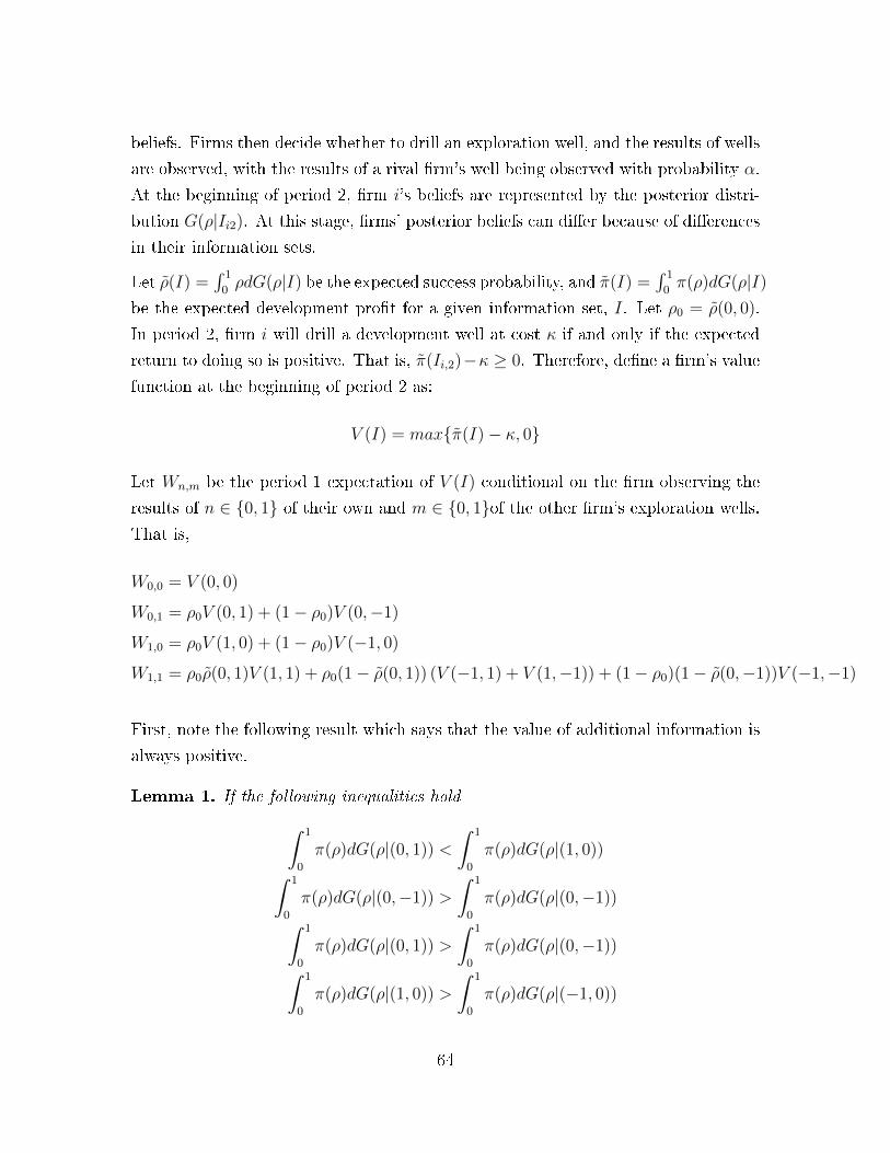
beliefs. Firms then decide whether to drill an exploration well, and the results of wells

are observed, with the results of a rival rm's well being observed with probability α.

At the beginning of period 2, rm i's beliefs are represented by the posterior distri-

bution G(ρ|Ii2). At this stage, rms' posterior beliefs can dier because of dierences

in their information sets.

Let ρ(I) =∫ 1

0ρdG(ρ|I) be the expected success probability, and π(I) =

∫ 1

0π(ρ)dG(ρ|I)

be the expected development prot for a given information set, I. Let ρ0 = ρ(0, 0).

In period 2, rm i will drill a development well at cost κ if and only if the expected

return to doing so is positive. That is, π(Ii,2)−κ ≥ 0. Therefore, dene a rm's value

function at the beginning of period 2 as:

V (I) = maxπ(I)− κ, 0

Let Wn,m be the period 1 expectation of V (I) conditional on the rm observing the

results of n ∈ 0, 1 of their own and m ∈ 0, 1of the other rm's exploration wells.

That is,

W0,0 = V (0, 0)

W0,1 = ρ0V (0, 1) + (1− ρ0)V (0,−1)

W1,0 = ρ0V (1, 0) + (1− ρ0)V (−1, 0)

W1,1 = ρ0ρ(0, 1)V (1, 1) + ρ0(1− ρ(0, 1)) (V (−1, 1) + V (1,−1)) + (1− ρ0)(1− ρ(0,−1))V (−1,−1)

First, note the following result which says that the value of additional information is

always positive.

Lemma 1. If the following inequalities hold∫ 1

0

π(ρ)dG(ρ|(0, 1)) <

∫ 1

0

π(ρ)dG(ρ|(1, 0))∫ 1

0

π(ρ)dG(ρ|(0,−1)) >

∫ 1

0

π(ρ)dG(ρ|(0,−1))∫ 1

0

π(ρ)dG(ρ|(0, 1)) >

∫ 1

0

π(ρ)dG(ρ|(0,−1))∫ 1

0

π(ρ)dG(ρ|(1, 0)) >

∫ 1

0

π(ρ)dG(ρ|(−1, 0))

64

then W1,1 ≥ W1,0 ≥ W0,1 ≥ W0,0.

Proof. Suppose∫ 1

0π(ρ)dF (ρ)− κ > 0, so W0,0 =

∫ 1

0π(ρ)dF (ρ)− κ. Note that∫ 1

0

π(ρ)dF (ρ)− κ =

∫ 1

0

π(ρ)dG(ρ|(0, 1))ρ0 +

∫ 1

0

π(ρ)dG(ρ|(0,−1))(1− ρ0)− κ

≤ ρ0V (0, 1) + (1− ρ0)V (0,−1).

Now suppose∫ 1

0π(ρ)dF (ρ)−κ ≤ 0, so W0,0 = 0. It cannot be the case that W0,1 < 0,

so in either case, W0,1 ≥ W0,0. Similar arguments can be used to show W1,0 ≥ W0,0,

W1,1 ≥ W0,0, W1,1 ≥ W0,1, and W1,1 ≥ W1,0.

It remains to be shown thatW1,0 ≥ W0,1. Assume by way of contradiction thatW1,0 <

W0,1. It must be the case that either∫ 1

0π(ρ)dG(ρ|(1, 0))−κ < 0 or

∫ 1

0π(ρ)dG(ρ|(−1, 0))−

κ < 0.

In the rst case,∫ 1

0π(ρ)dG(ρ|(−1, 0))−κ < 0, soW1,0 = 0, and

∫ 1

0π(ρ)dG(ρ|(0,−1)) <∫ 1

0π(ρ)dG(ρ|(0, 1)) < 0, so W0,1 = 0, a contradiction.

In the second case, it must be that∫ 1

0π(ρ)dG(ρ|(1, 0)) − κ > 0, otherwiseW1,0 =

W0,1 = 0, a contradiction. It must also be that∫ 1

0π(ρ)dG(ρ|(0,−1))−κ > 0, otherwise

W1,0 > W0,1, a contradiction. Thus,

W1,0−W0,1 =

∫ 1

0

π(ρ)dG(ρ|(1, 0))ρ0−∫ 1

0

π(ρ)dG(ρ|(0, 1))ρ0−∫ 1

0

π(ρ)dG(ρ|(0,−1))(1−ρ0).

Note that since the following two equalities hold∫ 1

0

π(ρ)dF (ρ)− κ =

∫ 1

0

π(ρ)dG(ρ|(0, 1))ρ0 +

∫ 1

0

π(ρ)dG(ρ|(0,−1))(1− ρ0)− κ∫ 1

0

π(ρ)dF (ρ)− κ =

∫ 1

0

π(ρ)dG(ρ|(1, 0))ρ0 +

∫ 1

0

π(ρ)dG(ρ|(−1, 0))(1− ρ0)− κ

it must be the case that

ρ0

∫ 1

0

π(ρ)dG(ρ|(1, 0))− ρ0∫ 1

0

π(ρ)dG(ρ|(0, 1))

= (1− ρ0)(∫ 1

0

π(ρ)dG(ρ|(0,−1))−∫ 1

0

π(ρ)dG(ρ|(−1, 0))

)65

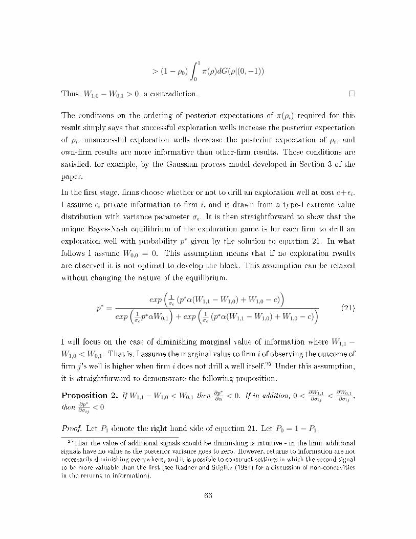
> (1− ρ0)∫ 1

0

π(ρ)dG(ρ|(0,−1))

Thus, W1,0 −W0,1 > 0, a contradiction.

The conditions on the ordering of posterior expectations of π(ρi) required for this

result simply says that successful exploration wells increase the posterior expectation

of ρi, unsuccessful exploration wells decrease the posterior expectation of ρi, and

own-rm results are more informative than other-rm results. These conditions are

satised, for example, by the Gaussian process model developed in Section 3 of the

paper.

In the rst stage, rms choose whether or not to drill an exploration well at cost c+εi.

I assume εi private information to rm i, and is drawn from a type-I extreme value

distribution with variance parameter σε. It is then straightforward to show that the

unique Bayes-Nash equilibrium of the exploration game is for each rm to drill an

exploration well with probability p∗ given by the solution to equation 21. In what

follows I assume W0,0 = 0. This assumption means that if no exploration results

are observed it is not optimal to develop the block. This assumption can be relaxed

without changing the nature of the equilibrium.

p∗ =exp

(1σε

(p∗α(W1,1 −W1,0) +W1,0 − c))

exp(

1σεp∗αW0,1

)+ exp

(1σε

(p∗α(W1,1 −W1,0) +W1,0 − c)) (21)

I will focus on the case of diminishing marginal value of information where W1,1 −W1,0 < W0,1. That is, I assume the marginal value to rm i of observing the outcome of

rm j's well is higher when rm i does not drill a well itself.25 Under this assumption,

it is straightforward to demonstrate the following proposition.

Proposition 2. If W1,1 −W1,0 < W0,1 then ∂p∗

∂α < 0. If in addition, 0 <∂W1,1

∂σij<

∂W0,1

∂σij,

then ∂p∗

∂σij< 0

Proof. Let P1 denote the right hand side of equation 21. Let P0 = 1− P1.

25That the value of additional signals should be diminishing is intuitive - in the limit additionalsignals have no value as the posterior variance goes to zero. However, returns to information are notnecessarily diminishing everywhere, and it is possible to construct settings in which the second signalto be more valuable than the rst (see Radner and Stiglitz (1984) for a discussion of non-concavitiesin the returns to information).

66

Applying the implicit function theorem to equation 21 yields

∂p∗

∂α= −

(p∗P1P0 (W11 −W10 −W01)

αP1P0 (W11 −W10 −W01)− σε

),

which is < 0 if W1,1 −W1,0 < W0,1.

Applying the same approach to obtain the derivative with respect to σij, noting that∂W0,1

∂σij6= 0, ∂W1,1

∂σij6= 0, and ∂W1,0

∂σij= 0, yields

∂p∗

∂σij= −

p∗P1P0

(∂W1,1

∂σij− ∂W0,1

∂σij

)αP1P0 (W11 −W10 −W01)− σε

,

which is < 0 if W1,1 −W1,0 < W0,1 and 0 < ∂W1,1

∂σij< ∂W0,1

∂σij.

The rst part of this theorem says that as the probability of information spillover

between rms increases, the equilibrium exploration probability falls. If rms are more

likely to observe the results of their rival's exploration wells, then rms have more of

an incentive to free ride since the relative expected value of drilling their own well falls.

The second part of this theorem says that the equilibrium probability of exploration

is negatively related to the correlation between ρi and ρj, as long as 0 < ∂W1,1

∂σij<

∂W0,1

∂σij. This property applies, for example, if ρi and ρj are distributed according to

a transformation of a multivariate Niormal distribution, as in the Gaussian process

model developed in Section 3 of the paper. Intuitively, increased correlation between

rms' signals has a larger eect of a rm's continuation value when they only observe

the other rm's signal and not their own. There is more incentive for rms to free

ride when the signals generated by exploration wells on dierent blocks are more

correlated. In particular, if ρi = ρj (perfect correlation) then information generated

by rm j's exploration well is of equal value to rm i as information generated by

its own exploration well. In this case, W1,0 = W0,1. If there is no correlation, then

signals generated by rm j are not informative about ρi, and W1,1 = W1,0 and W0,1 =

0. In this case, the equilibrium exploration rate, p∗, is identical to the equilibrium

exploration rate that obtains when α = 0.

This result illustrates that the extent to which rms have an incentive to free ride

in exploration depends on the information ow between rms - parameterized by

67

α - and the covariance of signals generated by exploration wells on dierent blocks

- parameterized by σij. Information ow is largely a function of technology and

regulation - for example, the information condentiality period imposed by the UK

regulator. Correlation of exploration well outcomes at dierent locations is a function

of underlying geology and the size and arrangement of license blocks. The remainder

of this paper uses the UK data to estimate empirical analogues of these objects

in the context of North Sea oil exploration and quanties the eect of information

externalities on industry surplus using an econometric model that builds on the simple

theoretical model presented here.

A nal theoretical result illustrates the trade o faced by the social planner in ma-

nipulating information ow between rms.

Proposition 3. Let p be the probability of exploration that maximizes the joint ex-

pected surplus of the two rms. Let p be the equilibrium probability when α = 0, and p

be the equilibrium probability when α = 1. If W10 > c and W1,0+W0,1−c > 2W1,1−2c,

then for some value of σε, p < p < p.

Proof. First, note that ifW1,0 > c, then p→ 1 and p→ 1 as σε →∞ and p→ 0.5 and

p→ 0.5 as σε → 0. Note also that p > p for any value of σε ∈ (0,∞) by Proposition

1. Since equation 21 is continuous in σε, for any p ∈ (0.5, 1) there exists a value

σε ∈ (0,∞) such that p > p > p.

Now, write the objective function of the planner who can set the probability of ex-

ploration and observes all well outcomes as:

p = arg maxp∈[0,1]

p2(2W1,1 − 2c) + 2p(1− p)(W1,0 +W0,1 − c).

The planner's optimum is given by:

p =1

2

(W1,0 −W0,1 − c

W1,0 +W0,1 −W1,1

).

If W1,0 > c, then W1,1 > c and therefore p > 0.5. furthermore, if W1,0 + W0,1 − c >2W1,1 − 2c then p < 1.

The condition W10 > c says that the social planner would prefer to drill a well on one

of the blocks than none of the blocks. The condition W1,0 + W0,1 − c > 2W1,1 − 2c

68

holds when the value of information is suciently concave such that the social planner

would like to drill only one well on one of the blocks. This result shows that the

decentralized equilibrium can generate either too many or too few wells in expectation,

and information ow between rms can be too high or too low. Values of α that

are too close to one induce too much free riding, such that the expected number of

exploration wells is too low. On the other hand, low values of α make is more likely

that more than one exploration well is drilled. This result illustrates the countervailing

eects of information ow between rms on social surplus in equilibrium. Too little

information ow results in socially inecient exploration, since the social value of

additional exploration wells beyond the rst is lower than c. On the other hand, too

much information ow between rms increases the free riding incentive and results in

too little exploration in equilibrium.

This result suggests that exploration behavior is a decentralized equilibrium may be

suboptimal, and that government policy that manipulates the arrangement of licenses

(and thus the correlation of signals between rms) or the information ow between

rms might bring equilibrium exploration rates closer to the social optimum.

B Details of Logistic Gaussian Process Model

This section describes the Bayesian updating rule for the logistic Gaussian process

model and relies heavily on Section 3 of Rasmussen and Williams (2006). The code

that I use to implement the numerical Bayesian updating rule is a modied version

of the Matlab package made available by Rasmussen and Williams.26

The latent variable, λ(X) is assumed to be distributed according at a Gaussian pro-

cess. That is, λ(X) is a continuous function, and any nite collection of K locations

1, ..., K, the vector (λ(X1), ..., λ(XK)) is a multivariate normal random variable

with mean (µ(X1), ..., µ(XK)) and a covariance matrix with (j, k) element κ(Xj, Xk)

where κ(Xj, Xk)→ κ(Xj, Xj) as |Xj −Xk| → 0.

I assume a constant prior mean and a covariance specication given by equation 2.

The prior distribution is therefore dened by three parameters, (µ, ω, `). Denote the

density function of prior distribution of λ by p0(λ). Observed data is described by

26Available at http://www.gaussianprocess.org/.

69

y = (s(w), Xw)w∈W for a set of wells, W . The Bayesian posterior distribution of λ

conditional on y is given by:

p1(λ|y) =p0(λ)p(y|λ)

p(y)(22)

p(y|λ) =∏w∈W

(1(s(w) = 1)ρ(λ(Xw)) + 1(s(w) = 0) (1− ρ(λ(Xw))))

p(y) =∏w∈W

(1(s(w) = 1)

∫ρ(λ(Xw))p0(λ)dλ+ 1(s(w) = 0)

(1−

∫ρ(λ(Xw))p0(λ)dλ

))

Where ρ(λ(X)) is dened by equation 1. This posterior distribution is dicult to

work with. In particular, in order to compute the posterior E(ρ(X)|y) for some

location X I must rst compute the marginal distribution of λ(X), which is given by:

p(λ(X) = λ|y) =

∫1(λ(X) = λ)p1(λ|y)dλ (23)

Then the expected value of ρ(X) is given by:

E(ρ(X)|y) =

∫ρ(λ)p(λ(X) = λ|y)dλ (24)

The posterior marginal distribution of λ(X) given by equation 23 is non-gaussian and

has no analytical expression. This means that it is computationally costly to compute

E(ρ(X)|y).

To solve this problem I use a Gaussian approximation to the posterior p1(λ|y) com-

puted using the Laplace approximation technique detailed in Section 3.4 of Rasmussen

and Williams (2006), based on Willaims and Barber (1998). This method is widely

used for Bayesian classication problems in computer science and in geostatistics

(Diggle, Tawn, and Moyeed, 1998)..

Denote the Gaussian approximation to p1(λ|y) by q1(λ|y). Since q1(λ|y) is Gaussian,

the posterior distribution over any nite collection of K locations can be written as a

N(µ1,Σ1) where µ1 is K×1 and Σ1 is K×K. In particular, the marginal distribution

given by equation 23 is a Normal distribution.

Notice that, since q1(λ|y) is itself a Gaussian process, it is straightforward to update

beliefs again given a new set of data, y′, following the same procedure. This updating

70

procedure denes the operator B(·) in equation 4, where G(ρ) is the distribution of

ρ implied by the prior Gaussian distribution of λ and the logistic squashing function

1, and G′(ρ) is the distribution over ρ dened by the Gaussian approximation to the

posterior distribution of λ.

B.1 KL Divergence

I compute the expected KL divergence for each (j, t) according to the following equa-

tion:

KLjt = Et(ρj)

∫gt(ρ|j, 1) log

(gt(ρ|j, 1)

gt(ρ)

)dρ

+ (1− Et(ρj))∫gt(ρ|j, 0) log

(gt(ρ|j, 0)

gt(ρ)

)dρ (25)

Where gt(ρ) is the density of the rm's posterior beliefs over the vector ρ after ob-

serving all wells up to date t, gt(ρ|j, 1) is the updated posterior after observing an

additional successful well on block j, and gt(ρ|j, 0) is the updated posterior after

observing an additional unsuccessful well on block j. The rst term in the expression

is the expected probability of success on block j multiplied by the information gain

from a successful well on that block. The second term is the expected probability of

failure on block j multiplied by the information gain from a failed well.

C Estimation Details

C.1 Estimating Conditional Choice Probabilities

In the rst step, I estimate CCPs P (aE = j|S) and P (aD = j|S) - the probabilities

that a rm takes an action j in the exploration and development stages of the game

conditional on its state S. With a suciently large data set, these probabilities could

be estimated as empirical means for each state. However, since the number of possible

states is large relative to the data, I impose some additional structure. Consider rst

71

the exploration decision. Notice that equation 10 can be rewritten as

P (aEf = j|S) =exp

(vEf (j,S)

)1 +

∑k∈Jft exp

(vEf (k,S))

) (26)

where vEf (j,S) = 1σεvEf (j,S)− 1

σεvEf (0,S).

I approximate vfE(j,S) with a linear equation with the following terms:

A cubic function of the mean and variance of the rm's beliefs: E(ρj|Gft),

V ar(ρj|Gft).

An indicator for whether rm f has observed any past well outcome on block

j.

The number of licenses held near block j by rm f and by other rms: |k :

k ∈ Jft and d(j, k) ≤ 3|, |k : k ∈ ∪Jgtg 6=f and d(j, k) ≤ 3|, and |k :

k ∈ ∪Jgtg 6=f and d(j, k) = 0|, where d(j, k) = 1 if j and k are neighbors,

d(j, k) = 2 if j and k are second degree neighbors etc.

The number of rms operating near block j: |g : ∃k ∈ Jgt : d(j, k) ≤ 3|.

A quadratic in the price level: Pt and P2t .

Interactions of Pt with E(ρj|Gft) and V ar(ρj|Gft).

The approximation to vfD(j,S) is contains fewer terms because of the limited number

of development actions observed in the data.

Estimating P (aEf = j|S) is then a case of estimating the parameters of this approx-

imation to vfE(j,S). Notice that the approximation to vf

E(j,S) depends on the

distribution of licenses and beliefs near block j, rather than on the entire set of li-

censes ∪Jgt and the entire distribution Gft. Intuitively, the dierence between the

value of drilling on block j and taking no action should not depend on the distribution

of licenses and wells at distant locations

If the state variable were observable in the data, then P (aEf = j|S) could be estimated

using the likelihood function implied by equation 26. However, the asymmetric in-

formation structure of the model means that the true state is not observed by the

72

econometrician. The data does not include the vector of that records which other-rm

well outcomes were observed by rm f . Dierent realizations of of imply dierent

states through the eect of observed well outcomes on Gft. The data is therefore

consistent with a set of possible states Sf for each rm.27

To recover CCP estimates, observe that dierent values of the parameter α dene

distributions P (Sf |Sf , α) over the elements of Sf . For example, suppose at date t

there was one other-rm well w that may have been observed by rm f . Let S1ft be

the state if of (w) = 1 and S0ft be the state if of (w) = 0. From the econometrician's

perspective, P (S1ft|S1

ft,S0ft, α) = α. I provide a formal denition of the distribution

P (Sf |Sf , α) in subsection C.4 below.

Given this distribution over states, the likelihood of a sequence of exploration choice

observations is:

LEf =∑Sf∈Sf

T∏t=1

∏j∈Jft∪0

P (aEft = j|S)1(aEft=j)P (aDft = j|S)1(a

Dft=j)

P (Sf |Sf , α)

.(27)

I maximize this likelihood to jointly estimate the coecients of the approximations

vEf (j,Sft) and vDf (j,Sft), and the parameter α. Since I sometimes observe multiple

exploration wells for the same (f, t) I treat these as separate observations inside the

brackets in equation 27. The estimated coecients imply conditional choice proba-

bility estimates, P (aE = j|S) and P (aD = j|S).

Logit coecients for the estimated CCPs are recorded in Table A1.

27More precisely, and element of Sf is a particular sequence of rm-f states Sf = SftTt=1. See

the subsection below for a formal denition of Sf .

73

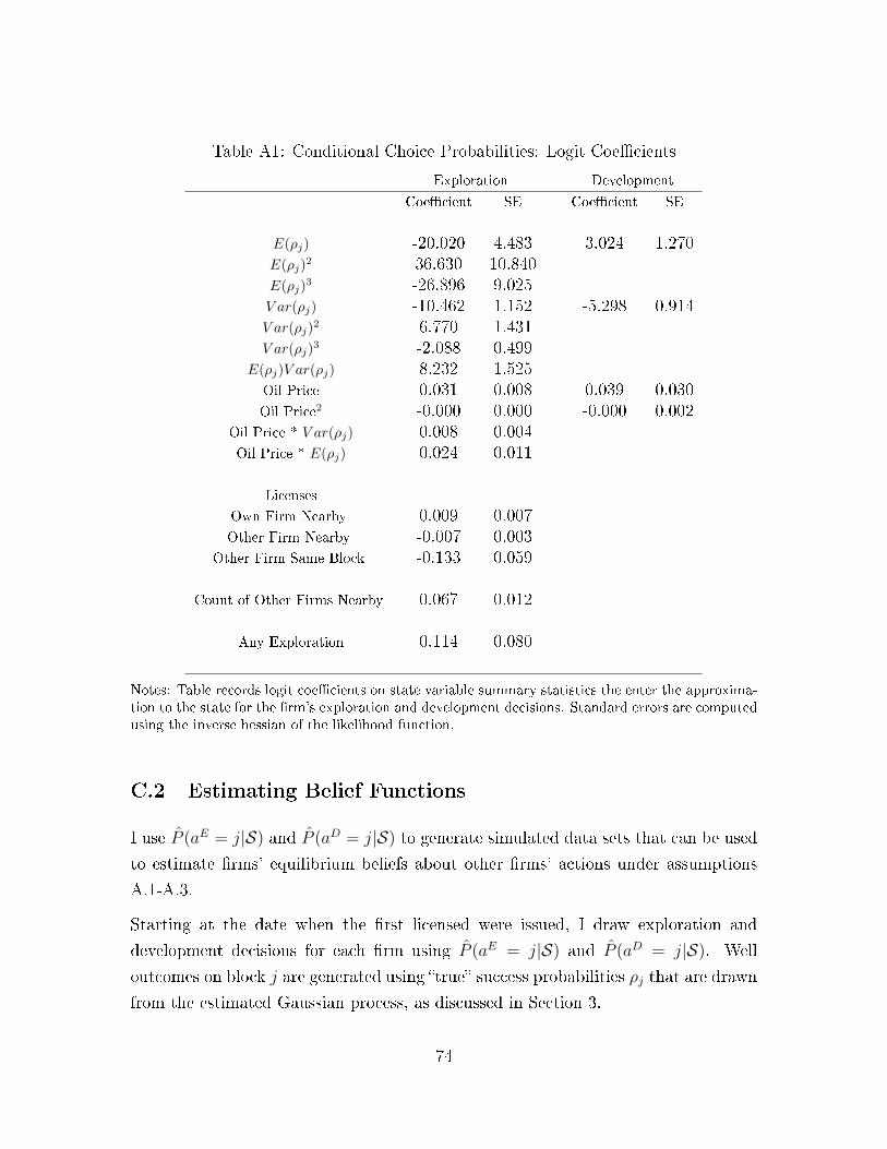
Table A1: Conditional Choice Probabilities: Logit Coecients

Exploration Development

Coecient SE Coecient SE

E(ρj) -20.020 4.483 3.024 1.270E(ρj)

2 36.630 10.840E(ρj)

3 -26.896 9.025V ar(ρj) -10.462 1.152 -5.298 0.914V ar(ρj)

2 6.770 1.431V ar(ρj)

3 -2.088 0.499E(ρj)V ar(ρj) 8.232 1.525Oil Price 0.031 0.008 0.039 0.030Oil Price2 -0.000 0.000 -0.000 0.002

Oil Price * V ar(ρj) 0.008 0.004Oil Price * E(ρj) 0.024 0.011

Licenses

Own Firm Nearby 0.009 0.007Other Firm Nearby -0.007 0.003

Other Firm Same Block -0.133 0.059

Count of Other Firms Nearby 0.067 0.012

Any Exploration 0.114 0.080

Notes: Table records logit coecients on state variable summary statistics the enter the approxima-tion to the state for the rm's exploration and development decisions. Standard errors are computedusing the inverse hessian of the likelihood function.

C.2 Estimating Belief Functions

I use P (aE = j|S) and P (aD = j|S) to generate simulated data sets that can be used

to estimate rms' equilibrium beliefs about other rms' actions under assumptions

A.1-A.3.

Starting at the date when the rst licensed were issued, I draw exploration and

development decisions for each rm using P (aE = j|S) and P (aD = j|S). Well

outcomes on block j are generated using true success probabilities ρj that are drawn

from the estimated Gaussian process, as discussed in Section 3.

74

Every period, for every well that is drilled by rm f in a period, I allow each other

rm to observe the outcome with probability α, with unobserved wells revealed at

the end of the condentiality period. At the end of each period, I update each rm's

state variable according to the new observed well outcomes and allow the price to

evolve according to the estimated random walk process. Each period, rm licenses

are set to the observed licenses in the data, unless a rm-block has been developed,

in which case the license is removed.

This simulation procedure generates a data set which records each rm's state Sftand actions (aEft, a

Dft) at each date. I simulate this data 10 times using dierent seeds

for the random number generator. Let r index simulations. I estimate the following

equations on the simulated data using logistic regression:

1(aErgt = j) = qE(Srft, g, j) + εftrj (28)

1(aErgt−τ = j) = qPast(Srft, g, j) + εftrj

1(aDrgt = j) = qD(Srft, g, j) + εftrj

Where εftrj is i.i.d. logistic. These specications are regressions of rm g's action on

rm f 's state. Data is pooled across simulations r, dates t, pairs of rms (f, g), and

locations j ∈ Jgt. In practice, I estimate these specication on a random sub-sample

of this pooled data set.

The functions qE(Srft, g, j), qPast(Srft, g, j), and qD(Srft, g, j) are linear in elements

of Srft. In particular, qPast(Srft, g, j), and qD(Srft, g, j) have the same specication

as vfE(j,S) outlined in Appendix C.1 above, where the counts of own and other

blocks now refer to rm g. That is, the functions summarize rm f 's beliefs about

the well success probability on block j and counts of rm g and other m's licenses

near block j. Likewise, qD(Srft, g, j) has the same specication as vfD(j,S).

Estimates of rms' equilibrium beliefs about other rms actions, dened in equa-

tions14 and 15, are then given by

QE(Srft, g, j) =exp(qE(Srft, g, j))

1 + exp(qE(Srft, g, j)), (29)

75

and analogously for QPast and QD.

C.3 Estimating Dynamic Parameters

In the second step, I use the estimated conditional choice probabilities P (aE = j|S)

and P (aD = j|S), estimated beliefs QE(Sft, g, j), QD(Sft, g, j), and QPast(Sft, g, j),and estimated spillover parameter, α, to estimate the cost parameters θ2. The rm's

value functions (8) can be written in terms of the expected sum of future payos and

costs as

V Eft0

(S, θ2) = E

∞∑t=t0

βt∑j=Jft

(1(aDft = j) (πj − (κ(j,Sft)− νftj))− 1(aEft = j) (c(j,Sft)− εftj)

) .(30)

Where the expectations are taken over all future cost shocks, rm actions, and re-

alizations of s(w), of (w), and πj with respect to the rm's beliefs at state S. To

estimate this expectation, I forward simulate the model from initial state S using the

CCP estimates P (aE = j|S) and P (aD = j|S) to draw rm f 's actions and estimates

of rm f 's beliefs about other rms actions QE, QD, and QPast to draw other rms'

actions.28 Simulation proceeds as follows:

1. Draw an exploration action using probabilities P (aEft = j|St). Compute ex-

pected cost shock εftaE , given realized action. If a well is drilled, let it be

successful with probability corresponding to rm f 's beliefs at state St.

2. Draw other rms' exploration actions using QE. Let wells be successful with

probability corresponding to rm f 's beliefs at state Sft.

3. Draw of (w) for wells drilled by other rms using α.

4. If t < τ draw announcement of other rms' pat wells using QPast. Let wells be

successful with probability corresponding to rm f 's beliefs at state Sft.28Hotz and Miller (1993) obtain estimates of the rm's value function using nite dependence by

normalizing one state to have a continuation value of 0. This approach is complicated here sincethe absorbing state of developing all blocks is the result of a series of choices, rather than a singlechoice that is available at every state (for example exit in a standard dynamic oligopoly model).

76

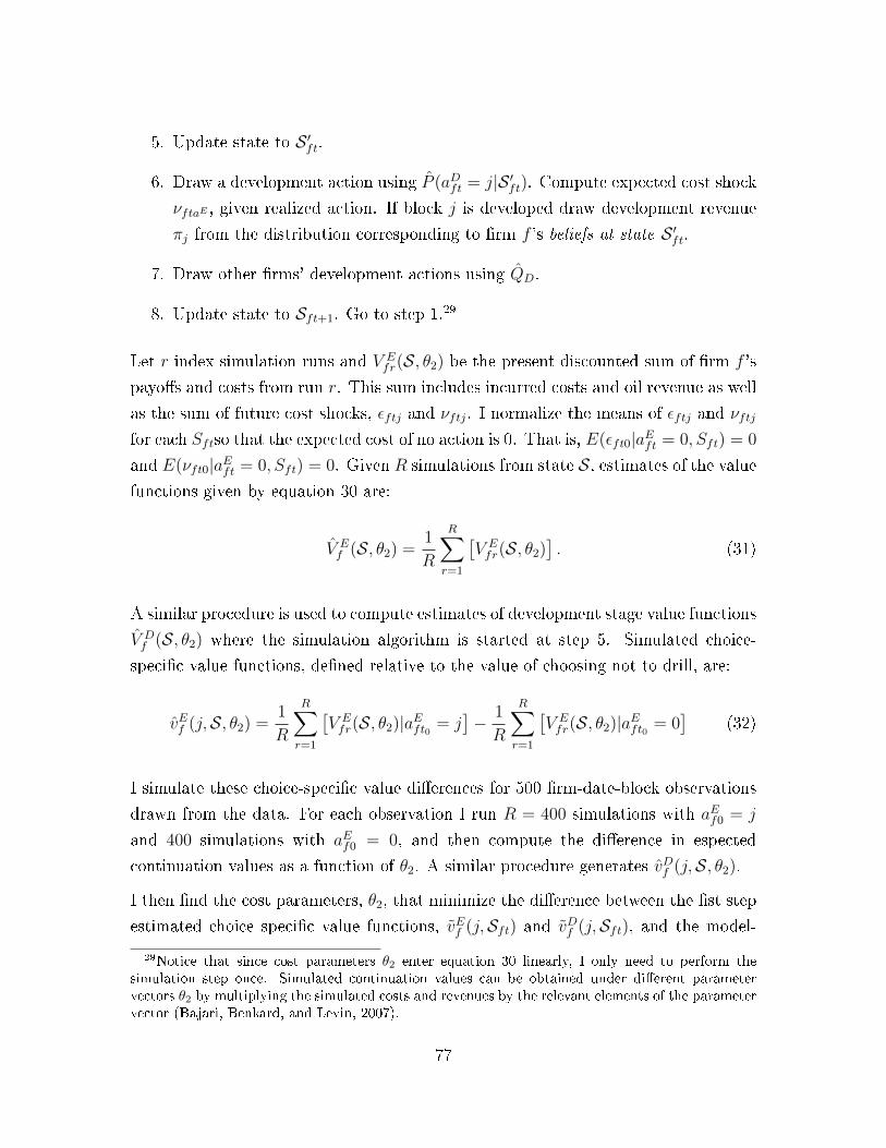
5. Update state to S ′ft.

6. Draw a development action using P (aDft = j|S ′ft). Compute expected cost shock

νftaE , given realized action. If block j is developed draw development revenue

πj from the distribution corresponding to rm f 's beliefs at state S ′ft.

7. Draw other rms' development actions using QD.

8. Update state to Sft+1. Go to step 1.29

Let r index simulation runs and V Efr(S, θ2) be the present discounted sum of rm f 's

payos and costs from run r. This sum includes incurred costs and oil revenue as well

as the sum of future cost shocks, εftj and νftj. I normalize the means of εftj and νftj

for each Sftso that the expected cost of no action is 0. That is, E(εft0|aEft = 0, Sft) = 0

and E(νft0|aEft = 0, Sft) = 0. Given R simulations from state S, estimates of the value

functions given by equation 30 are:

V Ef (S, θ2) =

1

R

R∑r=1

[V Efr(S, θ2)

]. (31)

A similar procedure is used to compute estimates of development stage value functions

V Df (S, θ2) where the simulation algorithm is started at step 5. Simulated choice-

specic value functions, dened relative to the value of choosing not to drill, are:

vEf (j,S, θ2) =1

R

R∑r=1

[V Efr(S, θ2)|aEft0 = j

]− 1

R

R∑r=1

[V Efr(S, θ2)|aEft0 = 0

](32)

I simulate these choice-specic value dierences for 500 rm-date-block observations

drawn from the data. For each observation I run R = 400 simulations with aEf0 = j

and 400 simulations with aEf0 = 0, and then compute the dierence in espected

continuation values as a function of θ2. A similar procedure generates vDf (j,S, θ2).

I then nd the cost parameters, θ2, that minimize the dierence between the st step

estimated choice specic value functions, vEf (j,Sft) and vDf (j,Sft), and the model-

29Notice that since cost parameters θ2 enter equation 30 linearly, I only need to perform thesimulation step once. Simulated continuation values can be obtained under dierent parametervectors θ2 by multiplying the simulated costs and revenues by the relevant elements of the parametervector (Bajari, Benkard, and Levin, 2007).

77

implied choice specic value functions, vEf (j,Sft, θ2) and vDf (j,Sft, θ2), using the ob-

jective function given by equation 33.

θ∗2 = arg minθ2

∑f

∑t

∑k∈E,D

(vkf (j,Sft)− vkf (j,Sft, θ2)

)2(33)

Where the sum is over the set of 500 rm-date-blocks drawn from the data.

Since the simulated value functions are non linear in simulation error, estimation

based on equation 33 is asymptotically biased if the number of simulation draws, R,

is xed (Laont, Ossard, and Vuong, 1995). To ensure consistency, it is necessary

either to add a bias correction term, or to assume that R goes to innity faster than

the square root of the number of observations (Gourieroux and Monfort, 1993) - here

the number of states included in the regression.

Standard errors for θ2 are obtained by repeating the second step estimation procedure

for 100 bootstrap draws from the rst step CCP estimated in Table A1 and taking

the standard deviation of the estimated parameters. Because the simulation of value

functions is computationally intensive, I only use 100 simulations for each bootstrap

draw.

C.4 Technical Details on Distribution of States

Dene a period t observation as

Xt = (j(w), s(w), f(w)) : t(w) < t, Jftf∈F∪0, Pt, (34)

the set of wells, the set of licenses, and the oil price. The data consists of T such

observations, X = XtTt=1. If the states Sftf∈F were uniquely identied byXt, then

P (aEf = j|S) could be estimated using a straightforward logit. This is not possible

since the econometrician does not observe the vector of . That is, the econometrician

does not know which well outcomes each rm observed in reality. Dierent realizations

of of imply dierent states through the eect of observed well outcomes on Gft. The

state variable Sft is therefore not directly observed in the data, and for every (f, t),

the data is consistent with a set of states.

78

Formally, denote a sequence of rm f states as Sf = SftTt=1. There exists a function

s(·) such that Sf = s(of |X). Dene Sf (X) as the range of this function. That is,

Sf is the set of rm f states that are consistent with the data. There also exists an

inverse correspondence s−1(Sf |X) that maps states to (possibly multiple) vectors of

that imply those states.

To recover CCP estimates, observe that dierent values of α dene distributions over

the elements of Sf . In particular, the probability of sequence of states Sf ∈ Sf ,conditional on the data is:

P (Sf |X,α) =∑

o∈s−1(Sf |X)

(α∑w o(w)(1− α)

∑w(1−o(w))

). (35)

Given this distribution over true states, the likelihood of a sequence of exploration

choice observations conditional on (X,α) is given by:

LEf =∑

Sf∈Sf (X)

T∏t=1

∏j∈Jft∪0

P (aEft = j|S)1(aEft=j)P (aDft = j|S)1(a

Dft=j)

P (Sf |X,α)

.(36)

Note that the summation in equation 36 is an expectation. In practice, it is computa-

tionally infeasible to compute the action probabilities at every possible state sequence

Sf ∈ Sf . I approximate this expectation for dierent values of α using importance

sampling, and I allow α to take values on a grid α ∈ [0.01, 0.02, ..., 0.99].

C.5 Estimation of Development Payos

Firms decide to develop blocks based on the expected payo from the block, πj and

the xed cost of developing the block, κj. πj is drawn from a distribution Γ(π; ρj, P ).

I assume that development payo is given by πj = Rjµ(P ) where Rj is the quantity

of oil reserves on block j (in barrels), and µ(P ) is a multiplier that depends on the

price per barrel. I assume that reserves are drawn from a log normal distribution:

Rj ∼ logN(αR + µRρj, σR). Note that the mean parameter depends on the true

exploration success probability of the block, ρj.

Note that I do not observe Rj directly in the data, but I do observe the realized ow

of oil from all production wells drilled from a development platform up to 2000. I

79

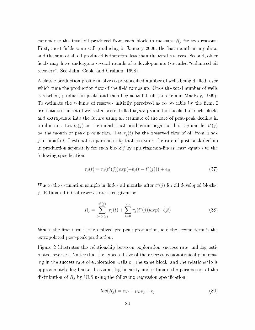
cannot use the total oil produced from each block to measure Rj for two reasons.

First, most elds were still producing in January 2000, the last month in my data,

and the sum of all oil produced is therefore less than the total reserves. Second, older

elds may have undergone several rounds of redevelopments (so-called enhanced oil

recovery. See Jahn, Cook, and Graham, 1998).

A classic production prole involves a pre-specied number of wells being drilled, over

which time the production ow of the eld ramps up. Once the total number of wells

is reached, production peaks and then begins to fall o (Lerche and MacKay, 1999).

To estimate the volume of reserves initially perceived as recoverable by the rm, I

use data on the set of wells that were drilled before production peaked on each block,

and extrapolate into the future using an estimate of the rate of post-peak decline in

production. Let t0(j) be the month that production began on block j and let t∗(j)

be the month of peak production. Let rj(t) be the observed ow of oil from block

j in month t. I estimate a parameter bj that measures the rate of post-peak decline

in production separately for each block j by applying non-linear least squares to the

following specication:

rj(t) = rj(t∗(j))exp(−bj(t− t∗(j))) + εjt (37)

Where the estimation sample includes all months after t∗(j) for all developed blocks,

j. Estimated initial reserves are then given by:

Rj =

t∗(j)∑t=t0(j)

rj(t) +∞∑t=0

rj(t∗(j))exp(−bjt) (38)

Where the rst term is the realized pre-peak production, and the second term is the

extrapolated post-peak production.

Figure 2 illustrates the relationship between exploration success rate and log esti-

mated reserves. Notice that the expected size of the reserves is monotonically increas-

ing in the success rate of exploration wells on the same block, and the relationship is

approximately log-linear. I assume log-linearity and estimate the parameters of the

distribution of Rj by OLS using the following regression specication:

log(Rj) = αR + µRρj + εj (39)

80

Where εj ∼ N(0, σR) and I measure ρj using the realized pre-development exploration

well success rate on block j. The estimated parameters are reported in Table A2.

Finally, note that πj = RjP (1 − 0.125) 1−β30

30(1−β)(1 − µ) This multiplier converts the

total reserves in barrels to the present discounted value of revenue at the current

price level, less the 12.5% royalty paid to the government, where oil is assumed to

ow at a constant rate for 40 years, at which point the reserves, Rj are exhausted.

µ ∈ [0, 1] is a parot margin parameter that represents the share of revenues after

the royalty tax that are captured by operating costs. This parameter is not identied

by the data, and I normalize it to 20%. Changing this parameter would change the

estimated cost parameters proportionally and have no eect on rm choices.

Table A2: Distribution of Development Payos

Parameter Estimate SEαR 1.594 0.420µR 5.990 0.964σ2R 1.949 0.115

N 80

Notes: Reported coecients are from OLS estimation of regression specication given by equation39. Sample includes one observation for each of the 80 blocks developed before 2000 in the areanorth of 55N and east of 2W . Left hand side variable is the log of the predicted oil reserves onblock j, measured in millions of barrels. Right hand side variable is the observed exploration wellsuccess rate for block j calculated using all exploration wells drilled on block j before development.

C.6 Estimation of License Issuing Process

New drilling licenses are issued by the government in rounds that occur irregularly

every two to three years. To model this process, I asusme that licensing rounds

happen each month with a probability 1/24, so that every two years there is one

round in expectation. When a round takes place, new licenses are issued and existing

licenses may be revoked. Firm f has correct beliefs about this process

In a given round, one license can be issued on each block j. The probability that a

new license on block j is issued to a rm f is given by:

P (j ∈ Jft) =exp(βZfjt)

1 +∑

g:j /∈Fjt exp(βZgjt)

81

That is, a new license can be issued to any rm that does not already have a license on

that block. The probability of receiving the license depends on covariates Zfjt which

include whether any rm has a license on the block at date, whether any neighboring

blocks are licensed at date, and whether any neighboring blocks are licensed to rm

f .

After new licenses are issued, existing licenses are revoked at random with probability

ω.

I estimate this licensing process by running a regression of licenses at date t on

covariates Zfjt−24. That is, I estimate the probability that a new license is issued in

today as a function of the license distribution two years ago. Similarly, I estimate ω

as the probability that a license at date t is revoked by date t + 24. The estimated

parameters recorded in Table A3.

Table A3: License Issuing Process

Probability of New License Probability of Revoked License

Constant -6.735 ω 0.173(0.009) (0.000)

Licensed in t− 24 -0.578(0.015)

Neighbors Licensed to g 6= f in t− 24 -0.127(0.067)

Neighbors Licensed to f in t− 24 2.181(0.020)

D Identication Details

In this section I provide a proof of identication of the exploration conditional choice

probabilities (CCPs) P (aEf = j|S) and the information spillover parameter, α. Iden-

tical reasoning applies to development choice probabilities. Let X be the space of

possible data points, where X ∈X is an observation as dened by equation 34.

Proposition 4. Suppose P (aEf = j|Sf (X)) is observed for all f and all X ∈ X.

These observed probabilities are consistent with a unique value of α and a unique

value of P (aEf = j|Sf ) for every possible state Sf .

82

Proof. First, suppose that α is known.

Let wt be a vector of length W = |w : t(w) < t| indexed by i ∈ [1, ...,W ] is an

index which contains the identity w of each well w ∈ w : t(w) < t in some order

such that we can refer to well identities by, wt(i) . Let γft be a vector of length W

with ith element γft(i) = 1(f(wt(i)) = f). γft is a vector of indicators for whether

each well w was drilled by rm f .

We can then rewrite the observable data Xt as Xt = xt, γftf∈F. Where

xt = (j(w), s(w)) : t(w) < t, Jftf∈F∪0, Pt.

xt describes the location and outcome of all wells drilled up to date t, the date t

distribution of licenses, and the oil price.

Dene oft as a vector of length W with ith element given by oft(i) = of (wt(i)). oft

is just an ordered vector of containing indicators for whether rm f observed each

well w ∈ w : t(w) < t (a subset of the elements of of ).

Suppose for simplicity that all wells w, t − t(w) < τ , so no wells are older than

the condentiality period τ . This assumption simplies notation, and the following

argument easily generalizes. I now drop the t subscript for simplicity.

Firm f 's state is uniquely dened by the pair (of , x). That is, there exists a function

Sf = s(f,of , x). The set of states that are consistent with the objects observed in

the data is dened by a correspondence Sf = s(f,γf , X). In particular:

s(f,γf , x) = s(f,of , x) : γf (i) = 1⇒ of (i) = 1∀i ∈ [1, ...,W ].

So s(f,γf , x) contains states implied by all possible values of of . In particular, each

well drilled by a rm other than f may or may not have been observed.

Now x a value of x. There are 2W possible values of γf and therefore of Sf =

s(f,γf , x). There are also 2W possible values of of and therefore of Sf = s(f,of , x).

Let Sf (x) be the set of possible values of Sf and Sf (x) be the set of possible values

of Sf . For any action choice j ∈ Jf and any Sf ∈ Sf (x) we can write:

P (aEf = j|Sf ) =∑

Sf∈Sf (x)

P (aEf = j|S)P (Sf |Sf ).

83

Where P (Sf |Sf ) is a function of α given by equation 35 if Sf ∈ Sf and P (S|Sf ) = 0

if Sf /∈ Sf .

There are 2W such equations which dene a linear system P = AP where P is a

2W × 1 vector which stacks the probabilities P (aEf = j|Sf ), P is a 2W × 1 vector

which stacks the probabilities P (aEf = j|S), and A is a 2W × 2W matrix containing

the probabilities P (Sf |Sf ) which are known functions of α. P is observed in the data.

A is a known function of the single parameter α. P is an unknown vector for which

we would like to solve.

The vector of true CCPs P can be recovered from the observed probabilities, P

when A has full rank. This is the case here because the system of equations can be

written such that A is lower triangular with non-zero diagonal elements. I show this

by providing an algorithm to solve the system by forward substitution, which is only

possible in a triangular system of equations. The algorithm proceeds as follows:

1. Denote the vector with all entries equal to 1 by 1 Start with γ1f = 1. Let

S1f = s(f,1, x) and S1

f = s(f,1, x) . Notice S1f = S1

f . If all wells were drilled by

rm f , then they are all observed. Therefore

P (aEf = j|S1f ) = P (aEf = j|S1

f ).

P (aEf = j|S1f ) is uniquely identied.

2. Denote the vector with all entries except the ith equal to 1 and the ith equal

to 0 by 1i. Let γ2f = 1i. Let S2

f = s(f,1i, x) and S2f = s(f,1i, x) .

Notice that S2f = S1

f ,S2f. The rm either did or did not observe the ith well.

Therefore

P (aEf = j|S2f ) = αP (aEf = j|S1

f ) + (1− α)P (aEf = j|S2f ).

Since the other terms are already known, P (aEf = j|S2f ) is uniquely identied.

3. Repeat step 2 for each index ∀i ∈ [1, ...,W ].

4. Proceed to vectors γf with two entries equal to 0 and repeat step 2.

5. Continue iterating through vectors with increasingly more entries equal to 0

until P (aEf = j|Sf ) has been solved for for all Sf ∈ Sf (x).

84

This algorithm generates the unique solution P of the system of equations P = AP .

This can be repeated for any value of x.

Now I argue that α is uniquely identied. Fix a pair (x, x′) where x and x′are identical

except for the outcome of the ith well. The following four equations hold:

P (aEf = j|s(f,1, x)) = P (aEf = j|s(f,1, x))

P (aEf = j|s(f,1, x′)) = P (aEf = j|s(f,1, x′))

P (aEf = j|s(f,1i, x)) = αP (aEf = j|s(f,1, x)) + (1− α)P (aEf = j|s(f,1i, x))

P (aEf = j|s(f,1,i x′)) = αP (aEf = j|s(f,1, x′)) + (1− α)P (aEf = j|s(f,1i, x′))

The left hand side of each equation is observed. Notice that P (aEf = j|s(f,1i, x)) =

P (aEf = j|s(f,1i, x′)) since when the ith well is unobserved the two states are

identical to the rm. There are therefore three unknown choice probabilities and

the parameter α on the right hand side. α can be solved for in terms of observed

quantities.

E Simulation Details

In this section, I describe the simulation algorithm used to compute counterfactual

equilibria of the estimated model. Inputs to the simulation are a vector of model

parameters, θ, a condentiality window, τ , a license assignmentJftf∈F for each

period, rst step conditional choice probability (CCP) estimates, P (aE = j|S) and

P (aD = j|S), and belief functions QE, QD, and QPast. The output of the simulation

are equilibrium CCPs, P ∗(aE = j|S) and P ∗(aD = j|S).

The algorithm works by taking a set of CCPs as input and forward simulating those

probabilities to obtain model-implied choice specic continuation values (given by

equation 31). This is the same procedure as used in the second step of estimation, as

described in Appendix C.3.

These value functions imply new choice probabilities that can be used to generate

simulated data, from which new belief functions can be estimated (using the proce-

dure described in Appendix C.2). The procedure can then be iterated until choice

probabilities converge to a xed point.

85

The algorithm proceeds as follows:

1. Fix a set of states, S and use rst step CCPs P (aE = j|S) and P (aD =

j|S) and rst step estimates of QE, QD, and QPast to perform the forward

simulation described in Appendix C.3 for each S ∈ S. This procedure generatesmodel implied exploration and development probabilities, P 1(aEf = j|S, θ2) andP 1(aDf = j|S, θ2).

2. Simulate data using P 1(aEf = j|S, θ2) and P 1(aDf = j|S, θ2), and use this data

to estimate belief functions, QE1, QD1, and QPast1 .

3. Go back to step 1 and repeat using new exploration CCPs and belief functions.

Repeat for k iterations until

∑S∈S

(P k(aEf = j|S, θ2)− P k+1(aEf = j|S, θ2)

)2≈ 0

and ∑S∈S

(P k(aDf = j|S, θ2)− P k+1(aDf = j|S, θ2)

)2≈ 0.

In practice I modify this algorithm by terminating the forward simulation in iteration

k after 48 months and assigning terminal continuation values V k−1(S, θ2) from the

k − 1th iteration, extrapolated across states using a linear regression in elements of

S. This greatly reduces the time it takes to perform one iteration (from > 10 hours

to ∼ 2 hours).

F License Clustering Algorithm

In this section I describe the algorithm used to generate the clustered license assign-

ment. Let Jfyf∈F be the license assignment at the end of year y. Let Jy be the set

of licenses that were issued in year y. An element of Jy is a triple (Xj, t1, t2) where

Xj identies the block coordinates, t1 is the start date and t2 is the end date of the

license as observed in the data. Let Jfy ⊂ Jy be the set of subset of year y licenses

that were assigned to rm f in the data. Finally, let J ′fyf∈F be the counterfactual

license assignment for year y.

86

Licenses and rms have preferences over each other given by a distance metric, Ωfjy.

The distance metric is chosen such that new licenses want to be assigned to rms

which hold a larger number of nearby licenses, and rms want to be assigned the

licenses that are close to many of their existing licenses. In particular,

Ωfjy =∑

k∈J ′fy−1

exp (−|Xk −Xj|) . (40)

Notice that Ωfjy is increasing in the number of licenses held by f at a given distance

from block j, and decreasing in the distance of any one license from block j, holding

the locations of the other licenses xed.

The algorithm proceeds as follows.

1. Start with the initial assignment J ′f0f∈F = Jf0f∈F .

2. Let F0 be the set of rms for which J ′f0 6= . Let F−0 = F\F0.

3. Run a deferred acceptance matching algorithm between the set of rms F0 and

the set of licenses J1. Each rm f ranks blocks according to a distance metric

Ωfj1. Each license j ranks rms according to Ωfj1. Each license j can only be

matched to one rm. Each rm has a quota given by Qf1 = |Jf1|.

(a) Each license j proposes to its highest ranked rm.

(b) Firm f accepts the highest ranked Qf1 licenses from those that propose to

it. If fewer than Qf1 licenses propose to it it accepts all of them. Licenses

that are not accepted are rejected.

(c) Rejected licenses propose to their second highest ranked rm.

(d) Firm f accepts the highest ranked Qf1 licenses from those that propose to

it and those that it has already accepted. Licenses that are not accepted

are rejected (including those previously accepted).

(e) Repeat until all licenses are either accepted by some rm or have been

rejected by all rms.

(f) For each rm f ∈ F0, the set of licenses that were accepted is then J ′f1.

4. Denote the licenses rejected at year 1 by JR1 .

87

5. Take the rm f ∈ F−0 with the largest quota, Qf1. Assign rm f a random

license j ∈ JR1 . Compute Ωfj1 for the remaining licenses given this assignment.

6. Assign rm f its Qf1 − 1 top ranked licenses. The set of licenses assigned in

then J ′f1. Repeat steps 5 and 6 for all other rms f ∈ F−0 in order of quota

size. This approach to modeling beliefs is restrictive insofar as the variables

that enter Sf do not include all informationally relevant state variables that are

potentially observed by the rm. This can be thought of as a bounded ratio-

nality assumption that restricts the set of objects on which rms can condition

their beliefs.

7. Repeat for each year.

The algorithm generates a license assignment that holds xed the number of blocks

assigned to each rm each year and the length that each license was active. The

average number of nearby own-rm blocks is higher and the average number of nearby

other-rm blocks is lower under the clustered license assignment. I do not claim that

this assignment is in any way optimal, but this algorithm provides a method for

systematically assigning blocks to rms in a way that increases the average number

of same-rm neighbors.

88

G Additional Tables and Figures

Table A4: Regressions of Exploration Probability on Equity Holders' Nearby Licenses

Exploration Well

BlocksOwnfjt 2.467*** 2.479*** 2.505*** 2.401***

(.875) (0.858) (.851) (.868)

BlocksOpEquityfjt -.514 . . -1.026(1.277) . . (1.304)

BlocksEquityOpfjt . 1.351 . 1.220

. (0.824) . (.816)

BlocksEquityEquityfjt . . .846 .902

. . (.617) (.623)

N 80562 80562 80562 80562

Firm-Block, and Month FE Yes Yes Yes Yes

Coecients Scaled by 103 Yes Yes Yes Yes

Notes: Each column records OLS estimates of the coecients from a regression of Explorefjt oncounts on of nearby licenses (1st and 2nd degree neighbors). BlocksOpEquityfjt is the number ofblocks nearby block j at month t on which rm f , the operator of block j, is an equity holder butnot an operator. BlocksEquityOpfjt is the count of blocks nearby block j at date t for which one ofthe non-operator rms with equity on block j is the operator. BlocksEquityEquityfjt is the countof blocks nearby block j at date t for which one of the non-operator rms with equity on block j isa non-operator equity holder. Regressions also include controls for past well results as in equation6 Standard errors clustered at the rm-block level. *** indicates signicance at the 99% level. **indicates signicance at the 95% level. * indicates signicance at the 90% level.

89

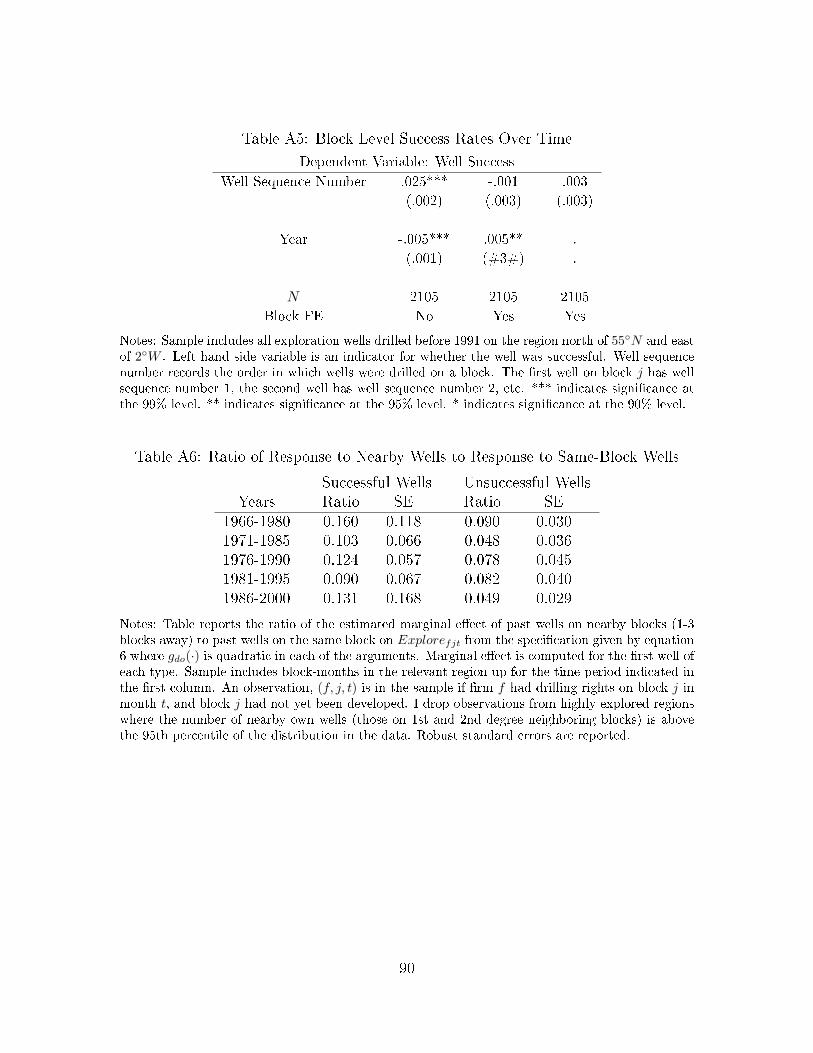
Table A5: Block Level Success Rates Over Time

Dependent Variable: Well Success

Well Sequence Number .025*** -.001 .003

(.002) (.003) (.003)

Year -.005*** .005** .

(.001) (#3#) .

N 2105 2105 2105

Block FE No Yes Yes

Notes: Sample includes all exploration wells drilled before 1991 on the region north of 55N and eastof 2W . Left hand side variable is an indicator for whether the well was successful. Well sequencenumber records the order in which wells were drilled on a block. The rst well on block j has wellsequence number 1, the second well has well sequence number 2, etc. *** indicates signicance atthe 99% level. ** indicates signicance at the 95% level. * indicates signicance at the 90% level.

Table A6: Ratio of Response to Nearby Wells to Response to Same-Block Wells

Successful Wells Unsuccessful WellsYears Ratio SE Ratio SE

1966-1980 0.160 0.118 0.090 0.0301971-1985 0.103 0.066 0.048 0.0361976-1990 0.124 0.057 0.078 0.0451981-1995 0.090 0.067 0.082 0.0401986-2000 0.131 0.168 0.049 0.029

Notes: Table reports the ratio of the estimated marginal eect of past wells on nearby blocks (1-3blocks away) to past wells on the same block on Explorefjt from the specication given by equation6 where gdo(·) is quadratic in each of the arguments. Marginal eect is computed for the rst well ofeach type. Sample includes block-months in the relevant region up for the time period indicated inthe rst column. An observation, (f, j, t) is in the sample if rm f had drilling rights on block j inmonth t, and block j had not yet been developed. I drop observations from highly explored regionswhere the number of nearby own wells (those on 1st and 2nd degree neighboring blocks) is abovethe 95th percentile of the distribution in the data. Robust standard errors are reported.

90

Table A7: Regressions of Drilling Probability on Nearby Licenses

Exploration Well

log(BlocksOwnfjt) 0.002 0.009 0.028**

(0.002) (0.014) (0.014)

log(BlocksOtherfjt) 0.015*** -0.008* -0.013***

(0.002) (0.005) (0.004)

N 21,618 21,618 21,618

Licensing Round Fixed Eects No Yes Yes

Well Outcome Controls No No Yes

Notes: Standard errors clustered at the rm-block level. Observations are at the (f, j, t) level.Sample includes all (f, j, t) observations that are within 4 months of a licensing round, for which therm f has held a license on block j for at least 6 months. Licensing rounds are identied as (f, j, t)observations for which the total number of licensed blocks neighboring block j increases from theprevious month. Block counts are of all licenses on block j and neighboring blocks on date t. Welloutcome controls are the same as in specication 6. *** indicates signicance at the 99% level. **indicates signicance at the 95% level. * indicates signicance at the 90% level.

Figure A1: Top 25 Firms

05,0

00

10,0

00

15,0

00

20,0

00

Blo

ck−

Month

s

SH

ELL

AM

OC

O

BP

TO

TA

L

PH

ILLIP

S

CO

NO

CO

TE

XA

CO

HA

MIL

TO

N

CH

EV

RO

N

MO

BIL

HE

SS

AR

PE

T

ELF

BU

RM

AH

CN

R

OP

A

AG

IP

CA

LE

DO

NIA

GU

LF

MA

RA

TH

ON

MU

RP

HY

AR

CO

PLA

CID

PR

EM

IER

BR

ITO

IL

OT

HE

R

Notes: Figure plots the number of block-month pairs for 1964-1990 licensed to each of the top 25rms, and the set of all other rms.

91

Figure A2: Gaussian Process Draws

0 20 40 60 80 100

X

0

0.1

0.2

0.3

0.4

0.5

0.6

0.7

0.8

0.9

1

(X)

Notes: Figure plots two draws (solid lines) from a logistic Gaussian process with parameters µ = 0,ω = 5, and ρ = 5 on a one-dimensional space. The dashed line corresponds to the prior mean.

Figure A3: Gaussian Process Learning

0 20 40 60 80 100

0.3

0.35

0.4

0.45

0.5

0.55

0.6

0.65

0.7

0 20 40 60 80 100

0.25

0.26

0.27

0.28

0.29

0.3

0.31

0.32

0.33

0.34

0.35

Expected Probability Standard Deviation of Probability

Notes: The x-axis of both panels represents the one dimensional space [0, 1] on which the Gaussianprocess is dened. The dashed yellow line in the left panel plots the expected value of ρ(X) for X ∈[0, 1] under prior beliefs represented by a logistic Gaussian process dened according to equations 1 -2 with µ(X) = 1 and ω = 5. The solid blue line in the left panel represents the posterior expectationof ρ(X) after observing a successful well at X = 60 and an unsuccessful well at X = 30 when ` = 15.The dotted red line represntes the posterior expectation when ` = 5. The right panel plots thestandard deviation of ρ(X) under the same prior (red dashed line) and posterior (solid blue line)beliefs.

92

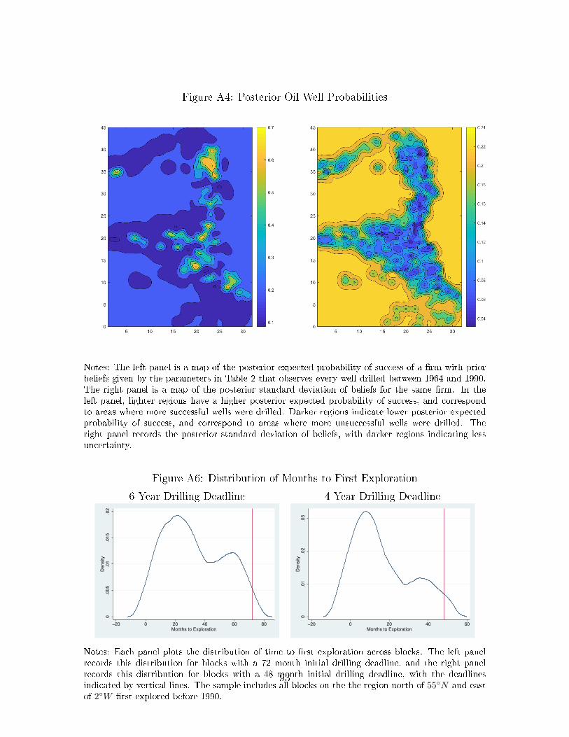
Figure A4: Posterior Oil Well Probabilities

Notes: The left panel is a map of the posterior expected probability of success of a rm with priorbeliefs given by the parameters in Table 2 that observes every well drilled between 1964 and 1990.The right panel is a map of the posterior standard deviation of beliefs for the same rm. In theleft panel, lighter regions have a higher posterior expected probability of success, and correspondto areas where more successful wells were drilled. Darker regions indicate lower posterior expectedprobability of success, and correspond to areas where more unsuccessful wells were drilled. Theright panel records the posterior standard deviation of beliefs, with darker regions indicating lessuncertainty.

Figure A6: Distribution of Months to First Exploration

6 Year Drilling Deadline 4 Year Drilling Deadline

0.0

05

.01

.015

.02

Density

−20 0 20 40 60 80Months to Exploration

0.0

1.0

2.0

3D

ensity

−20 0 20 40 60Months to Exploration

Notes: Each panel plots the distribution of time to rst exploration across blocks. The left panelrecords this distribution for blocks with a 72 month initial drilling deadline, and the right panelrecords this distribution for blocks with a 48 month initial drilling deadline, with the deadlinesindicated by vertical lines. The sample includes all blocks on the the region north of 55N and eastof 2W rst explored before 1990.

93

Figure A5: Eect of Well Age on Exploration

−.0

02

−.0

01

0.0

01

.002

.003

Effect of M

ovin

g a

Successfu

l O

ther−

Firm

Well

Back in T

ime b

y >

6 M

onth

s

0 2 4 6 8 10Well Age (Years)

Notes: Figure plots OLS estimates of coecients from a specication 6 with additional controls forthe number of past successful other-rm wells 1-3 blocks away and more than T months old (SucT )and the number of such wells more than T − 6 months old (SucT−6). Each point is the coecienton SucT for a dierent regression, where the denition of T is given by the x-axis. For example, therst point plots the eect of increasing the number of successful other rm wells more than 1 yearold, holding xed the total number of past successful wells and the number of past successful wellsmore than 6 months old. It can therefore be interpreted as the eect of moving a well drilled 6-12months ago back in time so it is more than 12 months old. Solid lines indicate a 95% condenceinterval computed using robust standard errors. Vertical line indicates 5 year expiry date for wellcondentiality.

94

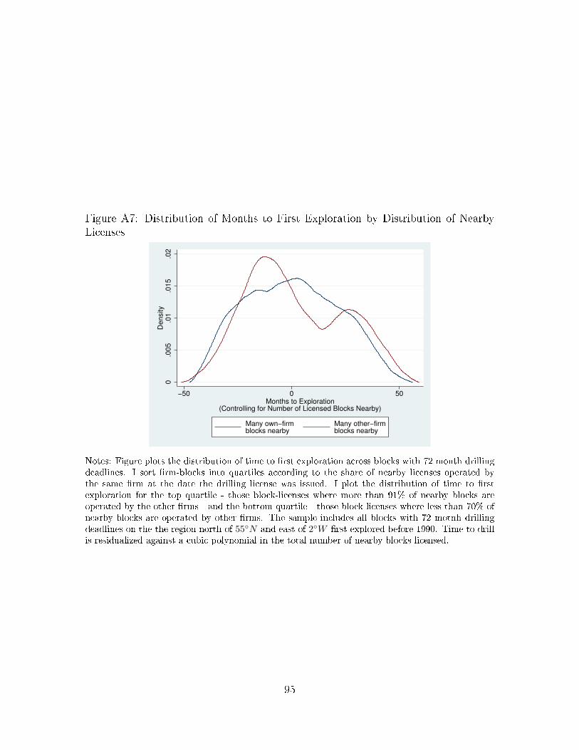
Figure A7: Distribution of Months to First Exploration by Distribution of NearbyLicenses

0.0

05

.01

.015

.02

Density

−50 0 50Months to Exploration

(Controlling for Number of Licensed Blocks Nearby)

Many own−firmblocks nearby

Many other−firmblocks nearby

Notes: Figure plots the distribution of time to rst exploration across blocks with 72 month drillingdeadlines. I sort rm-blocks into quartiles according to the share of nearby licenses operated bythe same rm at the date the drilling license was issued. I plot the distribution of time to rstexploration for the top quartile - those block-licenses where more than 91% of nearby blocks areoperated by the other rms - and the bottom quartile - those block-licenses where less than 70% ofnearby blocks are operated by other rms. The sample includes all blocks with 72 motnh drillingdeadlines on the the region north of 55N and east of 2W rst explored before 1990. Time to drillis residualized against a cubic polynomial in the total number of nearby blocks licensed.

95

Figure A8: Maps of Early Exploration

1969 1970

1971 1972

1973 1973

Notes: Each map plots the location of exploration wells drilled that year. Red points are unsuccessfulwells and green points are successful wells.

96