Information Asymmetry and the Value ... - Corporate … · assumption of perfect capital markets,...
55
Information Asymmetry and the Value of Cash * Matthias C. Gr¨ uninger † Simone Hirschvogl ‡ First Draft: February, 2007 This Draft: April, 2008 Abstract This paper investigates the value of cash for a broad international sample consisting of 7,474 firms from 45 countries over the 1995 to 2005 period. In contrast to previous pa- pers which mostly focus on the marginal value of cash with respect to different corporate governance regimes, we study the marginal value of cash in connection with firm-specific and time-varying information asymmetry. We test two contradictory hypotheses. Accord- ing to the pecking order theory, asymmetric information leads to adverse selection and provides a value-increasing role for internal funds. However, the free cash flow theory predicts that abundant cash bundled with asymmetric information leads to moral hazard and consequently to a lower marginal value of cash. Our results indicate that informa- tion asymmetry decreases the marginal value of cash and thus strongly support the free cash flow theory. This evidence is further emphasized by splitting the data according to governance measures. Keywords: Information asymmetry, cash holdings, value of cash, analysts’ forecasts JEL classification: G32 * We would like to thank Marco Becht, Francesca Cornelli, Wolfgang Drobetz, Daniel H¨ ochle, Ben Jann, Dave Yermack, Josef Zechner and workshop participants at the University of Basel, University of Vienna, and CFS Summer School in Eltville 2007 for helpful comments. All errors remain our own. † Department of Corporate Finance, University of Basel, Petersgraben 51, 4003 Basel, Switzerland. Mail: [email protected] ‡ Department of Finance, University of Vienna, Br¨ unnerstrasse 72, 1210 Vienna, Austria. ECARES, Univer- sit´ e Libre de Bruxelles, Avenue F.D. Roosevelt 50, CP 114, 1050 Brussels, Belgium. Early Stage Researcher, ECGTN. Mail: [email protected]
Transcript of Information Asymmetry and the Value ... - Corporate … · assumption of perfect capital markets,...

Information Asymmetry and the Value of Cash∗
Matthias C. Gruninger † Simone Hirschvogl ‡
First Draft: February, 2007
This Draft: April, 2008
Abstract
This paper investigates the value of cash for a broad international sample consisting of7,474 firms from 45 countries over the 1995 to 2005 period. In contrast to previous pa-pers which mostly focus on the marginal value of cash with respect to different corporategovernance regimes, we study the marginal value of cash in connection with firm-specificand time-varying information asymmetry. We test two contradictory hypotheses. Accord-ing to the pecking order theory, asymmetric information leads to adverse selection andprovides a value-increasing role for internal funds. However, the free cash flow theorypredicts that abundant cash bundled with asymmetric information leads to moral hazardand consequently to a lower marginal value of cash. Our results indicate that informa-tion asymmetry decreases the marginal value of cash and thus strongly support the freecash flow theory. This evidence is further emphasized by splitting the data according togovernance measures.
Keywords: Information asymmetry, cash holdings, value of cash, analysts’ forecasts
JEL classification: G32
∗We would like to thank Marco Becht, Francesca Cornelli, Wolfgang Drobetz, Daniel Hochle, Ben Jann,Dave Yermack, Josef Zechner and workshop participants at the University of Basel, University of Vienna, andCFS Summer School in Eltville 2007 for helpful comments. All errors remain our own.†Department of Corporate Finance, University of Basel, Petersgraben 51, 4003 Basel, Switzerland. Mail:
[email protected]‡Department of Finance, University of Vienna, Brunnerstrasse 72, 1210 Vienna, Austria. ECARES, Univer-
site Libre de Bruxelles, Avenue F.D. Roosevelt 50, CP 114, 1050 Brussels, Belgium. Early Stage Researcher,ECGTN. Mail: [email protected]

1 Introduction
JP Morgan economists have calculated that savings by companies in rich countries increased
by more than $1 trillion from 2000 to 2004 and measured against the last 40 years companies
have never hoarded so much cash as they do today.1
By observing this corporate behavior, a natural question to ask is which factors lead firms
to accumulate such enormous amounts of funds. Finding possible answers to this conundrum
is especially enlightening as the benchmark textbook model would tell us that under the
assumption of perfect capital markets, cash holdings are irrelevant to the firm. The reason is
that in this idealized situation external finance can always be obtained at fair terms. However,
by looking at figures from the corporate landscape, the irrelevancy of cash is not supported. For
example, the U.S. software giant Microsoft presented in its 2004 annual report a cash position
amounting to $60.6 billion. However, amid growing investor pressure, Microsoft announced
in July 2004 that it would pay a one-time dividend of $32 billion in 2004 and buy back up to
$30 billion of the company’s stock over the next four years. Upon the arrival of that news,
Microsoft’s stock price rose by 5.7% in the after-trading which exemplifies that cash can by
no means be regarded as irrelevant in investors’ eyes.2
Hence, in order to depict the current business setting some of the assumptions of perfect capi-
tal markets have to be relaxed. First, if transaction costs are incorporated into the model, an
optimal cash balance will be determined and the irrelevancy of cash does not hold anymore.
Second, if information asymmetry (henceforth referred to as IA) is considered in the analy-
sis, adverse selection and moral hazard problems result. Focusing on adverse selection, the
underlying model dates back to Myers and Majluf (1984), who explicitly consider the role of
cash holdings in the presence of IA. Adverse selection leads managers to abstain from raising
external capital as they are not willing to issue undervalued securities. Therefore, a cash buffer
can prevent the management from being forced to pass up positive NPV projects. However,
there are two sides to everything. In this respect, Jensen (1986) analyzes the agency costs of
1 JPMorgan Research: Corporates are driving the global saving glut, June 24, 2005.2 The Wall Street Journal, Microsoft to Dole Out its Cash Hoard, July 21, 2004, p. A.1.
1

free cash flow and hence focuses on the dark side of cash holdings. His framework is based on
moral hazard. Instead of paying out free cash flow to the capital providers, managers waste
the funds on inefficient investments or on their own pet projects.
From the preceding discussion, it becomes obvious that cash holdings and IA are interrelated.
This means that studying corporate cash holdings with an emphasis on IA could provide
valuable insights into the firms’ motivation to hold cash. This is exactly the novel path that
our study takes and contributes to the literature. The existing cash literature can loosely
be divided into two different strands. The first category examines the determinants of cash
holdings and whether there exists an optimal amount from the perspective of the shareholders.
The second approach focuses on the impact of liquidity on firm performance and firm valuation.
Importantly, the empirical study presented in this chapter belongs to the second category.
Potentially, it would be interesting to follow the first path and analyze how a firm’s cash reserve
is influenced by the level of IA. Yet, it is virtually impossible to derive clear predictions and to
unambiguously interpret the results from following this path: On the one hand, according to
the pecking order theory a firm should hold more money when the level of IA is higher, because
financial slack is valuable. On the other hand, this argument is especially important for firms
with greater investment opportunities and according to the pecking order firms should use cash
in the first place. Thus, depending on the stance one adopts completely opposite predictions
for the influence of IA on the level of cash can be derived. The free cash flow problem leads
to similar ambiguous predictions. One can argue that firms with a higher degree of IA hold
more cash, because the management is very reluctant to distribute excess cash to shareholders.
However, it also can be argued that IA results in lower cash holdings, because the management
can easily dissipate cash. These difficulties of formulating clear predictions explain why we
follow the second strand of literature and investigate the influence of IA on the value of cash
and not on the level of the liquidity. Specifically, we study the value implications of cash
holdings under consideration of firm-specific time-varying IA.
We consider this approach to be a novel path as we analyze the value implications of cash
holdings from a different angle. Although in the past researchers have already investigated
the value consequences of corporate cash holdings, they did so with respect to corporate gov-
2

ernance issues and not with an emphasis on IA. In this strand of literature, most authors
find that a low corporate governance regime has detrimental effects on the value of corporate
liquidity holdings (see, for example, Dittmar et al., 2003; Pinkowitz et al., 2006; Dittmar and
Mahrt-Smith, 2007). However, we think it is very illuminating to focus on IA as another
channel where corporate cash holdings can have benefits in line with the Myers and Majluf
(1984) argument (as external capital is costly) and/or also costs according to Jensen (1986)
(as increased managerial discretion could lead managers to squander corporate liquidity re-
sources). We empirically test the two hypotheses and investigate which effect outweighs the
other. In this respect, our sample is very extensive encompassing 7,474 firms from 45 coun-
tries for the period 1995 to 2005, which is equal to 42,476 firm-year observations. We also
employ different estimation methods. Specifically, the results are calculated via fixed effects
estimation techniques and also with the Fama-MacBeth procedure. We derive our results for
the actual cash ratio and also with the help of an estimated metric called ‘excess cash’.
Considering the actual cash ratio, our results reveal that the marginal value of cash (without
considering IA) is on average around one dollar. However, by incorporating IA (dispersion of
analysts’ earnings forecasts), the marginal value of cash incurs a substantial valuation discount
and is significantly decreased. This evidence provides an initial corroboration of the free cash
flow argument by Jensen (1986). For our data set it seems to hold that the agency costs
due to moral hazard tend to outweigh the benefits due to the availability of internal funds.
However, in order to distinguish more precisely between our two opposing hypotheses, we split
the sample according to governance and financing constraints measures. In this respect, we
find that the value of cash is higher if governance is stronger which further emphasizes the
free cash flow argument. On the other hand, the results based on the financing constraints
measures do not paint a clear picture and hence no clear-cut conclusions can be drawn. As a
robustness test of the results using the actual cash-ratio we derive a measure for excess cash
based on Opler et al. (1999). Importantly, the results remain qualitatively the same for this
different metric.
Taken together, the results have important implications and question generally accepted prin-
ciples of the capital structure and the cash literature. We find no evidence that financial slack
3

is valuable as predicted by the pecking order theory. From this it follows that it is not in the
shareholders’ interest that firms hold cash reserves because of IA. Hence, the precautionary
motive to hold cash appears to be questionable. However, our findings do not contradict the
pecking order theory in general. We do not argue that firms should not use internal funds
in the first place, but we argue that firms should not accumulate cash with the intention to
avoid external finance in the future.
This chapter proceeds as follows: Section 2 introduces the theoretical background, puts for-
ward our hypotheses and reviews the related literature. Section 3 describes the data as well
as the methods we use in this study. Section 4 continues by reporting the results from our
empirical investigation and provides various robustness tests. Finally, Section 5 provides the
concluding remarks.
2 Theoretical Background, Hypotheses, and Related Litera-
ture
2.1 Theoretical Background and Hypotheses
According to the pecking order theory (Myers, 1984; Myers and Majluf, 1984), firms prefer
internal to external financing. This theory is based on an information advantage of the man-
agement. Due to IA, firms could be forced to forgo positive NPV projects if internal funds
are not sufficient to finance the project. If such a situation occurs, financial slack is valuable.
According to Myers and Majluf (1984), the only opportunity to issue stock without any loss
of market value occurs if IA is nonexistent or at least negligibly small. This idea describes the
notion of time-varying adverse selection costs.3 Based on this observation there are periods in
which firms are not restricted in their access to external capital and periods in which external
finance is prohibitively costly. In the latter events financial slack, i.e., liquidity reserves, is
especially important and should have a higher value.
3 The idea of varying IA is implemented in the models of Korajczyk et al. (1992) and Viswanath (1993).They show that it can indeed be optimal for a firm to deviate from a strict pecking order rule, i.e., tofinance a new project with new equity even if there are other financial resources available.
4

This reasoning boils down to the following hypothesis:
Hypothesis 1: In periods with a higher degree of IA cash has more value for a firm than in
periods where the degree of IA is lower.
However, based on Jensen’s (1986) free cash flow theory the complete opposite could be
expected. Internal funds allow the management to shield themselves away from the rigor of
the capital market, hence they do not need the approval of the capital providers and they are
free to decide according to their own discretion. As the management is very reluctant to pay
out funds to capital providers, the executives have the incentive to invest even when there
are no positive NPV projects available, hence financial slack can have major disadvantages.
Yet, this is not the end of the story. Even if there is more room for the management to use
funds for value-destroying and self-serving projects when cash reserves are high, there are
some limitations due to corporate governance mechanisms (e.g., the markets for corporate
control (Stulz, 1988)). Nevertheless, the higher the degree of IA, the more difficult it becomes
to distinguish between value-destroying and optimal investments. Due to the information
advantage of the management, shareholders, for example, cannot always judge whether an
investment has a positive NPV or, as another example, whether high cash reserves are based
on an optimal liquidity management or whether they are the result of managerial risk aversion
(Fama and Jensen, 1983).
This reasoning results in the following hypothesis:
Hypothesis 2: In periods with a higher degree of IA cash has less value for a firm than in
periods with a lower degree of IA.
Importantly, we acknowledge that empirically testing these two hypotheses involves three
major difficulties:
(i) How to disentangle the two supposed effects of the conflicting hypotheses? The two hy-
potheses result in the direct opposite expectation concerning the influence of IA on the value
of cash. If no relationship can be found, it cannot be ruled out that both effects are at work
and cancel each other out. Even if a relationship can be detected, it still cannot be ruled out
5

that the opposite effect is also existent, but to a lesser degree. Given that we are ultimately
interested in the overall effect, this does not pose a real problem. Nevertheless, it can be
attempted to disentangle these two effects to some extent by splitting the sample into sub-
groups. The first hypothesis is strongly related with the access to external financing. Firms
that face tighter financial constraints can be expected to suffer more, especially if the degree
of IA is high. By splitting up the sample according to the degree of financial constraints, it
is expected that the value of cash in conjunction with IA is higher in the subgroup encom-
passing the constrained firms. This finding would support Hypothesis 1, regardless of the
overall effect. For firms with a weaker corporate governance structure Hypothesis 2 should be
more relevant. By splitting up the sample according to this criterion, it can be expected that
the value of cash in combination with IA is lower in the subgroup with a weaker governance
structure. This result would support Hypothesis 2, regardless of the overall effect.
(ii) How to measure firm-specific time-varying IA? To analyze the relation between the value
of cash and IA, a proxy for the latter is required. We have to rely on proxies that were
used in previous research and are meanwhile well established. Nevertheless, the use of such a
measurement is a crucial matter. The proxy we use is discussed in detail in the data section
(refer to Section 3.1.1).
(iii) How to measure the value of cash? While our study represents, to the best of our
knowledge, the first that investigates the influence of IA on the value of cash, it is fortunately
not the first study that analyzes the value of cash in some other settings. Fama and French
(1998) study the impact of debt and dividends on firm value. Pinkowitz et al. (2006) modified
the method of Fama and French (1998) to estimate the marginal value of cash. Dittmar and
Mahrt-Smith (2007) also use such a modified version of the method of Fama and French (1998)
to estimate the impact of cash on firm value. Dittmar and Mahrt-Smith (2007) are interested
in the value of liquidity in relation to a firm’s corporate governance system. This approach can
easily be adapted to the questions analyzed in our study. For a comprehensive explanation of
the methods employed in this chapter refer to Section 3.2.
6

2.2 Related Literature
There is a growing literature that investigates the value of a (marginal) dollar (Pinkowitz
et al., 2006; Dittmar and Mahrt-Smith, 2007; Faulkeneder and Wang, 2006). These papers
are related to our work as they also study the value of cash and provide interesting and
important findings on this matter, however, their theoretical framework is different from ours.
They do not analyze the relation between the value of cash and firm-specific, time-varying IA.
Nevertheless, in the literature various empirical papers can be found that are related to our
research question and further motivate our two hypotheses. In the following, we refer to a few
studies that (i) find evidence for the pecking order theory with time-varying adverse selection
costs (background of Hypothesis 1), or (ii) empirically test the free cash flow problem (back-
ground of Hypothesis 2), or (iii) examine a related question based on these two theoretical
concepts.
Autore and Kovacs (2006) empirically show that firms prefer to access financial markets for
issuing equity when the level of IA is lower. This evidence supports their hypothesis and
they show that including time-varying adverse selection costs in the pecking order theory can
explain violations of exactly that theory. Given this finding, it can be expected that in periods
with a higher degree of IA, cash is more important for firms and should have a higher market
value. In contrast, Leary and Roberts (2007) do not confirm the results of Autore and Kovacs
(2006) and argue that the variation of IA cannot explain the violation of the pecking order
theory. The use of different measures of IA could be an explanation for these contradictory
findings. While Autore and Kovacs (2006) use a firm-specific and time-varying proxy, Leary
and Roberts (2007) estimations are based on an aggregated proxy similar to the one used by
Choe et al. (1993). At this point, we would like to emphasize that we consider it of crucial
importance to measure IA on a firm-level basis because we do not believe that IA behaves in
the same way over time for all firms.
With respect to evidence for the free cash flow hypothesis, Nohel and Tarhan (1998) investi-
gate the consequences of share repurchases on operating performance. Their empirical findings
reveal that operating performance improves after share repurchases, but only for firms that
7
have low growth opportunities. Contrary to expectations, the reason for the augmented per-
formance is not associated with better growth opportunities following share repurchases but
results from the more efficient employment of assets. Accordingly, the authors argue that
this evidence can best be explained by the free cash flow hypothesis. Moreover, Shin and
Stulz (1998) empirically show that segments of a diversified firm depend on an internal capital
market and that agency costs have an effect on the efficient use of the internal capital market
access. More direct evidence on the agency costs of managerial discretion in connection with
corporate cash holdings is provided by Dittmar et al. (2003). They study more than 11,000
firms from over 45 countries and find that firms in countries with low investor protection hold
double the amount of cash when compared to their counterparts in countries with a high level
of shareholder rights. Their results become even more pronounced when they control for the
capital market development. They argue that their results are in line with the hypothesis that
in countries with a low level of shareholder protection, shareholders simply lack the means for
forcing managers to pay out cash to them. The authors interpret their results as confirming
the free cash flow hypothesis. Similarly, Kalcheva and Lins (2006) find that firms with low
corporate governance at the corporate level hold more cash and this effect becomes stronger for
firms in low investor protection countries. Moreover, Pinkowitz and Williamson (2004) focus
on the influence of country-level investor protection on the value of cash holdings and their
findings reveal that cash is worth less in countries where minority rights are weaker. Taken
together, poor protection of investor rights at the company level as well as at the country level
make it easier for the executives to dissipate cash for their own ends.
The paper by Lundstrum (2003) is closely related to our study as it also focuses on IA.
Specifically, Lundstrum (2003) tests whether the benefits from accessing an internal capital
market in order to avoid selling underpriced securities outweigh the agency costs created by
the availability of liquid resources. On the one hand, building on the Williamson (1986)
information cost theory, he argues that internal capital markets have a positive effect on firm
value for two reasons. First, firms do not have to sell undervalued securities if IA masks
the true value of the shares and, second, internal capital markets allow managers to undergo
investments that the capital market would be unwilling to finance. The reason is that IA
8
hinders managers in conveying their informational advantage credibly to the market. On
the other hand, the free cash flow theory predicts that more liquid funds at the managers’
discretion lead to agency costs due to money squandering. The reason for this stems from the
fact that an internal capital market increases liquid assets and hence amplifies those agency
costs. His results reveal that although access to an internal capital market exerts a positive
effect on firm value, this result only holds for firms with a low level of IA. In the case of
high information problems, no gains from the availability of an internal capital market can be
realized. This corroborates the free cash flow theory.
3 Data and Methods
Our regression specifications are primarily based on the method of Fama and French (1998).
These authors investigate how firm value is related to dividends and debt. Pinkowitz and
Williamson (2004), Pinkowitz et al. (2006), as well as Dittmar and Mahrt-Smith (2007) use
a modified version of this approach to estimate the value of cash holdings. We also employ
this modified version for calculating our results. For this reason, we require variables on firm
characteristics. On the one hand, we need variables on firm value and cash holdings and, on
the other hand, various control variables have to be collected. These variables are listed and
described in Section 3.2, where the estimation models are explained in detail. For the sake of
investigating the influence of IA on the value of cash, a measure for IA must be constructed.
This metric is explained in Section 3.1.1. Furthermore, in Section 3.1.3 we present the splits
that are used to test for the influence of financial constraints and the corporate governance
structure on the value of cash in conjunction with IA.
3.1 Data
3.1.1 How to Measure IA?
To this date, numerous studies have been published that use different proxies for IA. Certainly,
no perfect measure for the level of IA can be found, but at least scholars have put forward
9

different reasonable proxies.
Announcement effects can be captured to measure the level of IA (e.g. Choe et al., 1993).
The reason is that announcements reveal information to the market. On the one hand, a
lower price reaction indicates that the market participants are less surprised by the news,
i.e., the level of IA was relatively low. On the other hand, a lower reaction could indicate a
less important signaling role of corporate actions, which also means that the level of IA was
relatively low. The main disadvantage of this proxy is that it can only be measured discretely
at the time of an announcement and not continuously on a firm-level basis. Therefore, it can
only be used for aggregated estimations.
Many studies use size (e.g. Ozkan and Ozkan, 2004) or the market-to-book ratio (e.g. Frank
and Goyal, 2003) as a proxy for IA. Large firms are better monitored and more information
is available. Growth opportunities entail more discretion and uncertainty for the future.
However, size and growth as proxies are useful in capturing variation in the cross-section
rather than the time-series variation (Autore and Kovacs, 2005). Accordingly, the use of these
variables as proxies for IA can nullify the advantages of having panel data.
But there are also other proxies that can capture the time-series variation. Krishnaswami
and Subramaniam (1999) discuss five different proxies (errors in analysts’ forecasts, standard
deviation of forecasts, normalized forecast error, volatility of abnormal returns around earnings
announcements, and volatility in daily stock return) that are often used in corporate finance
studies. The use of the volatility of returns around earning announcements as proxy is not
a feasible method to measure IA in a large cross-country study. If we used the volatility in
stock return as proxy, we would not be able to distinguish between the effect of risk and the
effect of IA. The errors in analysts’ forecasts capture the difference between the mean analysts’
forecasts and the actual earnings per share. By referring to a study by Elton et al. (1984),
the authors argue that the errors in analysts’ forecasts are an especially appropriate proxy
for IA. Specifically, Elton et al. (1984) find that the main part of the forecast error in the
last month of the fiscal year can be explained by misestimation of firm-specific factors rather
than by misestimation of economy or industry factors. Therefore, we will use this measure
10

as one of our proxies for IA. Since this variable can be influenced by risk, Krishnaswami and
Subramaniam (1999) divide the errors in analysts’ forecasts by the volatility of the firm’s
quarterly earnings which results in the normalized forecast error. However, we are unable to
apply this correction for risk because we do not have quarterly data for most of the countries.
Therefore, we use the errors in analysts’ forecasts (without normalization) only in a robustness
test. In our main specifications, the dispersion of analysts’ forecasts is our proxy for IA. This
variable measures the deviation of the forecasts of different analysts. Greater disagreement
among analysts indicates a higher level of IA. Importantly, Diether et al. (2002) provide
evidence that the dispersion in analysts’ forecasts is not a proxy for risk.4 Moreover, different
studies have confirmed the relationship between the dispersion in the forecasts and the level of
IA. Parkash et al. (1995) analyze the relationship between firm-specific attributes and analysts’
uncertainty in predicting earnings. They show that the amount and quality of information
available about a firm significantly influence the volatility of the earnings forecasts. D’Mello
and Ferris (2000) present evidence in line with a stronger announcement effect for firms whose
forecasts exhibit lower dispersion. Another important reason for using the dispersion as our
proxy is that it is also used by Autore and Kovacs (2006)5 who find evidence—as mentioned
in the theoretical section—that firms avoid accessing financial markets in periods with a high
degree of IA.6
4 They argue that dispersion cannot be a proxy for risk, because they find a negative relation betweendispersion and the future stock returns. We control for the influence of such a relation on our results inthe robustness tests in Section 4.3.
5 The proxy for IA used by Autore and Kovacs (2006) is also based on dispersion, but they compute thevariable in a different way. They divide the dispersion in a given quarter by the average of the dispersionin the prior four quarters. This is done in order to explicitly consider the time-variation of dispersion andnot the cross-sectional variation. Since we have no quarterly data for most of our firms, we do not dividedispersion by the average of the prior dispersion. If we used the values of the prior years instead of theprior quarters, we would lose too many observations. Nevertheless, our estimations are also based on thetime-variation of IA, because we estimate with fixed effects (and not with OLS), and therefore we focus onthe within dimension. In a robustness test Autore and Kovacs (2006) also use the unscaled dispersion andestimate with fixed effects. They find the same relationship for this variable as in their main specification.
6 Krishnaswami and Subramaniam (1999) use in their analysis two additional measures for IA which are notused in our study. First, they look at the reaction to the announcement of quarterly earnings. However,due to data limitations we cannot use this variable. Second, they use the residual volatility in stock returnsas a proxy. We are reluctant to use this proxy, as one cannot distinguish between the effect of risk andthe effect of IA. Another variable that is sometimes used in corporate finance studies to proxy for IA isthe number of analysts covering a firm (e.g. Lundstrum, 2003). We do not use this variable, because weconsider it rather as a proxy for the size of the firm.
11

For the calculation of the dispersion in analysts’ forecasts, we use the one-year consensus
forecasts of the earnings per share provided by I/B/E/S. Firm observations are excluded if
the standard deviation of the forecasts is not based on the estimates of at least three analysts.
The dispersion of the forecasts (defined as the firm-level standard deviation of all forecasts
of the various analysts) is not updated each month for every firm. Accordingly, if we took
the data only for one specific month, we would loose all firm-year observations for which we
would have no (updated) estimate for this particular month. Therefore, we calculate for every
year the average of the monthly dispersions.7 In order to make the measure comparable for
different firms, the standard deviation of the forecasts needs to be scaled. This is usually done
by either dividing the standard deviation by the stock price, by the absolute value of the mean,
or by the median forecast. However, we abstain from using the stock price for scaling and use
the median8 instead because our dependent variable (firm value) is related to the stock price.
We realize that if we were to scale by the stock price, an endogeneity problem could occur.
By adding one to the measure and taking the natural logarithm, our measure approaches a
normal distribution. Thus, the measure equals:9
dispM = ln(
1 +standard deviation of analysts′forecasts
|median|
)(1)
where the standard deviation is the mean of the standard deviations taken over the entire
year. The descriptive statistics of this variable is provided in Table 2 (refer to Section 3.2.1).
7 Towards the end of the year, the dispersion usually decreases because there is less room for unexpectedevents and less uncertainty. Since we do not have the dispersion for each firm for every month, this averagecould underestimate the dispersion of firms for which we have no observations in the first month of theyear. Thus, we tested another method to calculate the average. Specifically, we computed the averagefor only a few months. For January and February a forecast is only available for a small portion of oursample firms and the dispersion varies widely. Therefore, we decided to use the average of the dispersionin March, April and May. The results do not change qualitatively.
8 The results do not qualitatively change if the mean is used instead of the median.9 A more detailed version of this formula is presented in the appendix.
12

3.1.2 The Sample
Our data set covers the period from 1995 to 2005. All firms from the different countries
are included for which I/B/E/S provides analysts’ forecasts10 and for which we can retrieve
company data from Worldscope. We use yearly data because for most countries quarterly data
are not available. Furthermore, because of their specific business environment, financial firms
and utilities are omitted from the sample. Additionally, in order to ensure comparative data,
firms whose fiscal year does not end with the calendar year have to be excluded. Importantly,
to reduce the impact of outliers, we trim all variables at the 1% and the 99% tails. Finally, we
exclude countries with fewer than 30 firm-year observations. In the most basic specification,
the (unbalanced) sample consists of 7,474 firms and 42,746 firm-year observations from 45
countries.
3.1.3 Variables Used to Divide the Sample into Subgroups
We divide the sample into subgroups in order to test whether this has an impact on the way
IA influences the value of cash.
The following variables are used to split the sample into subgroups (using median-splits) to
investigate the influence of corporate governance variables. Table 1 contains a list of the
countries contained in the sample and the descriptive statistics of the variables (measured at
the country level).
Rule of law index: This measurement is provided by the Worldbank. Among other things,
it captures—for the different countries—the extent to which agents have confidence in
the rules of society, the quality of contract enforcement and the courts. It is assumed
that firms in countries with a lower rule of law index generally have a weaker corporate
governance structure. We use the index for the year 2000 (the year in the middle of the
sample period).
10 If for a firm the variable dispM cannot be calculated for at least one year, the firm is excluded from theanalysis.
13

Corruption index: This value is also provided by the Worldbank. It measures the extent
to which public power is used for private gains in different countries. Generally, firms
in countries with a higher extent of corruption have a weaker corporate governance
structure. Again, we use the index for the year 2000.
Anti-director-rights index: This index is an aggregated measure for the level of share-
holder rights in a country. The index is taken from the data provided by the website of
Rafael La Porta.11 A detailed description of the construction of this index can be found
in La Porta et al. (1998). Again, we use the index for the year 2000.
Legal system: Countries can be classified broadly according to their different law traditions.
While civil law is based on a series of written codes or laws, common law is developed
by custom. Importantly, La Porta et al. (1998) find that in common law countries
shareholders are better protected against expropriation by insiders compared to civil
law countries.
Closely held shares: While the previous measurements are only available at the country
level, we additionally use a variable that can be derived at the firm level. This item
measures the percentage of shares held by insiders. For splits that are based on this
variable, we do not use median splits but apply different cut-off levels that are described
later. The numbers are taken from the Worldscope database which provides a time series
for this measure.
The following variables are used to split the sample into subgroups to investigate the influence
of financing constraints.
Stock market capitalization to GDP: It is computed as the ratio of the value of listed
shares in a country to its GDP. We expect countries with a higher score to have a higher
developed capital market. Accordingly, firms in these countries should have better access
to capital, i.e., they are less constrained. This variable is provided on the website of Ross
Levine.12 We use the values for the year 2000.11 http://mba.tuck.dartmouth.edu/pages/faculty/rafael.laporta/publications.html.12 www.econ.brown.edu/fac/Ross Levine/Publications.htm
14

Private bond market capitalization to GDP: It is equal to the ratio of a country’s pri-
vate domestic debt securities (issued by financial institutions and corporations) to its
GDP. The same argument applies as for the employment of the variable above. The
data is also provided on the website of Ross Levine. Again, we use the values for the
year 2000.
Firm size: The previous two measurements are only available at the country level. By using
firm size as a proxy for the extent of financial constraints, the sample can be analyzed
at the firm level basis. According to Almeida et al. (2004) small firms are rather con-
strained. Firm size is measured by the firm’s market capitalization and is derived as a
time series from the Worldscope database.
Payout ratio: Additionally, we use the payout ratio to proxy for financial constraints. It
is defined as the ratio of total dividends and share repurchases to operating income.
Almeida et al. (2004) put forward that firms with a small payout ratio are rather con-
strained. We obtain the variable as a time series from the Worldscope database.
Admittedly, there is not always a clear-cut distinction between the variables that are used to
divide the sample according to the governance structure and those that are used for splitting
according to financial constraints. For instance, the legal system is used as a proxy for the
strength of the governance structure. At the same time, civil law countries generally have
smaller and narrower capital markets (La Porta et al., 1998), i.e., the legal system could also
be associated with financial constraints. For a careful interpretation of the results, this caveat
has to be kept in mind.
Table 1: Observations per country and index values
country N N corrupt. rule anti-dir. stock- bond- com. civilmethod method index of law right gdp gdp law law
1 2 index index ratio ratio
Argentina 151 141 -0.40 0.07 4 0.44 0.05 0 1
Belgium 428 370 1.32 1.53 0 0.81 0.46 0 1
Brazil 515 356 -0.01 -0.21 3 0.38 0.09 0 1
(continued)
15

Table 1: —continued
country N N corrupt. rule anti-dir. stock- bond- com. civilmethod method index of law right gdp gdp law law
1 2 index index ratio ratio
Canada 1551 1023 2.25 1.87 5 1.16 0.22 1 0
Chile 395 78 1.50 1.23 5 0.86 0.17 0 1
China 816 0 -0.38 -0.42 . 0.42 0.09 0 1
Colombia 42 0 -0.51 -0.73 3 0.13 0.00 0 1
Czech Republic 51 0 0.39 0.51 . 0.21 0.07 0 1
Denmark 452 69 2.31 1.87 2 0.68 1.03 0 1
Finland 671 608 2.49 2.02 3 2.70 0.24 0 1
France 2090 1842 1.41 1.36 3 1.13 0.40 0 1
Germany 2005 1727 1.67 1.84 1 0.73 0.62 0 1
Greece 694 168 0.84 0.66 2 1.42 0.00 0 1
Hong Kong 941 64 1.43 1.44 5 3.76 0.18 1 0
Hungary 101 0 0.71 0.77 . 0.31 0.02 0 1
India 121 0 -0.31 0.15 5 0.37 0.00 1 0
Indonesia 572 0 -1.05 -1.03 2 0.28 0.01 0 1
Ireland 217 208 1.50 1.71 4 0.80 0.08 1 0
Israel 153 83 1.11 0.96 3 0.56 . 1 0
Italy 891 786 0.79 0.88 1 0.70 0.33 0 1
Japan 846 0 1.28 1.66 4 0.82 0.47 0 1
Korea, South 2100 0 0.33 0.52 2 0.56 0.40 0 1
Malaysia 891 312 0.21 0.39 4 1.46 0.49 1 0
Mexico 628 177 -0.49 -0.45 1 0.24 0.02 0 1
Netherlands 1036 919 2.30 1.89 2 1.81 0.47 0 1
Norway 580 73 2.07 1.90 4 0.39 0.20 0 1
Pakistan 40 0 -0.94 -0.75 5 0.09 . 1 0
Peru 104 77 -0.16 -0.60 3 0.23 0.04 0 1
Philippines 268 0 -0.53 -0.55 3 0.66 0.00 0 1
Poland 217 63 0.48 0.54 . 0.18 . 0 1
Portugal 227 211 1.37 1.07 3 0.60 0.25 0 1
Russia 54 0 -1.04 -0.99 . 0.22 . 0 1
Singapore 750 578 2.44 1.91 4 1.93 0.18 1 0
South Africa 168 51 0.49 0.15 5 1.77 0.09 1 0
Spain 619 542 1.62 1.29 4 0.84 0.15 0 1
Sweden 964 93 2.43 1.87 3 1.47 0.43 0 1
Switzerland 871 796 2.17 2.11 2 3.03 0.43 0 1
Taiwan 2057 0 0.63 0.76 3 1.02 0.26 0 1
(continued)
16

Table 1: —continued
country N N corrupt. rule anti-dir. stock- bond- com. civilmethod method index of law right gdp gdp law law
1 2 index index ratio ratio
Thailand 888 0 -0.37 0.30 2 0.36 0.12 1 0
Turkey 265 227 -0.36 -0.07 2 0.46 . 0 1
United Kingdom 2571 2316 2.10 1.80 5 1.93 0.20 1 0
United States 13102 11270 1.73 1.79 5 1.64 1.02 1 0
This table shows the number of observations (N meth.1, N meth. 2) of the countries that are included in the tworegression specifications and it presents the values of the indices that are used to split the firms into subgroups bycountry characteristics. The definitions of the indices are provided in Section 3.1.3. A point indicates that for a countrythe index value is not defined.
3.2 Methods
In the cash literature, three distinctly different approaches to estimate the value of cash are
pursued. For a higher reliability of our results, we use not only one but two of these methods.
We focus on the approach by Pinkowitz et al. (2006) as our main regression specification and
consider the approach by Dittmar and Mahrt-Smith (2007) as our main robustness test.13
The following sections describe these two methods in detail.
3.2.1 The Approach by Pinkowitz, Stulz and Williamson (2006)
This estimation method is based on the valuation regressions of Fama and French (1998).
Whereas Fama and French (1998) study the influence of debt and dividends on firm value,
Pinkowitz et al. (2006) modify their approach to estimate the value of cash. The basic regres-
sion specification of Fama and French (1998) is:
(Vt −At) = α+ β1Et + β2dEt + β3dEt+2 + β4dAt + β5dAt+2 + β6RDt
+ β7dRDt + β8dRDt+2 + β9It + β10dIt + β11dIt+2 + β12Dt
+ β13dDt + β14dDt+2 + β15dVt+2 + εt
(2)
with:
Vt: Total market value of the firm
13 The approach that is not used in this study is the method of Faulkeneder and Wang (2006). They regressthe cash ratio (levels and differences) on the excess stock return.
17

At: Book value of total assets
Et: Earnings before interest and extraordinary items but after depreciation
and taxes
RDt: R&D expenditures
It: Interest expenses
Dt: Total dividends paid
dXt: Past two-year change of the variable X, i.e., Xt−2 −Xt
dXt+2: Future two-year change of the variable X, i.e Xt −Xt+2
All variables are scaled by total assets (At). The dependent variable is the spread of value
over cost. The control variables (levels and differences) are included in the model to capture
expectations about future earnings and other effects that could influence the value of the firm.
To estimate the value of cash, Pinkowitz et al. (2006) modify this regression in some aspects.
As a main difference, they split up the change in assets into its cash and non-cash component.
Furthermore, they use Vt (scaled by At) as the dependent variable, so that the coefficient of
the cash variable can be interpreted as the value of one dollar. Additionally, they use one-year
differences instead of two-year differences with the consequence that fewer observations are
lost. Taken together, Pinkowitz et al. (2006) use the following regression specification:
Vt = α+ β1Et + β2dEt + β3dEt+1 + β4dNAt + β5dNAt+1 + β6RDt
+ β7dRDt + β8dRDt+1 + β9It + β10dIt + β11dIt+1 + β12Dt + β13dDt
+ β14dDt+1 + β15dVt+1 + β16dCt + β17dCt+1 + εt
(3)
with:
NAt: Net assets (book value of total assets minus cash)
Ct: Cash
dXt: Past one-year change of the variable Xt, i.e., Xt−1 −Xt
dXt+1: Future one-year change of the variable X, i.e., Xt −Xt+1
The model of Fama and French (1998) includes the leads and lags as proxies for expectations.
An increase in cash holdings may also change expectations about future growth. Therefore,
18

Pinkowitz et al. (2006) additionally use another estimation approach where they include the
level of cash instead of the differences:
Vt = α+ β1Et + β2dEt + β3dEt+1 + β4dNAt + β5dNAt+1 + β6RDt
+ β7dRDt + β8dRDt+1 + β9It + β10dIt + β11dIt+1 + β12Dt + β13dDt
+ β14dDt+1 + β15dVt+1 + β16Ct + εt
(4)
Since we appreciate this argumentation, we use the second approach as our main regression
specification. Nevertheless, we also employ the first method as a robustness check to our
results. The descriptive statistics of the data are presented in Table 2 (Panel A).14 The values
are very similar to those presented in Pinkowitz and Williamson (2004).
Table 2: Descriptive statistics
Panel A
variable N p10 mean p50 p90 sd
V 42,746 0.515 1.280 0.962 2.370 1.030
dV(t+1) 42,746 -0.399 0.163 0.045 0.806 0.892
RD 42,746 0.000 0.016 0.000 0.053 0.041
dRD(t) 42,746 -0.001 0.001 0.000 0.005 0.012
dRD(t+1) 42,746 -0.001 0.001 0.000 0.006 0.012
E 42,746 -0.035 0.056 0.062 0.155 0.101
dE(t) 42,746 -0.051 0.007 0.008 0.064 0.064
dE(t+1) 42,746 -0.053 0.010 0.008 0.075 0.069
dNA(t) 42,746 -0.115 0.064 0.054 0.283 0.184
dNA(t+1) 42,746 -0.120 0.095 0.047 0.344 0.255
D 42,746 0.000 0.018 0.009 0.049 0.027
dD(t) 42,746 -0.010 0.002 0.000 0.016 0.020
(continued)14 The dividend payments include share repurchases as this is done in Pinkowitz and Williamson (2004) but
not in Pinkowitz et al. (2006) and in Fama and French (1998).
19

Table 2: —continued
Panel B
variable N p10 mean p50 p90 sd
dD(t+1) 42,746 -0.011 0.003 0.000 0.020 0.023
I 42,746 0.002 0.020 0.016 0.043 0.019
dI(t) 42,746 -0.008 0.001 0.000 0.010 0.010
dI(t+1) 42,746 -0.008 0.001 0.000 0.011 0.011
C 42,746 0.009 0.125 0.073 0.310 0.147
dC(t) 42,519 -0.063 0.006 0.002 0.082 0.080
dC(t+1) 42,587 -0.063 0.012 0.002 0.090 0.093
dispM 29,963 0.023 0.193 0.109 0.458 0.249
V2 25,777 0.937 2.050 1.470 3.630 1.910
dV2(t+1) 25,777 -0.498 0.275 0.083 1.170 1.570
RD 25,777 0.000 0.031 0.000 0.091 0.089
dRD(t) 25,777 -0.001 0.002 0.000 0.009 0.023
dRD(t+1) 25,777 -0.001 0.003 0.000 0.009 0.024
E 25,777 -0.042 0.065 0.076 0.189 0.155
dE(t) 25,777 -0.059 0.010 0.010 0.080 0.102
dE(t+1) 25,777 -0.059 0.014 0.010 0.094 0.102
dNA(t) 25,777 -0.143 0.066 0.058 0.327 0.231
dNA(t+1) 25,777 -0.144 0.117 0.050 0.414 0.345
D 25,777 0.000 0.024 0.011 0.062 0.037
dD(t) 25,777 -0.013 0.003 0.000 0.020 0.028
dD(t+1) 25,777 -0.014 0.004 0.000 0.024 0.033
I 25,777 0.003 0.021 0.018 0.042 0.019
dI(t) 25,777 -0.008 0.001 0.000 0.010 0.011
dI(t+1) 25,777 -0.008 0.001 0.000 0.011 0.013
C 25,777 0.009 0.177 0.069 0.417 0.345
dC(t) 25,742 -0.071 0.009 0.002 0.098 0.135
dC(t+1) 25,754 -0.071 0.014 0.003 0.109 0.152
(continued)
20

Table 2: —continued
Panel B
variable N p10 mean p50 p90 sd
dispM 20,089 0.019 0.173 0.088 0.426 0.241
errorF12 19,229 0.000 0.331 0.065 1.020 0.927
lnCash 25,777 -4.700 -2.730 -2.670 -0.875 1.490
realNA 25,777 10.900 13.200 13.000 15.600 1.750
FCF 25,777 -0.070 0.019 0.035 0.119 0.142
NWC 25,777 -0.154 0.059 0.054 0.298 0.191
vola12 25,777 0.054 0.124 0.105 0.219 0.072
RD/sales 25,777 0.000 0.031 0.000 0.083 0.115
MV 25,777 0.871 1.660 1.330 2.830 1.080
SALESg 25,777 -7.240 17.000 9.400 46.500 33.800
leverage 25,777 0.016 0.250 0.239 0.476 0.177
DIVDUM 25,777 0.000 0.714 1.000 1.000 0.452
Capex 25,777 0.017 0.075 0.055 0.155 0.068
The table shows summary statistics (number of observations, 10% and 90% percentile, mean, median, and the standarddeviation) of the scaled variables over the 1995 to 2005 period included in our two regression specifications. The variablesin Panel A are required for the regression approach by Pinkowitz et al. (2006). The variables in Panel B are required forthe regression approach by Dittmar and Mahrt-Smith (2007). The definitions of these variables are provided in Section3.2.2.
Ultimately, we are interested in the value of cash holdings in connection with IA. In order
to proxy for this effect, an interaction term (INT ) is included in the model. This variable is
calculated by multiplying the cash level (C ) with the dispersion variable (dispM ). Additionally,
the variable dispMi,t as such is used as an explanatory variable to control for a direct influence
of IA on firm value. The model is estimated by running a fixed effects regression. The fixed
effects estimator focuses on differences within firms (the within dimension of the data). This
is exactly what we need in order to investigate how the value of cash in a firm changes when
the degree of IA varies over time. To control for macroeconomic effects, time dummies are
included in the model. The preceding argumentation results in the following final model:
21

Vi,t = α+ β1Ei,t + β2dEi,t + β3dEi,t+1 + β4dNAi,t + β5dNAi,t+1
+ β6RDi,t + β7dRDi,t + β8dRDi,t+1 + β9Ii,t + β10dIi,t + β11dIi,t+1
+ β12Di,t + β13dDi,t + β14dDi,t+1 + β15dVi,t+1 + β16Ci,t
+ β17(C × dispM)i,t + β18dispMi,t + αi + µt + εi,t
(5)
The statistical inference is based on Driscoll and Kraay (1998) standard errors.15 These
standard errors are not only heteroscedasticity consistent but they are also robust to very
general forms of cross-sectional and temporal dependence. Moreover, robustness to cross-
sectional correlation of the error terms of the individual firms is often mentioned (e.g. Fama
and French, 1998) as the main advantage of the estimation approach of Fama and MacBeth
(1973). Although the Driscoll and Kraay (1998) standard errors are robust to cross-sectional
dependence, we additionally estimate the model with the approach of Fama and MacBeth as
this method is more commonly used in the literature. By using the Fama-MacBeth procedure,
however, one cannot control for unobserved firm effects.
3.2.2 The Approach by Dittmar and Mahrt-Smith (2007)
This section describes our second approach used to measure the influence of cash on the value
of the firm in the presence of IA. This approach serves as a robustness test to the previous
method. It is not used as the main specification for two reasons. First, our Hypothesis 1
is based on the pecking order theory. In a pecking order world there is actually no cash
optimum which, however, must be known to calculate the variable ‘excess cash’ that is used
in this approach. Second, the calculation of ‘excess cash’ requires more variables that are not
available for all firms in the sample and, therefore, more observations drop out of the sample
reducing the sample size substantially.
The approach by Dittmar and Mahrt-Smith (2007) is similar to the first method as it also
15 Hochle (2007) shows in a Monte Carlo simulation that the finite sample properties of Driscoll and Kraay’snonparametric covariance matrix estimator are significantly better than those of commonly used alterna-tives in the case that cross-sectional dependence is present.
22

uses the valuation regressions of Fama and French (1998). However, instead of including
as the independent variable the actual cash level or the difference, excess cash is calculated
beforehand. Specifically, the necessary calculations are laid out as a two-step approach where
in the first step the normal level of cash is predicted based on the specification by Opler et al.
(1999). The residuals from the prediction regression, i.e., the difference between the actual
cash level and the predicted cash ratio, are defined as ‘excess cash’. This name stems from
the fact that this level of cash can neither be justified under the transaction cost motive nor
under the precautionary motive. The former hypothesis puts forward that a certain level of
cash is necessary in order to economize on transaction costs (Keynes, 1936; Miller and Orr,
1966). Transaction costs are determined by characteristics that either increase the probability
and costs of cash shortfalls or increase the costs of raising funds. In order to control for this
effect, Dittmar and Mahrt-Smith (2007), following Opler et al. (1999), include net assets (total
assets minus cash), net working capital, and a proxy for cash flow volatility in their prediction
regression.
Apart from the transactions cost motive, a second driving force for holding cash is called the
precautionary motive. It is built on the premise that financial slack is valuable if investment
opportunities are expected and external finance is prohibitively costly due to adverse selection
costs (see, in particular, Myers and Majluf, 1984). This implies that one also has to control for
investment opportunities (market-to-book ratio), cash flow, and also for the access to external
capital as proxied by firm size (book value of assets in 2000 U.S. dollars). However, as Dittmar
and Mahrt-Smith (2007) have postulated, there are endogeneity problems if the raw market-
to-book ratio is used to predict the normal level of cash in order to calculate excess cash,
and then the latter variable is again used to predict the market-to-book ratio. Dittmar and
Mahrt-Smith (2007) picked up on this issue and instrumented the market-to-book ratio with
past sales growth (SALESg) and then used this instrumented market-to-book ratio in order to
predict cash. We endorse their approach and also instrument the market-to-book ratio by the
average of last year’s and this year’s sales growth. However, as a modification to Dittmar and
Mahrt-Smith (2007) we also include capital expenditures, leverage, and a dividend dummy
23

into the analysis in order to fully adhere to the standard approach by Opler et al. (1999).16
Furthermore, based on the latter authors we also estimate the prediction regression with the
Fama-MacBeth estimation approach.
Therefore, following Opler et al. (1999) and Dittmar and Mahrt-Smith (2007), the regression
specification for estimating the optimal level of cash is defined as follows:
ln(
Ct
NAt
)= α+ β1 ln(realNAt) + β2
FCFt
NAt+ β3
NWCt
NAt+ β4(V ola12)t
+ β5MVt
TAt+ β6
RDt
Salest+ β7
Capext
NAt+ β8
DebttTAt
+ β9DIV DUMt + SECTDUM + εt
(6)
with:
Ct: Cash
NAt: Net assets (book value of total assets minus cash)
realNAt: Natural logarithm of net assets in dollar terms for the year 2000
FCFt: Operating income after interest and taxes
NWCt: Working capital minus cash
V ola12t: Standard deviation of a firm’s monthly stock return over the prior
12 months
MVt: Market value of the firm computed as shares outstanding times price
plus total liabilities (instrumented with the average of last year’s and
this year’s sales growth (SALESg))
RDt: R&D expenditures
Capext: Capital expenditures
Debtt: Total debt (interest bearing)
DIVDUMt: Dividend dummy which is set equal to one if the firm paid dividends or
engaged in share repurchases and it is set equal to
zero in all the other cases
SECTDUM : Sector dummies
16 The exception is that Opler et al. (1999) also include a regulation dummy; however, we include sectordummies. Furthermore, as volatility measure we cannot use an industry sigma due to multicollinearity.Hence, we use the standard deviation of the firm’s stock price instead as our volatility measure. However,our results remain qualitatively the same if we calculate the volatility of the cash flows averaged over oursectors and instead do not include the sector dummies in the prediction regression.
24

Excess cash (ExCash) is then calculated as the difference between the actual cash ratio and
the exponential of the predicted log cash ratio. The descriptive statistics of the data are
presented in Table 2 (Panel B). The values are broadly in line with those reported in Dittmar
and Mahrt-Smith (2007). Having in a first step determined excess cash, Dittmar and Mahrt-
Smith (2007) continue by calculating the effects of this variable on the value of the firm. This
is of particular interest as excess cash filters out the component of the actual cash ratio that
cannot be directly related to operational needs or investment opportunities for the future.
Therefore, excess cash is held for discretionary reasons. Consequently, it is especially prone to
managerial squandering, as by their very nature liquid assets can more easily be siphoned off
when compared to plant or equipment. This means that excess cash is directly related to the
free cash flow hypothesis of Jensen (1986). Taken together, as the emphasis of this chapter is
to study the value consequences of cash in the presence of IA, excess cash can provide valuable
insights in this setting. Like Pinkowitz et al. (2006)17, Dittmar and Mahrt-Smith (2007) also
use the valuation regressions of Fama and French (1998):18
Vi,t = α+ β1Ei,t + β2dEi,t + β3dEi,t+1 + β4dNAi,t + β5dNAi,t+1
+ β6RDi,t + β7dRDi,t + β8dRDi,t+1 + β9Ii,t + β10dIi,t + β11dIi,t+1
+ β12Di,t + β13dDi,t + β14dDi,t+1 + β15dVi,t+1 + β16ExCashi,t
+ β17(ExCash× dispM)i,t + β18dispMi,t + αi + µt + εi,t
(7)
The variables have already been defined in Section 3.2.1 and the calculation of the variable
ExCash is outlined above. Following Dittmar and Mahrt-Smith (2007) all variables are scaled
by net assets and the valuation regression is only calculated for positive values of excess cash.
17 Please refer to Section 3.2.1 for details on the valuation regressions of Fama and French (1998).18 Dittmar and Mahrt-Smith (2007) argue that they only use the level of excess cash and not the change. One
of the most important arguments is that a change in excess cash can potentially come from two sources:either a change in the level of cash or in the prediction regression. Hence, it is difficult to interpret theactual meaning of a change in excess cash. For the full reasoning, please refer to Dittmar and Mahrt-Smith(2007).
25

4 Empirical Tests of the Hypotheses
4.1 Results from the Approach by Pinkowitz, Stulz, and Williamson (2006)
Table 3 presents the estimation results of the model without IA. It provides a basis for the
comparison of the estimated coefficients with those in other studies that do not analyze the
influence of IA. Pinkowitz and Williamson (2004) also include fixed effects and Fama-MacBeth
estimations for the cash level and cash changes for the whole sample. Most of the coefficients
have the expected signs and many are very similar to those in Pinkowitz and Williamson
(2004). Nevertheless, there are also numbers that differ significantly. For instance, they present
a positive coefficient for the earnings variable (E ) in the Fama-MacBeth model compared to
a negative one for the fixed effects specification. In contrast, we find in both specifications
a positive value. Such differences between the two estimation approaches are somewhat sur-
prising. It could be explained by the fact that the Fama-MacBeth approach cannot control
for firm fixed effects. However, we also present a coefficient that gets the opposite sign in
each of the two estimation methods. The past change in earnings (Et) gets a negative sign by
the estimation with fixed effects and a positive sign by using the Fama-MacBeth procedure.
However, the coefficient with the negative sign is not statistically significant. Interestingly,
Pinkowitz and Williamson (2004) also get mixed signs for the variable Et. While one expla-
nation of this outcome is based on the differences in the model assumptions, we potentially
see another reason in the way the changes of the earnings are calculated. Fama and French
(1998) include the earnings changes as proxy for the expected growth of profits using two-year
changes. Our study is based on Pinkowitz and Williamson (2004) and uses one-year changes
having the advantage of more observations but possibly leading to a noisier proxy. In Section
4.3 the model is estimated with two-year changes as a robustness test. Additionally, other
aspects could also explain why we get some different coefficients if compared to Pinkowitz and
Williamson (2004). We estimate with an international sample and not only with U.S. firms.
Furthermore, we control for macroeconomic effects by including time dummies. While we so
far highlighted differences between the estimation methods, it should be emphasized that the
majority of the estimated coefficients are consistent across the two models.
26

Tab
le3:
Est
imat
edva
lue
ofca
sh
all
firm
snon-U
.S.
firm
s
Fix
Ef.
FM
Bet
hF
ixE
f.F
MB
eth
level
diff
.le
vel
diff
.le
vel
diff
.le
vel
diff
.
E2.8
84***
2.6
78***
1.7
85***
1.3
25***
2.2
77***
2.2
04***
1.9
58***
1.9
19***
(27.5
4)
(15.8
8)
9.7
(7.9
2)
(12.1
0)
(10.1
1)
(7.1
3)
(6.6
3)
dE
(t)
-0.0
82
-0.1
57***
0.8
02***
0.8
08***
-0.2
20**
-0.2
69**
0.0
23
-0.0
27
(-1.1
9)
(-2.9
3)
(4.1
2)
(4.0
2)
(-2.0
9)
(-2.2
0)
(0.1
0)
(-0.1
2)
dE
(t+
1)
1.7
29***
1.4
99***
1.7
93***
1.4
44***
1.1
18***
1.0
07***
1.0
58***
0.9
71***
(27.2
6)
(25.5
5)
(11.7
7)
(12.1
4)
(8.3
2)
(9.7
8)
(5.5
0)
(7.2
1)
dN
A(t
)0.3
22***
0.3
02***
0.7
60***
0.6
61***
0.2
55***
0.2
32***
0.5
42***
0.4
52***
(12.8
8)
(15.4
0)
(8.3
2)
(7.9
3)
(14.3
0)
(12.1
6)
(6.5
3)
(5.6
5)
dN
A(t
+1)
0.5
88***
0.6
47***
0.4
55***
0.5
44***
0.5
88***
0.6
12***
0.4
69***
0.5
09***
(8.4
2)
(10.0
6)
(4.4
2)
(4.9
3)
(8.5
2)
(8.9
2)
(3.9
0)
(4.0
5)
RD
4.0
11***
3.6
45***
5.6
72***
7.3
92***
1.6
54**
1.6
59**
6.1
07***
6.9
04***
(18.3
8)
(12.3
7)
(13.2
2)
(14.2
6)
(2.4
7)
(2.1
4)
(9.7
9)
(10.0
5)
dR
D(t
)1.6
89***
1.5
61***
2.5
85**
2.5
84**
1.8
36***
1.5
78***
2.1
73
1.9
81
(4.8
3)
(5.1
7)
(2.6
8)
(2.3
4)
(3.8
5)
(3.1
9)
(1.7
6)
(1.6
0)
dR
D(t
+1)
6.3
26***
5.3
85***
8.6
43***
9.2
66***
3.5
93***
3.3
69***
7.5
26***
8.0
90***
(10.9
6)
(15.4
1)
(8.9
0)
(10.3
3)
(12.1
9)
(11.6
2)
(8.3
9)
(9.3
2)
I-0
.342
-0.8
48***
0.9
67
-1.9
52**
-1.2
94***
-1.7
14***
-0.0
74
-1.5
55**
(-1.4
7)
(-3.2
8)
(1.3
9)
(-2.5
0)
(-3.5
9)
(-4.6
6)
(-0.1
0)
(-2.4
0)
dI(
t)-1
.169***
-1.1
61***
-0.5
16
0.0
90
-0.0
22
0.0
58
0.6
07
1.2
39**
(-3.0
7)
(-3.6
4)
(-0.4
9)
(0.1
3)
(-0.0
5)
(0.1
4)
(0.9
1)
(2.2
9)
dI(
t+1)
-2.8
61***
-3.5
77***
-2.7
39**
-4.3
34***
-2.0
73***
-2.6
23***
-1.5
25*
-2.4
16***
(-9.8
7)
(-13.8
8)
(-2.9
3)
(-4.7
2)
(-7.4
1)
(-10.2
0)
(-2.1
6)
(-3.8
5)
D1.1
62***
2.0
32***
7.1
50***
7.8
73***
2.2
29***
2.8
30***
7.5
71***
8.1
56***
(3.0
6)
(5.9
7)
(25.6
1)
(28.5
0)
(4.1
5)
(5.4
8)
(12.3
1)
(14.7
1)
(continued
)
27

Tab
le3:
—co
ntin
ued
all
firm
snon-U
.S.
firm
s
Fix
Ef.
FM
Bet
hF
ixE
f.F
MB
eth
level
diff
.le
vel
diff
.le
vel
diff
.le
vel
diff
.
dD
(t)
-0.3
92**
-0.4
26**
-2.3
50***
-1.8
87***
-0.4
84**
-0.4
96***
-1.9
30***
-1.7
33***
(-2.1
9)
(-2.5
2)
(-5.3
2)
(-4.1
6)
(-2.4
6)
(-2.5
9)
(-3.9
3)
(-3.5
5)
dD
(t+
1)
0.6
23***
0.9
70***
2.7
54***
3.5
07***
0.8
68***
1.1
24***
2.8
46***
3.3
05***
(4.5
1)
(8.6
2)
(8.6
5)
(10.0
0)
(4.6
3)
(6.8
8)
(6.5
4)
(7.4
7)
dV
(t+
1)
-0.2
47***
-0.2
88***
-0.1
27
-0.1
72
-0.2
63***
-0.2
89***
-0.1
70
-0.2
02
(-5.6
7)
(-6.0
4)
(-1.3
3)
(-1.6
3)
(-4.6
5)
(-4.8
9)
(-1.3
7)
(-1.5
8)
C0.6
96***
1.8
68***
0.4
66***
1.1
04***
(5.9
9)
(10.3
6)
(6.3
0)
(7.9
4)
dC
(t)
0.8
09***
1.3
24***
0.5
52***
0.7
80***
(17.3
1)
(5.6
2)
(9.8
0)
(3.8
9)
dC
(t+
1)
0.9
97***
1.1
46***
0.7
85***
0.8
30***
(7.9
1)
(4.6
2)
(7.9
8)
(3.8
4)
Const
.0.8
12***
1.0
21***
0.5
52***
0.7
92***
0.7
87***
0.9
60***
0.5
71***
0.6
95***
(30.9
4)
(82.1
1)
(39.8
5)
(28.5
8)
(27.8
8)
(55.8
8)
(41.5
2)
(41.0
1)
R2
0.2
89
0.3
21
0.3
97
0.3
75
0.2
72
0.2
91
0.3
75
0.3
74
N42746
42392
42746
42392
29644
29515
29644
29515
Gro
ups
7474
7433
10
10
4991
4981
10
10
Th
ista
ble
show
ses
tim
ati
on
resu
lts
wit
hou
tIA
for
fixed
effec
tsre
gre
ssio
ns
(Fix
Ef.
)an
dF
am
aM
acB
eth
regre
ssio
ns
(FM
Bet
h)
for
the
cross
-cou
ntr
ysa
mp
leover
the
1995
to2005
per
iod
.T
he
dep
end
ent
vari
ab
lein
all
spec
ifica
tion
sis
the
tota
lm
ark
etvalu
esc
ale
dby
tota
lass
ets.
Th
ed
efin
itio
ns
of
all
vari
ab
les
are
pro
vid
edin
Sec
tion
3.1
.2.
Yea
rd
um
mie
sare
incl
ud
edin
all
spec
ifica
tion
s,b
ut
are
not
pre
sente
d.
Sta
tist
ical
infe
ren
ceis
base
don
Dri
scoll
an
dK
raay
(1998).
t-valu
esare
pre
sente
din
pare
nth
eses
.T
he
R2
of
the
fixed
effec
tsre
gre
ssio
nre
pre
sents
the
R2
of
the
wit
hin
dim
ensi
on
.T
he
R2
of
the
Fam
aM
acB
eth
regre
ssio
nis
the
aver
age
valu
eof
the
R2
of
the
sin
gle
yea
rs.
***,
**
an
d*
ind
icate
sign
ifica
nce
at
the
1%
,5%
,an
d10%
level
,re
spec
tivel
y.
28

Importantly, the coefficients of interest are the one of cash (C) and that of the cash change
(dCt), respectively. By interpreting the results we focus on the fixed effect specification that
includes the level of cash because we consider this method as the most appropriate one. The
results of the other specifications are also presented whether the results are robust or not.
Additionally, estimations are presented where all U.S. firms are excluded. This is done to
check whether the findings are driven by the large fraction of U.S. firms in the sample. The
coefficient of cash for the whole sample is 0.696 and it is strongly significant. This figure
can be interpreted as the marginal value of one unit of money. The comparable coefficient
in Pinkowitz and Williamson (2004) is equal to 1.05. As their sample is not laid out in
an international setting, this value should rather be compared with that of Pinkowitz et al.
(2006). Unfortunately, they do not present this coefficient for the whole sample but only
for subgroups. In addition, they only use the Fama-MacBeth approach for deriving their
calculations. Their estimated coefficient of C —depending on the subgroups (high versus
low corruption)—ranges between 0.03 and 1.24. Hence, our coefficient lies in this range and is
therefore a plausible outcome. Considering our results from other estimation methods included
in Table 3, it becomes obvious that the coefficient of C and dCt considerably varies with the
model. However, by comparing the results of the sample that includes the U.S. firms and
the sample without U.S. firms, it can be noticed that the differences between the coefficients
based on the two samples are consistently found, i.e., the coefficient of cash (and the change
of cash) for the sample with U.S. firms is higher in every specification. This corresponds to
the results derived by splitting the sample in other subgroups. Therefore, we do not claim to
estimate the effective marginal value of cash. We only claim to be able to roughly evaluate
whether the value of cash differs in subgroups and whether the effect of IA on cash is positive
or negative. The limitation of the interpretation of the isolated numbers becomes particularly
apparent when the scaling of the variables is changed (e.g., net assets instead of total assets).
When we change the scale we find qualitatively the same results, but the coefficients of C and
dCt considerably change in some specifications.
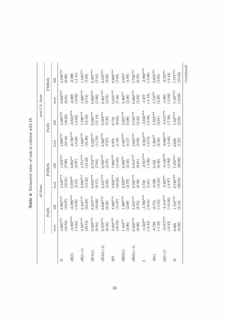
Table 4 presents the results of the models that include the dispersion of analysts’ forecasts
(dispM ) and its interaction with cash. Again, the estimation is carried out for the whole
29

sample as well as for the sample without U.S. firms. The observations for which dispM is not
defined drop away. The numbers of groups stay the same because in a first step we exclude
all firms for which dispM is not defined in at least one year. In all specifications we find a
significantly negative coefficient for the interaction variable. Apparently, the results clearly
support our Hypothesis 2 and not Hypothesis 1. That means that the value of cash is not
higher when the degree of IA is higher—it is even lower. Thus, the free cash flow problem
seems to be more relevant in relation to IA than the advantage of having a liquidity reserve
when raising external funds is difficult. To see whether the negative effect of IA on liquidity is
also economically significant, we calculate—despite our own reservations—the marginal value
of cash and the influence of IA. By including an interaction term in the analysis, the marginal
value of cash has to be calculated as follows:
V
A= α+ ...+ βc
C
A+ βINT
(C
A× dispM
)+ βdispMdispM (8)
∂ VA
∂ CA
=∂V
∂C= βc + βINT dispM (9)
30
Tab
le4:
Est
imat
edva
lue
ofca
shin
rela
tion
wit
hIA
all
firm
snon-U
.S.
firm
s
Fix
Ef.
FM
Bet
hF
ixE
f.F
MB
eth
level
diff
.le
vel
diff
.le
vel
diff
.le
vel
diff
.
E4.3
05***
3.9
83***
2.4
48***
1.8
72***
4.2
99***
4.2
06***
3.0
32***
3.1
06***
(18.9
4)
(12.9
7)
(12.3
1)
(7.9
0)
(10.1
8)
(10.2
0)
(6.6
1)
(6.9
9)
dE
(t)
-0.3
68***
-0.3
96***
0.7
89**
0.8
04**
-0.7
36***
-0.8
24***
-0.2
69
-0.3
99
(-3.0
4)
(-2.9
4)
(3.1
5)
(3.0
7)
(-3.3
9)
(-3.6
2)
(-0.9
2)
(-1.4
1)
dE
(t+
1)
2.4
87***
2.1
64***
2.3
39***
1.7
71***
1.9
48***
1.7
36***
1.3
66***
1.1
26***
(23.7
4)
(22.8
3)
(14.3
2)
(12.4
3)
(10.3
6)
(11.9
3)
(6.7
4)
(7.0
3)
dN
A(t
)0.3
29***
0.3
12***
0.8
19***
0.7
12***
0.2
28***
0.2
28***
0.6
00***
0.4
97***
(9.0
4)
(10.6
6)
(8.1
7)
(7.6
4)
(11.7
8)
(11.1
9)
(5.9
0)
(5.2
4)
dN
A(t
+1)
0.5
79***
0.6
46***
0.4
47***
0.5
58***
0.5
68***
0.5
83***
0.4
61***
0.5
10***
(6.8
4)
(8.5
6)
(4.0
5)
(4.7
8)
(7.0
7)
(7.4
9)
(3.7
2)
(3.8
9)
RD
5.0
22***
4.2
80***
5.8
33***
7.6
60***
0.9
79
0.7
18
5.6
55***
6.6
02***
(19.1
9)
(11.8
7)
(10.2
4)
(11.8
4)
(1.1
8)
(0.8
2)
(7.4
0)
(7.6
5)
dR
D(t
)1.1
04**
1.2
96***
2.1
95**
2.4
96**
2.4
05***
2.2
81***
3.4
69**
3.0
15*
(2.0
6)
(2.6
9)
(2.7
9)
(2.4
2)
(4.1
7)
(4.0
0)
(2.4
6)
(1.9
9)
dR
D(t
+1)
6.5
68***
5.4
54***
8.7
00***
9.4
54***
3.0
25***
2.7
36***
6.9
60***
7.7
36***
(8.9
0)
(9.7
4)
(8.3
9)
(8.6
1)
(3.5
9)
(3.4
2)
(5.9
3)
(6.7
8)
I-1
.318**
-1.7
06***
0.7
38
-2.8
57***
-2.5
64***
-2.8
36***
-1.0
77
-2.9
92***
(-2.4
4)
(-2.6
4)
(1.0
1)
(-4.2
6)
(-4.7
4)
(-5.5
8)
(-1.1
8)
(-3.9
8)
dI(
t)-0
.728
-0.7
74
-0.5
90
0.4
22
1.2
84**
1.2
53***
1.7
19**
2.6
73***
(-1.5
6)
(-1.5
3)
(-0.4
4)
(0.4
8)
(2.4
6)
(2.6
1)
(2.2
8)
(4.0
1)
dI(
t+1)
-3.5
71***
-4.4
13***
-2.9
97**
-5.1
26***
-2.6
06***
-3.1
47***
-1.0
85
-2.2
37**
(-9.3
5)
(-12.2
0)
(-2.9
7)
(-5.0
2)
(-5.8
2)
(-7.5
0)
(-1.0
2)
(-2.4
3)
D0.0
88
1.1
52***
6.7
40***
7.4
70***
0.6
29
1.3
37***
7.1
97***
7.7
77***
(0.2
0)
(3.1
3)
(20.9
4)
(20.6
9)
(1.2
5)
(2.9
3)
(12.0
6)
(15.5
3)
(continued
)
31

Tab
le4:
—co
ntin
ued
all
firm
snon-U
.S.
firm
s
Fix
Ef.
(lev
el/diff
.)F
MB
eth
(lev
el/diff
.)F
ixE
f.(l
evel
/diff
.)F
MB
eth
(lev
el/diff
.)
dD
(t)
-0.3
24
-0.3
67*
-2.4
78***
-1.8
53***
-0.2
99
-0.3
49
-1.9
45***
-1.6
73***
(-1.3
7)
(-1.7
8)
(-5.1
3)
(-3.7
7)
(-0.9
8)
(-1.1
3)
(-4.8
2)
(-3.8
6)
dD
(t+
1)
0.1
02
0.5
71***
2.4
83***
3.3
93***
0.2
01
0.4
94
2.7
63***
3.2
63***
(0.5
5)
(3.0
4)
(7.5
0)
(8.6
5)
(0.6
2)
(1.6
3)
(5.2
5)
(6.1
2)
dV
(t+
1)
-0.2
72***
-0.3
05***
-0.1
42
-0.1
78
-0.2
80***
-0.2
98***
-0.1
86
-0.2
09
(-5.6
6)
(-6.0
9)
(-1.4
4)
(-1.6
2)
(-4.6
4)
(-4.8
6)
(-1.3
5)
(-1.4
6)
dis
pM
0.0
09
-0.0
62***
-0.0
33
-0.0
52
0.0
36
-0.0
63***
0.1
79***
0.1
60**
(0.4
2)
(-4.7
1)
(-1.0
0)
(-1.2
7)
(1.2
8)
(-3.2
1)
(3.7
7)
(3.0
1)
C0.7
82***
2.1
18***
0.3
91***
1.3
08***
(4.5
0)
(10.8
4)
(4.5
3)
(6.4
8)
dC
(t)
1.0
07***
2.0
50***
0.6
95***
1.4
36***
(12.0
3)
(6.0
8)
(7.6
1)
(4.7
8)
dC
(t+
1)
1.0
09***
1.2
20***
0.8
03***
0.8
47***
(6.8
8)
(4.6
0)
(6.8
7)
(3.9
5)
C×
dis
pM
-0.5
94***
-0.3
26*
-1.0
41***
-0.5
12**
(-3.3
4)
(-1.9
6)
(-10.2
4)
(-2.4
5)
dC
(t+
1)×
dis
pM
-1.1
49***
-3.4
00***
-0.8
85***
-2.5
44***
(-5.9
9)
(-6.1
2)
(-6.5
2)
(-4.3
0)
Const
.0.9
25***
1.0
16***
0.5
35***
0.8
15***
0.7
51***
0.9
45***
0.4
94***
0.6
29***
(21.5
1)
(45.2
4)
(29.2
1)
(36.8
1)
(21.9
3)
(36.4
7)
(24.9
2)
(27.2
1)
R2
0.3
46
0.3
76
0.4
33
0.4
09
0.3
34
0.3
51
0.4
26
0.4
24
N29963
29708
29963
29708
19661
19585
19661
19585
Gro
ups
7474
7412
10
10
4991
4970
10
10
Est
imati
on
resu
lts
wit
hIA
for
fixed
effec
tsre
gre
ssio
ns
(Fix
Ef.
)an
dF
am
aM
acB
eth
regre
ssio
ns
(FM
Bet
h)
over
the
1995
to2005
per
iod
.T
he
dep
end
ent
vari
ab
lein
all
spec
ifica
tion
sis
the
tota
lm
ark
etvalu
esc
ale
dby
tota
lass
ets.
Defi
nit
ion
sof
all
vari
ab
les
are
pro
vid
edin
Sec
tion
3.1
.2.
Yea
rd
um
mie
sare
incl
ud
ed,
bu
tare
not
pre
sente
d.
Sta
tist
ical
infe
ren
ceis
base
don
Dri
scoll
an
dK
raay
(1998).
t-valu
esare
pre
sente
din
pare
nth
eses
.T
he
R2
of
the
fixed
effec
tsre
gre
ssio
nre
pre
sents
the
R2
of
the
wit
hin
dim
ensi
on.
***,
**
an
d*
ind
icate
sign
ifica
nce
at
the
1%
,5%
,an
d10%
level
,re
spec
tivel
y.
32

Considering the results of the fixed effects estimation with the cash level, the coefficient of C
is 0.782 and that of the interaction is -0.594. Based on the median value of dispM (0.109, see
Table 2) the marginal value of cash is 0.717. An increase in the degree of IA of one standard
deviation (0.249, see Table 2) results in a marginal value of cash that is 0.148 units of money
lower, i.e., the marginal value amounts to 0.569. We conclude that the negative effect of IA
on cash is substantial. To control for the direct influence of the dispersion on the firm value,
we also included the variable dispM by itself. We did not formulate an explicit expectation
on the coefficient of this variable. The results reveal that there is no clear relationship. In
some specifications it is negative; in others it is positive. The negative relationship can be
explained by the fact that IA in general is something unfavorable. Another explanation could
be based on a possible correlation with a firm’s risk. A possible reason for a positive result
could be related to the model of Miller (1977). He argues that under certain assumptions a
higher divergence of opinions among investors tends to increase the market value of securities
as only the most optimistic investors engage in trading.19
In Table 5 we present the results of our more detailed analysis by splitting the sample according
to firm characteristics. First, we examine splits by the firm size (measured with market
capitalization) and by the payout ratio to test the impact of financial constraints. Second,
the sample is split by the proportion of inside ownership (closely held shares) to test for an
influence of the corporate governance structure. Considering the results of the fixed effects
estimation, we can conclude that cash has a higher value for small firms (smaller than the
median firm) than for large firms (larger than the median firm). This is consistent with the
idea that large firms can more easily access financial markets, but the result is not robust.
The estimation with the Fama-MacBeth method does not confirm this finding, but that does
not pose a problem as we are primarily interested in the coefficient of the interaction term,
for which we are able to present more robust results. The negative effect of IA on cash is less
strong (or does not even exist) for small firms. Supposedly, the negative effect of IA on cash
(as predicted by Hypothesis 2) is to some extent canceled out by an opposite effect, i.e., cash
is more important in periods with higher IA (as predicted by Hypothesis 1). When the payout
19 Diether et al. (2002) provide evidence for this model.
33

ratio is used as a proxy for the degree of financial constraints, we again find that cash is more
valuable for firms that face financing constraints. The results for the interaction variable are
mixed. Based on the split by the payout ratio we cannot conclude that there is an opposite
effect as discussed before. The final split by firm characteristics results in three groups. In
the choice of the cut-off levels (0–5%, 5–25%, and 25% or more) we follow Morck et al. (1988)
(see also Opler et al., 1999, for these cut-off levels). Thus, we expect that cash has less value
and that IA has a more negative impact for firms with inside ownership between 5% and 25%
due to an entrenchment effect. Firms with such a high proportion of managerial ownership
could suffer more from agency conflicts because the managers could fleece the shareholders
more easily. Yet, in most specifications we find that cash has a higher value in the middle
range, contrary to the prediction. Thus, the findings indicate that in the middle range an
incentive effect is prevalent rather than an entrenchment effect and it is in line with the
results of McConnell and Servaes (1990). They find a positive relationship between firm value
and inside ownership up to a fraction of about 45%. The relationship between the coefficient
of the interaction variable and the proportion of the closely held shares is not that clear. We
can only detect a tendency that the negative influence of IA is most pronounced for firms
featuring a low managerial shareholding.
Table 5: Estimated value of cash in different subgroups (firm characteristics)
all firms non-U.S. firms U.S. firms
FixEf. FMBeth FixEf. FMBeth FixEf. FMBeth
large C 0.467*** 2.249*** 0.176 1.454*** 1.114*** 3.647***firms (2.68) (8.47) (1.63) (5.62) (3.35) (9.33)
C×dispM -1.018*** -0.524 -1.307*** -1.539* 0.423 2.181*(-4.32) (-0.58) (-4.38) (-2.04) (1.10) (2.04)
N 14979 14979 10432 10432 4547 4547
Groups 3761 10 2760 10 1007 10
small C 0.844*** 1.919*** 0.335** 1.088*** 1.167*** 2.117***firms (4.08) (9.38) (2.18) (6.32) (4.50) (9.88)
C×dispM -0.281 -0.166 -0.463*** 0.175 0.041 -0.033(-1.20) (-0.41) (-3.49) (0.54) (0.13) (-0.08)
N 14984 14984 9229 9229 5755 5755
(continued)
34

Table 5: —continued
all firms non-U.S. firms U.S. firms
FixEf. FMBeth FixEf. FMBeth FixEf. FMBeth
Groups 4720 10 2799 10 1926 10
payout C 0.241 0.820*** 0.173 0.730*** 0.219 1.016***ratio high (1.39) (4.96) (1.10) (5.41) (0.78) (4.06)
C×dispM -0.250 -1.631** -0.299* -1.299** 0.904*** -1.353**(-0.79) (-2.58) (-1.73) (-2.42) (3.13) (-2.72)
N 14862 14862 11095 11095 3767 3767
Groups 4434 10 3322 10 1114 10
payout C 1.145*** 2.780*** 0.770*** 1.969*** 1.416*** 3.016***ratio low (4.75) (10.36) (3.41) (5.80) (5.37) (11.04)
C×dispM -0.658*** -1.036*** -1.367*** -1.280*** 0.062 -0.350(-2.82) (-5.93) (-5.83) (-4.73) (0.24) (-1.12)
N 14867 14867 8372 8372 6495 6495
Groups 5524 10 3374 10 2156 10
inside C 0.990*** 2.247*** 0.529* 1.078* 1.308*** 2.669***ownership (5.41) (6.09) (1.80) (1.84) (5.59) (7.78)
0-5% C×dispM -1.251** 0.322 -3.038*** 0.489 -1.212* -0.369(-2.45) (0.27) (-5.21) (0.25) (-1.73) (-0.33)
N 3326 3326 966 966 2360 2360
Groups 1144 10 410 10 734 10
inside C 1.042*** 2.671*** -0.061 1.351** 1.463*** 2.924***ownership (4.26) (9.79) (-0.29) (3.20) (4.83) (9.25)
5-25% C×dispM -0.501** 0.621 -1.899*** 1.276 0.105 0.742(-2.28) (1.15) (-3.37) (1.23) (0.49) (1.13)
N 6559 6559 2809 2809 3750 3750
Groups 2563 10 1175 10 1389 10
inside C 0.286*** 1.974*** 0.239** 1.092*** 0.600 2.842***ownership (2.61) (11.40) (2.15) (7.63) (1.53) (9.57)
+25% C×dispM -0.284 -0.851*** -0.911*** -1.438*** 0.436 -0.524(-1.14) (-3.67) (-4.20) (-3.25) (1.55) (-1.33)
N 14787 14787 10857 10857 3930 3930
Groups 4793 10 3260 10 1537 10
This table shows estimation results without IA for fixed effects regressions (FixEf.) and Fama-MacBeth regressions(FMBeth) for different sub-samples over the 1995 to 2005 period. The dependent variable in all specifications is the totalmarket value scaled by total assets. Year dummies and different variables on firm characteristics (as in Table 3 and 4)are included in all specifications, but are not presented for brevity reasons. The definitions of all variables are providedin Section 3.1.2. Statistical inference is based on Driscoll and Kraay (1998). t-values are presented in parentheses. . ***,** and * indicate significance at the 1%, 5%, and 10% level, respectively.
35

We now turn to the estimation results included in Table 6 where we split the sample by proxies
for the corporate governance and financing practices at the country level. The first three splits
are based on three indices that were described in Section 3.1.3, i.e., the rule of law index, the
anti-director-rights index and the corruption index. For each index, the sample is divided
into two groups according to a higher (lower) index value than the median country. A higher
index value indicates that a country has better corporate governance practices. With very
few exceptions we find exactly what we expected. The coefficient of cash is higher (with one
exception) for firms located in countries with a higher index value and the negative influence of
IA on cash is stronger for firms in countries with a lower index value (also with one exception).
This result supports the idea that IA is more problematic for firms operating in countries with
lower corporate governance standards.
The next two splits are based on the financing practices of the countries. We use the stock
market capitalization and that of the private bond market, respectively, divided by the gross
domestic product as measurement for the financing practices. We expect that in countries with
a lower level of those ratios, internal financing is more important and hence cash holdings play
a major role. If we were to find a less negative coefficient of the interaction term or even a
positive relationship between cash and IA, we would interpret this result as supporting our
Hypothesis 1. Surprisingly, we find exactly the opposite. The coefficient of cash and the
coefficient of the interaction term are generally smaller for firms in countries with a lower
ratio. Therefore, we cannot corroborate our Hypothesis 1. We put forward two reasons for
this finding. The first explanation is based on the correlation of a country’s financing and its
corporate governance practices. Common law countries are typically market-based countries
and we can expect that these countries have a higher ratio of bond and stock capitalization to
GDP than civil law countries. At the same time, investors generally are better protected in
common law countries (La Porta et al., 2000). Our other explanation is based on the role of IA
in capital markets and the role of financial intermediaries. Civil law countries are rather bank-
based and, therefore, financial intermediaries play a decisive role. Financial intermediaries can
be considered as a natural response to IA (Leland and Pyle, 1977). In contrast to shareholders
and bondholders, banks know more about a company’s prospects because banks have more
36

information sources than the average market participant. Hence, the adverse selection problem
is less important for banks than for other investors. Consequently, in market-based countries
where firms typically access financial markets to raise funds, IA is more problematic. Thus,
our Hypothesis 1 (cash has more value when IA is high) should be more important for common
law countries and this could be reflected in the less negative interaction term, which is not
even significant in most specifications.
Table 6: Estimated value of cash in different subgroups (country characteristics)
all firms non-U.S. firms
FixEf. FMBeth FixEf. FMBeth
rule of C 0.883*** 2.427*** 0.426*** 1.481***law index high (4.92) (11.10) (4.97) (5.56)
C×dispM -0.497** -0.062 -0.998*** 0.016(-2.54) (-0.24) (-6.93) (0.05)
N 23240 23240 12938 12938
Groups 5470 10 2986 10
rule of C 0.374** 0.950*** 0.374** 0.950***law index low (2.34) (5.34) (2.34) (5.34)
C×dispM -1.281*** -1.674*** -1.281*** -1.674***(-4.62) (-3.50) (-4.62) (-3.50)
N 6723 6723 6723 6723
Groups 2011 10 2011 10
anti-director C 1.028*** 2.471*** 0.533*** 1.213***rights index high (4.99) (10.82) (6.12) (5.18)
C×dispM -0.269 0.055 -0.996*** -0.008(-1.14) (0.20) (-3.66) (-0.02)
N 17246 17246 6944 6944
Groups 4217 10 1726 10
anti-director C 0.250** 1.353*** 0.250** 1.353***rights index low (2.16) (4.79) (2.16) (4.79)
C×dispM -0.985*** -0.721* -0.985*** -0.721*(-5.26) (-1.95) (-5.26) (-1.95)
N 11966 11966 11966 11966
Groups 3048 10 3048 10
(continued)
37

Table 6: —continued
all firms non-U.S. firms
FixEf. FMBeth FixEf. FMBeth
corruption C 0.883*** 2.427*** 0.426*** 1.481***index high (4.92) (11.10) (4.97) (5.56)
C×dispM -0.497** -0.062 -0.998*** 0.016(-2.54) (-0.24) (-6.93) (0.05)
N 23240 23240 12938 12938
Groups 5470 10 2986 10
corruption C 0.374** 0.950*** 0.374** 0.950***index low (2.34) (5.34) (2.34) (5.34)
C×dispM -1.281*** -1.674*** -1.281*** -1.674***(-4.62) (-3.50) (-4.62) (-3.50)
N 6723 6723 6723 6723
Groups 2011 10 2011 10
stock/gdp C 0.852*** 2.357*** 0.378*** 1.452***high (4.57) (10.95) (3.54) (5.62)
C×dispM -0.436** -0.071 -0.861*** -0.017(-2.43) (-0.29) (-7.40) (-0.06)
N 24886 24886 14584 14584
Groups 5943 10 3458 10
stock/gdp C 0.373*** 1.034*** 0.373*** 1.034***low (6.90) (10.15) (6.90) (10.15)
C×dispM -1.378*** -1.338*** -1.378*** -1.338***(-5.59) (-3.82) (-5.59) (-3.82)
N 5077 5077 5077 5077
Groups 1539 10 1539 10
bond/gdp C 0.814*** 2.430*** 0.097 1.418***high (3.88) (11.45) (0.73) (4.87)
C×dispM -0.497** -0.276 -0.863*** -0.179(-2.48) (-1.54) (-5.01) (-0.50)
N 22494 22494 12192 12192
Groups 5528 10 3044 10
bond/gdp C 0.619*** 1.032*** 0.619*** 1.032***low (3.71) (5.36) (3.71) (5.36)
C×dispM -0.701*** -1.206* -0.701*** -1.206*(-2.67) (-2.12) (-2.67) (-2.12)
N 6995 6995 6995 6995
(continued)
38

Table 6: —continued
all firms non-U.S. firms
FixEf. FMBeth FixEf. FMBeth
Groups 1788 10 1788 10
common C 1.045*** 2.491*** 0.517*** 1.164***law (4.89) (10.60) (3.96) (4.69)
C×dispM -0.215 0.078 -0.859*** -0.053(-0.91) (0.27) (-3.05) (-0.13)
N 16008 16008 5706 5706
Groups 3981 10 1490 10
civil C 0.283*** 1.345*** 0.283*** 1.345***law (2.70) (5.28) (2.70) (5.28)
C×dispM -1.048*** -0.618* -1.048*** -0.618*(-6.94) (-2.02) (-6.94) (-2.02)
N 13955 13955 13955 13955
Groups 3506 10 3506 10
This table shows estimation results without IA for fixed effects regressions (FixEf.) and Fama-MacBeth regressions(FMBeth) for different sub-samples over the 1995 to 2005 period. The dependent variable in all specifications is the totalmarket value scaled by total assets. Year dummies and different variables on firm characteristics (as in Table 3 and 4)are included in all specifications, but are not presented for brevity reasons. The definitions of all variables are providedin Section 3.1.2. Statistical inference is based on Driscoll and Kraay (1998). t-values are presented in parentheses. . ***,** and * indicate significance at the 1%, 5%, and 10% level, respectively.
4.2 Results from the Approach by Dittmar and
Mahrt-Smith (2007)
In Table 7 we report the results from estimating the Fama and French (1998) valuation re-
gression for firms that experience a positive value of excess cash (refer to Section 3.2.2). The
results are estimated with fixed effects regressions (our standard model) and as a double check
we also run Fama-MacBeth regressions. In order to control for a U.S. effect, the results are
also shown without North American firms. The value for ExCash is statistically and econom-
ically significant. Specifically, the marginal value of excess cash is positive and significant
at the one percent level for all specifications. Focusing on the results from the fixed effects
estimator, the coefficient of ExCash amounts to 1.905 which means that one dollar put into
excess cash increases the firm value by more than its par value. These results point to a
value-enhancing role of excess cash and they are comparable to other studies in this field, e.g.,
39

Dittmar and Mahrt-Smith (2007) who find a value for excess cash of 2 to 3 dollars depending
on the governance proxy used.20
However, as outlined above the emphasis of our study is placed on investigating the value
consequences of cash in the presence of IA. Therefore, in Table 7 the models also include the
dispersion of analysts’ earnings forecasts (dispM ) as our measure for IA. In order to study the
combined effect of excess cash and IA, an interaction variable is also included in the model.
Our results reveal that the coefficient on the interaction term is negative and significant in all
but one specification. Importantly, we find that IA decreases the marginal benefit of holding
excess cash. This means that the empirical evidence corroborates our Hypothesis 2. In order to
illustrate the detrimental value effect of IA, we calculate the marginal value of excess cash with
IA for the fixed effects calculations (see Section 4.1). In Table 7 the stand-alone coefficient on
ExCash amounts to 1.905. However, if IA is taken into account, the marginal value of excess
cash is reduced to a value of 1.863 (based on a median value of dispM of 0.088 according to
Table 2 (Panel B).21 And if we now increase the IA by one standard deviation [0.241, see Table
2 (Panel B)], the marginal value of excess cash decreases by 0.115 (6.2%) money units to a
low level of 1.747.22 Therefore, these results can be interpreted as a valuation discount placed
on firms where IA constitutes a problem and the evidence clearly supports our Hypothesis 2.
This means that the agency costs from the free-cash flow theory dominate any supposed cost
savings from the availability of internal capital.
The empirical models presented thus far provided a first attempt to investigate whether IA
impacts the value effect of cash holdings. However, for the sake of distinguishing more accu-
rately between our two conflicting hypotheses, we split the sample into subgroups based on
corporate governance (related to the free cash flow theory) and financing constraints (related
20 Dittmar and Mahrt-Smith (2007) abstain from interpreting the stand-alone coefficient on excess cash asthey argue that excess cash could still be afflicted with endogeneity and hence they only focus on theinterpretation of their interaction term (excess cash times governance index).
21 The calculation is done as follows: 1.905 + (−0.479) × 0.088. For more information on the calculation ofthe marginal value of cash, refer to Section 4.1.
22 The calculation is done as follows: 1.905 + (−0.479)× (0.088 + 0.241).
40

to Myers and Majluf (1984) adverse selection problem) (for details refer to 3.1.3).23
Table 7: Estimated value of excess cash in relation with IA
all firms non-U.S. firms
FixEf. FMBeth FixEf. FMBeth
E 5.440*** 2.337*** 5.223*** 3.207***(24.76) (5.47) (14.52) (5.34)
dE(t) -0.057 1.894*** -0.511* 0.17(-0.61) (5.18) (-1.68) (0.39)
dE(t+1) 3.281*** 2.681*** 2.089*** 0.858(12.91) (8.26) (4.58) (1.42)
dNA(t) 0.351*** 1.076*** 0.176*** 0.421***(2.74) (8.05) (3.49) (4.62)
dNA(t+1) 0.697*** 0.634*** 0.484*** 0.483**(6.13) (4.18) (3.70) (2.37)
RD 10.748*** 8.183*** 8.268*** 6.627***(6.56) (11.57) (3.52) (5.90)
dRD(t) -2.088 0.498 0.668 4.338(-1.46) (0.28) (0.59) (1.54)
dRD(t+1) 8.260*** 9.044*** 4.227** 7.444***(9.89) (4.80) (2.15) (5.47)
I -0.775 -4.560*** -2.846 -5.307***(-0.73) (-4.23) (-1.21) (-4.99)
dI(t) 0.586 -1.327 3.311*** 3.233***(0.71) (-0.65) (2.83) (3.51)
dI(t+1) -2.381*** -8.829*** -1.663 -3.851*(-3.49) (-6.51) (-1.55) (-2.09)
D -2.130*** 4.492*** 0.511 4.868***(-5.12) (10.51) (0.94) (7.14)
dD(t) -0.215 -2.553** -0.296 -1.787**(-0.76) (-2.89) (-0.71) (-3.21)
(continued)
23 The only difference to the classifications taken for the actual cash ratio is that in the case of excess cash weabstain from grouping firms along the dimension of size and the payout ratio as these two characteristicsare endogenously related to the computation of excess cash and the ownership split is also omitted as theresults have turned out to be not significant for the actual cash ratio.
41

Table 7: —continued
all firms non-U.S. firms
FixEf. FMBeth FixEf. FMBeth
dD(t+1) -1.169*** 0.781 0.159 1.294(-8.78) (1.06) (1.07) (1.67)
dV(t+1) -0.274*** -0.136 -0.154* -0.048(-4.09) (-1.26) (-1.78) (-0.29)
dispM -0.007 -0.034 0.04 0.131(-0.16) (-0.29) (0.66) (1.29)
ExCash 1.905*** 3.083*** 1.299*** 2.036***(8.84) (14.82) (7.41) (9.78)
ExCash×dispM -0.479** -0.42 -0.776*** -1.016**(-2.23) (-0.49) (-2.80) (-2.35)
Const. 1.182*** 1.063*** 0.948*** 1.019***(14.83) (21.59) (19.28) (28.36)
R2 0.444 0.589 0.362 0.617
N 10876 10876 6569 6569
Groups 3455 10 1895 10
Fixed effects regressions (with year dummies) and Fama-MacBeth regressions (1995 to 2005). The dependent variable isthe total market value scaled by net assets. The explanatory variables are defined in Section 3.1.3. T -values (Driscoll andKraay, 1998) are presented in parentheses. ***, ** and * indicate significance at the 1%, 5%, and 10% level, respectively.
The results are reported in Table 8. Accordingly, the first corporate governance grouping is
based on the rule of law index (corporate governance variable at the country level). A first
glimpse at the results reveals that they correspond to our expectations. The evidence for
the interaction term further confirms our Hypothesis 2 as the interaction term is significantly
more negative in low rule of law countries. This means that IA significantly decreases the
value of cash and this effect is even more pronounced if the governance environment is weak.
Moreover, this result is further emphasized by investigating the evidence for the anti-director-
rights index, which is a further corporate governance split at the country level. In line with
the previous discussion, the marginal value of excess cash is significantly decreased if the
shareholder protection is weak. Accordingly, this result further enforces Jensen’s (1986) free
cash flow theory. The evidence for the corruption index also points in the same direction.
The interaction term for high corruption countries (low corruption index) is negative and
relatively higher in absolute terms (-2.563) than the interaction term if corruption is relatively
low (-0.283). This means that a) IA decreases the value of cash and b) that this effect is
42

even more pronounced if the external governance environment is weak. The last split of
governance at the country-level (common law countries versus civil law countries) reveals that
according to expectations the coefficient on ExCash is lower in civil law countries (0.934)
versus common law countries. This confirms the results by La Porta et al. (1998) indicating
that the governance environment in countries with a civil law tradition is weaker. This result
is also confirmed by the interaction term, which is significantly negative in civil-law countries
and not significant, albeit still negative, in common-law countries. Taken together, the splits
according to corporate governance measures further emphasize that the free cash flow theory
of Jensen (1986) is the common denominator between the results because the coefficient on
ExCash is lower in a low governance environment as well as the interaction being more negative
if the governance is weaker.
Table 8: Estimated value of cash in different subgroups (country characteristics)
all firms non-U.S. firms
FixEf. FMBeth FixEf. FMBeth
rule of ExCash 1.952*** 3.172*** 1.165*** 2.164***law index high (6.59) (12.55) (5.82) (7.76)
ExCash×dispM -0.317* 0.194 -0.258 -1.175*(-1.70) (0.16) (-0.89) (-1.89)
N 8513 8513 4206 4206
Groups 2768 10 1207 10
rule of ExCash 1.403*** 1.738*** 1.403*** 1.738***law index low (5.68) (5.77) (5.68) (5.77)
ExCash×dispM -1.982*** -0.112 -1.982*** -0.112(-5.28) (-0.10) (-5.28) (-0.10)
N 2363 2363 2363 2363
Groups 688 10 688 10
(continued)
43

Table 8: —continued
all firms non-U.S. firms
FixEf. FMBeth FixEf. FMBeth
anti-director ExCash 2.155*** 3.370*** 1.948*** 2.435***rights index high (6.17) (13.27) (6.76) (6.29)
ExCash×dispM -0.26 0.051 -1.241 -0.552(-1.15) (0.04) (-1.51) (-0.42)
N 6578 6578 2271 2271
Groups 2288 10 723 10
anti-director ExCash 0.929*** 1.884*** 0.929*** 1.884***rights index low (7.56) (8.93) (7.56) (8.93)
ExCash×dispM -0.446** -1.478** -0.446** -1.478**(-2.27) (-2.71) (-2.27) (-2.71)
N 4295 4295 4295 4295
Groups 1170 10 1170 10
corruption ExCash 1.929*** 3.180*** 0.977*** 2.078***index high (6.34) (12.71) (5.70) (8.28)
ExCash×dispM -0.283 0.193 -0.034 -0.941(-1.45) (0.16) (-0.11) (-1.49)
N 8442 8442 4135 4135
Groups 2769 10 1208 10
corruption ExCash 1.802*** 1.895*** 1.802*** 1.895***index low (4.42) (5.72) (4.42) (5.72)
ExCash×dispM -2.563*** -0.367 -2.563*** -0.367(-5.54) (-0.36) (-5.54) (-0.36)
N 2434 2434 2434 2434
Groups 689 10 689 10
stock/gdp ExCash 1.948*** 3.170*** 1.041*** 2.086***high (7.48) (13.26) (9.35) (12.44)
ExCash×dispM -0.329 0.115 -0.457 -0.181(-1.41) (0.11) (-1.51) (-0.29)
N 8738 8738 4431 4431
Groups 2819 10 1258 10
stock/gdp ExCash 1.643*** 1.975*** 1.643*** 1.975***low (3.67) (3.88) (3.67) (3.88)
ExCash×dispM -1.912** -2.910* -1.912** -2.910*(-2.27) (-2.11) (-2.27) (-2.11)
N 2138 2138 2138 2138
Groups 639 10 639 10
(continued)
44

Table 8: —continued
all firms non-U.S. firms
FixEf. FMBeth FixEf. FMBeth
bond/gdp ExCash 1.861*** 3.138*** 0.748*** 1.769***
high (6.71) (13.84) (8.19) (8.67)
ExCash×dispM -0.325 -0.171 -0.291 -1.164*(-1.26) (-0.18) (-1.37) (-2.05)
N 8285 8285 3978 3978
Groups 2623 10 1061 10
bond/gdp ExCash 1.847*** 2.199*** 1.847*** 2.199***low (5.80) (5.84) (5.80) (5.84)
ExCash×dispM -1.194* 0.063 -1.194* 0.063(-1.67) (0.06) (-1.67) (0.06)
N 2454 2454 2454 2454
Groups 787 10 787 10
common ExCash 2.157*** 3.344*** 1.934*** 2.525***law (6.00) (13.11) (6.11) (6.24)
ExCash×dispM -0.197 0.155 -0.986 -1.251(-0.88) (0.11) (-1.11) (-0.92)
N 6256 6256 1949 1949
Groups 2191 10 626 10
civil ExCash 0.934*** 1.910*** 0.934*** 1.910***law (7.79) (8.95) (7.79) (8.95)
ExCash×dispM -0.492** -1.476** -0.492** -1.476**(-2.55) (-2.69) (-2.55) (-2.69)
N 4620 4620 4620 4620
Groups 1269 10 1269 10
This table shows estimation results without IA for fixed effects regressions (FixEf.) and Fama-MacBeth regressions(FMBeth) for different sub-samples over the 1995 to 2005 period. The dependent variable in all specifications is the totalmarket value scaled by total assets. Year dummies and different variables on firm characteristics (as in Table 3 and 4)are included in all specifications, but are not presented for brevity reasons. The definitions of all variables are providedin Section 3.1.2. Statistical inference is based on Driscoll and Kraay (1998). T -values are presented in parentheses. .***, ** and * indicate significance at the 1%, 5%, and 10% level, respectively.
Finally, the results for the splits according to financing constraints at the country-level
(stock/gdp and bond/gdp) should proxy for the fact that in countries where the capital mar-
ket is less developed, i.e., lower stock/gdp and/or lower bond/gdp, hoarding cash becomes
more important as external finance is harder to obtain. This means that we expect that in
countries where the capital market development is lower, the coefficient on ExCash is higher
and the interaction term is relatively less negative. However, this prediction is not borne out
45

by our data. For both measures of the capital market development (stock/gdp and bond/gdp)
the coefficient on ExCash is lower for more constrained countries and the interaction term is
only significantly negative in the same environment. One explanation of this result is that our
proxy for the capital market development is imperfect as there is a high correlation between
the country law tradition (civil law versus common law) and our capital market development
measures. In effect, stock/gdp and bond/gdp are then actually proxies for the governance
environment and hence, to a lesser extent, measures for the capital market development.
In a nutshell, the results provide an overwhelming view that IA decreases the value of cash,
which is in line with Jensen’s (1986) free cash flow argument and which corresponds to our
Hypothesis 2. On the other hand, the results consequently do not confirm Myers and Majluf’s
(1984) argumentation for the value benefits of financial slack (our Hypothesis 1).
4.3 Robustness Tests
To further test the robustness of our main result, we alter the specification of our estimations
as well as the definition of some variables. The coefficients of interest are presented in Table 9.
For brevity, we only report (with one exception) the results of the fixed effects estimation with
the level of cash. For the ease of comparison, Panel A of Table 9 shows again the coefficients
of cash and the interaction variable as they were presented in the first column of Table 4. The
other panels show the results of the robustness tests where we changed some parameters of
the estimations as described subsequently:
• Panel B: As discussed above, the valuation regression used in this study is based on
Fama and French (1998). While they use two-year changes for the calculation of those
explanatory variables that capture differences, we followed in our main specification
Pinkowitz et al. (2006) and Dittmar and Mahrt-Smith (2007) who only use one-year
changes. By using two-year changes the sample becomes smaller, but we still find a
clear negative influence of IA on the value of cash.
46

• Panel C: We estimate the regression without including time dummies. The coefficients
and the statistical inference do not change considerably.
• Panel D: In this specification we estimated the model with ordinary least squares and
cluster robust standard errors (Arellano (1987), Rogers (1993)). The coefficient of C
changes considerably, that of the interaction variable changes to a lesser extent. The
interaction remains significant but not anymore at the 1% significance level.
• Panel E: To control for a possible correlation between risk and IA we include two more
variables. First, we add the volatility of the monthly stock returns over the year. Second,
we include the interaction of the volatility and the cash ratio (C ). We find a higher coef-
ficient and a higher t-value for the interaction of cash and IA. Moreover, the estimation
reveals that there is a positive interaction between cash and risk (at least for non-U.S.
firms). This can be explained by the fact that cash is more important when the risk of
the firm is higher. This test indicates that the influence of risk and of the IA runs in
the opposite direction. Obviously, we can conclude that our results cannot be explained
by a positive correlation between our measurement of IA and risk.
• Panel F: In Panel F, we change the proxy for IA. Instead of using the dispersion of
analysts’ forecasts, we employ the forecast error (see the discussion in Section 3.1.1).
We calculate this variable as follows:
forecastError = ln(
1 +|epsforecast − epsactual|
|median|
)(10)
where the forecast of the earnings per share is the average of all forecasts provided by
the analysts in November and December. The difference of the actual and the forecasted
earnings per share in absolute terms is scaled by the median of the earnings per share
forecast. Similar to the calculation of dispM, we add one to this ratio and take the
natural logarithm. Observations are excluded if the average of the forecasts is not at
least based on the estimates of two analysts. The estimation indicates that our main
finding is robust to a change of the measurement of IA.
47

Table 9: Robustness tests
all firms non-U.S. firms
Panel A C 0.782*** 0.391***(base case) (4.50) (4.53)
C×dispM -0.594*** -1.041***(-3.34) (-10.24)
N 29963 19661
Groups 7474 4991
Panel B C 0.512** 0.296**(2-year lags) (2.22) (2.05)
C×dispM -0.804*** -0.754***(-4.15) (-9.51)
N 22908 15182
Groups 6072 4135
Panel C C 0.839*** 0.566***(no time dummies) (4.65) (6.54)
C×dispM -0.587*** -1.163***(-2.97) (-9.17)
N 29963 19661
Groups 7474 4991
Panel D C 2.281*** 1.501***(pooled OLS) (19.28) (10.79)
C×dispM -0.610** -0.479*(-2.31) (-1.83)
N 29963 19661
Groups 7474 4991
Panel E C 0.567** 0.215*(volatility) (2.34) (1.73)
C×dispM -0.687*** -1.205***(-3.72) (-14.97)
Vola -0.322** -0.129(1.98) (0.79)
C×Vola 1.534 1.730**(1.58) (2.00)
N 29559 19441
Groups 7408 4961
(continued)
48

Table 9: —continued
all firms non-U.S. firms
Panel F C 0.797*** 0.266**(forecast error) (4.85) (2.54)
C×forecastError -0.237** -0.266***(-2.06) (-2.43)
N 31370 20452
Groups 8016 5354
This table provides an overview of the estimation results of different robustness tests. The sample period correspondsto the period from 1995 to 2005. The regression specifications are explained in Section 4.3. The dependent variable inall specifications is the total market value scaled by total assets. The definitions of all variables are provided in Section3.1.3 and Section 4.3, respectively. Statistical inference is based on Driscoll and Kraay (1998) (Panel A, B, C, E,F) andon White (1980) (Panel D). t-values are presented in parentheses. ***, ** and * indicate significance at the 1%, 5%, and10% level, respectively.
5 Conclusions
This paper examines the value effects of corporate cash holdings. To date, the common practice
in the cash holdings literature is to examine the valuation effects of cash holdings whereby
the researcher discriminates according to corporate governance measures. However, we take a
different perspective and focus on the valuation effects of cash in connection with information
asymmetry. Specifically, we put forward two different hypotheses. First, focusing on Myers
and Majluf (1984), cash in combination with information asymmetry should have a positive
influence on the value of the firm because the adverse selection problem will be mitigated.
Second, referring to Jensen (1986), the free cash flow argument coupled with information
asymmetry leads to moral hazard and accordingly the value of cash should be lower.
For the sake of empirically contrasting these two hypotheses, we employ a large data set cov-
ering 7,474 firms from 45 countries. We use the Fama and French (1998) valuation regressions
and derive our results from two different cash specifications. As the main approach we use the
actual cash ratio in line with Pinkowitz et al. (2006) and as a robustness test we also calculate
excess cash based on Opler et al. (1999) and Dittmar and Mahrt-Smith (2007).
The results for the actual cash ratio reveal that the value of one unit of cash without taking
49

information asymmetry into account is on average around one. This result is consistent with
previous papers in this field (see Pinkowitz and Williamson, 2004; Pinkowitz et al., 2006).
However, if a firm faces a high level of information asymmetry, the value of its cash reserves
is significantly and substantially reduced. This evidence indicates that the agency costs of the
free cash flow argument outweigh the benefits from cash as internal capital. For being able
to further distinguish between our two opposing hypotheses, we split the sample according
to governance and financing constraints. Taken together, these splits further emphasize our
results that agency costs due to moral hazard decrease the value of cash. Specifically, the
value of cash is higher if the level of governance is stronger. According to the splits on the
basis of financing constraints, the expectation that cash is valued relatively higher if the firms
are financially constrained (either on the firm-level or because the markets are less developed)
are only borne out partly by our data.
Our second approach which is based on the framework of Dittmar and Mahrt-Smith (2007)
and the calculation of excess cash according to Opler et al. (1999) serves as a robustness test
for the results above. If we use excess cash as our measure of cash holdings the results stay
qualitatively the same compared to the results derived with the actual cash ratio. Accordingly,
information asymmetry significantly decreases the value of excess cash. This evidence further
confirms the free cash flow theory by Jensen (1986) and provides no empirical justification
for the theoretical argument by Myers and Majluf (1984). When we consider the governance
and financing constraints in our second approach, the results are also in line with what was
found by the estimations with the actual cash ratio. Again the value of excess cash is higher
if the level of governance is stronger; however, based on financing constraints no clear picture
emerges.
Taken together, our comprehensive results—which survive extensive robustness tests—clearly
indicate that the agency costs from the free cash flow theory outweigh the benefits from
‘financial slack’ in mitigating adverse selection.
50

Appendix
Detailed formula for measure of information asymmetry (dispMi,t)
ln
1 +1
Mi,t×
√√√√√√ Mi,t∑mi,t=1
1Ami,t
−1 ×∑Ami,t
ami,t=1(EPSami,t
− 1Ami,t
×∑Ami,t
ami,t=1EPSami,t
)2
Medmi,t
with:
Medmi,t: Absolute median earning per share forecast in month m in year t for firm i
Ami,t: Number of analysts that cover firm i in year t in month m
Mi,t: Number of months for which more than three analysts cover firm i in year t
EPSami,t: Earnings per share estimate of analyst a for firm i in year t in month m
51

References
Almeida, H., M. Campello, and M. S. Weisbach (2004): “The Cash Flow Sensitivity ofCash,” Journal of Finance, 59, 1777–1804.
Arellano, M. (1987): “Computing Robust Standard Errors for Within-Groups Estimators,”Oxford Bulletin of Economics and Statistics, 49, 431–34.
Autore, D. and T. Kovacs (2005): “The Pecking Order Theory and Time-Varying AdverseSelection Costs,” Working paper, Virginia Tech, Department of Finance.
——— (2006): “Temporal Variation in Analyst Agreement and Financing Decisions,” Workingpaper, Available at SSRN: http://ssrn.com/abstract=639363.
Choe, H., R. W. Masulis, and V. K. Nanda (1993): “Common Stock Offerings Acrossthe Business Cycle: Theory and Evidence,” Journal of Empirical Finance, 1, 3–31.
Diether, K. B., C. J. Malloy, and A. Scherbina (2002): “Differences of Opinion andthe Cross Section of Stock Returns,” Journal of Finance, 57, 2113–2141.
Dittmar, A. and J. Mahrt-Smith (2007): “Corporate Governance and the Value of CashHoldings,” Journal of Financial Economics, 83, 599–634.
Dittmar, A., J. Mahrt-Smith, and H. Servaes (2003): “International corporate gov-ernance and corporate cash holdings,” Journal of Financial and Quantitative Analysis, 38,111–133.
D’Mello, R. and S. Ferris (2000): “The Information Effects of Analyst Activity as theAnnouncement of New Equity Issues,” Financial Management, 29, 78–95.
Driscoll, J. C. and A. C. Kraay (1998): “Consistent Covariance Matrix Estimation withSpatially Dependent Panel Data,” Review of Economics and Statistics, 80, 549–560.
Elton, E. J., M. J. Gruber, and M. N. Gultekin (1984): “Professional Expectations:Accuracy and Diagnosis of Errors,” Journal of Financial and Quantitative Analysis, 19, 351–363.
Fama, E. F. and K. R. French (1998): “Taxes, Financing Decisions, and Firm Value,”Journal of Finance, 53, 819–843.
Fama, E. F. and M. C. Jensen (1983): “Separation of Ownership and Control,” Journalof Law and Economics, 26, 301–325.
Fama, E. F. and J. D. MacBeth (1973): “Risk, Return, and Equilibrium: EmpiricalTests,” Journal of Political Economy, 81, 607–636.
Faulkeneder, M. and R. Wang (2006): “Corporate Financial Policy and the Value ofCash,” Journal of Finance, 61, 1957–1990.
52

Frank, M. and V. Goyal (2003): “Testing the pecking order theory of capital structure,”Journal of Financial Economics, 67, 217–248.
Hochle, D. (2007): “Robust standard errors for panel data sets with cross-sectional depen-dence,” Stata Journal, 7, 281–312.
Jensen, M. C. (1986): “Agency Costs of Free Cash Flow, Corporate Finance, and Takeovers,”American Economic Review, 76, 323–330.
Kalcheva, I. and K. V. Lins (2006): “International Evidence on Cash Holdings and Ex-pected Managerial Agency Problems,” ECGI - Finance Working Paper, Available at SSRN:http://ssrn.com/abstract=477241.
Keynes, J. M. (1936): The general theory of employment, interest and money, Macmillanfor the Royal Economic Society: London.
Korajczyk, R. A., D. J. Lucas, and R. L. McDonald (1992): “Equity Issues withTime-Varying Asymmetric Information,” Journal of Financial and Quantitative Analysis, 27,397–417.
Krishnaswami, S. and V. Subramaniam (1999): “Information asymmetry, valuation, andthe corporate spin-off decision,” Journal of Financial Economics, 53, 73–112.
La Porta, R., F. Lopez-de Silanes, A. Shleifer, and R. W. Vishny (1998): “Lawand Finance,” Journal of Political Economy, 106, 1113–1155.
——— (2000): “Investor protection and corporate governance,” Journal of Financial Eco-nomics, 58, 3–27.
Leary, M. T. and M. R. Roberts (2007): “The Pecking Order, Debt Capacity, andInformation Asymmetry,” Working paper.
Leland, H. E. and D. H. Pyle (1977): “Informational Asymmetries, Financial Structure,and Financial Intermediation,” Journal of Finance, 32, 371–387.
Lundstrum, L. (2003): “Firm value, information problems and the internal capital market,”Review of Quantitative Finance and Accounting, 21, 141–156.
McConnell, J. J. and H. Servaes (1990): “Additional evidence on equity ownership andequity value,” Journal of Financial Economics, 27, 595–612.
Miller, E. M. (1977): “Risk, Uncertainty, and Divergence of Opinion,” Journal of Finance,32, 1151–1168.
Miller, M. H. and D. Orr (1966): “A Model of the Demand for Money by Firms,”Quarterly Journal of Economics, 80, 413–435.
Morck, R., A. Shleifer, and R. Vishny (1988): “Management ownership and marketvaluation: An empirical analysis,” Journal of Financial Economics, 20, 293–315.
53
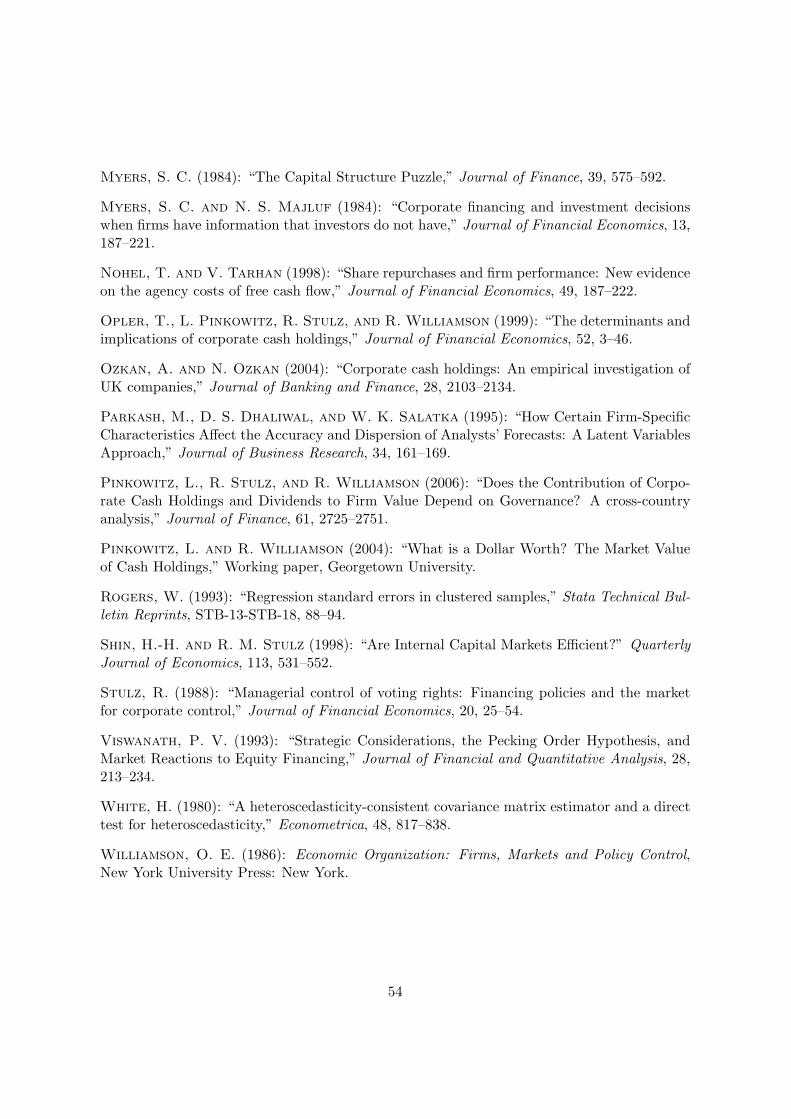
Myers, S. C. (1984): “The Capital Structure Puzzle,” Journal of Finance, 39, 575–592.
Myers, S. C. and N. S. Majluf (1984): “Corporate financing and investment decisionswhen firms have information that investors do not have,” Journal of Financial Economics, 13,187–221.
Nohel, T. and V. Tarhan (1998): “Share repurchases and firm performance: New evidenceon the agency costs of free cash flow,” Journal of Financial Economics, 49, 187–222.
Opler, T., L. Pinkowitz, R. Stulz, and R. Williamson (1999): “The determinants andimplications of corporate cash holdings,” Journal of Financial Economics, 52, 3–46.
Ozkan, A. and N. Ozkan (2004): “Corporate cash holdings: An empirical investigation ofUK companies,” Journal of Banking and Finance, 28, 2103–2134.
Parkash, M., D. S. Dhaliwal, and W. K. Salatka (1995): “How Certain Firm-SpecificCharacteristics Affect the Accuracy and Dispersion of Analysts’ Forecasts: A Latent VariablesApproach,” Journal of Business Research, 34, 161–169.
Pinkowitz, L., R. Stulz, and R. Williamson (2006): “Does the Contribution of Corpo-rate Cash Holdings and Dividends to Firm Value Depend on Governance? A cross-countryanalysis,” Journal of Finance, 61, 2725–2751.
Pinkowitz, L. and R. Williamson (2004): “What is a Dollar Worth? The Market Valueof Cash Holdings,” Working paper, Georgetown University.
Rogers, W. (1993): “Regression standard errors in clustered samples,” Stata Technical Bul-letin Reprints, STB-13-STB-18, 88–94.
Shin, H.-H. and R. M. Stulz (1998): “Are Internal Capital Markets Efficient?” QuarterlyJournal of Economics, 113, 531–552.
Stulz, R. (1988): “Managerial control of voting rights: Financing policies and the marketfor corporate control,” Journal of Financial Economics, 20, 25–54.
Viswanath, P. V. (1993): “Strategic Considerations, the Pecking Order Hypothesis, andMarket Reactions to Equity Financing,” Journal of Financial and Quantitative Analysis, 28,213–234.
White, H. (1980): “A heteroscedasticity-consistent covariance matrix estimator and a directtest for heteroscedasticity,” Econometrica, 48, 817–838.
Williamson, O. E. (1986): Economic Organization: Firms, Markets and Policy Control,New York University Press: New York.
54