INFORMATION ASYMMETRY AND RESIDENTIAL MORTGAGE …

The Pennsylvania State University

The Graduate School

The Mary Jean and Frank P. Smeal College of Business

INFORMATION ASYMMETRY AND RESIDENTIAL

MORTGAGE CHOICES

A Dissertation in

Business Administration

by

Xun Bian

Copyright 2011 Xun Bian

Submitted in Partial Fulfillment

of the Requirements

for the Degree of

Doctor of Philosophy

August 2011

The dissertation of Xun Bian was reviewed and approved* by the following:

Brent W. Ambrose

Smeal Professor of Real Estate

Dissertation Advisor

Chair of Committee

Austin J. Jaffe

Chair, Department of Insurance and Real Estate

Philip H. Sieg Professor of Business Administration

Jiro Yoshida

Assistant Professor of Business

N. Edward Coulson

Professor of Economics

*Signatures are on file in the Graduate School

iii

ABSTRACT

When financing real estate properties through a mortgage, borrowers often face a

variety of loan products. During the recent housing bubble the variety of mortgage

products and features proliferated. The recent mortgage foreclosure crisis leads many

commentators to point to the growth in the use of these alternative mortgage features as

being predatory. A number of academic studies provide supporting evidence to this view.

In contrast, economists have long noted that mortgage menus provide an effective

mechanism for reducing the information asymmetry that exists between borrowers and

lenders. This dissertation focuses on the screening mechanisms of mortgage features. One

of the goals is to analyze the welfare implications of allowing for a greater variety of loan

products in the residential mortgage market.

This dissertation also aims to contribute to the existing literature on mortgage

choices by incorporate multiple risk dimensions in a unified framework. Most previous

studies limit their exploration to a single risk dimension, default or prepayment risk.

While examining one risk dimension at a time substantially simplifies the analysis, it also

omits the fact that multiple sources of information asymmetry may be at work in shaping

the mortgage market equilibrium. It is well-known that a mortgage contract contains two

types of risk: default risk and prepayment risk. A single device may possess dual

screening roles.

Chapter 2 of this dissertation illustrates the screening role of prepayment penalty

on default and prepayment risks. It examines the interaction between the two screening

functions of prepayment penalty, and shows that the borrower mobility and default risks

iv

jointly determine the mortgage market equilibrium. In particular, the willingness of a

borrower to accept a prepayment penalty may stem from her low mobility risk and/or

high default risk. The choice of a higher prepayment penalty sends the lender conflicting

signals about the borrower’s mobility versus default risk type; thus rendering the

screening role of prepayment penalty ambiguous. Chapter 3 studies the dual screening

role of mortgage discount points. It shows that there exists a separating equilibrium such

that borrowers with higher (lower) transaction costs pay more (less) discount points to

obtain a lower (higher) interest rate. This theoretical prediction suggests a new screening

function of mortgage points, and it complements the conventional mobility-based theory

that suggests that the choice of discount points is a signal of the borrower’s expected

mobility. Chapter 3 also empirically examines the screening role of discount points from

the lender’s perspective. The empirical results suggest that lenders tend to securitize

loans originated by borrowers with higher transactions cost. Chapter 4 offers a theoretical

model to show that when future income uncertainty is private information, there exists a

separating equilibrium such that borrowers with higher default risk are more likely to

choose mortgage contracts with prepayment penalties. I further test the prediction of my

model using a sample of securitized mortgages that contain loans with and without a

prepayment penalty. I find that the positive correlation between prepayment penalties and

default rates is attributable to information asymmetry.

v

TABLE OF CONTENTS

List of Figures ............................................................................................................. viii

List of Tables ............................................................................................................. ix

Acknowledgements .................................................................................................... x

Chapter 1 Overview of Mortgage Choices under Information Asymmetry ....... 1

Chapter 2 The Dual Screening Role of Prepayment Penalty ................................ 8

Background on Prepayment Penalty ............................................................................ 10

The Model……………………………………………………………………………...13

Equilibrium with Full Information .............................................................................. 21

Equilibrium with Asymmetric Information ................................................................ 24

Heterogeneous Mobility ........................................................................................... 24

Heterogeneous Default Risk ..................................................................................... 27

Heterogeneous Mobility and Default Risk ............................................................... 29

Pooling Equilibrium ......................................................................................... 30

Separating Equilibrium .................................................................................... 38

Discussion and Implications .......................................................................................... 40

Chapter 3 The Screening Role of Mortgage Discount Points on Transactions

Costs .......................................................................................................................... 50

Related Literature .......................................................................................................... 54

The Model ....................................................................................................................... 58

Hypothesis Development ............................................................................................... 67

Empirical Analysis ......................................................................................................... 72

Data ......................................................................................................................... 72

vi

Excess Yield Spread and Prepayment ..................................................................... 73

Mortgage Points, Excess Yield Spread, and Securitization Decisions .................... 83

Summary of Findings ..................................................................................................... 84

Chapter 4 Bad Borrowers or Bad Loans: The Effect of Information

Asymmetry on the Choice of Prepayment Penalty ................................................ 91

Literature Review .......................................................................................................... 95

Prepayment Penalty and Subprime Lending ........................................................... 95

Mortgage Choice under Information Asymmetry ................................................... 98

Empirical Tests of Adverse Selection ...................................................................... 99

The Model ....................................................................................................................... 101

The Setup ................................................................................................................. 101

Zero-Profit Contracts ............................................................................................... 102

Borrower’s Problem ................................................................................................. 105

Equilibrium with Full Information .......................................................................... 108

Equilibrium with Asymmetric Informtion .............................................................. 109

Does Prohibiting Prepayment Penalties Benefit or Hurt Borrowers? ...................... 112

Empirical Analysis .................................................................................................... 114

Hypothesis ................................................................................................................ 114

Data ......................................................................................................................... 115

Methodology ............................................................................................................ 117

Competing-Risks Hazard Model ....................................................................... 117

Bivariate Probit Model ..................................................................................... 119

Sampling ........................................................................................................... 120

Variables Related to Default and Prepayment Options ................................... 121

vii

Variables Related to Borrower and Loan Characteristics ............................... 122

Results ............................................................................................................................. 125

Results of the Competing-Risks Hazard Model ....................................................... 125

Results of the Bivariate-Probit Model ..................................................................... 127

Summary of Findings ..................................................................................................... 129

Chapter 5 Concluding Remarks .............................................................................. 145

Bibliography ............................................................................................................... 149

Appendix A Proofs of Propositions in Chapter 2 ................................................... 156

Appendix B Proofs of Proposition 1 in Chapter 4 ................................................. 171

viii

LIST OF FIGURES

Figure 2.1: Heterogeneous Mobility. ...................................................................................... 44

Figure 2.2: Heterogeneous Default Risk. ................................................................................ 45

Figure 2.3: Heterogeneous Mobility and Default Risk (Pooling Equilibria: Scenario 1) ....... 46

Figure 2.4: Heterogeneous Mobility and Default Risk (Pooling Equilibria: Scenario 2) ....... 47

Figure 2.5: Heterogeneous Mobility and Default Risk (Separating Equilibria: Scenario 1) .. 48

Figure 2.6: Heterogeneous Mobility and Default Risk (Separating Equilibria: Scenario 2) .. 49

Figure 3.1: Mortgage-Points Choice with Asymmetric Information ...................................... 86

Figure 4.1: Separating Equilibrium with Zero Lending Profit ................................................ 131

Figure 4.2: Subsample Construction ....................................................................................... 132

ix

LIST OF TABLES

Table 2.1: Aggregate Effects of Mobility and Default............................................................ 50

Table 3.1: Descriptive Statistics (Chapter 3). ......................................................................... 87

Table 3.2: Estimation of Excess Yield Spread. ....................................................................... 88

Table 3.3: Comprting-Risks Hazard Model of Mortgage Termination Outcomes. ................ 89

Table 3.4: Mortgage Points, Excess Yield Spread, and Securitization Decisions. ................. 91

Table 4.1: Descriptive Statistics (Chapter 4). ......................................................................... 133

Table 4.2: Definition of Variables. ......................................................................................... 134

Table 4.3: Estimation Results of the First-Stage Logit Model. ............................................... 135

Table 4.4: Results of Competing-Risk Hazard Model Using the Full Sample. ...................... 136

Table 4.5: Results of Competing-Risk Hazard Model Using Subsamples 1.1 and 1.2. .......... 138



Table 4.8: Results of Bivariate-Probit Models. ....................................................................... 144

x

ACKNOWLEDGEMENTS

First, I would like to express my most sincere gratitude to my adviser, Professor

Brent Ambrose, who has been an exceptional mentor. He has inspired me from the

beginning with his enthusiasm for real estate research. Throughout my study in the past

several years, he gave me invaluable guidance, advice and encouragement. Without his

support, this dissertation would have been impossible.

Second, I want to thank my dissertation committee members: Professor Austin

Jaffe, Professor Ed Coulson and Professor Jiro Yoshida. Their careful reading,

constructive criticism and valuable comments greatly improved this dissertation. I also

want to thank Professor Abdullah Yavas, from whom I built my theoretical modeling

skills. My thanks also go to Professor Michael LaCour-Little, who generously provided

access to the dataset used in Chapter 3 of this dissertation. In addition, his helpful

comments significantly improved my work.

My special thanks are dedicated to my parents, Bian Bian and Heqing Huang.

Their love supported me in every stage of my life. Without them, none of my

achievements would have been possible. I also want to thank my wife Jun Zhang. Her

unconditional support and love makes me a happier person.

1

Chapter 1

Overview of Mortgage Choices under Information Asymmetry

When financing real estate properties through a mortgage, borrowers often face a

variety of loan products. Available mortgage choices include interest rate adjustment

methods (e.g. fixed rate or variable rate), time to maturity, discount points, and

prepayment penalties, among many others. During the recent housing bubble the variety

of mortgage products and features proliferated. For example, instead of offering a simple

choice of fixed-rate (FRMs) or adjustable-rate mortgages (ARMs), lenders began offering

alternative products such as interest-only mortgages (IO mortgages) and hybrid option

adjustable rate mortgages (option ARMs) that often have a variety of adjustable-rate

features and/or negative amortization. Whether the growing variety of mortgage features

has had an effect on consumer welfare is quite controversial. The recent mortgage

foreclosure crisis leads many commentators to point to the growth in the use of these

alternative features as being predatory. A number of academic studies provide supporting

evidence to this view. Complicated loan features may be strategically applied by lenders

to preserve their market power through increasing consumer confusion (Carlin, 2009). In

addition, Bond, Musto, and Yilmaz (2009) suggest that predatory lending tend to be

associated with features such as prepayment penalties and balloon payments.

In contrast, economists have long noted that mortgage menus provide an effective

mechanism for reducing the information asymmetry that exists between borrowers and

lenders. The diverse mortgage choices faced by consumers is functionally similar to the

coverage-price choices commonly observed in the insurance market. Rothschild and

2

Stiglitz (1974) illustrate that the empirically observed positive correlation between

insurance coverage and risk occurrence is attributable to adverse selection. When

information asymmetry is present, allowing for diverse choices is efficiency-enhancing

because an agent’s choice can convey private information. In light of the current financial

crisis, understanding the screening functions of various mortgage contract instruments

becomes particularly important. For example, are massive mortgage defaults exacerbated

by the increasing variety of unfair contracts? Or, do borrowers with greater expected

default risk simply prefer those mortgage features that became available in recent years?

The answers to these questions have important welfare and policy implications. This

dissertation focuses on the screening mechanisms contained in mortgage instruments.

Thus, one of the goals of this dissertation is to analyze the welfare implications of

allowing for a greater variety of loan products in the residential mortgage market.

Studies examining the screening function of mortgage instruments usually assume

that borrowers select among different mortgage products based on their risk profiles to

maximize expected utility. A borrower’s mortgage choice may reveal private information

about her risk type. Thus, lenders can design and offer different mortgage products as a

screening mechanism to separate borrowers of different risk types. Screening devices that

have been extensively studied in mortgage literature include the loan-to-value (LTV)

ratio (Brueckner, 2000, Harrison, Noordewier, and Yavas, 2004), adjustable-rate

mortgage (ARM) versus fixed rate mortgage (FRM) contracts (Brueckner, 1992, Posey

and Yavas, 2000), mortgage points (Brueckner, 1994, Stanton and Wallace 1998) and

prepayment penalty (Brueckner, 1994). This line of research often applies the Rothschild

3

and Stiglitz framework (1976) and shows that a separating equilibrium may be obtained

through borrowers’ self-selection.

This dissertation also aims to contribute to the existing literature on mortgage

choices. Most previous studies limit their exploration to a single risk dimension, default

or prepayment risk. Screening devices concerning default risk include loan-to-value

(LTV) ratio, contract types (FRM versus ARM) and mortgage duration. For example

Bruckner (2000) points out that when the cost of default (e.g. damage to one’s credit

history) is private information and heterogeneous across borrowers, low-cost borrowers

tend to select high LTV loans and pay a price premium (e.g. private mortgage insurance).

Subsequently, those borrowers are more likely to default on their loan. Harrison et al.

(2004) further emphasize the important role of default costs in determining the screening

role of LTV ratios. In their model, information asymmetry comes from expected future

income. The authors show that the correlation between greater default risk and high LTV

choice holds only when the cost of default is relatively modest. In contrast, when default

cost is high, a high-default-risk borrower will select a low LTV loan to avoid the adverse

consequence from default. In addition, the choice between ARM and FRM contracts may

also serve as a screening mechanism of default risk. Posey and Yavas (2000) show that

borrowers with low (high) expected future income tend to select the ARM (FRM)

contract.

On the other hand, choices about mortgage discount points and prepayment

penalty are traditionally considered to convey private information on borrower’s

prepayment risk (mobility). Dunn and McConnell (1981) first suggested that mortgage

points serve as a back-door prepayment penalty for the lender to charge for the embedded

4

prepayment option. In contrast, Kau and Keenan (1987) pointed out that tax

considerations may play a crucial role in determining points paid on purchase loans.1

Because discount points on purchase mortgage may be deducted all at once at origination

while the interest rate deduction is spread across the life of the loan, borrowers with high

marginal tax rates are more willing to pay points in order to receive a low interest rate.

While examining one risk dimension at a time substantially simplifies the

analysis, it also omits the fact that multiple sources of information asymmetry may be at

work in shaping the mortgage market equilibrium. It is well-known that a mortgage

contract contains two types of risk: default risk and prepayment risk. A single device may

possess dual screening roles. For instance, the choice of contract types, FRM versus

ARM, may reflect the borrower’s self-selection based on both mobility (Brueckner,

1992) and default risk (Posey and Yavas, 2001). Therefore, to fully understand borrower

mortgage choices, it is necessary to incorporate multiple screening functions

simultaneously into a unified framework. This dissertation fills this gap by exploring the

multiple screening functions of mortgage instruments. In each of the following three

chapters, more than one type of risk is considered. Collectively, the dissertation answers

two important questions. First, how do multiple sources of information asymmetry

interact with each other and jointly determine a borrower’s mortgage choice? Second, if

one screening mechanism possesses a multi-dimensional screening role, how do lenders

interpret the realized mortgage choices?

1 Points paid for purchase loan are deducted at the year of origination; points paid for refinance loan are

amortized over the life of the loan.

5

Chapter 2 illustrates the screening role of prepayment penalty on default and

prepayment risks. The screening function of prepayment penalty on default risk has been

largely ignored by previous studies. The study shows that borrowers with higher default

risk are more willing to accept prepayment penalty in exchange for a lower interest rate.

It then examines the interaction between the two screening functions of the prepayment

penalty, and shows that the borrower mobility and default risk jointly determine the

mortgage market equilibrium. In particular, the willingness of a borrower to accept

prepayment penalty may stem from her low mobility risk and/or high default risk. The

choice of a higher prepayment penalty sends the lender conflicting signals about the

borrower’s mobility versus default risk type; thus rendering the screening role of

prepayment penalty ambiguous. As a result, for certain parameter combinations, the

model also generates a pooling equilibrium where all borrower types obtain the same

contract.

Chapter 3 focuses on the dual screening role of mortgage discount points. It

proposes to show that there exists a separating equilibrium such that borrowers with

higher (lower) transaction costs pay more (less) discount points to obtain a lower (higher)

interest rate. This equilibrium is also characterized by the low-cost (higher prepayment

risk) borrower imposing a negative externality on the high-cost (lower prepayment risk)

borrower. The proposed study suggests a new screening function of mortgage points, and

it complements the conventional mobility-based theory that suggests that discount points

are a signal of the borrower’s expected mobility. Given this potential dual screening role,

it remains unclear that how lenders interpret the signals generated from realized points-

coupon choices. Thus, in contrast to previous studies that focus solely on the borrower’s

6

choice, the study empirically examines the screening role of discount points from the

lender’s perspective. The empirical results suggest that lenders are more likely to

securitize loans originated by borrowers with high cost of refinance.

Chapter 4 studies the correlation between default and prepayment risk in a

screening framework. Borrowers with different risk profiles exhibit distinct preferences

for prepayment penalties. This heterogeneity can emerge from the link between default

and prepayment risks established by common residential mortgage underwriting practice.

Typically, income level is used as one of the important criteria in residential mortgage

underwriting for determining a borrower’s qualification. However, an often overlooked

fact is that income level is also a crucial determinant of prepayment probability. A

borrower considering refinancing must qualify for a new loan first (Archer, Ling, and

McGill, 1996). Although a borrower may wish to refinance when the prepayment option

is sufficiently in the money, his ability to do so may be impeded by insufficient income.

Thus, compromised financial strength not only may trigger default but also increase the

probability that a borrower is ineligible for a new loan. When facing the penalty-coupon

trade-off, borrowers with a greater probability of experiencing future income reduction

(high-risk borrowers) would rationally choose to have prepayment penalties in their

contracts. The intuition behind this separation is that with a higher chance of being

ineligible for a new loan, the willingness to pay an interest rate premium to maintain an

unconstrained prepayment option is reduced. I first construct a theoretical model to

illustrate this intuition. I show that when future income uncertainty is private information,

there exists a separating equilibrium such that borrowers with higher default risk are

more likely to choose mortgage contracts with prepayment penalties.

7

I test the prediction of my model using a sample of securitized mortgages that

contain loans with and without a prepayment penalty. In my sample, all prepayment

penalties expire within a relatively short period of time (e.g. 1, 2, or 3 years). I find that

the positive correlation between prepayment penalties and default rates is attributable to

information asymmetry. The option-based mortgage pricing literature suggests that the

values of the prepayment option and default options are jointly determined. To eliminate

the confounding effect that prepayment penalties may increase default risk through

limiting the value of prepayment option, I examine mortgages that survive beyond the

prepayment penalties’ expiration dates. Variation on mortgage terminations after the

expiration dates are unlikely to be affected by the prepayment penalty. I then compare the

termination outcomes between loans with and without a prior prepayment penalty. I find

that loans that had a prior prepayment penalty continue to default at a higher rate even

after their prepayment penalties expired.

8

Chapter 2

The Dual Screening Role of Prepayment Penalty2

What makes the role of prepayment penalty interesting and more complicated is

that, while high-default-risk borrowers would prefer a contract with a high prepayment

penalty and a low interest rate, high-mobility borrowers would prefer a contract with a

low prepayment penalty and a high interest rate. Thus, a borrower’s contract choice could

send conflicting signals to the lender about her default and prepayment risk type.

Conventional wisdom considers adding a prepayment penalty to a mortgage

contract as a way to separate borrowers based on their expected mobility. Borrowers with

higher (lower) probability of moving would be less (more) willing to exchange

prepayment penalty for a lower interest rate (Brueckner, 1994). Another screening

instrument is mortgage points, which is the upfront fee paid by borrowers at the time of

loan origination. Previous studies on mortgage points include those by Dunn and Spatt

(1985), Chari and Jagannathan (1989), Yang (1992), Brueckner (1994), LeRoy (1996),

Stanton and Wallace (1998), and Chang and Yavas (2009). In general, borrowers who

expect to prepay soon would avoid paying points, and only borrowers with limited

prepayment risk are willing to exchange upfront points for a lower interest rate. A related

and important question is that, if both prepayment penalty and mortgage points can be

used to screen borrower mobility, why is it that the prepayment penalty is used so much

less than mortgage points? In fact, Chari and Jagannathan (1986) suggest that prepayment

2 This chapter is derived from a co-authored paper with Abdullah Yavas entitled ―Prepayment Penalty as a

screening mechanism for default and prepayment risks‖.

9

penalty and mortgage points are perfect substitutes. Brueckner (1994) qualifies this

argument by pointing out the differential welfare effects of prepayment penalty verses

mortgage points. Specifically, the introduction of prepayment penalty can either increase

or decrease welfare. Chapter 2 provides another possible explanation to the limited use of

prepayment penalty by pointing out the conflicting signaling roles of the prepayment

penalty with respect to the mobility versus default risk. The choice of points signals both

a lower mobility risk and a lower default risk. As a result, prepayment penalty is a less

effective screening mechanism than mortgage points.

A single device may possess dual screening roles. For instance, Brueckner (1992)

shows that the choice of contract types—FRM or ARM—reflects the borrower’s self-

selection based on mobility. Specifically, more mobile borrowers favor ARM, and less

mobile borrowers select FRM. Posey and Yavas (2001) suggest that the ARM-or-FRM

choice also may serve as a screening device of default risk. When the default cost is large

enough, borrowers with high (low) probability of income reduction are more likely to

choose ARM (FRM). Collectively, these studies suggest that to fully understand

borrower mortgage choices, it is necessary to incorporate multiple screening functions

simultaneously into a unified framework. Chapter 2 fills this gap by first illustrating the

screening role of prepayment penalty on default risk, which has been largely ignored by

previous studies. I show that borrowers with high default risk are more willing to accept a

prepayment penalty in exchange for a lower interest rate. I then examine the interaction

between the two screening functions of the prepayment penalty. I show that the borrower

mobility and default risk jointly determine the mortgage market equilibrium. In

particular, the willingness of a borrower to accept a prepayment penalty may stem from

10

her low mobility risk and/or high default risk. I establish the conditions under which a

separating equilibrium exists, where borrowers with certain combinations of mobility and

default risks select a mortgage with a prepayment penalty and lower interest rate, and the

remaining borrowers choose a mortgage without a prepayment penalty and a higher

interest rate. The fact that the choice of a higher prepayment penalty sends the lender

conflicting signals about the borrower’s mobility versus default risk type might render the

screening role of prepayment penalty ambiguous. As a result, for certain parameter

combinations, the model also generates a pooling equilibrium where all borrower types

obtain the same contract.

Background on Prepayment Penalty

Prepayment penalty is a charge that a lender makes when a borrower repays part

of or the entire mortgage balance before a certain period of time. Lenders often permit

partial prepayments of up to 20 percent of the mortgage balance in any one year without a

penalty. As is the case with discount points, a prepayment penalty helps the lender recoup

some or all of the expenses associated with putting a loan together, and a contract with a

prepayment penalty has a lower mortgage rate than a contract without one. Unlike points,

which become sunk costs once incurred, a prepayment penalty helps the lender

discourage prepayment and avoid realizing significant losses due to a drop in interest

rates.

Almost every commercial mortgage loan includes a prepayment penalty. The

traditional prepayment penalty is the declining balance, where the penalty is a percentage

of the loan amount, and this percentage declines over time. Another form of prepayment

11

penalty for commercial mortgage loans is yield maintenance, whereby the borrower is

required to make up the difference between the amount of interest that would be earned if

the loan were carried to maturity and the amount of interest that would be earned if the

lender reinvested the prepaid amount in U.S. Treasury securities of the same term.

According to a third type of prepayment penalty—a defeasance clause—the borrower is

required to provide the lender with Treasury securities that yield the same stream of

interest payments and the same balloon payment as the original mortgage. Prepayment

penalties on commercial mortgages may also involve a lockout period during which

prepayment is not allowed under any circumstances. The typical prepayment penalty on

residential loans is a fixed percentage of the loan balance at the time of prepayment if the

loan is prepaid within the first three to five years—although, in some cases, the

percentage amount decreases with time.

Prepayment penalties also exist in residential mortgages. In fact, the majority of

subprime mortgages contain prepayment penalties. According to Standard & Poor’s

(2004), approximately 80 percent of subprime loans contained prepayment penalties as of

2000. The substantial use of prepayment penalty is confirmed by Elliehausen, Staten, and

Steinbuks (2008) and LaCour-Little and Holmes (2008), who respectively reported that

about 60 percent and 90 percent of their subprime loan samples contained a prepayment

penalty.

Although prepayment penalties are much more common on subprime mortgages,

they also exist on prime mortgages. According to the online edition of the Wall Street

12

Journal,3 borrowers generally obtain a reduction in the interest rate of about one-eighth to

three-eighths of a point in return for accepting the prepayment penalty. According to the

same article, seventy percent of the mortgage customers of World Savings Bank in

Oakland, California, opt for a loan with a prepayment penalty, and such major lenders as

Bank of America, Countrywide, and Washington Mutual have prepayment penalties on

some of their prime mortgage loans. In recent years, the proportion of prime loans

containing prepayment penalties have declined significantly, in part because of loan

purchasing standards set by housing Government Sponsored Enterprises (Fannie Mae and

Freddie Mac) and legislative efforts restricting the use prepayment penalties.

The penalty can be applied to prepayment due to a home sale as well as

refinancing, although the latter is more common than the former. Most often, the

prepayment penalty is ―hard,‖ meaning that it is applied whether the borrower refinances

or sells the home. Sometimes, the prepayment penalty is ―soft,‖ meaning that it is applied

only when the borrower refinances.

Whether the lender can charge a prepayment penalty if the lender forces the

borrower to prepay upon the sale of the property as the result of the borrower’s violation

of the due-on-sale provision is a frequently litigated issue with residential mortgages. In

McCausland v. Bankers Life Ins. Co. (Wash. 1988), the court held that the lender should

not be allowed to charge a prepayment penalty upon the sale of the property, because it is

the lender who is requiring the prepayment of the loan. In Eyde v. Empire of America

Fed. Sav. Bank (Mich. 1988), the court held that it was irrelevant why the loan was

prepaid, because the intent of the parties in signing the contract was that the lender had

3 See http://www.realestatejournal.com/buysell/mortgages/20011218-simon.html

13

the right to collect prepayment penalty regardless of the reason for prepayment.4 Even

though federal regulators do not prohibit prepayment penalties, many states restrict the

use of prepayment penalties by state-chartered lenders. Federally chartered lenders in

those states can still charge prepayment penalties if they are adequately disclosed.

The Model

Consider a competitive lending market in which lenders offer a menu of fixed-rate

mortgage contracts with different combinations of interest rate i and prepayment penalty

s. All mortgages mature in three periods. In the first period, a borrower obtains a

mortgage with an outstanding balance of L to purchase a property with a value of P . For

the sake of simplicity, I follow Brueckner (1992) and Posey and Yavas (2001) to assume

that all loans are interest-only loans with a loan-to-value ratio of 100 percent. This

assumption implies that LP . Each borrower has an identical initial income 0y , which

qualifies a borrower for all mortgage contracts available in the menu. A random event,

which determines whether a borrower has to move, occurs in the second period. Each

borrower has a probability of 1 to relocate. A borrower does not sell her property

unless she has to relocate. I assume income uncertainty is associated with moving. If a

borrower moves, her income changes to y, which is a random variable distributed

between y and y according to a density function )( f . This variation of income captures a

4 For a more detailed discussion of these cthet cases, see dirt.umkc.edu/files/prepay.htm

14

borrower’s uncertain job prospects at the new location.5 On the other hand, if relocation

does not occur, the borrower’s second-period income remains at the same level as the

initial income 0y . I also model housing price uncertainty by assuming that there is a

probability of such that property price decreases from P to dP and triggers default in

the second period. For simplification, I assume neither relocation nor property price

change occur in the third period. Both the borrower and the lender are assumed to be risk

neutral.6

First, I examine the borrower’s objective function. It is worth emphasizing that

there exist two sources of default. First, default may be caused by a decline in property

value. Second, default can occur even with constant property price; since relocation

induces income uncertainty, default happens when the second-period income level y is

insufficient to cover the prepayment penalty s plus the interest payment i.7 Hence, the

expected utility for a borrower choosing a contract with interest rate i and prepayment

penalty s, ),( si , is

5 A borrower may lose her job and be forced to take an inferior position at a different location. In this case,

the realized value of y would be lower than y0. On the other hand, relocation may be driven by better job

opportunities and, therefore, is associated with y greater than y0.

6 I avoid prepayments driven by refinancing by assuming a constant interest rate. Allowing the possibility

of refinancing would make the model extremely difficult to track. Instead, I capture the prepayment risk for

the lender by capturing the damage to the lender’s cash flows caused by a possible drop in the borrower’s

income stream due to relocation.

7 Because property value is always equal to the loan balance, the borrower can avoid default by selling the

property in the absence of any prepayment penalty.

15

.))(1)(1(

)()()1(

)()()1(

))(1(

)()()(),(

2

1

0

0

0

j

j

y

is

is

y

y

y

hiy

dyyfisy

dyyfDy

Dy

dyyfDyhiPLysiU

(2.1)

All borrowers have an inter-temporal discount factor . The first term indicates

that a borrower obtains a loan with an outstanding balance of L to purchase a property

with a value of P. With an initial income 0y , the borrower is able to make the first

period’s interest payment i . In return, the borrower receives positive utility h from

housing services. Given the assumption that PL , the first term simplifies to

)( 0 hiy . A number of possible outcomes may occur in the second period. A drop in

property price from P to dP would cause a borrower to default regardless of whether the

borrower is moving. Default imposes a cost D on the borrower (second term and third

term). D represents non-monetary costs such as damage to the borrower’s credit history

and reputation as well as transaction, social, and psychological costs of default. Three

other possible outcomes can occur provided the property value stays at P. The borrower

has a probability of to move and incur the prepayment penalty s. Relocation results in a

change in income and hence may trigger one of two events: default or prepayment.

Default occurs if the realized income y is less than prepayment penalty s plus the interest

payment i (fourth term). On the other hand, if y is greater than s+i, the borrower is able to

avoid default (fifth term). With a probability of 1 , the borrower does not move and

16

holds the loan to maturity. In this case, her income level remains at 0y , she makes interest

payment i and receives the ownership benefit h in both period 2 and 3 (sixth term). The

loan balance is omitted from the loan termination outcomes, because (1) if the property

price drops to dP or the second-period income drops below s+i, the borrower loses the

property to the lender, and (2) if the property value remains at P=L, then P is used to pay

off the loan balance.

A couple of restrictions on the values of s and i are crucial. First, I need to ensure

that when the borrower moves, she does not choose default over prepayment in order to

avoid the prepayment penalty. For this, I will assume D is large enough so that:

Assumption 1: s+i < D.

Otherwise, a borrower is better off to always default when moving occurs.

Second, I assume that the values of y and y are such that s+i falls between y

and y . If s+i is greater than y , the borrower can never afford s+i, and hence only

default can occur upon moving. Similarly, if s+i is less than y , a borrower can always

afford to incur prepayment penalty, and hence a drop in her income would never lead to

default.

Assumption 2: yyis , .

17

This assumption ensures that both default and prepayment can occur when a

borrower moves, depending on the realization of the borrower’s second-period income.

The decision to own a house is rational only if the periodic ownership

benefit h is greater than the periodic interest payment i . For this reason, I assume h to be

large enough so that the following constraint always holds:

Assumption 3: ih .

Assumption 3 implies that the borrower would not want to give up the ownership

benefit by prepaying in the second period when she does not need to move.

All lenders have a discount rate of . I assume that lenders are more patient than

borrowers, . With risk neutrality, the lender’s objective is to maximize the expected

profits:

).)(1)(1(

)1)(1(

)()()1(

)()()1(

)()(),(

2 iL

i

dyyfisL

dyyfcP

cPiLsi

y

is

is

y

d

(2.2)

In the first period, the lender transfers the loan amount L to the borrower and

collects interest payment i (first term). If the property price declines, default occurs

regardless of whether relocation happens. The lender forecloses the property and sells it

18

for its decreased value dP and incurs the foreclosure cost of c (second term).8 If the

property value stays at P, three possible outcomes can take place. First, if the borrower

moves and the realized income of the borrower turns out to be lower than s+i, default

occurs. The lender forecloses the property and collects cP (third term). Second, if

relocation is accompanied with high income (greater than s+i), the borrower prepays. In

addition to receiving the loan amount L, The lender also collects the prepayment penalty

s and the interest payment i (fourth term). Third, if there is no relocation, the lender

receives the interest payment i in the second period and is repaid with the loan amount L

plus the earned interest i when the mortgage matures in the third period (fifth and sixth

terms).

To characterize the competitive market equilibrium, I first examine the

indifference curve of the borrower and the iso-profit curve of the lender. These curves

respectively describe the borrower’s and lender’s trade-off between prepayment penalty s

and contract rate i . To derive the slope of the borrower’s indifference curve, I implicitly

differentiate s with respect to i holding ),( siU constant. This gives us the marginal rate of

substitution between s and i .

8 Lenders incur foreclosure costs due to 1) legal costs associated with the foreclosure process, 2) negative

publicity and damage to reputation, and 3) depreciated property value. Campbell, Giglio, and Pathak (2009)

find that foreclosed properties are sold at a substantial discount as opposed to their fair market value. I

capture these costs in c.

19

.

)()()()1(

)1)(1()()()()1(12

1

y

is

j

jy

is

s

iU

dyyfisfDis

dyyfisfDis

U

U

i

sMRS

(2.3)

The numerator is positive, and the denominator is negative since is is strictly

less than D. Hence, indifference curves are downward sloping. This indicates that the

borrower’s disutility as a result of accepting greater prepayment penalty must be

compensated through a lower interest rate in order for the borrower to remain on the

same indifference curve.

To derive the slope of the lender’s iso-profit curves, s is implicitly differentiated

with respect to i holding profit constant. The slope is given by

.

)()()()1(

)1)(1()()()()1(12

1

y

is

j

jy

is

s

i

isfcisdyyf

isfcisdyyf

i

sMRS

(2.4)

Following Brueckner (2000) and Harrison et al. (2004), I simplify the analysis by

assuming uniform density for the distribution of income contingent on moving. With this

assumption, the slope of the borrower’s indifference curve and the lender’s iso-profit

curve can be obtained by substituting the uniform density function for )( f into equations

(2.3) and (2.4). It follows that

20

,1

)22)(1(

)1)(1(12

1

yDis

yy

MRSj

j

U

(2.5)

.1

)22)(1(

)1)(1(12

1

ycis

yy

MRSj

j

(2.6)

Note that the indifference curves and iso-profit curves are convex, because

assumptions 1 and 2 yield 0/ sMRSU and 0/ sMRS ; that is, as s increases,

the indifference curves and iso-profit curves become steeper (more negative).9 Both low

interest rate and low prepayment penalty are desirable from a borrower’s perspective.

Thus, indifference curves located on the lower left-hand side correspond to higher utility.

Aligned with this intuition, I have both marginal utilities, sU and iU , less than zero. In

order for an equilibrium to exist, zero-profit curves need to be downward sloping and

have a tangency point with the borrower indifference curves. That is, MRSMRSU has

a solution ),( ** si . This implies that the following must be true in equilibrium:

2/)( cyis .10

Before analyzing the mortgage market equilibrium under asymmetric information,

it is useful to first consider the equilibrium with homogeneous borrowers. When all

borrowers are identical, the equilibrium mortgage contract must lie on the zero-profit

9 Strict convexity of indifference and zero-profit curves ensure that the indifference curve of a borrower

type cannot be tangent to the zero-profit curve from below for that type at more than one point.

10 UMRS is strictly negative, and the numerator in the first term of MRS is strictly positive.

MRSMRSU implies that the denominator in the first term of MRS must be strictly negative.

Simplification yields 2/)( cyis .

21

line, defined by 0),( si . The borrower’s utility is greater on lower indifference curves

(lower penalty and lower interest rate). Thus, the point where the lowest indifference

curve is tangent to the zero-profit curve gives the equilibrium contract. The optimality

requires the zero-profit curves to be more convex than the indifference curves.11

This

requirement is satisfied with )( f being uniform.

Now that I have derived the properties of indifference curves and zero-profit

curves, I can characterize the mortgage market equilibrium. I define equilibrium as a set

of mortgage contracts such that (1) each borrower chooses the contract that maximizes

her expected utility, and (2) lenders earn nonnegative profit and have no incentive to

offer contracts outside the equilibrium set. I first consider the equilibrium under full

information.

Equilibrium with Full Information

Suppose there exist two types of borrowers—type A and type B—which are

different in mobility, , and/or default risk y . I characterize the heterogeneity of income

uncertainty using different levels of the lower bound of second-period income y .12

With

second-period income being uniformly distributed, a lower y implies a greater

probability of y falling below s+i. In other words, borrowers with lower (higher) y are

11 The slope difference between zero-profit lines and indifference curves is negative (positive) when s is

less (greater) than s*, where s* is the s value at the tangency point of the zero-profit and indifference

curves. It indicates that the zero-profit curve is flatter than the indifference curve for s < s* and steeper for

s > s*.

12 One could alternatively model the heterogeneity of default risk by having borrowers differ with respect to

y . The results are similar.

22

more (less) likely to default. The mobility-default combinations of type A and type B

borrowers are respectively ),(AA y and ),(

BB y . The full information assumption

implies that borrower types are known to the lender. The first-best contracts are those that

maximize utility for each borrower type while ensuring nonnegative lender profit. The

lender’s problem is simple. Because lenders can observe each borrower’s risk type and

because the mortgage market is competitive, each lender in equilibrium offers the

combinations of prepayment penalty and interest rate that earn zero profit for each

borrower type. These contracts can be obtained by substituting ),(AA y and ),(

BB y ,

respectively, into equations (2.1) and (2.2). For each type of borrower, the point where

the lowest indifference curve is tangent to the zero-profit curve yields the equilibrium

contract.

To illustrate, consider the cases when borrowers are heterogeneous only in one

risk dimension—mobility or default risk. Figure 1 illustrates the full information

equilibrium contract when the borrowers differ with respect to mobility risk only.

Mobility affects the relative positions of the zero-profit curves for the two borrower

groups. The difference in heights of the lender’s zero-profit curves can be obtained by

setting equation (2.2) to zero and differentiating s with respect to , which yields

s / . Because 0 s

13, this derivative is positive if 0 and negative if

0 . While is mathematically ambiguous in sign, I restrict the attention to the

13 As established earlier, 2/)( cyis is necessary for the equilibrium requirement that zero-profit

curves are downward sloping and has a tangency point with a borrower’s indifference curve. This yields

.0)22)(1( yciss

23

case that 0 to later study the interesting dynamics of mobility risk and default

having opposite effects on borrower’s preference.14

Intuitively, 0 implies that the

high-mobility borrower’s zero-profit curve is above the low-mobility borrower’s zero-

profit curve, which in turn implies that serving the high-mobility borrower is less

profitable from lender’s perspective for any given ),( si . To be more precise, I only

consider the markets where the following condition is satisfied.

yy

yyiPiisyisPyiscP

)()())(())(()1( < 0 .

(2.7)

A high enough foreclosure cost for the lender, c, for instance, will suffice to meet this

condition. The first-best contracts are shown in figure 2.1 as ),( ** hh si for the high-

mobility type and ),( ** ll si for the low-mobility type.

Figure 2.2 illustrates the full information equilibrium when the borrowers differ

with respect to default risk only. I examine the difference in heights of the lender’s zero-

profit curves between the two risk types by setting equation (2.2) to zero and

differentiating s with respect to y , which yields sy / . Because y is strictly less than

zero, this derivative is negative since the zero-profit curves are downward sloping

)0( s . It implies that the low-default-cost borrower’s zero-profit curve is located in

the lower left-hand side of the high-default-cost borrower’s zero-profit curve. The first-

14 If 0 , higher mobility corresponds to lower risk. In this case, mobility risk and default risk will

work in the same direction in affecting the borrower’s preference. Both lower mobility (higher risk) and

higher default probability will provide incentive for borrowers to accept a prepayment penalty.

24

best contracts are shown in figure 2.2 as ),( ** hh si for the high-default type and ),( ** ll si

for the low-default type.

However, the first-best contracts are often not feasible for two reasons. First,

lenders usually do not possess the information necessary to identify borrower types,

because mobility and default likelihood are private information. Second, even if lenders

can correctly infer a borrower’s type using observed borrower characteristics (e.g., age,

gender, etc.), legal restrictions against lending discrimination may prevent a lender from

imposing different contracts based on those borrower characteristics. Hence, the lender

must allow the borrower to choose among the set of offered contracts. If the lender were

to offer the two first-best contracts in the case shown in Figure 1, high-mobility

borrowers would prefer low-mobility borrowers’ first-best contract ),( ** ll si , which lies

on the southwest side of ),( ** hh si , to their own first-best contract. If both borrower types

would select the contract ),( ** ll si , the lender earns a negative profit. This outcome is

inconsistent with equilibrium. Thus, first-best contracts cannot be an equilibrium

outcome under asymmetric information.

Equilibrium with Asymmetric Information

I now turn to the dual screening role of prepayment penalty under asymmetric

information. I first hold default risk constant across borrowers and only consider the

prepayment penalty’s screening function on mobility. Then I shift focus on default risk to

examine how the mortgage market equilibrium is shaped when borrowers are

25

heterogeneous in their default risk only. Finally, I examine the case where heterogeneities

of both mobility and default risk are allowed.

Heterogeneous Mobility

I assume that all borrowers are identical in all aspects except for their probability

of moving. Suppose there exist two types of borrowers: borrowers with high mobility and

borrowers with low mobility. The probabilities of relocation are h and l for high- and

low-mobility borrowers, respectively, with hl . It is common knowledge that the

proportions of high-mobility type and low-mobility type borrowers in the population are,

respectively, and 1 . I first focus on the borrower’s indifference curve. In

particular, the relative slope of the indifference curves of the two borrower types is

critical in shaping the equilibrium. Differentiating the slope of the indifference curve with

respect to a borrower’s probability of moving for any given ),( si point yields

.0)22)(1(

)()1(1

2

2

1

isDy

yyMRS j

j

U

(2.8)

Equation (2.8) is strictly positive, since s+i is strictly less than both D and y . As

increases, the slope of the borrower’s indifference curve becomes greater (less

negative). Thus, the low-mobility borrower’s indifference curve passing through a given

),( si point is steeper than the high-mobility borrower’s indifference curve. The steeper

indifference curves of low-mobility borrowers suggest that they are more willing than

high-mobility borrowers to trade a prepayment penalty for a lower interest rate.

26

Proposition 2.1: When borrowers are different only in their mobility, there exists

a separating equilibrium such that low-mobility borrowers obtain loans with greater

prepayment penalty and lower interest rate than high-mobility borrowers.

Proof. See appendix A.

The equilibrium is illustrated in figure 2.1. The high-mobility borrower receives

her first-best contract ),( ** hh si , which corresponds to the tangency point between the

lowest indifference curve and the zero-profit curve for the high-mobility borrower. As I

have discussed previously, the low-mobility borrowers cannot be offered their first-best

contract ),( ** ll si because the lender would incur a loss by offering ),( ** hh si and ),( ** ll si

simultaneously. To satisfy the incentive compatibility constraint, the low-mobility

borrower’s contract must not be strictly preferred by high-mobility borrowers. Hence,

low-mobility borrowers receive contract ),( ll si , which is located where the low-mobility

indifference curve passing through ),( ** hh si cuts the low-mobility zero-profit curve.

Similar to the Rothschild-Stiglitz model (1976), an equilibrium does not always

exists. When the proportion of high-mobility type is sufficiently small, the separating

equilibrium described in proposition 1 is unsustainable. One can break the separation by

offering a pooling contract ),( pp si located between the two zero-profit curves but below

both indifference curves passing through ),( ll si . However, such a pooling contract would

27

not be sustainable in itself because one can simply offer an alternative contract above the

high-risk indifference curve and below the low-risk indifference curve passing this

pooling contract. Thus, to have the separating equilibrium described in proposition 1, it is

necessary that is sufficiently large, such that ),( pp si , if offered, generates negative

lending profit.

It is worth pointing out that high-mobility borrowers receive their first-best

contract ),( ** hh si , and their welfare is unaffected by asymmetric information. In contrast,

low-mobility borrowers are deprived from obtaining their first-best contract ),( ** ll si and

offered contract ),( ll si instead, which is inferior to their first-best contract. This is

consistent with the standard screening model in that the high-risk type (high-mobility

borrower) imposes a negative externality on the low-risk type (low-mobility borrower).

The difference between ),( ** ll si and ),( ll si represents the signaling cost that low-risk

borrowers would have to incur in order to signal their type to the lender.

Heterogeneous Default Risk

I now turn to the screening function of the prepayment penalty with respect to

default risk. To highlight the screening role of the prepayment penalty with respect to

default risk, I assume that borrowers are identical in all respects except for their

probability of default.

To characterize different levels of default risk, I assume borrowers are different in

their income uncertainty upon moving. Suppose there exist two types of borrowers:

28

borrowers with high default risk and borrowers with low default risk. Let h

y and l

y

represent the lower bounds of income for the high- and low-default-risk borrowers,

respectively, with hl

yy . It is common knowledge that the proportions of high-default

type and low-default type borrowers in the population are, respectively, y and y1 . To

examine how heterogeneous default risk influences the borrower’s mortgage choice, I

perform a similar analysis as I did previously for mobility. Differentiating the slope of the

borrower indifference curve in equation (2.5) with respect to y for any given ),( si yields

.0)22)(1(

)1)(1(12

1

isDyy

MRS j

j

U

(2.9)

As suggested by equation (2.9), the high-default-risk borrower’s indifference

curve passing through a given ),( si point is steeper than the low-default-risk borrower’s

indifference curve. The steeper indifference curves of high-default-risk borrowers suggest

that they are more willing than low-default-risk borrowers to trade prepayment penalty

for a lower interest rate.

Proposition 2.2: When borrowers differ in their default risk only, there exist a

separating equilibrium such that high-default-risk borrowers obtain loans with a greater

prepayment penalty and a lower interest rate than low-default-risk borrowers.


29

It is necessary to assume the proportion of high-default type, y , is large enough

to rule out the no-equilibrium situation, the equilibrium is illustrated in figure 2. The

high-default borrower receives contract ),( ** hh si , which corresponds to the tangency point

between the lowest indifference curve and the zero-profit curve for the high-default

borrower type. The low-default borrower receives contract ),( ll si , which is located

where the low-default borrower’s indifference curve passing through ),( ** hh si cuts the

zero-profit curve for the low-default risk type. Again, I obtain the standard result in that

the high-risk type (high-default borrowers) imposes a negative externality on the low-risk

type (low-default borrowers), and the difference between the payoff of contract ),( ** ll si

and ),( ll si is the signaling cost that low-risk borrowers would have to incur.

Heterogeneous Mobility and Default Risk

I have shown that the screening roles of prepayment penalty differ with respect to

mobility versus default risk. I now study the role that prepayment penalty plays in

inducing self-selection when borrowers are heterogeneous in both risk attributes. It is

useful to first examine the aggregated effects of mobility and default risks on the slope of

a borrower’s indifference curves and overall risk type. As an example, consider a

borrower with high mobility and high default risk. Mobility and default risk work in

opposite directions in affecting the slope of the borrower’s indifference curve. High-

mobility borrowers are less willing to accept a prepayment penalty, while high-default

borrowers are more willing to do so. But the two risk attributes work in the same

30

direction in elevating the borrower’s risk for the lender. Therefore, a borrower with high

mobility and high default risk will be considered as very risky from the lender’s

perspective. Table 2.1 summarizes the aggregated effects on the slope of the borrower’s

indifference curves and on her overall risk type for the four combinations of mobility and

default risks.

Consider two borrower types—type A and type B—who are different in both

mobility and default risk. Let the mobility-default combinations of the two types be given

by ),(AA

y and ),(BB

y , respectively, withBA

andAA

yy .15

I assume it is

common knowledge that the proportions of type A and type B borrowers in the population

are, respectively, A and A1 . I first consider the existence of pooling equilibria. I then

discuss separating equilibria that emerge from different mobility-default combinations.

Pooling Equilibrium

I discuss two scenarios from which a pooling equilibrium can emerge. First, a

pooling equilibrium is feasible when borrowers have indifference curves with identical

slopes (identical UMRS for both types). As suggested by Table 2.1, the two risk attributes

may work in opposite directions in such a magnitude that they equalize the slopes of the

indifference curves across borrower types. In this case, prepayment penalty fails to serve

15 When

BA , the problem reduces to the case where borrowers are only heterogeneous with respect

to default risk. When BAyy , the problem reduces to the case where borrowers are heterogeneous only

with respect to mobility. When both are equal, I have trivial case where borrowers are completely

homogeneous. I do not impose restrictions on the size of A relative to B and the size of Ay relative to

By . Hence, I are able to consider all four possible combinations of ),(

AA y and ),(BB y : 1) BA and

BAyy ; 2) BA and BA

yy ; 3) BA and BAyy , and 4) BA and BA

yy .

31

as a screening device in distinguishing risk types. Second, a pooling equilibrium is

possible when the two zero-profit curves cross each other.

Scenario 1

A sufficient condition for a pooling equilibrium is that the slopes of borrowers’

indifference curves are identical across different risk types. To derive the mobility-default

combinations that fulfill this requirement, I substitute ),(AA

y and ),(BB

y ,

respectively, into equation (2.5) and set them to be equal. Thus, I have

.

)22)(1(

)1)(1(1

)22)(1(

)1)(1(12

1

2

1

yDis

yy

yDis

yy

MRSMRS

B

B

j

Bj

A

A

j

Aj

B

U

A

U

(2.10)

Simplifying yields

.

))1)(1(1

)1)(1(1

2

1

2

1

A

B

A

j

Bj

B

j

Aj

yy

yy

(2.11)

In the special case when equation (2.11) is satisfied, the indifference curves of the

two borrower types have the same slope at any ),( si point. The relative profitability of

serving each group of borrower depends on both and y . For equation (2.11) to hold, I

must have either BA and BA

yy or BA and BA

yy . In other words, high

mobility must be matched with high default risk. The intuition can be seen in table 2.1.

32

Because greater mobility reduces the slope of the indifference curves, it must be paired

with high default risk that has the opposite effect. It is clear that the borrower type with

high mobility and high default risk (H/H) must have her zero-profit curve located to the

northeast of that of the borrower type with an L/L combination.16

I define the borrower

type L/L (H/H), which has a lower (higher) zero-profit curve, as low- (high-) risk type.

When two distinct zero-profit contracts are offered to different types of borrowers, the

zero-profit contract for the low-risk type is strictly preferred by all borrowers. Because of

the identical slopes of the indifference curves of the two borrower types, the high-risk

type borrower would always imitate the low-risk borrower, which makes it impossible for

a separating equilibrium to exist.

Proposition 2.3: When the parameters of the model satisfy equation (2.11), there exists a

pooling equilibrium where both borrower types obtain the same contract.


The equilibrium, which is illustrated in figure 2.3, is similar to the pooling

equilibrium characterized by Harrison et al. (2004) in the sense that the feasibility of a

separating equilibrium is eliminated by parallel indifference curves of different borrower

types. In Harrison et al. (2004), the parallel property relies on default cost satisfying

certain parameter conditions. In the model, default and prepayment risk work in opposite

16 I use the format mobility/default to denote the risk combinations where M and D stand for mobility and

default risks, and take the value of high (H) and low (L). For example, H/H indicates a borrower has

relatively high mobility and high default risk.

33

directions. When considered separately, each force may produce distinct contractual

outcomes by altering the relative slopes of indifference curves of different borrower

types. In fact, in the model, when the borrowers differ in only one dimension—that is,

when either )(BA

or )(BA

yy —then equation (2.11) would never hold. In the

special situation when the borrowers differ with respect to both risk dimensions, then it

becomes possible for the two opposing risk dimensions to exactly offset each other, in

which case the slopes of indifference curves become identical for the two borrower types

and only a pooling equilibrium exists.

Scenario 2

I now turn to the second scenario for a pooling equilibrium. When borrowers are

different in both mobility and default risk, the relative positions of the zero-profit curves

depend on the parameter combination of ),(AA

y and ),(BB

y . I have shown that both

high mobility and high default risks are undesirable from the lender’s perspective. When

both risk attributes can vary, then depending on the combinations of the two risk

attributes possessed by the borrower, the zero-profit curve of type A borrower may lie

above or below the zero-profit curve of type B borrower. The two zero-profit curves may

also intersect each other, in which case the mobility and default risks of the two borrower

types are canceling each other out, making profitability from the two types relatively

similar. Specifically, high mobility risk must be matched with low default risk and vice

versa. I denote the L/H borrowers as type A and the other (H/L borrowers) as type B.

Table 2.1 suggests that a type-A borrower must have a steeper indifference curve than a

34

type-B borrower. To formally establish this, I can write the slope differential between

type A and type B as the following:

.y

MRSyy

MRSMRSMRS UBAUBAB

U

A

U

(2.12)

From equations (2.8) and (2.9), I know both /UMRS and yMRSU / are

strictly positive. Provided BA and BA

yy , (2.12) is strictly negative. Thus, type-A

indifference curves must be steeper than type-B indifference curves.

When borrowers are heterogeneous in both mobility and default risks, the two

zero-profit curves may intersect each other. Let us denote this intersection by ),( QQ siQ

The height differential of the two zero-profit curves between type A and type B is given

by

,y

syy

s BABA

(2.13)

holding 0 BA . When there is an intersection, (2.13) must be equal to zero

for some i and s. This condition trivially holds when BA and BA

yy for any i and

s. When BA and BA

yy , the existence of Q implies there exist ),( QQ si that solves

./

/

y

yyAB

BA

(2.14)

The right-hand side of (2.14) is strictly negative because 0/ y and

0/ . If BA , B

y must be less than A

y for (2.14) to hold. In other words,

high mobility must be matched with low default risk for Q to exist. When there is a Q, it

35

is unique because type-A zero-profit curve is always steeper than type-B indifference

curve.17

Conditioned on the existence of Q, it is possible for the tangency points between

the indifference curves and the zero-profit curves to lie on the same or different sides of

Q. I show that there exists a pooling equilibrium when the two zero-profit curves

intersect each other and the two tangency points lie on different sides of Q.

As illustrated in figure 2.4, when zero-profit curves intersect and the tangency

points lie on different sides of Q, it must be the case that the tangency point of type B

borrowers, who have a steeper indifference curve, lies above Q, and the tangency point of

type A borrower lies below Q. To establish this fact, I equate the slopes expressions in

equations (2.5) and (2.6). After simplification, I obtain

.)22(

)22(

)1)(1(1

)1)(1(1

2

1

2

1

ycis

yDis

j

j

j

j

(2.15)

The left-hand side of equation (2.15) is increasing in , and the right-hand side is

increasing in s+i. Therefore, I must have 0/)( ** is at the tangency points. In

addition, *s and *i must also satisfy equation (2.2), the zero-profit condition. Thus, by

solving equation (2. 2), I can write *s in terms of *i and other parameters and have

.01

)( *

*

****

i

i

siis (2.16)

17 I can write the slope differential between type A and type B zero-profit curve as

yMRSyyMRSMRSMRSBABABA // . Both /MRS and

yMRS / are strictly positive. Provided

BA and BA

yy , BA MRSMRS is strictly

negative. Thus, type-A zero-profit curves must be steeper than type-B zero-profit curves.

36

From equation (2.6), I know that 1/ ** is . Thus, /*i must be strictly

negative for (2.16) to hold. 0/)( ** is and 0/* i collectively imply

0/* s . In addition, equation (2.15) is independent of default risk y . At a tangency

point, It must be true that 0/)( ** yis . Combine it with the zero-profit condition, I

have

.01

)( *

*

****

y

i

i

s

y

iis (2.17)

Equation (2.17) implies that 0/* yi . 0/)( ** yis and 0/* yi

collectively imply 0/* ys . Hence, when the tangency points lie on different sides of

the intercept, it must be that the tangency point of type B borrower (H/L borrower with

flatter indifference curves) lies above that of type A borrower, ** AB ss .

If there exists an intersection Q between the two zero-profit curves, it must be the

case that the type A zero-profit curve, which is steeper, is above (below) that of the type

B zero-profit curve for s values above (below) Q. If the intersection Q lies between the

two tangency points, it must be the case that, conditional on *Ass , the i value on zero-

profit curves must be smaller for type A than for type B, and, conditional on *Bss , the

i value on zero-profit curves must be greater for type A than for type B. Mathematically,

I state those two conditions as

),,(),( *** ABAA sisi (2.18)

),,(),( *** BBBA sisi (2.19)

37

where BAji j ,, denotes the zero-profit contract rates of types A and B. I use

BAkBAjsi kj ,;,),,( * to denote the i values on a zero-profit contract rate of type j

borrower when s takes the tangency-point value. I illustrate the underlining intuition in

figure 4. Expressions (2.18) and (2.19) collectively state that ),( ** BB si is located on the

left-hand side of ),( *BA si , and ),( ** AA si is located on the right-hand side of ),( *AB si .

This leads to the following proposition:

Proposition 2.4: When ),(),( *** ABAA sisi and ),(),( *** BBBA sisi , there exists a pooling

equilibrium at Q, the intersection of the zero-profit curves for the two borrower types,

where both borrower types obtain the same contract.


Additional assumptions on A and A1 are necessary to rule out the no-

equilibrium situation. A pooling contract that is between the zero-profit curves and below

both indifference curves passing through Q are preferred than Q by both types of

borrowers. Such a pooling contract can be located either above or below Q. However,

such a pooling contract would not be sustainable itself, because one can offer an

alternative contract above the indifference curve of the high-risk type and below the

indifference curve of the high-risk type passing through that pooling contract. Therefore,

there is no equilibrium. Thus, the pooling equilibrium Q exists only if the population

38

shares, A and A1 , are such that contracts that are between the zero-profit curves and

below both indifference curves passing through Q generate negative lending profit.

Such a pooling equilibrium is different from the previous one because it is not

driven by borrowers having identical slopes of indifference curves. Rather, it is caused by

the relatively similar profits from both borrower types. The other crucial characteristic of

such a pooling equilibrium is that both borrower types are hurt by informational

asymmetry. As shown in figure 2.4, ),( QQ si is inferior to the first-best contracts of both

types. This is different from the previous case and from the typical pooling outcomes in

the literature, where the high-risk type benefits from information asymmetry.

Separating Equilibrium

I now discuss the existence of separating equilibria. I show that the mortgage

market is characterized by a separating equilibrium when (a) the two zero-profit curves

do not intersect each other, or (b) the two zero-profit curves intersect each other, and the

tangency points between the indifference curves and zero-profit curves lie on the same

side of the intersection of the two zero-profit curves. Notice that (a) and (b) collectively

represent the case where there is no intersection of the zero-profit curves above one of the

tangency points but below the other. That is, when either expression (2.18) or (2.19) is

violated, a separating equilibrium is feasible. Thus, I negate expressions (2.18) and (2.19)

to obtain the parameter conditions for a separating equilibrium. Specifically, I have

),(),( *** ABAA sisi or ),(),( *** BBBA sisi . Intuitively, ),(),( *** ABAA sisi implies that,

39

for all i between the two tangency points, type A borrower’s zero-profit curve is above

that of type B borrower. Similarly, ),(),( *** BBBA sisi implies that, for all i between the

two tangency points, type A borrower’s zero-profit curve is below that of type B

borrower. As a result, when either one is true, there is no intersection of the two zero-

profit curves between the tangency points.

Proposition 2.5: When borrowers differ in both mobility and default risk, the borrower

type with steeper indifference curves (type A) obtains loans with a greater prepayment

penalty and a lower interest rate than the one with flatter indifference curves (type B) if

),(),( *** ABAA sisi or ),(),( *** BBBA sisi .


Several features of these equilibria are noteworthy. First, for all scenarios, the

equilibrium set of contracts exhibits a trade-off between prepayment penalty and interest

rate. In addition, regardless of which case applies, the borrower type with a steeper

indifference curve selects the high-prepayment penalty and low-interest rate contract,

while the borrower type with a flatter indifference curve chooses the contract with low

prepayment penalty and high interest rate. Second, adverse selection lowers the welfare

of one borrower type relative to the full-information case. When there is no intersection

of the zero profit curves, the low-risk type suffers from this welfare loss. When the

tangencies are above Q , type B borrowers are deprived of receiving their first-best

40

contract. Conversely, when the tangencies are below Q , type A borrowers are hurt by

information asymmetry.

Discussion and Implications

The significance of the questions studied in this paper is evident from the size of

the mortgage market. As of the end of first quarter of 2010, the outstanding volume of

residential mortgages was above 10.7 trillion dollars. It is clear that mispricing mortgage

products could lead to very large efficiency losses. However, pricing mortgage contracts

is complicated, largely because of the default and prepayment options available to

borrowers. This is primarily why all previous screening models of mortgage products

focus on either the default or prepayment behavior of the borrower, but not both.

Similarly, almost all of the previous theoretical and empirical studies of mortgage pricing

using option models focus on either the default or prepayment option available to the

borrower.18

What makes the role of prepayment penalties interesting is that they can serve as a

screening mechanism for both default and prepayment. However, propositions 1 and 2

indicate that the screening role of prepayment penalty will be complicated. On one hand,

I find in proposition 1 that, if I only consider prepayment, then in equilibrium, high-

mobility borrowers would prefer a contract with low prepayment penalty and high

interest rate, while low-mobility borrowers would prefer a contract with high prepayment

penalty and low interest rate. On the other hand, I find in proposition 2 that if I only

18 Exceptions include Kau, Keenan, Muller, and Epperson (1992, 1995), Kau and Keenan (1996), Titman

and Torous (1989), Foster and Van Order (1985), Schwartz and Torous (1993) and Deng, Quigley, and Van

Order (1996).

41

consider default risk, then in equilibrium, high-default-risk borrowers would prefer a

contract with high prepayment penalty and low interest rate, while low-default-risk

borrowers would prefer a contract with low prepayment penalty and high interest rate.

Both of these results are intuitive and confirm the conventional wisdom. The

complication arises when I consider the screening role of prepayment penalty for both

prepayment and default risks, because the borrower’s choice of a mortgage contract with

a prepayment penalty would send conflicting signals to the lender about that borrower’s

default and prepayment risk type. In particular, the willingness of a borrower to accept

prepayment penalty may stem from her low mobility risk and/or high default risk.

One outcome of the conflicting role of the prepayment penalty in screening

prepayment and default risk is the possibility of a pooling equilibrium. If the negative

correlation between prepayment penalty and prepayment risk is completely offset by the

positive correlation between prepayment penalty and default risk, then all borrower types

would have identical preferences over contract choices; hence, the prepayment penalty

choice of the borrower would have no informational value to the lender about that

borrower’s prepayment or default risk. This gives rise to a pooling equilibrium as the

unique outcome. Proposition 3 characterizes the conditions under which such an

equilibrium outcome emerges. Proposition 4 states that a pooling equilibrium can exist

even if the two opposing screening roles of prepayment penalty for prepayment and

default risk do not completely offset each other—that is, even if different borrower types

will prefer different mortgage contracts. This possibility arises when there is a contract

that yields the same expected profits to the lenders, regardless of the borrower’s type that

chooses that contract. Proposition 4 states the conditions under which, when such a

42

contract exists, it becomes the pooling equilibrium contract. As stated above, what is

interesting about this pooling equilibrium is that it is inferior to the first-best contract of

both types. This is in contrast to a typical pooling equilibrium, in which only one

borrower type receives less utility than her first-best contract, while the other borrower

type receives the same utility as her first-best contract.

It is worth noting that pooling equilibrium does not exist in Rothschild and

Stiglitz’s (1976) and other similar screening models. Firms in Rothschild and Stiglitz’s

study (1974) have an incentive and the ability to offer a contract that attracts low-risk

customers only, hence breaking any pooling outcome. However, pooling equilibria were

shown to exist in a recent screening model of mortgage markets by Posey and Yavas

(2001). The difference is due to the fact that, while the insurance firms in Rothschild and

Stiglitz (1974) have a continuum of contract types to offer (because they can offer a

continuum of coverage levels), lenders in Posey and Yavas’s model (2001) have only two

contract types to offer: ARMs and FRMs. The discreetness of the offer space for lenders

restricts a deviating lender’s ability to offer a contract that breaks a pooling outcome.

The source of pooling equilibrium in the model is very different than that of

Posey and Yavas (2001). The pooling equilibrium arises in the current model because of

the two different risk attributes of the borrower and the fact that the prepayment penalty

choice of the borrower can send conflicting signals to the lender about the two risk

attributes of the borrower.

When the conditions for a pooling equilibrium are not satisfied, I explore the

conditions for a separating equilibrium. As stated earlier, incorporating both default risk

and prepayment risk poses a challenge in characterizing the separating equilibria in such

43

models. I overcome this by combining the default and prepayment risks of the borrower

to determine that borrower’s type. The relative magnitudes of the default and prepayment

risks of a borrower will dictate the preferences of the borrower and the expected profits

of the lender from that borrower for different mortgage contracts. In Proposition 5, I

establish the conditions for an intuitive separating equilibrium. Borrowers whose default

risk is bigger relative to their prepayment risk will choose a contract with a larger

prepayment penalty and a smaller interest rate compared to borrowers whose prepayment

risk is more significant relative to their default risk. Therefore, a prepayment penalty can

have a separating role of dividing borrowers according to their (prepayment, default) risk

combination types and serve the lenders as a screening mechanism, despite the fact that

prepayment penalty serves opposing signals for prepayment and default risks.

44

Figure 2.1: Heterogeneous Mobility

This figure illustrates the mortgage market equilibrium with information

asymmetry regarding mobility. Solid lines show zero-profit curves of the lender for the

high-mobility borrower (type h) and low-mobility borrower (type l). Dashed lines are

borrower indifference curves. ),( ** hh si and ),( ** ll si represent the first-best contracts for

high- and low-mobility borrowers, respectively. The high-mobility borrower receives

contract ),( ** hh si , which corresponds to the tangency point between the lowest

indifference curve and the zero-profit curve; the low-mobility borrower receives contract

),( ll si , which is located where the high-mobility indifference curve passing through

),( ** hh si cuts the low-mobility zero-profit curve.

45

Figure 2.2: Heterogeneous Default Risk


asymmetry regarding default risk. Solid lines show zero-profit curves of the lender for the

high-default borrower (type h) and the low-default borrower (type l). Dashed lines are

borrower indifference curves. ),( ** hh si and ),( ** ll si represent the first-best contract for

high- and low-default borrowers, respectively. The high-default borrower receives

contract ),( ** hh si , which corresponds to the tangency point between the lowest

indifference curve and the zero-profit curve; the low-default borrower receives contract

),( ll si , which is located where the high-default indifference curve passing through

),( ** hh si cuts the low-default zero-profit curve.

46

Figure 2.3: Heterogeneous Mobility and Default Risk (Pooling Equilibrium: Scenario 1)

This figure illustrates the pooling equilibrium with information asymmetry

regarding both mobility and default risk. Solid lines show zero-profit curves of the lender

for the high-default borrower (type h) and the low-default borrower (type l). Dashed lines

are borrower indifference curves. ),( ** AA si and ),( ** BB si represent the first-best contract

for type A and type B borrowers, respectively. Both type A borrowers and type B

borrowers receive the same contract ),(),( BBAA sisi .

47

Figure 2.4: Heterogeneous Mobility and Default Risk (Pooling Equilibrium: Scenario 2)


regarding both mobility and default risk when the two tangency points lie on different

sides of Q. Solid lines show zero-profit curves of the lender for the high-default borrower

(type h) and the low-default borrower (type l). Dashed lines are borrower indifference

curves. ),( ** AA si and ),( ** BB si represent the first-best contract for type A and type B

borrowers, respectively. Both type A borrowers and type B borrowers receive the same

contract Qsisi BBAA ),(),( .

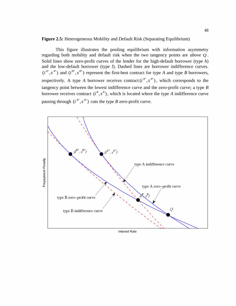
48

Figure 2.5: Heterogeneous Mobility and Default Risk (Separating Equilibrium)


regarding both mobility and default risk when the two tangency points are above Q .

Solid lines show zero-profit curves of the lender for the high-default borrower (type h)

and the low-default borrower (type l). Dashed lines are borrower indifference curves.

),( ** AA si and ),( ** BB si represent the first-best contract for type A and type B borrowers,

respectively. A type A borrower receives contract ),( ** AA si , which corresponds to the

tangency point between the lowest indifference curve and the zero-profit curve; a type B

borrower receives contract ),( BB si , which is located where the type A indifference curve

passing through ),( ** AA si cuts the type B zero-profit curve.

49

Figure 2.6: Heterogeneous Mobility and Default Risk (Separating Equilibrium)


regarding both mobility and default risk when the two tangency points are below Q .

Solid lines show zero-profit curves of the lender for the high-default borrower (type h)

and the low-default borrower (type l). Dashed lines are borrower indifference curves.

),( ** AA si and ),( ** BB si represent the first-best contract for type A and type B borrowers,

respectively. A type B borrower receives contract ),( ** BB si , which corresponds to the

tangency point between the lowest indifference curve and the zero-profit curve; a type A

borrower receives contract ),( AA si , which is located where the type B indifference curve

passing through ),( ** BB si cuts the type A zero-profit curve.

50

Table 2.1: Aggregated Effects of Mobility and Default

This table summarizes the aggregated effects of mobility and default risks. High

(low) mobility corresponds to flatter (steeper) indifference curves, and high (low) default

risk corresponds to steeper (flatter) indifference curves. From the lender’s perspective,

high (low) mobility corresponds to high (low) risk, and high (low) default corresponds to

high (low) risk. When borrowers are heterogeneous on both mobility and default risk, the

effects are combined. For instance, when a borrower is characterized by high mobility

and high default risk, we expect her indifference curves to be of medium slope. This

borrower is also very risky from the lender’s perspective.

DEFAULT

HIGH LOW

Steep/Risky Flat/Safe

MOBILITY

HIGH Medium Slope/Very Risky Very Flat/Medium Risk

Flat/Risky

LOW Very Steep/Medium Risk Medium Slope/Very Safe

Steep/Safe

51

Chapter 3

The Screening Roel of Mortgage Discount Points on

Transaction Costs19

The U.S. residential mortgage market is dominated by fixed-rate mortgages

(FRMs). One of the important benefits of the FRM is the borrowers’ prepayment option.

It allows a borrower to take advantage of lower rates through refinance. However, this

valuable feature requires monitoring by the borrower. To realize the benefit of the

prepayment option, a borrower must make correct refinancing decisions. In fact, properly

―maintaining‖ a FRM is far from a trivial task. Knowledge of interest rate trends and tax

rules is essential to gauge the potential benefit from refinancing. In addition,

sophisticated calculations are necessary to determine the right time to refinance.20

Moreover, refinancing itself is often costly and time-consuming. The substantial amount

of time and effort needed to search and bargain for refinancing opportunities is a

transaction cost, which is defined by Stanton and Wallace (1998) as ―a cost incurred by

the borrower but not received by the lender‖ (Stanton and Wallace 1998). The transaction

costs associated with refinance are different across borrowers for at least three reasons.

First, it may be less costly for a financially savvy borrower to exercise the prepayment

19 This chapter is derived from a co-authored paper with Brent Ambrose and Michael LaCour-Little entitled

―Do Mortgage Points Signal Mobility or Transactions Cost: Evidence from Securitization‖.

20 The complexity of optimal mortgage refinancing is reflected in the vast literature on option-based

mortgage pricing theory. Examples from this stream of literature include Kau, Keenan, Muller, and

Epperson (1992, 1993), Ambrose and Buttimer (2000).

52

option than for a naïve borrower. While some borrowers are equipped with superior

knowledge and quantitative skills to identify and take advantage of refinancing

opportunities, others may find it more costly to gather and mentally process the

information necessary to correctly refinance. Diversity of cognitive skills and financial

literacy has been extensively documented in economic literature. Older and less educated

individuals appear to have lower cognitive abilities and are more likely to make mistakes

on financial calculations.21

Limited financial literacy appears to be correlated with low

income, less education, older age and minority status.22

Second, borrowers may also

differ with respect to their search costs. High search costs may be attributable to the lack

of access to valuable information sources such as the internet, newspaper, and financially

savvy relatives and friends. Highlighting the importance of information sources and

search skills, Brown and Goolsbee (2002) find that lower life insurance premiums are

associated with greater internet usage. A similar pattern was also identified in the

residential housing markets. First-time and out-of-town buyers, who normally have

limited experience and information, appear to pay a substantial and persistent price

premium.23

Analogously, one could expect better information and search skills may

reduce the cost of refinancing. Finally, borrowers may differ in their opportunity costs.

Given the time-consuming nature of the refinancing process, individuals with greater

21 See Agarwal, Driscoll, Gabaix and Laibson (2007), Christelis, Tullio, and Padula (2006), Korniotis and

Kumar (2008a, 2008b).

22 See Hogarth and Hilgert (2002), Lusardi and Mitchell (2007), Lusardi and Tufano (2008), Bucks and

Pence (2008).

23 See Myer, He and Webb (1992), Turnbull and Sirmans (1993), Watkins (1998), and Lambson, McQueen

and Slade (2004).

53

opportunity costs would deem refinance more costly than others. I sketch a simple model

to show that when the transaction costs associated with refinance are heterogeneous

across borrowers and are unobservable, the mortgage market resembles the insurance

market delineated by Rothschild and Stiglitz (1976). I show that there exists a separating

equilibrium such that borrowers with higher (lower) transaction costs pay more (less)

discount points to obtain a lower (higher) interest rate.24

This equilibrium is also

characterized by the low-cost (high-prepayment-risk) borrower imposing a negative

externality on the high-cost (low-prepayment-risk) borrower.

The theory indicates that borrowers with high transaction cost, those who are

slower to refinance in the face of declining interest rates, tend to select more discount

points. In contrast, conventional mobility theory suggests that discount points are a signal

of the borrower’s expected mobility.25

Specifically, borrowers with smaller (greater)

expected probability of relocation select more (fewer) points. It is possible that the

borrower’s points-coupon choice is jointly determined by his transaction costs and

mobility. Given this potential dual screening role, it remains unclear that how lenders

interpret the signals generated from realized points-coupon choices. Thus, in contrast to

previous studies that focus solely on the borrower’s choice, I empirically study the

screening role of discount points from the lender’s perspective. I ask the question: Is the

empirically observed points-coupon tradeoff intended for screening mobility or

transaction costs? If discount points signal unobserved borrower characteristics,

24 Henceforth, high-cost borrowers and low-cost borrowers.

25 See Dunn and Spatt (1988), Chari and Jagannathan (1989), Yang (1992), Brueckner (1994), LeRoy

(1996) and Stanton and Wallace (1998).

54

transaction costs, or mobility, then I expect originators to use this information in making

securitization decisions. Thus, I investigate the relation between transaction costs and

securitization decisions to infer if mortgage originators sort loans based on transaction

costs.

As suggested by the model, paying points signals greater transaction costs. One

could then use discount points to measure transaction costs and examine whether they are

correlated with securitization decisions. However, discount points can also be correlated

with expected mobility, which lenders may also deem important. This mixed screening

function prevents a clear-cut interpretation on what discount points signal even if loans

are securitized based on how many points were paid at the origination. Thus, to achieve a

more informative test, I first separate the two effects by constructing an alternative

measure of transaction cost called excess yield spread, which is based on the

―overvaluedness‖ of a loan. A borrower is more likely to hold an overvalued loan if she is

subject to high transaction costs, that discourage her from searching and bargaining for

better mortgage contracts. Therefore, I expect this group of borrowers to also face

relatively high costs at the time of refinance. More importantly, the ―overvaluedness‖ of a

loan is unlikely correlated with low mobility. In fact, a longer expected holding period is

likely to induce more extensive search and bargaining. To establish the validity of the

measurement, I examine the connection between excess yield spread and prepayment

patterns. I find that borrowers holding overvalued mortgages are less likely to prepay,

and this reduced tendency is attributable to their sluggish response to declining market

interest rate. These results support the conjecture that excess yield spread serves as a

valid measurement of borrower transaction costs.

55

Equipped with a clearer measure of transaction costs, I can infer what discount

points signal from the mortgage originator’s perspective. I compare the effects of excess

yield spread and the amount of discount points on the likelihood of a loan being

securitized. I find that overvalued mortgages and ones with more discount points are both

more likely to be retained in originator’s portfolio (not securitized). This result indicates

that lenders are more likely to securitize loans originated by borrowers with higher cost

of refinance.

Related Literature

Mortgage-points choice has stimulated research interest from economists for

decades. For example, Dunn and McConnell (1981) first suggested that mortgage points

serve as a backdoor prepayment penalty for the lender to charge for the embedded

prepayment option. In contrast, Kau and Keenan (1987) pointed out that tax

considerations may play a crucial role in determining points paid on purchase loans.26

Because discount points may be deducted all at once at origination while the interest rate

deduction is spread across the life of the loan, borrowers with high marginal tax rates are

more willing to pay points in order to receive a low interest rate.

However, the majority of the mortgage-points literature focuses on borrower

mobility as the primary determinant. Pioneered by Dunn and Spatt (1988), an array of

studies followed this mobility tradition in explaining the widely observed points-coupon

menu. The basic intuition proposed by Dunn and Spatt (1988) is that borrowers who

26 Points paid for purchase loan are deducted at the year of origination, points paid for refinance loan are

amortized over the life of the loan.

56

expect to move soon benefit less from discount points. When offered a points-coupon

menu, high-mobility borrowers will self-select into mortgages with low points and high

coupons. This intuition was further modeled by Chari and Jagannathan (1989), Yang

(1992), and Brueckner (1994). To explain the observed points-coupon trade-off, Chari

and Jagannathan (1986) appeal to income uncertainty. In their model, relocation is

associated with favorable future income. Thus, paying discount points is viewed as

insuring against the low-income state. When the good state (relocation) occurs, the

benefit from points (low interest rate) is forfeited. Their model predicts that mobile

borrowers select loans with high points, a result contradicting other mobility-based

theories and empirically observed correlation between discount points and mobility

(Brueckner 1994, and Clapp, Goldberg, Harding, and LaCour-Little 2001). Allowing for

an arbitrarily large lender profit, Yang (1992) shows that it is possible to achieve a

separating equilibrium where borrowers with longer (shorter) expected residence in their

houses pay more (less) points. Brueckner (1994) constructs a two-period model to

consider the effect of information asymmetry on borrower mobility. In a competitive

market, when borrowers differ only in their probability of moving midway through the

term his mortgage, there exists a separating equilibrium such that high-mobility

borrowers choose low-points/high-coupon contracts from the available menu.

While mobility remains the theme, more recent studies by LeRoy (1996) and

Stanton and Wallace (1998) elevate the sophistication of the mortgage-points analysis by

incorporating the idea of financially motivated prepayment. LeRoy (1996) incorporates

both mobility- and interest-rate-motivated prepayments. The model achieves a semi-

pooling equilibrium, where the least mobile borrowers are separated from the rest of the

57

pool. Stanton and Wallace (1998) emphasize the transaction costs of refinancing, which

is defined as the costs incurred by borrowers but not received by the lender. They show

that with information asymmetry regarding borrower mobility, such costs are essential to

construct a separating equilibrium. Consequently, borrowers are fully separated based on

their mobility. Sedentary (mobile) borrowers select higher (lower) points and lower

(higher) interest rates.

A number of studies have supplied empirical support to the mobility-based

explanation. Brueckner (1994) constructs a mobility measure using a linear combination

of borrower characteristics (e.g. age, marital status, etc.) and shows that high mobility is

associated with taking loans with more discount points. As one of the few studies that

uses data that can distinguish between mobility related payoffs and refinancing, Clapp, et

al. (2001) find that paying discount points is associated with a reduced probability of

moving.

Nevertheless, transaction costs are often assumed to be homogeneous. (e.g.

Stanton and Wallace 1998). Although the influence of heterogeneous costs of refinancing

has not been theoretically acknowledged, some studies have explored its effect

empirically. Pavlov (2001) approximates transaction costs using refinancing history, loan

documentation, and discount points selection. He finds that higher transaction costs are

associated with lower refinancing probability. Using a data set containing both points and

loan termination information, Chang and Yavas (2008) find that borrowers who choose to

pay more points are less likely to refinance in the future, and when they do, they

refinance later than borrowers who choose to pay fewer points. On the other hand, they

58

find no correlation between paying discount points and the probability of moving. The

authors interpret their findings as evidence supporting heterogeneous transaction costs.

The use of loan ―overvaluedness‖ to measure transaction costs is inspired by the

literature on price premium in the real estate market. A number of studies have shown

that residential mortgages may not be uniformly priced. Carlin (2009) argues that despite

the large number of firms in the retail financial market, a firm can preserve market power

and charge a price above marginal cost by strategically increasing the complexity of their

price structure. As a result, naïve consumers pay a higher price than the informed ones.

Carlin (2009) shows that price dispersion can persist and even enlarge as the market

becomes more competitive. Woodward (2003, 2008) finds that households tend to pay

higher broker fees on mortgages with points, and that college education is associated with

a substantial reduction in average broker fees.

The existence of price premium has also been extensively documented in

residential property transactions. First-time and out-of-town buyers appear to pay a

substantial and persistent price premium, which may be attributable to buyer

characteristics such as experience, search costs, and bargaining power (Myer, et al. 1992,

Turnbull and Sirmans 1993, Watkins 1998, and Lambson, et al. 2004). Another stream of

literature complements these findings by showing that overpaid properties are associated

with a greater likelihood of mortgage delinquency (Calem and Wachter 1999), default

(LaCour-Little and Malpezzi 2003, Noordewier, Harrison and Ramagopal 2001), and

foreclosure (Ong, Neo, and Spieler 2006). Since households make both home purchase

and financing decisions, it is reasonable to believe the disadvantaged consumer group is

59

more likely to overpay, and such mortgages are associated with adverse outcomes (e.g.

slower refinance and higher default probability).

This study is also related to the literature on securitization. The incentive of

securitization may be attributable to information asymmetry (DeMarzo and Duffie 1999)

and regulatory arbitrage (Calem and LaCour-Little 2004). DeMarzo and Duffie (1999)

suggest that to overcome asymmetric information, it may be optimal for a better-

informed lender to retain loans with high degree of information asymmetry. Calem and

LaCour-Little (2004) argue that the required level of regulatory capital imposes a burden

on banks and creates incentive for securitizing mortgages with limited default risk.

Consistent with this view, Ambrose, LaCour-Little, and Sanders (2005) find that loans

retained in originator’s portfolio are more likely to default but less likely to prepay. I

compliment the securitization literature by showing how transaction features, such as

discount points, may provide useful signals to lenders making portfolio decisions.

The Model

In this section, I present a simple model to illustrate the role of discount points as

a screening device for the cost of refinancing. Consider a competitive lending market, in

which lenders offer a menu of fixed rate mortgage (FRM) contracts with a variety of

combinations of initial interest rate 0i , and discount points s. In the first period, the

borrower obtains a mortgage of size L to purchase a house of value LP . To make the

model tractable, I suppress property price variation by assuming constant property value

over time, and normalize the loan amount L to $1 so that the term ―interest rate‖ and

60

―interest payment‖ can be used interchangeably. More importantly, s can then be

interpreted as the percentage of loan amount, which is consistent with how mortgage

points are assessed. The mortgage matures in the second period when the borrower is

required to repay the principal plus interest. Second-period interest rate i is assumed to be

stochastic. The density function of i is denoted by )( f , and its support is given by ],[ ii .

I assume borrowers are identical in all aspects except for the direct monetary and non-

monetary costs of refinancing (e.g. appraisal fees, title search time and inconvenience

etc.), denoted by c. A borrower may prepay the mortgage if the realized value of i is

sufficiently less than his contract rate 0i . The critical value of i, below which refinancing

is optimal, depends on individual’s transaction costs. A borrower optimally prepays when

i satisfies

cii 0 (3.1)

The left-hand side of (3.1) equals the savings obtained via refinancing. Equation (3.1)

indicates that optimal refinancing occurs when the benefit exceeds the cost. Rearranging

terms leads to the following rule of refinancing:

ciii 0

~ (3.2)

where i~

represents the critical interest rate that triggers refinancing.

The optimality of this refinancing rule can be verified directly from borrower’s

objective function. Borrowers are risk-neutral and discount future cash flows by a factor

of 1 . Y denotes the exogenous component of wealth, which equals the borrower’s

initial endowment and discounted future income. Given risk-neutrality, the borrower’s

utility equals the expected discounted value of wealth

61

i

i

i

idiifiLPdiifciLPsLPY ~ 0

~

)()()()()( . (3.3)

In the first period, a borrower incurs down payment )( LP and discount points s. If the

second-period realized interest rate is between i~

and i , the borrower prepays to obtain

the favorable interest rate. However, refinancing comes with a cost c. If the second-

period realized interest rate is between i and i~

, the borrower repays the original loan

with principal and interest 0iL . To verify the refinancing rule (3.2) is optimal, (3.3) is

differentiated with respect to i~

. The first-order condition yields cii 0 , which implies

the optimal threshold for refinancing is cii 0

~. Substituting ci 0 for i

~ in (3.3), the

borrower’s utility can be written as

i

ci

ci

idiifiLPdiifciLPsLPYisu

0

0

)()()()()(),( 00 . (3.4)

The lender is also assumed to be risk-neutral and has a discount rate of 1 .

Hence, lender’s objective function is the expected discounted value of profit from the

mortgage loan.

i

ci

ci

idiifiLdiifiLsLis

0

0

)()()()(),( 00 (3.5)

In the first period, the lender transfers the loan amount minus the discount points to

borrower. If second-period interest rate falls below ci 0 the lender earns the current

market interest rate, which is less than the contract rate. Alternatively, if second-period

interest rate is above ci 0 , the lender earns the contract rate 0i .

To characterize the competitive market equilibrium, I first examine the

indifference curve of the borrower and the iso-profit curve of the lender. These curves

62

describe the borrower’s and lender’s trade-offs between discount points s and contract

rate 0i , respectively. To derive the slope of borrower’s indifference curve, I implicitly

differentiate 0i with respect to s holding ),( 0isu constant. Thus, it follows that

0

)(

1

0

0

0

i

ci

i

su

diifu

u

s

iMRS

. (3.6)

Hence, the indifference curves are downward sloping. This indicates that, from the

borrower’s perspective, the disutility resulting from paying points must be compensated

through a lower contract rate in order to remain on the same indifference curve. It is also

clear that uMRS is horizontal parallel indicating that the borrower’s indifference curves

have the same slope for a given 0i .27

In addition, the indifference curves are convex

because 00 iMRSu , that is, as 0i increases, the slope of indifference curves become

smaller (more negative). To focus on the influence of refinancing costs on a borrower’s

choice of discount points, (3.6) is differentiated with respect to c, and it follows that

0 cMRSu . In other words, as c increases, uMRS becomes larger (less negative).

Intuitively, a larger refinancing cost c induces a decline in the optimal threshold of

refinancing. With reduced probability of refinancing, the borrower is more willing to

trade discount points for a low contract rate. Thus, the indifference curves become flatter

as c increases.

To derive the slope of lender’s iso-profit curves, 0i is implicitly differentiated

with respect to s holding profit constant. The slope is given by

27 To see this, notice that (3.6) is independent of s.

63

)()(

1

00

0 cicfdiif

MRSi

ci

i

s

. (3.7)

Following Brueckner (2000) and Harrison, Noordewier, and Yavas (2004), I make the

simplifying assumption that the second-period interest rate is uniformly distributed. With

)( f being uniform, the slope of iso-profit curves become

)( 0ii

iiMRS

(3.8)

(3.8) is negative for ii 0 , but the iso-profit curve becomes positively sloped if ii 0 .

To focus on more realistic situations when MRS is downward sloping, I further impose

the restriction that 0i must be strictly less than i . The slope of borrower’s indifference

curves in the uniform case can be obtained via substituting for )( f in (3.6). It follows

that

)]([ 0 cii

iiMRSu

(3.9)

I first consider the situation when all borrowers share an identical level of

transaction costs. The assumption of a competitive market implies that the equilibrium

mortgage contract must lie on the zero-profit line, defined by 0),( 0 is . Borrower

utility is greater on lower indifference curves (fewer points and lower interest rate). Thus,

the point where the lowest indifference curve is tangent to the zero-profit curve gives the

equilibrium contract. The value of 0i at the tangency point can be solved via equating

(3.8) and (3.9). It follows that

64

cii*

0 (3.10)

With the restriction that ii 0 , must hold for this solution to be admissible. The

optimality requires that the zero-profit curve is more convex than the indifference curves.

This requirement is satisfied with )( f being uniform.28

I now study the situation when borrowers are different with respect to their costs

of refinancing. Suppose there exist two types of borrowers: borrowers with high

refinancing costs and borrowers with low refinancing costs. The costs of refinancing are

hc and hl cc respectively for high- and low-cost borrowers. Substituting hc and lc in

(3.5) yields two utility functions that are different in slope. Because 0 cMRSu , the

high-cost borrower’s indifference curve passing through a given ),( 0is point is flatter

than the low-cost borrower’s indifference curve. This fact is critical in deriving

equilibrium contracts. The flatter indifference curves of high-cost borrowers suggest that

they are more willing to trade discount points for a lower interest rate.

Heterogeneous refinancing costs also alter the relative position of the zero-profit

curves. The difference in the heights of the lender’s zero-profit curves can be obtained by

setting (3.5) to zero and differentiating, yielding 0

//0 icci . Since 0c , this

derivative is negative when the zero-profit curves are downward sloping )0(0i ,

implying that the high-cost borrower’s zero profit curve is always lower than the low-cost

28 The slope difference between iso-profit lines and indifference curves is negative (positive) when 0i is

less (greater) than *

0i . It indicates that the zero-profit curve is flatter than the indifference curve for *

00 ii

and steeper for *

00 ii .

65

borrower’s curve. The intuition is that the low-cost borrower is more likely to prepay,

thus a higher interest rate has to be charged to them for any given level of s to maintain

zero profit.

The first-best contracts are those that would be offered by a lender with perfect

information on borrower’s transaction costs. These contracts ensure that the lender makes

zero profit and each borrower’s utility is maximized. They are obtained by solving the

utility maximization problem of each borrower subject to their respective lender’s zero-

profit conditions. However, the first-best contracts are not always feasible for two reasons.

First, a lender usually does not possess perfect information on each borrower’s

refinancing cost. Second, even when individual characteristics (e.g. age, gender, and

education) are correlated with the borrower’s cost of refinancing and may be used to

obtain estimates of c, legal restrictions may prevent lenders from practicing price

discrimination based on such characteristics. In this case, all borrowers must be presented

with a menu of loans with the same points-coupon combinations.

To identify the mortgage market equilibrium under asymmetric information, I

follow the standard argument of Rothschild and Stiglitz (1976), who define an

equilibrium as a set of contracts satisfying two conditions. First, the lender earns zero

profit on all contracts. Second, no contract outside the given set attracts borrowers while

making a non-negative profit. I argue that there exist a separating equilibrium that

satisfies these conditions, and this equilibrium is characterized by borrowers with high

transaction costs paying more points to obtain a lower interest rate, and borrowers with

low transaction costs paying fewer points and receiving a higher interest rate.

66

To establish the argument, I first rule out the existence of a pooling equilibrium,

where both borrower types are offered the same contract. The zero-profit condition

implies that a pooling contract ),( 0

pp is must lie between the zero-profit curves in Figure 1.

In this case, the lender must make negative profit on low-cost borrowers and offset it

using positive profit made from high-cost borrowers. Such a contract does not represent

an equilibrium because there exist alternative contracts that attract high-cost borrowers

while making positive profit. Such contracts, located to the southeast of ),( 0

pp is , lie

above the low-cost indifference curve but below the high-cost curve passing through

),( 0

pp is . These contracts will attract only high-cost borrowers and earn a positive profit.

The existence of such contracts is ensured by the flatter slope of the high-cost

indifference curve.

The only remaining possibility is to have a separating equilibrium, where distinct

contracts are assigned to different borrower types. Market competitiveness implies that

the zero-profit conditions for both borrower types must be satisfied. In addition, the

equilibrium contracts must separate the two types of borrower by satisfying the revelation

principle. Collectively, these imply the following conditions.

,0),( lll si

(3.11)

,0),( hhh si

(3.12)

),,(),( hhllll siUsiU

(3.13)

),,(),( llhhhh siUsiU

(3.14)

67

(3.11) and (3.12) imply that the equilibrium contract for each type must lie on their

respective zero-profit curve. (3.13) and (3.14) state that the mortgage contract intended

for a given borrower type is chosen by that type. In other words, no borrower type has an

incentive to imitate the other in order to obtain greater utility. Since the low-cost, zero-

profit curve lies above the high-cost, zero-profit curve, it must be the case that (3.13) is

binding and (3.14) is not. Hence, the lender can offer low-cost borrowers their first-best

contract ),( *

0

* ll is without attracting high-cost borrowers. ),( *

0

* ll is corresponds to the

tangency points between the lowest indifference curve and the zero-profit curve. On the

other hand, the high-cost, first-best contract ),( *

0

* hh is if offered, will attract both types

and result in negative lending profit. Thus, the equilibrium contract received by the high-

cost borrower is located where the low-cost indifference curve passes through ),( *

0

* ll is

and cuts the high-cost zero-profit curve. This contract, which is denoted ),( *

0

* hh is , is

shown in figure 3.1. In this case, low cost borrowers are indifferent between ),( *

0

* ll is and

),( 0

hh is . The simultaneous offering of ),( *

0

* ll is and ),( 0

hh is satisfies the zero-profit

conditions and the incentive compatibility constraints.

It is clear that in equilibrium, high-cost borrowers select a contract with greater

mortgage points than low-cost borrowers. This differentiated mortgage choice arises from

the negative externality generated by information asymmetry. It is clear that low-cost

borrowers receive their first-best contract ),( *

0

* ll is , and their welfare is unaffected by

asymmetric information. In contrast, high-cost borrowers are deprived from obtaining

their first-best contract ),( *

0

* hh is and offered contract ),( 0

hh is , which is inferior to the

68

outcome under full information. This is consistent with the standard screening model that

high-risk types (low-cost borrowers) impose a negative externality on low-risk types

(high-cost borrowers).

Hypotheses Development

In this section, I develop hypotheses that are used in my empirical investigation.

The main challenge comes from the fact that my transaction-costs based theory is not the

only possible explanation for why borrowers pay discount points. In fact, previous

literature posits the heterogeneity of expected mobility as the reason for the observed

coupon-points trade-offs. Ambiguity arises from the fact that prepayment may come from

moving or refinancing. For instance, the model implies that borrowers with relatively

greater transaction costs rationally pay more discount points, and loans held by this group

of borrowers are characterized by delayed refinance. Thus, one could test whether or not

the amount of discount points paid at origination leads to a reduced probability of

prepayment. Unfortunately, such evidence is circumstantial at best, because discount

points may also signal mobility. Mobility theory suggests that low-mobility borrowers

should pay more discount points. Because prepayments resulted from refinance and

relocation are indistinguishable in the data, it is inconclusive which factor, mobility or

transaction costs, causes the reduced likelihood of prepayment. Furthermore, with this

mixed screening role of discount points, examining its effect on securitization decisions

will not be fruitful because I do not know whether such an impact is attributable to

transaction costs or mobility.

To distinguish the effects of mobility from transaction costs, I carry out a two-step

process. In the first step, I construct an alternative measure, excess yield spread, to gauge

69

borrower’s cost of refinancing. I provide empirical evidence that this measure indeed

captures borrower transaction costs. More importantly, this new measure is not subject to

the ambiguity caused by mobility and transaction costs working in the same direction.

Thus, in the second step, I determine whether or not lender securitization decisions are

impacted similarly by excess yield spread and discount points. Because excess yield

spread is a cleaner measure of transaction costs, juxtaposing it with discount points will

provide evidence for the motivation of offering the coupon-points menu.

I discuss the method of constructing excess yield spread in the next section.

However, the rationale behind such a measure is rather straightforward. Excess yield

spread gauges the relative ―overvaluedness‖ (or ―undervaluedness‖) of a loan. Greater

excess yield spread indicates that a borrower paid a relatively higher premium in terms of

interest rate for his mortgage. Because this higher premium is unexplained by standard

underwriting criteria (e.g. credit score, income, and LTV ratio) and discount points, it is

likely to reflect unobserved heterogeneity in transaction costs. I draw an analogy from the

well documented price premium phenomenon in the residential property market. First-

time and out-of-town buyers usually pays a substantial and persistent price premium,

which may be attributable to buyer characteristics such as experience, search costs, and

bargaining power.29

Because households make both home purchasing and financing

decisions, it is reasonable to expect borrowers with greater search costs and information

disadvantage also search less extensively for mortgages. As a result, these borrowers are

more likely to overpay for their loan. Similarly, borrowers with greater opportunity costs

29 See Myer, et al. (1992), Turnbull and Sirmans (1993), Watkins (1998), and Lambson, et al. (2004).

70

would also search and bargain less and pay a larger interest premium. Provided

transaction costs continue to influence future financial decisions, excess yield spread can

serve as a priori measure of the borrower’s cost of refinancing.

The model assumes that the interest-coupon trade-off at the wholesale level is

competitively priced. To maintain simplicity, I do not model the role of financial

intermediaries. In reality, the price premium may arise from the fact that mortgages are

originated through distinct channels (e.g. mortgage brokers verses retail lenders). While

mortgage funds are homogeneous and supplied in a competitive national market, the

service on obtaining it may be a local good and tends to be heterogeneous. I view the

price premium in the mortgage market primarily as a result of compensating financial

intermediaries for performing their market function. Thus, the existence of a price

premium does not contradict the assumption that the mortgage market is competitive at

the wholesale level. For instance, a mortgage broker who is connected to multiple lenders

may be able to search more efficiently on behalf of his customer. Such ―match-making‖

functions must be compensated and may take the form of a greater interest premium. On

the other hand, a mortgage broker may also have an incentive to steer borrowers to loans

that offer greater compensation.30

A loan officer paid on commission would be subject to

a similar agency problem. While the role of financial intermediaries is not the subject of

this study, I believe superior financial sophistication, better search skills, and greater

information reduce direct and indirect costs associated with financial intermediaries.

30 See Jackson and Barry (2001), LaCour-Little (2009), and Woodward (2008).

71

Obviously, the validity of using excess yield spread to measure transaction costs

requires empirical justification. If higher excess yield spread captures transaction costs, it

should be correlated with a lower likelihood of prepayment. More importantly, this

reduced tendency of prepayment should stem from increasingly slower refinance. This

rationale can be viewed from equation (3.2). Larger refinancing cost c lead to a decline of

the threshold interest rate i~

, which implies that high-cost borrowers will wait for a larger

rate reduction before they refinance. This translates to a reduced sensitivity of

prepayment to interest rate reduction. Hence, I construct the following hypothesis to test

the validity of excess yield spread as a measure of transaction costs:

H1: Loans with greater excess yield spread are less likely to prepay, and this reduced

tendency of prepayment is attributable to a lower sensitivity of prepayment to

interest rate reduction.

I are aware that the likelihood of holding overvalued loans may not be

independent from expected mobility. However the effects of mobility and transaction

costs on excess yield spread are likely to be in opposite directions. If borrowers differ in

their mobility but are relatively homogeneous in transaction costs, high-mobility

borrowers, who are more likely to prepay, would also be more likely to hold overvalued

loans. This is precisely the opposite of the hypothesis that loan ―overvaluedness‖ is

negatively related to the tendency to prepay. Having a shorter expected holding period,

high-mobility borrowers would gain less from costly search and bargaining. In other

words, expecting to relocate soon, high-mobility borrowers are less bothered by paying a

72

greater interest premium. Therefore, even if mobility also affects excess yield spread, it

strengthens the power or my test by making the hypothesized relation less evident.

The second step involves studying the connection between transaction costs and

securitization decisions. Securitization transforms heterogeneous and illiquid individual

loans into liquid and marketable securities. The securitization of residential mortgages

usually involves the originator retaining a portion of their originated loans and selling the

rest to the secondary market. Because mortgage originators are sophisticated financial

institutions and, more importantly, the designers and the user of the coupon-points menu,

they are able to interpret realized points-coupon combinations and identify otherwise

unobserved borrower characteristics (e.g. mobility or transaction costs). Therefore,

analyzing securitization decisions helps understand what information is conveyed by

discount points to mortgage originators. I expect the originator to sort loans based on

excess yield spread and the amount of discount points paid if 1) transaction costs are

important in determining whether or not a particular mortgage is securitized; and 2) the

points-coupon combinations serves effectively as a screening device of borrower

transaction costs.

I first examine whether overvalued loans are more or less likely to be retained. I

do not impose an expected sign on this correlation. As long as loans are sorted based on

excess yield spread, transaction costs must be important in making securitization

decisions. I then see if discount points have a similar effect. If transaction cost is an

important consideration for making securitization decisions, then discount points and

excess yield spread should have a consistent effect on securitization decisions, as they are

alternative measures of transaction costs. On the other hand, if the originator emphasizes

73

mobility and sorts mortgage points based on it, discount points and excess yield spread

should exhibit opposite effects on the securitization decision. This is because paying

greater discount points signals lower mobility but high ―overvaluedness‖ is likely

associated with high mobility. It is unlikely the originator makes securitization decisions

based on mobility yet treats loans with more points and greater excess yield spread in a

similar manner. Such a behavior lacks logical consistency. Thus, I formulate the

following hypothesis:

H2: Securitization decisions made on loans originated with more discount points and

loans with greater excess yield spread are consistent.

Empirical Analysis

Data

The data comes from Ambrose, et al. (2005), and consist of event histories of

25,520 conventional fixed rate mortgages originated between January 1995 and

December 1997 and followed through October 2000. The data includes loans for

refinancing as well as loans for home purchase. For each mortgage in the sample, I have

relatively complete micro-level loan information and borrower characteristics. Available

loan information include the time and state of origination, loan amount, coupon rate,

loan-to-value (LTV) ratio, and, most importantly, discount points paid at the time of

origination. The data set also contains information on borrower characteristics such as

credit score, age, and income. Finally, the data set also has information on whether the

loan was subsequently retained in the originator’s portfolio, sold to the GSEs, or sold as

74

private label MBS. Table 3.1 reports the summary statistics on the loan characteristics of

the sample. A rather noticeable pattern is that the average discount points are consistently

higher for loans that are not securitized. The difference is quite substantial in 1996 (0.979

for retained verses 0.556 for securitized) and in 1997 (0.799 for retained verses 0.422 for

securitized). Both are significant at 1% level. Securitized loans appear to consistently

have to have relatively low LTV and higher borrower credit scores as compared to

portfolio loans (significant at 1% for all years). Borrower income is also greater on

average for securitized loans (significant at 1% for year 2005 and 10% for year 2007).

Excess Yield Spread and Prepayment

The available coupon-points combinations emerge from the mortgage market

equilibrium. Todd (2001) uses a simultaneous equation model to capture the fact that

mortgage rate and discount points schedule are jointly determined. I apply a similar

methodology and estimate the following simultaneous equations in order to determine

whether or not a particular loan is undervalued or overvalued.

sDISCPTSPREAD 1Xa')ln( 10 (3.15)

dSPREADDISCPT 2Xb')ln(10 (3.16)

SPREAD is the mortgage yield spread. Following Merton (1974) I define the mortgage

yield spread as the difference between the yield and the risk-free rate. Accordingly, I

proxy the yield spread using the effective mortgage yield calculated over a 10-year

holding period less the 10-year treasury rate, and DISCPT is the discount points recorded

as a percentage of original outstanding balance. a is a row vector of coefficients, and X1

75

is a vector of determinants of mortgage yield. Similarly, b is a row vector of coefficients,

and X2 is a vector of variables that explains the borrower’s selection of mortgage points.

s and d are respectively the standard errors from equation (3.15) and (3.16). All

variables are measured at loan origination.

I follow Ambrose, LaCour-Little, and Sanders (2004) to specify equation (3.15).

Merton (1974) suggests that the yield spread is a function of the volatility of state

variables (interest rate and housing values) as well as the LTV ratio at origination.

Therefore, I include in a the interest rate volatility (MORTVOL) and housing price

volatility (HPIVOL). MORTVOL is defined as the standard deviation of the monthly 30-

year conventional mortgage rate over the previous 24 months.31

(HPIVOL) is defined as

the standard deviation of OFHEO state-level quarterly housing price index over the

previous two years. I also control for LTV ratio at origination (LTV), and the market

expectation of future interest rates as measured by the term structure (YLDCURVE),

which is defined as the 10-year Treasury bond rate minus the 1-year Treasury bond rate. I

also include in the set of explanatory variables an array of loan-specific characteristics at

origination including borrower’s credit score (FICO), borrower’s income (INCOME), and

conforming loan status (CONFORM).32

Following Ambrose and Pennington-Cross (2000)

and Ambrose, et al. (2004), I control for differences in state law regarding mortgage

default and foreclosure by including a set of dummy variables that classify states based

31 I obtain the 30-year conventional mortgage rate from the Federal Reserve Bank of St. Louis.

32 Following Ambrose, et al. (2005), I classify a mortgage as conforming if it was sold to the agencies, or if

the borrower’s FICO score is above 660 and the loan amount was below the conforming loan limit in place

at time of origination and the LTV is either less than 80 percent or the loan has private mortgage insurance

if the LTV is greater than 80 percent.

76

on judicial versus non-judicial foreclosure laws and deficiency versus non-deficiency

judgment states. q1 indicates states that have nonjudicial foreclosure available and allow

lenders to obtain deficiency judgments; q2 indicates states that have nonjudicial

foreclosure available but do not allow deficiency judgments; q3 indicates states that

require judicial foreclosure and allow deficiency judgments; and finally q4 indicates

states that require judicial foreclosure and do not allow deficiency judgments. Finally, I

also control for time and geographic related variations. To capture seasonal market

changes of mortgage origination, I include year and month indicator variables, which

respectively denote the year and month of origination. I also control for regional fixed

effect by a set of indicator variables constructed based on HUD 10-region classification.33

I include in X2 variables that are influential on borrower’s selection of mortgage

points. First, borrowers make contract choices based on market conditions. Therefore, it

is reasonable to control for macroeconomic variables such as interest rate volatility

(MORTVOL), housing price volatility (HPIVOL) and yield curve (Y LDCURV E). Second,

the decision of paying discount depends on a borrower’s cash availability. Thus, I use

borrower’s income (INCOME) and the loan-to-value (LTV) ratio to control for the

availability of financial resource at the time of origination. Third, because conforming

loans are subject to a lower cost of borrowing, one would expect conforming loans are

less likely to be prepaid. Thus, I control for the conforming loan status (CONFORM).

Finally, Brueckner (1994) shows that the borrower’s age and income, property value, and

geographical location are significantly correlated with mobility. Hence, I control for

33 The ten regions are New England, New York/New Jersey, Mid-Atlantic, Southeast, Midwest, Southwest,

Great Plains, Rocky Mountain, Pacific/Hawaii, and Northwest/Alaska.

77

borrower’s age (BWRAGE) and regional dummy variables. I also include the square of

BWRAGE to control for potential non-linear effects. Similar to the SPREAD equation, we

control for time fixed effects. I identify equation (15) using borrower’s age (BWRAGE)

and its square term (BWRAGE2), because lenders are prohibited by the Fair Housing Act

of 1968 to impose different conditions on mortgages based on age.34

We identify (16)

using borrower’s credit score FICO, because borrowers with difference credit scores are

provided with the same coupon-points menu.35

Notice that the borrower’s desired amount of discount points may not always be

positive.36

In the data, I observe non-zero value of DISCPT only if the borrower demand

positive points, and demand for negative points are censored. To overcome this problem,

I estimate equation (3.15) and (3.16) via two-stage procedure. In step one, the reduced

form of equation (3.15) is estimated by ordinary least squares, and the reduced form of

equation (3.16) is estimated with a tobit specification. In step two, the structural

estimation of equation (3.15) and (3.16) is performed using the predicted values of

SPREAD and DISCPT from the first step.

Table 3.2 reports the estimated results. The negative and statistically significant

coefficients of DISCPT in equation (3.15) and ln(SPREAD) in equation (3.16) confirm

34 The validity of our instruments is strengthened by the results from the overidentification tests. For both

versions of Sargan’s (1958) and Basmann’s (1960) tests of overidentifying restrictions, we fail to reject the

null hypothesis that BWRAGE and BWRAGE2 are valid instruments.

35 We conduct the test proposed by Stock and Yogo (2001) to guard against weak instrument problem. Our

instrumental variables appear to be strongly correlated with the endogenous variables. The F-statistics of

the correlations between the endogenous independent variable and the instrumental variables are 24.24 and

360.43 respectively for equation (15) and equation (16), which suggest that the weak instrument problem is

unlikely to be a concern.

36 Lenders may help pay for the entire or a part of closing cost using yield spread premiums (YSP). This

can be viewed as one way for borrowers to take negative discount points.

78

the inverse correlation between interest rate and discount points. This result is consistent

with Brueckner (1994), who also finds evidence for the points-coupon tradeoff. I denote

the prediction error of (3.15) as excess yield spread (EXSPD), and propose it as a

measure of borrower search cost. A larger (smaller) value of EXSPD indicates the loan is

relatively overvalued (undervalued) and the borrower is likely to have high (low)

transaction costs.

To check the validity of EXSPD as a measure of transaction costs, I empirically

examine the correlation between excess yield spread and prepayment. As stated in

hypothesis 1, EXSPD can be a valid measure of transaction costs, only if it exhibits a

negative correlation with the likelihood of prepayment. I estimate a competing risk

hazard model following the methodology used in Ambrose and Sanders (2003). A

borrower has the option to prepay, default, or remain current for any given period. I treat

mortgages that are still current at the end of the observation period as censored. Thus, I

define )3,2,1( jT j as the latent duration for each mortgage to be terminated during the

observation period by prepaying, defaulting, or remaining current (censored). Thus, the

observed duration, , is the minimum of the jT .

Conditional on a set of explanatory variables, jx , which may include static loan

characteristics at the time of loan origination as well as time-varying economic conditions,

and parameters, j , the probability density function (pdf) and cumulative density

function (cdf) for jT are

));|(exp();|();|( jjjjjjjjjjjj xrIxThxTf (3.17)

79

);|(exp(1);|( jjjjjjjj xrIxTF (3.18)

where r is an integer variable taking values in the set {1, 2, 3} representing the three

possible outcomes, jI is the integrated hazard for outcome j:

jT

jjjjjjj xshxTI0

);|();|( (3.19)

where jh is the hazard function.

The joint distribution of the duration and outcome is

));|(exp();|();|( 0 jjjjjjjjjjj xIxhxf (3.20)

where ),,( 321 xxxx and ),,( 321 and

3

1

0

j

jII is the aggregated

integrated hazard. Thus, the conditional probability of an outcome is

3

1

);|(

);|();,|Pr(

j

jj

jj

xh

xhxj

(3.21)

I assume a separate exponential hazard function for each mortgage outcome and estimate

(3.21) under a multinomial logit framework.

I include in the competing risk hazard model other factors that may impact

mortgage default and prepayment. In the contingent claim framework, the FRM contract

contains a prepayment option and a default option. A borrower minimizes the market

value of his outstanding loan via strategically exercising these two options. To capture

how much the prepayment option is ―in-the-money‖, I include in jx a variable, tRATE ,

which is defined as

m

t

m

t

c

tt

r

rrRATE

(22)

80

Where c

tr is contract rate at time t, and m

tr is the 30-year conventional mortgage rate at

time t. A relative increase in tRATE increases the likelihood of prepayment.

Theoretical mortgage literature indicates that the intrinsic values of the default

and prepayment options are jointly determined. The relative position of the default option

affects borrower refinancing strategy. Specifically, declines in property values increase

the probability of default and reduce the probability of prepayment. To account for the

competing nature of default and prepayment risk, I control for contemporary loan-to-

value (LTV) ratio, CLTV, which is computed as the ratio of the market value of the loan

to the market value of the property.

As suggested by Kau, et al. (1992, 1993), interest rate volatility also plays a

critical role in determining the value of the prepayment option. Hence, I account for

interest rate volatility by including the variable MORTVOL.I also control for housing

price volatility by include the variable HPIVOL. Following Ambrose and Sanders (2003),

I control for market expectation on future interest rate by including the slope of yield

curve (YLDCURVE).

I also control for array of loan and borrower characteristics at loan origination,

such as discount points (DISCPT), the loan-to-value ratio (LTV), borrower’s age

(BRWAGE), income (INCOME) and credit score (FICO) at origination. I include the set

of legal variables (q1-q4), constructed based on judicial versus non-judicial foreclosure

laws and deficiency versus non-deficiency judgment states, to control for differences in

legal environment. Finally, I control for time and regional fixed effects.

81

Table 3.3 presents the results of the competing risk hazard model. Consistent with

the first hypothesis, I observe a negative correlation between EXSPD and the probability

of prepay (significant at 1% level). This result shows that the effect of transaction costs in

determining EXSPD is likely dominating that of mobility, which tends to weaken the

observed association. The other interesting finding is that EXSPD increases the likelihood

of default (significant at 1% level). This result echoes previous studies that find that

borrowers with overpriced properties are more likely to become delinquent, default, or

experience foreclosure.37

It is consistent with the intuition that borrowers with less

experience, information, and bargaining power tend to pay a price premium in both

property and financial markets.

I further test my measurement by investigating the sensitivity of prepayment to

market interest rate fluctuations. The model predicts that borrowers with higher

transaction cost require greater rate reductions to cover their high cost of refinancing

before interest-rate motivated prepayment takes place. Hence, the prepayment behavior

of loans with greater EXSPD should be less sensitive to declining interest rate.

Operationally, I modify the competing risk hazard model by including an interaction term

of EXSPD and ΔRATE to capture the sensitivity of prepayment to interest rate. ΔRATE

indicates how much the prepayment option is ―in-the-money‖, which is positively related

to likelihood of refinance increases. This property is theoretically shown by option-based

mortgage models and also extensively documented by empirical studies on mortgage

termination. I are, however, interested in how this dependence varies across mortgages

37 See Calem and Wachter (1999), LaCour-Little and Malpezzi (2003), Noordewier, Harrison and

Ramagopal (2001), and Ong, Neo, and Spieler (2006).

82

with distinct ―overvaluedness‖. Specifically, I expect that mortgages with greater EXSPD

should have a smaller marginal change in the likelihood of refinance. Because borrowers

who overpaid for their loans have higher refinancing costs, they should wait for a

relatively larger interest rate reduction before they refinance. To capture this sensitivity, I

modify the original competing risk hazard model by creating an interaction term between

EXSPD and ΔRATE. The estimated coefficient of RATEEXSPD pinpoints this

differential marginal effect, and the model is supported if this coefficient is negative. To

examine other potential effects of transaction costs on the default and prepayment options,

I also include in the model interaction terms between EXSPD and the default option

)( CLTVEXSPD , interest rate volatility )( MORTVOLEXSPD , and housing price

volatility )( HPIVOLEXSPD .

Column 3 and 4 of Table 3.3 presents the results of the competing risk hazard

model investigating the sensitivity of refinance to interest rate. Consistent with the

hypothesis, the coefficient of RATEEXSPD is significantly negative (significant at 1

percent level). It shows that high-cost borrowers (the ones with overvalued mortgages)

are in fact less responsive to market interest rate reduction. This result is consistent with

Chang and Yavas (2009), who argue that the points-coupon trade-off is a viable screening

device for asymmetric transaction costs. They show that high-cost borrowers are less

likely to refinance, and when they do, they wait for a relative larger interest reduction as

opposed to others who did not pay points.

Consistent with empirical mortgage literature, I find support for the ―jointness‖ of

prepayment and default option. A larger interest rate reduction )( tRATE increases the

83

probability of prepayment but reduces the probability of default (both significant at 1%

level). Contemporary LTV (CLTV) reduces the likelihood of prepay (significant at 1%

level) but fails to exhibit a significant effect on default. I also find that loan and borrower

characteristics play an important role in determining default and prepayment risk.

Consistent with previous literature, I find that discount points (DISCPT) lead to reduced

probability of prepayment (significant at 1% level). Mortgages with high LTV ratios are

more likely to default and less likely to prepay (both significant at 1% level). Not

surprisingly, borrowers with better credit scores are more likely to prepay and less likely

to default (both significant at 1% level). Older borrowers are less likely to prepay

(significant at 1% level). High-income borrowers are more likely to prepay (significant at

1% level) and less likely to default (significant at 10% level). Finally, conforming loans

are associated with reduced probabilities of both default and prepayment (both significant

at 1% level).

Mortgage Points, Excess Yield Spread and Securitization Decisions

I now turn to testing the second hypothesis. To determine the probability that a

mortgage will be retained by the originator, I estimate the following logit model:

ZC ')1Pr( 110 DISCPTDISCPTPortfolio (3.23)

where DISCPT and EXSPD are the two measures of borrower transaction costs, and Z is

a set of control variables. If mortgages are sorted by the originator based on transaction

costs, one would expect 1 and 2 to have the same sign. A positive (negative)

correlation indicates that the originator tends to retain loans held by borrowers with high

84

(low) transaction costs. On the other hand, it may also be the case that 1 and 2 are

insignificant or having opposite signs. In this case, I would fail to find support to the

hypothesis that securitizations are made based on transaction costs.

Following Ambrose, et al. (2005), I also control for other factors that may have

impact on securitization decisions. I include in equation (3.23) macroeconomic variables

such as slope of the yield curve (YLDCURVE), interest rate volatility (MORTVOL), and

housing price volatility (HPIVOL). I also control for loan and borrower characteristics

including LTV ratio (LTV ), borrower’s credit quality (FICO), age (BWRAGE), income

(INCOME) and conforming loan status (CONFORM). I control for legal environment

using a set of legal variables (q1-q4), constructed based on judicial versus non-judicial

foreclosure laws and deficiency versus non-deficiency judgment states. Finally, I also

include regional and year dummy variables to control for time and regional fixed effects

(not reported).

Dionne, Gouriéroux, and Vanasse (2001) suggest that empirical evidence of

adverse selection takes the form of ―conditional dependence.‖ It would be preferable to

control for expected contractual choices in order to address potential problems of

misspecification. Thus, I include the predicted discount points PTCDIS ˆ estimated from

(3.15) and (3.16) as a control variable when estimating (3.23).

I find strong evidence that securitization decisions are made based on borrower’s

transaction costs. Both of the transaction costs measures EXSPD and DISCPT are highly

significant when included separately (column 1 and 2) and jointly (column 3) to explain

securitization decisions (all significant at 1% level). The positive association between

85

being retained in the originator’s portfolio and the transaction costs measures suggests

that the originator prefers loans held by high-cost borrowers. This result is also consistent

with Ambrose et al. (2005) who find that loans being retained are less likely to prepay. In

addition, I find that loans with high LTV and low borrower income are more likely to be

retained (both at 1% level). Not surprisingly, conforming loans are more likely to be

securitized.

Summary of Findings

I develop a theoretical model to show that transaction costs play an important role in

shaping mortgage market equilibrium. Specifically, when borrowers are different in their

cost of refinancing, there exists a separating equilibrium such that high-cost borrowers

pay more points to obtain a lower interest rate, and low-cost borrowers pay fewer points.

I further examine the empirical importance of heterogeneous refinancing cost. I find that

overvalued mortgages are less likely to be prepaid, and the prepayment pattern appears to

be less responsive to market interest rate reductions. This result suggests that borrower

costs of refinancing plays more critical role than expected mobility in determining the

likelihood of overpaying for a mortgage. Hence, loan overvaluedness can be valid

measure of refinancing costs. Furthermore, I find that mortgages with more points and

overvalued loans are both more likely to be retained in the originator’s portfolio. This

result indicates that the consideration of refinancing costs appear to have a greater impact

than mobility in determining the originator’s securitization decisions.

86

Figure 3.1: Mortgage-Points Choice with Asymmetric Information


asymmetry regarding refinancing cost. Solid lines show zero-profit curves of the lender

for high-cost borrower (type h) and low-cost borrower (type l). Dashed lines are borrower

indifference curves. Low-cost borrower receives contract ),( *

0

* ll is , which corresponds to

the tangency points between the lowest indifference curve and the zero-profit curve;

high-cost borrower receives contract ),( 0

hh is which is located where the low-cost

indifference curve passing through ),( *

0

* ll is cuts the high-cost zero-profit curve.

87

Table 3.1: Descriptive Statistics

This table presents the descriptive statistics of our sample. DISCPT is discount points paid at

origination. LTV is the loan-to-value ratio. FICO is borrower’s credit score. BRWAGE is borrower’s age.

INCOME is borrower’s income. We compare portfolio loans and securitized loans. Panel 1, 2, and 3

respectively show the comparison for loans originated in year 1995, 1996, and 1997. t-statistics and the

corresponding p-value on mean differences between portfolio loans and securitized loans are shown in

column 6 and 7.

Year of Origination: 1995

Portfolio Securitized

Mean Std. Dev Mean Std. Dev t-stat. p-value

DISCP T 0.643 0.799 0.604 0.852 -0.841 0.400

LT V 88.933 13.029 77.62 17.146 -

12.202 0.000 F ICO 694.362 62.774 717.405 58.598 7.156 0.000 BRW AGE 35.763 9.682 40.584 11.348 7.823 0.000 INCOME 52.574 55.267 63.609 59.034 3.428 0.000

% of Prepay 60.71% 43.73% % of Default 12.09% 4.20%

% of Still Current 27.20% 52.07% # of Observation 364 5875




DISCP T 0.979 0.842 0.556 0.8 -6.747 0.000 LT V 82.526 16.355 74.244 15.784 -5.97 0.000 F ICO 708.167 60.9 722.572 55.183 3.326 0.000 BRW AGE 40.421 11.448 41.757 11.315 1.491 0.136 INCOME 73.222 177.083 80.444 84.703 1.042 0.298






DISCP T 0.799 0.846 0.422 0.733 -7.44 0.000 LTV 79.177 16.808 74.244 15.784 -4.521 0.000 F ICO 696.906 67.227 722.724 55.305 6.735 0.000 BRW AGE 42.829 12.934 41.998 11.208 -1.062 0.288 INCOME 75.762 74.694 89.385 118.291 1.675 0.094



88

Table 3.2: Estimation of Excess Yield Spread

This table reports the two-stage regression estimates of the following system of equations.

sDISCPTSPREAD 1Xa')ln( 10

dSPREADDISCPT 2Xb')ln(10

SPREAD is the effective mortgage yield calculated over a 10-year holding period less the 10-year treasury.

DISCPT is discount points paid at origination. MORTVOL is the standard deviation of the monthly 30-year

conventional mortgage rate over the previous 24 months. HPIVOL is the standard deviation of OFHEO

state-level housing price index over the previous 24 months. LTV is the loan-to-value ratio. YLDCURVE

measures market expectation of future interest rate, which is defined as the 10-year Treasury bond rate

minus the 1-year Treasury bond rate. FICO is borrower’s credit score. INCOME is borrower’s income.

CONFORM is a dummy variable indicating conforming loan status (1 = Yes, 0 = No). BRWAGE is

borrower’s age. PROPVAL is the value of property at origination. q1-q4 are dummy variables constructed

based on judicial versus non-judicial foreclosure laws and deficiency versus non-deficiency judgment states.

Variable Estimate Std. Err. t-stat P > t

SPREAD Equation

DISCPT -0.620 0.087 -7.100 0.000

MORTVOL 0.177 0.155 1.150 0.252

HPIVOL 0.008 0.002 3.350 0.001

LTV -0.001 0.000 -4.340 0.000

YLDCURVE -0.115 0.042 -2.720 0.006

FICO 0.000 0.000 0.640 0.519

INCOME 0.000 0.000 -4.940 0.000

CONFORM -0.107 0.011 -9.650 0.000

q2 0.028 0.014 2.000 0.046

q3 0.104 0.020 5.090 0.000

q4 0.239 0.043 5.620 0.000

Intercept 0.690 0.103 6.720 0.000

DISCPT Equation

ln(SPREAD) -1.302 0.338 -3.850 0.000

MORTVOL 1.357 0.337 4.030 0.000

HPIVOL 0.015 0.005 3.040 0.002

LTV -0.005 0.001 -8.970 0.000

YLDCURVE -0.211 0.118 -1.790 0.074

INCOME -0.001 0.000 -9.450 0.000

CONFORM -0.205 0.026 -7.840 0.000

BRWAGE 0.016 0.004 3.880 0.000

BRW AGE2 0.000 0.000 -3.360 0.001

q2 0.135 0.030 4.440 0.000

q3 0.283 0.025 11.130 0.000

q4 0.638 0.066 9.710 0.000

Intercept -0.132 0.333 -0.390 0.693

89

Table 3.3: Competing-Risks Hazard Model of Mortgage Termination Outcomes

The competing risks model is estimated as a multinomial logit model assuming a quadratic

baseline hazard function. EXSPD is excess yield spread estimated from (3.15) and (3.16). ΔRATE is

defined as the mortgage rate reduction as a percentage of current market rate. CLTV is the ratio of the

market value of the loan to the market value of the property. MORTVOL is the standard deviation of the

monthly 30-year conventional mortgage rate over the previous 24 months. HPIVOL is the standard

deviation of OFHEO state-level housing price index over the previous 24 months. DISCPT is discount

points paid at origination. YLDCURVE measures market expectation of future interest rate, which is

defined as the 10-year Treasury bond rate minus the 1-year Treasury bond rate. LTV is the loan-to-value

ratio. FICO is borrower’s credit score. BRWAGE is borrower’s age. INCOME is borrower’s income.

CONFORM is a dummy variable indicating conforming loan status (1 = Yes, 0 = No). q1-q4 are dummy

variables constructed based on judicial versus non-judicial foreclosure laws and deficiency versus non-

deficiency judgment states. MONTH is the number of month since origination. Standard errors are shown in

parentheses below each regression coefficient. One, two, and three asterisks respectively denote

significance at 10%, 5%, and 1% level.

(1) (2)

Variable Prepay Default Prepay Default

EXSPD -0.198 1.136 1.518 0.152

(0.070)*** (0.207)*** (0.348)*** (0.820)

ΔRAT E 5.662 -1.264 5.817 -1.337

(0.130)*** (0.365)*** (0.133)*** (0.369)***

CLTV -0.604 0.428 -0.439 0.009

(0.224)*** (0.596) (0.245)* (0.871)

MORTVOL -3.325 -4.925 -3.213 -4.967

(0.156)*** (0.524)*** (0.158)*** (0.524)***

HPIVOL 0.044 0.097 0.046 0.096

(0.005)*** (0.015)*** (0.005)*** (0.015)***

EXSPD × ΔRAT E

-2.676 1.968

(0.596) (1.575)

EXSPD × CL V

-1.683 3.492

(1.309)*** (3.771)

EXSPD × MORTVOL

-3.073 1.477

(0.798)* (1.904)

EXSPD × HP IVOL

-0.044 0.059

(0.023)*** (0.058)

DISCPT -0.158 -0.081 -0.149 -0.086

(0.016)*** (0.042)* (0.016)*** (0.042)**

YLDCURVE -0.979 -1.272 -0.966 -1.281***

(0.045)*** (0.155)*** (0.045)*** (0.155)

90

Table 3.3: Competing-Risks Hazard Model of Mortgage Termination Outcomes (Cont.)

The competing risks model is estimated as a multinomial logit model assuming a quadratic

baseline hazard function. EXSPD is excess yield spread estimated from (3.15) and (3.16). ΔRATE is

defined as the mortgage rate reduction as a percentage of current market rate. CLTV is the ratio of the

market value of the loan to the market value of the property. MORTVOL is the standard deviation of the

monthly 30-year conventional mortgage rate over the previous 24 months. HPIVOL is the standard

deviation of OFHEO state-level housing price index over the previous 24 months. DISCPT is discount

points paid at origination. YLDCURVE measures market expectation of future interest rate, which is

defined as the 10-year Treasury bond rate minus the 1-year Treasury bond rate. LTV is the loan-to-value

ratio. FICO is borrower’s credit score. BRWAGE is borrower’s age. INCOME is borrower’s income.

CONFORM is a dummy variable indicating conforming loan status (1 = Yes, 0 = No). q1-q4 are dummy

variables constructed based on judicial versus non-judicial foreclosure laws and deficiency versus non-

deficiency judgment states. MONTH is the number of month since origination. Standard errors are shown in

parentheses below each regression coefficient. One, two, and three asterisks respectively denote

significance at 10%, 5%, and 1% level.

(1) (2)

Variable Prepay Default Prepay Default

LTV -0.006 0.007 -0.006 0.007

(0.001)*** (0.002)*** (0.001)*** (0.002)***

FICO 0.002 -0.010 0.002 -0.010

(0.000)*** (0.000)*** (0.000)*** (0.000)***

BRWAGE -0.014 0.000 -0.014 0.000

(0.001)*** (0.003) (0.001)*** (0.003)

INCOME 0.000 -0.002 0.000 -0.002

(0.000)*** (0.001)*** (0.000)*** (0.001)***

CONFORM -0.231 -0.318 -0.229 -0.318

(0.024)*** (0.075)*** (0.024)*** (0.075)***

q2 0.287 -0.041 0.285 -0.041

(0.042)*** (0.147) (0.042)*** (0.147)

q3 -0.187 0.075 -0.184 0.073

(0.036)*** (0.113) (0.036)*** (0.113)

q4 -0.366 0.540 -0.368 0.539

(0.097)*** (0.268)** (0.097)*** (0.269)**

MONTH 0.066 0.109 0.066 0.110

(0.003)*** (0.009)*** (0.003)*** (0.009)***

MONTH2 -0.001 -0.001 -0.001 -0.001

(0.000)*** (0.000)*** (0.000)*** (0.000)***

Intercept -4.594 0.455 -4.641 0.464

(0.193)*** (0.571) (0.194)*** (0.572)

91

Table 3.4: Mortgage Points, Excess Yield Spread, and Securitization Decisions

This table presents the estimates of the logit regression examining the relation between securitization decision

and discount points structures. The dependent variable is whether or not a mortgage was retained in the originator’s

portfolio (1 = Yes, 0 = No). EXSPD is excess yield spread estimated from (3.15) and (3.16). DISCPT is discount points

paid at origination. MORTVOL is the standard deviation of the monthly 30-year conventional mortgage rate over the

previous 24 months. HPIVOL is the standard deviation of OFHEO state-level housing price index over the previous 24

months. LTV is the loan-to-value ratio. FICO is borrower’s credit score. YLDCURVE measures market expectation of

future interest rate, which is defined as the 10-year Treasury bond rate minus the 1-year Treasury bond rate. BRWAGE

is borrower’s age. INCOME is borrower’s income. CONFORM is a dummy variable indicating conforming loan status

(1 = Yes, 0 = No). q1-q4 are dummy variables constructed based on judicial versus non-judicial foreclosure laws and

deficiency versus non-deficiency judgment states. Standard errors are shown in parentheses below each regression

coefficient. One, two, and three asterisks respectively denote significance at 10%, 5%, and 1% level.

Variable (1) (2) (3)

EXSPD 2.002 2.435

(0.242)*** (0.251)***

DISCPT 0.280 0.383

(0.044)*** (0.045)***

MORTVOL -0.187 0.902 -0.155

(1.595) (1.621) (1.637)

HPIVOL 0.040 0.042 0.038

(0.029) (0.030) (0.030)

LTV 0.018 0.020 0.019

(0.004)*** (0.004)*** (0.004)***

FICO -0.002 -0.002 -0.002

(0.001)** (0.001)* (0.001)**

YLDCURVE 1.051 0.987 1.078

(0.341)*** (0.339)*** (0.347)***

BRWAGE 0.007 0.007 0.007

(0.005) (0.005) (0.005)

INCOME -0.009 -0.008 -0.008

(0.001)*** (0.001)*** (0.001)***

CONFORM -2.357 -2.292 -2.304

(0.135)*** (0.137)*** (0.140)***

DÎCSPT -0.830 -0.902 -0.878

(1.060) (1.080) (1.108)

q2 -0.858 -0.825 -0.849

(0.236)*** (0.234)*** (0.244)***

q3 -0.577 -0.539 -0.600

(0.284)** (0.288)* (0.295)**

q4 0.606 0.448 0.472

(0.562) (0.567) (0.583)

Intercept -2.841 -3.644 -2.959

(0.787)*** (0.807)*** (0.806)***

N 25,808 25,520 25,520

Pseudo R2 0.221 0.214 0.225

92

Chapter 4

Bad Borrowers or Bad Loans? The Effect of Information

Asymmetry on the Choice of Prepayment Penalty

A mortgage contract often involves restrictions on prepayment. One such

restriction is the prepayment penalty. A prepayment penalty is a charge that a lender

makes when a borrower prepays the entire or a significant part of loan balance.

Conventional wisdom considers charging prepayment penalties as a way to reduce the

likelihood that lenders will have to reinvest the prepaid mortgage balance at a lower rate

(Ling and Archer, 2008). While commercial mortgage contracts in the United States

usually stipulate some form of restriction on prepayment, prepayment penalties on

residential mortgages have been a much more controversial topic. Extensive debate has

focused on the economic fairness of prepayment penalties. In other words, do borrowers

who accept prepayment penalties receive commensurate benefit? A prepayment penalty

reduces the value of a borrower’s prepayment option. As a trade-off, a mortgage with a

prepayment penalty usually has a lower interest rate than a contract without one.38

A

number of previous studies suggest that the offsetting economic benefit (e.g., lower

interest rate) is generally not sufficient to compensate the loss from the inability to

refinance.39

Other studies document that loans that have a prepayment penalty are

associated with more delinquencies, defaults, and property foreclosures.40

As a result,

38 See DeMong and Burroughs (2005) and LaCour-Little and Holmes (2008).

39 See Goldstein and Son (2003) and LaCour-Little and Holmes (2008).

40 See Danis and Pennington-Cross (2007) and Quercia, Stegman, and Davis (2007).

93

prepayment penalties have been viewed by many housing and consumer activists as being

―predatory‖ in nature. In light of the current housing crisis, prepayment penalties appear

to be extremely disturbing because predatory loans, such as the ones with prepayment

penalties, not only erode household wealth but also exacerbate foreclosure risk (Quercia

et al. 2007). In this study, I refer to the view that prepayment penalties increase default

risk as the predation hypothesis.

However, some economists argue that prepayment penalties may be welfare-

enhancing. For example, Chomsisengphet and Pennington-Cross (2006) point out that

prepayment penalties extend the duration of loans, reduce the loan-to-value (LTV) ratios,

and mitigate default risk. Mayers, Piskorski and Tchistyi (2009) show that prepayment

penalties improve welfare by ensuring longer-term lending contracts. In an environment

where borrowers’ creditworthiness stochastically evolves over time, longer-term

contracts help lenders insure against the risk that mortgage pools become

disproportionately composed of risky borrowers. The authors show that prepayment

penalties are particularly beneficial to risky borrowers by reducing default risk and the

cost of borrowing. Both studies suggest that prepayment penalties may help borrowers

reduce costs of borrowing and default risk. Of course, this view contradicts the

empirically observed positive correlation between prepayment penalties and default risk.

I reconcile these two opposite views by considering borrowers’ choice of

prepayment penalties under information asymmetry. I formulate the information

asymmetry hypothesis that borrowers with different risk profiles make separate choices

regarding prepayment penalties. Specifically, when income uncertainty is private

information known only to the borrower, I show that there exists a separating equilibrium

94

such that borrowers with high default risk select mortgage contracts with a prepayment

penalty and receive a low contract rate, and vice versa. Thus, the positive correlation

between prepayment penalties and mortgage delinquencies, defaults, and foreclosures

does not necessarily imply that prepayment penalties elevate default risk. It may simply

reflect the fact that borrowers who are intrinsically riskier tend to select loans with a

prepayment penalty. The model predicts a positive correlation between default risk and

prepayment penalties, which is consistent with empirical evidence. Furthermore, the

welfare implications of the model align with Chomsisengphet and Pennington-Cross

(2006) and Mayers, et al., (2009). Prepayment penalties can improve consumer welfare

by serving as a screening device of borrowers’ default and prepayment risks.

Borrowers with distinct risk profiles may value the prepayment option differently.

This heterogeneity can emerge from common residential mortgage underwriting practices.

Typically, borrower income levels are used as one of the important criteria in residential

mortgage underwriting for determining a borrower’s qualification. The ability to afford

periodic payments depends on earning capability. For example, the Federal Home Loan

Mortgage Corporation (FHLMC) guidelines require housing expenses to be less than 25

percent of annual stabilized income. Although the ―25-percent rule‖ ensures affordability

based on current income, future income may be unpredictable. Previous studies have

considered mortgage defaults triggered by reduced future income (Posey and Yavas,

2000, Harrison, Noordewier and Yavas, 2004). However, an often overlooked fact is that

income levels are also a crucial determinant of prepayment probabilities. A borrower

considering refinancing must first qualify for a new loan. Although a borrower may wish

to refinance when the prepayment option is sufficiently ―in-the-money,‖ his ability to do

95

so may be impeded by insufficient income (Archer, Ling, and McGill, 1996). Thus,

compromised financial strength may not only trigger defaults, it can also undermine the

qualification for obtaining a refinance loan. In other words, mortgage underwriting based

on borrower income essentially ties default and prepayment together. When facing the

penalty-coupon trade-off, borrowers with a greater probability of suffering future income

reduction (high-risk borrowers) would rationally accept a prepayment penalty and benefit

from a lower contract rate. The intuition is that with a greater chance of being ineligible

for a new loan, the borrower is less willing to pay an interest rate premium to maintain an

unconstrained prepayment option. Because of this self-selection mechanism, mortgages

with prepayment penalties tend to default more frequently.

I test the prediction of my model using a sample of securitized subprime

mortgages, which contains both loans with and without a prepayment penalty. In the

sample, all prepayment penalties expire within a relatively short period of time (e.g., one,

two, or three years). I find that the positive correlation between prepayment penalties and

default rates is attributable to information asymmetry. The option-based mortgage pricing

literature suggests that the values of the prepayment option and default options are jointly

determined. To eliminate the confounding effect that prepayment penalties may increase

default risk through limiting the value of prepayment option, I examine mortgages that

survive beyond the prepayment penalties’ expiration dates. Variation on mortgage

terminations after the expiration dates are unlikely to be affected by the prepayment

penalty. I then compare the termination outcomes between loans with and without a prior

prepayment penalty. I find that loans that had a prior prepayment penalty continue to

96

default at a higher rate even after their prepayment penalties expired. This result supports

the information asymmetry hypothesis.

Literature Review

The current study relates to three streams of literature: 1) prepayment penalty and

subprime lending, 2) mortgage choice under information asymmetry, and 3) empirical

tests for adverse selection. In this section, I review relevant previous literature in these

three areas and discuss how the current study contributes to each of them.

Prepayment Penalty and Subprime Lending

This study joins the growing body of literature on subprime mortgage lending.

Since the majority of subprime loans contain prepayment penalties, it is important to

examine the effects of prepayment penalties on loan performance and consumer

welfare.41

Through simple calculation, Goldstein and Son (2003) assert that the costs of

prepayment penalties substantially outweigh benefits over a two- to three-year period.

Using Monte Carlo simulation, LaCour-Little and Holmes (2008) confirm this result by

showing that the interest rate reduction associated with prepayment penalties is

significant, but in general, not large enough to compensate borrowers’ losses from

foregone refinancing opportunities. A potential shortcoming of these studies is to assume

all borrowers are able to refinance at will. Archer, Ling, and McGill (1996) find that

41 Standard & Poor’s (2004) reports that about 80 percent of subprime loans contain prepayment penalties

as of 2000. The substantial use of prepayment penalty is also confirmed by Elliehausen, Staten, and

Steinbuks (2008), who reported 60 percent of subprime loans in their sample contain prepayment penalty.

97

household income and collateral constraints undermine a borrower’s ability to exercise

the prepayment option. Overlooking those constraints fact may result in overestimating

the costs of prepayment penalties and lead to the conclusion that prepayment penalties

are unreasonably expansive. Indeed, my model indicates that borrowers who anticipate

being constrained by insufficient future income will select prepayment penalties. Because

they are less likely to qualify for a refinance loan in the first place, the cost of accepting a

prepayment penalty is low.

Danis and Pennington-Cross (2007) find that prepayment penalties tend to reduce

prepayment rates and, at the same time, are associated with higher likelihood of

delinquencies and defaults. The linkage between prepayment penalties and high credit

risk is confirmed by Quercia et al. (2007), which shows residential properties financed

through mortgages with a prepayment penalty are significantly more likely to experience

foreclosures. The authors view prepayment penalties as predatory in nature and argue that

they have the potential not only to erode household wealth but also to heighten the

negative impacts on individuals, households, and communities associated with

foreclosure (Quercia et al. 2007). The authors further suggest that the Home Ownership

and Equity Protection Act of 1994 (HOEPA), which allows for prepayment penalties up

to five years, may not be stringent enough to protect home owners. This desire for

intensified regulation, such as prohibiting or limiting prepayment penalties, was echoed

by many housing and consumer activists.42

42 See LaCour-Little and Holmes (2008) for a summary.

98

If prepayment penalties significantly increase the odds of mortgage delinquencies,

defaults and property foreclosures, the wide use of prepayment penalties in the subprime

mortgage market would appear to be extremely disturbing. First, property foreclosures

dampen homeownership rates. Many previous studies have shown that greater

homeownership rates benefit society through at least three channels. Homeownership, as

opposed to renting, facilitates the supply of public goods (e.g. lower crime rates,

neighborhood aesthetics etc.), encourages civic participation, and improves attainments

of children.43

Second, concerns about massive mortgage defaults are further escalated by

recent the empirical finding that mortgage defaults and property foreclosures tend to be

―contagious‖.44

If so, a causal relation between a prepayment penalty and higher default

rates would potentially imply additional negative externalities on nearby properties. Does

prohibiting prepayment penalties help reduce the default rate? This is one of the

questions I explore in this Chapter.

Although prepayment penalties may be abused by lenders in some occasions,

there are good reasons why they exist. There are two possible channels through which

prepayment penalties may be welfare-enhancing. First, by ensuring longer-term lending

relations, prepayment penalties reduce mortgage rates and extend credits to a greater

number of borrowers (Chomsisengphet and Pennington-Cross 2006, and Mayers, et al.

2009). Second, similar to many other contractual features, prepayment penalties can

mitigate information asymmetry by serving as a screening device. In corporate finance

43 Green (2001) provides an excellent summary on empirical evidence supporting the beneficial effects of

homeownership.

44 See Lin, Rosenblatt, and Yao (2008), Schuetz, Been, and Ellen (2008), and Agarwal, Ambrose,

Chomsisengphet, and Sanders (2011).

99

literature, the choice of callable debts has been considered as a positive signal of better

firm perspective (Robin and Schatzberg, 1986). One could view avoiding a prepayment

penalty as being analogous to choosing callable debt. I emphasize the beneficial effect of

prepayment penalties in reducing information asymmetry by deriving a separating

equilibrium that emerges from borrowers’ self-selection. This result suggests that the

positive correlation between prepayment penalties and mortgage delinquencies, defaults,

and property foreclosures should not be taken as supporting evidence for limiting or

prohibiting prepayment penalties. I show that prepayment penalties are welfare-

enhancing in reducing information asymmetry in the mortgage market.

Mortgage Choice under Information Asymmetry

The current study is also directly related to the mortgage-choice literature that

examines the screening roles of mortgage products. Many contractual features have been

extensively studied under the Rothschild and Stiglitz framework (1976) for their

screening functions of default and prepayment risk. For example, screening devices for

default risk include the loan-to-value (LTV) ratio (Brueckner 2000, Harrison, Noordewier,

and Yavas 2004), the ARM-FRM choice (Posey and Yavas, 2000), and loan maturity

(Ben-Shahar, 2006). Discount points (Dunn and Spatt 1985, Chari and Jagannathan 1986,

Yang 1992, Brueckner 1994, LeRoy 1996, and Stanton and Wallace 1998), and the

ARM-FRM choice (Brueckner 1992) are studied for their role of inducing self-selection

based on expected mobility.

100

Previous studies in this area often examine a single risk dimension: prepayment

risk or default risk. However, one borrower characteristic, such as expected future

income, can affect both prepayment and default risks. While income reduction is often

viewed as one of the important ―trigger events‖ of mortgage defaults, its impact on

prepayment risk has received little attention. I extend the mortgage-choice literature by

examining the effects of expected income uncertainty on both prepayment and default

risks within a unified framework.

Empirical Tests for Adverse Selection

This study also relates to literature that empirically tests adverse selection. One

critical implication of Rothschild and Stiglitz (1976) is that the insurance coverage choice

should be positively correlated with ex post risk occurrences. Based on this prediction,

numerous studies test for information asymmetry by implementing the ―positive

correlation‖ test.45

Most of these studies concentrate on insurance markets and examine

data on coverage choices and subsequent claims. For example, evidence of information

asymmetry has been identified in the health insurance market (Cutler and Zeckhauser,

2000), automobile insurance market (Cohen, 2005), and annuity market (Finkelstein and

Poterba, 2002). The current study contributes to this area of literature by examining

information asymmetry in the residential mortgage market.

45 The term was first used in Chiappori et al. (2006); it refers to the test of a positive correlation between

contractual choices and risk occurrences.

101

One potential limitation of the ―positive correlation‖ test is its inability to

distinguish adverse selection from moral hazard. Adverse selection indicates that

heterogeneous risk profiles induce different contract choices. In contrast, moral hazard

posits an exactly opposite causal relation: contractual features, such as a greater insurance

coverage, cause riskier behaviors. Unfortunately, a positive correlation between insurance

coverage and risk occurrences is consistent with both adverse selection and moral hazard.

Only a handful of studies focus on distinguishing adverse selection from moral hazard.

For example, Abbring, Chiappori, and Pinquest (2003) and Israel (2004) find evidence of

moral hazard by exploiting dynamic panel data with exogenous changes in insurance

prices. Karan and Zinman (2005) design a field experiment to disentangle adverse

selection and moral hazard.

The current study confronts a rather similar challenge. While I argue that hidden

risk types determine mortgage choices, it is also possible that a prepayment penalty, if

chosen, may increase the likelihood of default. According to the option-based mortgage

pricing literature, the values of a borrower’s default and prepayment options are ―jointly‖

determined (Kau, Keenan, Mueller, and Epperson, 1992 and 1993). Because the exercise

of one option inevitably eliminates the other, limiting the value of the prepayment option

via a prepayment penalty increases the default probability. On this ground, one could

argue that prepayment penalties can elevate default risk. To show the presence of

information asymmetry, I exploit the fact that loan performance is still observable after

prepayment penalties expire. To rule out the potential causal effect of prepayment

penalties on loan performance, I focus on loan terminations in time periods when

prepayment penalties are no longer effective.

102

The Model

The Setup

Consider a competitive lending market in which lenders offer fixed-rate mortgage

contracts with a prepayment penalty and without a prepayment penalty.46

Both contracts

mature in two periods. The contracts with and without a penalty are originated,

respectively, with contract rates pi and ni . If the contract with a penalty is chosen, a

prepayment penalty of the amount s is effective for the entire loan term.47

In the first

period, a borrower obtains a mortgage with an outstanding balance of L to purchase a

property with a value of V. For the sake of simplicity, I follow Brueckner (1992) and

Posey and Yavas (2000) to make two assumptions: 1) property price stays constant over

time, and 2) all loans have a loan-to-value ratio of 100 percent. These two assumptions

collectively imply L = V at all times.48

All borrowers have an identical first-period

income 0y . A borrower can refinance her loan in the second period conditioned on

maintaining the income level 0y . The second-period income y is a random variable. I

46 Henceforth, I denote the contract with a prepayment penalty by p and the contract without a prepayment

penalty by n. I model the inclusion of a prepayment penalty in a mortgage contract as a dichotomous-

choice problem because lender price sheets typically contain two sets of interest rates: one for loans that

have prepayment penalties and the other for loans that do not (LaCour-Little and Holmes, 2008).

47 In most cases, a prepayment penalty is effective during a specified time period and expires afterwards.

After its expiration, a borrower’s ability to refinance is unconstrained. One could easily incorporate the

transitoriness of a prepayment penalty by extending the current model beyond two periods and allow a

prepayment penalty to expire before maturity.

48 It is well-known that the change of property value plays a vital role in affecting default rate. However, it

is less relevant in a model of information asymmetry because it is unlikely borrowers are more informed

than the lender about future property value movement. Therefore, I suppress the property price variation in

the model to focus on the cross-individual difference in expected future income.

103

assume that a borrower has a probability of 10, of experiencing an income

decline. When that occurs, the reduced income is uniformly distributed between 0 and 0y .

The income reduction disqualifies the borrower from obtaining a refinance loan. A

borrower may default if the realized income is too low, such that it is insufficient to cover

the interest payment. To characterize information asymmetry, I assume there exists two

types of borrower who differ only in their value of . The high-risk borrower (type H) is

characterized by having a greater LHH , than the low-risk borrower (type L). The

proportions of high-risk type and low-risk type borrowers in the population are,

respectively, and 1 .

The second-period market interest rate i is assumed to be stochastic, and it follows

a two-point distribution. Market interest rate takes a low value of siii pn , with a

probability of 10, and takes a high value of siii pn , with a probability of

1 . This assumption simply states that i is low enough such that refinancing is

optimal even with a prepayment penalty.49

Thus, all borrowers refinance whenever the

realized interest rate is low.50

Both borrowers and lenders are assumed to be risk-neutral.

Zero-Profit Contracts

I assume all lenders have a discount rate of . With risk neutrality, a typical

lender’s objective function is the expected discounted value of profit. Without a 49 One could alternatively assume np iisi . In this case, refinancing is eliminated entirely by

prepayment penalty, and borrowers will prepay to obtain i only if they hold a contract without prepayment

penalty. Implications of the model do not change with this alternative assumption.

50 This assumption of costless refinancing is inconsequential in deriving the equilibrium.

104

prepayment penalty, a borrower can take advantage of a lower interest rate and refinance

at no cost. Of course, the feasibility of refinancing is conditioned on having sufficient

second-period income. The zero-profit condition of contract n is given by equation (4.1):

0)(

)()()()1(

))(1)(1()(

0

0

n

n

i

y

in

nnn

dyyVf

dyyfiLiL

iLiL

(4.1)

In the first period, the lender transfers the loan amount L to the borrower and collects

interest payment ni (first term). If income stays high and the realized interest rate is i, no

refinancing occurs. The lender receives loan amount L plus ni . This happens with a

probability of )1)(1( (second term). When income stays high and the realized

interest rate is i , a borrower refinances. The lender then has to originate a new loan at the

prevailing market rate i (third term). When income declines, the refinance option is no

longer available. The borrower will repay the loan if the reduced income is above the

interest payment ni (fourth term). Otherwise, the borrower defaults, and the lender

forecloses the property by collecting the property value V (fifth term).

Similarly, the zero-profit condition for the contract with a prepayment penalty is

shown by equation (4.2):

0)()(

)()()()1(

))(1)(1()(

0

0

p

p

i

y

ip

ppp

dyyfV

dyyfiLsiL

iLiL

(4.2)

105

Note there are two critical differences between equations (4.1) and (4.2). First, instead of

charging ni , the lender charges pi as the contract rate. Second, when a borrower prepays,

the lender collects the prepayment penalty s (third term).

Solving (4.1) and (4.2) yields *

pi and *

ni that satisfy the zero-profit conditions. A

number of properties of zero-profit contracts are important. First, a smaller value of i

increases *

pi and *

ni . Because a smaller i makes reinvesting the refinanced loan more

costly, it must be compensated by greater contract rates. This can be verified by

implicitly differentiating *

pi and *

ni with respect to i and obtaining 0/* iip and

0/* iip . Second, both p and n depend on . It is noteworthy that the increase of

has two opposing effects on lending profit. First, it enhances profitability by

eliminating the refinance option. Second, it adversely affects lender’s payoff by possibly

triggering default. The signs of /n and /p , which are given by equation (4.3)

and (4.4), are ambiguous.

0

2

0

2

)(2

y

iiiy nnn

(4.3)

0

2

0

2

)(2

y

isiiy ppp

(4.4)

I restrict attention to the case where 0/ n and 0/ p , that is, the increased

default risk dominates.

A pooling contract is characterized by the lender offering a single contract and

charging a uniform rate. Possible pooling contracts are of two kinds: pooling penalty

106

contracts and pooling non-penalty contracts. If the lender offers only contracts with a

penalty, the rate that ensures zero lending profit is *** )1( L

p

H

pp iii , where and

1 are, respectively, the proportions of high-risk type and low-risk type borrowers in

the population. Similarly, the zero-profit pooling rate of contracts without a penalty is

*** )1( L

n

H

nn iii .

Borrower’s Problem

I now turn to the borrower’s objective functions. I assume all borrowers have a

discount rate of . Given the model setup, a borrower would want to refinance if the

realized interest rate is low. However, refinancing may be infeasible if the second-period

income is reduced. Hence, the borrower’s expected payoff from choosing a contract n is

n

n

i

y

in

nnn

dyyfDy

dyyfhiyhiy

hiyhiyU

0

0

00

)()(

)()()()1(

))(1)(1()(

0

. (4.5)

The first term indicates that a borrower with an initial income level 0y incurs an interest

payment of ni in the first period, and ownership is accompanied by positive utility h from

housing services (first term). The decision to own a house is rational only if the

ownership benefit h is greater than the periodical interest payment. For this reason, I

assume siih pn , . In the second period, when the borrower’s income stays at 0y and

the second-period market interest rate is high, the borrower does not refinance. In this

case, the borrower repays the loan and obtains h (second term). Refinancing occurs when

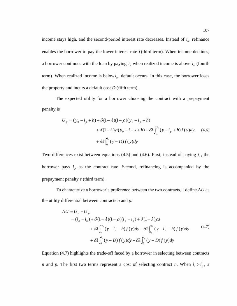
107

income stays high, and the second-period interest rate decreases. Instead of ni , refinance

enables the borrower to pay the lower interest rate i (third term). When income declines,

a borrower continues with the loan by paying ni when realized income is above ni (fourth

term). When realized income is below ni , default occurs. In this case, the borrower loses

the property and incurs a default cost D (fifth term).

The expected utility for a borrower choosing the contract with a prepayment

penalty is

p

p

i

y

ip

ppp

dyyfDy

dyyfhiyhsiy

hiyhiyU

0

0

00

)()(

)()()()1(

))(1)(1()(

0

(4.6)

Two differences exist between equations (4.5) and (4.6). First, instead of paying ni , the

borrower pays pi as the contract rate. Second, refinancing is accompanied by the

prepayment penalty s (third term).

To characterize a borrower’s preference between the two contracts, I define ΔU as

the utility differential between contracts n and p.

pn

pn

ii

y

ip

y

in

npnp

pn

dyyfDydyyfDy

dyyfhiydyyfhiy

siiii

UUU

00)()()()(

)()()()(

)1())(1)(1()(

00

(4.7)

Equation (4.7) highlights the trade-off faced by a borrower in selecting between contracts

n and p. The first two terms represent a cost of selecting contract n. When pn ii , a

108

borrower pays an interest premium by selecting contract n. Given ni is less affordable, an

additional cost associated with contract n is the increased probability of default. In return,

the borrower enjoys a greater benefit when refinancing, because no penalty needs to be

paid with a contract n. The borrower selects contract n if its benefit outweighs the cost.

To rule out the trivial outcome that contract p dominates contract n at all times, I impose

the restriction that pn iis .51

It is also clear that the utility differential increases with

ni and deceases with pi , 0/ piU and 0/ niU .

The borrower’s choice of prepayment penalty depends on his income uncertainty.

Differentiating ΔU with respect to , we have

02

))(()(2

0

0

y

iiiisiiyU pnpnpn

(4.8)

Equation (4.8) is strictly negative. This suggests that as becomes greater, contract p

becomes increasingly attractive as compared to the contract n. The intuition underlying

equation (4.8) is critical. Because reduced income level deprives the borrower of the

option to refinance, a large translates to a lower expected payoff from contract n. As a

result, the incentive to pay an interest premium to eliminate the prepayment penalty is

lessened.

51 Given pn ii , the first term is strictly negative. In addition, the third-line and fourth-line expressions of

(6) are strictly negative. Intuitively, contract p always provides greater utility when income is reduced.

When the reduction is moderate, contract p is cheaper due to pn ii . Furthermore, the lower contract rate

of contract p also reduces the probability of default. Hence, sii nl )1())(1)(1( must

be strictly positive to allow for possible coexistence of the two contracts. Otherwise, I yield a trivial

outcome that that contract p dominates contract n. Simplification yields ln iis .

109

I further characterize the borrower’s indifference curve, which is a set of ),( pn ii

that makes a borrower indifferent between contracts n and p. Setting ΔU = 0, and

implicitly differentiating ni with respect to pi , I have:

0)()1(

)()1(

000

000

yiyy

yiyy

iU

iU

i

i

n

p

n

p

p

n

(4.9)

Not surprisingly, equation (4.9) indicates that the indifference curve is upward sloping. It

reflects the simple fact that when ni increases, pi must also rise for a borrower to remain

indifferent. To determine how alters the relative position of the indifference curve, I

implicitly differentiate ni with respect to holding ΔU = 0. Equation (4.8) and

0/ niU collectively imply that 0/ ni , which suggests that a greater shifts

the indifference curve downward.

Equilibrium with Full Information

With the framework developed above, I now turn to the derivation of mortgage

market equilibria. I define an equilibrium as a set of mortgage contracts such that 1) each

borrower type makes contract choices based on utility maximization, and 2) the lender

earns nonnegative profit, and no other lenders have an incentive to enter the market by

offering contracts outside the equilibrium set.

I first consider the equilibrium under full information. Suppose there exist two

types of borrowers who are identical in all aspects except for their expected income

uncertainty. High-risk borrowers (type H) are characterized by having a greater

110

LHH , than low-risk borrowers (type L).52

Under full information, the lender’s

problem is simple. Since a borrower’s risk type is observable to the lender and the

mortgage market is competitive, the lender offers the zero-profit rates of either contract n

or p that correspond to the borrower type. To obtain the zero-profit penalty contract rates

of each borrower type, I substitute H and L , respectively, into (4.1) and (4.2) and

solve for *

ni and *

pi . 0/ n and 0/ p , respectively, implies that ** L

n

H

n ii

and ** L

p

H

p ii . Intuitively, the borrower type with a greater probability of an income

decline will be charged higher interest rates.

In reality, designating separate contracts to different borrower types may not be

feasible. First, borrowers are normally better in assessing their future income uncertainty

than the lender. Second, even when observable, lenders are prevented from using certain

borrower characteristics (e.g. age, gender, and race) to price mortgages. When the lender

is at an informational disadvantage and borrower types cannot be credibly identified, free

choice between contracts n and p must be allowed.

Equilibrium with Asymmetric Information

When there is information asymmetry, borrowers’ risk types are unobservable to

the lender. As a result, lenders are unable to offer contracts contingent on risk types. In

general, mortgage market equilibria under information asymmetry could be of two types:

a pooling equilibrium or a separating equilibrium. A pooling equilibrium is characterized

52 I define risk types based on default probability. High (low) risk indicates a greater (smaller) likelihood of

default.

111

by lenders offering a single type of contract, either with or without a prepayment penalty,

at a uniform rate to all borrowers. On the other hand, a separating equilibrium is a market

outcome in which borrowers of different risk types obtain distinct contracts. Because the

choice of prepayment penalty analyzed here is considered dichotomous, it is possible to

derive pooling equilibria from the model (Posey and Yavas, 2001). However, given the

observed coexistence of contracts with and without a prepayment penalty in the U.S.

mortgage market, I focus exclusively on the properties of a separating equilibrium that

are empirically relevant. I denote by LHjii jpn ,),,( the no-penalty rate ni that makes

a borrower of risk type j indifferent to a choice between a contract n and a contract p

charging pi .

Proposition 1. There exists a separating equilibrium where the high-risk borrowers

obtain contract p with the rate *H

pi , the low-risk borrowers obtain contract n with the rate

*L

ni , and the lenders earn zero expected profits, if and only if );(),( ***

Lpn

L

nH

H

pn iiiii .

Proof. See Appendix B

Here, I briefly discuss the underlining intuition. As shown previously, borrower

indifference curves are upward-sloping. In addition, the indifference curve of the high-

risk type lies below that of the low-risk type. Recall that 0/ ni . The parameter

conditions specified in proposition 1 ensure that the contract combination ),( ** H

p

L

n ii is

located above the indifference curve of the high-risk type but below that of the low-risk

112

type. When both *L

ni and *H

pi are offered, high-risk borrowers prefer contract p to contract

n. This can be verified by referring to figure 4.1. The vertical line passing through point

),( ** H

p

L

n ii intercepts high-risk indifference curve at the point )),;(( ** H

pH

H

pn iii . This

indicates that high-risk borrowers are indifferent between a contract p priced at *H

pi and a

contract n charging );( *

H

H

pn ii , which is cheaper than *L

ni . Thus, high-risk borrowers will

choose contract p over contract n. Turning to low-risk borrowers, the vertical line passing

through the point ),( ** H

p

L

n ii intercepts low-risk indifference curve at point

)),;(( ** H

pH

H

pn iii . This indicates that high-risk borrowers are indifferent between a

contract p priced *H

pi at and a contract n charging );( *

L

H

pn ii , which is more expansive

than *L

ni . Thus, low-risk borrowers will choose contract n over contract p.

For the separating equilibrium to be feasible, another necessary condition is that

no other lenders can make a positive profit by offering alternative contracts when

),( ** H

p

L

n ii is offered. Because both *L

ni and *H

pi yield zero-profit lending profit, it is

impossible for other lenders to offer a set of alternative separating contracts and make a

positive profit. The question becomes whether it is possible for other lenders to profit by

offering pooling contracts. First, offering a pooling no-penalty contract is infeasible. In

the presence of *L

ni , the pooling no-penalty rate *

ni is greater than *L

ni and attracts no

borrowers. Second, the parameter condition that );( **

Lpn

L

n iii ensures that a pooling

penalty contract is less preferable to low-risk borrowers than a contract n priced at *L

ni .

When simultaneously offered with ),( ** H

p

L

n ii , *

pi would only attract high-risk borrowers

113

and generate a negative profit. Because no lender has an incentive to deviate, ),( ** H

p

L

n ii is

indeed a separating equilibrium.

Does the Prohibition of Prepayment Penalties Benefit or Hurt Borrowers?

Before moving to the empirical analysis, it is important to discuss the welfare

implications of prohibiting prepayment penalties. Such a prohibition is equivalent to

imposing a pooling equilibrium in which lenders offer only contracts without a penalty

and charge the pooling no-penalty rate *

ni . Such a pooling equilibrium imposes welfare

losses on both types of borrowers.

Proposition 2. If );();( ***

Lpn

L

nH

H

pn iiiii , a forced pooling equilibrium where

contract n is offered at the rate *

ni to all borrowers is welfare-reducing as compared to the

separating equilibrium where the high-risk borrowers obtain contract p with the rate *H

pi ,

the low-risk borrowers obtain contract n with the rate *L

ni .

Proof. First, low-risk borrowers are worse off because they now pay a higher mortgage

rate, ** L

nn ii . The pooling equilibrium is also welfare-reducing to high-risk borrowers.

Because high-risk borrowers would have selected a contract with a prepayment penalty

when *L

ni is offered, it must be the case that )()( ** L

n

H

n

H

p

H

p iUiU . If prepayment penalties

are prohibited, high-risk borrowers must pay the pooling no-penalty rate *

ni , which is

even higher than *L

ni . It must be the case that )()( **

n

H

n

H

p

H

p iUiU .

114

Figure 4.1 illustrates the welfare reduction to each type of borrower caused by the

prohibition of prepayment penalties. Recall that the pooling no-penalty rate

*** )1( L

n

H

nn iii is strictly greater than *L

ni . Thus, the welfare loss to a low-risk

borrower is represented by the vertical distance between *

ni and *L

ni . Under the separating

equilibrium, a high-risk borrower would have selected contract p and paid *H

pi , which

generates the same level of utility as a contract n charging );( *

H

H

Pn ii . The welfare loss

to high-a risk borrower is represented by the vertical distance between *

ni and );( *

H

H

Pn ii .

It is also straight forward to see that the prohibition of prepayment penalties can

increase the likelihood of mortgage defaults. Because the pooling no-penalty rate *

ni is

strictly greater than *L

ni and *H

pi , the chance of having the second-period income y below

the interest payment becomes greater. Thus, a mortgage default becomes more likely. Of

course, this clear-cut implication is predicated on the assumption of constant property

prices. The occurrences of strategic defaults, which may be increased by prepayment

penalties, become relevant if that assumption is relaxed. As a result, the net effect of

prohibiting prepayment penalty on default rate is, at best, ambiguous. The model also

explains the empirical finding that the rate reduction associated with a prepayment

penalty is, in general, insufficient to compensate the value of the option to prepay.53

Because riskier borrowers tend to select loans with a prepayment penalty, the rate

reduction must be offset by a risk premium charged on this group of borrowers.

53 See Goldstein and Son (2003) and LaCour-Little and Holmes (2008).

115

Empirical Analysis

Hypothesis

Proposition 1 generates three testable predictions. First, under information

asymmetry, observationally equivalent borrowers are likely to be faced with the choice of

loans with and without a prepayment penalty. The first prediction is corroborated by the

coexistence of both types of contracts in the U.S. residential mortgage market. The

second prediction is that contracts with a prepayment penalty originate at a lower rate.

Several studies document that mortgages with a prepayment penalty are associated with

lower cost of credit, such as reduced annual percentage rates (APRs) and note rates, after

controlling for other risk factors.54

Finally, the third prediction is that riskier borrowers

choose contracts with a prepayment penalty. This prediction mirrors the standard positive

correlation between contractual choices and risk occurrences, which is the focus of most

empirical tests of adverse selection.55

The remaining part of this paper follows this

tradition and examines the link between prepayment penalty and mortgage termination

outcomes.

The information asymmetry hypothesis predicts a positive correlation between

expected default probabilities and prepayment penalty choices. Although the ex ante

default probabilities are not directly observable, given a large sample, these probabilities

can be approximated using ex post default outcomes. Thus, a positive correlation between

the choice of a prepayment penalty and default rate is consistent with the information

54 See DeMong and Burroughs (2005) and LaCour-Little and Holmes (2008).

55 See Dionne, Gouriéroux, and Vanasse (2001) for a discussion on the advantages of testing the positive

correlation as opposed to testing other predictions.

116

asymmetry hypothesis. However, inference drawn from this simple test could be

ambiguous due to an alternative explanation. Option-based mortgage pricing literature

suggests that the values of prepayment and default options are jointly determined. A

prepayment penalty, which constrains the prepayment option, tends to increase the

likelihood of default. A positive correlation between the choices of a prepayment penalty

and default rates is uninformative in distinguishing between these two effects. To identify

the direction of the causal relationship, I exploit the fact that many prepayment penalties

expire within a relatively short period of time (e.g. one, two, or three years) after loan

origination. Elevated default risk, if caused by prepayment penalties, should disappear

after the expiration. On the other hand, the intrinsic riskiness of borrower is likely to

persist beyond prepayment penalty terms. If loans with a prepayment penalty continue to

exhibit higher default rates after the expiration of penalties, the choices of prepayment

penalty must be a result of self-selection. I formulate the following hypothesis:

H1: Mortgages originated with a prepayment penalty are more likely to default as

compared to mortgages without a prepayment penalty, and this correlation persists even

after prepayment penalties expire.

Empirical support to H1 is consistent with the information asymmetry hypothesis.

Data

The primary data used for this study comes from mortgage origination and

servicing histories provided by New Century Financial Corporation. I focus on a sample

117

of first-lien 30-year fixed-rate mortgages. The full sample consists of 51,923 FRMs

originated between January 2002 and December 2005. The loan performance of this

sample is subsequently tracked until February 2007. Table 4.1 summarizes the basic

characteristics of this sample. The average loan size is $167,744 with an average loan-to-

value (LTV) ratio of 78 percent. The average note rate is 7.30 percent. Not surprisingly,

the data exhibit patterns consistent with a subprime sample. Approximately 79.72 percent

of loans contain a prepayment penalty. The average borrower’s FICO score is 624, and

30 percent of loans originated with limited or no documentation. In addition, 82 percent

of the sample originated through mortgage brokers (wholesale loans).

Examining loans with and without prepayment penalties reveals interesting

differences between these two groups. For example, loans with a prepayment penalty

have an average contract rate of 7.16 percent, which is 74 basis points lower than the

average note rate of loans without a prepayment penalty. This is consistent with the

notion that prepayment penalties are associated with lower mortgage rates. However, this

rate differential may also be attributable to the fact that borrowers who accept

prepayment penalties have a higher average FICO score than those that do not. It also

appears that loans with a prepayment penalty have a higher debt-to-income (DTI) ratio,

which suggests that borrowers who accepted a prepayment penalty tend to borrow more

against current income. In addition, a much smaller portion of loans with prepayment

penalties are originated with mortgage discount points. Finally, mortgages with

prepayment penalties are more likely to be low-doc/ no-doc loans and loans originated

through a mortgage broker.

118

Methodology

Dionne, Gouriéroux, and Vanasse (2001) suggest that empirical evidence of

adverse selection takes the form of ―conditional dependence.‖ Let us denote by D the

probabilities of mortgage defaults, by X the set of observable risk factors that affecting

mortgage termination, and by P the choice of prepayment penalty. Variable P supplies no

additional information if and only if the predicted default probabilities, D̂ , conditioned

on X and P jointly is identical to D̂ conditioned on X alone. Formally speaking, there is

no information asymmetry is absent if and only if )|(),|( XDlPXDl ), where .).,|(.l

denotes a conditional probability density function. On the other hand, conditional

dependence, which implies )|(),|( XDlPXDl , is consistent with information

asymmetry. I test the conditional dependence using two methods: a competing-risks

hazard model and a bivariate-probit model.

Competing-Risks Hazard Model

A key prediction of the model constructed in this paper is that high-risk borrowers

tend to select contracts with a prepayment penalty. Hence, a natural way to test the

conditional dependence is to regress D on both X and P, and examine if P can explain the

variation of D in the presence of X. I conduct this test by first estimating a competing-

risks hazard model following the methodology used in Ambrose and Sanders (2003).56

56 Kau, Keenan, Lyubimov, and Slawson (2010) use a similar framework to test the existence of adverse

selection in residential mortgage origination by estimating a proportional hazard model controlling for

observable borrower and loan characteristics.

119

A borrower has the option to prepay, default, or remain current for any given

period. I define mortgages that are still current at the end of the observation period as

censored. Thus, I define )3,2,1( jT j as the latent duration for each mortgage to be

terminated during the observation period by prepaying, defaulting, or remaining current

(censored). Thus, the observed duration, , is the minimum of the jT . Conditional on a

set of explanatory variables, jX , which may include static loan characteristics at the time

of loan origination as well as time-varying economic conditions, and parameters, j , the

probability density function (pdf) and cumulative density function (cdf) for jT are

));|(exp();|();|( jjjjjjjjjjjj XrIXThXTf (4.10)

);|(exp(1);|( jjjjjjjj XrIXTF (4.11)

where r is an integer variable taking values in the set {1, 2, 3} representing the three

possible outcomes, jI is the integrated hazard for outcome j:

jT

jjjjjjj XshXTI0

);|();|( (4.12)

where jh is the hazard function.

The joint distribution of the duration and outcome is

));|(exp();|();|( 0 jjjjjjjjjjj XIXhXf (4.13)

where ),,( 321 XXXX and ),,( 321 and

3

1

0

j

jII is the aggregated integrated

hazard. Thus, the conditional probability of an outcome is

3

1

);|(

);|();,|Pr(

j

jj

jj

Xh

XhXj

(4.14)

120

I assume a separate exponential hazard function for each mortgage outcome and estimate (4.14)

using multinomial logit.

Dionne, et al., (2001) note that it would be preferable to add expected contractual

choices in (4.14) in order to address potential problems of misspecification. Expected

contractual choices can be obtained by estimating the following logit model for the

choice of prepayment.

iiii XXPENALTY )'()|1Pr( (15)

Where iX is a set of borrower and loan characteristics of mortgage i observable to the

lender, and i is the standard error. Λ is the logistic cumulative distribution function.

Because the predicted choice of prepayment penalty )ˆ( iLTYAPEN is, by construction, a

function of observable variables, it must be irrelevant to information asymmetry.

Following Dionne et al., (2001), I including iLTYAPEN ˆ as a control variable.

Bivariate-Probit Model

I also perform the version of positive correlation test as proposed by Chiappori

and Salanié (2001). The test involves estimating the following bivariate-probit model

with the choices of prepayment penalties, iP , and subsequent loan performance outcomes,

iD , as the two dependent variables.

P

iiii XXP )'()|1Pr( (4.16)

D

iiii XXD )'()|1Pr( (4.17)

121

)( denotes the standard normal distribution. iX is a vector of borrower and loan

characteristics that are observable to the lender. P

i and D

i are, respectively, the

normally distributed error terms of equation (4.16) and (4.17), which have a correlation

coefficient . A significantly positive is consistent with the conditional dependence.

Sampling

Distinguishing between adverse selection and moral hazard has been a difficult

task, because a positive correlation between contractual choices and risk occurrences is

consistent with both arguments. However, the distinction is extremely important in

determining the welfare impacts of prepayment penalties. To separate adverse selection

from the confounding effect that prepayment penalties may increase the likelihood of

mortgage default, I exploit the fact that prepayment penalties often expire in a short

period of time (e.g. one, two, or three years). I first group loans that have a prepayment

penalty by the length of their penalty terms. Then, three subsamples are constructed to

compare mortgages with no penalty, respective, to loans with one, two, and three years.

Subsample 1.1 contains mortgages with no prepayment penalty and ones with an one-

year penalty; subsample 2.1 contains mortgages with no prepayment penalty and ones

with a two-year penalty, and subsample 3.1 contains mortgages with no prepayment

penalty and ones with a three-year penalty. Tests of positive correlation are conducted

using the full sample as well as the three subsamples to ensure results are consistent

across prepayment penalties with different terms.

122

I further construct three subsamples containing only loans surviving beyond

prepayment penalty expirations to identify the effect of adverse selection. Subsample 1.2

contains mortgages without a penalty and with a one-year-penalty that have survived

beyond the first year; subsample 2.2 contains mortgages without a penalty and with a

two-year-penalty that have survived beyond two years, and subsample 3.2 contains

mortgages without a penalty and with a three-year-penalty that have survived beyond

three years. The detection of positive correlations using subsamples 1.2, 2.2, and 3.2

unequivocally support the information asymmetry hypothesis. Figure 4.2 illustrates the

construction of the six subsamples.

Variables Related to Default and Prepayment Options

In the competing risks hazard model, I include factors that may impact mortgage

default and prepayment. In the contingent claim framework, the FRM contract contains a

prepayment option and a default option. A borrower minimizes the market value of his

outstanding loan via strategically exercising these two options. To capture how much the

prepayment option is ―in-the-money,‖ I include in X a variable, ΔRATE, which is defined

as

m

t

m

t

m

it

r

rrRATE

(4.18)

where m

ir is the 30-year conventional mortgage rate at the origination of loan i, and m

tr is

the 30-year conventional mortgage rate at time t. A relative increase in ΔRATE indicates

that the market interest rate has declined, and this increases the likelihood of prepayment.

123

The theoretical mortgage literature indicates that the intrinsic values of the default

and prepayment options are jointly determined. The relative position of the default option

affects borrower refinancing strategy. Specifically, declines in property values increase

the probability of default and reduce the probability of prepayment. To account for the

competing nature of default and prepayment risk, I control for contemporary loan-to-

value (LTV) ratio, CLTV , which is computed as the ratio of the market value of the loan

to the market value of the property.

As suggested by Kau et al. (1992, 1993), interest rate volatility also plays a

critical role in determining the value of the prepayment option. Hence, I account for

interest rate volatility by including the variable MORTVOL. MORTVOL is calculated as

the standard deviation of the monthly 30-year conventional mortgage rate over the

previous 24 months. I also control for housing price volatility by including the variable

HPIVOL, which is calculated as the standard deviation of the Office of Federal Housing

Enterprise Oversight (OFHEO) state-level quarterly housing price index over the

previous two years. Following Ambrose and Sanders (2003), I control for the market’s

expectation on future interest rate by including the slope of yield curve (YLDCURVE),

which is measured as the 10-year Treasury bond rate minus the 1-year Treasury bond rate.

Variables Related to Borrower and Loan Characteristics

I control for borrower and loan characteristics in both the competing-risks hazard

model and the bivariate-probit model. Affordability and credit score are commonly used

in residential mortgage underwriting to determine a borrower’s qualification. Borrowers

with greater financial resources relative to debt level and with a superior credit history

124

should be less likely to default. Hence, I include FICO score (FICO) and the debt-to-

income (DTI) ratio (DTI), which is the monthly mortgage payment as a fraction of a

borrower’s monthly income, in the regression model to respectively control for

affordability. In addition, a significant portion of loans in the sample are originated with

limited or no documentation on income and/or assets, which possibly indicates limited

financial strength. Therefore, I include a dummy variable, DOC, to denote documentation

status. Many other borrower characteristics are shown in the literature to have influence

on loan performance. For instance, Brueckner (1992) shows that older age and high

property purchase price are associated with low mobility, which leads to reduced

propensity of prepayment. To control for borrower mobility, I control for borrower’s age

(AGE) and the appraised value reported at the time of loan origination (PROPVAL).

Mortgage choices may be correlated with unobserved borrower characteristics.

Similar to the choice of prepayment penalty, other mortgage choices, such as loan-to-

value (LTV) ratio and discount points, may also convey information regarding a

borrower’s risk profile. Brueckner (2000) shows that when the costs of default (e.g.,

damage to credit history or reputation) are private information and heterogeneous across

borrowers, high-default-risk borrowers tend to choose a higher LTV ratio. Harrison et al.

(2004) derive a similar result under the scenario when information asymmetry exists on

future income uncertainty, and default cost is relatively small. However, Harrison et al.

(2004) also show that when default cost is large, riskier borrowers tend to borrow less.

On the other hand, loans originated with greater discount points should exhibit a reduced

propensity of prepayment, because paying discount points signals either low mobility

(Dunn and Spatt 1985, Chari and Jagannathan 1986, Yang 1992, Brueckner 1994, LeRoy

125

1996, and Stanton and Wallace 1998) or high transactions costs of refinancing (Pavlov

2001, and Chang and Yavas 2009). Therefore, I include in the set of control variables the

loan-to-value ratio (LTV) and discount points (DISCPT), which is a dummy variable

equal to one if the loan is originate with discount points. In addition, the benefit from

refinancing may also depend on the outstanding balance. Assuming there are fixed costs

associated with refinancing (e.g., appraisal fees, title search time, and inconvenience etc.),

refinancing a larger-sized loan usually creates a greater benefit. Hence, I control the

principal balance at origination (LOANSIZE).

Coulibaly and Li (2009) document that risk aversion plays an important role in

determining mortgage choices. It is possible that risk aversion simultaneously determines

the choice of prepayment penalty and loan performance outcomes. I employ a dummy

variable to denote whether or not a borrower is self-employed (SELFEMP) to control for

the effects of risk aversion.20 I also include a set of dummy variables to distinguish

between purchase loans versus refinance loans (REFI), loans collateralized by a primary

residence versus ones collateralized by a non-primary residence (NONPRIMRES), and

wholesale loans versus retail loans (WHOLESALE).

Finally, I control for time and geographic-related variations in both (14) and (15).

To capture seasonal market changes of mortgage origination, I include a set of indicator

variables representing the year of origination. I control for regional fixed effects by a set

of indicator variables constructed based on in which state the property is located. The set

of indicator variables controls for differences in state laws regarding mortgage default

and foreclosure (Ambrose and Pennington-Cross, 2000) and potential impacts of different

state predatory lending laws on the choice of prepayment penalty. To further control for

126

unobserved heterogeneity and to correct for any dependence among observations drawn

from the same loan, I use robust standard errors allowing for loan-level clustering when

estimate (14). Definitions of variables are summarized in table 4.2.

Results

Results of the Competing-Risk Hazard Model

Table 4.3 presents the results from a logit regression of equation (4.15). It appears

that the choice of prepayment penalties is correlated with a number of borrower and loan

characteristics. Because those characteristics are also observable to the lender, predicted

choice on prepayment penalties using those characteristics is unrelated to information

asymmetry and must be controlled for. Following Dionne, Gouriéroux, and Vanasse

(2001), I collect the predicted probability of selecting a prepayment penalty LTYAPEN ˆ ,

and use it as a control variable in the competing-risks hazard model. Table 4.4 presents

the results from the competing-risk hazard model using the full sample. After controlling

for time-varying option-related variables, observable borrower characteristics, and

LTYAPEN ˆ from estimating equation (4.15), I find that loans with a prepayment penalty

are less likely to prepay (significant at 1 percent level), but have a greater default rate

(significant at 5 percent level). The odds ratios are calculated to gauge the marginal

effects of having a prepayment penalty on loan performance. It indicates that mortgages

with a prepayment penalty are 11.9 percent less likely to prepay and 13.9 percent more

likely to default.

127

Although it is not the main focus of this paper, the estimated coefficients of

control variables exhibit patterns largely consistent with previous mortgage termination

literature. Consistent with empirical mortgage literature, I find support for the ―jointness‖

of prepayment and default option. A larger interest rate reduction )( RATE increases the

probability of prepayment (significant at 1% level). However, it fails to exhibit a

significant effect on default. Contemporary LTV (CLTV) increases the default rate and

reduces the likelihood of prepay (both significant at 1% level). As expected, the

expectation of a raising interest rate increases mortgage prepayment and reduces default

(both significant at 1% level). Turning to borrower and loan characteristics, I find loans

with a lower FICO score, high debt-to-income ratio, and limited or no documentation are

considerably more likely to default. On the other hand, loans originated with mortgage

points are less likely to prepay.

One of the limitations of the standard ―positive correlation‖ test is its inability to

distinguish adverse selection and moral hazard. As discussed previously, prepayment

penalties often expire in a relatively short period of time and examine loan performance

after the expiration date. Model 1.1 is a competing-risks hazard model estimated using

subsample 1.1. Similar to the results obtained using the full sample, loans with a

prepayment penalty are less likely to prepay (significant at 1 percent level), but those

loans fail to exhibit a greater default rate like in the results obtained using the full sample.

To examine loan performance after prepayment penalty expiration, I re-estimate the

competing-risks hazard model using subsample 1.2, which contains loans surviving

beyond their one-year penalty expiration date. Results from model 1.2 indicate that loans

with an one-year penalty continue to exhibit a lower propensity to prepay (significant at 1

128

percent level) and a higher default rate after prepayment penalties expire (significant at 5

percent level). Loans that previously had a one-year penalty appear 38.9 percent more

likely to default after prepayment penalties expire. Table 4.6 presents the results of the

competing-risks hazard model estimated using subsamples 2.1 and 2.2. Table 4.7 presents

the results of the competing-risks hazard model estimated using subsamples 3.1 and 3.2.

The results are qualitatively similar. Estimating using sample 2.1, loans with a two-year

prepayment penalty are approximately 15.8 percent less likely to prepay as compared to

no-penalty loans. However, I fail to reject the null hypothesis that these two groups of

loans are equally likely to enter default. Estimating using only loans that have survived

beyond two years, loans that previously had a two-year penalty appear 137.7 percent

more likely to default. Overall, loans with a three-year prepayment penalty are

approximately 13.5 percent less likely to prepay (significant at 1 percent level) and 14.2

percent more likely to default (significant at 10 percent level) as compared to no-penalty

loans. Using only loans survived beyond three years, I find loans that previously had a 3-

year penalty appear to be 160.7 percent more likely to default after three years

(significant at 1 percent level). In summary, the empirical results support the information

asymmetry hypothesis. Mortgages with a prior prepayment penalty continue to have a

greater default rate than the ones without a prepayment penalty.

Results of the Bivariate-Probit Model

Estimation results of the bivariate-probit model are summarized in table 4.8.

Because the main focus of this study is to test for adverse selection, the estimated

regression is of less interest. I restrict attention only to the estimated correlations of the

129

error terms. The left-hand column shows the estimated from the default model, in

which Di is defined as a dummy variable equal to one if mortgage i enters default. Using

the full sample, the estimated correlation between the error terms is 0.087, which is

significant at 1 percent level according to the likelihood ratio test. These results suggest

that after controlling for observable characteristics, borrowers who took loans with a

prepayment penalty are still more likely to default. I further estimate the bivariate-probit

model using restricted samples to compare loans with no prepayment penalty respectively

to the ones that have an one-, two-, and three-year prepayment penalty. The results are

similar, consistently appears to be significantly positive (all at 1% level). However,

this greater default risk could be due to both adverse selection and moral hazard. To rule

out the alternative explanation that prepayment penalties increase default risk, I estimate

using only mortgages survived beyond the penalty expiration date. Consistent with

previous results from the competing-risks hazard model, continues to be significantly

positive (all at 1% level). The bivariate-probit results are consistent with the presence of

adverse selection regarding the choice of prepayment penalties.

For completeness, I also estimate the prepayment model, in which iD is redefined

as a dummy variable equal to one if mortgage i is subsequently prepaid. Prepayment

penalties appear to be negatively correlated with a lower probability of prepayment. As

shown in table 4.8, are significantly negative when looking at the entire survival

period. However, I find no similar correlation when examining the subsamples of loans

that have survived beyond the penalty expiration.

130

Summary of Findings

In this Chapter, I investigate the effects of information asymmetry on borrower

choice of prepayment penalties. I construct a theoretical model to show that under

information asymmetry, there exists a separating equilibrium such that borrowers with

high (low) default risk select loans with (without) a prepayment penalty. The model

explains the empirical fact that prepayment penalties are associated with higher default

rates. To rule out the confounding predation hypothesis, I examine a sample of FRM

surviving beyond their prepayment penalty terms. Mortgages with prior prepayment

penalties are more likely to default even after prepayment penalties expire. In contrast to

the view that prepayment penalties are predatory and trigger mortgage default, this study

suggests a distinct causal relation: high default risk induces borrowers to accept

prepayment penalties. Regulations prohibiting prepayment penalties may, in fact,

increase mortgage default rates and reduce consumer welfare.

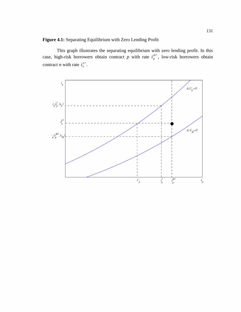
131

Figure 4.1: Separating Equilibrium with Zero Lending Profit

This graph illustrates the separating equilibrium with zero lending profit. In this

case, high-risk borrowers obtain contract p with rate *H

pi , low-risk borrowers obtain

contract n with rate *L

ni .

132

Figure 4.2: Subsample Construction

133

Table 4.1: Descriptive Statistics

This table presents the descriptive statistics of the sample. RATE is the mortgage note rate. FICO

is borrower’s credit score. DOC is a dummy variable indicating whether or not the loan was

originated with limited or no documentation of borrower’s income and/or asset (1=low-doc/no-

doc loan). AGE is borrower’s age at origination. PROPVAL is the appraised value of the property.

LOANSIZE is the total loan amount borrowed (measured in thousands of dollars). LTV is the loan-

to-value ratio. DISCPT is a dummy variable equal to 1 if the loan is originated with discount

points. SELFEMP is a dummy variable equal to 1 if the primary borrower is self-employed. REFI

is a dummy variable equal to 1 if the loan is a refinance loan. NONPRIMRES is a dummy variable

equal to 1 if the property is not the primary residence of the borrower. WHOLESALE is a dummy

variable equal to 1 if the loan is a wholesale loan.

Full Sample Without PP With PP

Mean Std. Dev. Mean Std. Dev. Mean Std. Dev. t-stat.

RATE 7.309 1.190 7.897 1.280 7.160 1.117 58.650***

FICO 623.611 63.186 604.026 61.499 628.593 62.639 -36.067***

DTI 0.220 0.090 0.197 0.086 0.225 0.091 -28.884***

DOC 0.305 0.460 0.271 0.445 0.314 0.464 -8.453***

AGE 46.077 12.009 47.278 12.008 45.771 11.991 11.510***

PROPVAL 229.203 159.321 172.206 124.004 243.703 163.989 -41.802***

LOANSIZE 167.744 105.590 128.724 87.790 177.670 107.421 -43.228***

LTV 78.029 14.670 78.082 12.715 78.015 15.127 0.418

DISCPT 0.275 0.447 0.489 0.500 0.221 0.415 56.738***

SELFEMP 0.153 0.360 0.143 0.350 0.156 0.363 -3.190***

REFI 0.846 0.361 0.887 0.317 0.835 0.371 13.124***

NONPRIMRES 0.079 0.270 0.051 0.221 0.086 0.281 -11.937***

WHOLESALE 0.830 0.375 0.713 0.452 0.860 0.347 -36.192***

# of Obs. 51,923 10,530 41,393

134

Table 4.2: Definition of Variables

VARIABLE DEFINITIONS

PENALTY Dummy variable equal to 1 if the loan has a prepayment penalty

ΔRAT E Mortgage rate reduction

CLTV Contemporary loan-to-value ratio calculated as the ratio of the market

value of the loan to the market value of the property

YLDCURVE Slope of yield curve calculated as the 10-year Treasury bond rate

minus the 1-year Treasury bond rate

MORTVOL Standard deviation of the monthly 30-year conventional mortgage rate

over the previous 24 months

HPIVOL Standard deviation of OFHEO state-level quarterly housing price index

over the previous two years

FICO Credit score of the primary borrower

DTI Debt-to-income ratio calculated as the monthly mortgage payment as a

fraction of a borrower’s monthly income

DOC Dummy variable equal to 1 if the loan is originated with limited or

no documentation

AGE Age of the primary borrower

PROPVAL Appraised value of the property

LTV Combined loan-to-value ratio at origination

DISCPT Dummy variable equal to 1 if the loan is originated with discount points

LOANSIZE Principal balance at origination

SELFEMP Dummy variable equal to 1 if the primary borrower is self-employed

REFI Dummy variable equal to 1 if the loan is a refinance loan

NONPRIMRES Dummy variable equal to 1 if the property is not the primary residence of

the borrower

WHOLESALE Dummy variable equal to 1 if the loan is a wholesale loan

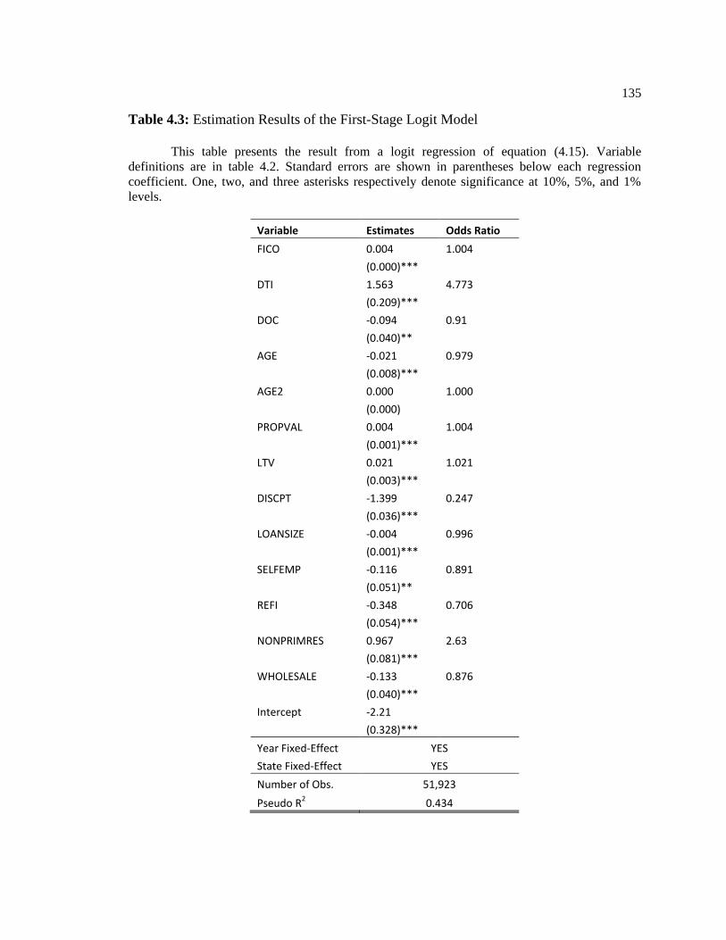
135

Table 4.3: Estimation Results of the First-Stage Logit Model

This table presents the result from a logit regression of equation (4.15). Variable

definitions are in table 4.2. Standard errors are shown in parentheses below each regression

coefficient. One, two, and three asterisks respectively denote significance at 10%, 5%, and 1%

levels.

Variable Estimates Odds Ratio

FICO 0.004 1.004

(0.000)***

DTI 1.563 4.773

(0.209)***

DOC -0.094 0.91

(0.040)**

AGE -0.021 0.979

(0.008)***

AGE2 0.000 1.000

(0.000)

PROPVAL 0.004 1.004

(0.001)***

LTV 0.021 1.021

(0.003)***

DISCPT -1.399 0.247

(0.036)***

LOANSIZE -0.004 0.996

(0.001)***

SELFEMP -0.116 0.891

(0.051)**

REFI -0.348 0.706

(0.054)***

NONPRIMRES 0.967 2.63

(0.081)***

WHOLESALE -0.133 0.876

(0.040)***

Intercept -2.21 (0.328)***

Year Fixed-Effect YES

State Fixed-Effect YES

Number of Obs. 51,923

Pseudo R2 0.434

136

Table 4.4: Results of Competing-Risks Hazard Model Using the Full Sample

This table presents the result from the competing-risk hazard model using the full sample.

It assumes a quadratic baseline hazard function. Variable definitions are in table 4.2. Robust

standard errors with loan-level clustering are shown in parentheses below each regression


levels.

Prepayment Default

Estimates Odds Ratio Estimates Odds Ratio

PENALTY -0.127 0.881 0.130 1.139

(0.019)***

(0.066)**

ΔRAT E 1.302 3.675 -0.023 0.977

(0.098)***

(0.259)

CLTV -0.588 0.555 1.213 3.365

(0.108)***

(0.330)***

YLDCURVE 0.689 1.991 -0.229 0.795

(0.009)***

(0.034)***

MORTVOL -0.926 0.396 -0.214 0.807

(0.081)***

(0.367)

HPIVOL 0.002 1.002 -0.001 0.999

(0.001)***

(0.002)

FICO -0.002 0.998 -0.009 0.991

(0.000)***

(0.000)***

DTI 0.199 1.220 1.904 6.712

(0.071)***

(0.212)***

DOC 0.077 1.081 0.446 1.562

(0.014)***

(0.044)***

AGE 0.003 1.003 -0.040 0.961

(0.003)

(0.008)***

AGE2 -0.000 1.000 0.000 1.000

(0.000)

(0.000)***

PROPVAL -0.001 0.999 -0.001 0.999

(0.000)***

(0.001)*

LTV 0.003 1.003 -0.001 0.999

(0.001)* (0.004)

137

Table 4.4: Results of Competing-Risks Hazard Model Using the Full Sample (Cont.)

This table presents the result from the competing-risk hazard model using the full sample.

It assumes a quadratic baseline hazard function. Variable definitions are in table 4.2. Robust

standard errors with loan-level clustering are shown in parentheses below each regression


levels.

Prepayment Default

Estimates Odds Ratio Estimates Odds Ratio

DISCPT -0.034 0.967 -0.169 0.845

(0.018)*

(0.059)***

LOANSIZE 0.001 1.001 -0.000 1.000

(0.000)***

(0.001)

SELFEMP -0.045 0.956 -0.045 0.956

(0.018)**

(0.056)

REFI -0.006 0.994 -0.160 0.852

(0.017)

(0.053)***

NONPRIMRES -0.050 0.951 0.098 1.103

(0.022)**

(0.071)

WHOLESALE -0.049 0.952 -0.046 0.955

(0.017)***

(0.058)

PENÂLTY 0.525 1.691 -0.007 0.993

(0.071)***

(0.224)

month -0.037 0.964 0.044 1.045

(0.003)***

(0.007)***

month2 0.000 1.000 0.000 1.000

(0.000)

(0.000)

Intercept -2.674

0.473 (0.120)*** (0.385)

Year Fixed-Effect YES

State Fixed-Effect YES

Number of Obs. 565,358

Pseudo R2 0.090

138

Table 4.3: Results of Competing-Risk Hazard Model Using Subsamples 1.1 and 1.2

MODEL 1.1 MODEL 1.2

Prepayment Default Prepayment Default

Estimates Odds Ratio Estimates Odds Ratio Estimates Odds Ratio Estimates Odds Ratio

PENALTY -0.158 0.854 0.162 1.176 -0.367 0.693 0.328 1.389

(0.032)***

(0.120)

(0.085)***

(0.158)**

ΔRATE 1.665 5.284 -0.627 0.534 -1.225 0.294 0.178 1.194

(0.186)***

(0.562)

(0.446)***

(0.707)

CLTV -0.168 0.845 2.255 9.536 0.778 2.177 2.234 9.335

(0.246)

(0.663)***

(0.630)

(0.890)**

YLDCURVE 0.697 2.007 -0.172 0.842 0.043 1.044 -0.086 0.917

(0.017)***

(0.062)***

(0.050)

(0.080)

MORTVOL 0.315 1.371 -0.765 0.465 -0.095 0.910 2.634 13.932

(0.159)**

(0.705)

(0.666)

(0.974)***

HPIVOL 0.005 1.005 0.004 1.004 0.021 1.021 0.006 1.006

(0.002)***

(0.005)

(0.004)***

(0.006)

FICO -0.002 0.998 -0.010 0.990 -0.003 0.997 -0.008 0.992

(0.000)***

(0.001)***

(0.001)***

(0.001)***

DTI 0.051 1.052 2.109 8.237 1.997 7.369 1.663 5.277

(0.147)

(0.466)***

(0.372)***

(0.600)***

DOC 0.065 1.067 0.558 1.748 0.203 1.225 0.554 1.741

(0.026)**

(0.090)***

(0.071)***

(0.111)***

AGE 0.006 1.006 -0.033 0.968 0.015 1.015 -0.018 0.982

(0.006)

(0.018)*

(0.016)

(0.023)

AGE2 -0.000 1.000 0.000 1.000 -0.000 1.000 0.000 1.000

(0.000)

(0.000)

(0.000)

(0.000)

PROPVAL -0.001 0.999 0.001 1.001 -0.003 0.997 0.001 1.001

(0.001)*

(0.000)**

(0.001)**

(0.000)*

LTV -0.002 0.998 -0.000 1.000 -0.010 0.991 0.000 1.000

(0.003) (0.006) (0.007) (0.008)

139

Table 4.3: Results of Competing-Risk Hazard Model Using Subsamples 1.1 and 1.2 (Cont.)

MODEL 1.1 MODEL 1.2



DISCPT 0.188 1.207 -0.585 0.557 -0.348 0.706 -0.545 0.580

(0.050)***

(0.185)***

(0.132)***

(0.223)**

LOANSIZE 0.001 1.001 -0.003 0.997 0.004 1.004 -0.003 0.997

(0.001)*

(0.001)***

(0.001)***

(0.001)***

SELFEMP 0.008 1.008 -0.139 0.870 -0.082 0.921 -0.191 0.826

(0.034)

(0.117)

(0.096)

(0.146)

REFI 0.026 1.026 -0.276 0.759 -0.175 0.839 -0.237 0.789

(0.035)

(0.126)**

(0.095)*

(0.165)

NONPRIMRES -0.071 0.931 0.173 1.189 0.215 1.240 -0.040 0.961

(0.050)

(0.191)

(0.125)*

(0.244)

WHOLESALE 0.004 1.004 -0.011 0.989 -0.109 0.897 -0.021 0.980

(0.031)

(0.100)

(0.090)

(0.130)

PENÂLTY 1.069 2.913 -1.495 0.224 -0.475 0.622 -1.561 0.210

(0.169)***

(0.542)***

(0.422)

(0.670)**

month -0.009 0.991 0.088 1.092 0.348 1.416 0.220 1.246

(0.005)*

(0.013)***

(0.019)***

(0.019)***

month2 -0.001 0.999 -0.001 0.999 -0.007 0.993 -0.003 0.997

(0.000)***

(0.000)***

(0.000)***

(0.000)***

Intercept -2.999

0.474

-6.641

-3.454 (0.256)*** (0.744) (0.714)*** (0.931)***

Year Fixed-Effect YES YES

State Fixed-Effect YES YES

Number of Obs. 156,167 116,433

Pseudo R2 0.100 0.192

140


MODEL 2.1 MODEL 2.2


Estimates Odds Ratio Estimates

Odds Ratio Estimates


Odds Ratio

PENALTY -0.171 0.842 -0.051 0.951 0.229 1.258 0.866 2.377

(0.043)***

(0.154)

(0.245)

(0.338)**

ΔRATE 2.121 8.335 -1.022 0.360 -1.890 0.151 -0.993 0.371

(0.199)***

(0.595)*

(0.855)**

(1.022)

CLTV -0.206 0.814 1.092 2.981 0.711 2.036 0.937 2.553

(0.250)

(0.769)

(1.563)

(2.339)

YLDCURVE 0.703 2.021 -0.194 0.823 0.069 1.071 -0.324 0.724

(0.018)***

(0.066)***

(0.118)

(0.183)*

MORTVOL 0.437 1.548 -0.121 0.886 0.134 1.143 5.692 296.603

(0.171)**

(0.727)

(1.508)

(2.100)***

HPIVOL 0.007 1.007 0.001 1.001 0.008 1.008 -0.013 0.987

(0.002)***

(0.005)

(0.009)

(0.015)

FICO -0.002 0.998 -0.009 0.991 -0.003 0.997 -0.007 0.993

(0.000)***

(0.001)***

(0.001)***

(0.001)***

DTI -0.058 0.944 1.902 6.700 0.029 1.030 0.531 1.700

(0.157)

(0.490)***

(0.835)

(1.087)

DOC 0.098 1.103 0.459 1.583 0.246 1.279 0.586 1.796

(0.030)***

(0.102)***

(0.142)*

(0.187)***

AGE 0.005 1.005 -0.030 0.971 0.016 1.016 -0.038 0.963

(0.006)

(0.019)

(0.032)

(0.036)

AGE2 -0.000 1.000 0.000 1.000 -0.000 1.000 0.000 1.000

(0.000)

(0.000)

(0.000)

(0.000)

PROPVAL -0.001 0.999 -0.002 0.998 -0.001 0.999 -0.007 0.993

(0.000)***

(0.002)

(0.003)

(0.003)*

LTV -0.003 0.997 0.003 1.003 -0.004 0.996 -0.013 0.987

(0.003) (0.009) (0.017) (0.023)

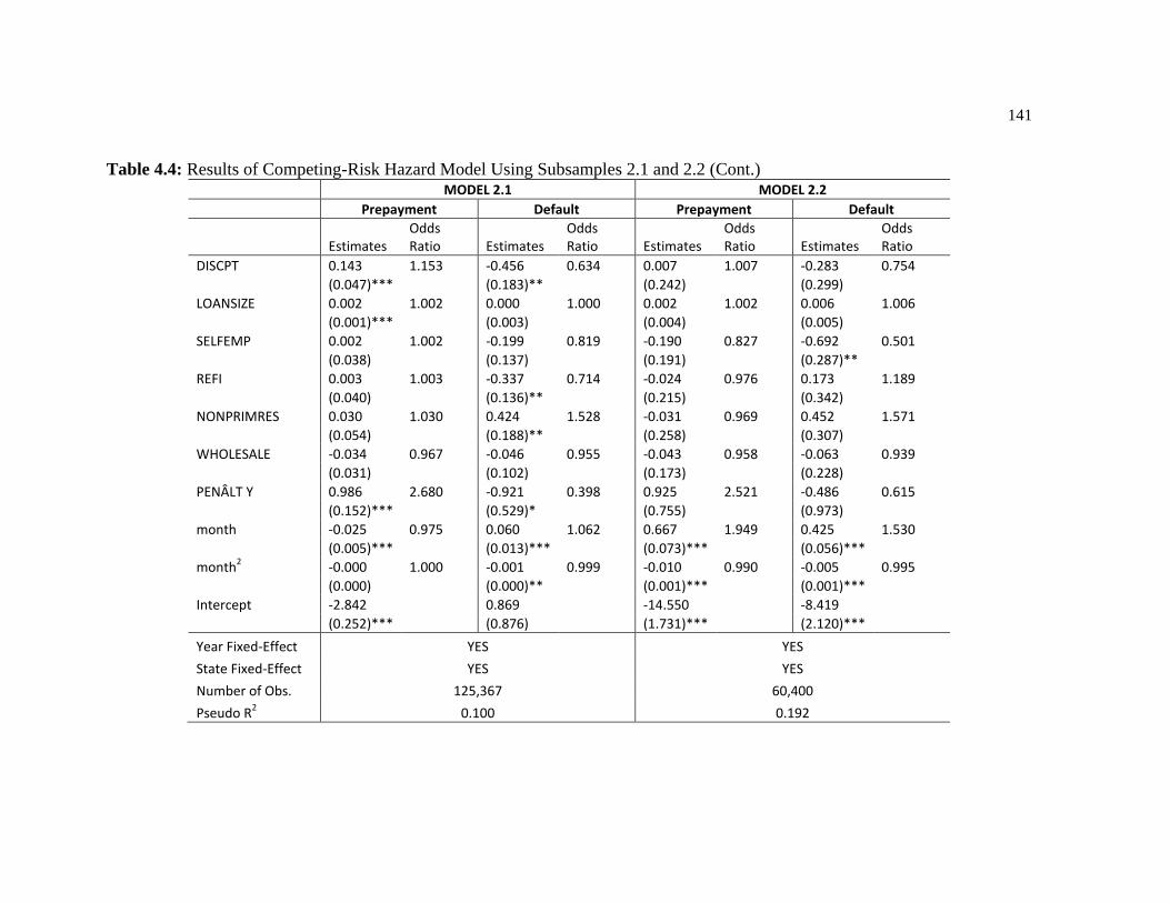
141

Table 4.4: Results of Competing-Risk Hazard Model Using Subsamples 2.1 and 2.2 (Cont.) MODEL 2.1 MODEL 2.2





Odds Ratio

DISCPT 0.143 1.153 -0.456 0.634 0.007 1.007 -0.283 0.754

(0.047)***

(0.183)**

(0.242)

(0.299)

LOANSIZE 0.002 1.002 0.000 1.000 0.002 1.002 0.006 1.006

(0.001)***

(0.003)

(0.004)

(0.005)

SELFEMP 0.002 1.002 -0.199 0.819 -0.190 0.827 -0.692 0.501

(0.038)

(0.137)

(0.191)

(0.287)**

REFI 0.003 1.003 -0.337 0.714 -0.024 0.976 0.173 1.189

(0.040)

(0.136)**

(0.215)

(0.342)

NONPRIMRES 0.030 1.030 0.424 1.528 -0.031 0.969 0.452 1.571

(0.054)

(0.188)**

(0.258)

(0.307)

WHOLESALE -0.034 0.967 -0.046 0.955 -0.043 0.958 -0.063 0.939

(0.031)

(0.102)

(0.173)

(0.228)

PENÂLT Y 0.986 2.680 -0.921 0.398 0.925 2.521 -0.486 0.615

(0.152)***

(0.529)*

(0.755)

(0.973)

month -0.025 0.975 0.060 1.062 0.667 1.949 0.425 1.530

(0.005)***

(0.013)***

(0.073)***

(0.056)***

month2 -0.000 1.000 -0.001 0.999 -0.010 0.990 -0.005 0.995

(0.000)

(0.000)**

(0.001)***

(0.001)***

Intercept -2.842

0.869

-14.550

-8.419 (0.252)*** (0.876) (1.731)*** (2.120)***



Number of Obs. 125,367 60,400

Pseudo R2 0.100 0.192

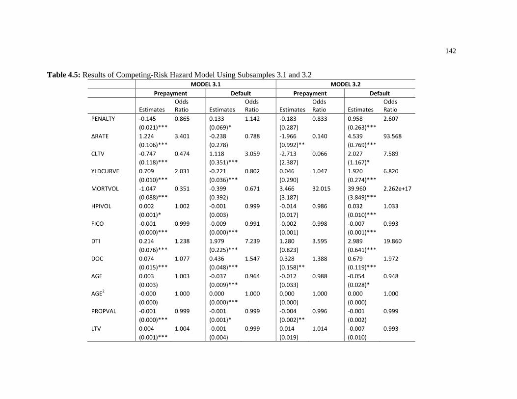
142


MODEL 3.1 MODEL 3.2





Odds Ratio

PENALTY -0.145 0.865 0.133 1.142 -0.183 0.833 0.958 2.607

(0.021)***

(0.069)*

(0.287)

(0.263)***

ΔRATE 1.224 3.401 -0.238 0.788 -1.966 0.140 4.539 93.568

(0.106)***

(0.278)

(0.992)**

(0.769)***

CLTV -0.747 0.474 1.118 3.059 -2.713 0.066 2.027 7.589

(0.118)***

(0.351)***

(2.387)

(1.167)*

YLDCURVE 0.709 2.031 -0.221 0.802 0.046 1.047 1.920 6.820

(0.010)***

(0.036)***

(0.290)

(0.274)***

MORTVOL -1.047 0.351 -0.399 0.671 3.466 32.015 39.960 2.262e+17

(0.088)***

(0.392)

(3.187)

(3.849)***

HPIVOL 0.002 1.002 -0.001 0.999 -0.014 0.986 0.032 1.033

(0.001)*

(0.003)

(0.017)

(0.010)***

FICO -0.001 0.999 -0.009 0.991 -0.002 0.998 -0.007 0.993

(0.000)***

(0.000)***

(0.001)

(0.001)***

DTI 0.214 1.238 1.979 7.239 1.280 3.595 2.989 19.860

(0.076)***

(0.225)***

(0.823)

(0.641)***

DOC 0.074 1.077 0.436 1.547 0.328 1.388 0.679 1.972

(0.015)***

(0.048)***

(0.158)**

(0.119)***

AGE 0.003 1.003 -0.037 0.964 -0.012 0.988 -0.054 0.948

(0.003)

(0.009)***

(0.033)

(0.028)*

AGE2 -0.000 1.000 0.000 1.000 0.000 1.000 0.000 1.000

(0.000)

(0.000)***

(0.000)

(0.000)

PROPVAL -0.001 0.999 -0.001 0.999 -0.004 0.996 -0.001 0.999

(0.000)***

(0.001)*

(0.002)**

(0.002)

LTV 0.004 1.004 -0.001 0.999 0.014 1.014 -0.007 0.993

(0.001)*** (0.004) (0.019) (0.010)

143

Table 4.5: Results of Competing-Risk Hazard Model Using Subsamples 3.1 and 3.2 (Cont.)

MODEL 3.1 MODEL 3.2



DISCPT -0.046 0.955 -0.171 0.843 -0.523 0.593 0.003 1.003

(0.019)**

(0.062)*** (0.245)**

(0.160)

LOANSIZE 0.001 1.001 -0.000 1.000 0.005 1.005 -0.001 0.999

(0.000)***

(0.001) (0.002)**

(0.003)

SELFEMP -0.042 0.959 -0.018 0.982 -0.135 0.874 -0.064 0.938

(0.019)**

(0.060) (0.199)

(0.148)

REFI -0.016 0.984 -0.148 0.862 -0.286 0.751 -0.013 0.987

(0.019)

(0.057)*** (0.185)

(0.160)

NONPRIMRES -0.050 0.952 0.092 1.096 0.200 1.221 -0.210 0.811

(0.024)**

(0.076) (0.225)

(0.219)

WHOLESALE -0.060 0.942 -0.032 0.968 -0.057 0.944 -0.370 0.691

(0.018)***

(0.060) (0.271)

(0.205)*

PENÂLTY 0.541 1.718 -0.043 0.958 -0.068 0.935 0.177 1.194

(0.075)***

(0.239) (0.872)

(0.823)

month -0.034 0.966 0.048 1.049 1.885 6.589 2.349 10.470

(0.003)***

(0.007)*** (0.302)***

(0.321)***

month2 0.000 1.000 -0.000 1.000 -0.022 0.978 -0.026 0.974

(0.000)

(0.000) (0.004)***

(0.004)***

Intercept -2.724

0.518 -42.503

-56.177

(0.127)***

(0.408) (5.927)***

(6.830)***



Number of Obs. 487,670 107,053

Pseudo R2 0.092 0.353

144

Table 4.6: Results of Bivariate-Probit Models

This table presents the estimated correlations, , of the error terms estimated from equations (4.16) and (4.17), which are jointly

estimated as a bivariate-probit model. The standard error of and the 2 statistic of the LM test ( = 0) are also provided. One, two, and

three asterisks respectively denote significance at 10%, 5%, and 1% levels.

Default Model Prepayment Model

Estimates Standard

Error

LR test: =

0

Estimates Standard

Error

LR test: =

0

Full Sample 0.087*** 0.017 27.279 -0.090*** 0.012 51.742

Subsample 1.1 0.089*** 0.029 9.279 -0.068*** 0.021 10.569

Subsample 1.2 0.140*** 0.045 9.579 -0.048 0.034 1.990

Subsample 2.1 0.113*** 0.036 9.917 -0.100** 0.028 12.431

Subsample 2.2 0.289*** 0.083 10.706 0.099 0.077 1.613

Subsample 3.1 0.093*** 0.018 27.146 -0.112*** 0.014 66.853

Subsample 3.2 0.362*** 0.078 17.818 -0.017 0.081 0.046

145

Chapter 5

Concluding Remarks

This dissertation shows that understanding the screening functions of mortgage

instruments when borrowers are heterogeneous in multiple risk dimensions is not only

theoretically interesting but also possesses significant practical importance. Chapter 2

contributes to the theoretical literature on screening and signaling by pointing out that

one outcome of the conflicting role of the prepayment penalty in screening prepayment

and default risk is the possibility of a pooling equilibrium. If the negative correlation

between prepayment penalty and prepayment risk is completely offset by the positive

correlation between prepayment penalty and default risk, then all borrower types would

have identical preferences over contract choices; hence, the prepayment penalty choice of

the borrower would have no informational value to the lender about that borrower’s

prepayment or default risk. This gives rise to a pooling equilibrium as the unique

outcome. Proposition 3 characterizes the conditions under which such an equilibrium

outcome emerges. Proposition 4 states that a pooling equilibrium can exist even if the

two opposing screening roles of prepayment penalty for prepayment and default risk do

not completely offset each other—that is, even if different borrower types will prefer

different mortgage contracts. This possibility arises when there is a contract that yields

the same expected profits to the lenders, regardless of the borrower’s type that chooses

that contract. Proposition 4 states the conditions under which and when such contracts

exist, it becomes the pooling equilibrium contract. As stated above, what is interesting

about this pooling equilibrium is that it is inferior to the first-best contract of both types.

146

This is in contrast to a typical pooling equilibrium, in which only one borrower type

receives less utility than her first-best contract, while the other borrower type receives the

same utility as her first-best contract.

The contribution of the chapter 3 is threefold. First, it shows that the

heterogeneity of transaction costs can explain the commonly observed practice of lenders

offering a menu of loans with a wide range of points-coupon combinations. The study

compliments existing mortgage-choice literature by supplying an alternative theory on

why people choose to pay points. Second, the study finds empirical support for the

transaction-costs theory, by using a new measure that isolates the effect of transaction

costs from that of mobility. This new measure focuses on the extent that borrowers

overpay in terms of mortgage rate. A borrower may overpay for his mortgage due to

either high transaction cost (e.g. cost of search and bargaining) or limited expected

holding period. While the high transaction cost often correlates with a reduced tendency

of prepayment, shorter expected holding period implies exactly the opposite. Thus, if the

―overvaluedness‖ of a mortgage loan is negatively correlated with the probability of

prepayment, it is highly likely caused by high transaction cost rather than high mobility. I

support the validity of this measure by showing that borrowers with overvalued loans are

less likely to prepay. In particular, these loans are less responsive to declining interest

rates. Finally, to the knowledge, this is the first study examining the relation between the

signaling role of discount points and mortgage securitization. The unique dataset enables

us to study the originator’s interpretation of borrowers paying discount points. I show that

mortgage originators employ a points-coupon menu to sort loans based on transaction

147

costs, and mortgages held by high-cost borrowers are more likely to be retained by the

originator.

Chapter 4 reconsiders the popular predation view on subprime lending products

by examining borrowers’ choice of prepayment penalties under information asymmetry. I

show that there exists a separating equilibrium such that borrowers with high default risk

select mortgage contracts with a prepayment penalty and receive a low contract rate, and

vice versa. Thus, the positive correlation between prepayment penalties and mortgage

delinquencies, defaults, and foreclosures does not necessarily imply that prepayment

penalties elevate default risk. It may simply reflect the fact that borrowers who are

intrinsically riskier tend to select loans with a prepayment penalty. In addition, the third

essay confronts a challenge usually encountered by empirical tests of information

asymmetry: separating moral hazard from adverse selection. The study exploits the fact

that loan performance remains observable after prepayment penalties expire. To rule out

the potential causal effect of prepayment penalties on loan performance, I focus on loan

terminations in time periods when prepayment penalties are no longer effective.

Empirical evidence supports the adverse selection hypothesis.

This dissertation also answers two important questions asked at the beginning of

this dissertation. First, how do different borrowers risk dimensions interact with each

other and why are those interactions important? The first essay shows that default and

prepayment risks may offset each other and generate pooling equilibria that compromise

the screening function of certain mortgage instruments. This outcome does not exist

when default risk or prepayment risk is considered separately. The second essay shows

that prepayment risk may be further separated into mobility and transactions costs.

148

Although both are sources of greater likelihood of prepayment, lenders may not treat both

with equal importance. Finally, the third essay points out a potential linkage between

prepayment and default risks. When borrower income is commonly used in underwriting

for determining a borrower’s qualification, default and prepayment risks are tied together.

Compromised financial strength not only may trigger default but also may increase the

probability that a borrower is ineligible for a new loan. The choice of prepayment penalty

reflects this linkage and has important policy implications.

The second question addressed by this dissertation is that: Does allowing a

greater variety of mortgage choices benefit consumers? Based on the work here, the

answer is positive. The first essay shows that a single instrument (e.g. prepayment

penalty) is insufficient to screen two risk dimensions. Allowing for the simultaneous use

of more instruments may potentially mitigate this problem. The third essay indicates that

eliminating the choice of prepayment penalty is equivalent to forcing an inefficient

pooling equilibrium. The social welfare and consumer welfare are both reduced by the

prohibition of prepayment penalties. In summary, the studies here suggest that a greater

variety of mortgage products is desirable and should be promoted.

149

BIBLIOGRAPHY

Agarwal, S., J. Driscoll, X. Gabaix, and D. Laibson. (2007). The Age of Reason:

Financial Decisions Over the Lifecycle. Unpublished manuscript.

Agarwal, S, B. W. Ambrose, S. Chomsisengphet, and A. B. Sanders. (2011) Thy Neighbor’s

Mortgage: Does Living in a Subprime Neighborhood Effect One’s Probability of

Default? Real Estate Economics (Forthcoming).

Ambrose, B. W., and R. J. Buttimer, Jr. (2000). Embedded Options in the Mortgage

Contract. The Journal of Real Estate Finance and Economics 21:2 95-111.

Ambrose, B. W., M. LaCour-Little, and A. Sanders. (2005). Does Regulatory Capital

Arbitrage, Reputation, or Information Asymmetry Drive Securitization? Journal of

Financial Services Research 28.1/2: 113-133.

Ambrose, B. W., M. LaCour-Little, and A. Sanders. (2004). The Effect of Conforming

Loan Status on Mortgage Yield Spreads: A Loan Level Analysis. Real Estate

Economics 32.4: 541-569.

Ambrose, B. W., and A. Pennington-Cross. (2000) Local Economic Risk Factors and the

Primary and Secondary Mortgage Markets. Regional Science and Urban Economics

30.6: 683-701.

Ambrose, B. W., and A. Sanders. (2003) Commercial Mortgage Backed Securities:

Prepayment and Default. Journal of Real Estate Finance and Economics 26.2/3:

175-192.

Archer, W. R., D. C. Ling, and G. A. McGill. (1996). The Effect of Income and

Collateral Constraints on Residential Mortgage Terminations. Regional Science and

Urban Economics 26.3,4: 235-261.

Basmann, R. L., (1960). On Finite Sample Distributions of Generalized Classical Linear

Identifiability Test Statistics. Journal of the American Statisical Association 55.292:

650-59.

Ben-Shahar, D., (2006). Screening Mortgage Default Risk: A Unified Theoretical

Framework. Journal of Real Estate Research 28(3): 215-239.

Bucks, B., and K. Pence. (2008). Do Borrowers Know Their Mortgage Terms? Journal of

Urban Economics 64.2: 218-233.

Brown, J. R., and A. Goolsbee. (2002). Does the Internet Make Markets More

Competitive? Evidence from the Life Insurance Industry. Journal of Political

Economy 110.3: 481-507.

http://www.personal.psu.edu/bwa10/workingpapers/alt4_REE.pdf



150

Brueckner, J. K. (1992). Borrower Mobility, Self-Selection, and the Relative Prices of

Fixed- and Adjustable-Rate Mortgages. Journal of Financial Intermediation 2, 401-

421.

Brueckner, J. K. (1994). Borrower Mobility, Adverse Selection, and Mortgage

Points.‖Journal of Financial Intermediation 3: 416-441.

Brueckner, J. K. (2000). Mortgage Default with Asymmetric Information. Journal of

Real Estate Finance and Economics 20.3: 251-274.

Calem, P. S., and M. LaCour-Little. (2004) Risk-Based Capital Requirements for

Mortgage Loans. The Journal of Banking and Finance 28: 647-672.

Calem, P. S. and S. M. Wachter. (1999). Community Reinvestment and Credit Risk:

Evidence from an Affordable Home Loan Program. Real Estate Economics 27: 105-

134.

Carlin, B. (2009). Strategic Price Complexity in Retail Financial Markets. Journal of

Financial Economics 91:278.

Campbell, J, Y. (2006) Household Finance. Journal of Finance 61:1553-1604.

Campbell, J. Y., S. Giglio, and P. Pathak. (2009). ―Forced Sales and House Prices.‖

NBER Working Paper 14866.

Chang, Y., and A. Yavas. (2009). "Do Borrowers Make Rational Choices on Points and

Refinancing?" Real Estate Economics 37.4: 635-658.

Chari, V. V., and R. Jagannathan. (1989). ―Adverse Selection in a Model of Real Estate

Lending.‖ Journal of Finance 44: 499-508.

Chiappori, P., and B. Salanié. (2000). Testing for Asymmetric Information in Insurance

Market. Journal of Political Economics 108.1: 56-78.

Chomsisengphet, S., and A. Pennington-Cross. (2006). The Evolution of the Subprime

Mortgage Market. Federal Reserve Bank of St. Louis Review 88.1: 31-56.

Cohen, A. (2005). Asymmetric Information and Learning in the Automobile Insurance

Market. Review of Economics and Statistics 87: 197-207.

Cutler, D., and R. Zeckhauser. (2000). The Anatomy of Health Insurance, in The

Handbook of Health Economics, A. J. Culyer and J. P. Newhouse, editors.

151

Danis, M., and A. Penninglon-Cross. (2008). The Delinquency of Subprime Mortgages.

Journal of Economics and Business 60.1/2: 67-90.

Deng, Y., J. M. Quigley, and R. Van Order. (1996). ―Mortgage Default and Low Down-

Payment Loans: The Cost of Public Subsidy.‖ Regional Science and Urban

Economics 26: 263-285.

Christelis, D., J. Tullio, and M. Padula. (2006). Cognitive Abilities and Portfolio Choice.

Working paper No. 5735, CEPR.

DeMarzo, P. M., and D. Duffie. (1999) A Liquidity-Based Model of Security Design.

Econometrica 67.1: 65-99.

DeMong, R. F., and J. E. Burroughs. (2005). Prepayment Fees Lead to Lower Interest

Rates. Unpublished manuscript. University of Virginia, McIntire School of

Commerce.

Dionne, G., C. Gouriéroux, and C. Vanasse (2001). Testing for Evidence of Adverse

Selection in the Automobile Insurance Market: A Comment. Journal of Political

Economy 109.2: 444-451.

Dunn, K. B., and J. J. McConnell. (1981) Valuation of GNMA Mortgage-Backed

Securities. Journal of Finance 36.3, 599-616.

Dunn, K. B., and C. S. Spatt. (1985). ―An Analysis of Mortgage Contracting: Prepayment

Penalties and the Due-on-Sale Clause.‖ Journal of Finance 40: 293-308.

Elliehausen, G., M. E. Staten, and J. Steinbuks. (2008). ―The Effect of Prepayment

Penalties on the Pricing of Subprime Mortgages.‖ Journal of Business and Economics

60: 33-46.

Finkelstein, A., and J. Poterba. (2002). Selection Effects in the Market for Individual

Annuities: New Evidence from the United Kingdom. Economic Journal 112: 28-50.

Foster, C., and R. Van Order. (1985). ―FHA Terminations: A Prelude to Rational

Mortgage Pricing.‖ Real Estate Economics 13.3, 273-291.

Goldstein, D. and S. Son. (2003). Why Prepayment Penalties Are Abusive in Subprime

Home Loans. Policy Paper No. 4. Durham, NC: Center for Responsible Lending.

Harrison D. M., T. G. Noordewier, and A. Yavas. (2004). ―Do Riskier Borrowers Borrow

More?‖ Real Estate Economics 32(3), 385-411.

152

Hogarth, J., and M. Hilgert. (2002). Financial Knowledge, Experience and Learning

Preferences: Preliminary Results from a New Survey on Financial Literacy.

Consumer Interests Annual 48.

Jackson, H.E. and L. Burlingame. (2007). Kickbacks or Compensation: The Case of

Yield Spread Premiums. Stanford Journal of Law Business and Finance 12: 289-350.

Kau J. B., and D. C. Keenan (1987). Tax, Points and Rationality in the Mortgage Market.

Journal of the American Real Estate and Urban Economics Association 15.3: 168-

184.

Kau, J. B., D. C. Keenan, W. J. Muller, and J. F. Epperson. (1992). ―A Generalized

Valuation Model for Fixed-Rate Residential Mortgages.‖ Journal of Money, Credit

and Banking 24.3: 279-299.

Kau, J. B., D. C. Keenan, W. J. Mueller, and J. Epperson. (1993). Option Theory and

Floating-Rate with a Comparison of Adjustable- and Fixed- Rate Mortgages. Journal

of Business 66.4: 595-618.

Kau, J. B., D. C. Keenan, W. J. Muller, and J. F. Epperson. (1995). ―The Valuation at

Origination of Fixed Rate Mortgages with Default and Pre-payment.‖ Journal of Real

Estate Finance and Economics 11.1: 5-36.

Korniotis, G., and A. Kumar. (2008a). Do Older Investors Make Better Investment

Decisions? Unpublished manuscript, University of Texas.

Korniotis, G., and A. Kumar. (2008b). Superior Information or a Psychological Bias? A

Unified Framework with Cognitive Abilities Resolves Three Puzzles. Unpublished

manuscript, University of Texas.

LaCour-Little, M. and S. Malpezzi. (2003). Appraisal Quality and Residential Mortgage

Default: Evidence from Alaska. Journal of Real Estate Finance and Economics 27.2:

211-233.

LaCour-Little, M. (2009). The Pricing of Mortgages by Brokers: An Agency Problem?

The Journal of Real Estate Research 31.2: 235-264.

LaCour-Little, M., and C. Holmes. (2008). ―Prepayment Penalties in Residential

Mortgage Contracts: A Cost-Benefit Analysis.‖ Housing Policy Debate 19.4, 631-

673.

Lambson, V.E., G.R. McQueen and B.A. Slade. (2004). Do Out-of-State Buyers Pay

More for Real Estate? An Examination of Anchoring-Induced Bias and Search Costs.

Real Estate Economics 32(1): 85-126.

153

LeRoy, S. F. (1996). ―Mortgage Valuation under Optimal Prepayment.‖ Review of

Financial Studies 9, 817-844.

Lin, Z., E. Rosenblatt., and V. W. Yao. (2009). Spillover Effects of Foreclosures on

Neighborhood Property Values. Journal of Real Estate Finance and Economics 38.4:

387-407.

Ling, D., and W. R. Archer. (2005) Real Estate Principles: A Value Approach. McGraw-

Hill/Irwin.

Lusardi, A., and O. Mitchell. (2007). Baby Boomer Retirement Security: The Roles of

Planning, Financial Literacy, and Housing Wealth. Journal of Monetary Economics

54: 205-224.

Lusardi, A., and P. Tufano. (2008). Debt Literacy, Financial Experience, and

Overindebtedness. Unpublished manuscript, Harvard Business School.

Mayers, C., T. Piskorski, and A. Tchistyi. (2009). The Inefficiency of Refinancing: Why

Prepayment Penalties Are Good for Risky Borrowers. Unpublished manuscript.

Columbia University and University of California, Berkeley.

Merton, R. C. (1974). On the Pricing of Corporate Debt: The Risk Structure of Interest

Rates. Journal of Finance 29.2: 449-470.

Myer, N., L. He and J. Webb. (1992). Sell-Offs of U.S. Real Estate: The Effect of

Domestic Versus Foreign Buyers on Shareholder Wealth. AREUEA Journal 20.3:

487-500.

Noordewier, T.G., D.M. Harrison and K. Ramagopal. (2001). Semivariance of Property

Value Estimates as a Determinant of Default Risk. Real Estate Economics 29.1: 127-

159.

Ong, S. E., P. H. Neo and A. C. Spieler (2006). Price Premium and Foreclosure Risk.

Real Estate Economics 34: 211-242.

Pavlov, A. D. (2001). Competing Risks of Mortgage Termination: Who Refinances, Who

Moves, and Who Defaults? Journal of Real Estate Finance and Economics 23.2: 185-

211.

Posey, L. L., and A. Yavas. (2001). ―Adjustable and Fixed Rate Mortgages as a

Screening Mechanism for Default Risk.‖ Journal of Urban Economics 49: 54-79.

Quercia, R. G., M. A. Stegman, and W. R. Davis. (2007). The Impact of Predatory Loan

Terms on Subprime Foreclosures: The Special Case of Prepayment Penalties and

Balloon Payments. Housing Policy Debate 18.2: 311-46.

154

Robins, E. H., and J. D. Schatzberg. (1986). Callable Bonds: A Risk-reducing Signaling

Mechanism, Journal of Finance 41: 935-949.

Rothschild, M., and J. E. Stiglitz. (1976). ―Equilibrium in Competitive Insurance

Markets: An Essay in the Economics of Imperfect Information.‖ Quarterly Journal of


Sargan, J.D. (1958). The Estimation of Economic Relationships Using Instrumental

Variables. Econometrica 26: 393-415.

Schuetz, J., V. Been, and I.G. Ellen. (2008). Neighborhood Effects of Concentrated

Mortgage Foreclosures. Journal of Housing Economics 17.4: 306-319.

Schwartz, E. S., and W. N. Torous. (1993). ―Mortgage Prepayment and Default

Decisions: a Poisson Regression Approach.‖ Journal of the American Real Estate and

Urban Economics Association 21.4: 431-449.

Standard & Poor’s. (2004). Trends in U.S. Residential Mortgage Products. World Wide.

http://www.standardandpoors.com (accessed March 2, 2010).

Stanton, R., and N. Wallace. (1998). ―Mortgage Choice: What’s the Point.‖ Real Estate


Stock, J. H., and Yogo, M. (2001). Testing for Weak Instruments in Linear IV Regression.

unpublished manuscript, Harvard University.

Titman, S., and W. N. Torous. (1989). ―Valuing Commercial Mortgages: An Empirical

Investigation of the Contingent Claims Approach to Pricing Risky Debt.‖ Journal of

Finance 44: 345-373.

Turnbull, G.K. and C.F. Sirmans. (1993). Information, Search, and House Prices.

Regional Science and Urban Economics 23: 545-557.

Todd, S. (2001). The Effects of Securitization on Consumer Mortgage Costs. Real Estate

Economics 29.1: 29-54

Watkins, C. (1998). Are New Entrants to the Residential Property Market Informationally

Disadvantaged? Journal of Property Research 15: 57-70.

Woodward, S. E. (2003). Consumer Confusion in the Mortgage Market. Unpublished

manuscript. Sand Hill Econometrics.

155

Woodward, S. E. (2008). A Study of Closing Costs for FHA Mortgages. Study prepared

for the U.S. Department of Housing and Urban Development. Washington, D.C., The

Urban Institute.

Yang, T. L. T. (1992). ―Self-Selection in the Fixed-Rate Mortgage Market.‖ Journal of

the American Real Estate and Urban Economics Association 20, 359-391.

156

Appendix A

Proofs of Propositions in Chapter 2

Proof of Proposition 2.1:

A separating equilibrium under information asymmetry is a set of contracts such

that (a) the contract assignments are consistent with incentive compatibility, (b) lenders

earn zero profit, and (c) no other contracts outside the equilibrium set attracts borrowers

while generating nonnegative profit. Conditions (a) and (b) collectively imply

),,(),( hhllll siUsiU

(a.1)

),,(),( llhhhh siUsiU

(a.2)

,0),( lll si

(a.3)

,0),( hhh si

(a.4)

where )( jU denotes the utility function of type j borrowers ( lhj , ), and

),( jj si denotes the equilibrium contract of type j borrowers. Equations (a.1) and (a.2) are

the incentive compatibility constraints. Equations (a.3) and (a.4) are the zero-profit

conditions.

Consider the case where borrowers are different only in their mobility.

Superscripts h and l respectively denote the high- and low-mobility type. Recall that

points closer to the origin are associated with greater utility. Conditions (a.3) and (a.4)

imply that the equilibrium contract for each type must respectively lie on their zero-profit

curves. Because the high-mobility zero-profit curve lies above the low-mobility zero-

profit curve, low-mobility borrowers have no incentive to mimic the high-mobility type.

157

In other words, condition (a.1) is not binding. As a result, the equilibrium high-mobility

contract must lie at the tangency point between the lowest high-mobility indifference

curve and the high-mobility zero-profit curve. This contract is the same as the high-

mobility first-best contract ),( ** hh si .

With the equilibrium contract for the high-mobility borrower determined, (a.2)

and (a.3) collectively imply the low-mobility equilibrium contract ),( ll si must be located

where the high-mobility indifference curve passing through ),( ** hh si cuts the low-

mobility zero-profit curve. First, (a.3) implies that ),( ll si must lie on the low-mobility

zero-profit curve. Second, because (a.2) must be binding, only intersections between the

high-mobility indifference curve passing through ),( ** hh si and the low-mobility zero-

profit curve satisfies both conditions. An intersection could be either above or below

),( ** hh si . However, the necessary condition that no alternative contract can generate

nonnegative profit implies the equilibrium contract for low-mobility borrower, ),( ll si ,

can only be above the two first-best contracts. Let us denote the intersection below

),( ** hh si by )','( ll si . As I established previously, the low-mobility indifference curve is

steeper than the high-mobility indifference curve passing through any given ),( si .

Consider the low-mobility indifference curve passing through )','( ll si . Its segment above

)','( ll si must be above the high-mobility indifference curve. Thus, an alternative

contract located to the northwest of )','( ll si and between the two indifference curves

passing through )','( ll si will only attract low-mobility borrowers. Such a contract

158

generates positive lending profit as it is above the low-mobility zero-profit curve.

Therefore, )','( ll si cannot be in the equilibrium contract set.

Now, I verify that when ),( ** hh si and ),( ll si are simultaneously offered, no

alternative contract can attract borrowers without making negative profit. Consider the

two indifference curves of high- and low-mobility types passing through ),( ll si . First, a

contract that is above both indifference curves attracts no one because both ),( ** hh si and

),( ll si are superior (closer to the origin). Second, a contract that is below the low-risk

zero-profit curve always generates negative profit and, thus, will not be offered. Third,

the assumption that is sufficiently large rules out contracts below both indifference

curves passing through ),( ll si , but above the low-mobility zero-profit curve. Such a

contract attracts both types but generates negative profits. Finally, a contract that is

between the two indifference curves passing through ),( ll si attracts only the high-

mobility type. Because such a contract is below the high-mobility zero-profit curve, it

generates negative profits. Therefore, ),( ** hh si and ),( ll si constitute a separating

equilibrium.

A.2. Proof of Proposition 2.2:

Consider the case where borrowers are different only in their default risk.

Superscripts h and l respectively denote the high- and low-default type. Conditions (a.1),

(a.2), (a.3), and (a.4) must hold at an equilibrium. Conditions (a.3) and (a.4) imply that

the equilibrium contract for each type must respectively lie on their zero-profit curves.

159

Because the high-default zero-profit curve lies above the low-default zero-profit curve,

low-default borrowers have no incentive to mimic the high-default type. In other words,

condition (a.1) is not binding. As a result, the equilibrium high-default contract must

locate at the tangency point between the lowest high-default indifference curve and the

high-default zero-profit curve. This contract is the same as the high-mobility first-default

contract ),( ** hh si .

With the equilibrium contract for high-default borrower determined, (a.2) and

(a.3) collectively imply that the low-default equilibrium contract ),( ll si must be located

where the high-mobility indifference curve passing through ),( ** hh si cuts the low-default

zero-profit curve. First, (a.3) implies that ),( ll si must lie on the low-default zero-profit

curve. Second, because (a.2) must be binding, only intersections between the high-default

indifference curve passing through ),( ** hh si and the low-default zero-profit curve

satisfies both conditions. An intersection could be either above or below ),( ** hh si .

However, the necessary condition that no alternative contract can generate nonnegative

profit implies the equilibrium contract for low-default borrower, ),( ll si , can only be

below the two first-best contracts. Let us denote the intersection above ),( ** hh si by

)','( ll si . As I established previously, the low-default indifference curve is flatter than

the high-default indifference curve passing through any given ),( si . Consider the low-

default indifference curve passing through )','( ' ll si . Its segment below )','( ll si must be

above the high-default indifference curve. Thus, an alternative contract located to the

160

southeast of )','( ll si and between the two indifference curves passing through )','( ll si

will only attract low-default borrowers. Such a contract generates positive lending profit

as it is above the low-default zero-profit curve. Therefore, )','( ll si cannot in the

equilibrium contract set.

Now, I verify that when ),( ** hh si and ),( ll si are simultaneously offered, no


two indifference curves of high- and low-default types passing through ),( ll si . First, a

contract that is above both indifference curves attracts no one because both ),( ** hh si and

),( ll si are superior (closer to the origin). Second, a contract that is below the low-default


the assumption that y

is sufficiently large rules out contracts below both indifference

curves passing through ),( ll si , but above the low-default zero-profit curve. Such a

contract attracts both types but generates negative profit. Finally, a contract that is

between the two indifference curves passing through ),( ll si attracts only the high-default

type. Because such a contract is below the high-default zero-profit curve, it generates

negative profit. Therefore, ),( ** hh si and ),( ll si constitute a separating equilibrium.


Consider a set of pooling contracts ),( pp si that satisfy

01 BAAA . The locus of the set of pooling contracts is given by

161

./

/

p

p

p

p

s

i

i

s (a.5)

I refer to (a.5) as the zero-profit pooling curve. Consider the pooling contract

),( ** pp si at the tangency point between type-A indifference curve and the zero-profit

pooling curve. Equation (2.10) suggests that type-B indifference curve overlaps

completely with the type-A indifference curve and must also be tangent to the zero-profit

pooling curve at ),( ** pp si . It is clear that ),( ** pp si yields zero profit when it is offered

to both types. I now show that there exists no alternative contract that attracts borrowers

and makes nonnegative profits. First, a contract that is above both indifference curves

attracts no one. Second, a contract that is above both indifference curves attracts both

types. However, because such a contract is also below the zero-profit pooling curve, it

will generate negative profit. Therefore, ),( ** pp si constitute a pooling equilibrium.


Consider a pooling contract ),( QQ si located at the intersection point Q of two

zero-profit curves. It is clear that ),( QQ si yields zero profits when it is offered to both

types. For ),( QQ si to be an equilibrium, I must show that there exists no alternative

contract that attracts borrowers and makes nonnegative profits. Consider the two

indifference curves of high- and low-default types passing through ),( QQ si . First, a

contract that is above both indifference curves attracts no one because ),( QQ si is superior

(closer to the origin). Second, a contract that is below both zero-profit curves always

162

generates negative profit and, thus, will not be offered. Third, the assumption about y

and y

1 rules out contracts below both indifference curves passing through ),( QQ si ,

but above both zero-profit curves. Such a contract attracts both types but generates

negative profit. Finally, a contract that is between the two indifference curves passing

through ),( ll si attracts only the high-default type and makes negative profits. Consider a

contract between the two indifference curves passing through ),( QQ si . It is either above

or below Q. When it is above Q, it must be below the type-A indifference curve and

above the type-B indifference curve. This is because the type-A indifference curve is

steeper. Thus, such a contract attracts only type-A borrowers. However, such a contract is

below the type-A zero-profit curve, hence generates negative profit. A similar logic rules

out an alternative contract below Q. When it is below Q, it must be above the type-A

indifference curve and below the type-B indifference curve. This is because the type-A

indifference curve is steeper. Thus, such a contract attracts only type-B borrower.

However, such a contract is below the type-B zero-profit curves, hence it generates

negative profits. Therefore, ),( QQ si constitute a separating equilibrium.


A.5.1. No intersection between zero-profit curves.

Assuming two zero-profit curves do not cross, a separating equilibrium is feasible

when the slopes of borrower indifference curves are different between type A and type B.

In general, I will show that the borrower type with a steeper (flatter) indifference curve

will select a contract with a high (low) prepayment penalty. Thus, borrower type A will

163

select a high prepayment penalty and borrower type B will select a low prepayment

penalty if B

U

A

U MRSMRS —that is, if

.

)1)(1(1

)1)(1(1

2,1

2,1

A

B

AB

j

j

BA

j

j

yy

yy

(a.6)57

Before I formally show this result, it is easy to see that the cases where borrowers

are different in either mobility or default risk can be viewed as special scenarios of the

more general case discussed here. The case when borrowers are different only in mobility

corresponds toBA

yy . In this case, the right-hand side of expression (a.6) becomes one,

and (a.6) is satisfied conditional on BA . This is consistent with the intuition that a

low-mobility borrower will self-select into a contract with a high prepayment penalty and

a low interest rate. When borrowers are different only in default risk, I have BA ,

and the left-hand side becomes one. Expression (a.6) is satisfied if BA

yy . I obtain the

result that high-default-risk borrowers (the ones with a lower y ) obtain loans with a

greater prepayment penalty and a lower interest rate than low-default-risk borrowers.

A.5.1.a: Type A zero-profit curves lies above type B zero-profit curves

57 The parameter condition that produces the other scenario that borrower type A selects low prepayment

penalty and borrower type B selects high prepayment penalty can be easily obtained by switching the

superscripts A and B in equation (2.11).

164

A separating equilibrium under information asymmetry is a set of contracts such

that (a) the contract assignments are consistent with incentive compatibility; (b) lenders

earn zero profit, and (c) no other contracts outside the equilibrium set attracts borrowers

while generating nonnegative profit. Condition (a) and (b) collectively implies

),,(),( BBAAAA siUsiU

(a.7)

),,(),( AABBBB siUsiU

(a.8)

,0),( AAA si

(a.9)

,0),( BBB si

(a.10)

where )( jU denotes the utility function of type j borrowers ( BAj , ), and ),( jj si

denotes the equilibrium contract of type j borrowers. Equations (a.7) and (a.8) are the

incentive compatibility constraints. Equations (a.9) and (a.10) are the zero-profit

conditions, which imply that the equilibrium contract of each type must respectively lie

on their zero-profit curve. Because type A zero-profit curve lies above type B zero-profit

curve, type B borrowers have no incentive to mimic type A. In other words, condition

(a.8) is not binding. As a result, the equilibrium type A contract must lie at the tangency

point between the lowest type A indifference curve and the type A zero-profit curve. This

contract is the same as the type-A first-best contract ),( ** AA si .

With the equilibrium contract for type A borrowers determined, (a.7) and (a.10)

collectively imply the type B equilibrium contract ),( BB si must be located where the

165

type A indifference curve passing through ),( ** AA si cuts the type B zero-profit curve.

First, (a.10) implies that ),( BB si must locate on the type B zero-profit curve. Second,

because (a.7) must be binding, only intersections between the type A indifference curve

passing through ),( ** AA si and the type-B zero-profit curve satisfies both conditions. An

intersection could be either above or below ),( ** AA si . However, the necessary condition

that no alternative contract can generate nonnegative profit implies the equilibrium

contract for low-mobility borrower, ),( BB si , can only be below the two first-best

contracts. Let us denote the intersection above ),( ** AA si by )','( BB si . As I established

previously, the type B indifference curve is flatter than the type A indifference curve

passing through any given ),( si . Consider the type B indifference curve passing through

)','( BB si , its segment below )','( BB si must be above the type-A indifference curve.

Thus, an alternative contract located to the southeast of )','( BB si and between the two

indifference curves passing through )','( BB si will only attract type-B borrowers. Such a

contract makes positive profit as it is above type-B zero-profit curve. Therefore,

)','( BB si cannot be in the equilibrium contract set.

Now, I verify that when ),( ** AA si and ),( BB si are simultaneously offered, no


two indifference curves of type A and type B passing through ),( BB si . First, a contract

that is above both indifference curves attracts no one, because both ),( ** AA si and

),( BB si are superior (closer to the origin). Second, a contract that is below the type B

166


the assumption that A is sufficiently large rules out contracts below both indifference

curves passing through ),( BB si but above the type-B zero-profit curve. Such a contract

attracts both types but generates negative profit. Finally, a contract that is between the

two indifference curves passing through ),( BB si attracts only type A. Because such a

contract is below the type A zero-profit curve, it generates negative profit. Therefore,

),( ** AA si and ),( BB si constitute a separating equilibrium.

A.5.1.b: Type A zero-profit curves lies below type B zero-profit curves

I then consider the situation when the type A zero-profit curve lies below the type

B zero-profit curve. Conditions (a.7), (a.8), (a.9), and (a.10) must be satisfied in an

equilibrium. (a.9) and (a.10) imply that the equilibrium contract of each type must

respective lie on their zero-profit curve. Because the type A zero-profit curve is below the

low-mobility zero-profit curve, type A borrowers have no incentive to mimic type B. As a

result, (a.7) is not binding. As a result, the equilibrium type-B contract must locate at the

tangency point between the type B indifference curve and the type B zero-profit curve.

This contract is the same as the high-mobility first-best contract ),( ** BB si .

With the equilibrium contract for type B determined, (a.8) and (a.9) collectively

imply that the type A equilibrium contract ),( AA si must be located where the high-

mobility indifference curve passing through ),( ** BB si cuts the type A zero-profit curve.

First, (a.9) implies that ),( AA si must locate on the type A zero-profit curve. Second,

167

because (a.8) must be binding in an equilibrium, only intersections between the type B

indifference curve passing through ),( ** BB si and the type A zero-profit curve satisfies

both conditions. An intersection could be either above or below ),( ** BB si . However, the

equilibrium condition that no alternative contract can generate nonnegative profit implies

the equilibrium contract for type A borrower, ),( AA si , can only be above the two first-

best contracts. Let us denote the intersection below ),( ** BB si by )','( AA si . Because the

type A indifference curve is steeper than the type B indifference curve passing through

any given ),( si . Consider the type A indifference curve passing through )','( AA si . Its

segment above )','( AA si must be above the type-B indifference curve passing through the

same point. Thus, an alternative contract located to the northwest of )','( AA si and

between the two indifference curves passing through )','( AA si will only attract type-A

borrowers. Such a contract makes positive profit as it is above the type A zero-profit

curve. Therefore, )','( AA si cannot be in the equilibrium contract set.

Now, I verify that when ),( ** BB si and ),( AA si are simultaneously offered, no


two indifference curves of type A and type B passing through ),( AA si . First, a contract

that is above both indifference curves attracts no one because both ),( ** BB si and ),( AA si

are superior (closer to the origin). Second, a contract that is below the type A zero-profit

curve always generates negative profit and, thus, will not be offered. Third, the

assumption that A1 is sufficiently large rules out contracts below both indifference

168

curves passing through ),( AA si . Such a contract attracts both types but generates

negative profit. Finally, a contract that is between the two indifference curves passing

through ),( AA si attracts only the type B borrower. Because such a contract is below the

type A zero-profit curve, it generates negative profit. Therefore, ),( ** BB si and ),( AA si

constitute a separating equilibrium.

A.5.2: Zero-profit curves intersect and tangency points are on the same side of Q.

I will now discuss the case when the two zero-profit curves intersect each other,

and the tangency points between indifference curves and the respective zero-profit curves

for the two types lie on the same side of Q. I first consider the case when the two

tangency points are above Q . I want to show that there exists a separating equilibrium

such that the type A borrower receives their first-best contract ),( ** AA si , which

corresponds to the tangency point between the lowest indifference curve and the zero-

profit curve for the type A borrower, and the type B borrower receives contract ),( BB si .

),( BB si is shown in figure A.5.1 as the intersection between the type A indifference

curve passing through ),( ** AA si and the type B zero-profit curve. I construct the proof in

two steps.

First, let us only consider contracts above Q, that is, contracts with Qss .

Because the type A zero-profit curve is steeper, it must lie above the type B zero-profit

curve. By considering the subset of contracts above Q, I have the scenario described in

A.5.1.a, in which the type-A zero profit curve lies above the type-B zero-profit curve. By

169

the proof in A.5.1.a, I know that ),( ** AA si and ),( BB si sustain as a separating

equilibrium when only this subset of contracts is available. Second, I add the contracts

with Qss to see if ),( ** AA si and ),( BB si still constitute an equilibrium. Because both

tangency points are above Q, the type A indifference curve passing through ),( ** AA si

must be below the type-A zero-profit curves for Qss . Because ),( BB si is above Q, the

type-B indifference curve passing through ),( BB si must be below the type-B zero-profit

curves for Qss . As a result, in order to have a contract below Q to attract at least one

type of borrowers, it must make negative profit. Therefore, adding contracts below Q

does not break the separation. Thus, ),( ** AA si and ),( BB si still constitute a separating

equilibrium.

In the alternative case, where the two tangency points are below Q (shown in fig.

5.2), I construct a proof using a similar logic. I want to show that there exists a

separating equilibrium such that type B borrowers receive their first-best contract

),( ** BB si , which corresponds to the tangency point between the lowest indifference

curve and the zero-profit curve for type B, and that type A borrowers receive contract

),( AA si . ),( AA si is shown in figure A.5.2 as the intersection between the type B

indifference curve passing through ),( ** BB si and the type A zero-profit curve. Again, I

construct the proof in two steps.

First, let us only consider contracts below Q, that is, contracts with Qss .

Because the type A zero-profit curve is steeper, it must lie below the type B zero-profit

curve. By considering the subset of contracts below Q, I have the scenario described in

170

A.5.2.a. By the proof in A.5.2.a, I know that ),( AA si and ),( ** BB si sustain as a

separating equilibrium when only this subset of contracts is available. Second, I add the

contracts with Qss to see if ),( AA si and ),( ** BB si still constitute an equilibrium.

Because both tangency points are below Q, the type B indifference curve passing through

),( ** BB si must be below the type-B zero-profit curves for Qss . Because ),( AA si is

below Q, the type-A indifference curve passing through ),( AA si must be below the type-

B zero-profit curves for Qss . As a result, in order to have a contract above Q to attract

at least one type of borrowers, it must make negative profit. Therefore, adding the

contracts above Q does not break the separation. Thus,

),( AA si and ),( ** BB si still

constitute a separating equilibrium.

171

Appendix B

Proof of Proposition 1 in Chapter 4

Proof. The proof presented here follows the framework developed in Posy and Yavas

(2000). First, I prove that if );(),( ***

Lpn

L

nH

H

pn iiiii , then the separating equilibrium

exists. Consider Figure 4.1. Assume );(),( ***

Lpn

L

nH

H

pn iiiii . Since ** ),( L

nH

H

pn iii ,

the contract pair ),( ** H

p

L

n ii is above the high-risk indifference curve, and since

);( **

Lpn

L

n iii and **

p

H

p ii the contract pair ),( ** H

p

L

n ii is below the low-risk indifference

curve. Therefore, if such a contract pair is offered, high risks will choose contract p and

low risks will choose contract n and lenders will make zero profits from each borrower

type. In Figure 4.1, pi ' represents the greatest contract-p rate that will attract both

borrower types. Since );( **

Lpn

L

n iii , the zero-profit pooling contract-p rate *

pi is greater

than pi ' Therefore, there exists no contract p to which lenders can deviate, attract both

borrower types, and earn nonnegative profits. The condition means that the lowest

contract-n rate that will attract both borrower types is less than *L

ni (which is less than the

zero profit pooling contract-n rate *

ni ). As a result, no lender can offer contract n to attract

both borrower types and earn nonnegative profits. So, if );(),( ***

Lpn

L

nH

H

pn iiiii ,

then ),( ** H

p

L

n ii is a separating equilibrium which lenders earn zero expected profits.

I now prove the only if statement. Assume that there exists a separating

equilibrium where high risks obtain contract p with rate *H

pi , low risks obtain contract n

172

with rate *L

ni , and lenders earn zero expected profits. Then, it must be that

** ),( L

nH

H

pn iii , or else high risks will prefer contract n at rate *H

ni . In addition, it must

be the case that );( **

Lpn

L

n iii , or else pp ii '* , in which case a lender can offer a

contract p at the rate ]',( *

ppp iii , attract both borrower types, and earn positive profits.

Therefore, if there exists a separating equilibrium where high risks obtain contract p with

a rate *H

pi , low risks obtain a contract n with rate *L

ni , and lenders earn zero expected

profits, then );(),( ***

Lpn

L

nH

H

pn iiiii .

VITA

Xun Bian

Office Address: Office Phone: 814-863-5454

360 A Business Building Email: [email protected]

Dept. of Insurance and Real Estate Citizenship and Visa Status:

The Pennsylvania State University P. R. China, F-1 student visa

University Park, PA 16802

Education

The Pennsylvania State University – University Park

Ph.D Candidate in Business Administration, Real Estate Aug, 2011 (expected)

Dissertation: ―Information Asymmetry and Mortgage Choices‖ (Proposal Defended in April, 2010)

Dissertation Committee: Brent W. Ambrose (Chair), Edward Coulson, Austin Jaffe, Jiro Yoshida

Illinois Wesleyan University

B.A. in Economics (Cum Laude) May, 2005

(Minor in Mathematics)

Research Interests

Real Estate Capital Markets, Corporate Finance, and Household Finance

Refereed Publication

Ambrose, B. W. and X. Bian. ―Stock Market Information and REIT Earnings Management‖

Journal of Real Estate Research. 2010. 32(1): 101-138.

► 2009 Best Paper Award (1st Place) at the Structural Issues Facing Real Estate

Investment Trusts Conference, Baruch College, New York, NY.

Teaching Experience

Instructor (full responsibility)

R EST 301: Real Estate Fundamentals

The Pennsylvania State University – University Park Summer 2008, Spring 2009

R EST 420: Analyzing Real Estate Markets

The Pennsylvania State University – University Park Spring 2010

mailto:[email protected]

http://www.personal.psu.edu/bwa10/workingpapers/Ambrose_Bian_Baruch_6.pdf

INFORMATION ASYMMETRY AND RESIDENTIAL MORTGAGE …

Documents

Transcript of INFORMATION ASYMMETRY AND RESIDENTIAL MORTGAGE …