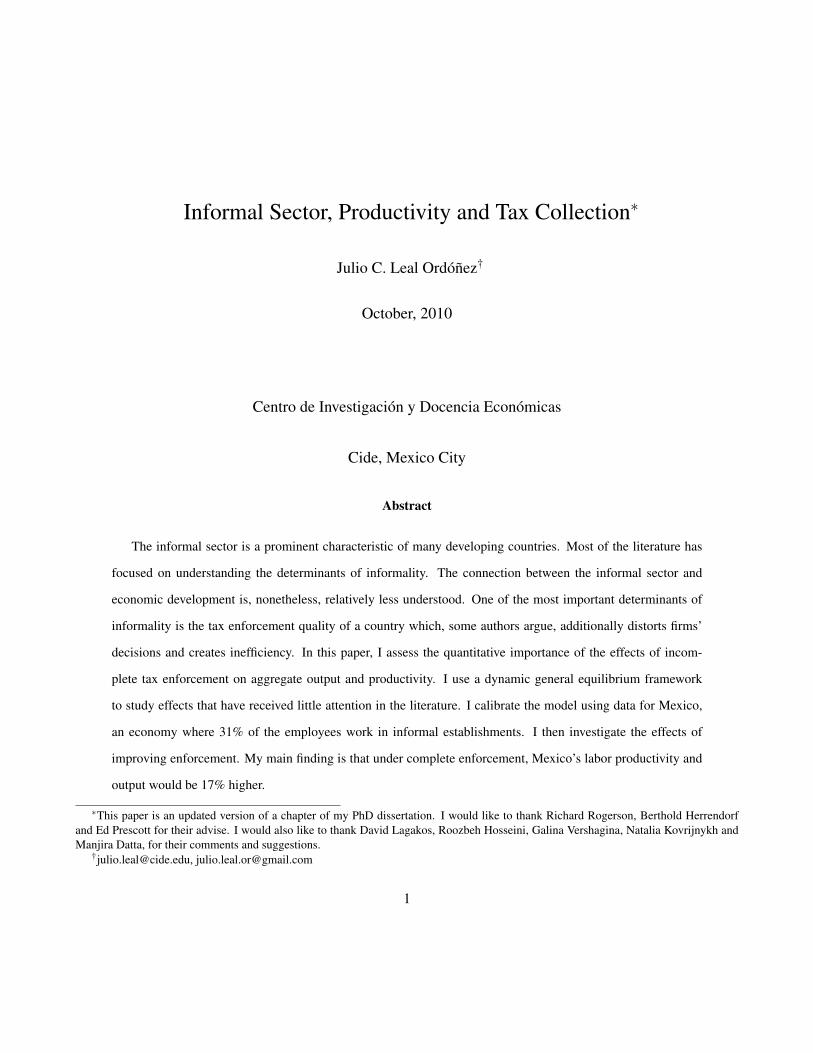
Informal Sector, Productivity and Tax Collection∗

Julio C. Leal Ordóñez†

October, 2010

Centro de Investigación y Docencia Económicas

Cide, Mexico City

Abstract

The informal sector is a prominent characteristic of many developing countries. Most of the literature has

focused on understanding the determinants of informality. The connection between the informal sector and

economic development is, nonetheless, relatively less understood. One of the most important determinants of

informality is the tax enforcement quality of a country which, some authors argue, additionally distorts firms’

decisions and creates inefficiency. In this paper, I assess the quantitative importance of the effects of incom-

plete tax enforcement on aggregate output and productivity. I use a dynamic general equilibrium framework

to study effects that have received little attention in the literature. I calibrate the model using data for Mexico,

an economy where 31% of the employees work in informal establishments. I then investigate the effects of

improving enforcement. My main finding is that under complete enforcement, Mexico’s labor productivity and

output would be 17% higher.

∗This paper is an updated version of a chapter of my PhD dissertation. I would like to thank Richard Rogerson, Berthold Herrendorfand Ed Prescott for their advise. I would also like to thank David Lagakos, Roozbeh Hosseini, Galina Vershagina, Natalia Kovrijnykh andManjira Datta, for their comments and suggestions.

†julio.leal@cide.edu, julio.leal.or@gmail.com

1

1 Introduction

The informal sector is a prominent characteristic of many developing countries. In recent years, there has been a

large body of empirical work that tries to understand what determines the size of the informal.1Nonetheless, we are

still far from understanding the relationship between the informal sector and the stage of economic development

(La Porta and Shleifer (2008)).

Is the informal sector good or bad for development? Some authors have argued that firms operating in the

informal sector are less regulated and less taxed than firms in the formal sector, which allows them to operate more

efficiently. This, represents a positive force for development (see Schneider and Enste (2002)). In contrast, other

authors have highlighted distortions that might arise in the presence of a large informal sector. For example, Lewis

(2004) argues that informality distorts the “natural” competitive process as informal firms enjoy of an “unfair” cost

advantage through tax avoidance; Farrell (2004) reports that some informal firms reduce their scale of operation

in order to remain undetected by the government, which makes them less efficient; and Levy (2008) states that

informality is a drag on the development process because it subsidizes employment in low-productive activities.

In this paper, I study the connection between the informal sector and economic development. I am interested in

quantifying the effects on output and productivity of distortions associated with informality. To do this, I develop

a general equilibrium model of occupational choice and capital accumulation that includes a tax collection policy

with limited enforcement. Individuals have heterogeneous entrepreneurial abilities (as in Lucas (1978)) and each

faces a discrete occupational choice: whether to be a formal entrepreneur, an informal entrepreneur or an employee.

If formal, the entrepreneur pays taxes, if informal, the entrepreneur faces a probability of being caught that depends

positively on the amount of capital hired.

The novelty in this paper is to connect informal sector data for a typical developing country to a general

equilibrium model where the consequences of informality can be studied. I calibrate the model using data for

Mexico, an economy where 31% of the employees work in informal establishments. I then investigate the effects

1Perry et al. (2007) provide a review. See also Loayza (2007) and Schneider (2004).

2

of improving enforcement. My main finding is that under complete enforcement, Mexico’s labor productivity and

output would be 17% higher. To my knowledge, this is the first paper to provide a quantitative assessment of the

effects of incomplete tax enforcement and to articulate the key economic channels through which these effects

occur.

To understand the distortionary aspects of incomplete enforcement it is important to look at two key features of

the equilibrium. The first is that entrepreneurs with low productivity choose informality, while the most productive

ones choose to operate in the formal sector. The reason for this is that any firm below a certain threshold can avoid

detection and so can costlessly operate informally and increase profits by avoiding taxes. Since low productivity

entrepreneurs naturally choose lower scale, tax avoidance acts as an implicit subsidy to establishments with low

productivity. This feature induces two types of distortions: a misallocation of resources to establishments with

low productivity; and a change of entry decisions of entrepreneurs with low ability which increases the number of

unproductive establishments in the economy.

The second feature of the equilibrium is that an important group of informal establishments optimally reduces

its scale to remain undetected by the government. This brings a distortion in the capital-labor ratio of informal

establishments because the probability of being caught is increasing on the amount of capital hired.

When complete enforcement is introduced, these burdens on labor productivity disappear. I find that the re-

moval of these distortions would bring total factor productivity (TFP) and output up by 4% in the short run. Fur-

thermore, I find that, in the long run there would be an increase of 22% in the capital stock and of 11% in output.

There would be also a gain associated with a tax reduction. Under complete enforcement, the tax base is

broadened, so a smaller tax rate would collect the same revenue as before. This is precisely the core of Lewis

(2004) hypothesis who argues that the combination of a big government and incomplete enforcement, leads to the

need of charging high taxes to the most productive part of the economy. I find that Mexico could lower taxes from

a rate of 26% to one of 16% if enforcement was complete. This reduction will increase output further to a level

17% higher than the one in the benchmark economy with informality.

My paper relates to the literature in the following way. First, there are models where the informal sector arises

3

from incomplete enforcement of taxes and/or regulations: Rauch (1991), Amaral and Quintin (2006), Dabla-Norris

et al. (2008) and de Paula and Scheinkman (2007). However, the main focus of these authors is on the determinants

of informality rather than on its consequences. To my knowledge, this is the first paper to provide a quantitative

assessment of the effects of incomplete tax enforcement.

Second, the burdens on productivity associated with informality can be understood as an specific case of the

type of idiosyncratic distortions studied by the literature on resource misallocation across heterogeneous plants and

TFP, identified with the recent work of Restuccia and Rogerson (2008), Guner et al. (2008), and Hsieh and Klenow

(2007). The first two use US as their benchmark and impose hypothetical policies that affect the prices faced by

individual establishments, while the third one studies the cases of China and India. My paper concentrates on the

Mexican case and takes a specific policy that distorts the prices faced by individual producers. In the same line,

there is also the study case of Gollin (1995) for Ghana, where the importance of taxes on large establishments on

productivity is analyzed. One important difference between Gollin (1995) and this paper is that the enforcement

policy considered by Gollin does not distort the capital-labor ratios of informal establishments. As for the case

of Mexico, a related paper is Anton and Hernandez (2010) where they also analyze the informal sector but ask a

different question and use a different methodology.

After this paper was completed, the unpublished work by Moscoso-Boedo and D’Erasmo (2009) was brought

to my attention, which also study the aggregate effects of informality. It is worth noticing that the two papers

emphasize different channels, while I focus on the scale effects of incomplete tax enforcement, they highlight the

importance of debt enforcement as in Amaral and Quintin (2010). There are several other methodological dif-

ferences between the two papers. Perhaps the most important one is that Moscoso-Boedo and D’Erasmo (2009)

assume that formal and informal firms draw from different productivity distributions with the mean of the distribu-

tion of formal firms being larger. In contrast, I assume that both formal and informal entrepreneurs draw from the

same distribution. I make this assumption because it imposes discipline on my exercise and allows me to study the

endogenous implications of informality.

The paper is organized as follow. Section 2 presents data documenting relevant facts about the informal sector

4

and the resource allocation in Mexico; Section 3 presents an overview of the rest of the paper and the main goals;

Section 4 presents the model, while Section 5 characterize the steady state equilibrium; in Section 6, I calibrate the

model, and in 7, I present the results. The last section concludes.

2 Facts

In this section, I use data to document the following facts: 1) the informal sector in Mexico is large, 2) the distri-

bution of labor across establishments sizes in Mexico differs from the one in US, and 3) informal establishments

are small. Additionally, I rely on other studies to document that informal establishments operate with smaller

capital-labor ratios than their formal counterparts.

To address these inquiries, I use a number of household surveys and a census of establishments. I have access

to the microdata of the National Urban Employment Survey (ENEU, by its Spanish acronym), and this is the one I

use more intensively. This survey will not only be helpful to determine the size of the informal sector in terms of

employees, it will also allow me to look at the size of the establishments in it. Additionally, I use other surveys and

a census to complement the information in ENEU and to make comparisons with US data.

2.1 The size of the informal sector

Although the ENEU’s main goal is to measure unemployment, I take advantage of a question addressing whether

the surveyed employee is enrolled at the Mexican Social Security Institute (IMSS) or not. As in many studies on

the informal sector literature, I classify an employee as informal if she/he is not enrolled with IMSS and as formal

otherwise. Using this measure, I obtain that 31% of employees work in the informal sector, as reported in Table

1. The percentage corresponds to ENEU’s survey in the third trimester of 2002. This percentage has not shown

considerable changes during previous years2. Furthermore, Levy (2008) reports a similar figure using a different

methodology that combines establishment data from the Economic Census and IMSS registries.

2Time series are available upon request

5

Table 1: Size of the Informal Sector (ENEU 2002_3)Sector Share

Formal Employees 69.26Informal Employees 30.74

2.1.1 Laws

In this section, I argue that informality is closely associated with lack of enforcement of tax laws. According to

Mexican law, all employers must be registered with IMSS and must register their employees as well. Employers

who do not follow this mandate are able to avoid the payment of IMSS contributions of their employees. The

payment of IMSS contributions entitles the worker with a bundle of benefits including medical coverage in IMSS

hospitals, a savings account for retirement and a savings account for housing.

There are two controversial issues that challenge the suitability of this measure as a proxy for incomplete

enforcement. First, one could make the argument that the actual savings of avoiding IMSS registration are zero

since a worker will only accept a job without IMSS benefits if she/he is compensated with a higher wage. However,

this won’t be the case if IMSS benefits are not valued by workers as much as they cost; and/or if in the absence of

IMSS coverage workers have access to other non-expensive type of health and Social Security services.

Levy (2008), has shown that poor workers in particular (the majority in Mexico), do not value IMSS coverage

fully as explained by the difficulty of access to IMSS hospitals specially borne by these type of workers. Fur-

thermore, since 1997, Mexican Government has provided free alternative Medical coverage to those workers not

enrolled with IMSS (the Seguro Popular). This means that an employee gets a larger wage in the formal sector than

in the informal one, despite the fact that total earnings (which include the value of benefits) are the same in both

sectors. From the point of view of a firm, however, the cost of an informal employee is lower than the cost of a

formal one. For these reasons, the actual savings of a firm avoiding IMSS registration are substantial.

The ENEU survey is not useful to determine if the employer that avoids IMSS registration also avoids other kind

of taxes and regulations. However, with the help of the Micro-business survey, ENAMIN, I conclude below that

this is more likely than not. To make this point, however, I first need to study the characteristics of establishments

6

in the informal sector, which I do later in the next subsection.

2.2 Establishments size distribution

Here, I present data on the size distribution of establishments in Mexico including both the formal and the informal

sectors. I compare this to the distribution in the US, which I take as a relatively undistorted economy. Then, as a

second step, I repeat the comparison using only information on the Mexican formal sector.

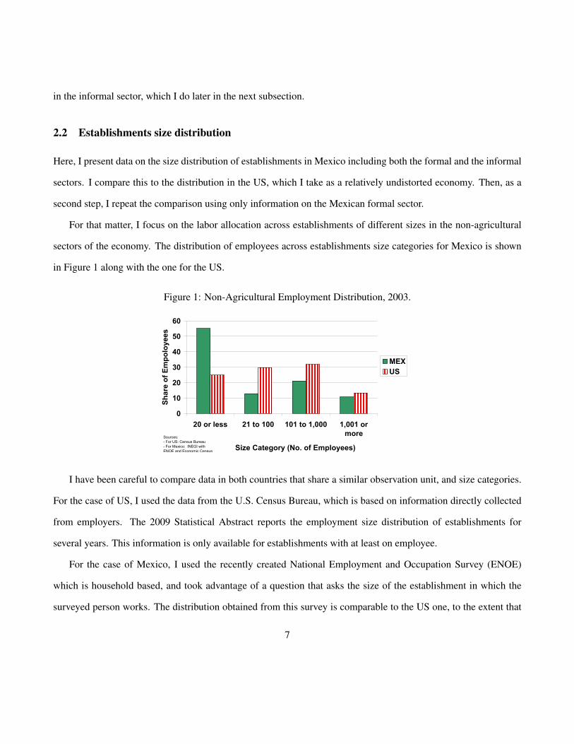
For that matter, I focus on the labor allocation across establishments of different sizes in the non-agricultural

sectors of the economy. The distribution of employees across establishments size categories for Mexico is shown

in Figure 1 along with the one for the US.

Figure 1: Non-Agricultural Employment Distribution, 2003.Mexico vs. US

0

10

20

30

40

50

60

20 or less 21 to 100 101 to 1,000 1,001 or

more

Size Category (No. of Employees)

Share

of Em

polo

yees

MEX

US

Sources:

- For US: Census Bureau

- For Mexico: INEGI with

ENOE and Economic Census

I have been careful to compare data in both countries that share a similar observation unit, and size categories.

For the case of US, I used the data from the U.S. Census Bureau, which is based on information directly collected

from employers. The 2009 Statistical Abstract reports the employment size distribution of establishments for

several years. This information is only available for establishments with at least on employee.

For the case of Mexico, I used the recently created National Employment and Occupation Survey (ENOE)

which is household based, and took advantage of a question that asks the size of the establishment in which the

surveyed person works. The distribution obtained from this survey is comparable to the US one, to the extent that

7

the employees report the size of the establishment with the same accuracy as their employers. This problem is

somewhat mitigated by the use of broadly defined size categories. Alternatively, I could have used the Mexican

Economic Census which is based on information collected from employers. Unfortunately the Census does not

include establishments not using fixed structures, which in the case of Mexico is not negligible. In contrast, the

ENOE, by construction, includes this type of establishment.

One final issue I had to address, was the definition of size categories. The ENOE does not report size categories

comparable to the US in the right tail, and these are of some importance not only for the current comparison, but

especially for later exercises in the paper. Since, virtually all large establishments use fixed structures, I expect the

Census and ENOE not to differ much each other in the right tail. To obtain the full distribution for Mexico then,

I used the Census information to complement the one in ENOE. For more details on how these two sources were

combined see the Appendix3.

In Figure 1, the height of the bar represents the fraction of employees in each size category. It is clear that

the Mexican distribution concentrates more labor in establishments with less than 20 employees. While in Mexico

around 55% of the employees are employed in these small establishments, the figure is only 25% in the US. The

opposite happens for the case of bigger establishments. Hence, when compared to the US, it is clear that Mexico

allocates much more resources in small establishments.

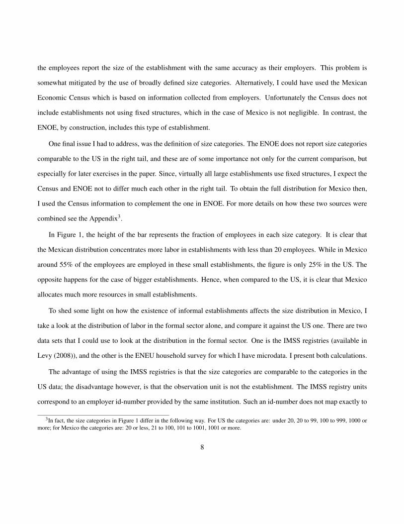
To shed some light on how the existence of informal establishments affects the size distribution in Mexico, I

take a look at the distribution of labor in the formal sector alone, and compare it against the US one. There are two

data sets that I could use to look at the distribution in the formal sector. One is the IMSS registries (available in

Levy (2008)), and the other is the ENEU household survey for which I have microdata. I present both calculations.

The advantage of using the IMSS registries is that the size categories are comparable to the categories in the

US data; the disadvantage however, is that the observation unit is not the establishment. The IMSS registry units

correspond to an employer id-number provided by the same institution. Such an id-number does not map exactly to

3In fact, the size categories in Figure 1 differ in the following way. For US the categories are: under 20, 20 to 99, 100 to 999, 1000 ormore; for Mexico the categories are: 20 or less, 21 to 100, 101 to 1001, 1001 or more.

8

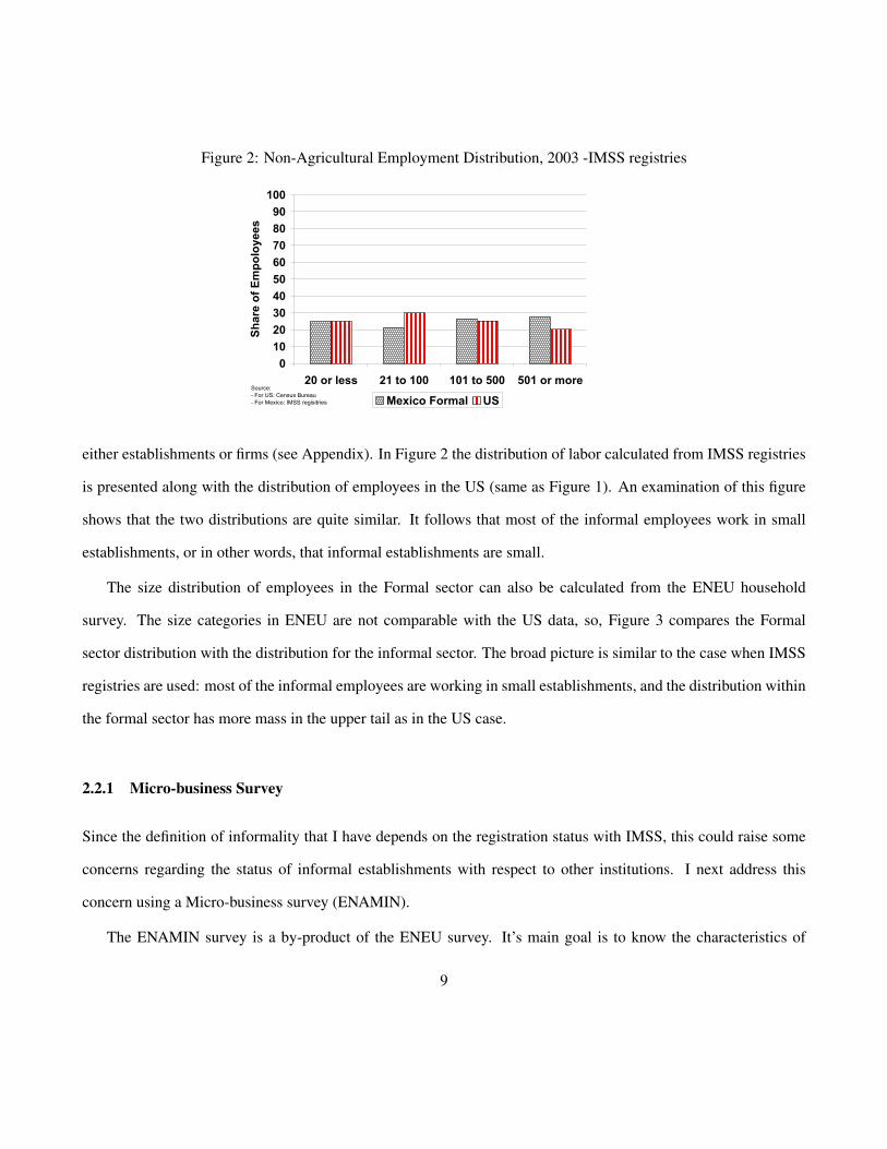
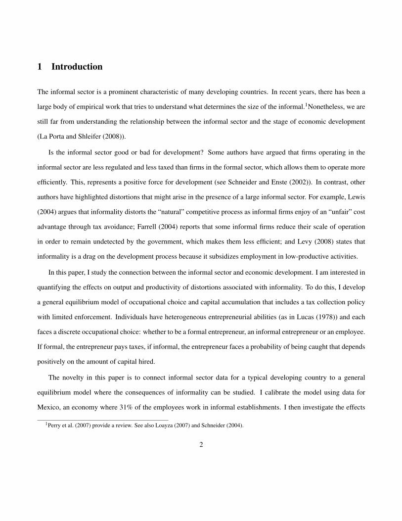
Figure 2: Non-Agricultural Employment Distribution, 2003 -IMSS registriesMexico Formal vs. US

0

10

20

30

40

50

60

70

80

90

100

20 or less 21 to 100 101 to 500 501 or more

Share of Empoloyees

Mexico Formal US

Source:

- For US: Census Bureau

- For Mexico: IMSS regisitries

either establishments or firms (see Appendix). In Figure 2 the distribution of labor calculated from IMSS registries

is presented along with the distribution of employees in the US (same as Figure 1). An examination of this figure

shows that the two distributions are quite similar. It follows that most of the informal employees work in small

establishments, or in other words, that informal establishments are small.

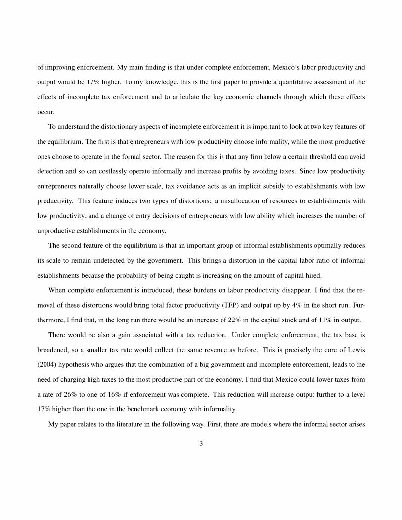
The size distribution of employees in the Formal sector can also be calculated from the ENEU household

survey. The size categories in ENEU are not comparable with the US data, so, Figure 3 compares the Formal

sector distribution with the distribution for the informal sector. The broad picture is similar to the case when IMSS

registries are used: most of the informal employees are working in small establishments, and the distribution within

the formal sector has more mass in the upper tail as in the US case.

2.2.1 Micro-business Survey

Since the definition of informality that I have depends on the registration status with IMSS, this could raise some

concerns regarding the status of informal establishments with respect to other institutions. I next address this

concern using a Micro-business survey (ENAMIN).

The ENAMIN survey is a by-product of the ENEU survey. It’s main goal is to know the characteristics of

9

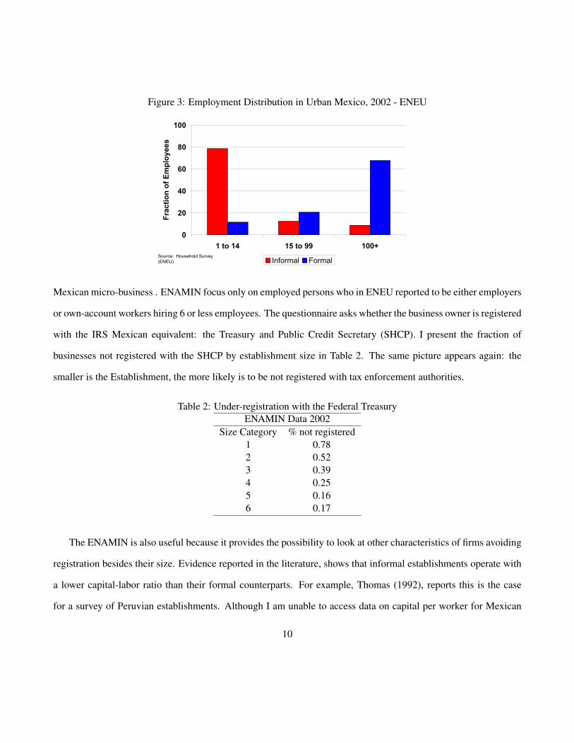
Figure 3: Employment Distribution in Urban Mexico, 2002 - ENEUMexico Formal vs. Mexico Informal

0

20

40

60

80

100

1 to 14 15 to 99 100+

Fraction of Employees

Informal FormalSource: Household Survey

(ENEU)

Mexican micro-business . ENAMIN focus only on employed persons who in ENEU reported to be either employers

or own-account workers hiring 6 or less employees. The questionnaire asks whether the business owner is registered

with the IRS Mexican equivalent: the Treasury and Public Credit Secretary (SHCP). I present the fraction of

businesses not registered with the SHCP by establishment size in Table 2. The same picture appears again: the

smaller is the Establishment, the more likely is to be not registered with tax enforcement authorities.

Table 2: Under-registration with the Federal TreasuryENAMIN Data 2002

Size Category % not registered1 0.782 0.523 0.394 0.255 0.166 0.17

The ENAMIN is also useful because it provides the possibility to look at other characteristics of firms avoiding

registration besides their size. Evidence reported in the literature, shows that informal establishments operate with

a lower capital-labor ratio than their formal counterparts. For example, Thomas (1992), reports this is the case

for a survey of Peruvian establishments. Although I am unable to access data on capital per worker for Mexican

10

informal establishments, for what is worth, I use the ENAMIN to look at the differences in the use of capital

between informal and formal establishments. This information is summarized in Table 3. In particular notice that

81% of businesses in the ENAMIN that report not being registered with SHCP also report the absence of fixed

structures (a physical premise permanently stick to the ground) to perform their productive activities. When only

employers are considered, the percentage is still high (74%).

Table 3: Percentage w/o fixed structures (ENAMIN, 2002)Not Registered Registered

All Businesses 81% 24%Only Employers 74% 14%

3 Overview

The previous section documented three facts. First, 31% of the employees are in the informal sector; two, that

Mexico’s size distribution of employees allocates much more mass to small establishments than the US distribution;

and the third, that most of the informal establishments are small. Additionally, there is evidence in the literature

that informal establishments operate with smaller capital-labor ratios than their formal counterparts.

The goal of this paper is to investigate the extent to which the size distribution of establishments in Mexico

is a result of a distortion induced by incomplete enforcement, and to assess the consequences of this distortion to

the size distribution on labor productivity. In the hypothesis advanced by Lewis (2004), low-productive informal

entrepreneurs take market share from the high-productive formal firms by enjoying the gains of tax avoidance.

Despite their higher productivity, formal firms face a comparative disadvantage to price under informal because

they face the burden of high taxes. In words of La Porta and Shleifer (2008), the informal sector acts as a “parasite”,

surviving at the expense of formal firms.

The Lewis conjecture shares an identical feature with the one studied by the literature on resource misallocation

(e.g Restuccia and Rogerson (2008), Guner et al. (2008) and Hsieh and Klenow (2007)). There, establishments

11

face “idiosyncratic” distortions which affect individual prices, and therefore the allocation of resources and TFP.

In Lewis, incomplete enforcement of tax collection also constitutes the presence of “idiosyncratic distortions”;

informal entrepreneurs face no taxes and formal ones do, therefore, resources are inefficiently allocated towards

the former.

Notice that, this does not mean in any way that the differences between Mexico and US distributions are due

solely to incomplete enforcement differences. For example, it could be argued that Mexico’s skewed distribution

is just a result of its early stage of development. A number of authors have documented the increasing trend of the

average firm size in US during the 19th and 20th century (for a short bibliography, see Desmet and Parente (2009)).

However, when one looks at the distribution in US in the past, at a point in time during which US had the same GDP

per capita than current Mexico (around the 1930’s), it is clear that it wasn’t as concentrated in small establishments

as Mexico is today4. Therefore, it is reasonable to think that the large concentration of labor resources in small

establishments in today’s Mexico is at least in part influenced by incomplete enforcement and the presence of the

informal sector.

With this in mind, I proceed to build a model with heterogeneous entrepreneurial abilities and a tax collection

policy with limited enforcement. This policy, consists on a probability of being caught that depends positively

on the amount of capital hired by the tax avoider. This will lead to an endogenously determined informal sector

where establishments with low productivity sort into informality. This specification captures the fact that smaller

establishments are more likely to be informal and the they show a smaller capital-labor ratio.

4In Granovetter (1984), it is documented that the fraction of employees in US Manufacturing establishments with less than 20 employeesis 10% in 1933 while in 2005 Mexico the fraction of employees in Manufacturing establishments with less than 15 workers is 37.5%. Noticethat the size category is caped at a smaller size for Mexico than for the US, nonetheless the fraction allocated is larger. Similarly, for thesame size categories I find that for the retail and wholesale sectors, the figures are 63.8% and 44.4% in 1939 for the US while it is 72% and48% for Mexico in 2005.

12

4 Economic Environment

The economy is populated by a continuum of individuals of mass 1. At period zero, each individual is endowed

with entrepreneurial ability z ∈ [z,z] and ks0(z) units of capital. This entrepreneurial ability is distributed according

to pdf g(z) and cdf G(z) and it doesn’t evolve over time. Additionally, individuals have 1 unit of time each period

and preferences over a sequence of consumption goods defined by:

∞

∑t=0

βtu(ct(z)) (1)

Where ct(z) is the consumption of individual z in period t. They accumulate capital by making investments

xt(z), and as is standard, the accumulation is determined the following rule:

kst+1(z) = xt(z)+(1−δ )ks

t (z).

Each individual faces a discrete occupational choice, either to become an entrepreneur in the formal sector, an

entrepreneur in the informal sector or an employee in either the formal or the informal sector.

Regardless of the formality status, if an individual with entrepreneurial ability z decides to be a entrepreneur,

she has access to the technology f (z,k, l) = zkθk lθl and 0 < θk +θl < 1, and I define γ = θk +θl . This technology

exhibits decreasing returns to scale ensuring the coexistence of establishments with heterogeneous productivities.

If, on the other hand, the individual decides to be an employee, the indivdual supplies 1 unit of labor which yields

income w, independently of the value of z.

A government levies a tax τy on output, and the revenue is given back to the individuals as a symmetric lump

sum transfer. However, the entrepreneurs can avoid paying taxes by choosing to be in the informal sector. An

output tax is equivalent to levy taxes on labor, capital and entrepreneurial profits (before taxes) simultaneously.

The implicit assumption is that these three margins are taxed at the same rate. Later, I analyze how deviations from

this assumption affect the results of the experiments performed.

13

Tax avoidance comes with a cost. In particular, I assume that informal entrepreneurs face a probability of being

caught, in which case, a punishment is applied. Once caught, the individual will be allowed to have a fresh start

in the next period facing the same occupational choice. The specification of the probability of being caught will

be referred as the enforcement function. I focus on a function that depends on the amount of capital hired in the

establishment. Later in the paper I assume that the probability of being caught could depend alternatively on the

labor hired or the output produced. Perhaps not surprisingly, the results show that when the enforcement policy

depends on capital, the negative effects of incomplete enforcement on accumulation are larger. The following is

assumed:

p(k(z)) =

0, k(z)0 b

1, else, (2)

where k(z) is the capital hired by entrepreneur z and b > 0.

A key feature of the punishment policy is that its level is set high enough to reduce informal profits (if caught)

to a level below formal profits. For simplicity, the punishment is set equal to the current period earnings.

This enforcement policy, gives the opportunity to informal entrepreneurs to choose to operate with a capital

level equal to b or lower, low enough not to get caught by the government while still enjoy the benefits of tax

avoidance.

The step-wise specification might look too restrictive for the reader, so a comment on the advantages and dis-

advantages of this choice is worth remarking at this point. In terms of the equilibrium characterization of the

occupational choices, this specification and any other that includes a strictly increasing probability of being caught

are equivalent. Both will characterize occupational choices with two thresholds in the range of entrepreneurial abil-

ities z (see section 5). The step-wise specification chosen, however, has a clear advantage in terms of computational

burden; it saves the need for solving numerically a nonlinear system of equations for each point of my grid. The

14

specification choice nonetheless will affect the distortion suffered by informal establishments in their capital-labor

ratios; but in the absence of good data on these ratios, I chose the step-wise specification for convenience.

4.1 Individual earnings

Now I analyze the choices of individual agents in more detail. It is optimal for an individual to maximize earnings

in each period by choosing one out of the three possible occupations: employee, informal entrepreneur, formal

entrepreneur. I assume employees are free to move across sectors and therefore they are indifferent between the

two. An individual working as an employee will simply earn wage w.

The earnings in the formal sector for an individual with entrepreneurial ability z are:

πF(z;w,r) = max{lF ,kF}

{(1− τy)zkθk

F lθlF −wlF − rkF

}, (3)

where w is the wage rate and r is the price of capital. I denote by kF(z,w,r) and lF(z,w,r) the optimal choices of

capital and labor respectively in the problem above. Next consider the problem faced by an entrepreneur in the

informal sector. The expected profits of an informal entrepreneur are given by:

πI(z;w,r) = max{lI ,kI}

{(1− p(kI))

(zkθk

I lθlI −wlI− rkI

)}.

I denote by kI(z,w,r) and lI(z,w,r) the optimal choices of capital and labor respectively. Notice that it is not

optimal for any informal entrepreneur to operate with capital larger than b (otherwise her profits will be zero).

However it could choose to operate with capital equal to b, just low enough not to get caught by the government

while still enjoy the benefits of tax avoidance. Therefore the profits of an entrepreneur in the informal sector can

also be expressed as:

15

πI(z;w,r) = max{lI ,kI}

{zkθk

I lθlI −wlI− rkI

}s.t. kI 0 b (4)

Once the profits in the formal and informal sectors are defined for each z, the occupational choice will be taken

to maximize the following earnings function:

e(z;w,r) = (1− I−F)w+ IπI(z;w,r),+FπF(z;w,r),

where I and F equal 1 if the occupation is formal or informal entrepreneur respectively. I use I(z;w,r) and

F(z;w,r) to represent occupational optimal decisions. Similarly, let the index function, Ic(z;w,r) be defined for the

case when an agent decides to be an informal constrained entrepreneur (kI(z,w,r) = b).

4.2 Government

In the present model, the government obtains revenue from two different sources: tax revenue and enforcement

punishments. It turns out that because of the nature of the enforcement policy, revenue from punishments will be

zero in equilibrium. I assume a balanced budget for the government in every period so that all proceeds from gov-

ernment activities are given back to the individuals in the form of a symmetric lump sum transfer. The government

budget balance condition is:

Rt = Tt , ∀t (5)

where Rt is tax revenue.

16

4.3 Consumption decisions of individuals

Once earnings are determined in each period, the individuals take consumption and saving decisions. The occu-

pational, consumption and saving decisions are summarized in the following problem. Taking as given the price

sequences {wt ,rt}, taxes τy and b, an individual with ability z chooses sequences {ct(z),kst (z), It(z),Ft(z)} to solve:

max{ct(z),kt(z),It(z),Ft(z)}

{∞

∑t=0

βtu(ct(z))

}(6)

Subject to the following budget constraint:

ct(z)+ kst+1(z)− (1−δ )ks

t (z) = rtkst (z)+ e(z;wt ,rt ;τy,b)+Tt (7)

where ks0 is given. I focus on the steady state (SS) equilibrium of this economy. As standard, the first order

conditions of this problem in the steady state imply that:

r =1β− (1−δ ) (8)

4.4 Market Clearing

The Market clearing condition for the labor market will equate the aggregate labor demand made by the two sectors

to labor supply:

ˆ z̄

zI(z;wt ,rt)lI(z;wt ,rt)dG(z)+

ˆ z̄

zF(z;wt ,rt)lF(z;wt ,rt)dG(z) =

ˆ z̄

zW (z;wt ,rt)dG(z) (9)

where W (z;wt ,rt) = 1− I(z;wt ,rt)−F(z;wt ,rt). Market clearing for the capital and good markets are respec-

tively:

17

ˆ z̄

zI(z;wt ,rt)kI(z;wt ,rt)dG(z)+

ˆ z̄

zF(z;wt ,rt)kF(z;wt ,rt)dG(z) =

ˆ z̄

zks

t (z)dG(z),

and,

ˆ z̄

zct(z)dG(z)+

ˆ z̄

zks

t+1(z)dG(z)− (1−δ )

ˆ z̄

zks

t (z)dG(z) =

ˆ z̄

zI(z;wt ,rt)yI(z;wt ,rt)dG(z)+

ˆ z̄

zF(z;wt ,rt)yF(z;wt ,rt)dG(z).

4.5 Equilibrium Definition

An equilibrium for this economy is sequences {ct(z),kst+1(z),wt ,rt , It(c),Ft(z)} ∀z ∈ [z,z] , such that taking factor

prices {wt ,rt} and policies parameters τy and b, each individual solves her problem, firms maximize profits ∀t, and

markets clear ∀t.

4.6 Steady State

In what follows I will focus on the steady state equilibrium. Because I define time-invariant tax and enforcement

policies, the dynamic part of this economy is no different than the one in the standard growth model. In the steady

state, factor prices, occupational decisions, aggregate capital and output are constant over time.

5 Model Properties

In this section I analyze some properties of the model. The steady state equilibrium is characterized by three

thresholds {z1,zc,z2} that summarize the occupational decisions of the agents and whether the capital choices of

informal entrepreneurs are constrained or unconstrained. I study the determination of these thresholds next.

Standard arguments on the monotonicity of entrepreneurial profits ensure the existence of a threshold z1 such

18

that w = πM(z1;w,r), where πM(z;w,r) = max{πI(z;w,r),πF(z;w,r)} ,∀z. It follows that all agents with z < z1 will

become employees and the rest entrepreneurs. Also standard are the optimal decisions of formal entrepreneurs:

kF(z,w,r) = ((1− τy)z)1

1−γ

(θl

w

) θl1−γ(

θk

r

) 1−θl1−γ

, (10)

lF(z,w,r) = ((1− τy)z)1

1−γ

(θl

w

) 1−θk1−γ(

θk

r

) θk1−γ

, (11)

and therefore maximum profits can be expressed as a function of prices and parameters:

πF(z,w,r) = (1− γ)((1− τy)z)1

1−γ

(θl

w

) θl1−γ(

θk

r

) θk1−γ

. (12)

A less standard feature of the model is the one related with the presence of the informal sector. As mentioned

before, some entrepreneurs in the informal sector will be better-off by hiring capital equal to b, just low enough

not to be caught. The threshold zc is defined so that all informal entrepreneurs with z < zc operate unconstrained

with kI(z,w,r)< b while all those z≥ zc operate constrained, i.e. kI(z,w,r) = b. To see that this is indeed the case,

consider an entrepreneur z in the informal sector for whom kI(z,w,r) < b. The optimal capital demand for this

entrepreneur will be identical to the one given by equation (10) but replacing τy = 0. As is clear, the monotonicity

of this demand function with respect to z ensures the existence of the threshold zc as defined above. Hence, the

optimal informal profits are expressed in terms of prices and parameters only by:

πI(z;w,r) =

(1− γ)z

11−γ

(θlw

) θl1−γ(

θkr

) θk1−γ

, kI(z,w,r)< b

(1−θl)z1

1−θl

(θlw

) θl1−θl b

θk1−θl − rb, kI(z,w,r) = b

. (13)

How does profits in the informal sector compare to profits in the formal sector for a given entrepreneur z? It

turns out that if b > 0 and τy > 0 is not too large, there exists a threshold z2 such that πI(z2;w,r) = πF(z2;w,r). It

follows that entrepreneurs with ability z < z2 prefer the informal sector and the rest prefer the formal one.

19

To see this, first notice that both the informal and formal entrepreneurs profits are increasing convex functions

of z (because the exponent of the entrepreneurial ability is 11−γ

> 1). Second, notice that by comparing equation

(12) and the top case of equation (13), it is clear that at least for all z 0 zc, informal profits are larger than formal

profits. This is trivially true for other entrepreneurs to the right of zc. Finally, notice that 11−γ

> 11−θl

and hence

as z→ ∞, πF(z;w,r) > πI(z;w,r). This implies the existence of a threshold z2 such that πI(z2;w,r) = πF(z2;w,r)

provided that b > 0 and τy > 0 is not too large.

In order to have a steady state equilibrium where both the informal and formal sectors are positive, it is neces-

sary that b > 0 is not too small and that τy > 0 is not too large. When τy is large, the profits in the formal sector

remain below the profits in the informal sector for all the range of existing entrepreneurial abilities [z, z̄]. If that is

the case, then all entrepreneurs become informal. For example, in the case τy = 1 formal sector’s profits are zero

for all z ∈ [z, z̄], and therefore when b > 0 all entrepreneurs are informal. Similarly, when b = 0, profits in the infor-

mal sector are zero regardless of the ability level, and all entrepreneurs become formal if τy < 1. For intermediate

cases, the size in the informal sector will be positive provided that b > 0 is not too small, otherwise the profits in

the informal sector could remain low for all agents when compared to either, employee earnings or formal profits.

Finally notice that if in equilibrium both the informal and the formal sectors are positive it must be that not all of

the informal entrepreneurs are unconstrained or otherwise the threshold z2 would not exist.

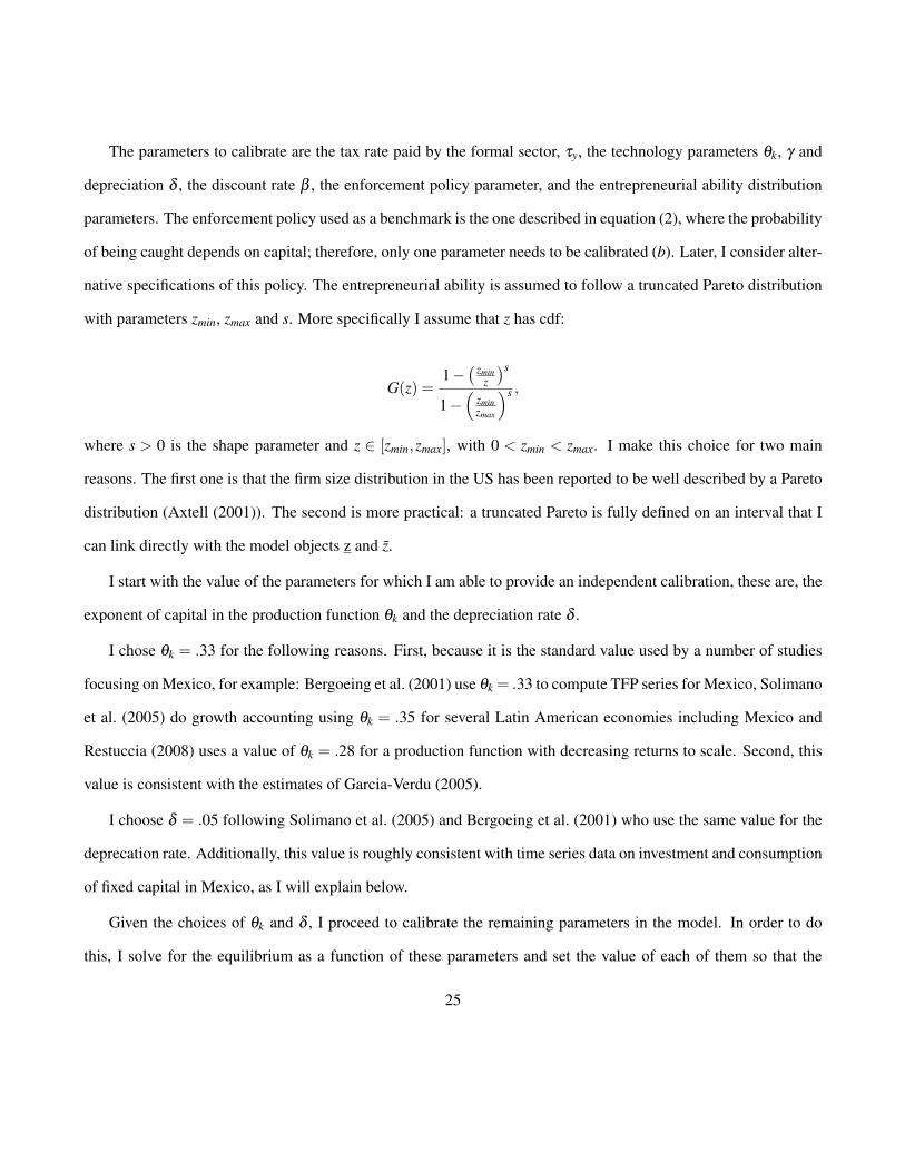
An graphical example of the optimal occupational choices can be found in Figure 4 on page 22, while a full

characterization is given in the following:

Proposition 1. In a steady state equilibrium with positive formal and informal sectors, there exists thresholds

{z1,zc,z2} such that:

1) ∀z ∈ [z,z1) individuals decide to be employees;

2) ∀z ∈ [z1,z2) individuals are informal entrepreneurs;

3) ∀z ∈ [z2, z̄] individuals are formal entrepreneurs;

4) when zc > z1individuals z ∈ (zc,z2) are informal constrained entrepreneurs; and when zc 0 z1 informal

20

entrepreneurs are all constrained.

Proof. The proof was just discussed in the text.

It is convenient to establish some other properties of the equilibrium that will be useful to characterize the

informal sector.

Proposition 2. In an equilibrium with positive informal and formal sectors, the capital demand schedule has a

discontinuity (see Figure 5 on the next page).

Proof. As note above, if both sectors are positive, it must be that the more able informal entrepreneurs are con-

strained. Consider the entrepreneur indifferent between the two sectors z2. If informal, it would hire b capital, if

formal, it would hire an amount strictly larger than b. To see this notice that optimal decisions of entrepreneur z2

are the same optimal decisions of an hypothetical entrepreneur that operates unconstrained and paying no taxes,

this entrepreneur is zh = (1− τy)z2. entrepreneur z2 hires capital strictly larger than b as long as zh > zc, and this

inequality holds because as shown in the bottom case of equation (13), πI(z;w,r) is strictly increasing.

Corollary 3. In an equilibrium with positive informal and formal sectors, the labor demand schedule is strictly

increasing with respect to z

Proof. It follows from the proof of the proposition above.

This discontinuity in the capital schedule translates into an informal sector that looks less capital intensive.

The capital-employee ratio is smaller as well as the capital-output ratio. Next I address some properties of the

equilibrium that will be useful in the calibration and results parts. Consider the following:

Proposition 4. In a steady state equilibrium with positive informal sector, an increase in τy reduces the em-

ployee/entrepreneur threshold z1.

21

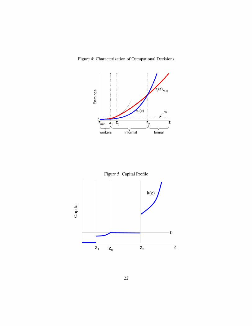
Figure 4: Characterization of Occupational Decisions

workers Informal formal

Figure 5: Capital Profile

Capital

z1 zc z2 z

b

k(z)

22

Proof. Consider first the effects of reducing τy while holding factor prices fixed. Formal profits are reduced for

all entrepreneurial abilities, therefore the threshold z2 increases, switching some entrepreneurs from the formal

to the informal sector. The effect of this, is to reduce aggregate labor demand by two channels: by constraining

new informal entrepreneurs and by the direct effect of larger taxes on previously formal entrepreneurs. Therefore,

aggregate labor demand decreases putting downward pressure on wages. Since the rental rate of capital is constant

across steady states, the wage goes down and the employee/entrepreneur threshold as well.

The decrease in the employee/entrepreneur threshold has important consequences on the employment size

distribution of establishments. I will use this property later in the calibration and results part. The following

moments are affected by the change in τy:

1. The mean size: µ = G(z1)1−G(z1)

,

2. The share of employees in establishments with l̄ or more employees for l̄ > µ . This moment is defined as

follow: sl̄ =´ z̄

x l(z;w,r)dG(z)G(z1)

, where x is the entrepreneur for whom l(x;w,r) = l̄.

3. The mean size of establishments with l̄ or more employees for l̄ > µ . This moment is defined as follow:

µl̄ =´ z̄

x l(z;w,r)dG(z)1−G(x)

Corollary 5. In a steady state equilibrium with a positive informal sector, an increase in τy reduces moments 1,2

and 3.

Proof. Number 1 follows from the definition of mean size: µ = G(z1)1−G(z1)

. Number 2 follows from 1 because less

density is necessary above the original mean if I are going to reduce it. The last point is more subtle. Define x as

the entrepreneur for whom l(x;w,r) = l̄, notice that this moment is defined as:

µl̄ =

´ z̄x l(z;w,r)dG(z)

1−G(x)=

´ z̄x l(z;w,r)dG(z)

G(z1)

1−G(x)G(z1)

.

23

Clearly, the numerator is smaller because of 2 and the denominator is larger because both G(z1) and G(x) fall.

The drop in G(z1) is a restatement of Proposition 4 and the drop in G(x) happens because as mentioned in the proof

of proposition 4, each entrepreneur demands less employees after the tax is reduced.

Finally, I stress one important role played by the span of control parameter γ as summarized by the following:

Proposition 6. In an equilibrium with a positive informal sector, an increase in either θk or θl , increases the

employee/entrepreneur threshold z1.

Proof. This follows from the Cobb-Douglas assumption of the production function. The effect of increasing γ is to

reduce the fraction of value added by the entrepreneurs, and therefore her earnings. Marginal entrepreneur z1 won’t

be indifferent anymore and will become a employee. This is trivially true for entrepreneurs to the right of z1.

Corollary 7. In an equilibrium with a positive informal sector, an increase in either θk or θl increases moments 1,

2 and 3.

Proof. For moments 1 and 2 the proof is the same as the one for Corollary 5. For moment number 3, the proof is

almost identical except that now the reason G(x) increases is associated with the fact that labor demand is larger

for every entrepreneur as a result of the change in its marginal productivity.

6 Calibration

In this section I describe the calibration strategy. Since I target a developing country (Mexico), there is a distinc-

tion with the strategies followed by works that focus on developed economies such as the ones in Restuccia and

Rogerson (2008) and Guner et al. (2008). There, it is assumed that US has small distortions and the distortion

free scenario is used as a benchmark to study how deviations affect equilibrium variables. In the case of this paper

however, the distorted nature of the Mexican Economy prevents us from following the same approach.

24

The parameters to calibrate are the tax rate paid by the formal sector, τy, the technology parameters θk, γ and

depreciation δ , the discount rate β , the enforcement policy parameter, and the entrepreneurial ability distribution

parameters. The enforcement policy used as a benchmark is the one described in equation (2), where the probability

of being caught depends on capital; therefore, only one parameter needs to be calibrated (b). Later, I consider alter-

native specifications of this policy. The entrepreneurial ability is assumed to follow a truncated Pareto distribution

with parameters zmin, zmax and s. More specifically I assume that z has cdf:

G(z) =1−( zmin

z

)s

1−(

zminzmax

)s ,

where s > 0 is the shape parameter and z ∈ [zmin,zmax], with 0 < zmin < zmax. I make this choice for two main

reasons. The first one is that the firm size distribution in the US has been reported to be well described by a Pareto

distribution (Axtell (2001)). The second is more practical: a truncated Pareto is fully defined on an interval that I

can link directly with the model objects z and z̄.

I start with the value of the parameters for which I am able to provide an independent calibration, these are, the

exponent of capital in the production function θk and the depreciation rate δ .

I chose θk = .33 for the following reasons. First, because it is the standard value used by a number of studies

focusing on Mexico, for example: Bergoeing et al. (2001) use θk = .33 to compute TFP series for Mexico, Solimano

et al. (2005) do growth accounting using θk = .35 for several Latin American economies including Mexico and

Restuccia (2008) uses a value of θk = .28 for a production function with decreasing returns to scale. Second, this

value is consistent with the estimates of Garcia-Verdu (2005).

I choose δ = .05 following Solimano et al. (2005) and Bergoeing et al. (2001) who use the same value for the

deprecation rate. Additionally, this value is roughly consistent with time series data on investment and consumption

of fixed capital in Mexico, as I will explain below.

Given the choices of θk and δ , I proceed to calibrate the remaining parameters in the model. In order to do

this, I solve for the equilibrium as a function of these parameters and set the value of each of them so that the

25

model replicates a number of features of the Mexican economy. These features are the ratio of total tax revenue

to GDP, various moments of the size distribution of employment, the size of the informal sector and the aggregate

capital-output ratio.

The data for the moments of the size distribution of employment and the size of the informal sector was

described in Section 2. The data for the other two targets (the capital-output ratio and the revenue to GDP ratio)

has not being decribed before.

An assesment of the magnitude of the capital-output ratio is needed. For this matter, I use data on the consump-

tion of fixed capital (as a fraction of GNI) from Indicators (2005), and take the average since 1980 (which I call d).

This average is around 10%. The model counterpart of d is δK/Y . Since δand d are known, I solve for K/Y from

this equation and obtain K/Y = d/δ = .10/.05 = 2.

This value of the capital-output ratio is close to the one found in two independent studies that estimate the

capital stock in Mexico. Hofman (2000) performs a disaggregated estimation by type. The implied capital-output

ratio in his work is around 1.7. Restuccia (2008) uses data from the Penn World Tables to estimate the capital-output

ratios of a number of Latin American countries. He finds a value for Mexico of around 1.9.

As a check, I used the capital accumulation equation in the balanced growth path combined with data on invest-

ment and capital consumption to jointly calculate the capital-output ratio and the depreciation rate. Specifically,

I take yearly data on the Gross fixed capital formation (%GDP) and the consumption of fixed capital (%GNI)

from Indicators (2005), and take averages since 1980; then I solved the following system of equations: (1):

(1+ n)(1+ g)(K/Y ) = (1− δ )(K/Y )+ (I/Y ), and (2) δ (K/Y ) = d. Where n and g are the annual population

and technology growth rates respectively, and d = 0.105. I set n = .02 and g = .025, again using data since 1980.

The two unknowns are (K/Y ) and δ . I get K/Y = 1.9 and δ = .059.

The ratio of government tax revenue as a fraction of GDP is calculated in the following way. According to

OECD.stat, total tax revenue in 2003 was $1,312,246.9183 million pesos and according to INEGI the GDP in 2003

was 6,891,992.482 million pesos. This gives a ratio of 19% of GDP.

One important outcome of the calibration is the value of the implicit tax rate paid by the formal sector and

26

avoided in the informal. Ideally I would like to have a measure of the savings that an informal entrepreneur is able

to achieve. For this matter, I would have to not only make a full characterization of the Mexican tax code, but also

to consider non tax savings or expenditures such as bribes and red tape. Furthermore, for some taxes such as the

Social Security contributions it is important to consider the worker’s benefits valuation because these are key in

determining the actual savings of hiring informal workers.

Instead of attempting to figure out each of the components of the implicit taxes, I have assumed that the informal

savings can be summarized by an output tax that captures all the costs of operating formal. I will assume first that

all of these costs come exclusively from the tax burden and that there are no costs of regulation. Notice in particular

that the value of τy should be larger if there are non-tax costs associated with formality such as labor, sanitary and

environmental regulations. Put differently, recent news blame informal firms of “stealing” electricity, so another

cost associated with formality is the full payment of electric bills. On the other hand, there could be non-tax costs

associated with informality such as bribes that will tend to reduce the value of τy. Because of these issues, I also

report results for the case where positive non-tax costs of formality are considered.

I also perform a sensitivity analysis to investigate how the model’s outcomes change when alternative tax types

are in place. There are three type of idiosyncratic distortions that a firm can experience in the model: on labor

prices, capital prices and on the value added by the entrepreneur5. A tax on total output will be equivalent to a tax

on all three margins simultaneously. To assess the importance of each of them I consider independently the cases

of taxes on output, labor, capital and entrepreneurial output.

Also worth noticing is that the discount rate β can not be calibrated in the usual way. The usual way consists on

obtaining a value of r from the FOC of the firms and then using this value in the Euler equation to determine β . In

principle, one could think that the FOC of the formal establishments can be used to find the value of r; but for that I

would need an estimation of the capital-output ratio in the formal sector, which is not available. Mexico’s National

Accounts include an estimation of the informal sector, and since I used National Accounts data to estimate the K/Y

5In this model there are only three factors: capital, labor and entrepreneurs. However, in practical terms, the value not added by capitaland labor can not entirely be attributed as value added from entrepreneurial services, since it also corresponds to the contribution of otherfactors not considered here such as “organizational capital”.

27

ratio, I think of it as a ratio that includes the capital and the output from both sectors.

6.1 Matching Moments

The remaining parameters are τy, γ, zmin, zmax, s, b and β . The choice of zmin is, to some extent, arbitrary. This is

due to the fact that all individuals with entrepreneurial ability below the z1 threshold become identical employees

(their ability is transformed into 1 unit of labor). Therefore, what matters in equilibrium is the mass of individuals

to the left of z1. Once zmin is set, this mass is fully determined by the parameters that describe the distribution of

entrepreneurial abilities.

The rest of the parameter values are obtained by matching moments of the plant size distribution, the capital-

output ratio, tax revenue and the size of the informal sector measured as a fraction of employees. In the model there

is a weakly monotonic equilibrium relationship between the size of a productive unit in terms of the labor employed

and its entrepreneurial ability (see corollary 3). I take advantage of this feature to calibrate the parameters of the

entrepreneurial ability distribution. I use the employment distribution of establishments across size categories as

well as information on the average size of the units in each category for this regard6. The moments targeted are:

1. the average size of establishments in the economy,

2. the average size of establishments with more than 100 workers,

3. the fraction of workers in establishments with more than 100 workers,

4. the size of the informal sector, and

5. the capital-output ratio.

6. Tax revenue as a fraction of GDP

It is worth noticing that by targeting the first three moments, I will also match their complements: the share of

workers and the average size of establishments with 100 workers or less. How well will I match similar moments for6This procedure is close to those in Guner et al. (2008) and Rubini (2009)

28

more disaggregated size categories will depend only on the structure imposed by the Pareto distribution. As I show

below, the calibration yields estimated parameters that replicate the data fairly well even at a high disaggregated

level of size categories, despite the fact that I do not target such moments. I present a summary of the calibration

targets in Table 4.

Table 4: Calibration Targets SummaryParameter Target Source

θk capital share Gollin (2002);Garcia-Verdu (2005)

δ gross capital formation; WDI,consumption of fixed capital; Solimano et al. (2005) and

Bergoeing et al. (2001)zmin arbitrary -

γ

β moments of distribution; Matchingzmax size of informal sector; moments

s capital-output ratioτy Tax revenue/GDPb

As part of the sensitivity analysis, I performed calibration exercises for a number of cases varying both the type

and levels of taxes and the type of enforcement policy considered. Each exercise needed an independent calibration,

hence, different calibrated parameters emerged in each case.

6.2 Calibration Properties

The targeted moments are well matched as can be confirmed in Table 5, where I present data and model values.

Perhaps more interesting, is the fact that the calibration yields parameters that replicate well a number of mo-

ments that were not targeted explicitly. In Table 6, it is shown that the model replicates the mean size and the labor

shares for a number of highly disaggregated size categories. This is an important check for the methodology used,

because by replicating the allocation of labor across categories that differ in average size, I am in fact replicating

labor allocation across productivity levels.

29

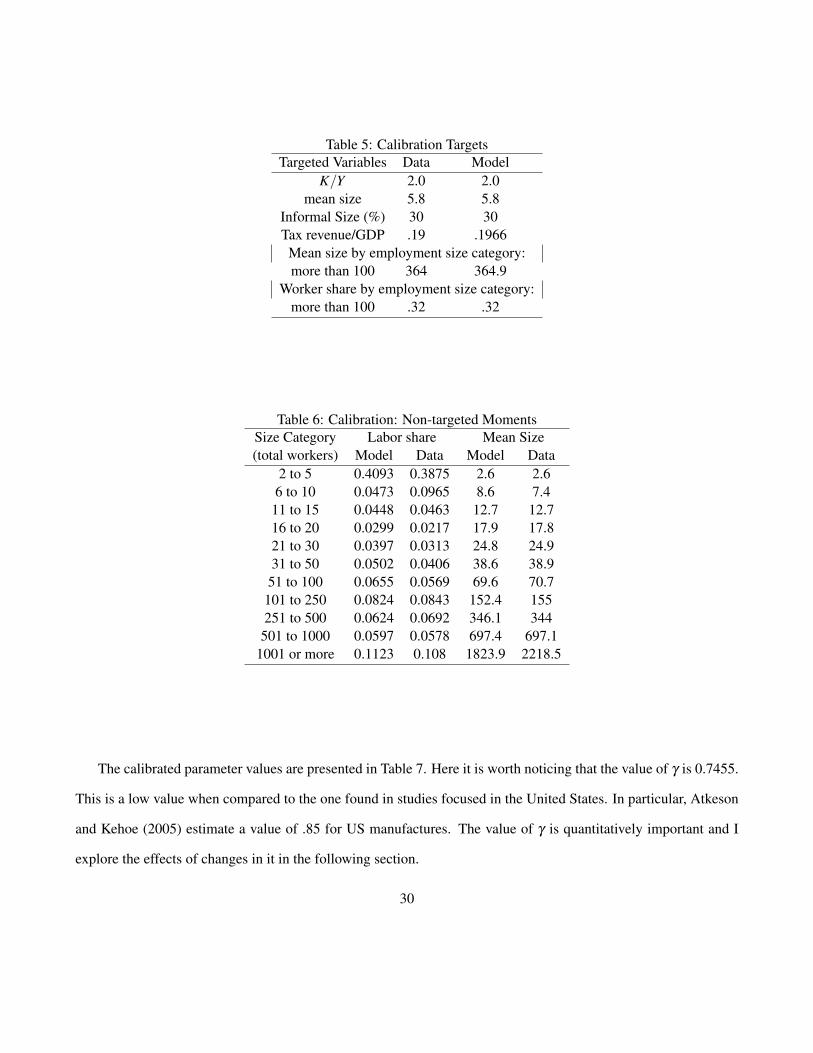
Table 5: Calibration TargetsTargeted Variables Data Model

K/Y 2.0 2.0mean size 5.8 5.8

Informal Size (%) 30 30Tax revenue/GDP .19 .1966

Mean size by employment size category:more than 100 364 364.9

Worker share by employment size category:more than 100 .32 .32

Table 6: Calibration: Non-targeted MomentsSize Category Labor share Mean Size(total workers) Model Data Model Data

2 to 5 0.4093 0.3875 2.6 2.66 to 10 0.0473 0.0965 8.6 7.411 to 15 0.0448 0.0463 12.7 12.716 to 20 0.0299 0.0217 17.9 17.821 to 30 0.0397 0.0313 24.8 24.931 to 50 0.0502 0.0406 38.6 38.951 to 100 0.0655 0.0569 69.6 70.7

101 to 250 0.0824 0.0843 152.4 155251 to 500 0.0624 0.0692 346.1 344501 to 1000 0.0597 0.0578 697.4 697.1

1001 or more 0.1123 0.108 1823.9 2218.5

The calibrated parameter values are presented in Table 7. Here it is worth noticing that the value of γ is 0.7455.

This is a low value when compared to the one found in studies focused in the United States. In particular, Atkeson

and Kehoe (2005) estimate a value of .85 for US manufactures. The value of γ is quantitatively important and I

explore the effects of changes in it in the following section.

30

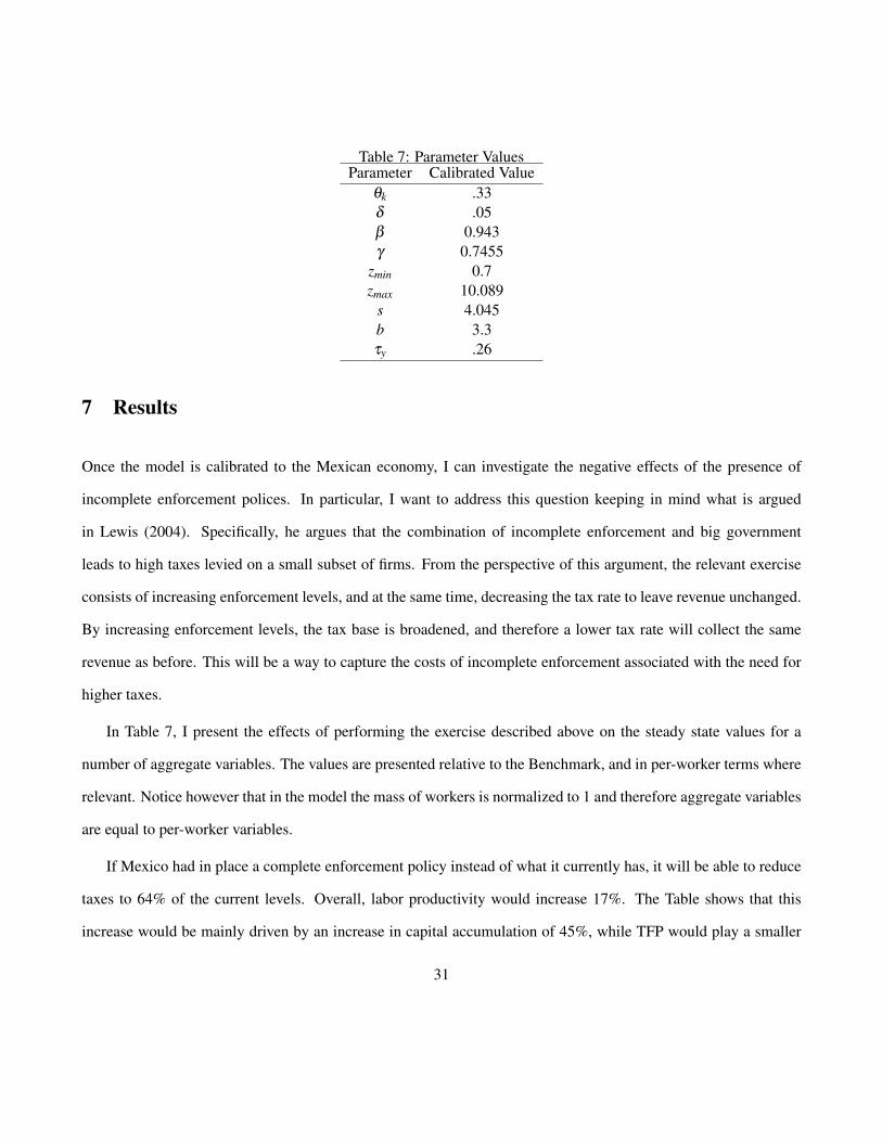
Table 7: Parameter ValuesParameter Calibrated Value

θk .33δ .05β 0.943γ 0.7455

zmin 0.7zmax 10.089

s 4.045b 3.3τy .26

7 Results

Once the model is calibrated to the Mexican economy, I can investigate the negative effects of the presence of

incomplete enforcement polices. In particular, I want to address this question keeping in mind what is argued

in Lewis (2004). Specifically, he argues that the combination of incomplete enforcement and big government

leads to high taxes levied on a small subset of firms. From the perspective of this argument, the relevant exercise

consists of increasing enforcement levels, and at the same time, decreasing the tax rate to leave revenue unchanged.

By increasing enforcement levels, the tax base is broadened, and therefore a lower tax rate will collect the same

revenue as before. This will be a way to capture the costs of incomplete enforcement associated with the need for

higher taxes.

In Table 7, I present the effects of performing the exercise described above on the steady state values for a

number of aggregate variables. The values are presented relative to the Benchmark, and in per-worker terms where

relevant. Notice however that in the model the mass of workers is normalized to 1 and therefore aggregate variables

are equal to per-worker variables.

If Mexico had in place a complete enforcement policy instead of what it currently has, it will be able to reduce

taxes to 64% of the current levels. Overall, labor productivity would increase 17%. The Table shows that this

increase would be mainly driven by an increase in capital accumulation of 45%, while TFP would play a smaller

31

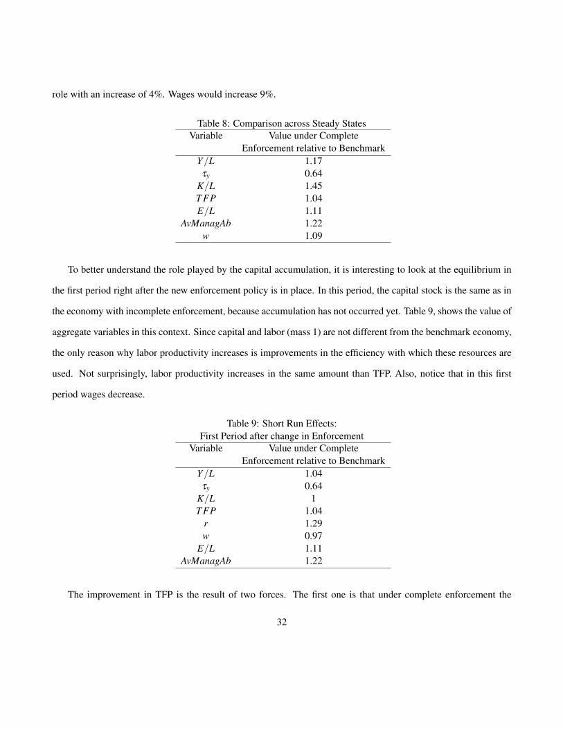
role with an increase of 4%. Wages would increase 9%.

Table 8: Comparison across Steady StatesVariable Value under Complete

Enforcement relative to BenchmarkY/L 1.17τy 0.64

K/L 1.45T FP 1.04E/L 1.11

AvManagAb 1.22w 1.09

To better understand the role played by the capital accumulation, it is interesting to look at the equilibrium in

the first period right after the new enforcement policy is in place. In this period, the capital stock is the same as in

the economy with incomplete enforcement, because accumulation has not occurred yet. Table 9, shows the value of

aggregate variables in this context. Since capital and labor (mass 1) are not different from the benchmark economy,

the only reason why labor productivity increases is improvements in the efficiency with which these resources are

used. Not surprisingly, labor productivity increases in the same amount than TFP. Also, notice that in this first

period wages decrease.

Table 9: Short Run Effects:First Period after change in Enforcement

Variable Value under CompleteEnforcement relative to Benchmark

Y/L 1.04τy 0.64

K/L 1T FP 1.04

r 1.29w 0.97

E/L 1.11AvManagAb 1.22

The improvement in TFP is the result of two forces. The first one is that under complete enforcement the

32

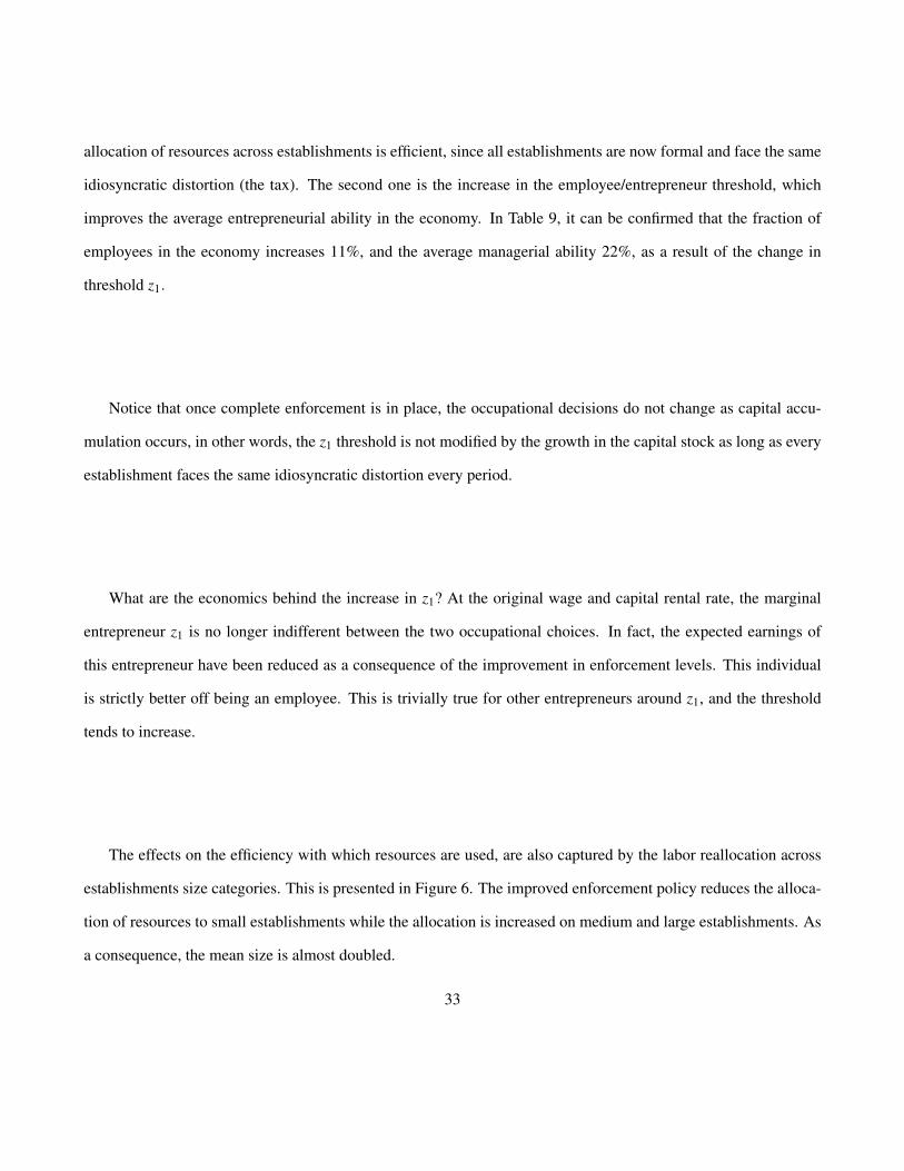
allocation of resources across establishments is efficient, since all establishments are now formal and face the same

idiosyncratic distortion (the tax). The second one is the increase in the employee/entrepreneur threshold, which

improves the average entrepreneurial ability in the economy. In Table 9, it can be confirmed that the fraction of

employees in the economy increases 11%, and the average managerial ability 22%, as a result of the change in

threshold z1.

Notice that once complete enforcement is in place, the occupational decisions do not change as capital accu-

mulation occurs, in other words, the z1 threshold is not modified by the growth in the capital stock as long as every

establishment faces the same idiosyncratic distortion every period.

What are the economics behind the increase in z1? At the original wage and capital rental rate, the marginal

entrepreneur z1 is no longer indifferent between the two occupational choices. In fact, the expected earnings of

this entrepreneur have been reduced as a consequence of the improvement in enforcement levels. This individual

is strictly better off being an employee. This is trivially true for other entrepreneurs around z1, and the threshold

tends to increase.

The effects on the efficiency with which resources are used, are also captured by the labor reallocation across

establishments size categories. This is presented in Figure 6. The improved enforcement policy reduces the alloca-

tion of resources to small establishments while the allocation is increased on medium and large establishments. As

a consequence, the mean size is almost doubled.

33

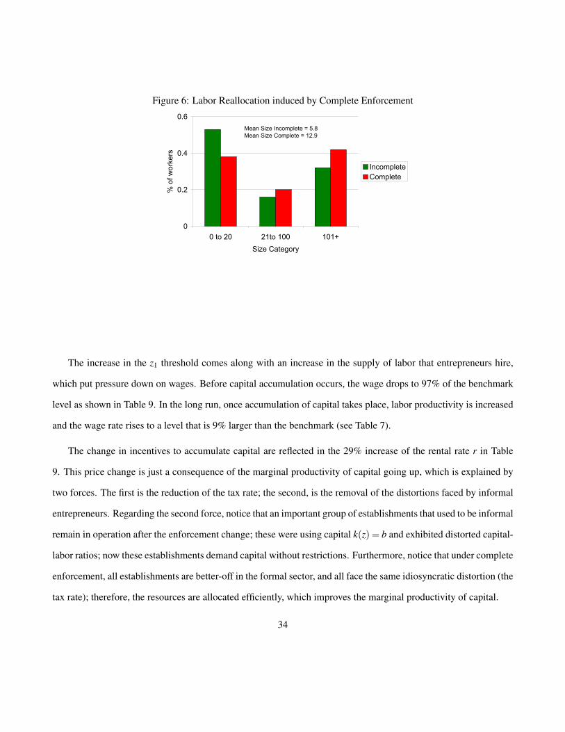
Figure 6: Labor Reallocation induced by Complete EnforcementLabor Reallocation due to Improved Enforcement

0

0.2

0.4

0.6

0 to 20 21to 100 101+

Size Category

% of workers

Incomplete

Complete

Mean Size Incomplete = 5.8

Mean Size Complete = 12.9

The increase in the z1 threshold comes along with an increase in the supply of labor that entrepreneurs hire,

which put pressure down on wages. Before capital accumulation occurs, the wage drops to 97% of the benchmark

level as shown in Table 9. In the long run, once accumulation of capital takes place, labor productivity is increased

and the wage rate rises to a level that is 9% larger than the benchmark (see Table 7).

The change in incentives to accumulate capital are reflected in the 29% increase of the rental rate r in Table

9. This price change is just a consequence of the marginal productivity of capital going up, which is explained by

two forces. The first is the reduction of the tax rate; the second, is the removal of the distortions faced by informal

entrepreneurs. Regarding the second force, notice that an important group of establishments that used to be informal

remain in operation after the enforcement change; these were using capital k(z) = b and exhibited distorted capital-

labor ratios; now these establishments demand capital without restrictions. Furthermore, notice that under complete

enforcement, all establishments are better-off in the formal sector, and all face the same idiosyncratic distortion (the

tax rate); therefore, the resources are allocated efficiently, which improves the marginal productivity of capital.

34

7.0.1 TFP effects

The increase in TFP looks small (4%) from the perspective of explaining the development problem. For example,

Restuccia (2008) reports that in a model with human capital, one would need that US TFP be at least 60% larger

than in Latin America to account for differences in output per worker of a factor of 4.

The main driver of the small gain obtained, is the calibrated value of γ = .75. This value is small when

compared to what has been found in studies focusing in the US (e.g. Atkeson and Kehoe (2005), Guner et al.

(2008)). γ controls the returns to scale at the establishment level. The closer is γ to 1 the lower is the degree

of decreasing returns and the more efficient is to concentrate production in large establishments. In the limiting

case of γ = 1 (constant returns to scale) the efficient output is reached by concentrating all resources in a single

unit: the most productive one. The low value of γ I find, implies that the efficient allocation for Mexico is to

have more workers in small units than countries where the degree of decreasing returns is smaller (i.e., larger γ),

equivalently, it implies that the economy with incomplete enforcement is not too far from the efficient allocation.

In fact, according to this estimate, the efficient allocation for Mexico is to have around 35% of the employees hired

by small establishments (those who hire 20 worker or less). Compare this to a 25% allocation in the US in the same

size category. This is consistent with the results in Figure 6, where it is shown that the reallocation of resources is

small when enforcement is perfect.

An interesting question is: How the results change if γ is set to a value similar to what has been found in

the US (around .85)? It turns out that the structure imposed by the assumption of the underlying entrepreneurial

ability distribution (i.e., that it follows a truncated Pareto distribution) makes impossible to match all the moments

requested before only by varying the parameters of the distribution. In particular, what I find is that I will need to

vary the tax rate along with the distribution parameters to match the desired moments if I keep the returns to scale

parameter fixed. I find that the larger I fix the value of γ , the larger the tax rate needed to match the moments in

section 6.1. Conversely, if I repeat the calibrated exercise and ask to match exactly the same moments as before but

instead of using a tax rate of 26% I use a larger tax rate, the calibrated value of γ needed will be higher.

35

This conjecture can be explained by the use of propositions 4 and 6. Consider the calibrated economy in section

6, this is an economy with incomplete enforcement and an output tax of 26%. What would happen if tax rate is

increased? By proposition 4 I know that the worker/entrepreneur threshold z1 will fall, and by corollary 5 I know

that the moments I targeted are going to be reduced. If the goal is to match the targets back but holding the new tax

rate, it is clear by proposition 6 and corollary 7 that decreasing γ will only take us further away from this goal. It

is intuitive, lower values of γ will only make more low productive entrepreneurs willing to enter, and hence further

reduce the mean average, the fraction of workers in large establishments and its mean size.

I exploit this positive relationship in γ and τy to set an upper bound for the tax rate.

7.0.2 Sensitivity to the tax rate

In Table 7.0.2, I present the results of improving the enforcement policy when the starting tax rate is 50% instead

of 26%. As noted in the Calibration part, the actual savings of being informal could be underestimated by the 26%

used so far. Some costs of being formal are not collected as revenue, such as periodic costs associated with sanitary,

environmental, labor regulations, and the like. To that, one could add bribes and red tape costs as well as entry

costs which are specially high in Latin American countries7.

As expected, the value of γ needed to match the moments of section 6.1 is larger in this case and closer to the

value found by studies focusing on the US case (γ = .83).

Table 10: Steady State Comparisons (τy = .50)Variable Value under Complete

Enforcement relative to BenchmarkY/L 1.53τy 0.53

K/L 2.6T FP 1.12E/L 1.17

AvManagAb 1.26w 1.64

7de Soto (1989), Djankov et al. (2002)

36

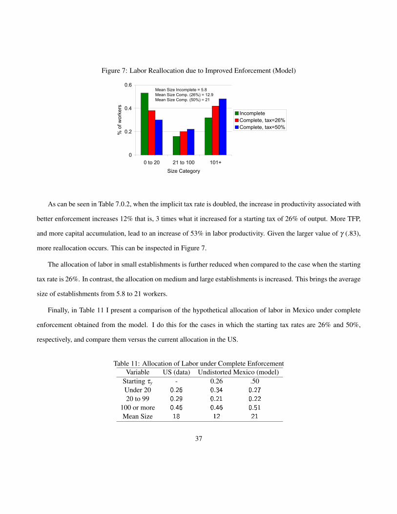
Figure 7: Labor Reallocation due to Improved Enforcement (Model)Labor Reallocation due to Improved Enforcement

(Model)

0

0.2

0.4

0.6

0 to 20 21 to 100 101+

Size Category

% of workers

Incomplete

Complete, tax=26%

Complete, tax=50%

Mean Size Incomplete = 5.8

Mean Size Comp. (26%) = 12.9

Mean Size Comp. (50%) = 21

As can be seen in Table 7.0.2, when the implicit tax rate is doubled, the increase in productivity associated with

better enforcement increases 12% that is, 3 times what it increased for a starting tax of 26% of output. More TFP,

and more capital accumulation, lead to an increase of 53% in labor productivity. Given the larger value of γ (.83),

more reallocation occurs. This can be inspected in Figure 7.

The allocation of labor in small establishments is further reduced when compared to the case when the starting

tax rate is 26%. In contrast, the allocation on medium and large establishments is increased. This brings the average

size of establishments from 5.8 to 21 workers.

Finally, in Table 11 I present a comparison of the hypothetical allocation of labor in Mexico under complete

enforcement obtained from the model. I do this for the cases in which the starting tax rates are 26% and 50%,

respectively, and compare them versus the current allocation in the US.

Table 11: Allocation of Labor under Complete EnforcementVariable US (data) Undistorted Mexico (model)

Starting τy - 0.26 .50Under 20 0.26 0.34 0.27

20 to 99 0.29 0.21 0.22

100 or more 0.46 0.46 0.51

Mean Size 18 12 21

37

The fraction of employees working in firms with 20 or less workers is now 27% which is closer to the 26%

found in the US data. Similarly the average establishment size is increased to 21 workers, which is closer to the

average size in the US.

Notice that if this sensitivity analysis is repeated for a larger value of the tax rate (say 60%), even more real-

location would occur when imposing the complete enforcement policy. Therefore, I conclude with the following

conjecture:τy = .50 is an upper bound for the actual tax rate. This is because a larger tax rate would imply an

efficient allocation in Mexico that would display implausibly large establishments. It would also need of a larger

value of γ than the one found in studies focusing on the US case.

8 Conclusion

The main goal of this paper was to investigate how the presence of informal establishments due to incomplete

enforcement affects the aggregate outcomes in developing countries. Although a long tradition (starting with Harris

and Todaro (1970)) understands the informal sector simply as a symptom of early stages of development; a more

modern literature associated with Lewis (2004), challenges this view. The Lewis hypothesis highlights the harmful

effects of tax collection policies with limited enforcement.

I study a general equilibrium framework that includes a tax collection policy with limited enforcement. I

calibrate the steady state equilibrium of this model to the case of Mexico. I then investigate the effects of improving

enforcement. I find that under complete enforcement, Mexico’s labor productivity would be 17% higher in the new

steady state.

The first lesson learned in the paper is that informality is associated with resource misallocation. This is driven

by the government inability to enforce tax and regulation policies on all firms. As a result, the tax base is small,

and high taxes have to be levied on a small subset of firms, usually the most productive ones. This has a negative

effect on aggregate productivity by misplacing resources into less productive establishments.

A second lesson is that incomplete enforcement not only gives existing establishments with low productivity

38

a cost advantage; it also makes it more attractive for entrepreneurs with low ability to start new businesses. This

distorts the mix of productivities of operating establishments, and therefore productivity.

A third important, perhaps unexpected, lesson is that the nature of enforcement policies reduces output through

its effect on firms’ optimal decisions. In the paper, the specification of the enforcement policy depends on the use

of capital in the establishments. So a group of firms are better off by reducing their capital demands to a level low

enough not to be detected by government authorities. This distorts the capital per worker of informal establishments

and therefore aggregate capital and output.

This paper therefore, emphasizes the gains associated with improving enforcement levels and reducing the

informal sector. I find important gains in productivity and output for countries that at this moment, have a large

fraction of the economic activity under informality.

References

AMARAL, P. AND E. QUINTIN (2010): “Limited Enforcement, Financial Intermediation, And Economic Devel-

opment: A Quantitative Assessment,” International Economic Review, 51, 785–811.

AMARAL, P. S. AND E. QUINTIN (2006): “A Competitive Model Of The Informal Sector,” Journal of Monetary

Economics, 53, 1541–1553.

ANTON, A. AND F. HERNANDEZ (2010): “VAT Collection and Social Security Contributions under Tax Evasion:

Is There a Link?” .

ATKESON, A. AND P. J. KEHOE (2005): “Modeling and Measuring Organization Capital,” Journal of Political

Economy, 113, 1026–1053.

AXTELL, R. (2001): “Zipf distribution of US firm sizes,” Science, 293, 1818–1820.

39

BERGOEING, R., P. KEHOE, T. KEHOE, AND R. SOTO (2001): “A decade lost and found: Mexico and Chile in

the 1980s,” NBER Working Paper.

DABLA-NORRIS, E., M. GRADSTEIN, AND G. INCHAUSTE (2008): “What causes firms to hide output? The

determinants of informality,” Journal of Development Economics, 85, 1–27.

DE PAULA, A. AND J. SCHEINKMAN (2007): “The Informal Sector, Third Version,” PIER Working Paper Archive.

DE SOTO, H. (1989): The Other Path: The Invisible Revolution in the Third World, I B Tauris & Co Ltd.

DESMET, K. AND S. PARENTE (2009): “The Evolution of Markets and the Revolution of Industry: A Quantitative

Model of England’s Development, 1300-2000,” CEPR Discussion Papers 7290, C.E.P.R. Discussion Papers.

DJANKOV, S., R. LA PORTA, F. LOPEZ-DE SILANES, AND A. SHLEIFER (2002): “The Regulation of Entry*,”

Quarterly Journal of Economics, 117, 1–37.

FARRELL, D. (2004): “The hidden dangers of the informal economy,” McKinsey Quarterly, 26–37.

GARCIA-VERDU, R. (2005): “Factor Shares From Household Survey Data,” Working Papers 2005-05, Banco de

MÃ c©xico.

GOLLIN, D. (1995): “Do Taxes on Large Firms Impede Growth? Evidence from Ghana,” Bulletins 7488, Univer-

sity of Minnesota, Economic Development Center.

——— (2002): “Getting Income Shares Right,” Journal of Political Economy, 110, 458–474.

GRANOVETTER, M. (1984): “Small is bountiful: labor markets and establishment size,” American Sociological

Review, 49, 323–334.

GUNER, N., G. VENTURA, AND Y. XU (2008): “Macroeconomic implications of size-dependent policies,” Review

of Economic Dynamics, 11, 721 – 744.

40

HARRIS, J. R. AND M. P. TODARO (1970): “Migration, Unemployment and Development: A Two-Sector Analy-

sis,” The American Economic Review, 60, 126–142.

HOFMAN, A. (2000): “Standardised capital stock estimates in Latin America: a 1950-94 update,” Cambridge

Journal of Economics, 24, 45–86.

HSIEH, C.-T. AND P. J. KLENOW (2007): “Misallocation and Manufacturing TFP in China and India,” Working

Paper 13290, National Bureau of Economic Research.

INDICATORS, W. D. (2005): “World Development Indicators 2005 CD-ROM,” .

LA PORTA, R. AND A. SHLEIFER (2008): “The Unofficial Economy and Economic Development,” SSRN eLi-

brary.

LEVY, S. (2008): Good Intentions, Bad Outcomes: Social Policy, Informality, and Economic Growth in Mexico,

Brookings Institution Press.

LEWIS, W. W. (2004): The Power of Productivity: Wealth, Poverty, and the Threat to Global Stability, University

Of Chicago Press.

LOAYZA, N. (2007): “The causes and consequences of informality in Peru,” Tech. rep., Working Paper Series.

LUCAS, R. E. (1978): “On the Size Distribution of Business Firms,” The Bell Journal of Economics, 9, 508–523.

MOSCOSO-BOEDO, H. J. AND P. N. D’ERASMO (2009): “Financial Structure, Informality and Development,”

Virginia Economics Online Papers 374, University of Virginia, Department of Economics.

PERRY, G., W. MALONEY, O. ARIAS, P. FAJNZYLBER, AND A. MASON (2007): Informality: exit and exclusion,

World Bank Publications.

RAUCH, J. (1991): “Modelling the informal sector formally,” Journal of Development Economics, 35, 33–47.

41

RESTUCCIA, D. (2008): “The Latin American Development Problem,” Working Papers tecipa-318, University of

Toronto, Department of Economics.

RESTUCCIA, D. AND R. ROGERSON (2008): “Policy distortions and aggregate productivity with heterogeneous

establishments,” Review of Economic Dynamics, 11, 707 – 720.

RUBINI, L. (2009): “Innovation and the Elasticity of Trade Volumes to Tariff Reductions,” unpublished.

SCHNEIDER, F. (2004): “The Size of the Shadow Economies of 145 Countries all over the World: First Results

over the Period 1999 to 2003,” IZA DP, 1431.

SCHNEIDER, F. AND D. ENSTE (2002): The shadow economy, Springer.

SOLIMANO, A., R. SOTO, AND U. NATIONS (2005): Economic growth in Latin America in the late 20th century:

evidence and interpretation, United Nations Pubns.

THOMAS, J. J. (1992): Informal Economic Activity, Harvester Wheatsheaf, New York, N.Y.

Appendix

9 Employment Distribution across Establishment size categories

I have been careful to compare figures that share a similar observation unit in both countries. For Mexico I combine

data from the most recent National Employment and Occupations Survey (ENOE) and the Economic Census both

collected by the National Institute of Statistics (INEGI). The observation unit for both is the establishment 8. I am

8Given the peculiarities of the economic activities in Mexico, the observation unit in the census varies with industry codes. For manu-facturing, services and trade the unit of observation was the establishment. These three sectors include 97% of the surveyed units. Data formost of the remaining sectors is collected using the firm as unit of observation. An hybrid unit of observation had to be used for specificindustries such as mining and fishing.

42

in the need to combine these two sources because the Economic Census doesn’t collect information of businesses

that don’t use a building or some kind of physical premise permanently “stick to the ground” and as I have shown,

this are not negligible in the Mexican case. I also want to have a distribution of establishments with employees

only, because that is the way data in US is collected. This means that I need disaggregated data for the lower tier

of the distribution which is only publicly available from ENOE.

Because of the way the Census is performed I believe is a good approximation of the size distribution of

medium and large establishments; using the Micro-business survey ENAMIN, I can establish that the larger the

establishment, the larger the probability of being included in the Census. On the other hand, the ENOE is the best

approximation of the size distribution of small establishments. Therefore, I combine the ENOE and the Census

to obtain a full distribution of employment across size categories. Specifically, I use ENOE data to pin down the

fraction of workers in two size categories: 2 to 5 workers, and 6 or more.

Once I have these numbers, I proceed to break down the distribution for the category of 6 or more. I do

this using the census data. I obtain the distribution of workers across size categories in the census conditional on

having 6 or more workers. It is important to remark that neither the Census nor the ENAMIN are able to describe

fully the distribution of workers across size categories because the ENAMIN is based on owner information (not

establishments) and the Census does not include establishments with out fixed structures as explained.

10 Sensitivity to Enforcement Specification and Tax types

10.1 Considering alternative enforcement policies for the output tax case

In this section I explore the robustness of the results to alternative enforcement policies. I keep the same step-wise

enforcement policy but make the probability of being caught depend on labor and output, each case is considered

independently. The results can be found in Table 12

The effect on output is reduced to 10% when output is used as a signal to enforce tax policy and to 8% when

labor is used. This compares to an increase of 16% when the enforcement depends on capital. The effect on

43

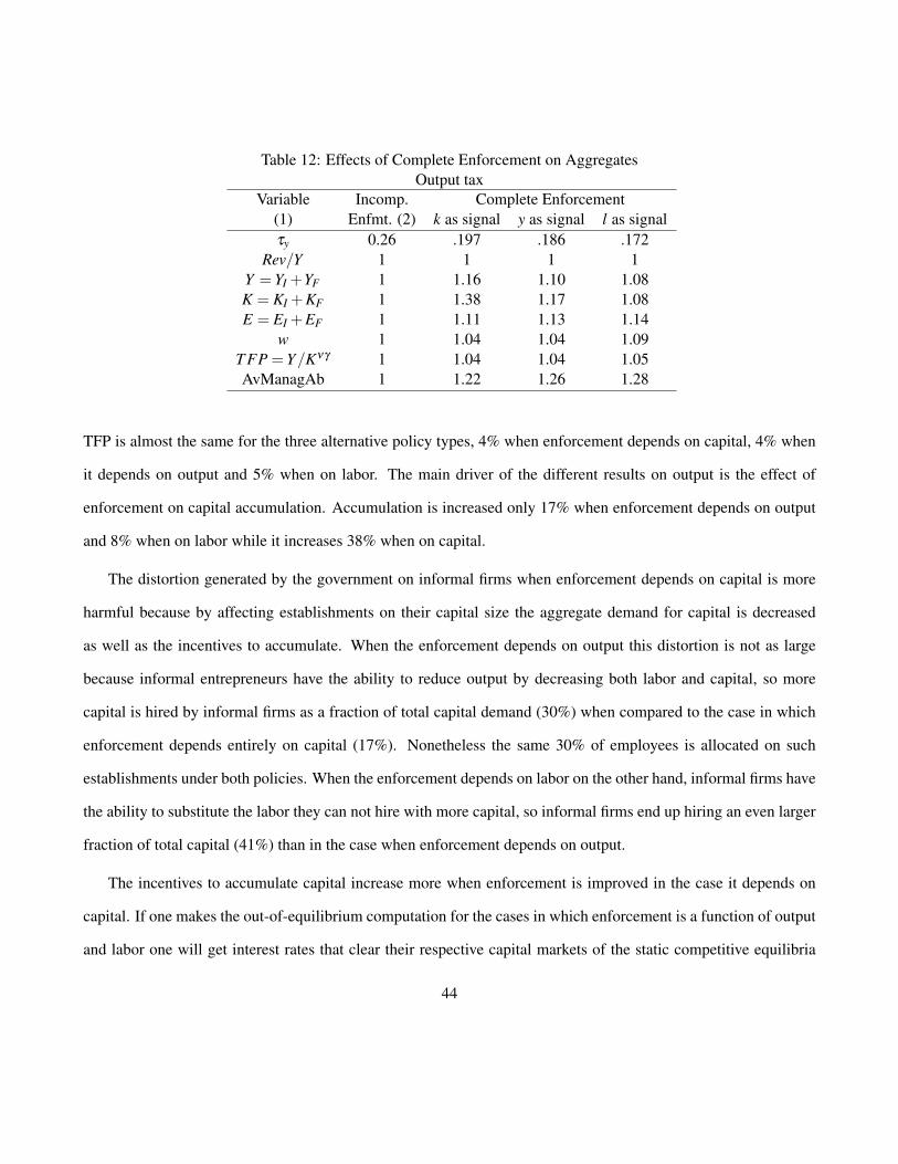
Table 12: Effects of Complete Enforcement on AggregatesOutput tax

Variable Incomp. Complete Enforcement(1) Enfmt. (2) k as signal y as signal l as signalτy 0.26 .197 .186 .172

Rev/Y 1 1 1 1Y = YI +YF 1 1.16 1.10 1.08K = KI +KF 1 1.38 1.17 1.08E = EI +EF 1 1.11 1.13 1.14

w 1 1.04 1.04 1.09T FP = Y/Kνγ 1 1.04 1.04 1.05AvManagAb 1 1.22 1.26 1.28

TFP is almost the same for the three alternative policy types, 4% when enforcement depends on capital, 4% when

it depends on output and 5% when on labor. The main driver of the different results on output is the effect of

enforcement on capital accumulation. Accumulation is increased only 17% when enforcement depends on output

and 8% when on labor while it increases 38% when on capital.

The distortion generated by the government on informal firms when enforcement depends on capital is more

harmful because by affecting establishments on their capital size the aggregate demand for capital is decreased

as well as the incentives to accumulate. When the enforcement depends on output this distortion is not as large

because informal entrepreneurs have the ability to reduce output by decreasing both labor and capital, so more

capital is hired by informal firms as a fraction of total capital demand (30%) when compared to the case in which

enforcement depends entirely on capital (17%). Nonetheless the same 30% of employees is allocated on such

establishments under both policies. When the enforcement depends on labor on the other hand, informal firms have

the ability to substitute the labor they can not hire with more capital, so informal firms end up hiring an even larger

fraction of total capital (41%) than in the case when enforcement depends on output.

The incentives to accumulate capital increase more when enforcement is improved in the case it depends on

capital. If one makes the out-of-equilibrium computation for the cases in which enforcement is a function of output

and labor one will get interest rates that clear their respective capital markets of the static competitive equilibria

44

that are 10% and 5% larger than their corresponding benchmark levels.

10.2 Considering alternative tax types

In this section I explore how the results are affected when I deviate from the assumption that all factors of production

are taxed at the same rate. As formerly noted, a tax on output is equivalent to tax labor, capital and entrepreneurial

output simultaneously at the same rate9 and this could not be the actual case for the Mexican economy. Therefore

in this section I investigate how the effects of improving enforcement levels could change if I modify the distortions

faced by entrepreneurs. I focus on the case of an enforcement policy that depends on capital.

I proceed by taking deviations from the case where all tax rates are 26% (or equivalently the case of an output

tax equal to 26%). I increase one of the taxes at a time and reduce the other two so that the revenue as a fraction of

output remains at 26%. Every time I increase one of the taxes I reduce the other two while keeping them equal to

each other. For example, consider the case in which the capital is taxed more heavily than the other two margins.

A tax on capital of τr = .35 will need tax rates on labor (τw) and entrepreneurial output (τm) of .2336 to keep the

revenue as a share of formal output at .26. Given the choice of these taxes I run the SMM to match the same targets

as before.

Departing from the economy just described I analyze the effects of complete enforcement by comparing it

against an economy with complete enforcement but faces only an output tax set at a level that collects the same

revenue share of the economy with incomplete enforcement. The results for the case in which I increase the tax

rate of capital are presented in Table 10.2.

The accumulation effects of better enforcement are increased when the starting situation taxes capital more

heavily while the effects on TFP remain almost the same. Aggregate output is increased 19% and 23% for the

cases in which the incomplete enforcement case taxes capital at 35% and 45% respectively. The main driver of the

increase in output is the distance between the tax rates payed in the formal sector across enforcement scenarios.

9Specifically, consider the profits of a entrepreneur facing taxes τw, τr and τm on labor, capital and entrepreneurial output respectively.Profits are: π(z, l,k) = zkθk lθl −wl− rk− τwwl− τrrk− τm(zkθk lθl −wl− rk). When τw = τr = τm = τy, then the profits are the same asthose for a entrepreneur facing only tax τy on output.

45

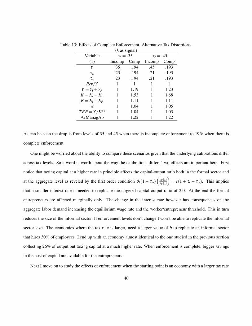
Table 13: Effects of Complete Enforcement. Alternative Tax Distortions.(k as signal)

Variable τr = .35 τr = .45(1) Incomp Comp Incomp Compτr .35 .194 .45 .193τw .23 .194 .21 .193τm .23 .194 .21 .193

Rev/Y 1 1 1 1Y = YI +YF 1 1.19 1 1.23K = KI +KF 1 1.53 1 1.68E = EI +EF 1 1.11 1 1.11

w 1 1.04 1 1.05T FP = Y/Kνγ 1 1.04 1 1.03AvManagAb 1 1.22 1 1.22

As can be seen the drop is from levels of 35 and 45 when there is incomplete enforcement to 19% when there is

complete enforcement.

One might be worried about the ability to compare these scenarios given that the underlying calibrations differ

across tax levels. So a word is worth about the way the calibrations differ. Two effects are important here. First

notice that taxing capital at a higher rate in principle affects the capital-output ratio both in the formal sector and

at the aggregate level as reveled by the first order condition θk(1− τm)(

yF (z)kF (z)

)= r(1+ τr − τm). This implies

that a smaller interest rate is needed to replicate the targeted capital-output ratio of 2.0. At the end the formal

entrepreneurs are affected marginally only. The change in the interest rate however has consequences on the

aggregate labor demand increasing the equilibrium wage rate and the worker/entrepreneur threshold. This in turn

reduces the size of the informal sector. If enforcement levels don’t change I won’t be able to replicate the informal

sector size. The economies where the tax rate is larger, need a larger value of b to replicate an informal sector

that hires 30% of employees. I end up with an economy almost identical to the one studied in the previous section

collecting 26% of output but taxing capital at a much higher rate. When enforcement is complete, bigger savings

in the cost of capital are available for the entrepreneurs.

Next I move on to study the effects of enforcement when the starting point is an economy with a larger tax rate

46

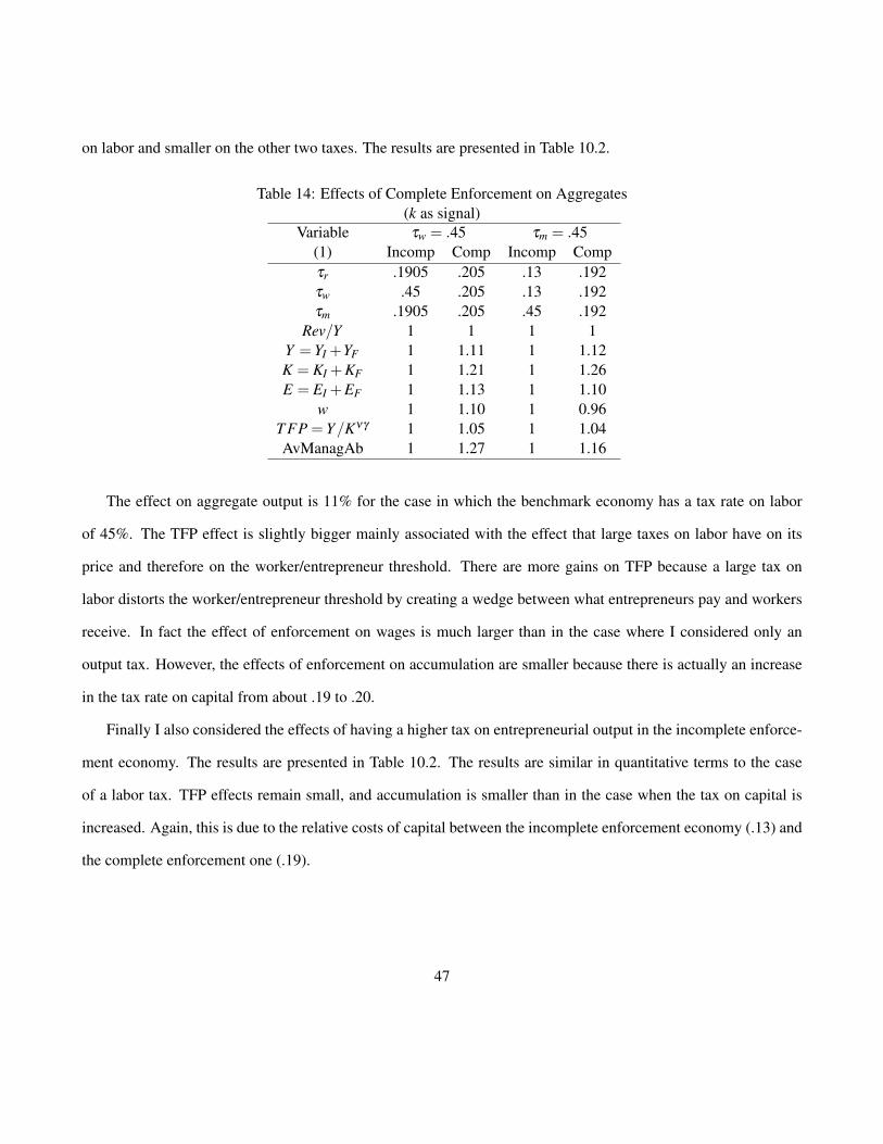
on labor and smaller on the other two taxes. The results are presented in Table 10.2.

Table 14: Effects of Complete Enforcement on Aggregates(k as signal)

Variable τw = .45 τm = .45(1) Incomp Comp Incomp Compτr .1905 .205 .13 .192τw .45 .205 .13 .192τm .1905 .205 .45 .192

Rev/Y 1 1 1 1Y = YI +YF 1 1.11 1 1.12K = KI +KF 1 1.21 1 1.26E = EI +EF 1 1.13 1 1.10

w 1 1.10 1 0.96T FP = Y/Kνγ 1 1.05 1 1.04AvManagAb 1 1.27 1 1.16

The effect on aggregate output is 11% for the case in which the benchmark economy has a tax rate on labor

of 45%. The TFP effect is slightly bigger mainly associated with the effect that large taxes on labor have on its

price and therefore on the worker/entrepreneur threshold. There are more gains on TFP because a large tax on

labor distorts the worker/entrepreneur threshold by creating a wedge between what entrepreneurs pay and workers

receive. In fact the effect of enforcement on wages is much larger than in the case where I considered only an

output tax. However, the effects of enforcement on accumulation are smaller because there is actually an increase

in the tax rate on capital from about .19 to .20.

Finally I also considered the effects of having a higher tax on entrepreneurial output in the incomplete enforce-

ment economy. The results are presented in Table 10.2. The results are similar in quantitative terms to the case

of a labor tax. TFP effects remain small, and accumulation is smaller than in the case when the tax on capital is

increased. Again, this is due to the relative costs of capital between the incomplete enforcement economy (.13) and

the complete enforcement one (.19).

47