Influence of rotor currents on end-winding forces incage motor

S. Williamson, PhD, CEng, FIEEM.R.E. Ellis, MSc, AMIEE

Indexing terms: Induction motors, Electromagnetic theory

Abstract: The paper proposes a simple model thatenables the influence of rotor currents to beincluded in the calculation of the electromagneticforces acting on the end windings of cage induc-tion motors, using the Biot-Savart method. Theinclusion of the rotor currents is shown to havegreatest influence close to core, where the end-region fields are also highest. The validity of themodel is established using experimental measure-ments of flux density made on a two polemachine. Calculated force distributions show theeffect of the rotor currents to be significantenough to merit their inclusion in the model.

1 Introduction

The problem of providing adequate bracing for statorand rotor end-windings, to protect them against the elec-tromagnetic forces that arise during both normal andabnormal operating conditions, has been studied for anumber of years, and has resulted in an extensive liter-ature. The majority of the attention has been focused onturbogenerators, with relatively few authors consideringthe forces acting on the end windings of cage inductionmotors [1-3]. Recent operational experience, particularlyon offshore oil production platforms in the North Sea,has indicated a need for the bracing of induction motorend windings to be reappraised, following serious failureof a large number of high voltage machines. This paperreports the findings of a study that was carried out aspart of that reappraisal. The work described relates spe-cifically to the calculation of electromagnetic forcesacting on the end-windings. The results of a complemen-tary study, concerned with the calculation of deflectionsand natural frequencies, are reported elsewhere [4].

2 Analytical model

2.1 Choice of modelThe techniques that have been used to study the forceson induction motor end-windings derive from thosedeveloped for turbogenerators, and it is appropriatetherefore to review those methods.

Paper 6253B (PI), first received 3rd February and in revised form 18thMay 1988Dr. Williamson is with the Department of Electrical Engineering,Imperial College, London SW7 2BT, United KingdomM.R.E Ellis is with the Central Engineering Department, Shell UKExploration and Production, Shell-Mex House, London WC2R ODX,United Kingdom

Two different calculation techniques appear to havebeen widely adopted. The first, described by Lawrensonin a seminal paper [5], is based on the use of the Biot-Savart law. Each coil in the end-winding is replaced byan equivalent filamentary conductor, carrying the sameampere-turns, and the method of images is used toremove the stator and rotor core ends. The result is a setof filamentary coils, in air, and the forces on the endwindings are calculated from the interactions of these fil-amentary coils. The method has the advantage that it canreadily accommodate any shape of end-coil, any connec-tion of stator coils, and any current loading condition.Furthermore, the method is conceptually simple and rela-tively straightforward to use. On the other hand, Law-renson's method cannot account for the presence offerromagnetic materials in the end region, such as aventilation fan or rotor support ring, nor does it accu-rately represent the other boundaries to the end region.

The second widely used technique is based on the useof the finite element method, which is inherently capableof giving an accurate 3-dimensional solution for the fieldaround the end-region, from which the forces acting canbe calculated. Furthermore, the surfaces bounding theend region may be accurately modelled, as may the fan orany other metallic object present. Unfortunately,although such a 3-dimensional model is now technicallyfeasible, the computer resources required would be soprodigious that workers in this field have been obliged touse a 2-dimensional approximation [6-9]. The under-lying assumption made is that all field quantities vary ina sinusoidal manner in the peripheral direction, and thatthe current-carrying windings may be replaced by anequivalent current sheet. The field solution is then carriedout in the rz plane. The major advantage of this 2-dimensional model is that it gives a realistic representa-tion of cylindrical surfaces around the end region, so thatthe rotor shaft and fan can be included in the model. Themain errors stem from the assumptions made to renderthe problem 2-dimensional.

The forces acting on the end-winding of any machinedepend on the currents flowing in the windings, and aregreatest when the currents are greatest. For an inductionmotor, the maximum force condition will occur duringstarting, particularly if a direct-on-line starter is used.Although it may be argued that the run up period ismore important than starting as far as fatigue life estima-tion is concerned [10] the calculation of maximum forcesis clearly of importance, so that the method used mustreadily be capable of representing an arbitrary set ofinstantaneous currents. Sinusoidal field variation in theperipheral direction implies an ideal stator winding,carrying balanced three-phase currents, although tran-sient or unbalanced currents and nonideal windings

IEE PROCEEDINGS, Vol. 135, Pt. B, No. 6, NOVEMBER 1988 371

might be simulated using a superposition of harmonicsolutions. Lawrensons's method, on the other hand, canaccommodate a general set of stator currents with ease,and for this reason Lawrenson's method was chosen forinvestigation.

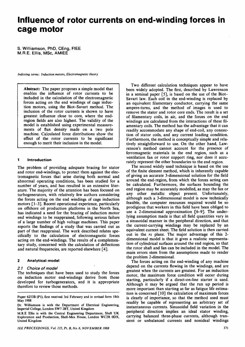
2.2 Representation of rotor currentsThe filamentary model for a single stator end-coil isshown in Fig. 1 [11, 12]. The real (i.e. physically real)

end-windingfilament

the rotor end ring which spans the same arc as thatstator coil. KJIH is therefore an effective stationary

airgapconductor

Fig. 1 Lawrenson's model for stator coil-end

end-coil is represented by the filament CDEFG, C and Gbeing the points at which the coil emerges from the statorstack. Under the assumption that the core end behaveslike an infinitely permeable plane, the image of the realcoil end is shown as CD'E'F'G. The remainder of themodel takes care of the mmf drops across the stator slots(GA and BC) and across the airgap (circular conductorthrough A and B, corresponding to the centre of the gap).

In Reference 5, Lawrenson shows that the currentsflowing in the rotor of a turbogenerator will produce neg-ligible tangential and axial components of force acting onthe stator windings, but that the radial component offorce due to rotor currents may be significant. Brandl [6]describes the use of the Biot-Savart method for bothsalient pole generators and turbogenerators, and statesthat the rotor current must be taken into account.

For a cage induction motor the situation is not clear.Mulhaus [1] assumes that the rotor currents contributelittle to the forces acting on the stator end-winding andtherefore ignores them. Ohtaguro [2] does not givedetails of his model, and Chura [3] states that rotor cur-rents are included, but does not say how. It was thereforedecided that an appropriate rotor model should be pro-posed and validated as part of this investigation.

The assumption is made that the rotor currents willproduce an mmf that is exactly equal and opposite to thestator MMF. This same assumption is also made byChura [3]. It is then reasonable to pair each stator coil-end model with a stationary rotor end ring model whichcarries the same ampere turns, has the same pitch as thereal stator coil, and looks as shown in Fig. 2. A and B inFig. 2 correspond to the similarly labelled points in Fig.1, that is, the centre of the airgap under the slots contain-ing the stator coil. KJ and HI represent the rotor conduc-tors between the rotor stack and the end ring. Theseconductors are stationary, always carrying the sameampere-turns as the parent stator coil. JI is the part of

372

end ring image

end ring

rotor slotconductor rotor slot

conductor

, air-gapconductor

Fig. 2 Proposed model for rotor end ring currents associated withstator coil of Fig. 1

model for the part of the rotor associated with the realend coil CDEFG of Fig. 1. KJTH is its image in therotor core end, and AK and BH account for the mmfdrops across the rotors slots. Finally, the circular conduc-tor through A and B takes care of the mmf drop acrossthe airgap caused by the current flowing in the rotormodel.

The final step is to combine the stator model with itscorresponding rotor model. The result obtained is shownin Fig. 3. The airgap conductors have now completelycancelled each other: a consequence of the assumptionthat stator and rotor mmfs are equal and opposite.

It will be appreciated that it is possible to modify thismodel by making the difference between the rotor modeland stator model currents equal to the magnetisingcurrent. This would leave a residual airgap conductor,carrying the magnetising current. At starting, however,the magnetising current represents just a few percent ofthe input current, so that this modification is not con-sidered to be worthwhile. Furthermore, since the airgaplength in an induction motor is small, as compared to anequivalently rated synchronous machine, the gap fringingfield is also small and its contribution to the forces actingon the end-windings is therefore neglected.

2.3 Relationship between models with and withoutthe rotor

The differences between the appearance of the 'statoronly' model (Fig. 1) and the 'with rotor' model (Fig. 3) are

Fig. 3 Result of superimposing Figs. 1 and 2

IEE PROCEEDINGS, Vol. 135, Pt. B, No. 6, NOVEMBER 1988

great, but further considerations show that the differencesare not as great as they may first appear to be.

If a phase winding consists of a number of identicalcoils, with half the coils connected in reverse sense withrespect to the other half, as is normal, then each statorcoil end can be modelled as shown in Fig. 4. This may bededuced by considering two stator coils, which are con-nected in the opposite sense to one another. This situ-ation is depicted diagrammatically in Fig. 5a, in whichGiAi and B ^ correspond to GA and BC of Fig. 1, forthe first coil, and G2A2 and B2C2 are the same for thesecond. The airgap mmfs are shown separately in Fig. 5a.If they are now combined, the result obtained is as shownin Fig. 5b which corresponds to the coil end model ofFig. 4.

The 'with rotor' model of Fig. 3 has been derived onthe assumption that there is a complete mmf balance

end-windingfilament

stator slotconductor

B stator slotconductor

Fig. 4 Effective or reduced form of Lawrenson's stator coil-end model

Fig. 5 Superposition of two stator end-coil modelsa Airgap mmfs shown separatelyb Airgap mmfs shown combined

IEE PROCEEDINGS, Vol. 135, Pt. B, No. 6, NOVEMBER 1988

between stator and rotor. The 'stator only' model of Fig.4 is based on the assumption that no rotor currents arepresent, so that all stator currents are, in effect, magne-tising currents. It is to be expected, therefore, thatwherever the results given by the two models differ, the'stator only' model will be more accurate at running-light, when the rotor currents are small and the statorcarries only magnetising current. Equally the 'with rotor'model will be better at standstill, when the rotor currentsare maximum and the magnetising current is a small pro-portion of the input current. Experimental evidence tosupport this hypothesis will be presented in Section 3.4.

3 Experimental investigation

3.1 Flux density coefficientsDirect measurement of the electromagnetic force distribu-tion over the end-winding, caused by a given set of statorcurrents, is not possible. A detailed knowledge of the fieldin the end-winding region, however, will enable the forcedistribution to be calculated reliably. One method ofimplicitly validating the proposed model is therefore tocompare measured and predicted flux distributions.

The flux density at a point in the end-region caused bya current element i dl is obtained from the Biot-Savartlaw as

(1)

. w

Br

Be

Bz_

Bru

=<*ru

azu

afli;

azw

«:

iu

iv

in which r is the position vector from the element to thetest-point. Eqn. 1 implies that the flux density at a pointmay be expressed as a linear combination of the statorwinding currents {iu, iv, iw) i.e.

(2)

(3)

and ur, ue and uz are unit vectors acting in the radial,circumferential and axial directions.

The flux density coefficients a are all functions of posi-tion, thus, aru = ctj^r, 0, z). Furthermore, the periodicityof the phase bands implies that

(4a)

(46)

(4c)

ajr, d, z) = - a j r,0 + -,zP

= - a r w r,6 + 5-0with similar relationships for the other coefficients, p isthe pole-pair number.

If the windings are excited with balanced 3-phase cur-rents, of phase sequence U - V — W, the flux densitycoefficients may be combined to give an effective three-phase coefficient. For example:

In

(5)

373

r = arul cos cot + arv I cos ( cot — —

i 2 n

+ arwI cos [cot + —

which is equivalent to

Br = OLrI COS ((Ot — (f>r)

where

and

(6)

2a,,, — a.,, — ar(8)

with equivalent expressions for the axial and circum-ferential coefficients. The periodicity relationshipsembodied in eqns. 4a, b and c imply that the a s will beperiodic, with a period of n/3p. In the rest of this paper,the as will be referred to as 3-phase flux density coeffi-cients, while the $s will be termed flux density phasecoefficients.

3.2 Test rig and experimental procedureThe motor used for experimental purposes was a 415 V2-pole machine, rated at 100 kW. The motor was provid-ed with a pedestal bearing at the non-drive end, whichenabled the end-region to be accessed with ease.

Flux density measurements were made by means ofHall probes, held in a specially constructed paxolin framethat was fitted to the stator core end. The construction ofthe frame was such that a probe could be held at a fixedradius, and at a fixed distance from the core, then movedover an arc to obtain a set of readings at different cir-cumferential positions. Three interchangeable probeswere used to measure axial, radial and circumferentialflux density.

Individual flux density coefficients were measuredusing single-phase excitation. From eqn. 3, if iv = iw = 0

(9a)

(9b)

a,., = (9c)

with similar expressions for the other coefficients. TheHall probes were connected to a proprietary flux densitymeter which provided an analogue voltage output. Thisvoltage signal was fed into one channel of a dual-channelspectrum analyser, the signal for the other channel beingobtained from the voltage drop across a shunt in theappropriate supply line. The spectrum analyser was oper-ated in the 'transfer function' mode, providing a directdigital reading of the ratio between the two signals. Thereading so obtained is proportional to the appropriateflux density coefficient, in accordance with eqns. 9a, b andc. This technique has the advantage that both fluxdensity and current are sampled simultaneously, so thaterrors caused by drift in the excitation current are effec-tively eliminated.

When three-phase excitation is used, the same methodgives the three-phase flux density coefficients (ar, ae, az)and their corresponding phases ($r, <f>e, 02).

3.3 Standstill measurementsThe majority of the experimental work was carried outwith the rotor stationary. This was done to simulate themost arduous conditions, as far as the end-windings were

concerned, when the stator and rotor currents were gen-erally greatest.

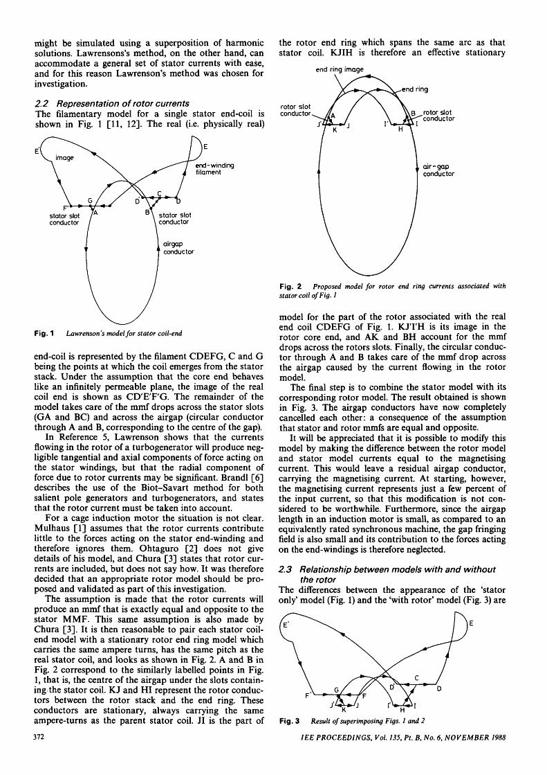
The first set of experimental results were taken withthe flux density probe sweeping through an arc close toboth rotor end ring and stator winding. The position ofthis arc is indicated at Test Position 1 in Fig. 6. Thevalues of the flux density coefficients, obtained by themethod described in the previous section, are shown ascircles in Figs. la-c. The design of the probe-holder wassuch that the measurements could be taken only over arestricted arc. The effective length of this arc wasincreased by exciting different phases of the winding, thenusing a spatial phase shift. This technique gave resultsover three overlapping arcs, with combined span of 220degrees.

test position 2 test position 1

rotor

rotor axis

Fig. 6 Projection of end-winding model on rz plane to show experi-mental measurement points

Figs, la-c also include the values of flux, density coef-ficients computed using the Biot-Savart Law, and modelswith and without representation of the rotor. The agree-ment between measured values and those computedusing the model which includes rotor currents is seen tobe very good in all three Figures. The model which doesnot include rotor currents gives equally good agreementfor the radial and circumferential flux coefficients, butpoor agreement for the axial coefficient.

300.00

200.00

10000

' 000

-10Q00

-200.00

-30000

with rotor

/ ^ j ^ . stator only

f \\ /

0.00 50.00 100.00 150.00 200.00 250.00 300.00 350.00 400.00

position, degrees

Fig. la Variation of<xr with circumferential position

Test position 1

374 IEE PROCEEDINGS, Vol. 135, Pt. B, No. 6, NOVEMBER 1988

A second set of experimental results was taken withthe probe close to the end-windings, but far from the

150.00

10000

x 50.00

=• -0.00

f-50.00

-100.00

-150 00

with rotor

.stator only

0.00 50.00 100.00 150.00 200.00 250.00 300.00 350.00 400.00position, degrees

Fig. 7b Variation ofag with circumferential position

Test position 1

20000

150.00

10000

50.00<

^_ 0.00

^ - 5 0 . 0 0

^-100.00

-150.00

-200.00

-250.00

-with rotor

0.00 50.00 10000 150.00 200.00 250.00 300.00 350.00400.00position, degrees

Fig. 7c Variation ofaz with circumferential position

Test position 1

core. The results obtained are shown in Figs. Sa-c whichrefer to an arc through test position 2 in Fig. 6. The com-puted curves show that the difference between the predic-tions made using the two models has diminished as thedistance from the core and end rings has increased. Thiswould be expected from considerations of the 'with rotor'model of Fig. 3 and the effective stator only model of Fig.4, which differ only in the region close to the core. Theagreement between computed and measured coefficientsin Figs. Sa-c is seen to be very good, once again showingthe overall validity of the Biot-Savart method.

The machine was then excited from a balanced three-phase supply, and tests carried out to determine the3-phase flux density coefficients. The results obtainedwith the probes swept through an arc through test posi-tion 1 (Fig. 6) are shown in Figs. 9a-c and \0a-c. The

60.00

40.00

< 20.00

^ -0.00

-20.00

-40.00

-60.000 00 50.00 100.00 150.00 200.00 250.00 30000 350XX) 400-00

position,degrees

Fig. 8a Variation ofar with position

Test position 2

'with rotor' predictions show good correlation with theexperimental results for all 3-phase flux density coeffi-cients, whilst the 'no rotor' model gives good results only

60.00 r .stator onlywith rotor / "

40.00

20.00<

^_ -Q00

CD

£-2000

- 40.00

- 60.000.00 50.00 100.00 150.00 200.00 250.00 300.00 350.00 40000

position, degrees

Fig. 86 Variation ofa$ with circumferential position

Test position 2

200.00

1 50.00

100.00

50.00

L ooor"-5o.oo-100.00

-150.00

-200.00

-with rotor-stator only

0.00 50.00 10Q00 150.00 200.00 250.00 300.00 350.00 400.00

position, degree

Fig. 8c Variation of<xz with circumferential position

Test position 2

450.00

400.00

350.00

300.00

; 250.00

^200.00

50.00

100.00

50.00

0.00

with rotor

stator only

0.00 50.00 100.00 150.00 200.00 250.00 300.00 350.00 400.00

position.degrees

Fig. 9a Variation ofar with circumferential position

Test position 1

250.00

200.00

^ 150.00

3.

' 100.00CD

50.00

00.00

with rotor

stator only

0.00 5000 100X50 150.00 200.00 250.00 300.00 350.00 400.00position, degrees

Fig. 9b Variation ofag with circumferential position

Test position 1

IEE PROCEEDINGS, Vol. 135, Pt. B, No. 6, NOVEMBER 1988 375

for the radial and circumferential coefficients, and a poorcorrelation for the axial coefficient. The calculated phasecoefficients, however, are seen to be in very good agree-

3 50.00 r

300.00

350.00

^ 200.00

^150.00

1 00.00

50.00

0.00

©«>

with rotor

stator only

0.00 50.00 100.00 150.00 200.00 250.00 300.00 350.00 400.00position, degrees

Fig. 9c Variation ofaz with circumferential position

Test position 1

-100.00

-150.00

-200.00

| -250.00

•8 -300.00a>o -350.00

-400.00

-450.00

-500.00

calculated variations1 (both models)

0.00 50.00 100.00 150.00 200.00 250.00 300.00 350.00 400.00position, degrees

Fig. 10a Variation ofQ>r with circumferential position

Test position 1

calculatedvariations(both models)

-200.000.00 50.00 100.00 150.00 200.00 250.00 300.00 350.00 400.00

position, degrees

Fig. 10b Variation o/<Dfl with circumferential position

Test position 1

100.00

5000

0D0

1 -50.00

ST"° -100.00a>2 -15000a.

200.00

250.00

300.00

with rotor

statoronly

0.00 50.00 100.00 150.00 200.00 250.00 30000 350.00 400.00position, degrees

Fig. 10c Variation ofQ>z with circumferential position

Test position 1

ment with the measured phase values, the results of thetwo models being virtually indistinguishable. Figs. 11 a-cand Yla-c repeat the above 3-phase results for an arc

45.00

40.00

35.00

30.00

^ 2 5.00

•J 0.00

$ 1 5.00

10.00

5.000.00

with rotorstator only

stator only with rotor

0.00 50.00 100.00 150.00 200.00 250.00 300.00 350.00 400.00position, degrees

Fig. 11a Variation ofar with circumferential position

Test position 2

80.00

70.00

60.00

< 50.00

=1:40.00

1^30.00

20.00

10.00

0.00

with rotor s ( Q ( o r Q n l y

0.00 50.00 100.00 150.00 200.00 250.00 300.00 350.00 400.00

position, degrees

Fig. 11b Variation ofae with circumferential position

Test position 2

200.00

180.00

160.00

140.00

I 120.00^ 100.00

i " 80.00

60.00

40.00

20D00.00

wi th rotor

stator only

0.00 50.00 100.00 150.00 200.00 25000 30000 35000 400.00position, degrees

Fig. 11c Variation ofuz with circumferential position

Test position 2

-50.00

-1 0.00

-150.00in

% -200.00en

•D -250.00

a -300.00

-350.00

-400.00-450.00

stator only

0.00 50.00 100.00 15000 200.00 250.00 300.00 35000 400.00

position, degrees

Fig. 12a Variation ofQ>r with circumferential position

Test position 2

376 IEE PROCEEDINGS, Vol. 135, Pt. B, No. 6, NOVEMBER 1988

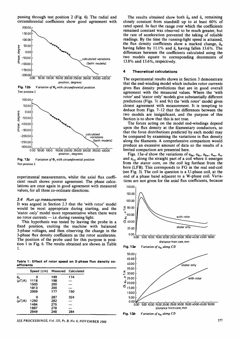
passing through test position 2 (Fig. 6). The radial andcircumferential coefficients show good agreement with

200.00

150.00

100.00

ft 50.00

? 0.00

-50.00

-100.00

-150.00

-200.00

__ calculated variations

(both models)

0.00 50.00 100.00 150.00 200.00 250.00 300.00 350.00 400.00

position, degrees

Fig. 126 Variation of<S>g with circumferential position

Test position 2

100.00

50.00

2 o.oo

§T -50.00

gj"-100.00

"E. -5000

-20000

-250.00

-300.00

calculatedvariations

Jboth models)

0.00 50.00 100.0 150.00 200.00 250.00 300.00 350.00 400.00position, degrees

Fig. 12c Variation of<J>x with circumferential position

Test position 2

experimental measurements, whilst the axial flux coeffi-cient result shows poorer agreement. The phase calcu-lations are once again in good agreement with measuredvalues, for all three co-ordinate directions.

3.4 Run up measurementsIt was argued in Section 2.3 that the 'with rotor' modelwould be most appropriate during starting, and the'stator only' model more representative when there wereno rotor currents — i.e. during running light.

This hypothesis was tested by leaving the probe in afixed position, exciting the machine with balanced3-phase voltages, and then observing the change in the3-phase flux density coefficients as the rotor accelerates.The position of the probe used for this purpose is posi-tion 1 in Fig. 6. The results obtained are shown in Table1.

Table 1: Effect of rotor speed on 3-phase flux density co-efficients

OTA)

ar

OTA)

Speed (r/m)

01118150018132969

01250148418872949

Measured

199198200200177

287282275278248

Calculated

174——

150

324———284

The results obtained show both ag and ar remainingclosely constant from standstill up to at least 60% ofrated speed. In fact the range over which the coefficientsremained constant was observed to be much greater, butthe rate of acceleration prevented the taking of reliablereadings. By the time the running-light speed is attained,the flux density coefficients show a marked change, a0having fallen by 11.1% and ar having fallen 13.6%. Thedifferences between the coefficients calculated using thetwo models equate to corresponding decrements of13.8% and 13.6%, respectively.

4 Theoretical calculations

The experimental results shown in Section 3 demonstratethat the end-winding model which includes rotor currentsgives flux density predictions that are in good overallagreement with the measured values. Where the 'withrotor' and 'stator only' models give substantially differentpredictions (Figs. 1c and 9c) the 'with rotor' model givesclosest agreement with measurement. It is tempting todeduce from Figs. 7-12 that the differences between thetwo models are insignificant, and the purpose of thisSection is to show that this is not true.

The forces acting on the model end-windings dependupon the flux density at the filamentary conductors, sothat the force distributions predicted by each model maybe compared by examining the variations in flux densityalong the filaments. A comprehensive comparison wouldproduce an excessive amount of data so the results of alimited comparison are presented here.

Figs. 13a-d show the variations of a0u, aBv, cc0w, <*„,, ccrvand arw along the straight part of a coil where it emergesfrom the stator core, on the coil leg furthest from thebore (LFB). This corresponds to FG in the real end-coil(see Fig. 3). The coil in question is a U-phase coil, at theend of a phase band adjacent to a W-phase coil. Varia-tions are not given for the axial flux coefficients, because

140.00

120.00

0.000.00 5.00 10.00 15.00 20.00 25.00 30.00 3500 40.00 4500 50.00

distance from core, mm

Fig. 13a Variation ofa^ along CD

50.00

45.00

40.00

35.00

2 30.00

^ 25.00

® 20.00

° 1 5.00

10.00

5.000.00

rotor

IEE PROCEEDINGS, Vol. 135, Pt. B, No. 6, NOVEMBER 1988

0.00 5.00 10.00 15.00 20.00 25.00 30.00 35.00 40.00 45.00 50.00distance from core, mm

Fig. 12b Variation ofaBv along CD

377

the axial flux produces no force, since the coil currentsthemselves are axially directed. The differences in coeffi-cients are shown to be large, showing that the twomodels will predicted different force distributions.

The differences between the flux-density coefficient dis-tributions predicted using the two models are smaller forparts of the coil that are far from the rotor end ring.

5.00

0.00

-5 00

10.00

.-15.00

-2000

-25.00

-30.00

stator only

with rotor

Fig. 13c

20.00

15.00

1000

£ 5.00

2 000

-500

-1000

0.00 5.00 10.00 1500 20.00 25.00 30.00 3500 40.00 45.00 50.00distance from core, mm

Variation o/a9w along CD

-15.00

Fig. 13d

0.00

-20.00

-40.00

P -60.00a.

> 80.00

-100.00

-120.00

0.00 5.00 10.00 15.00 20.00 25.00 30.00 35.0040.00 4500 50JOO

distance from core, mmVariation o/are along CD

-140.00

Fig. 13e

30Q00

250.00

200.00<

^-150.00

o 100.00

50.00

0.00

0.00 5.00 10.00 15.0020.0025.00 30.00 35.0040.00 45.00 50.00

distance from core, mmVariation ofan along CD

stator only

with rotor

0.00 5.00 10.00 15.00 20.0025.0030.00 35.0040.00 45.00 50.00

distance from core.mmFig. 13f Variation ofa^ along CD

Forces acting at points close to the coil nose enjoy alonger lever arm than those which act close to the core. Itmight appear, therefore, that the differences exhibited inFigs. 13a~d have little consequence. It will be appre-ciated, however, that the magnitude of the field is greatestclose to the core (cf Figs. 7-9 and 11), so that the short-ness of the lever arm is compensated for by an increase inthe force.

As further evidence that the diference between themodels is significant, the bending moments acting on thissame U-phase coil were examined. To do this it wasimagined that the coil is divided at the coil nose to givetwo mechanically separate coil halves, corresponding tothe LFB (leg from bore) and the LNB (leg nearest bore).Each coil leg is then regarded as being free to bend aboutthe three orthogonal axes which pass through the pointwhere it emerges from the stator core. For this (U-phase)coil, the bending moments may be expressed in a formsimilar to the flux density eqn. 2.

Mr

M2J

Pru

Peu

P,u

prvPev

Pzv

Prw

Pew

Pzw_

Vh

jw_

(10)

where Mr, M0 and Mz are the clockwise bendingmoments about the radial, circumferential and axial axespassing through the centre of the coil at the core end.The moment coefficients are calculated from the forcedistributions acting on the coil, as shown in Appendix 8.

Table 2 shows the moment coefficients calculated forthe two halves of the coil to which Figs. I3a-d relate. Itwill be seen that the more significant (i.e. larger) momentcoefficients, calculated using the two models, differ bybetween 10 and 25%. Furthermore, the differencesbetween the two models are not systematic. The 'withrotor' model will not always predict forces that aregreater than those predicted by the stator only model orvice versa.

Table 2: Comparison between moment coefficients actingon two coil halves

firuPr,Prw

PeuPe>Pew

P,uPnPm

I.FB

Stator only With rotor

634.1-92.9

1013.9

-107.2-9.6

-394.4

-21.9-24.0

-223.6

687.6-48.2888.1

-67.8-8.2

-457.2

9.1-24.7

-262.3

LNB

Stator only

1096.4-130.2

570.3

529.324.6

235.9

-248.45.7

-103.5

With rotor

984.9-62.4591.8

641.49.6

185.9

-298.712.3

-71.8

Units are Nm/A2 * 10'

5 Discussion and conclusions

A method for including the effect of rotor currents in thecalculation of end-winding forces using Lawrenson'sBiot-Savart method has been described, and shown topredict force distributions that are markedly differentfrom those obtained when rotor currents are ignored.Experimental measurements of flux coefficients haveshown that the new model is capable of predicting theflux distribution with good accuracy, and it may be sur-mised that the force distribution is therefore also reliablypredicted. The effect of rotor currents on the flux densitydistribution has also been demonstrated experimentally

378 1EE PROCEEDINGS, Vol. 135, Pt. B, No. 6, NOVEMBER 1988

by allowing the rotor to accelerate to running-lightspeed, and noting that the flux density coefficientsremained substantially constant until the running-lightspeed was achieved and the rotor current fell close tozero.

It should be pointed out that the experimental mea-surements were made on an open stator winding (i.e. withthe end cover removed) and with a pedestal bearing tosupport the rotor. Furthermore, the measurements weremade at the end of the machine that did not have thecooling fan. Both of these features mitigate in favour ofthe Biot-Savart method. On the other hand, the varia-tions in flux density coefficients measured and predictedin Figs. 7 and 8 indicate field distributions that are farfrom sinusoidal in the 0-direction, showing that the mainassumption made in the two-dimensional finite elementmethod must be carefully examined when transient con-ditions are being considered. Under steady-state condi-tions the sinusoidal assumption is equivalent to requiringvalues of the three-phase flux density coefficients (ar, ae,az) and linear variations in the phase coefficients (<fir, <f)0,(f>z). Reference to the measurements shown in Figs. 9 and11 show that the former requirement is suspect, whilst thephase measurements substantially support the latter.

6 Acknowledgments

The authors wish to thank the numerous members of theUK electrical machines industry with whom they sharedmany useful discussions during the course of this investi-gation. They would also like to thank Mr. M.J. Robin-son, who carried out the experimental work, and ShellUK Exploration and Production for both their supportand permission to publish this paper.

7 References

1 MULHAUS, J.: Transient forces on motor end-windings duringstart-up'. IEE Conf. Publ. No. 170, Conference on the design appli-cation and maintenance of large industrial drives, Savoy Place,London, 16-17 Nov., 1978, pp. 1-4

2 OHTAGURO, M., YAGIUCHI, K., and YAMAGUCHI, H.:'Mechanical behaviour of stator end windings', IEEE Trans. PowerAppar. & Syst., 1980, PAS-99, (3), pp. 1181-1185

3 CHURA, V., and POSMUROVA, E.: 'General Program for com-puting the forces in the end-windings of squirrel-cage inductionmotors', Ada Technica CSAV, 1980, 25, (4), pp. 406-430

4 PRICE, D.R., WALMSLEY, H.L., BUCKLEY, S., CLARK, P.E.,EWINS, D.J., ROBB, D.A., and WILLIAMSON, S.: 'Experimentalvalidation of a finite element method for predicting transient statorend-winding vibration in large electric motors'. IEE Conf. Publ. No.282, Third international conference on electrical machines anddrives, Savoy Place, London, 16-18 November 1987, pp. 106-112

5 LAWRENSON, P.J.: 'Forces on turbogenerator end windings',Proc. IEE, 1965,112, (6), pp. 1144-1158

6 BRANDL, P.: 'Forces on the end-windings of A.C. MACHINES',Brown-Boveri Rev., 1980,67, (2), pp. 128-134

7 PRESTON, T.W., and REECE, A.B.J.: "The contribution of thefinite-element method to the design of electrical machines: an indus-

trial viewpoint', IEEE Trans. Magn., 1983, MAG-19, (6), pp. 2375-2380

8 JACK, A.G., and MECROW, B.C.: 'Computation and validationagainst measurements of stator end-region fields in synchronousgenerators', IEE Proc. C, 1986,133, (1), pp. 26-32

9 SCOTT, DJ., SALON, S.J., and KUSIK, G.L.: 'Electromagneticforces on the armature end windings of large turbine generators,Part I — Steady-state', IEEE Trans. Power Appar. & Syst., 1981,PAS-100, (11), pp. 4597-4603

10 CLARK, P.E., and McSHANE, I.E.: 'Stator end-windingmovement-calculation and measurement'. IEE Conf. Publ. No. 213,International conference on electrical machines: design and applica-tions, Savoy Place, London, 13-15 July, 1982, pp. 1-5

11 CARPENTER, C.J.: The application of the method of images tomachine end-windings', Proc. IEE, 1960,107A, pp. 487-500

12 LAWRENSON, P.J.: 'The magnetic field of the end-windings ofturbo-generators', ibid., 1961,108A, pp. 538-549

8 Appendix

Calculation of moment coefficientsTo use the Biot-Savart law, it is convenient to divideeach filamentary coil model into elements and then tosum the effects of each interaction between the elements[5]-

Referring to Fig. 14, the current it in element 1 pro-duces a flux density dB at element 2. This flux interacts

dl.

Fig. 14 Interaction between current elements

with the current i2 to produce a force dF acting onelement 2. The force dF then contributes a moment dMacting about the point P. The required expressions are

dB =iY dltxr

An r3

dF = i2 dl2 x dB

dM = dF x r'

.Mjr Hohh dl2dll xr xdM = — 3

An r5

(11)

(12)

(13)

(14)

IEE PROCEEDINGS, Vol. 135, Pt. B, No. 6, NOVEMBER 1988 379