Inflation, Money Demand, and Purchasing PowerParity in South Africa

GUNNAR JONSSON*

This empirical study for South Africa indicates that there exists a stable moneydemand type of relationship among domestic prices, broad money, real income,and interest rates, as well as a long-run relationship among domestic prices,foreign prices, and the nominal exchange rate. In the short run, shocks to thenominal exchange rate affect domestic prices but have virtually no impact on realoutput, while shocks to broad money have a temporary impact on real outputbefore becoming inflationary. Both types of shocks seem to trigger a monetarypolicy response, as the short-term interest rate adjusts quickly. [JEL C32, E31,E41, F41]

South Africa adopted a formal inflation-targeting framework for monetarypolicy early in 2000, following less than satisfactory experiences with other

monetary policy regimes (such as an exchange rate peg and money growthtargeting, see Box 1) during the previous decades. The inflation target was set at3–6 percent by 2002, and transparency and accountability of the South AfricanReserve Bank (SARB) were enhanced.

The introduction of the new monetary policy regime was done in the contextof a considerable fall in inflation during the 1990s. Annual growth in the under-lying consumer price index fell from 18 percent in 1991 to 13 percent in 1993 andfurther to 7 percent in 1998. Developments in broad money (M3), however, did

243

IMF Staff PapersVol. 48, No. 2

© 2001 International Monetary FundMV

PY=

E ss

t t

−+1

PP

S=

*

QE

PV

QX

t

t

=

+(

)+1

yp

= + (β

1=

+( )F

i

S*

*

L Y i= ( ,

Y SPP

*, ,

ε ε+ >*

*Gunnar Jonsson is a Senior Economist at the International Monetary Fund. He wishes to thankTrevor Alleyne, Torbjörn Becker, David Coe, Neil Ericsson, José Fajgenbaum, Zenon Kontolemis,Michael Nowak, Jean-Claude Nachega, Eric Schalling, Arvind Subramanian, Yougesh Khatri, KrishnaSrinivasan, Carl Walsh, Tarik Yousef, and seminar participants at IMF’s African Department and theUniversity of Cape Town for discussions and comments. The usual disclaimer applies.

02 Jonsson 12/17/01 1:31 PM Page 243

Gunnar Jonsson

244

Box 1. Monetary and Exchange Rate Regimes in South Africa

The South African Reserve Bank has operated different monetary and exchange rate policyregimes during 1970–2000. This period has also witnessed a substantial degree of financial andexternal liberalization, where the latter included both trade reforms and capital controlliberalization.

1970–79: Between 1970–79, the rand was pegged to either the U.S. dollar or the poundsterling. However, frequent alterations to the level of the peg were undertaken in the form ofdiscrete step changes. The Reserve Bank also used changes in cash and liquid asset requirementscombined with credit ceilings and interest rate controls to affect liquidity conditions. At the sametime, exchange controls severely restricted the capital flows of residents, while nonresidents hadto place the proceeds from sales of South African assets in blocked rand accounts, which couldonly be freely transferred overseas after five years.

1980–85: A shift in the monetary policy regime took place in the early 1980s; the ReserveBank moved to a system of indirect control of money supply and adjustments of short-terminterest rates in an effort to enhance the responsiveness of monetary aggregates tomacroeconomic developments. Greater flexibility was also introduced into the foreign exchangeand capital markets. A managed float but dual exchange rate system was in place between1979–83, with financial transactions by nonresidents being valued at a discounted exchange rate(the “financial rand mechanism”), while current account transactions were valued at thecommercial exchange rate. The liberalization process continued between 1983–85, including theadoption of a unified exchange rate system, scaling down of liquid asset requirements, anddismantling of interest rate controls.

1985–94: In the context of the political upheavals in the mid-1980s, however, SouthAfrica declared a moratorium on most of its debt obligations in 1985, following the refusal by anumber of international banks to roll over short-term loans to South Africa. The ensuing financialsanctions resulted in a debt standstill and, subsequently, in a series of rescheduling agreementsbetween 1985–94. Moreover, the financial rand mechanism was reintroduced, and capital controlswere effectively tightened. Starting in 1986, the Reserve Bank announced target ranges forgrowth in broad money, which was lowered over time in an attempt to bring inflation down.Indeed, broad money growth and inflation fell substantially during this period, although theReserve Bank often missed the explicit money growth target.

1994–2000: Following the general elections in 1994, the new government intensified theliberalization efforts. The financial rand mechanism was terminated in 1995 and the exchangerate unified; capital controls on residents were gradually liberalized and virtually all controlson nonresidents were removed. Moreover, trade tariffs were lowered and exports and importsgrew sharply. At the same time, a substantial degree of financial deepening took place, as low-income households gained access to formal banking services to a larger extent. In this context,growth in broad money accelerated and exceeded the target ranges by wide margins every yearbetween 1994–99, but inflation was contained. The Reserve Bank emphasized that the moneygrowth target should be interpreted as an informal guideline. In practice, a more eclecticapproach was followed, which involved monitoring a number of different indicators, includingvarious price indices, the shape of the yield curve, the nominal exchange rate, and the outputgap. In February 2000, South Africa adopted a formal inflation-targeting framework formonetary policy.

Sources: Aron, Elbadawi, and Kahn (1997); Garner (1994); Moll (1999b); and the SouthAfrican Reserve Bank (1998).

02 Jonsson 12/17/01 1:31 PM Page 244

not follow the same pattern; although the annual growth rate of M3 fell from 14percent in 1991 to 5 percent in 1993, it increased to 17 percent in 1998. At thesame time, the nominal exchange rate has fluctuated widely in South Africa. Forexample, the nominal effective exchange rate depreciated on average by 61⁄2

percent a year between 1990 and 1995, but by 22 percent and 19 percent in 1996and 1998, respectively. The latter events were followed by a pickup in inflation,despite a tightening of monetary policy.

Issues related to the determinants and forecasting of inflation have assumedgreater importance under the inflation-targeting framework, including the impactof fluctuations in money and the nominal exchange rate. In particular, thecontrasting developments in inflation and money growth during the 1990s ledanalysts to question whether a stable relationship between these two aggregatesexists, and whether money demand is stable. At the same time, it has been notedthat movements in foreign prices and the nominal exchange rate are likely to havecontributed to inflation developments in South Africa, although the specifics ofsuch a relationship have not been examined thoroughly.1

The purpose of this study is to examine empirically the relationship amongprices, money, and the exchange rate in South Africa within a simple structuralsetting. More specifically, the study first examines the long-run stability of twoeconomic relationships involving the above-mentioned variables: a moneydemand type of relationship and purchasing power parity (PPP). Secondly, theshort-run responses and comovements among nominal and real variablesfollowing various types of shocks are investigated, with a particular focus on howinflation adjusts to these shocks. In the course of doing this, the issues of a poten-tial structural break in the data since 1994—the starting year of the successfulpolitical transformation of the economy and the lifting of sanctions—and whetherit is appropriate to focus on a more narrow or broader definition of money whenestimating money demand are tentatively examined.2

From a methodological perspective, it can be noted that the two long-run rela-tionships mentioned above are estimated simultaneously by using a structuralvector error-correction model (VECM). This contrasts with most of the literatureon PPP and money demand, where (error-correcting) single equation models areestimated. As both relationships involve domestic prices, however, it seemspreferable to model the interaction among the variables within a multivariate coin-tegration context.3

INFLATION, MONEY DEMAND, AND PURCHASING POWER PARITY IN SOUTH AFRICA

245

1It should be noted that South Africa remained a fairly open economy during the 1970s and 1980s,notwithstanding long periods of international trade and financial sanctions. For example, the sum ofmerchandise exports and imports remained at about 35 percent of GDP during the sanctions period1985–95, although the financial sanctions forced South Africa to shift from running external currentaccount deficits in the early 1980s to current account surpluses from 1985 to the early 1990s; see, forexample, Jonsson and Subramanian (2000) and Lipton (1998) for discussions.

2From a policy perspective, it would be important to also examine how several other variables—suchas wages, fiscal variables, and capacity utilization—are related to inflation developments in South Africa.This is, however, beyond the scope of the current paper.

3Becker (1999) and Price and Nasim (1999) are two recent studies that use a very similar method-ological approach to study the issues of PPP and money demand.

02 Jonsson 12/17/01 1:31 PM Page 245

The results indicate that there exists a stable and plausible money demandtype of relationship among domestic prices, broad money, real income, andinterest rates, as well as a long-run relationship among domestic prices, foreignprices, and the nominal exchange rate. In the short run, it is found that shocks tothe exchange rate affect domestic prices but have virtually no impact on realoutput. This contrasts with shocks to broad money, which have a temporaryimpact on real output before inflation picks up. Both types of shocks seem totrigger a monetary policy response, as the short-term interest rate adjusts quickly.

I. Background, Methodology, and Data

Empirical Background

The empirical literature on money demand and PPP is substantive, but in moststudies the focus is typically on only one of the two relationships.4 This is also thecase for South Africa. The most recent studies on the demand for money in SouthAfrica are Hurn and Muscatelli (1992) and Moll (1999a); both studies find asensible demand function for broad money despite a degree of financial innova-tion and liberalization in the 1980s and 1990s.5 This is corroborated by DeJagerand Ehlers (1997) who show that growth in M3 is a better and more stable indi-cator for future inflation rates than narrow money, and that M3 has a consistentnegative relationship with interest rates. These results contrast with Doyle (1996),who tentatively argues that narrow money (notes and coin in circulation outsidethe banking system) might warrant a more prominent role in the monetary policyframework, as this aggregate is a fair leading indicator for inflation, and as thedemand for narrow money appears to be stable.

Issues related to whether PPP holds in South Africa have been examined invarious papers. Tsikata (1998) and Subramanian (1998) show that the effectivenominal depreciation of the rand during the 1990s is almost fully reflected inhigher prices of imported goods, although the results are sensitive to the choice ofprice aggregates and sample period. This result does not necessarily mean thatPPP holds for national price levels. Indeed, Aron, Elbadawi, and Kahn (1997)argue that the real exchange rate in South Africa is nonstationary, implying that astrict interpretation of PPP would not hold. They show, however, that fluctuationsin the real exchange rate can be explained by variations in a set of economic“fundamentals,” including measures of trade liberalization, terms of trade, govern-ment expenditures, capital flows, and official reserves.

Gunnar Jonsson

246

4Johansen and Juselius (1990), Hendry and Ericsson (1991), and Ericsson (1998) are examples ofuseful studies that discuss a range of econometric and time-series issues that arises in studies of moneydemand. MacDonald (1995), Rogoff (1996), and Habermeier and Mesquita (1999) are examples ofstudies that survey the PPP literature and provide some new results using cointegration methods.

5Hurn and Muscatelli (1992) point out that a number of the earlier empirical studies on moneydemand in South Africa did not estimate the long-run elasticites in an econometrically satisfactory way.

02 Jonsson 12/17/01 1:31 PM Page 246

Theoretical Background

The theoretical underpinning for the study of money demand and PPP is stan-dard. The simplest form of the PPP theory suggests that goods market arbitrageenforces parity in national price levels. Hence, converted to a commoncurrency, national price levels should be equal, that is, all variables expressedin natural logarithms,

p = q – e , (1)

where p is the domestic price level, q represents (effective) foreign prices, and eis the nominal (effective) exchange rate (defined as foreign currency per domesticcurrency).6 At the same time, equilibrium in the money market implies that realmoney supply (ms – p) equals real money demand, with the latter assumed to apositive function of real income, y, and a negative function of the nominal interestrate, i,7 that is,

ms – p = md (y,i). (2)

Thus, we end up with a system of six interrelated variables [p, q, e, m, y, i],where economic theory suggests that two long-run relationships could befound: one between domestic prices, foreign prices, and the nominal exchangerate; and another between domestic prices, money, real income, and thenominal interest rate. While we would expect both the real exchange rate andreal money demand to be fairly stable in the long run, we would also expecttemporary deviations from these two long-run equilibria to affect future fluctu-ations in the variables such that the long-run equilibria are restored.

In addition to these considerations, a dummy variable for the period1994–98 was added to the model in an attempt to identify a possible structuralbreak associated with the economic effects of the political transformation thattook place in the early 1990s. This transformation, as well as some importanteconomic structural reforms, could have arguably affected both the long-runmoney demand relationship and the real exchange rate, since it led to both somefinancial deepening (as low-income households gained access to formalbanking services to a larger extent), as well as a strong increase in foreigncompetition, which in turn could have had a one-off effect on the domesticprice level.

INFLATION, MONEY DEMAND, AND PURCHASING POWER PARITY IN SOUTH AFRICA

247

6A variant of the simplest PPP hypothesis suggests that expression (1) should only hold for tradeablegoods, while prices for nontradables in part depends on relative productivity levels. The current studydoes not make a distinction between prices of tradables and nontradables.

7More precisely, economic theory suggests that demand for money depends on the opportunity costof holding money. Although the opportunity cost for holding cash is larger when the nominal interest rateis higher, it is ambiguous whether broader definitions of money are positively or negatively related to thenominal interest rate, as broad money typically is interest bearing. See the first part of Section II forfurther discussion.

02 Jonsson 12/17/01 1:31 PM Page 247

Data Issues and Econometric Methodology

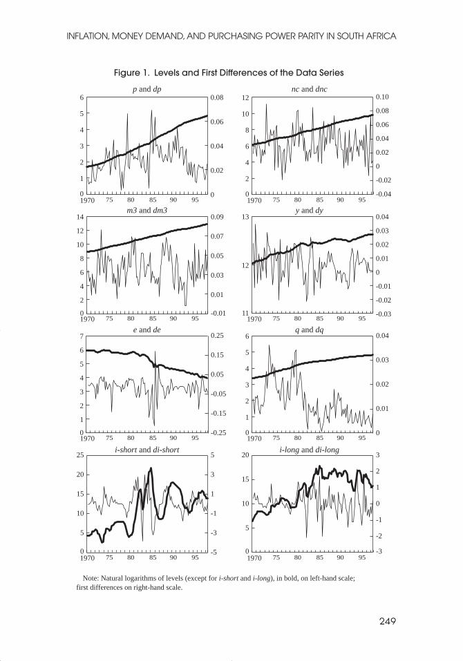
The empirical analysis was carried out using quarterly data between 1970:1 and1998:2. All series are plotted in Figure 1. The underlying consumer price index, p,was used rather than the headline consumer price index throughout the study. Byusing underlying inflation, which excludes highly volatile food prices and housingcosts (mainly mortgage costs) from the consumer price index, it was expected thatthe signal-to-noise ratio would improve in the estimations. To further examinewhether broad money or narrow money is more closely related to inflation, twodifferent monetary aggregates were used in the analysis: nc, notes and coin incirculation outside the banking sector; and m3 (broad money), consisting of ncplus check and demand deposits, and medium- and long-term deposits. Two alter-native interest rates were included in the model: a short-term rate (i-short) and along-term rate (i-long). The nominal exchange rate, e, and the foreign price level,q, were calculated in effective terms, using the Reserve Bank’s weights; anincrease in the effective nominal exchange rate means an appreciation of the rand.See Appendix for further data details.

Traditional unit root tests (see Table 1) indicated that all series are integratedof order 1, possibly with the exception of foreign prices, q, i.e., the series are non-stationary in levels but stationary in first differences.8 The nonstationarity of thedata together with the notion that none of the variables a priori can be regarded asexogenous, suggested that an appropriate methodology would be to start with anon-structural vector auto regression model (VAR), and use cointegration tests toexamine whether any long-run relationships exist among the variables.9 As asecond step, economic theory (as described above) was used for identification,turning the empirical model into a structural VAR, and specific cointegratingvectors—related to the PPP and money demand hypothesis—were estimated andtested. Hence, to allow for a dynamic interaction among the variables in thesystem, the two long-run relationships (as suggested by theory) were estimatedseparately but simultaneously, while no constraints were placed on the short-runadjustments.

More specifically, following Johansen and Juselius (1990) and Johansen(1991), a vector of endogenous variables, x, that are integrated of order 1, isanalyzed using the vector error-correction representation,

(3)∆ Γ ∆x x xt i t i t ti

k

= + + +− −=∑µ π ε1

1

,

Gunnar Jonsson

248

8Visual inspection suggests that a time trend arguably should be included in the first difference testfor q. Allowing for such a trend also indicates that this series is integrated of order 1. Moreover, theforeign price series adjusted for the effective exchange rate is clearly integrated of order 1.

9Foreign prices could arguably be treated as an exogenous variable. Indeed, as shown below, theempirical results reveal that foreign prices do not respond to deviations from the estimated long-run relationships.

02 Jonsson 12/17/01 1:31 PM Page 248

INFLATION, MONEY DEMAND, AND PURCHASING POWER PARITY IN SOUTH AFRICA

249

0

1

2

3

4

5

6

0

0.02

0.04

0.06

0.08

0

2

4

6

8

10

12

-0.04

-0.02

0

0.02

0.04

0.06

0.08

0.10

0

2

4

6

8

10

12

14

-0.01

0.01

0.03

0.05

0.07

0.09

11

12

13

-0.03

-0.02

-0.01

0

0.01

0.02

0.03

0.04

0

1

2

3

4

5

6

7

-0.25

-0.15

-0.05

0.05

0.15

0.25

0

5

10

15

20

25

-5

-3

-1

1

3

5

0

5

10

15

20

-3

-2

-1

0

1

2

3

0

1

2

3

4

5

6

0

0.01

0.02

0.03

0.04

1970 75 80 85 90 95 1970 75 80 85 90 95

1970 75 80 85 90 95 1970 75 80 85 90 95

1970 75 80 85 90 95 1970 75 80 85 90 95

1970 75 80 85 90 95 1970 75 80 85 90 95

p and dp nc and dnc

m3 and dm3 y and dy

e and de q and dq

i-short and di-short i-long and di-long

Note: Natural logarithms of levels (except for i-short and i-long), in bold, on left-hand scale; first differences on right-hand scale.

Figure 1. Levels and First Differences of the Data Series

02 Jonsson 12/17/01 1:31 PM Page 249

where the parameters µ and Γ1 ,…, Γk are allowed to vary without restrictions, kis the lag length of the model, and εt is a vector of normally distributed shockswith mean zero. The presence of cointegration is tested by examining the rank ofπ. In the event of reduced rank of π (that is, when rank (π) = r < n, where n is thenumber of endogenous variables), there exists r cointegrating vectors, and thematrix π can be written as π = αβ', with β containing the r cointegrating vectors,and α describing the speed of adjustments to the long-run equilibria (the error-correcting terms). If r > 1, the issue of identification arise. In the current paper, theexpected rank is 2, implying that (over)identifying restrictions should be placed onthe parameters in

(4)π

α αα αα αα αα αα α

β β β β β ββ β β β β β

x

p

q

e

m

y

i

t

t

−

−

=

1

11 12

21 22

31 32

41 42

51 52

61 62

11 12 13 14 15 16

21 22 23 24 25 26

1

.

Gunnar Jonsson

250

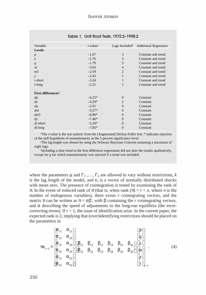
Table 1. Unit Root Tests, 1972:2–1998:2

Variable t-value1 Lags Included2 Additional RegressorsLevelsp –1.67 3 Constant and trende –2.76 3 Constant and trendq –1.79 5 Constant and trendnc –3.03 4 Constant and trendm3 –2.59 2 Constant and trendy –2.43 1 Constant and trendi-short –3.24 1 Constant and trendi-long –2.21 1 Constant and trend

First differences3

dp –6.23* 0 Constantde –4.29* 2 Constantdq –2.01 4 Constantdnc –9.27* 0 Constantdm3 –6.86* 0 Constantdy –7.46* 0 Constantdi-short –5.20* 0 Constantdi-long –7.85* 0 Constant

1The t-value is the test statistic from the (Augmented) Dickey-Fuller test; * indicates rejectionof the null hypothesis of nonstationarity at the 5 percent significance level.

2The lag length was chosen by using the Schwarz Bayesian Criterion assuming a maximum ofeight lags.

3Including a time trend in the first difference regressions did not alter the results qualitatively,except for q for which nonstationarity was rejected if a trend was included.

02 Jonsson 12/17/01 1:31 PM Page 250

In the estimations below, β11 and β21 will be normalized to 1, while the simplestforms of the PPP and money demand relationships will be tested by adding exclu-sion restrictions on [β14 β15 β16] and [β22 β23], respectively.

The short-run comovements among the variables are then examined by gener-ating orthogonalized impulse response functions (see Sims, 1980). As opposed tothe traditional VAR literature, however, the computation of the impulse responsefunctions is based on the VECM representation where the estimated long-runrestrictions are taken into account. This allows us to examine the effect of a vari-able-specific shock on the individual variables as well as on the estimated cointe-grating relationships; see Pesaran and Shin (1996). The main focus is on shocks tothe money, exchange rate, price, and output equations, respectively, in equation(4), with a special emphasis on the inflationary impacts of the different shocks. Itshould be emphasized that one has to be cautious in interpreting these shocks. Forexample, a shock to the money equation can originate from a number of differentsources, and does not necessarily mean that monetary policy has changed.Likewise, a shock to real output could be due to either an aggregate demand or anaggregate supply shock. See, for example, Becker (1999) for a discussion of theseidentification issues.

II. Results

Results Regarding the Long-Run Relationships

The results from the first set of cointegration tests are summarized in Table 2.The number of cointegrating vectors was estimated using the Johansen (1988,1991) procedure.10 It is well known that cointegration tests in the Johansensetting are sensitive to the lag-length of the VAR. Although it is common toinclude four lags in the VAR when quarterly data are used, at this stage, theresults are reported with two, three, and four lags included in the VAR, respec-tively.11 The economic model suggests that two cointegrating vectors shouldbe found (at least as long as only one interest rate is included in the model),and the cointegration tests typically picked up 2–3 stationary vectors (seeTable 2, Column 2). The results varied between zero and four vectors,however, depending on the number of lags included in the model, as well ason the choice of monetary aggregate and interest rate. Despite these somewhatinconclusive results, restricted cointegration tests were performed under theassumption of the presence of two cointegrated vectors. The parameters in therestricted model were constrained to test whether the two stationary vectors

INFLATION, MONEY DEMAND, AND PURCHASING POWER PARITY IN SOUTH AFRICA

251

10The number of cointegrating vectors was estimated using both the maximum eigenvalue statisticand the trace statistic (allowing for unrestricted intercepts but no trends), with the significance level set to5 percent.

11A time dummy for the period 1994:1–1998:2 and seasonal dummies were included in the model aswell. The time dummy was included without restricting it to the cointegrating vector, implying that theaverage growth rates of the variables can change at the time of the structural change, while the cointe-grating vectors remain unchanged.

02 Jonsson 12/17/01 1:31 PM Page 251

Gunnar Jonsson

252

Table 2. Structural VAR-Models, 1971:1–1998:21

Number of Chi-Square Statistic of Cointegrating Likelihood Ratio Tests of:3

Lags Vectors 2 PPP MD Joint Restricted Cointegrating Vectors 4

VAR-models including broad money, m3

p e q m3 y i-long i-short

2 1, 2 1.38 0.34 2.55 [ 1 0.89 –1.26 0 0 0 ]1 0 0 –0.76 1.14 –0.17

3 2, 2 2.02 0.61 4.65 [ 1 0.90 –1.26 0 0 0 ]1 0 0 –0.93 1.82 –0.11

4 2, 2 0.81 6.83** 7.87* [ 1 0.92 –1.26 0 0 0 ]1 0 0 –0.96 1.57 –0.10

2 3, 3 5.15 3.43 10.34* [ 1 0.87 –1.27 0 0 0 ]1 0 0 –1.11 1.72 0.02

3 3, 3 5.76 2.84 9.50* [ 1 0.91 –1.26 0 0 0 ]1 0 0 –1.08 1.43 0.03

4 1, 2 1.86 8.38** 12.28** [ 1 0.92 –1.12 0 0 0 ]1 0 0 –1.10 1.89 0.02

VAR-models including narrow money, nc

p e q nc y i-long i-short

2 2, 3 4.89 1.13 14.04** [ 1 0.93 –1.23 0 0 0 ]1 0 0 –1.18 0.68 0.15

3 2, 2 1.99 2.79 13.36** [ 1 0.95 –1.24 0 0 0 ]1 0 0 0.42 3.50 –1.46

4 1, 1 1.28 5.59* 16.14* [ 1 0.96 –1.22 0 0 0 ]1 0 0 –0.82 0.42 –0.26

2 4, 4 8.18* 5.54* 20.76** [ 1 0.87 –1.34 0 0 0 ]1 0 0 –0.98 0.07 0.01

3 4, 4 7.07* 0.09 7.59 [ 1 0.96 –1.21 0 0 0 ]1 0 0 –1.00 –0.04 0.02

4 0, 1 2.77 1.49 2.89 [ 1 0.91 –1.23 0 0 0 ]1 0 0 –0.96 –0.08 0.01

1The VAR also include (unrestricted) seasonal dummy variables and a time dummy for theperiod 1994:1–1998:2.

2Number of cointegrating vectors is based on Johansen’s Trace statistic and maximum eigen-value statistic, respectively, at the 5 percent significance level.

3* and ** indicate rejection of the LR-test at the 5 percent and 1 percent significance level,respectively.

4The estimations assume two cointegrating vectors. Bold figures are estimated coefficients.

02 Jonsson 12/17/01 1:31 PM Page 252

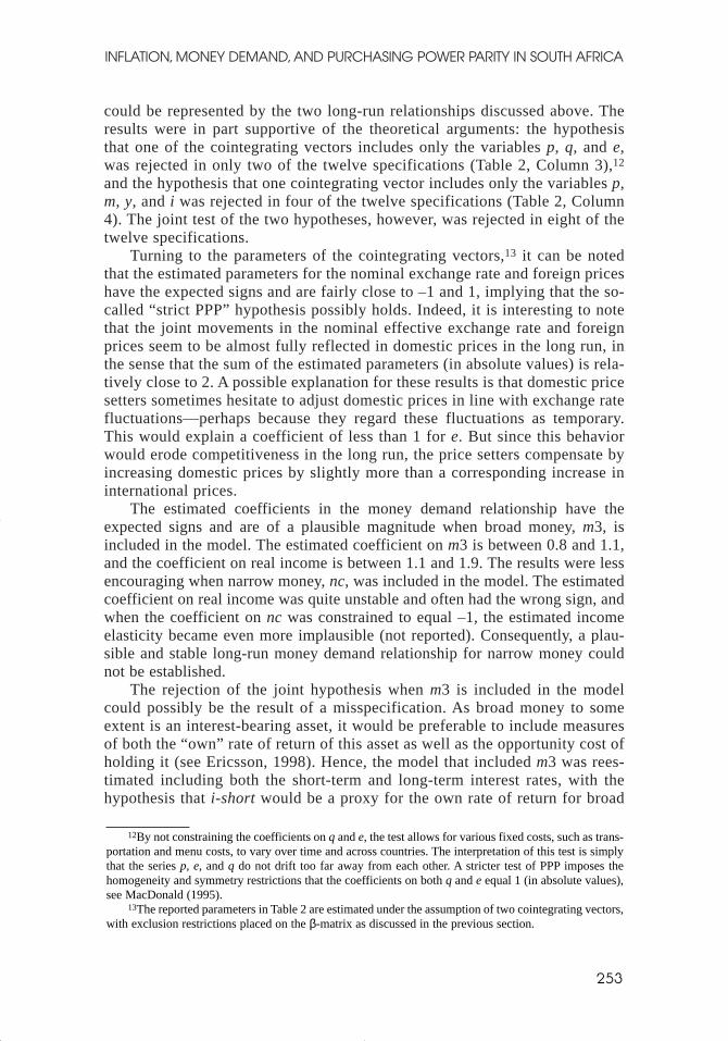
could be represented by the two long-run relationships discussed above. Theresults were in part supportive of the theoretical arguments: the hypothesisthat one of the cointegrating vectors includes only the variables p, q, and e,was rejected in only two of the twelve specifications (Table 2, Column 3),12

and the hypothesis that one cointegrating vector includes only the variables p,m, y, and i was rejected in four of the twelve specifications (Table 2, Column4). The joint test of the two hypotheses, however, was rejected in eight of thetwelve specifications.

Turning to the parameters of the cointegrating vectors,13 it can be notedthat the estimated parameters for the nominal exchange rate and foreign priceshave the expected signs and are fairly close to –1 and 1, implying that the so-called “strict PPP” hypothesis possibly holds. Indeed, it is interesting to notethat the joint movements in the nominal effective exchange rate and foreignprices seem to be almost fully reflected in domestic prices in the long run, inthe sense that the sum of the estimated parameters (in absolute values) is rela-tively close to 2. A possible explanation for these results is that domestic pricesetters sometimes hesitate to adjust domestic prices in line with exchange ratefluctuations—perhaps because they regard these fluctuations as temporary.This would explain a coefficient of less than 1 for e. But since this behaviorwould erode competitiveness in the long run, the price setters compensate byincreasing domestic prices by slightly more than a corresponding increase ininternational prices.

The estimated coefficients in the money demand relationship have theexpected signs and are of a plausible magnitude when broad money, m3, isincluded in the model. The estimated coefficient on m3 is between 0.8 and 1.1,and the coefficient on real income is between 1.1 and 1.9. The results were lessencouraging when narrow money, nc, was included in the model. The estimatedcoefficient on real income was quite unstable and often had the wrong sign, andwhen the coefficient on nc was constrained to equal –1, the estimated incomeelasticity became even more implausible (not reported). Consequently, a plau-sible and stable long-run money demand relationship for narrow money couldnot be established.

The rejection of the joint hypothesis when m3 is included in the modelcould possibly be the result of a misspecification. As broad money to someextent is an interest-bearing asset, it would be preferable to include measuresof both the “own” rate of return of this asset as well as the opportunity cost ofholding it (see Ericsson, 1998). Hence, the model that included m3 was rees-timated including both the short-term and long-term interest rates, with thehypothesis that i-short would be a proxy for the own rate of return for broad

INFLATION, MONEY DEMAND, AND PURCHASING POWER PARITY IN SOUTH AFRICA

253

12By not constraining the coefficients on q and e, the test allows for various fixed costs, such as trans-portation and menu costs, to vary over time and across countries. The interpretation of this test is simplythat the series p, e, and q do not drift too far away from each other. A stricter test of PPP imposes thehomogeneity and symmetry restrictions that the coefficients on both q and e equal 1 (in absolute values),see MacDonald (1995).

13The reported parameters in Table 2 are estimated under the assumption of two cointegrating vectors,with exclusion restrictions placed on the β-matrix as discussed in the previous section.

02 Jonsson 12/17/01 1:31 PM Page 253

money, while i-long would measure the rate of return of alternative assets.14 Atest for system reduction of the number of lags in the VAR indicated that fourlags should be included (the results are reported in Jonsson, 1999). The coin-tegration tests from this model are shown in Table 3. Both the maximumeigenvalue statistic and the trace statistic now indicate that there are threecointegrating vectors in the system. In addition to the two long-run relation-ships discussed above, it is conceivable that the two interest rates togetherform another long-run relationship—possibly along with domestic pricesand/or the exchange rate; the theory of the term structure of interest ratessuggests that a linear combination of long- and short-term interest ratescontains information about the future monetary policy stance and could helpin extracting expectations about future inflation rates and/or nominalexchange rate movements (see, for example, Mishkin, 1990). Although formaltests of, for example, the Fisher hypothesis or an examination of the termstructure of interest rates is beyond the scope of this paper, it is still possibleto test the joint hypothesis about the two vectors relating to the PPP andmoney demand relationships and still allow for the existence of a third cointe-grating vector.15

The results with regard to the money demand and PPP type of relationships werenow supportive of the theoretical arguments. The joint test of the hypothesis that twoof the three cointegrating vectors can be represented by a money demand and PPPtype of relationship could not be rejected (see Table 3), and the estimated coefficientshad the expected sign and were of plausible magnitudes. A visual inspection of thetwo restricted cointegrating vectors (denoted CVppp and CVmd) further indicates thatthese vectors seem to be reasonably stationary, see Figure 2 and Table 4.16

Regarding the PPP relationship, the unconstrained coefficients on e and q areestimated to 0.95 and –1.19. Constraining the coefficient on q to –1, effectivelyestimating how the nominal effective exchange rate relates to price differentials inthe long run, yielded an estimated coefficient on e of 1.06, which is not signifi-cantly different from 1. Put differently, the model where the coefficients on e andq were constrained to 1 and –1, respectively, was not rejected.

The estimated coefficients in the money demand type of relationship were alsoquite sensible. Long- and short-term interest rates entered the vector with differentand predicted signs; that is, higher short-term rates are positively related to realmoney balances (indicating a higher demand for broad money, the higher the ownrate of return), whereas higher long-term rates are negatively related to real money

Gunnar Jonsson

254

14The short-term interest rate refers to the three-month T-bill rate. Although a preferable measure ofthe own rate of return would be the actual bank deposit rate, such a series exists only since 1978.Nevertheless, the T-bill rate seems to be a good proxy for the own rate of return, as it is highly correlatedwith the deposit rate; indeed, the correlation coefficient between the two interest rate series is 0.95 for theperiod 1978–98.

15In fact, Podivinsky (1998) shows that it is preferable to overspecify the number of variables in themodel and later add exclusion restrictions, rather than underspecifying the model, as the latter has lowpower in detecting the true number of cointegrating vectors.

16The restricted cointegrated vectors in Figure 2 are given by the fourth specification in the lower partof Table 4, that is, CVppp = [p + 0.88*e – 1.28*prow] and CVmd = [p – m3 + 1.22*y – 0.04*i-long + 0.02*i-short].

02 Jonsson 12/17/01 1:31 PM Page 254

balances (indicating a lower demand for money, the higher the rate of return on thealternative asset). Moreover, constraining the coefficient on m3 to –1 yields an esti-mated income elasticity of 1.22. This coefficient is not significantly different from1 but is significantly different from 0.5. Hence, the long-run income elasticity forbroad money seems to be greater than 0.5 but not significantly different from unity.

Recursive estimations of the long-run parameters (the restricted cointegrationvectors) further show that the estimated coefficients are quite stable. Figure 3 plotsrecursive estimates of the coefficients for the nominal effective exchange rate, e,

INFLATION, MONEY DEMAND, AND PURCHASING POWER PARITY IN SOUTH AFRICA

255

Table 3. Cointegration Analysis of PPP and Demand for Broad Money

Rank Eigenvalue Lambda Critical Value (95%) Trace Critical Value (95%)r = 0 0.48 72.34** 45.3 189.6** 124.2r <= 1 0.32 42.72* 39.4 117.2** 94.2r <= 2 0.28 36.71* 33.5 74.49* 68.5r <= 3 0.20 24.24 27.1 37.79 47.2r <= 4 0.07 8.02 21.0 13.54 29.7r <= 5 0.05 5.35 14.1 5.53 15.4r <= 6 0.00 0.18 3.8 0.18 3.8

Joint TestRestricted Cointegrating Vectors1 Chi-Square2

p e q m3 y i-long i-short

[ 1 0.95 –1.19 0 0 0 0 ] 0.881 0 0 –1.07 1.72 –0.02 0.02

[ 1 1.06 –1 0 0 0 0 ] 6.021 0 0 –1.09 1.88 –0.02 0.02

[ 1 1 –1 0 0 0 0 ] 7.261 0 0 –1.08 1.83 –0.02 0.02

[ 1 0.88 –1.28 0 0 0 0 ] 6.571 0 0 –1 1.22 –0.04 0.02

[ 1 0.88 –1.34 0 0 0 0 ] 7.911 0 0 –1 1 –0.04 0.02

[ 1 0.89 –1.52 0 0 0 0 ] 12.72*1 0 0 –1 0.5 –0.05 0.02

[ 1 1 –1 0 0 0 0 ] 17.74**1 0 0 –1 1 –0.03 0.03

Notes: Endogenous variables: [p, e, q, m3, y, i-long, i-short], four lags includedUnrestricted variables: [Seasonal dummies, Time-dummy 1994:1–1998:2]Time period: 1971:1–1998:2 (110 observations)1The estimations assume three cointegrating vectors, where the third vector is unconstrained.

Bold figures are estimated coefficients.2* and ** indicate rejection of the joint likelihood ratio test at the 5 percent and 1 percent

significance level, respectively.

02 Jonsson 12/17/01 1:31 PM Page 255

Gunnar Jonsson

256

1970 75 80 85 90 95

3.0

2.5

2.0

1.5

3.5

1.0

Figure 2. Restricted Cointergration Vectors

Restricted cointegrating vector: CVppp

1970 75 80 85 90 95

7.3

7.1

6.9

6.7

7.5

6.5

Restricted cointegrating vector: CVmd

Table 4. Weak Exogeneity Tests

Only restrictions on β: Chi-sq (3): 6.57

Additional α restrictions:q (CVmd and CVppp) = 0 Chi-sq (2): 0.00

p (CVppp) = 0 Chi-sq (1): 14.18**e (CVppp) = 0 Chi-sq (1): 4.94*p (CVmd) = 0 Chi-sq (1): 0.24m3 (CVmd) = 0 Chi-sq (1): 2.89y (CVmd) = 0 Chi-sq (1): 0.18i-long (CVmd) = 0 Chi-sq (1): 0.29i-short (CVmd) = 0 Chi-sq (1): 5.26*

1Standard errors in parentheses. The symbols * and ** indicate rejection of the test at the 5 percent and 1percent significance level, respectively.

Restricted Cointegrating Vectors (β matrix)p e q m3 y i-long i-short1 0.88 –1.28 0 0 0 01 0 0 –1 1.22 –0.04 0.02

0.99 0.32 –0.90 –0.68 2.41 0.01 0.01

Adjustment Matrix (α matrix)1

p e q m3 y i-long i-short–0.05 –0.25 0 –0.09 0.04 2.43 5.88(0.02) (0.10) — (0.03) (0.02) (1.29) (1.50)

0.01 0.33 0 0.11 –0.02 1.34 –10.08(0.03) (0.18) — (0.05) (0.03) (2.29) (2.66)

–0.03 –0.23 –0.05 0.15 –0.17 –4.31 6.96(0.04) (0.20) (0.01) (0.06) (0.04) (2.71) (3.14)

02 Jonsson 12/17/01 1:31 PM Page 256

and real income, y, including ± 2 standard errors. The recursive initial lag lengthwas chosen to 65, leading to a minimum time span of about 16 years. The coeffi-cient on q was constrained to –1 in the PPP relationship, implying that the coeffi-cient on e is an estimate of the long-run relationship between the nominal effectiveexchange rate and price differentials. Although there are indications of a smallbreak in the relationship around 1992–93, the estimated coefficients of e areremarkably stable around 1. This further strengthens the result that the PPPhypothesis is a reasonable description of the long-run relationship between devel-opments in the nominal exchange rate and inflation differentials. With regard tothe recursively estimated coefficient on y, it is fairly stable around 1.5, althoughthere are indications of an upward trend break during the late 1990s.17

Short-Run Dynamics

Thus far, the results show that the variables in the model tend to move together inthe long run as predicted by economic theory. To draw policy conclusions,however, the issues of whether the variables should be treated as exogenous orendogenous and how they interact in the short run become important. More gener-ally, it is often useful to examine how the economy adjusts toward the long-run

INFLATION, MONEY DEMAND, AND PURCHASING POWER PARITY IN SOUTH AFRICA

257

17The recursive estimations occasionally failed to converge due to the sharp reductions in the numberof observations. Hence, these estimations were done under the assumption of two (rather than three) cointe-grating relationships, and without constraining the coefficient on m3 to –1. Nevertheless, the estimated coef-ficient on m3 was always relatively close to –1; the fact that it was not constrained to this value implies thatthe recursively estimated coefficient on y is a somewhat (upward) biased estimate of the income elasticity.

1987 89 91 93 95 97

1987 89 91 93 95 97

Figure 3. Recursive Cointegration Results(point estimates and +/–2 standard errors)

0.8

0.9

1.0

1.1

1.2beta-e

beta-y

0.5

1.0

1.5

2.0

2.5

02 Jonsson 12/17/01 1:31 PM Page 257

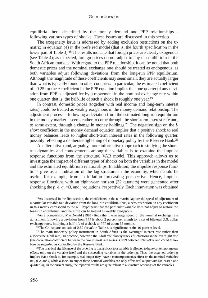
equilibria—here described by the money demand and PPP relationships—following various types of shocks. These issues are discussed in this section.

The exogeneity issue is addressed by adding exclusion restrictions on the α-matrix in equation (4) in the preferred model (that is, the fourth specification in thelower part of Table 3).18 The results indicate that foreign prices are clearly exogenous(see Table 4); as expected, foreign prices do not adjust to any disequilibrium in theSouth African markets. With regard to the PPP relationship, it can be noted that bothdomestic prices and the nominal exchange rate should be treated as endogenous, asboth variables adjust following deviations from the long-run PPP equilibrium.Although the magnitude of these coefficients may seem small, they are actually largerthan what is typically found in other countries. In particular, the estimated coefficientof –0.25 for the e coefficient in the PPP equation implies that one quarter of any devi-ation from PPP is adjusted for by a movement in the nominal exchange rate withinone quarter, that is, the half-life of such a shock is roughly one year.19

In contrast, domestic prices (together with real income and long-term interestrates) could be treated as weakly exogenous in the money demand relationship. Theadjustment process—following a deviation from the estimated long-run equilibriumin the money market—seems rather to come through the short-term interest rate and,to some extent, through a change in money holdings.20 The negative sign on the i-short coefficient in the money demand equation implies that a positive shock to realmoney balances leads to higher short-term interest rates in the following quarter,possibly reflecting a deliberate tightening of monetary policy by the Reserve Bank.21

An alternative (and, arguably, more informative) approach to studying the short-run dynamics and comovements among the variables is to examine the impulseresponse functions from the structural VAR model. This approach allows us toinvestigate the impact of different types of shocks on both the variables in the modeland the estimated equilibrium relationships. In addition, the impulse response func-tions give us an indication of the lag structure in the economy, which could beuseful, for example, from an inflation forecasting perspective. Hence, impulseresponse functions with an eight-year horizon (32 quarters) were generated aftershocking the p, e, q, m3, and y equations, respectively. Each innovation was obtained

Gunnar Jonsson

258

18As discussed in the first section, the coefficients in the α-matrix capture the speed of adjustment ofa particular variable to a deviation from the long-run equilibria; thus, a zero restriction on any coefficientin this matrix correspond to the null hypothesis that the particular variable does not adjust to restore thelong-run equilibrium, and therefore can be treated as weakly exogenous.

19As a comparison, MacDonald (1995) finds that the average speed of the nominal exchange rateadjustment following a deviation from PPP is about 2 percent per month for a set of bilateral U.S. dollarexchange rates, implying a half-life of a shock to PPP of about 36 months.

20The Chi-square statistic of 2.89 for m3 in Table 4 is significant at the 10 percent level.21The main monetary policy instrument in South Africa is the overnight interest rate rather than

i-short (the T-bill rate). In practice, however, the T-bill rate closely tracks fluctuations in the overnight rate(the correlation coefficient between the two interest rate series is 0.99 between 1970–98), and could there-fore be regarded as controlled by the Reserve Bank.

22The practical significance of the ordering is that a shock to a variable is allowed to have contemporaneouseffects only on the variable itself and the succeeding variables in the ordering. Thus, the assumed orderingimplies that a shock to, for example, real output may have a contemporaneous effect on the nominal variablesm3, p, e, and i, while a shock to any of these nominal variables can only affect real output with (at least) a onequarter lag. In the current study, the reported results are quite robust to alternative orderings of the variables.

02 Jonsson 12/17/01 1:31 PM Page 258

by a standard Choleski decomposition, where the ordering of the variables, ingeneral, matters. Somewhat arbitrarily the chosen ordering was q, y, m3, p, e, i-short,and i-long.22

The results are illustrated in Figures 4 and 5. To start with, a deviation fromthe long-run PPP relation can occur due to a shock to the nominal exchange rate,domestic prices, or foreign prices. The impacts of shocks to these equations areshown in Figure 4; the left-hand panels show the adjustments over time of someselected individual variables, while the right-hand panels show the developmentsof the deviations from the estimated long-run PPP equilibrium.

A positive shock to domestic prices will lead temporarily to an appreciation ofthe real exchange rate. The nominal exchange rate, however, will start to depre-ciate sharply already after three to four quarters, peaking after about eight quar-ters. In fact, the response of the exchange rate will be sufficiently sharp to causean overshooting effect leading to a temporary real depreciation before equilibriumis restored, as illustrated in the dynamic effects on the cointegrating vector.

Likewise, a shock to the nominal exchange rate, say a depreciation (a negativeshock), will almost immediately result in higher inflation. The half-life time ofsuch a shock seems to be about five quarters, a result that is in line with the earlierresult from the α-matrix. The effect on real output from a shock to the e equationis plotted in the middle (left) panel. It is interesting to note that, although a shockto the nominal exchange rate leads to a quite persistent effect on the real exchangerate (the real exchange rate remains, say, depreciated for several years before fulladjustment takes place), the impact on real output is virtually zero.

Finally, a shock to foreign prices will cause domestic prices to respond (asearlier noted). Nevertheless, the real exchange rate will temporarily deviate fromthe long-run equilibrium, as the nominal exchange rate also adjusts. The responseof domestic prices peaks after about eight quarters, before the variables settle ona new path to restore equilibrium.

Turning to the short-run comovements of the variables in the money demandfunction, the left-hand panels in Figure 5 show the dynamic effect of a one stan-dard error shock to the m3 equation. Again, it should be noted that a shock tomoney can originate from different sources and should not necessarily be inter-preted as a monetary policy shock. Nevertheless, it is interesting that, in contrastto a shock to the nominal exchange rate, a positive shock to money leads to aninitial but temporary output gain that peaks after about one year. The excessmoney balances also seem to trigger a tightening of monetary policy, however, asthe short-term interest rate picks up sharply after a couple of quarters. Theseeffects also imply that the cointegrating relationship is driven back toward itsequilibrium as higher real balances are offset by higher output and higher short-term interest rates. Domestic prices start to pick up after about five to six quarters,implying that real money balances adjust back toward their initial level at the sametime as the output effect vanishes and equilibrium is restored. One can also noticethat long-term interest rates pick up after a couple of quarters, indicating that infla-tion expectations (correctly) rise.

Finally, a positive shock to real output leads quickly to higher demand for realbalances and holding of broad money rises. The expected impact on domestic

INFLATION, MONEY DEMAND, AND PURCHASING POWER PARITY IN SOUTH AFRICA

259

02 Jonsson 12/17/01 1:31 PM Page 259

Gunnar Jonsson

260

0 5 10 15 20 25 30

0.01

0

–0.01

–0.02

–0.03

–0.04

0.02

p

e

–0.05

Figure 4. Impulse Responses of Shocks to the PPP Relation

One standard error shock in the p equation

0 5 10 15 20 25 30

1.50

1.00

0.50

0

–0.50

–1.00

–1.50

2.00

CVppp

–2.00

One standard error shock in the p equation

0 5 10 15 20 25 30

0.80

0.60

0.40

0.20

1.00

CVppp

CVppp

0

One standard error shock in the e equation

0 5 10 15 20 25 30

5.00

4.00

3.00

2.00

1.00

0

6.00

–1.00

One standard error shock in the q equation

0 5 10 15 20 25 30

0.04

0.02

0

–0.02

0.06

p

p

e

e

y

q

–0.04

One standard error shock in the e equation

0 5 10 15 20 25 30

0.03

0.02

0.01

0.04

0

One standard error shock in the q equation

02 Jonsson 12/17/01 1:31 PM Page 260

INFLATION, MONEY DEMAND, AND PURCHASING POWER PARITY IN SOUTH AFRICA

261

Figure 5. Impulse Responses of Shocks to the Money Demand Relation

0 5 10 15 20 25 30

One standard error shock in the y equation

0 5 10 15 20 25 30

1.00

0.80

0.60

0.40

0.20

1.20

y

CVmd

CVmd

0

One standard error shock in the y equation

0 5 10 15 20 25 30

0.50

0

–0.50

–1.00

1.00

–1.50

One standard error shock in the y equation

0 5 10 15 20 25 30

0.80

0.60

0.40

0.20

0

1.00

m3

i-short i-short

i-long

i-long

p

m3

y

p

m3

y

–0.20

One standard error shock in the m3 equation

0 5 10 15 20 25 30

–0.20

–0.60

–0.40

–0.80

–1.00

0

–1.20

One standard error shock in the m3 equation

0 5 10 15 20 25 30

0.03

0.02

0.01

0.04

0

0.03

0.02

0.01

0.04

0

One standard error shock in the m3 equation

02 Jonsson 12/17/01 1:31 PM Page 261

prices is in principle ambiguous, as it depends on whether the output shock isdriven by a shift in aggregate demand or aggregate supply. The empirical resultsindicate, however, that a positive shock to output results in inflationary pressuresafter about four to five quarters; although there will initially be some downwardpressure on domestic prices, the end effect is a higher price level. Again, themagnitude of these inflationary pressures seems to be mitigated by a tightening ofmonetary policy, as short-term interest rates rise.

The above results are similar to what is found in a number of other countries.For example, Sims (1992) uses a similar VAR setup to study the effects of mone-tary policy in five OECD countries. He shows that a shock to the money equationresults in a temporary real output response in France, the United Kingdom, and theUnited States, while inflation adjusts with a lag. He also shows that a positiveshock to real output results in upward pressure on domestic prices in several coun-tries. Likewise, Eichenbaum (1992) shows that a positive shock to money (M1)results in a small and temporary increase in output in the United States, but alsoin a sharp and substantial adjustment in the short-term interest rate (the federalfunds rate), while domestic prices pick up gradually and peak after about four tofive quarters.

III. Discussion and Conclusions

The results in this paper indicate: (i) a stable money demand type of relationshipexists among domestic prices, broad money, real income, and nominal interestrates, with plausible estimates of the long-run coefficients, as well as a long-runrelationship among domestic prices, foreign prices, and the nominal effectiveexchange rate; and (ii) in the short run, shocks to the exchange rate affect domesticprices but have virtually no impact on real output, while shocks to broad moneyhave a temporary impact on real output before inflation picks up. Both types ofshocks seem to trigger a monetary policy response, as the short-term interest rateadjusts quickly and substantially.

An interesting aspect of the results is that even though the South Africaneconomy has undergone a number of important structural changes during thestudied period—including long periods of trade sanctions, the presence of thefinancial rand system and widespread exchange controls on residents, differentmonetary policy regimes (see Box 1), and considerable swings in the terms oftrade—the long-run relationships among the examined macroeconomic and finan-cial aggregates are fairly stable and consistent with economic theory. In thiscontext, it is perhaps not surprising that it is the broadest measure of money thatseems to work better in the long run, as the more narrow money aggregatespossibly would exhibit more frequent structural breaks.

The result with regard to the PPP relationship is, perhaps, somewhatsurprising. Although considerable evidence for other countries suggests that thereal exchange rate is mean-reverting in the long run, especially for small openeconomies with floating exchange rates (see MacDonald and Marsh, 1997; andRogoff, 1996), homogeneity and symmetry restrictions are often rejected, anddeviations from PPP tend to dampen out only at a relatively slow rate. Also, as

Gunnar Jonsson

262

02 Jonsson 12/17/01 1:31 PM Page 262

noted earlier, Aron, Elbadawi, and Kahn (1997) find that the real exchange rate inSouth Africa is non-stationary but cointegrated with a set of “fundamentals.”

In the current study, the results clearly show that domestic prices, foreignprices, and the nominal exchange rate form a cointegrated vector in South Africa.Moreover, the estimated coefficients of this vector are relatively close to unity (inabsolute terms), although a strict test of PPP is rejected in some specifications.When comparing these results to the ones in Aron, Elbadawi, and Kahn (1997), itis important to note that the current study allows for a structural break in 1994.23

This break is intended to capture the opening up of the South African economy inrecent years, which have included a significant degree of trade liberalization (seeJonsson and Subramanian, 2000) as well as financial deepening. Indeed, Aron,Elbadawi, and Kahn (1997) find that various measures of trade liberalization is animportant determinant of the real exchange rate and note, for example, that thereduction of tariffs since 1994 is consistent with a more depreciated real exchangerate. These findings would thus be in line with the results in the current study.

Aron, Elbadawi, and Kahn (1997) also argue that the South African ReserveBank appears to have actively stabilized the real exchange rate during certainperiods, in which case the PPP finding in the current study rather should be inter-preted as a policy reaction function. It should also be emphasized that the findingsin this paper do not preclude deviations in the real exchange rate from its equilib-rium level from time to time with potentially damaging effects on South Africa’scompetitiveness.

With regard to the money demand relationship, it is interesting to note thatnotwithstanding the structural changes mentioned above, the magnitude andpattern of the estimated relationship is similar to what is found in many otherindustrial countries. Both the estimation of a long-run income elasticity close to 1and the estimated short-run comovements among the variables are in line with theempirical results found for many other countries, see Fase (1993) and Sims(1992), respectively. For example, the results that shocks to either money or outputaffect domestic prices with a lag of four to six quarters is similar to what is foundin several other inflation-targeting countries. Taken together, these results suggestthat it would be possible to develop a satisfactory forecasting model for inflationin South Africa, which is similar to the ones used in other countries that haveadopted an inflation-targeting framework for monetary policy.

INFLATION, MONEY DEMAND, AND PURCHASING POWER PARITY IN SOUTH AFRICA

263

23It should also be noted that the definitions of domestic prices are different (the current study uses“underlying CPI,” whereas Aron, Elbadawi, and Kahn (1997) use wholesale price index) and that theexamined time period is somewhat different.

02 Jonsson 12/17/01 1:31 PM Page 263

APPENDIX

Unless otherwise indicated, the data series are from the South African Reserve Bank (SARB),Quarterly Bulletin.p: Underlying consumer price index. This index was provided by the SARB for 1975–98, andequals headline consumer price index excluding “food and non-alcoholic beverages,” “homeowner’s cost” and “value-added tax.” For 1970–75, the series was defined as the headlineconsumer price index net of food prices.nc: Notes and coins outside the banking system.m3: nc plus checking deposits, and short-, medium-, and long-term deposits.i-short: Interest rate on three-month T-bills. Source: International Financial Statistics (IFS),IMF.i-long: Interest rate on ten-year government bonds. Source: IFS, IMF.e: Nominal effective exchange rate including (weights in brackets) U.S. dollar (51.7), poundsterling (20.2), deutsche mark (17.2), and Japanese yen (10.9).q: Effective consumer price index in foreign countries, including the same four countries andweights as when calculating e. Source: IFS, IMF.y: Gross domestic product, 1990 prices, seasonally adjusted.

REFERENCES

Aron, J., I. Elbadawi, and B. Kahn, 1997, “Determinants of the Real Exchange Rate in SouthAfrica,” Working Paper, WPS/97–16 (Oxford: Oxford University, Centre for the Study ofAfrican Economies).

Becker, T., 1999, “Common Trends and Structural Change: A Dynamic Macro Model for Pre-and Post-Revolution Iran,” IMF Working Paper 99/82 (Washington: International MonetaryFund).

DeJager, C. J., and R. Ehlers, 1997, “The Relationship Between South African MonetaryAggregates, Interest Rates, and Inflation—A Statistical Investigation” (unpublished;Johannesburg: South African Reserve Bank, Economics Department).

Doyle, P., 1996, “Narrow Monetary Aggregates,” in South Africa: Selected Economic Issues,IMF Staff Country Reports 96/64 (Washington: International Monetary Fund).

Eichenbaum, M., 1992, “Interpreting the Macroeconomic Time Series Facts: The Effects ofMonetary Policy,” European Economic Review, Vol. 36, pp. 1001–11.

Ericsson, N., 1998, “Empirical Modeling of Money Demand,” Empirical Economics, Vol. 23,pp. 295–315.

Fase, M. M. G., 1993, “The Stability of the Demand for Money in the G-7 and EC Countries:A Survey,” Research Memorandum WO & E 9321 (Amsterdam: De Nederlandsche Bank).

Garner, J., 1994, “An Analysis of the Financial Rand Mechanism,” Research Paper 9 (London:London School of Economics, Centre for Research into Economics and Finance in SouthAfrica).

Habermeier, K. F., and M. Mesquita, 1999, “Long-Run Exchange Rate Dynamics: A Panel DataStudy,” IMF Working Paper 99/50 (Washington: International Monetary Fund).

Hendry, D., and N. Ericsson, 1991, “Modeling the Demand for Narrow Money in the UnitedKingdom and the United States,” European Economic Review, Vol. 35, pp. 833–86.

Hurn, A. S., and V. A. Muscatelli, 1992, “The Long-Run Properties of the Demand for M3 inSouth Africa,” South African Journal of Economics, Vol. 60, No. 2, pp. 159–72.

Gunnar Jonsson

264

02 Jonsson 12/17/01 1:31 PM Page 264

Johansen, S., 1988, “Statistical Analysis of Cointegrating Vectors,” Journal of EconomicDynamics and Control, Vol. 12, No. 2/3, pp. 231–54.

———, 1991, “Estimation and Hypothesis Testing of Cointegrating Vectors in Gaussian VectorAutoregressive Models,” Econometrica, Vol. 59, No. 6, pp. 1551–80.

———, and K. Juselius, 1990, “Maximum Likelihood Estimation and Inference onCointegration: With an Application to the Demand for Money,” Oxford Bulletin ofEconomics and Statistics, Vol. 52, No. 2, pp. 169–210.

Jonsson, G., 1999, “Inflation, Money Demand, and Purchasing Power Parity in South Africa,”Working Paper 99/122 (Washington: International Monetary Fund).

———, and A. Subramanian, 2000, “Dynamic Gains from Trade: Evidence from SouthAfrica,” IMF Working Paper 00/45 (Washington: International Monetary Fund).

Lipton, M., 1988, Sanctions and South Africa: The Dynamics of Economic Isolation (London:Economist Intelligence Unit).

MacDonald, R., 1995, “Long-Run Exchange Rate Modeling: A Survey of the RecentEvidence,” IMF Staff Papers, Vol. 42, No. 3, pp. 437–89.

———, and I. W. Marsh, 1997, “On Fundamentals and Exchange Rates: A CassellianPerspective,” The Review of Economics and Statistics, Vol. 79, No. 4, pp. 655–64.

Mishkin, F. S., 1990, “What Does the Term Structure Tell Us About Future Inflation,” Journalof Monetary Economics, Vol. 25, No. 1, pp. 77–95.

Moll, P., 1999a, “The Demand for Money in South Africa: Parameter Stability and PredictiveCapacity” (unpublished; Washington: World Bank).

———, 1999b, “Money, Interest Rates, Income and Inflation in South Africa,” South AfricanJournal of Economics, Vol. 67, No. 1, pp. 34–64.

Pesaran, M. H., and Y. Shin, 1996, “Cointegration and Speed of Convergence to Equilibrium,”Journal of Econometrics, Vol. 71, No. 1–2, pp. 117–43.

Podivinsky, J., 1998, “Testing Misspecified Cointegration Relationships,” Economic Letters,Vol. 60, No. 1, pp. 1–9.

Price, S., and A. Nasim, 1999, “Modelling Inflation and the Demand for Money in Pakistan;Cointegration and Causal Structure,” Economic Modelling, Vol. 16, No. 1, pp. 87–103.

Rogoff, K., 1996, “The Purchasing Power Parity Puzzle,” Journal of Economic Literature, Vol. 34, No. 2, pp. 647–68.

Sims, C., 1980, “Macroeconomics and Reality,” Econometrica, Vol. 48, No. 1, pp. 1–48.

———, 1992, “Interpreting the Macroeconomic Time Series Facts: The Effects of MonetaryPolicy,” European Economic Review, Vol. 36, pp. 975–1000.

South African Reserve Bank, 1998, Annual Economic Report.

Subramanian, A., 1998, “South Africa: Pass-Through Revisited” (unpublished; Washington:International Monetary Fund).

Tsikata, Y., 1998, “Liberalization and Trade Performance in South Africa” (unpublished;Washington: World Bank).

INFLATION, MONEY DEMAND, AND PURCHASING POWER PARITY IN SOUTH AFRICA

265

02 Jonsson 12/17/01 1:31 PM Page 265