Inflation Dynamics under Fiscal Deficit Regime Switching ......Manuel Ramos-Francia ... In their...
39
Banco de México Documentos de Investigación Banco de México Working Papers N° 2018-21 Inflation Dynamics under Fiscal Deficit Regime Switching in Mexico November 2018 La serie de Documentos de Investigación del Banco de México divulga resultados preliminares de trabajos de investigación económica realizados en el Banco de México con la finalidad de propiciar el intercambio y debate de ideas. El contenido de los Documentos de Investigación, así como las conclusiones que de ellos se derivan, son responsabilidad exclusiva de los autores y no reflejan necesariamente las del Banco de México. The Working Papers series of Banco de México disseminates preliminary results of economic research conducted at Banco de México in order to promote the exchange and debate of ideas. The views and conclusions presented in the Working Papers are exclusively the responsibility of the authors and do not necessarily reflect those of Banco de México. Manuel Ramos-Francia Banco de México Santiago García-Verdú Banco de México Manuel Sánchez-Martínez Banco de México
Transcript of Inflation Dynamics under Fiscal Deficit Regime Switching ......Manuel Ramos-Francia ... In their...

Banco de México
Documentos de Investigación
Banco de México
Working Papers
N° 2018-21
Inflat ion Dynamics under Fiscal Defici t Regime
Switching in Mexico
November 2018
La serie de Documentos de Investigación del Banco de México divulga resultados preliminares de
trabajos de investigación económica realizados en el Banco de México con la finalidad de propiciar elintercambio y debate de ideas. El contenido de los Documentos de Investigación, así como lasconclusiones que de ellos se derivan, son responsabilidad exclusiva de los autores y no reflejannecesariamente las del Banco de México.
The Working Papers series of Banco de México disseminates preliminary results of economicresearch conducted at Banco de México in order to promote the exchange and debate of ideas. Theviews and conclusions presented in the Working Papers are exclusively the responsibility of the authorsand do not necessarily reflect those of Banco de México.
Manuel Ramos-FranciaBanco de México
Sant iago Garc ía-VerdúBanco de México
Manuel Sánchez-Mart ínezBanco de México

Inf la t ion Dynamics under Fiscal Defici t RegimeSwitching in Mexico*
Documento de Investigación2018-21
Working Paper2018-21
Manuel Ramos-Franc ia †
Banco de MéxicoSant iago Garc ía -Verdú ‡
Banco de México
Manuel Sánchez-Mar t ínez §Banco de México
Abstract: We explore the dynamics of inflation, inflation expectations, and seigniorage-financed fiscal deficits in Mexico. To do so, we estimate the model in Sargent, Williams, and Zha (2009) using Mexican CPI inflation data. This model features dual expected inflation equilibriums and regime switching in the mean and variance of the fiscal deficit probability density function. We examine the dynamics of inflation and mean fiscal deficit regimes. In addition, we comment on the extent to which our results match to key economic events. Mexico has successfully stabilized inflation expectations for the past decades, an achievement for which fiscal policy has been fundamental. Nevertheless, this does not preclude the possibility of an increase in the expected price level or a switch to a regime in which inflation and its expectations become unstable.Keywords: Inflation, Inflation Expectations, Public Deficit, Fiscal Deficit, Regime-Switching, Monetary Policy, Fiscal Policy.JEL Classification: E31, D84, H62, E52, E62, C01
Resumen: Exploramos la dinámica de la inflación, expectativas de inflación y déficits financiados por señoreaje en México. Para ello, estimamos el modelo de Sargent, Williams y Zha (2009) usando datos de la inflación del IPC de México. Este modelo se caracteriza por equilibrios de inflación esperada duales y cambios en régimen para la media y la varianza de la densidad de probabilidad del déficit fiscal. Examinamos la dinámica de la inflación y de los regímenes de la media del déficit fiscal. Adicionalmente, comentamos hasta qué punto nuestros resultados corresponden a eventos económicos claves. México ha estabilizado exitosamente sus expectativas de inflación en las décadas pasadas, un logro para el cual la política fiscal ha sido fundamental. Sin embargo, esto no excluye la posibilidad de un incremento en el nivel de precios esperado o un cambio a un régimen en donde la inflación y sus expectativas se vuelvan inestables.Palabras Clave: Inflación, Expectativas de Inflación, Déficit Público, Déficit Fiscal, Cambio de Régimen, Política Monetaria, Política Fiscal.
*The opinions in this paper are those of the authors and do not necessarily reflect those of Banco de México.We would like to thank Juan Sherwell-Cabello, Nicolás Amoroso-Plaza, Fernando Espino-Sánchez and MartínTobal, for comments; Daniel Chiquiar-Cikurel, Bernabé López-Martín for sharing some of their estimation resultson the subject with us, and to Felipe Meza-Goiz for providing us with his manuscript (Meza, 2017) before itspublication as a working paper.
† Banco de México. Email: [email protected]. ‡ Banco de México. Email: [email protected]. § Banco de México. Email: [email protected].

1
“Inflation is always and everywhere a monetary phenomenon”.
Milton Friedman (1970)
“In Latin America, inflation is always and everywhere a fiscal phenomenon”.
Thomas J. Sargent (2018)
1. Introduction
Understanding the relationship between monetary and fiscal policies is paramount to their
successful implementation. A plausible way of exploring such a relationship is to consider
the intertemporal aggregate government budget constraint.1 Essentially, it implies that the
nominal government debt, standardized by the price level, is equal to the expected real tax
revenues minus government expenditures plus seigniorage. Such an equation has in general
two interpretations.
Under Ricardian equivalence, it is a constraint. Thus, for instance, a tax increase must
eventually accompany a rise in government expenditures. If it is perceived that the expected
present value of net tax revenues is insufficient to back the government’s nominal debt, the
government would need to increase its seigniorage, having no other source of income. Such
an increase would put pressure on the price level, a situation known as fiscal dominance
(Sargent and Wallace, 1981).
A related strand of the literature entertains the possibility of non-Ricardian policies. Under
this assumption, it is an equilibrium condition, in which the price level adjusts so the equation
is satisfied. Consequently, for example, increments in government expenditures do not
necessarily lead to tax adjustments. Instead, such increments can directly lead to raises in the
price level. This interpretation is central to the fiscal theory of the price level (Leeper, 1991).2
In any case, both interpretations underscore the interdependence between monetary and fiscal
policies.
1 It is aggregate in the sense that it includes the fiscal and central bank’s budget constraints. 2 This theory has been subject to criticisms (e.g., see Buiter, 2001).

2
Against this backdrop, our main goal is to explore the relationship between three key
macroeconomic variables of Mexico: inflation, inflation expectations (i.e., beliefs), and
seigniorage-financed deficits. To that end, we estimate the model posited in Sargent,
Williams, and Zha (2009), using Mexican monthly CPI inflation data from February 1969 to
September 2018. In their model, the fiscal deficit follows a probability distribution with mean
and variance that, in turn, follow Markov-switching regimes. This allows us to obtain the
model-implied inflation expectations, seigniorage-financed deficits, and the regime
dynamics determining such deficits.
We have a keen interest in exploring the relationship between inflation dynamics and the
referred regimes. In addition, we consider the stability of inflation expectations. As we will
see, if they pass some threshold, they become unstable. If such is the case, a reform would
need to take place.
Anticipating our main results, we make the following remarks. First, the 1982 and 1994 crises
were closely associated with periods during which the high-mean deficit regime
predominated. It was only in the aftermath of such crises that the medium-mean deficit
regime took hold. We interpret regime switches towards the medium- and low-mean deficit
regimes as the product of reforms, which had varying degrees of success.3
Second, inflation expectations became unstable during the 1980s. However, they regained
their stability in the aftermath of the 1994 crisis, also referred to as the Tequila Crisis. After
the last switch to a low-mean deficit regime, the probability of being in such a regime has
generally stayed close to one. This is a favourable result for the stability of inflation and its
expectations in Mexico.
3 More generally, in most economic crises, regardless of where the difficulties originate, public
finances eventually absorb a large part of, if not all, the cost, leading to significant increments in
deficits, as well as public debt levels.

3
Third, we explore the extent to which the model-implied variables relate to key economic
events. In several episodes, fiscal adjustments proved insufficient to lower and stabilize
inflation and its expectations. Further measures, such as incomes policies and external debt
renegotiation, were crucial to attain their stability.
The consolidation of low and stable inflation and of the low-mean deficit regime are
important achievements, although they should not be taken for granted. In effect, as time
leaves crises episodes behind, a growing young society can gradually forget them.
2. An Abridged Literature Review
We divide our literature review into two parts. In the first one, we discuss general papers on
the subject. In the second part, we briefly review some papers on the subject that focus on
the Mexican economy.
Cagan (1956), in his classic paper, studies dual inflation equilibriums. He is interested in
maximizing seigniorage given a semi-logarithmic money demand and an inflation
expectations formation mechanism.4 He shows that for any feasible level of seigniorage,
there are two inflation equilibriums, a consequence of the shape of the demand for money.
One equilibrium is associated with low and the other with high inflation.5 This result is akin
to the renowned Laffer curve, in which, for the same level of tax revenue (seigniorage), there
are a low tax rate (inflation) and a high tax rate (inflation) equilibriums.
Sargent and Wallace’s (1981) seminal article provides a framework to assess several features
of the relationship between monetary and fiscal policies. They examine the implications of
the intertemporal aggregate government budget constraint.6 In particular, they characterize a
situation in which agents deem that the expected net tax revenues are insufficient to back the
4 Note that Cagan (1956) does not consider a budget constraint. 5 The exception is the point at which seigniorage is at its maximum, which is associated with a unique
inflation equilibrium. 6 Again, it is aggregate in the sense that it includes the fiscal and central bank’s budget constraints.

4
nominal government debt. Under such circumstances, the government might have to obtain
further seigniorage to back its debt and use monetary policy to do so, thereby submitting it
to its fiscal needs. This framework, although quite simple, has led to powerful insights like
fiscal dominance.
Bruno and Fischer (1990) study dual inflation equilibriums concerning their stability under
seigniorage-financed deficits. The authors highlight that, in general, under adaptive (rational)
inflation expectations, the high inflation equilibrium is unstable (stable) and the low inflation
equilibrium is stable (unstable).7 Similar to Cagan (1956), they use a semi-logarithmic money
demand and use adaptative expectations, but include a government budget constraint.
In their model, the economy might find itself trapped in a high inflation equilibrium, although
a low inflation equilibrium is feasible with the same public financing needs. Furthermore,
the authors show that when allowing for bond financing of deficits, one of the equilibriums
disappears if, for example, the government fixes the nominal growth rate of money.
Intuitively, allowing for bond financing, the government gains flexibility; by fixing the
nominal growth rate of money, it gains credibility. They underscore that dual equilibriums
are avoidable, because they are the product of the operating rules set in place.
Bruno (1989) is concerned about the design of economic reforms.8 He conceives a reform as
a planned transition from the economy being in a high-inflation equilibrium to a low-inflation
one, which is Pareto superior. He applies this rationale to an inflation stabilization program
implemented in Israel. Such a program entailed budget and external accounts corrections,
and incomes policies (i.e., wage and price controls). Beyond the fiscal adjustment necessary
to bring inflation to a low and stable level, these actions play a central role in coordinating
inflation expectations towards a low-inflation equilibrium.
7 The stability of the two inflation equilibriums depends on the product of the semi-elasticity of money
(𝜆) demand times the adaptative expectations parameter (𝜈). See Bruno (1989) and Bruno and Fischer
(1990) for further details. 8 He uses Bruno and Fischer’s (1990) model. Although Bruno and Fischer (1990) published their
paper after Bruno (1989), a working paper was available a few years prior.

5
Sargent et al. (2009) explore the relationship between inflation, inflation expectations, and
seigniorage-financed deficits in the five South American economies of Argentina, Bolivia,
Brazil, Chile, and Peru. Their framework also consists of a demand for money, an
intertemporal public budget constraint, and an inflation expectations formation mechanism.9
In addition, they consider a regime-switching process that affects the distribution of the
seigniorage-financed deficit. In particular, they examine the stability of inflation expectations
when these are formed under certain learning mechanisms, considering the economy’s
intertemporal budget constraint and money demand and where the economy’s deficit can find
itself in one of these regimes (e.g., high, medium, and low).
More specifically, they explore the extent to which changes in inflation and inflation
expectations relate to the fiscal deficit probability distribution that follows a regime. They
document that regime state transitions typically come about when economies confront the
possibility or realization of unstable inflation expectations. As we describe in more detail,
these authors distinguish between two types of reforms. First, reforms that take inflation
expectations to a level at which they are stable but no regime switching takes place, referred
as cosmetic reforms. Second, reforms that lead to stable inflation expectations due to a regime
switch, called fundamental reforms. In this paper, we implement their model for Mexico.
In the literature related to Mexico, we mention the following papers. Ortiz (1991) discusses
the stabilization program following the 1982 crisis. He argues that such a program brought
inflation down and avoided a recession. It distinctly involved structural reforms besides fiscal
and incomes policies, entailing trade liberalization, deregulation, and the privatization of
some government-owned firms. Two elements were central to the program: the accord that
included incomes policies and external debt negotiation. We will discuss these events later.
9 One can think of their demand as an approximation to a semilogarithmic demand.

6
Gil-Díaz and Carstens (1996a) explore how the fiscal and trade reforms in Mexico could
have led its economy into the crisis related to the December 1994 exchange rate devaluation.
They contend that researchers time and again mention the political events in 1994 in passing
or as a trigger, and not as a source. After having explored some of the hypotheses advanced,
the authors claim that the crisis had a political origin. They argue that certain factors
contributed to the crisis; including the fixed nominal exchange rate regime and an upsurge in
international transactions (see also Gil-Díaz and Carstens, 1996b).10
Ramos-Francia and Torres (2005) assess the role of monetary policy in the disinflation
process during the 1994–2003 period in the Mexican economy. They argue that, once an
economy establishes a sustainable fiscal position, an inflation-targeting framework functions
as a disciplinary mechanism for monetary policy. In addition, they describe the key measures
taken to stabilize the economy after the 1994 crisis and argue that such measures prevented
fiscal dominance. They contend that the central bank’s policy responses have been consistent
with inflation targeting principles.
Meza (2018) analyses the monetary and fiscal history of Mexico using as a framework the
model of Sargent and Wallace (1981). He studies the 1960–2007 period, assessing the ability
of the model to explain the 1982 and 1994 crises. He claims that it explains the 1982 crisis,
but fails to explain the 1994 crisis. In addition, he argues that the constitutional changes—
regarding the relationship between the government and central bank— and the policy choices
made in the aftermath of the 1994 crisis were in line with a transition from fiscal dominance
to an operationally independent central bank.11
10 Musacchio (2012) argues that the excessive eagerness of foreign investors and weak regulation of
the banking system led to a buildup of vulnerabilities that left Mexico exposed to variations in
investors’ sentiment. The political events in Mexico along with changes in U.S. monetary policy led
to significant changes in investors’ perception of the future of Mexico. 11 While our paper was being reviewed in the Banco de México’s Working Papers editorial process,
Lopez-Martin et al. (2018) was published as a working paper. As both papers use the model in Sargent
et al. (2009), their main differences are worth highlighting. The estimation samples used are different.
We used a more recent one. Lopez-Martin et al. (2018) seem to be using year-to-year growth of the
price level, while we use seasonally adjusted month-to-month growth of the price level. More

7
3. Model
The model has three building blocks. The first block entails a money demand and the
government’s budget constraint:
𝑀𝑡
𝑃𝑡=1
𝛾−𝜆
𝛾
𝑃𝑡+1𝑒
𝑃𝑡, (1)
𝑀𝑡 = 𝜃𝑀𝑡−1 + 𝑑𝑡(𝑚𝑡, 𝜍𝑡)𝑃𝑡, (2)
where 𝑀𝑡 is the nominal money demand as a percentage of output at period 𝑡, 𝑃𝑡 is the price
level, 𝑃𝑡+1𝑒 is the expectation of the price level in the next period, and 𝑑𝑡 is the portion of the
government’s real deficit financed through seigniorage. Such a deficit follows a probability
distribution, which depends on 𝑚𝑡 and 𝜍𝑡, its mean and variance.
Furthermore, the parameter 𝜃 adjusts the money supply for growth in real output and for
direct taxes on cash balances, if any. We have the restrictions 0 < 𝜆 < 1, 0 < 𝜃 < 1 and 𝛾 >
0. The parameter 𝜆 measures the sensitivity of money demand to changes in expected
inflation and 𝛾 is a scale parameter. Thus, the demand for real money 𝑀𝑡 /𝑃𝑡 depends
negatively on the expected price level. In effect, a higher inflation implies a higher
opportunity cost of holding money.
We assume that the deficit distribution’s parameters (𝑚𝑡 and 𝜍𝑡) follow two independent
Markov chains, with the following transition probabilities:
Pr(𝑚𝑡+1 = 𝑗 |𝑚𝑡 = 𝑖) = 𝑝𝑖,𝑗 , 𝑖, 𝑗 = 1,… ,𝑚ℎ, (3)
Pr(𝜍𝑡+1 = 𝑙 | 𝜍𝑡 = 𝑘) = 𝑞𝑘,𝑙, 𝑘, 𝑙 = 1,… , 𝜍ℎ. (4)
importantly, we focus on the narrative on how the economic events match to the model estimations.
On their part, they incorporate the nominal exchange rate and the sovereign debt premium in the
inflation expectations formation mechanism.

8
There is then a total of 𝑚ℎ × 𝜍ℎ possible states for the deficit distribution parameters. As is
common, we stack the probabilities defined in (3) and (4) in matrices denoted by 𝑄𝑚 and 𝑄𝜍,
respectively, where [𝑄𝑚]𝑖,𝑗 = 𝑝𝑖,𝑗 and [𝑄𝜍]𝑘,𝑙 = 𝑞𝑘,𝑙. Additionally, we denote the transition
probability matrix of the joint state 𝑠𝑡 ≡ (𝑚𝑡, 𝜍𝑡) as 𝑄𝑠. Because the Markov chains are
independent, we have that 𝑄𝑠 = 𝑄𝑚⊗𝑄𝜍, where ⊗ denotes the Kronecker product between
matrices.
For the second block of the model, the fiscal deficit 𝑑𝑡 in equation (2) is modelled
as 𝑑𝑡(𝑚𝑡, 𝜍𝑡) = �̅�(𝑚𝑡) + 휀𝑑(𝜍𝑡), where �̅�(𝑚𝑡) is the mean deficit level for state 𝑚 at
period 𝑡 and the shock 휀𝑑(𝜍𝑡) has a lognormal density function 𝑝𝑑(휀𝑑|𝑠𝑡), where
𝑝𝑑(휀𝑑|𝑠𝑡) =
{
exp {[− log[�̅�(𝑚𝑡) + 휀𝑑] − log �̅�(𝑚𝑡)]
2/(2𝜎𝑑
2(𝜍𝑡))}
√2𝜋𝜎𝑑(𝜍𝑡)[�̅�(𝑚𝑡) + 휀𝑑], 휀𝑑 > −�̅�(𝑚𝑡)
0 , 휀𝑑 ≤ −�̅�(𝑚𝑡).
(5)
This distribution, being lognormal, bounds the deficit to be positive. In other words,
log 𝑑𝑡(𝑚𝑡, 𝜍𝑡) follows a normal distribution with mean log �̅�(𝑚𝑡) and variance 𝜎𝑑(𝜍𝑡)2.
The third block of the model is the inflation expectations (i.e., beliefs) formation mechanism.
Typically, under rational expectations, the expected level of prices 𝑃𝑡+1𝑒 is set equal to its
mathematical expectation 𝔼𝑡[𝑃𝑡+1]. Instead, the model assumes a mechanism, with constant-
gain learning. We then have the following adaptative expectations mechanism:
𝜋𝑡+1𝑒 ≡
𝑃𝑡+1𝑒
𝑃𝑡= 𝛽𝑡, (6)
with
𝛽𝑡 = 𝛽𝑡−1 + 𝜈(𝜋𝑡−1 − 𝛽𝑡−1), (7)

9
where 0 < 𝜈 ≪ 1 and 𝜋𝑡 denotes gross inflation, defined as 𝑃𝑡+1/𝑃𝑡. 12 One could consider
more general learning mechanisms. Yet, such a mechanism is relevant to the stability of
inflation expectations and helps in the construction of the likelihood function. We use the
terms inflation expectations, inflation beliefs and beliefs interchangeably.
Additional Restrictions on Inflation Expectations
Consider the demand for money, equation (1); the government budget constraint, equation
(2); and the inflation expectation mechanism, equation (7). One can then obtain the following
expression for the equilibrium inflation:
𝜋𝑡 =𝜃(1 − 𝜆𝛽𝑡−1)
1 − 𝜆𝛽𝑡 − 𝛾𝑑𝑡(𝑠𝑡), (8)
provided that the numerator and denominator are positive. In this context, 𝛽𝑡 and 𝛽𝑡−1 need
to satisfy the following two inequalities:
1 − 𝜆𝛽𝑡−1 > 0, (9)
1 − 𝜆𝛽𝑡 − 𝛾𝑑𝑡(𝑠𝑡) > 𝛿𝜃(1 − 𝜆𝛽𝑡−1), (10)
for a small positive constant 𝛿. Restriction (9) implies that the price level and money stock
are positive in period 𝑡 − 1.13 Restrictions (9) and (10) ensure that the price level and money
stock are positive in period 𝑡.14 Restriction (10) makes 𝛿−1 an upper bound for gross
inflation.15 Such a bound is a necessary condition for the existence of a self-confirming
equilibrium (SCE), which we later define.
In sum, first, based on the three aforementioned blocks, it is possible to obtain the likelihood
function of inflation, which we use to estimate the model. Sargent et al. (2009) present an
12 Constant-gain learning means that 𝜈 is constant. There are, however, some rules that are more
general. For example, there are some for which such a parameter might be a function of the state. 13 Rewrite equation (8) as 𝛾𝑀𝑡−1/𝑃𝑡−1 > 0. 14 Rewrite restriction (9) as 𝛾𝑀𝑡/𝑃𝑡 > 𝛿𝜃(𝛾𝑀𝑡−1/𝑃𝑡−1) + 𝛾𝑑𝑡(𝑠𝑡). 15 Rewrite restriction (9) as (1 − 𝜆𝛽𝑡 − 𝛾𝑑𝑡(𝑠𝑡))/(𝜃(1 − 𝜆𝛽𝑡−1)) > 𝛿, which leads to 𝜋𝑡 < 𝛿
−1.

10
explicit derivation of such a likelihood. Second, the model has three central variables:
inflation, inflation expectations, and seigniorage-financed deficits. Third, inflation is the only
input variable with which we estimate the model. Fourth, the mean and variance regime states
are unobservable to the econometrician. One can only estimate the probability of being in a
certain regime state in a given period 𝑡. Accordingly, we interpret a probability close to one
in a given period as indicative of the regime state in the economy in that period.
4. Preliminaries
In this section, we consider a deterministic version of the model. Thus, the mean deficit state
𝑚 is fixed (i.e., known), and shocks 휀𝑑 are set equal to zero for all 𝑡. Next, consider the
money demand, equation (1), the government budget constraint, equation (2), and the deficit
degenerate distribution, equation (3), with which we obtain:
𝜋𝑡(1 − 𝜆𝜋𝑡+1) = 𝜃(1 − 𝜆𝜋𝑡) + 𝜋𝑡𝛾�̅�(𝑚).
𝜋(𝑚) will have two solutions, the deterministic steady-state equilibriums (SSEs). Such
solutions are:
𝜋1∗(𝑚) =
1 + 𝜃𝜆 − 𝛾�̅�(𝑚) − √[1 + 𝜃𝜆 − 𝛾�̅�(𝑚)]2− 4𝜃𝜆
2𝜆,
𝜋2∗(𝑚) =
1 + 𝜃𝜆 − 𝛾�̅�(𝑚) + √[1 + 𝜃𝜆 − 𝛾�̅�(𝑚)]2− 4𝜃𝜆
2𝜆.
We note that 𝜋1∗(𝑚) ≤ 𝜋2
∗(𝑚), hence, the first solution is the low-inflation SSE, and the
second is the high-inflation SSE. On the one hand, when 𝛾�̅�(𝑚) is equal to 1 + 𝜃𝜆 − 2√𝜃𝜆,

11
both SSEs are equal to √𝜃/𝜆.16 On the other hand, if �̅�(𝑚) = 0, the high-inflation SSE has
𝜆−1 as an upper bound.17 To assure the existence of the SSEs, one needs to impose condition
that 𝛾�̅�(𝑚) < 1 + 𝜃𝜆 − 2√𝜃𝜆 in the model. This inequality relates to the upper bound of
seigniorage.
These equilibriums are akin to those of Bruno and Fischer (1990). Nonetheless, one is
interested in equilibriums that are more general, particularly, those in which there are
stochastic shocks pounding the deficit and Markov chains affecting the deficit distribution.
To that end, we provide the following definition (Sargent et al., 2009).
Definition 1. Self-confirming equilibrium (SCE). For each 𝑚-state, a fixed-𝑚 SCE is a
probability distribution over inflation histories 𝜋𝑇 ≡ {𝜋1, 𝜋2, … , 𝜋𝑇} and 𝛽(𝑚) such that:
𝔼[𝜋𝑡|𝑚𝑡 = 𝑚 ∀ 𝑡] − 𝛽(𝑚) = 0.
Although the mean deficit state 𝑚 can change and agents have adaptative expectations, when
the deficit regime process is highly persistent, a SCE represents a satisfactory approximation
to the steady-state expectations.18
In the context of Sargent et al. (2009), when agents are confident about their previous beliefs,
specifically meaning that they more closely rely on them to form their beliefs for the
following period (i.e., when 𝜈 converges to 0), inflation beliefs converge to the solution of
an ordinary differential equation of the following form:19
16 If 𝛾�̅�(𝑚) = 1 + 𝜃𝜆 − 2√𝜃𝜆, then [1 + 𝜃𝜆 − 𝛾�̅�(𝑚)]
2= 4𝜃𝜆, which means 𝜋1
∗(𝑚) = 𝜋2∗(𝑚). It
follows that 𝜋1∗(𝑚) = 𝜋2
∗(𝑚) =2√𝜃𝜆
2𝜆=
√𝜃
√𝜆.
17 If �̅�(𝑚) = 0, then 𝜋2∗(𝑚) =
1+𝜃𝜆+√[1+2𝜃𝜆+𝜃𝜆𝜃𝜆]2−4𝜃𝜆
2𝜆=
1+𝜃𝜆+√[1−𝜃𝜆]2
2𝜆=
1
𝜆.
18 Intuitively, if the process is highly persistent, 𝑚𝑡 will remain in the same regime state for a longer
time. This will allow the adaptative expectations mechanism to get closer to 𝜋𝑡, hence
improving 𝔼[𝜋𝑡|𝑚𝑡 = 𝑚 ∀ 𝑡] − 𝛽(𝑚) = 0 as an approximation. 19 The convergence is weak (Sargent et al., 2009), i.e., convergence in distribution.

12
�̇� = �̂�(𝛽,𝑚), (11)
where a fixed-𝑚 SCE is a fixed point of the function �̂�(𝛽,𝑚) for each 𝑚. Thus, inflation
beliefs converge to a limit that only depends on 𝑚. Considering the adaptative expectations
mechanism, demand for money, and budget constraint, one obtains the following expression:
𝛽𝑡+1 − 𝛽𝑡 = 𝜈𝑔(𝜋𝑡, 𝛽𝑡, 𝛽𝑡−1, 𝑑𝑡(𝑚𝑡)),
which takes the form of equation (11) when 𝜈 and the time difference converge to zero. We
refer the interested reader to Sargent et al. (2009) and Kushner and Yin (1997) for further
details.
Specifically, for each 𝑚, based on equation (11), there exist two conditional SCEs: a low-
inflation stable SCE denoted by 𝛽1∗(𝑚) and a high-inflation unstable SCE denoted by 𝛽2
∗(𝑚).
The dual equilibriums are partly due to the nonlinearity of the budget constraint.20 We have
that 𝛽1∗(𝑚) is smaller than 𝛽2
∗(𝑚). Importantly, 𝛽1∗(𝑚) is a stable SCE (i.e., �̂�′ < 0) and
𝛽2∗(𝑚) is an unstable one (i.e., �̂�′ > 0). Furthermore, we point out that 𝛽2
∗(𝑚) is an upper
bound of the domain of attraction of 𝛽1∗(𝑚), the stable SCE. If inflation expectations are such
that 𝛽𝑡 > 𝛽2∗(𝑚), then they become unstable, and restrictions (8) and (9) will no longer hold.
When the model switches, for instance, from a low- to medium-mean deficit regime, 𝛽2∗(𝑚)
decreases. Accordingly, the domain of attraction of 𝛽1∗(𝑚) shrinks. Analytically, we
have 𝛽2∗(𝑚𝑙𝑜𝑤) ≥ 𝛽2
∗(𝑚𝑚𝑒𝑑𝑖𝑢𝑚). A higher mean-deficit regime not only leads to a greater
level of inflation, but also to a smaller domain in which inflation expectations are stable.
As a side note, although SCEs are more general, they retain much of the logic of the SSEs in
Bruno and Fischer (1990). For instance, their stability depends on the expectations formation
20 In this model, the demand for money is linear with respect to gross inflation and inflation. The
nonlinearity of the budget constraint leads to the dual inflation equilibriums or, more generally, the
dual SCEs.

13
mechanism. Of course, their models have some key differences. Bruno and Fischer’s (1990)
model does not feature regimes in the deficit. Nonetheless, exogenous variations in its deficit
affect the dual inflation equilibriums as a mean-deficit regime switch in Sargent et al. (2009).
As mentioned, the definition of SCE applies for each 𝑚-state and determines the stability
regions of inflation expectations. Whereas the agent learns about its inflation beliefs
following the rule in equation (6), the SCEs represent the average dynamics of such
expectations as 𝜈 → 0. They will be close to the actual dynamics if the deficit state 𝑚 is
persistent.
In what follows, we review some key features of the model that are relevant when 𝛽𝑡 >
𝛽2∗(𝑚). If such were the case, inflation and inflation expectations become unstable, and the
model generally breaks down. For instance, the equilibrium inflation would then be
undefined. To that end, we provide the following definitions from Sargent et al. (2009).
Definition 2. An escape takes place if 𝛽𝑡 > 𝛽2∗(𝑚). This is when inflation beliefs are outside
the domain of attraction of 𝛽1∗(𝑚), the low and stable SCE.
Definition 3. A reform is called for when, without it, conditions (8) and (9) would be violated
as long as the regime state 𝑚 remains constant.
Definition 4. A fundamental reform takes place when, under its implementation, the mean-
deficit state 𝑚 switches for the initial 𝛽𝑡−1 to satisfy conditions (8) and (9).
Definition 5. A cosmetic reform occurs when a reform is called for, the current regime state
𝑚 remains the same, and inflation and inflation expectations are reset.21 Such resets occur by
setting inflation and its expectation to the inflation’s low deterministic SSE value 𝜋1∗(𝑚) plus
some noise:
21 Sargent at al. (2009) also consider cosmetic reforms in which only the inflation resets.

14
𝜋𝑡∗ = 𝜋1
∗(𝑚𝑡) + 휀𝜋,
where 휀𝜋 has the following probability density:
𝑝𝜋(휀𝜋|𝑚𝑡) =exp{−[log[𝜋1
∗(𝑚𝑡) + 휀𝜋] − log 𝜋1∗(𝑚𝑡)]
2/2𝜎𝜋2}
√2𝜋𝜎𝜋[𝜋1∗(𝑚𝑡) + 휀𝜋]Φ[(− log 𝛿 − log[𝜋1
∗(𝑚𝑡)])/𝜎𝜋]
if −𝜋1∗(𝑚𝑡) < 휀𝜋 <
1
𝛿− 𝜋1
∗(𝑚𝑡), and 𝑝𝜋(휀𝜋|𝑚𝑡) = 0 in all other cases. These last two
inequalities ensure that inflation is always positive and less than its upper bound 𝛿−1.22
Given 𝛽𝑡 and 𝛽𝑡−1, we consider shocks on the deficit that would contribute to an escape
event. Consider, then, again that 𝑑(𝑚𝑡, 𝜍𝑡) = �̅�(𝑚𝑡) + 휀𝑑(𝜍𝑡), where 휀𝑑(𝜍𝑡) is as in equation
(5). We then have 𝜔𝑡(𝑚𝑡), defined as the value of 휀𝑑(𝜍𝑡) such that 𝜋𝑡 = 𝛽2∗(𝑚), and �̅�𝑡(𝑚𝑡),
defined as the value of 휀𝑑(𝜍𝑡) such that 𝜋𝑡 = 𝛿−1 (i.e., its upper bound). Centrally, such
inflation realizations would drive inflation expectations towards their unstable domain. One
can prove that their values are as follows: 23
𝜔𝑡(𝑚𝑡) = 1 − 𝜆 𝛽𝑡 − 𝜃(1 − 𝜆𝛽𝑡−1)𝛽2∗(𝑚𝑡)
−1 − �̅�(𝑚𝑡),
�̅�𝑡(𝑚𝑡) = 1 − 𝜆 𝛽𝑡 − 𝜃(1 − 𝜆𝛽𝑡−1)𝛿 − �̅�(𝑚𝑡).
Conditional on the regime state the model is in during period 𝑡, the probability of an escape-
provoking event is:
22 Note that 𝜋𝑡
∗ = 𝜋1∗(𝑚𝑡) + 휀𝜋 > 0 if and only if 휀𝜋 > −𝜋1
∗(𝑚𝑡). Moreover, if 휀𝜋 <1
𝛿− 𝜋1
∗(𝑚𝑡),
then 𝜋𝑡∗ = 휀𝜋 + 𝜋1
∗(𝑚𝑡) < 𝛿−1.
23 The problem is to find the value of 휀𝑑(𝜍𝑡) such that 𝜋𝑡 = 𝑥 for the given level of expectations 𝛽𝑡
and 𝛽𝑡−1. Consider then 𝛾�̅�(𝑚) < 1 + 𝜃𝜆 − 2√𝜃𝜆 with 𝛾 = 1 and 𝑑(𝑠𝑡) = �̅�(𝑚𝑡) + 휀𝑑(𝜍𝑡). This
implies that 𝑥 = 𝜃(1 − 𝜆𝛽𝑡−1)/(1 − 𝜆𝛽𝑡 − �̅�(𝑚𝑡) − 휀𝑑(𝜍𝑡) ), which in turn implies that 휀𝑑(𝜍𝑡) =
1 − 𝜆 𝛽𝑡 − 𝜃(1 − 𝜆𝛽𝑡−1)𝑥−1 − �̅�(𝑚𝑡).

15
Pr{𝜔𝑡(𝑚𝑡) < 휀𝑑(𝜍) < �̅�𝑡(𝑚𝑡)|𝑠𝑡 = 𝑠} = 𝐹𝑑(�̅�𝑡(𝑚𝑡)|𝑠𝑡 = 𝑠) − 𝐹𝑑(𝜔𝑡(𝑚𝑡)|𝑠𝑡 = 𝑠).
This is the probability of having a shock to the deficit that would lead inflation to be greater
than 𝛽2∗(𝑚) but smaller than 𝛿−1. More generally, given that the regime state the economy is
in period 𝑡 is unobserved, the escape-provoking event probability is:24
𝜄{𝛽𝑡−1 < 1/𝜆} ∑ Pr(𝑠𝑡 = 𝑠0|𝜋𝑡−1, 𝜙 ) [𝐹𝑑(�̅�𝑡(𝑚0|𝑠0)) − 𝐹𝑑 (𝜔𝑡(𝑚0|𝑠0))]
ℎ
𝑠0=1
,
where 𝜄 is an indicator function that is equal to one when the inequality 𝛽𝑡−1 < 1/𝜆 is
satisfied. We note that if 𝛽𝑡−1 ≥ 1/𝜆, a reform will occur with probability one.
Additionally, we must determine the parameters 𝛾, 𝛿 and 𝜃. The parameter 𝛾 is invariant to
a renormalization of �̅�𝑚 and 1/𝛾 by some constant.25 Without loss of generality, we set 𝛾 =
1 and 𝛿 = 0.01. Finally, we assume that 𝜃 = 0.99. These values are in line with those used
in Sargent et al. (2009).
One key aspect of the model is the number of deficit regime states, which is fixed before the
estimation. To determine it, we use the Bayesian Information Criteria (BIC) for the inflation
conditional likelihood function 𝑝(𝜋𝑇|𝝓). Specifically, we compare the likelihood function
values across three model specifications: three regimes for 𝑚 and two for 𝜍, two for 𝑚 and
two for 𝜍, and one for each (i.e., there are no regimes).
The referred criterion favours the model with three regimes for 𝑚 and two for 𝜍 specification,
denoted by 3 × 2. In addition, we verify that the probability of being in a specific regime is
strictly positive for at least some periods. If such a probability were equal to zero for all
periods, the associated regime state would likely be unwarranted. In the case of the 3 × 2
24 This follows from the law of total probability. 25 It determines a standardization of the price level.

16
model, we impose the following restrictions on the transition matrices. Following Sims et al.
(2008) and Sargent et al. (2009), such matrices have the following forms:
𝑄𝑚 = (
𝑝11 1 − 𝑝11 01−𝑝22
2𝑝22
1−𝑝22
2
0 1 − 𝑝33 𝑝33
) and
𝑄𝜍 = (𝑞11 1 − 𝑞11
1 − 𝑞22 𝑞22).
These restrictions have two implications for the Markov chain associated with the mean. Any
switch between the first and third or between the third and first deficit regimes, must go
through the second regime state. If the Markov chain is at some point in the second regime
state, it has an equal probability of switching to the first or third regime states. This simplifies
the estimation of the model, instead of eight probabilities, we only estimate five. Of course,
the restrictions for 𝑄𝜍 are as usual. 26
5. Data
We use the month-to-month inflation based on the seasonally adjusted consumer price index
from the National Statistics Institute (Instituto Nacional de Estadística y Geografía, INEGI).
In our estimation, such a series starts in February 1969 and ends in September 2018 (Fig. 1).
Our estimation provides an implied seigniorage-financed deficit series. A natural exercise,
then, is to compare such series with several measures of the fiscal deficit. Hence, we use the
economic balance series, a common measure of the fiscal deficit.27 In addition, we use the
26 We impose bounds on 𝑝𝑖𝑖 and 𝑞𝑗𝑗. Being probabilities, they must be greater than zero and less than
one, where 𝑖 = 1, 2, and 3, and 𝑗 = 1 and 2. 27 The economic balance (also known in Mexico as the traditional balance) equals the government’s
revenues minus its expenses. The revenues include tax collection, social security fees and rights,
revenue from financing entailing the sale of goods and services, and financial products and recovery
value from sales of fixed assets, among others. The expenses category includes those needed for

17
Public Sector Borrowing Requirements (PSBR) series, a much broader measure of the fiscal
deficit. Yet, the economic balance series has a longer history than that of the PSBR.28 We
use this series with an annual frequency.
Figure 1. Mexican Inflation.
Notes: Month-to-month (m-m) percentage change of the CPI; s.a. stands for
seasonally adjusted time series. The sample is February 1969–September 2018.
Monthly frequency.
Source: Own estimations with data from INEGI.
More specifically, the economic balance series is available from 1977 to 2017. Because the
estimation methodology for the PSBR was changed, we concatenate the growth rates of the
two time series when available. The first, using the former methodology, is available for the
1990–2014 period, and the second, using the more recent one, is available for the 2000–2017
period. Such series are from the Mexican Ministry of Finance (Secretaría de Hacienda y
Crédito Público, SHCP). It is worth reemphasizing that we use these series only for
comparison purposes and not as part of the estimation.
public sector operation such as personnel services payments, materials, supplies and general services,
capital accumulation, public debt service, subsidies, and transfers to the private and social sectors
(SHCP, 2014). 28 See Appendix A for a description of the PSBR (RFSP, in Spanish).
-2
0
2
4
6
8
10
12
14
16
181
96
8
197
0
197
2
197
4
197
6
197
8
198
0
198
2
198
4
198
6
198
8
199
0
199
2
199
4
199
6
199
8
200
0
200
2
200
4
200
6
200
8
201
0
201
2
201
4
201
6
201
8
Inflation (m-m) Inflation (m-m, s.a.)
18
6. Model Estimation
We estimate the model by solving the following problem:
max𝝓 𝑝(𝜋𝑇|𝝓 ),
where 𝑝(𝜋𝑇|𝝓 ) is the inflation’s likelihood function based on the model. Specifically, the
parameter vector is 𝝓 = (𝜈, 𝜆, �̅�{1,2,3}, 𝜎{1,2}, 𝑝𝑖,𝑖, 𝑞𝑗,𝑗, 𝜎𝜋), where 𝑖 = 1, 2, 3 and 𝑗 = 1, 2. As
can be seen, 𝝓 contains the inflation shocks’ standard deviation 𝜎𝜋, which we have
introduced in Definition 5.
To estimate the model’s parameters, we use a numerical optimization algorithm.29 Our initial
estimations suggest that the optimal estimate is sensitive to the initial values of 𝝓, in
particular to 𝜈, 𝜆 and 𝜎𝜋. Hence, we build a three-dimensional grid with 200 triplets to assess
systematically diverse initial points. In turn, we consider the resulting estimated point and
construct a new grid around its vicinity. The optimization program iterates on such a grid,
searching for a final estimate. Of course, we corroborate that the final estimate is associated
with a negative definite Hessian matrix of the likelihood function. In addition, we use it to
calculate the standard errors, based on the Cramér-Rao bound, as is common.30 Table 1
presents our estimates �̂� and the corresponding standard errors.
A small 𝜈 implies that agents form their inflation expectations allocating more weight to their
past inflation beliefs, relative to the past deviations between inflation and beliefs. In addition
to this, note that the intervals built around the estimates of �̅�𝑖 do not overlap. We have centred
29 We implement a hybrid optimization in Matlab, combining a quasi-Newton and the Nelder-Mead
algorithms. Quasi-Newton methods derive from the classic Newton-Raphson method. They search
for a local optimal point by solving the linearization of the first order conditions of the objective
function. Their name derives from the fact that they use an approximation to the Hessian matrix or
the Gradient vector, typically because they are unavailable or computationally expensive to calculate.
The Nelder-Mead approximates the objective function with a simplex and then, searches for a local
optimum point within the simplex. 30 It is also known as Frechet-Darmois-Cramér-Rao inequality.

19
each interval in its corresponding estimate, each having a total length of four standard errors
(i.e., two on each side). This result is indicative of differentiated regime states. In the case
of 𝜎𝑖, similar outcomes hold. Altogether, such results are in line with those of the BIC test.
In short, given the number of regime states based on the BIC, the estimates associated with
these regime are statistically different.
Parameter Estimate Standard Errors
𝜈 0.02 0.001
𝜆 0.94 0.001
�̅�1 0.0013 0.00003
�̅�2 0.0010 0.00002
�̅�3 0.0008 0.00002
𝜎1 0.59 0.056
𝜎2 0.09 0.004
𝑝1,1 0.99 0.008
𝑝2,2 0.97 0.012
𝑝3,3 0.99 0.004
𝑞1,1 0.70 0.063
𝑞2,2 0.95 0.011
𝜎𝜋 0.07 0.051
Table 1. Parameter Estimates.
Notes: All parameters are significant at the usual
confidence levels, with one exception. We have that 𝜎𝜋 is
statistically significant at the 84% confidence level.
Estimation sample February 1969–September 2018.
Source: Own estimations with data from INEGI.
The transition probability estimates (𝑝𝑖,𝑖) indicate persistent regimes for the mean deficit
states. In the case of the regime for the variance deficit (𝑞𝑗,𝑗), both states are persistent as
well. Nonetheless, the high variance regime state (𝜎1) is not as persistent as the low variance
one, as 𝑞2,2 > 𝑞1,1. Taken together, the small value of 𝜈 and the regime states’ persistence
(i.e., estimates of 𝑝𝑖,𝑖 and 𝑞𝑗,𝑗 being close to one) make SCEs acceptable approximations to
the steady-state equilibriums (SSEs), as previously explained.
We estimate the inflation implied by equation (8) using the inflation beliefs, the estimated
parameters, and the median of the lognormal density function of the deficit process (equation
5). Relatedly, see Fig. B1 in Appendix B.

20
In the model, a fundamental reform is associated with a transition from a high- to a medium-
mean regime state or from a medium- to a low-mean regime state. Thus, one can think of the
regime states’ persistence as reflecting a friction in switching regimes. In practice,
implementing a reform is, in general, costly. Thus, one can also see their persistence as an
advantage. If the economy were in a low-mean deficit regime state, it would be costly to
switch out of it.
Table 2 presents the stationary or unconditional probabilities for all regime states. The high-
mean regime state probability is equal to 0.22. In this regime, the probability that the inflation
expectations become unstable is essentially 1, as we will explain below. The unconditional
probability of the low variance regime is relatively high. Similarly, one can think of this
feature as an advantage. Consider the joint state, in which the (low, low) regime has an
estimated probability of 0.56.
Deficit Mean Regime (Marginal Probabilities)
High 0.22
Medium 0.14
Low 0.64
Deficit Variance Regime (Marginal Probabilities)
High 0.13
Low 0.87
Deficit Joint Regime (Variance, Mean)
High, High 0.03
Low, High 0.19
High, Medium 0.02
Low, Medium 0.12
High, Low 0.08
Low, Low 0.56
Table 2. Stationary Markov Regimes Probability Estimates.
Notes: For the joint regime, we have assumed independence between the mean
and variance regime states, as explained in the main text. Probabilities may not
sum to 1 due to rounding.
Sources: Own estimations with data from INEGI.
We have used probabilities that are conditional on inflation history up to period 𝑡 − 1, i.e.,
one period before the current one, 𝑡 (Fig. 3). This convention is in line with the escape-
provoking probability. When reporting our estimations, we abstract from variance regimes

21
by adding the probabilities across the same mean but different variance regime states. To be
clear, when estimating the model, we consider mean and variance regimes. When reporting
the estimations, we integrate the variance regimes out.
Inflation Expectations and SCEs
We have mentioned our interest in understanding events in which inflation expectations
surpass a level after which they become unstable. Sargent et al. (2009) define such a situation
as an escape event. As described, their model has generally two conditional SCEs for each
state 𝑚: a low-inflation expectation equilibrium and a high one. While the low SCE is a stable
fixed point, the high SCE is an unstable one. We present their estimations in Fig. 2 for our
three 𝑚-states.
Figure 2. Conditional SCEs.
Notes: Each conditional SCE is determined when the contour lines cross
the value of 0. Because the equation is in continuous time, SCEs are
determined when �̇� = 0, i.e., 𝛽𝑡+1 = 𝛽𝑡. Accordingly, each depends on
the deficit mean state 𝑚. Low-, medium-, and high-mean deficit regimes
are yellow, orange, and blue dotted lines (𝛽2∗(𝑚𝑙𝑜𝑤), 𝛽2
∗(𝑚𝑚𝑒𝑑𝑖𝑢𝑚), and 𝛽2
∗(𝑚ℎ𝑖𝑔ℎ)), respectively. We have used annualized inflation
expectations.
Source: Own estimations with data from INEGI.
-80
-60
-40
-20
0
20
40
60
80
-0.02 0.00 0.02 0.04 0.06 0.08 0.10 0.12
β,
infl
ati
on
exp
ecta
tio
ns
𝛽 ̇=G(𝛽,m)

22
Interestingly, the high-mean deficit state has no associated fixed-𝑚 SCEs (Fig. 2, blue
contour lines). For that reason, if the mean-deficit regime switches to such a state, then the
inflation expectations turn unstable, notwithstanding their level. Thus, unless a reform takes
place, inflation expectations would amplify. The absence of SCEs is not unusual, for instance,
this was the case for Brazil in Sargent et al. (2009).
7. General Discussion
We next consider the extent to which the model’s dynamics match to key economic events.
As we will demonstrate, the model’s dynamics match quite well. We mainly base our
economic narrative on Ortiz (1991), Ramos-Francia (1993), Sidaoui (2000), and Whitt
(1996).31 We consider the probability of being in a given mean-deficit regime and inflation
(Fig. 3), inflation and inflation expectations (Fig. 4), the escape-provoking probability (Fig.
5), and deficits and model-implied deficits (Fig. 6).
Prior to 1970, the fiscal and monetary policies were successful in maintaining price stability
for several years. Government expenses swiftly adjusted to unanticipated changes in public
revenues. At the time, the monetary base growth was under control. Thus, inflation
maintained a low and stable level. Commercial banks reserves were a noninflationary source
of government finance (Ramos-Francia, 1993). In line with these events, the probability of
being in the low-mean deficit regime was close to 1, and inflation expectations remained very
near to their corresponding low SCE.
31 We have two remarks. First, we base some of our claims on probabilistic statements. However, for
simplicity, we are not always explicit about this. Thus, we might state that the regime transits to the
low-mean deficit state, meaning that the probability of being in such a regime state is notably close
to 1. Second, the model deficit levels are not directly comparable with the deficit data levels for the
following reasons: i) the model deficits are invariant to a standardization of 1/𝛾 and �̅�(𝑚𝑡), as
mentioned; ii) in addition, given the deficit distribution, the model does not allow for negative deficit
levels. In short, the data capture the general deficit and the model only accounts for the seigniorage-
financed portion of the deficit.

23
Economic policy considerably changed after Luis Echeverría became president in 1970.32
Government expenses, heavily financed through seigniorage, substantially increased. As a
result, the monetary base growth rose. On their part, as bank reserves fell, their use as a source
of public financing decreased. High fiscal deficits had as a counterpart high current account
deficits, in line with the twin deficits hypothesis. In 1976, a balance of payments crisis took
place, and the government devalued the peso, bringing a fixed exchange rate of more than
two decades to an end, as the regime switched from the low- to the medium-mean deficit
state. The latter state predominated during most of Echeverría’s term.
Figure 3. Probabilities of being in the high-, medium-, and low-mean
deficit regime state, conditional on the information up to the previous
period, and inflation. Notes: We have stacked the probabilities of being in the high-, medium-
and low-mean deficits, conditional on the information in period 𝑡 − 1.
Thus, the left-hand scale has 0 and 1 as bounds. In addition, although we
have estimated the 3 × 2 model, we add the regime probabilities across all
regimes of 𝑣𝑡 to focus on the regimes of 𝑚𝑡. As mentioned, these are the
probabilities conditional on inflation in the previous period. Finally, the
annualized monthly inflation uses the right-hand side scale.
Source: Own estimations with data from INEGI.
32 Mexico’s presidents for the 1970–2018 period were: Luis Echeverría Álvarez, 1970–1976; José
Lopez Portillo, 1976–1982; Miguel de la Madrid Hurtado, 1982–1988; Carlos Salinas de Gortari,
1988–1994; Ernesto Zedillo Ponce de León, 1994–2000; Vicente Fox Quezada, 2000–2006; Felipe
Calderón Hinojosa, 2006–2012; and Enrique Peña Nieto, 2012–2018.
-20
0
20
40
60
80
100
120
140
160
180
200
0.0
0.1
0.2
0.3
0.4
0.5
0.6
0.7
0.8
0.9
1.0
196
81
97
01
97
21
97
41
97
61
97
81
98
01
98
21
98
41
98
61
98
81
99
01
99
21
99
41
99
61
99
82
00
02
00
22
00
42
00
62
00
82
01
02
01
22
01
42
01
62
01
8
Infl
ati
on
Pro
ba
bil
ity
high-mean deficit regime ← medium-mean deficit regime ←
low-mean deficit regime ← Inflation data →

24
At the beginning of the López-Portillo administration (1976–1982), an IMF-backed
stabilization program was implemented. It was initially considered a success. In addition,
pressures on the public finances wore off in light of a newly discovered supergiant oil field.33
This was followed by a period during which the government kept a distance from the Fund
(IMF, 2001). Government expenditures increased to unprecedented levels. The fiscal and
current account deficits increased concomitantly. The Mexican external debt grew
substantially. Consistent with these events, the model’s inflation expectations increased and
the probability of being in the high-mean deficit regime presented several discernible spikes.
In 1982, as financing sources withered due to higher global interest rates and falling oil
prices, a deteriorating balance of payments led to capital outflows. The resulting peso
devaluation impacted inflation and raised the external debt service. With no access to
financing, the government entered a debt moratorium in August. In this context, it
nationalized the commercial banks, which affected its credibility adversely. As a result, the
probability of being in the high-mean regime state conspicuously increased in 1979 (Fig. 3),
a possibly indication of the upcoming crisis.
The administrations of Echeverría and López-Portillo led to the 1982 balance of payments
crisis. Our estimations show that the escape-provoking probability presented an increasing
trend with marked and also increasing fluctuations. In 1980, it spiked considerably, although
it marginally improved somewhat in the next two years. In 1982, it increased sharply again
(Fig. 5).
De la Madrid’s presidential term (1982–1988) started with a major stabilization plan. As its
key element, it included substantial fiscal retrenchment. In spite of those adjustments,
inflation kept escalating. Although the model-implied deficits decreased at the margin,
33 Only a SDR 100 million drawing was made in February 1977 (out of SDR 618 million available).
The government was able to meet its external financing requirements through commercial banks,
partly due to the adjustment program and partly due to the new oil reserves (IMF, 2001).

25
unstable inflation expectations prevailed. Indeed, for most of the De la Madrid
administration, the economy was stuck in a high-mean deficit regime, and high SCE (Fig. 4).
In all fairness, it must be said that in De la Madrid’s term, the public finances faced several
adverse economic shocks. Prominently, in 1985, an earthquake struck Mexico City, with
catastrophic repercussions. Additionally, in 1986, there was an oil shock, with significant
consequences for the terms of trade and the fiscal accounts (Fig. 6).
In 1987, the government implemented an Exchange Rate-Based (ERB) stabilization program,
the Economic Solidarity Pact. One of its main objectives was to deal with the persistence of
inflation. The program included not only a more restrictive fiscal stance (i.e., switching to a
lower-mean deficit regime), but also a plan to coordinate inflation expectation at a low, stable
equilibrium (i.e., to reach a low and stable SCE). Thus, the pact involved incomes policies
(i.e., wage and price controls) and, most importantly, used the exchange rate to try to anchor
the nominal system. Some other reforms took place, such as trade liberalization, deregulation,
and some divestiture of government companies.
Figure 4. Inflation, Inflation Expectations, and SCEs.
Note: Annualized monthly inflation, inflation expectations, and SCEs. High SCEs
are depicted by dotted lines—yellow for the low-mean deficit regime (𝛽𝑖∗(𝑚𝑙𝑜𝑤))
and orange for the medium-mean deficit regime (𝛽𝑖∗(𝑚𝑚𝑒𝑑𝑖𝑢𝑚)), where 𝑖 = 1, 2.
Source: Own estimations with data from INEGI.
-20
0
20
40
60
80
100
120
140
160
180
200
196
8
197
0
197
2
197
4
197
6
197
8
198
0
198
2
198
4
198
6
198
8
199
0
199
2
199
4
199
6
199
8
200
0
200
2
200
4
200
6
200
8
201
0
201
2
201
4
201
6
201
8
Inflation Expectations Inflation (Data)

26
For all the program’s careful economic design and implementation, high and visible inflation
and its expectations persisted. In fact, inflation reached its maximum in 1987. Indeed, as can
be seen in Fig. 3, the probability of being in a high-mean deficit state stayed close to 1.
Although during the 1980s there were numerous episodes of fiscal retrenchment, there was
a substantial dependence on seigniorage financing of the deficit, as servicing the very high
stock of external public debt remained a key problem. Evidently, the economy had an
external public debt overhang. There are, at least, two key issues when an economy faces a
debt overhang predicament that are highly interlinked: understanding the role of inflation as
a resource transfer (risk-sharing) mechanism, and the need to renegotiate the external debt.
We next discuss both matters.34
First, a heavily indebted government needs resources. However, raising taxes or increasing
controlled prices or cutting expenditures in the amount needed to confront a debt overhang
problem is basically not possible on most occasions. This is even more so if, as is usually the
case, the country with the debt overhang problem faces an acute roll-over risk. In this context,
inflation acts as a catalyst to transfer resources. This is commonly brought about by exchange
rate devaluations, which affect inflation directly and reduces real wages. This is feasible
given the sluggishness with which nominal wages tend to adjust. The reduction in real wages
decreases domestic consumption. On the other hand, exchange rate devaluations lead to a
rise in export demand, improving the external accounts. In addition, and perhaps more
importantly, inflation dilutes the real value of domestic currency denominated government
nominal debt.35 Therefore, inflation serves as a resource transfer mechanism, from local
residents and nominal debt holders to external debt holders. The inflation tax is used as a
resource transfer mechanism when a country tries to avoid defaulting on its external debt.
Inflation results from the aggressive devaluations need to generate the foreign currency
34 The existence of inflation as a risk-sharing mechanism could have been relevant for some
economies individually in the Eurozone during the 2010 crisis. 35 For its “effective” implementation, a government needs an element of surprise. Otherwise, if agents
anticipate its actions, nominal variables adjust rapidly.

27
resources to service the country’s external debt. The process is not a stable one, and might
result in even higher inflation. It is therefore, almost inexorably, necessary to renegotiate the
external debt.
Second, the Baker Plan (1985), in which Mexico participated in 1986 and 1987, was an
attempt at external debt renegotiation. The main idea was that in return for economic reforms,
highly indebted economies would obtain access to medium-term loans and to the possibility
of rolling old loans over. In principle, with these reforms and fresh credit, high-debt
economies would be able to grow their way out of debt. However, for several reasons, in
general, this approach was not successful (van Wijnbergen et al., 1991).
Its successor was the Brady Plan, in which Mexico participated in 1989 and which had a
better outcome.36 We will have more to say about this below. The years 1986 and 1987 had
the highest external debt over gross national income (GNI) levels. Thereafter, external debt
levels decreased. Again, the inflation maximum was reached in December 1987, followed by
that in January 1988. External debt renegotiations started taking place in 1989 under the
Brady Plan. It is worth reemphasizing that inflation, the external debt, and the regime state
dynamics are all consistent with the economy being stuck in a high unstable inflation
equilibrium (SCE). In addition, the apparent escape event of 1988 made a fundamental
reform unavoidable (Fig. 5).
During the term of Salinas (1988-1994), another ERB stabilization program was
implemented, the Stability and Economic Growth pact (PECE, for its acronym in Spanish).
This included another fiscal retrenchment, as well as wage and price controls, akin to those
mentioned in Bruno (1989), and aimed at coordinating inflation expectations to a low stable
equilibrium. Some structural reforms, including NAFTA, were also implemented. However,
and most importantly, this time around, the external public debt was successfully
renegotiated.
36 It takes its name from James Baker, the U.S. Secretary of the Treasury at that time. Baker proposed
it in the IMF/WB 1985 Meetings in South Korea. See Sachs (1989).

28
The government owed a substantial portion of its external debt to commercial banks. In turn,
banks were unable to sell these loans and thus faced significant concentration risk. Under the
plan, an indebted economy would issue Brady bonds and exchange them for such loans.37
Thus, banks were generally willing to obtain such bonds at a discount and with longer
maturities. They were then able to sell their Brady bonds to a third party. The IMF, the World
Bank, and the Bank of Japan provided guarantees on their principal and initial coupon
payments, leading to even lower costs. There was then the possibility for Pareto-improving
renegotiations (Sanginés, 1989). Clearly, the external debt renegotiations were pivotal in
regaining the stability of inflation expectations.
The Salinas administration implemented further reforms. In step with its trade liberalization,
Mexico also removed most capital controls. The exchange rate policy was partially an
exception. In November 1991, the authorities set a target zone for the exchange rate. After
having nationalized the commercial banks in 1982, the government privatized them in 1991–
1992. The privatization process raised substantial concerns, such as the newly owners’
experience in the sector, the lacklustre implementation of international banking standards,
and the moral hazard created by the presence of government guarantees for some of the
banks’ liabilities (Musacchio, 2012). The privatized banks also competed intensely for
market share. These elements contributed towards an outright credit boom. Moreover, several
commercial banks had funded their market expansions with USD denominated sources.
It is nontrivial to point to a specific cause for the 1994–1995 Mexican crisis. However, the
following events played a role. The financial liberalization enabled an important surge in
capital flows. In addition, a large portion of capital was allocated to short-term financial
investments. For its part, the Federal Reserve maintained its policy rate at a low level for the
initial part of the 1990s. As domestic inflation persisted, local short-term interest rates were
relatively higher, leading to substantial portfolio investments from abroad. Most importantly,
there was during the latter years of Salinas’ term a considerable fiscal expansion and an
37 Named after the U.S. Treasury Secretary at the time, Nicholas Brady.

29
important misalignment of the real exchange rate. The undervaluation of the latter led to a
boom in construction and other non-tradable investments.
Figure 5. Escape-provoking Probability and Inflation Expectations.
Note: These are annualized monthly inflation expectations and SCEs. The dotted
lines indicate each high SCE for each regime. We have yellow (𝛽2∗(𝑚𝑙𝑜𝑤)) for the
low-mean deficit regime and orange (𝛽2∗(𝑚𝑚𝑒𝑑𝑖𝑢𝑚)) for the medium-mean deficit
regime.
Source: Own estimations with data from INEGI.
Three major political events occurred in 1994. A revolt erupted in January in the
southernmost state of Chiapas, the leading presidential candidate was assassinated in March
while campaigning, and a political leader was murdered in September. On top of this, the
Federal Reserve began raising interest rates in early 1994. The combination of these events
led to considerable outflows and the concomitant loss of international reserves by the central
bank. In response, the government issued dollar-indexed short-term bonds (the so-called
Tesobonos), i.e., borrowing to defend the exchange rate (Buiter, 1987). In November,
whether the foreign reserves would be sufficient to back such bonds became a substantial
concern to foreign investors.
0.0
0.1
0.2
0.3
0.4
0.5
0.6
0.7
0.8
0.9
1.0
0
10
20
30
40
50
60
701
96
8
197
0
197
2
197
4
197
6
197
8
198
0
198
2
198
4
198
6
198
8
199
0
199
2
199
4
199
6
199
8
200
0
200
2
200
4
200
6
200
8
201
0
201
2
201
4
201
6
201
8
Inflation Expectations ← Escape-provoking probability →

30
The Zedillo administration (1994–2000) took office in December 1994. After considerable
capital outflows, the Banco de México announced it would shift the upper bound of the
exchange rate’s target zone by 15%. Capital flows continued pouring out. On December 22,
the exchange rate was left to float, and registered a considerable depreciation. The 1994
crisis’ repercussions were dramatic. Inflation went all the way up to 52% in 1995
(December), interest rates averaged 51% (28-day interbank Interest Rate), and GDP fell by
6.3%. In spite of a considerable fiscal retrenchment effort, as the costs associated with the
financial sector became more apparent, a switch to the high-mean deficit regime took place
and lasted for most of 1995. Concomitantly, the escape-provoking probability increased
considerably. By 1997, however, it returned to levels close to 0.
There were several elements to the crisis’ policy response. We underscore the following ones.
By the end of January, a financial support package was announced. It amounted to USD $50
billion and involved the participation of the U.S. Treasury, the IMF, the BIS, and private
commercial banks. This action likely prevented an insolvency crisis (Sidaoui, 2000). As
mentioned, there was a trend towards retrenching fiscally (e.g., see Whitt, 1996). The
government also deployed several programs with the objective of preventing a banking crisis,
which involved providing dollar liquidity to banks, recapitalizing banks that were not
satisfying capital requirements, and the government absorbing bank loans, among others.
These events are consistent and are captured quite well by the dynamics of the estimated
model. This is particularly so in the case of the transition from the high- to the medium-mean
deficit regime in 1997–1998, and the associated stabilization of inflation expectations.
Notably, in 1998, there was a sharp oil price drop. Nonetheless, a timely and credible fiscal
adjustment avoided further economic deterioration.38 Since 1999, the escape-provoking
probability has kept close to 0, and inflation expectations have started closing their gap with
38 The model captures the shock and corresponding adjustment by a small spike in the probability of
being in the high-mean deficit regime.
31
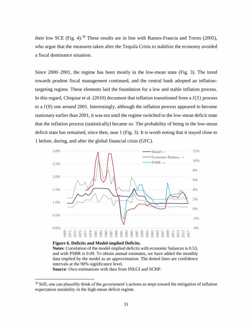
their low SCE (Fig. 4).39 These results are in line with Ramos-Francia and Torres (2005),
who argue that the measures taken after the Tequila Crisis to stabilize the economy avoided
a fiscal dominance situation.
Since 2000–2001, the regime has been mostly in the low-mean state (Fig. 3). The trend
towards prudent fiscal management continued, and the central bank adopted an inflation-
targeting regime. These elements laid the foundation for a low and stable inflation process.
In this regard, Chiquiar et al. (2010) document that inflation transitioned from a 𝐼(1) process
to a 𝐼(0) one around 2001. Interestingly, although the inflation process appeared to become
stationary earlier than 2001, it was not until the regime switched to the low-mean deficit state
that the inflation process (statistically) became so. The probability of being in the low-mean
deficit state has remained, since then, near 1 (Fig. 3). It is worth noting that it stayed close to
1 before, during, and after the global financial crisis (GFC).
Figure 6. Deficits and Model-implied Deficits.
Notes: Correlation of the model-implied deficits with economic balances is 0.53,
and with PSBR is 0.09. To obtain annual estimates, we have added the monthly
data implied by the model as an approximation. The dotted lines are confidence
intervals at the 90% significance level.
Source: Own estimations with data from INEGI and SCHP.
39 Still, one can plausibly think of the government’s actions as steps toward the mitigation of inflation
expectation instability in the high-mean deficit regime.
-4%
-2%
0%
2%
4%
6%
8%
10%
12%
0.0%
0.5%
1.0%
1.5%
2.0%
2.5%
3.0%
196
9
197
1
197
3
197
5
197
7
197
9
198
1
198
3
198
5
198
7
198
9
199
1
199
3
199
5
199
7
199
9
200
1
200
3
200
5
200
7
200
9
201
1
201
3
201
5
201
7
Model ←
Economic Balance →
PSBR →

32
8. Final Remarks
Historically, Latin American economies have partially financed their fiscal deficits through
seigniorage. One common characteristic of economies in the region is that they have allowed
the inflationary tax to have an active role. Mexico has not been the exception in this regard.
In the past, it used several times the inflationary tax to finance its fiscal deficit; i.e., to close
the gap in the government’s intertemporal budget constraints.
As a consequence, the country had to bear eventually substantial costs in terms of inflation,
fiscal imbalances, and indebtedness and, in some cases, economic crises. In response, the
government confronted the associated challenges implementing several adjustment
programs, many of which proved initially insufficient. Several factors were crucial for these
programs to succeed eventually. For example, under the presence of debt overhang, the
renegotiation of the external debt proved pivotal. In the context of the model, such factors
made the transition from the high-mean fiscal deficit regime to the medium- and low-mean
fiscal deficit regimes feasible, making fundamental reforms possible in the model.
The model captures the dynamics of inflation, inflation expectations, and seigniorage-
financed fiscal deficits in a parsimonious way (e.g., see Sargent and Wallace, 1981). In effect,
the interaction of the demand for money, the intertemporal government budget constraint,
and the distribution of the fiscal deficits does a good job of characterizing the macroeconomic
variables’ dynamics. The regimes that are part of the distribution of fiscal deficits enable a
better characterization of such dynamics.
It is worth reemphasizing that it has been several years since there was a favourable regime
change in the stability of inflation and its expectations. From several perspectives, such a
result is naturally quite important. Even so, we should not forget the hard-earned lessons. All
in all, bearing the interdependence of monetary and fiscal policies in mind and sparing no
efforts in maintaining discipline in both are key elements for the macroeconomic stability of
the economy.

33
References
[1.] Bruno, M. (1989). “Econometrics and the Design of Economic Reform”.
Econometrica, Vol. 57, No. 2, pp. 275–306.
[2.] Bruno, M., and Fischer, S. (1990). “Seigniorage, operating rules, and the high
inflation trap”. The Quarterly Journal of Economics, Vol. 105, No. 2, pp. 353–374.
[3.] Buiter, W. H. (1987). “Borrowing to defend the exchange rate and the timing and
magnitude of speculative attacks”. Journal of International Economics. Vol. 23, No.
3–4, November, pp. 221–239.
[4.] Buiter, W. H. (2001). “The Fiscal Theory of the Price Level: A Critique*”. Working
Paper, European Bank for Reconstruction and Development.
[5.] Cagan, P. (1956). “The monetary dynamics of hyperinflation”, in M. Friedman
(editor), Studies in the Quantity Theory of Money. University of Chicago Press.
[6.] Chiquiar, D., A. E. Noriega, and M. Ramos-Francia (2010). “A time-series
approach to test a change in inflation persistence: the Mexican experience”. Applied
Economics, Vol. 42, No. 24, pp. 3067–3075.
[7.] Gil-Díaz, F., and A. Carstens (1996a). “Some Hypotheses Related to the Mexican
1994–95 Crisis” Banco de México. Working Papers.
[8.] Gil-Díaz, F., and A. Carstens (1996b). “One year of solitude: Some pilgrim tales
about Mexico's 1994–1995 crisis”. The American Economic Review, Vol. 86, No. 2,
164–169.
[9.] IMF (2001). Silent Revolution: The IMF 1979-1989, October 1, 2001, Chapter 7 - The
Mexican Crisis: No Mountain Too High?
[10.] Kushner, H. J. and G. G. Yin. (1997). “Stochastic Approximation Algorithms and
Applications”. New York: Springer-Verlag.
[11.] Leeper, E. M. (1991). “Equilibria under ‘Active’ and ‘Passive’ Monetary and Fiscal
Policies”. Journal of Monetary Economics, Vol. 27, No. 1, pp. 129−147.
[12.] Lopez-Martin, B., A. Ramírez de Aguilar, and D. Sámano (2018). “Fiscal Policy
and Inflation: Understanding the Role of Expectations in Mexico” Banco de México.
Working Paper No. 2018-18.

34
[13.] Meza, F. (2018). “Mexico from the 1960s to the 21st Century: From Fiscal Dominance
to Debt Crisis to Low Inflation”. Manuscript.
[14.] Musacchio, A. (2012). “Mexico’s financial crisis of 1994–1995”. Harvard Business
School. Working Paper 12-101.
[15.] Ortiz, G. (1991). “Mexico Beyond the Debt Crisis: Toward Sustainable Growth with
Price Stability”, in M. Bruno, S. Fischer, E. Helpman and N. Liviatan (editors), Lessons
from Economic Stabilization and its Aftermath, MIT Press.
[16.] Ramos-Francia, M. (1993). “Essays on Money and Inflation in Mexico”, Ph.D.
Dissertation, Yale University.
[17.] Ramos-Francia, M. and A. Torres (2005). “Reducing Inflation through Inflation
Targeting: The Mexican Experience”. pp. 1–29, in R. J. Langhammer and L. Vinhas
de Souza (editors), “Monetary Policy and Macroeconomic Stabilization in Latin
America”, Kiel 5 Institute for World Economics, Springer-Verlag.
[18.] Sachs, J.D. (1989). “New Approaches to the Latin American Debt Crisis”. Essays in
International Finance No. 157. July.
[19.] Sanginés, A. (1989). “Managing Mexico's External Debt: The Contribution of Debt
Reduction Schemes”. The World Bank Internal Discussion Paper.
[20.] Sargent, T., and N. Wallace (1981). “Some unpleasant monetarist arithmetic”.
Federal Reserve Bank of Minneapolis Quarterly Review, Fall, pp. 1–17.
[21.] Sargent T., N. Williams, and T. Zha (2009). “The Conquest of South American
Inflation”. Journal of Political Economy, Vol. 117, No. 2, pp. 211–256.
[22.] SHCP (2014). “Public Sector Borrowing Requirements and their Historical Balance,
Methodology”. URL: www.apartados.hacienda.gob.mx
[23.] Sidaoui, J. J. (2000). “Macroeconomic Aspects of the Management of External Debt
and Liquidity” in BIS (2000) “Managing Foreign Debt and Liquidity Risks”, BIS
Policy Papers No. 8.
[24.] Sims, C. A., D. F. Waggoner, and T. Zha (2008). “Methods for inference in large
multiple-equation Markov-switching models”. Journal of Econometrics, Vol. 146, No.
2, pp. 255–274.

35
[25.] van Wijnbergen, S., M. King, and R. Portes (1991). “Mexico and the Brady Plan”.
Economic Policy, Vol. 6, No. 12 (Apr.), pp. 13–56.
[26.] Whitt, J. A. (1996). “The Mexican Peso Crisis” Federal Reserve Bank of Atlanta,
Economic Review, Vol. 81, No. 1.

36
Appendices
Appendix A. The Public Sector Borrowing Requirements
Based on (SHCP, 2014), we have the following descriptions. The Public Sector Borrowing
Requirements (PSBR, or RFSP for its acronym in Spanish) is the broadest definition of the
government deficit. It adds the following six elements to the economic balance. First, it
includes the financial requirements of the Infrastructure Investment Projects with Deferred
Public Expenses Registry (PIDIREGAS, in Spanish). PIDIREGAS commonly refers to
public works projects financed by the private sector and executed by a private company. The
government defers its registry, based on the General Public Debt Law. PSBR registers the
resource requirements as the public work progresses, and the respective entity amortizes it.
In contrast, the economic balance registers it once the contractor delivers the public work in
question.
Second, it considers the financial requirements of the Bank Savings Protection Institute
(IPAB, in Spanish). The total financial requirements of IPAB are not included in the
economic balance based on the Bank Savings Protection Law (see Article 47). The economic
balance only includes the fiscal support covering the real component of the financial cost that
the referred institute faces.
Third, the included budget registry adjustments mainly refer to the following: a) the
inflationary component of index-linked debt; b) the possible revenue due to debt buybacks;
c) the income due to debt issuance above or below par (note that PSBR measures public debt
based on its issuance value); and d) the Social Security actuarial reserves (i.e., Mexican
Social Security Institute, and the Mexican Civil Service Social Security and Services
Institute, IMSS and ISSTE, for their acronyms in Spanish).
Fourth, it encompasses the financial requirements of the National Infrastructure Fund
(FONADIN, in Spanish) and those derived from the Road Rescue Program and new
resources allocated to infrastructure development not financed by budget expenses. Fifth, it

37
considers the debtors program, which includes the discounted payments and investments
units (i.e., UDIs, in Spanish) restructuring programs.
Lastly, it adds the expected profits and losses of development banks and public
funds regulated and supervised by the National Banking and Securities Commission
(CNBV, for its name in Spanish), but does not consider their financial intermediation
deficit. The PSBR does not include nonrecurring revenues, including revenues from
privatizations, asset recovery from trusts and funds, and excess profits received from
public entities. Its new methodology considers activities of the private sector when it is
acting on behalf of the federal government or its entities, adjusted for the revenue
obtained from the net sales of financial assets and the net acquisition of liabilities different
from public debt.
Appendix B. Inflation We present the inflation time series along with the model-implied inflation.
Figure B1. Inflation (Data) and Inflation (Model). Notes: The correlation coefficient between the model inflation and the data is 0.87. Annualized monthly inflations. Source: Own estimations with data from INEGI.
-50
0
50
100
150
200
250
19
68
19
70
19
72
19
74
19
76
19
78
19
80
19
82
19
84
19
86
19
88
19
90
19
92
19
94
19
96
19
98
20
00
20
02
20
04
20
06
20
08
20
10
20
12
20
14
20
16
20
18
Inflation (Data) Inflation (Model)