Inferring the topology of a non-linear sparse gene regulatorynetwork using fully Bayesian spline regression

Edward R. Morrissey, Miguel A. Juárez�, Nigel J. BurroughsSystems Biology Centre

University of Warwick, UK

Katherine J. DenbySystems Biology Centre and HRI

University of Warwick, UK

Abstract

We propose a semi-parametric Bayesian model, based on penalised splines, for the recovery of the topology ofan interaction network from longitudinal data. Our motivation is inference of gene regulatory networks fromlow resolution microarray time series (10 � 50 time points). Parenthood relations are mapped by augmentingthe model with kinship indicators and providing these with either an overall or gene-wise hierarchical struc-ture. Appropriate specification of the prior is crucial to control the flexibility of the splines, especially undercircumstances of scarce data; thus we provide an informative, proper prior and analyse sensitivity. The posterioris analytically intractable and numerical methods are needed. A Metropolis-within-Gibbs sampler is proposed,with a novel Metropolis-Hastings step for sampling the topology and the spline coefficients simultaneously. Wealso construct a linear model for comparison purposes. Model fit is illustrated using synthetic data drawn fromODE models and and gene expression from an experimental data set of the Arabidopsis thaliana circadian rhythm.

Keywords: Circadian clock, Gibbs variable selection, Markov process prior, non-linear gene regulatory net-works, P -Splines regression, time course gene expression data.

1 INTRODUCTION

Modern DNA sequencing technology has enabled the genome of many organisms to be determined ranging fromsmall unicellular genomes such as those of bacteria and yeast, to complex large genomes, such as for humans (seee.g. www.ncbi.nlm.nih.gov and www.ebi.ac.uk). Knowledge of the genome is fundamental, given that gene/proteininteractions are responsible for cell (and tissue) function. A key component of this interaction process is generegulation, specifically the degree to which a gene is expressed, when, and for what duration. Gene expressionis the conversion of the (sequence) information in the gene into messenger RNA (mRNA) by a process termedtranscription and then to a functional protein by translation, resulting in the phenotypic expression of the gene.Gene expression, quantified as the amount of mRNA, can be measured by a number of technologies, the mostcommon being microarrays although sequencing (RNA-seq) is becoming increasingly popular. Despite knowledgeof the genome sequence, a key issue is identifying what events and which proteins control expression of individualgenes. This information cannot presently be determined from the genome sequence alone.

Gene regulation is a complex process, the actual regulators being proteins, or complexes of proteins that bindjust upstream of the gene and regulate the rate of that gene’s transcription. Various processes can regulate theamount of active protein at a given time, regulation that depends on the nature of the organism and the specificgene. Specifically, regulation can occur through the rate of transcription, modification of the mRNA (e.g. splicing),

�Corresponding author: Miguel A. Juárez, University of Warwick, Systems Biology Centre, Coventry House, CV4 7AL, Coventry,UK. Email: m.a.juarez@warwick.ac.uk

1

2 1. INTRODUCTION

decay rate of the mRNA, the rate of translation, the folding efficiency of the protein, the decay rate of the proteinand through a number post-translational modifications, such as phosphorylation, that affect the activity of theprotein, i.e. its capability of carrying out specific functions. Regulation of a gene’s transcription rate is then anintegration of all these processes applied to its regulators, coupled with the kinetics and combinatorics of thoseregulators in binding to the gene’s regulatory sequences. In this manner, by mapping gene regulation back to genes,we obtain a vast interconnecting gene regulatory network (grn). Many biotechnical and medical problems haveat their core a grn, for instance, the immune system (Gilchrist et al., 2006), the mode of action of antibiotics(Kohanski et al., 2008) and crop yield (Yin et al., 2004).

The complexity of gene regulation, and the complex association of steps from transcription through to func-tional protein make inference of gene-gene regulatory interactions from mRNA data difficult; essentially we onlyhave transcriptional changes, both in the regulator and regulatee from which to infer regulatory interactions. Thecatalogue of post-transcriptional changes mentioned above are extremely difficult to measure on a global basis, anda partial analysis can only be performed on a small number of select proteins. From a modelling standpoint, agrn can be thought of as a directed graph, with the nodes representing genes and the edges regulatory relationships(Gardner et al., 2000; Hache et al., 2009; Hartemik, 2005; Ronen et al., 2002). One of the main obstacles when re-trieving the interaction structure, i.e. the topology, of a grn is the combinatorial growth of the network topologyspace with respect to the number of genes considered. Further, it has been proven that finding the maximum aposteriori (MAP) network is an NP-hard problem (Shimony, 1994). Thus, several approximations to estimating thetopology of the network have been proposed, for instance, Chen and Zheng (2009), Ahn et al. (2009) and Schäferand Strimmer (2005) use (partial) correlations as an association measure and select the significant edges by con-trolling for the false discovery rate; while Faith et al. (2007) employs a variant of the Kullback-Liebler divergence asa measure of association and selects the edges by testing the estimated divergences against a background distributionof the scores related to the relevant node. Reviews are provided i.a. Bansal et al. (2007), Jaffrezic and Tosser-Klopp(2009) and Yu et al. (2004).

In any living organism, the cell has to cope with a plethora of environmental conditions, and thus has readilyavailable adaptation mechanisms. For any specific process, typically only a small fraction of the genome is active,e.g. the SOS pathway in Escherichia coli (Courcelle et al., 2001). This modularity and specialisation gives the regulat-ory network a key characteristic that is vital in inference, essentially the network is sparse with considerably fewerthan the G.G � 1/ possible interactions on G genes.

Using time series data, our main objective is inference of grns. In particular, we are interested in inferring thegene regulatory kinships for a given process. When stated in a graphical manner such relationships are representedas edges and the genes as nodes; these edges can be directed or not, and feedback loops and cliques may or may notbe allowed. One very well known example of such graphs is a directed acyclic graph, characterised by directed edgesand a tree structure (Bang-Jensen and Gutin, 2009; Jensen and Nielsen, 2007). From a Bayesian perspective, whichwill be followed in this paper, these are usually estimated using Bayesian Networks (Cowell et al., 1999; Lauritzen,1996).

Bayesian networks (BN) have been used previously in gene network determination (Friedman, 2004; Friedmanet al., 2000; Hongqiang et al., 2005). However, it is well known that biological processes have feedback loops andthus the validity of BNs is questionable when modelling such systems. Dynamic Bayesian networks (dbn) havebeen proposed for modelling time course (longitudinal) gene expression data (Cao and Zhao, 2008; Kim et al., 2003;Murphy and Mian, 1999; Perrin et al., 2003; Zou and Conzen, 2005). These can be thought of as “unfolding” a BNfor every time point and when folding back the network self-regulation and cliques may be obtained. Formally,a dbn is characterised by a set of conditional relations, p

�ytC1

j y t�. In the case of a regression based dbn these

relations can be written as ytC1i D fi

�y t

�C "tC1

i , where yti is the measurement of gene i D 1; : : : ; G, at time

t D 1; : : : ; T , y t D˚yt

1; yt2; : : : ; yt

G

and "t

i is an idiosyncratic error term. The functional forms of the interactions,

1. INTRODUCTION 3

fi .�/, are usually unknown. Whether or not @fi

�y t

�=@yt

j � 0 defines the topology of the network. The interactiontopology is key in grn, as it determines the causal relations in the gene regulatory dynamics for a given biologicalprocess. In turn, the estimated network can be used to propose new experiments —e.g. gene knockouts— to furtherunderstand said process. This programme of experimenting-modelling-hypothesising-experimenting is at the heartof Systems Biology.

Irrespective of the actual form of fi .�/, dbn are typically heavily parameterised. If we consider a network of G

genes, we need to estimate G2 interactions (edges), in addition to any other parameters involved in the model. Acommon approach is to assume the simplest form of interaction, specifically a linear form. In biochemical reactionmodelling, regulatory relations are frequently modelled as systems of ordinary differential equations (ODEs), withmonotonic functional interactions, and thus linearity is justified as a first order Taylor expansion (di Bernardo et al.,2005; Bonneau et al., 2006; Gardner et al., 2003). Frequently, however, the linear assumption does not hold in prac-tice. This may be due to a large spacing between measurements, thus rendering the linear approximation invalid.Another reason is that some of the interactions are indeed highly non-linear, given the extensive set of processesinvolved in protein expression, and the fact that regulators often work together, either synergistically, for instancethrough binding to form a larger complex, or antagonistically, for instance competing for binding to overlappingregulatory regions on the genome. Further, even when linearity is appropriate, its range may be limited throughsaturation effects (e.g. unlimited amounts of mRNA cannot be produced), or there may be a minimum amount ofany given regulator required in order for a reaction to take place or to be detectable by the measurement device.Linear specifications of the network interactions are incapable of capturing such effects. Specific forms of nonlin-earity for the interactions can be assigned (power, exponential, Michaelis-Menten, etc.); however, misspecificationof the actual shape may yield a spurious estimate of the network topology.

A flexible way of including unknown non-linearities, and thus avoiding model selection issues, is to use a semi-parametric specification by letting the interactions be described by spline functions. There is a vast literature onspline curve smoothing (Denison et al., 1998; Dierckx, 1993; Fan and Gijbels, 1996; Wahba, 1990; Wand and Jones,1995) and spline regression (Biller, 2000; Green and Silverman, 1994; Marx and Eilers, 1998; Wu and Zhang, 2006).Within grns, smoothing of discretely observed gene expression time series with splines to aid in the retrieval ofgrns has been advanced by e.g. Gustafsson et al. (2005), Opgen-Rhein and Strimmer (2006), Toyoshiba et al. (2004),while Kim et al. (2004) use spline regression for grn inference. One fundamental problem when using splineregression is knot selection which greatly influences the curve fitting. One efficient solution is to select a few wellplaced knots for a given spline degree. This implies determining both the optimal number and position of theknots, which is typically addressed by means of a trans-dimensional mcmc scheme (Denison et al., 2002; DiMatteoet al., 2001; Ferreira et al., 2008) or by cross-validation (Friedman, 1991; Ruppert, 2002). The efficiency gained in themodelling may be offset by mixing problems in the sampler, due mainly to the vast space that must be explored andthe associated computational problems, or by the unwieldy amount of comparisons required for cross-validation.

Our approach avoids such issues by relying on P -splines (Brezger and Lang, 2008; Eilers and Marx, 1996; Langand Brezger, 2004), which are characterised by specifying a rather large number of evenly spaced knots. Then, inorder to avoid over-fitting and also to control for the effective number of parameters to be estimated, a penaltythat shrinks the spline coefficients towards the origin is specified. Such a penalty depends crucially on a so-calledsmoothness parameter. Imoto et al. (2002) propose a semi-parametric P -spline regression model for grn retrieval,optimising the smoothness parameter using a modified BIC and then performing a greedy search on the network to-pology space. Imoto and Konishi (2003) discuss the use of a modified AIC for optimising the smoothing parameterin a similar context. In this paper, we propose a fully Bayesian set up for dealing with this smoothness parameterand discuss the implications of alternative prior specifications for this key model component.

Nonlinear interaction models entail a larger number of parameters compared to the linear case. Given theunderdetermined nature of network inference typically presented by microarray data on small time series data

4 2. THE MODEL

sets, this increase in complexity needs careful handling. Our solution is to impose sparsity on the network, as isbiologically justified, through use of a spike-and-slab prior. We augment our model with kinship indicator variables,and determine the network topology by carrying out a Gibbs variable selection procedure. This leads to a dramaticimprovement in power, and thus the availability of information on many of the inferred links. Through carefulconstruction of a prior to control spline complexity, we achieve a balance between limited information and modelcomplexity.

Given the significant interest in estimating grns, there is a vast growing literature on this problem. Most ofthe approaches dealing with longitudinal grns are based on autoregressive models, and given that the number oftime measurements is rather small, an AR(1) specification is pervasive. For instance, Opgen-Rhein and Strimmer(2007) uses a linear AR(1) specification for the regulatory interactions and shrink the AR coefficients using a James-Stein type estimator. Network retrieval is performed by identifying the significant partial correlations by meansof a local false discovery rate. Lèbre (2009) proceeds in a very similar fashion, from the same linear setup partialregression coefficients are tested to reduce the space of possible links. The final network is obtained by performinga further t -test on the estimated regression coefficients of the restricted network. In contrast, our splines modelis semi-parametric, allowing for non-linear interactions within a context of simultaneous topology (edge) selectionachieved through use of Gibbs variable selection.

The model proposed is presented in Section 2, where we also discuss the prior specification. Given that it iscommon to specify an improper prior for this kind of model, we provide sufficient conditions for posterior propri-ety, and also provide an alternative, proper prior. The resulting posterior distribution is intractable analytically andin Section 3 we provide an mcmc scheme for sampling the posterior with a novel Metropolis-Hastings step whichimproves mixing and convergence of the chain. Section 4 illustrates the application of our model to three examples,where we reconstruct the corresponding networks and assess their accuracy. We also provide some guidelines forcalibrating the prior. Conclusions and possible extensions are given in Section 5. Data sets and Matlab code used inthe paper are available upon request.

2 THE MODEL

Let ytg denote the gene expression measurement of gene g D 1; : : : ; G, at time t D 1; : : : ; T . We propose to model

it asyt

g D �tg C "t

g ; (1)

where �tg is the predictor and "t

g is an idiosyncratic error term, centred at zero. We assume that �tg is determ-

ined by some unknown subset of the genes at the previous time point, and that the error terms are Gaussian andindependent for all genes and time points. Thus, we can write (1) as

ytg D �g

�y t�1

I �g

�C "t

g ; "tg � N

�"t

g j 0; �g

�ind : (2)

with y t�1 D˚yt�1

1 ; : : : ; yt�1G

, �g a set of parameters indexing �g.�I �/ and ��1

g D Var."tg/.

In order to accommodate nonlinearities, we use a flexible, non-parametric setting for the mean level, based onB -splines (Eilers and Marx, 1996). Thus,

�tg D fg1

�yt�1

1

�C fg2

�yt�1

2

�C � � � C fgG

�yt�1

G

�C �g ; (3)

where

fgi .yi/ D

MXkD1

ˇg

ikBik.yi/ :

2.1. THE PRIOR 5

Here, �g is a gene-specific constant term, M D r C l is the number of spline basis functions, Bik.yi /, of degree l ,defined over the set, �i D f�i1; : : : ; �irg, of r evenly spaced knots,

min fyig D �i1 < �i2 < � � � < �ir D max fyig :

The basis functions Bik are nonzero only in a domain spanned by 2 C l (adjacent) knots. By defining the splinedesign row vectors X t

j 2 RM , such that X tj .k/ D Bjk

�yt

j

�, we can rewrite the predictor as

�tg D X t�1

1 ˇ1g C � � � C X t�1G ˇGg C �g

with jg D

nˇ

gj1; : : : ; ˇ

gjM

o2 RM a column vector of coefficients for j D 1; : : : ; G. If k jgk � 0, there is

negligible influence of gene j on gene g, and thus deem the link from j to g as off. If the link is on, then we saythat j is a parent of g.

Stacking the bases and the coefficients into X t D˚X t

1; : : : ; X tG

2 RMG and ˇg D fˇ1g ; : : : ; ˇGgg 2 RMG ,

respectively, we can express the model as ytC1g D �g C X tˇg C "t

g and after further stacking the equations overtime we have,

yg D �g C X ˇg C "g ; g D 1; : : : ; G ; (4)

where �g D �g�0T , with �T a row vector of ones of size T and X D

˚X1; X2; : : : ; XT

0 a bases matrix of sizeŒT � MG�. This model is unidentifiable given that every potential parent spline contributes with its own constantterm. To correct for this, we add the identifiability restriction �T � ŒX ˇg � D 0. We describe its implementationwithin the sampling scheme in Section 3.

As it stands, (4) would require at least M � G data points per gene to be estimated. If the number of timemeasurements is relatively small, one would need to select a rather small number of knots, thus effectively reducingthe capacity of the splines to capture non-linearities. Furthermore, in genetics applications data are typically ob-tained from high throughput methods, such as microarrays, providing measurements from hundreds to thousandsof genes at every time point, while the actual number of time measurements, T , is generally not more than a fewdozen. It is then necessary to introduce some degree of sparseness into the link structure, i.e. restrict the numberof potential parents, in order to carry out any estimation. Also, it is well known that in any given biological pro-cess, typically only a handful of genes are responsible for gene activity, and thence this restriction arises naturally.We accommodate this idea by performing a Gibbs variable selection as in Smith and Kohn (1996). The model isaugmented with the indicators jg , such that

zjg D jg � jg where jg D

˚1 the link is on

0 the link is off:

and substituting these new coefficients into the model. From a Bayesian perspective this can also be thought of asa spike-and-slab prior specification (Ishwaran and Rao, 2005; Mitchell and Beauchamp, 1988) on the spline coeffi-cients. The practical advantage of augmenting with the indicators, jg , is that it allows us to make inference aboutthe network topology, now parameterised by the connectivity matrix, � D f jgg.

2.1 THE PRIOR

Here we complete the specification of our Bayesian model by formalising the prior specification. Conditionallyconjugate priors are used where suitable, which simplifies the sampling algorithm.

We take particular care when specifying a shrinkage or penalty prior for the spline coefficients, as this determ-ines the smoothness of the functional form fitted. It will become apparent that in the cases where the data is scarce,

6 2.1. THE PRIOR

this part of the prior is crucial and therefore we discuss some alternatives and perform associated sensitivity ana-lyses. We assume that the data have been standardised (zero mean and unit variance for each gene), so we need notintroduce gene specific scalings in the prior.

Precisions We use conjugate, iid gamma priors, Ga.�g j a�; b�/, on the gene precisions, � = f�1; : : : ; �Gg,

 .�/ D

GYgD1

ba�

�

� Œa���a��1

g exp Œ�b� �g � : (5)

Constant term An independent Gaussian prior, N.� j 0; ��I/, for the gene-specific constant, � = f�1; : : : ; �Gg

 .�/ D

� ��

2 �

�G=2

exph�

��

2�0 �

i: (6)

Network structure We provide two alternatives for modelling the network topology. The first is to define theoverall network connectivity, �, as P

� jg D 1

�D � and complement it with a Beta prior, Be.� j a�; b�/. The

full specification is then,

 . jg j �/ D � jg .1 � �/1� jg ; g; j D 1; : : : ; G ; (7)

 .�/ D ŒB.a�; b�/��1

�a��1.1 � �/b��1 0 < � < 1 : (8)

It is well known that grns often present hub-like structures, where a handful of genes control the regulationprocess almost completely and with the rest of genes having very few children, if any (see e.g. Seo et al., 2009,and references therein). One can capture such features by allowing for parent-wise connectivity, P Œ jg D 1� D

�j , and complementing it with independent priors, i.e.

 . jg j �j/ D � jg

j .1 � �j/1� jg ; g D 1; : : : ; G ; (9)

 .�j/ D ŒB.a�; b�/��1

�a��1

j .1 � �j/b��1 j D 1; : : : ; G : (10)

The hyperparameters fa�; b�g, convey our prior knowledge about the connectivity of the network and canbe set accordingly. For general purposes, we recommend setting both equal to 1=2, as this is the referenceprior for a Bernoulli experiment (Bernardo and Smith, 1994). If biological knowledge of the process demandsit, it is straightforward to fix any link to be deterministically on (off) by setting rl D 1.0/, modifying theprior accordingly.

Spline Coefficients We use the prior on the coefficients jg to shrink them towards the origin. One option is topenalise using a Gaussian process prior as in Speckman and Sun (2003). However, we follow Eilers and Marx(1996), specifying a second order Markov process prior

 . jg j �jg/ D N. jg j 0; �jg K/ : (11)

Where �jg are the smoothness parameters addressed below. The structure of the covariance matrix, K, isconstructed from the second order differences between adjacent coefficients, i.e., ˇk D 2 ˇk�1 � ˇk�2,omitting link identifiers for simplicity. Thus,

K.M; M � 2/ D 1 ; K.M � 2; M � 1/ D �4 ; K.M; M/ D 1 ;

K.M; M � 1/ D �2 ; K.M � 1; M � 1/ D 5 I

2.1. THE PRIOR 7

and for all i; j 2 f3; : : : M � 2g,

K Œi; j � D

˚0 ji � j j > 2

�4 ji � j j D 1

1 ji � j j D 2

6 ji � j j D 0

:

The two remaining coefficients are given a constant (improper) prior  .ˇ1; ˇ2/ / 1.

Smoothness parameters In the case of small data sets the specification of the smoothness parameters, �jg , becomescrucial as these largely determine the fitting of the spline to the data. In the limit, when �jg ! 0 an interpol-ating spline is fitted, while as �jg ! 1 a straight line is rendered. Various alternatives have been proposed fordealing with the smoothing parameters (Belitz and Lang, 2008; Kohn et al., 1991; Speckman and Sun, 2003;Wand, 1999). Following Fahrmeir and Lang (2001) and Lang and Brezger (2004), we perform a full Bayesiananalysis and specify priors for the smoothing parameters.

The conditionally conjugate prior is the product of independent gamma distributions, Ga.� j a� ; b�/. Thisspecification concentrates mass around a�=b� and has a relatively large right tail for small values of b� . It iscommon to find in the literature a� D b� and set to quite small values, e.g. 0.001. This indeed is quite flatover a large range of � , but has a mode at zero effectively giving relative importance to rougher curves andthus favouring over-fitting when the data is only weakly informative. On the other hand, if mass is carriedtowards larger values of � —thus favouring smoother curves— the gamma distribution tails off quite quicklyto the left and experiences difficulties capturing non-linearities, (see e.g. Jullion and Lambert, 2007).

In order to obtain a more flexible prior specification, while retaining the conditional conjugacy, we also trieda gamma scale mixture of gammas. The resulting gamma-gamma distribution (Bernardo and Smith, 1994,p. 120; Zellner, 1971, p. 376), can achieve a larger spread than the gamma and also has a heavier right tail.It may also not have any moments for certain parameter values. Despite these desirable characteristics, wefound that the heavy right tail of this prior, combined with the flatness of the likelihood in regions where �

is very large can lead to identifiability issues. This can be understood since there exists a threshold value, �?,for which the fit of the spline is practically linear and thus indistinguishable for any � > �?.

This lead us to propose an inverted Pareto prior, Ip.� j a� ; b�/:

 .�jg j a� ; b�/ Da�

b�

��jg

b�

�a� �1

; �jg � b� ; a� > 0 : (12)

We restrict a� � 1, to prevent concentration of mass near the origin. Setting a� D 1 is tantamount to puttinga uniform prior on .0; b�/. If a� > 1, the prior behaves as a power function and gathers mass closer to b� as a�

grows, thus favouring smoother curves. Values of a� > 3 allocate too much mass close to b� and thus are notadvisable, unless there is prior evidence for high levels of linearity. The cut-off value b� can be interpretedas that level of � after which the likelihood is numerically invariant, i.e. the fitted curve is practically linear.Determining the value of b� could be done, for instance, by cross-validation if feasible; otherwise, a sensitivityanalysis should be carried out.

The resulting conditional posterior is amenable to a Gibbs step, requiring sampling from a truncated distri-bution. Details are given in Section 3.

8 3. IMPLEMENTATION

2.1.1 POSTERIOR PROPRIETY

Fahrmeir and Kneib (2009) discuss conditions for posterior propriety using this covariance structure and differentalternatives for the smoothing parameters within the context of structured additive models. We provide a resultjustifying an extension of this prior for grn inference. The proof is standard and therefore omitted.

Theorem 1.Consider the longitudinal data set Y D

˚yt

g

, consisting of g D 1; : : : ; G genes measured at times t D 1; : : : ; T ,

modelled as (4) and with prior given by (5)–(12). Denote by G? the number of parents of gene g. Let

Kg D blkdiag Œ�1gK; �2gK; : : : ; �G?gK� and g D X 0gXg C Kg :

Where Xg is the design submatrix conformable to G?. Then, the posterior distribution of fˇ1; : : : ; ˇG ; �g is proper ifg is positive definite for every g and M � G? < T .

Given that in most of our applications we will only have a limited number of time measurements compared tothe number of genes, this leads to an improper posterior if the prior was not proper, since the number of parentsfor any given gene only needs to exceed T=M . To construct a proper prior we supply (11) with an independentspecification for the first two coefficients,

 .ˇ1; ˇ2/ D N.ˇ1 j 0; k1/ N.ˇ2 j 0; k2/ : (13)

Including these into the covariance structure we have,

K.1; 1/ D .1 C k1=�/ ; K.1; 2/ D �2 ; K.1; 3/ D 1 ; K.2; 2/ D .5 C k2=�/ ; K.2; 3/ D 1 :

for the appropriate smoothness parameter, � . To approximate the behaviour of the improper prior, we could letk1; k2 ! 0. In situations where the data is scarce, we do not recommend this, as it will affect the stability of theposterior (Lambert et al., 2005; Sun and Speckman, 2008). In our applications, we set k1 D k2 D �0.

3 IMPLEMENTATION

3.1 P -SPLINES MODEL ALGORITHM

Combining the likelihood (4) with the prior (5)–(13) and letting � denote all the model parameters we obtain,

 .� j X ; Y/ /

�Yg

NT

�yg j �g C X z

g ; �gIT

�� �Yg

 .ˇg j �g/ .�g/ .�g/ .�g/ . g j �g/ .�g/�

;

where IT is the identity matrix of size T , g D f 1g ; : : : ; Ggg and �g D f�1g ; : : : ; �Ggg. As there is no closedform expression for the posterior numerical methods are needed. We propose a Metropolis-within-Gibbs schemewhich is drafted below.

Precisions The full conditional of �g , g D 1; : : : ; G is given by

 .�g j —/ / �T=2Ca��1g exp

���g

�b� C

1

2

�yg � �g � X z

g

�0�yg � �g � X z

g

���which is the kernel of a gamma distribution.

3.1. P -SPLINES MODEL ALGORITHM 9

Constant term �g is conditionally Gaussian, with mean and precision

mg Dxyg � xX z

g

�g C ��=Tand � 0

� D �� C T �g ;

respectively, where xyg D T �1P

t ytg and xX D T �1

Pt X .

Connectivity If (9)–(10) is used, the full conditionals for the gene-wise connectivities, �g , are obtained as

 .�g j —/ / �SgCa��1g .1 � �g/GCb��Sg�1 with Sg D

GXi

gi for g D 1; : : : ; G ;

and are sampled from a Be.�g j Sg C a�; G C b� � Sg/.

If (7)–(8) is used instead, the overall connectivity, �, is sampled from a Be�� j S C a�; G2

C b� � S�, with

S DPG

gD1 Sg .

Smoothness parameters When the corresponding link is on, the full conditional is given by

 .�jg j —/ / �.M � 2/=2Ca� �1

jg exp���jg

1

2z0jgK z

jg

�; 0 < �jg < b�

and can be sampled from a truncated gamma distribution (Damien and Walker, 2001; Gentle, 2003) withparameters

n.M � 2/=2 C a� ; z0

jgK zjg=2

o. An observation is drawn from the prior when the link is off.

Spline Coefficients and link probabilities The update of the spline coefficients and indicator variables is per-formed as a block. Specifically, the update of a given indicator variable jg and all the coefficients of theregression for gene g, ˇg , are performed simultaneously. In practice, as the regression is sparse, only a fewlinks are actually present drastically reducing this computation. At every iteration, the individual link indic-ator jg is turned on (off) if it is off(on) and the associated coefficient, ˇg 2 RMG , for present links (on) isproposed from the joint conditional, schematically:

W 0 ! 1 and ˇ W ˇa! ˇb

with acceptance probability

˛ D min

( 

�zb

� 

�za

� q.ˇa j a/q. a/

q.ˇb j b/q. b/; 1

);

where the subscripts have been omitted for clarity. is proposed symmetrically, thus q. a/=q. b/ D 1. Forq.ˇ j / we use the proposal

q.ˇ j —/ D N.�ˇ; ˙ˇ/

with

˙ˇ D��gX 0

gXg C �g

�and �ˇ D �g.yg � �g/Xg˙�1

ˇ ;

where �g is the block diagonal penalty (precision) matrix, calculated by multiplying each block in Kg timesthe corresponding �jg . Note that, as only the coefficients with non zero indicator variable are updated, Xg ,

10 3.2. A LINEAR MODEL

yg and �g are adjusted to only include the appropriate elements. Substituting this in the Hastings ratio gives

�

1 � ��0�

.M�2/=2jg

exp�

1

2�b

ˇ˙�1bˇ �b

ˇ

�exp

�1

2�a

ˇ˙�1aˇ �a

ˇ

�ˇ˙b

ˇ

ˇ1=2

ˇ˙a

ˇ

ˇ1=2:

The opposite move (switching an indicator variable off) can be performed using the reciprocal of the ratioabove.

In order to enforce the identifiability restriction, at each step we calculate Nmg D �T �

hX z

g

i, for every gene,

subtract it from the splines and add it to the constant term, �g .

Our sampler exploits the conditional independence structure of the model. We constructed a parallel schemewhere the calculation for each parent is assigned to a cpu-node, these communicating only when the overall con-nectivity is updated and for sample recording. Gains in computation times can potentially be up to n-fold, with n

the number of cpu-nodes used.

3.2 A LINEAR MODEL

In order to compare the network retrieval power of the splines model, we constructed a fully parametric, linearAR(1) model

ytC1g D �g C

GXj D1

jgytj C "t

g ; (14)

with the same prior specification as above, deleting the irrelevant terms. We would like to emphasize that (14) isused for comparison purposes only. Although the basic interaction dynamics are similar to those used in e.g. Lèbre(2009); Opgen-Rhein and Strimmer (2006), the way network topology estimation is carried out varies significantly.Clearly, the latter models outperform our implementation in terms of speed; however, our Bayesian formulation iscapable of providing measures of variability on all model parameters, including the network topology. Further, byusing an identical prior structure (up to the relevant terms), we can focus on non-linear departures alone.

3.3 IMPROVING CONVERGENCE

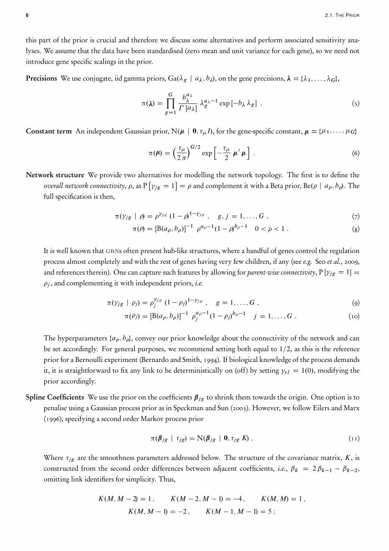
The last move in Section 3 leads to a dramatic decrease in autocorrelation of the Markov chain, compared to a Gibbsmove. Indeed, a common approach in these cases is to use a full Gibbs specification, with a full conditional Bernoullidistribution on the jg and a full conditional Gaussian for the coefficients jg . The latter requires the introductionof a so-called pseudo-prior which needs to be tuned to improve the mixing of the chain (Dellaportas et al., 2000;Ntzoufras, 2002; O’Hara and Sillanpää, 2009). In order to assess the gains in mixing, we implemented a full Gibbssampler for (14). When chain mixing is compared, the advantage of our MH update becomes apparent as illustratedin Figure 1, obtained by running both samplers on the non-linear synthetic data described in Section 4.1. The toppanels plot the number of times that link was switched during the mcmc run against the posterior probability ofthe link being present. One would expect that links with probabilities around 1=2 would change more often, as inFigure 1b. However, the Gibbs strategy tends to mix more slowly, as shown in Figure 1a. Although the MH step ismore computationally demanding, the benefit brought about by the improved mixing of the chain, quantified bythe reduction in autocorrelation (ACF), offsets this cost easily (compare Figure 1c with Figure 1d). Given that theparameter space of the splines model is much larger than the linear one, the benefits of using this move, comparedto the full Gibbs alternative are expected to be even greater.

4. ILLUSTRATIONS AND APPLICATIONS 11

(a) Gibbs strategy. (b) Metropolis-Hastings.

(c) ACF �15, Gibbs strategy. (d) ACF �15,Metropolis-Hastings.

Figure 1. Chain mixing comparison of the Gibbs and MH strategies. Top panels plot the number of state changes ofa link during the MCMC run against its posterior probability. The bottom panels show the autocorrelation function(ACF) for a single link’s precision (gene 15).

4 ILLUSTRATIONS AND APPLICATIONS

Here we illustrate the implementation and performance of our P -splines regression model with three examples.First we analyse two synthetic, discrete time data sets where the data generation mechanism and the topology ofthe network are known. Secondly, we examine a synthetic data set comprising discrete time measurements drawnfrom a continuous time ODE model of a circadian clock. For our last example, we use microarray gene expressiondata from the Arabidopsis thaliana circadian clock.

In all our applications, we include a slight modification of the structure of the network topology to that de-scribed in Section 2.1. We know from the context that each gene has a decay term, corresponding to mRNA decay.We include this information in the prior by fixing gg D 1. As we also know that this decay is close to linear,we set the shape of the inverted Pareto prior for these smoothing parameters to thrice the value used for the rest,i.e. a�gg

D 3 � a�ij; i 6D j .

The splines and linear models were fitted using the overall and gene-wise connectivity specifications. Through-out, 13 bases were used. Prior parameters were set to fa�; b�g= f1=2; 1=2g, fa�; b�g= f2; 0:01g, �� D 1=4, �0 D 0:25

and fa� ; b�g = f1:5; 104g. We ran two parallel chains of length 105, dropping the first 104 steps and then recordingevery tenth draw. We performed some sensitivity analyses, varying a� from 1 (uniform prior) up to 3, settinga� D b� D 1; 2 and using flatter versions of the prior for � by setting a� D 1; 0:1, without finding noteworthydifferences. Convergence was assessed by comparing both chains graphically and by formal tests using the coda

package (Plummer et al., 2006).

4.1 DISCRETE TIME SYNTHETIC NETWORKS

In order to assess the network topology recovery power of our model, we produced two synthetic, first orderautoregressive processes. One has only linear and the second a number of non-linear (S-shaped) relations. In the

12 4.1. DISCRETE TIME SYNTHETIC NETWORKS

non-linear case, all the functional relations were produced using Hill functions, except for the self-interactionswhich are linear. In both cases we set G D 16, T D 40, and � � 0:1.

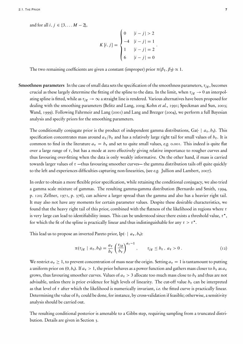
The models with gene-wise and overall connectivity produced almost indistinguishable estimations for thenetwork topology and thus we report the results for the simpler model only. In Figure 2a we plot the marginalposterior and prior distributions of the model precisions, �g (for a selection of the genes only, to avoid clutter). Wealso performed a sensitivity analysis on �, fixing the prior parameters a� D b� D 2. As shown in Figure 2b, theposterior was practically unaffected by this change.

(a) Precision posteriors. (b) Connectivity posterior.

Figure 2. Marginal posterior distributions calculated when fitting the splines model to the non-linear synthetic dataset. (a) The posterior for a selection of the gene precisions, �g and the corresponding prior. (b) The posterior of theoverall-connectivity, �, from two different priors, a� D b� D 1=2 and 2. In both panels priors are depicted by the thick(red) dashed lines.

When the topology of the network is known, we can use the Receiver Operator Characteristic (roc) curve toassess graphically the retrieval performance of a model (Pepe, 2000; Sing et al., 2005). A more formal comparisoncan be carried out by calculating the area under the roc curve (auc): the closer the auc to one, the better theretrieval. For the linear data set these were 0.999 for the fully parametric model and 0.998 with the splines; andwhen fitting the non-linear data set we obtained 0.728 and 0.912, respectively. An alternative measure of fit is the so-called mean cross entropy (MxE), calculated as the Kullback-Leibler divergence from the known network topologyto that estimated by y� , averaged over all possible links. MxE is bounded from below at zero, when the predictedtopology is identical to the real one. Its value for a network topology predicted totally at random, i.e. y ij D 1=2,for all i; j D 1; : : : ; G, is � log 1=2 � 0:7. In the linear network the MxE was 0.042 when fitting the parametricmodel and 0.064 when fitting the splines; with Hill interactions the values were 0.41 and 0.22, respectively.

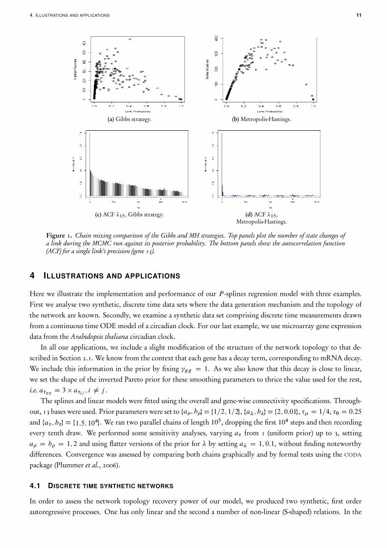
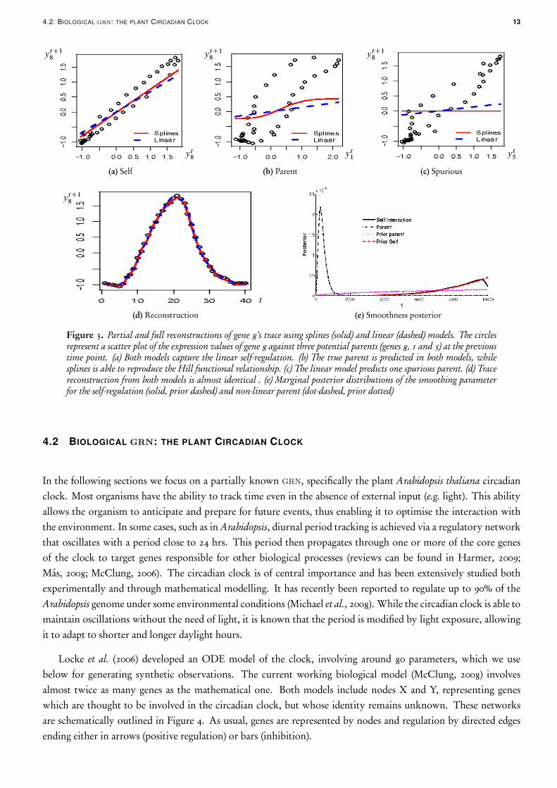
To further understand the differences between the inferred networks under either model, we plot in Figure 3 thepartial and full reconstructions for gene 8’s trace in the non-linear data set, along with the posterior of the corres-ponding smoothing parameter. Both models provide similar predictions, as illustrated by the full reconstructionswhich are practically undistinguishable (Figure 3d). However, the way this fit is achieved varies significantly. Asexpected, both models have a very similar fit for the self-regulation (Figure 3a). As the self-interaction is linear, thesplines model fits it by allocating most of the posterior mass of the corresponding smoothness parameter towardshigh values, depicted as the solid line in Figure 3e. Gene 8 has one parent with a non-linear interaction and thesplines model is capable of reproducing the Hill functional relationship quite precisely (Figure 3b), by allocatingalmost all posterior mass towards small values of the corresponding smoothness parameter, illustrated in Figure 3ewith a dot-dashed line. Obviously, the linear model cannot accommodate such behaviour and may need to includespurious parents in order to compensate for the lack of fit, as in this case, illustrated in Figure 3c by the dashedline with a slight positive gradient. In contrast, the splines model does not predict gene 5 as a parent (solid line inFigure 3c). Notice the mass allocation of the self-regulation link (solid) in Figure 3e: it is basically drawn from theprior (dashed), illustrating that our specification is adequate for linear relations to be reproduced accurately.

4.2. BIOLOGICAL grn: THE PLANT CIRCADIAN CLOCK 13

ytC18

yt8

(a) Self

ytC18

yt1

(b) Parent

ytC18

yt5

(c) Spurious

ytC18

t

(d) Reconstruction (e) Smoothness posterior

Figure 3. Partial and full reconstructions of gene 8’s trace using splines (solid) and linear (dashed) models. The circlesrepresent a scatter plot of the expression values of gene 8 against three potential parents (genes 8, 1 and 5) at the previoustime point. (a) Both models capture the linear self-regulation. (b) The true parent is predicted in both models, whilesplines is able to reproduce the Hill functional relationship. (c) The linear model predicts one spurious parent. (d) Tracereconstruction from both models is almost identical . (e) Marginal posterior distributions of the smoothing parameterfor the self-regulation (solid, prior dashed) and non-linear parent (dot-dashed, prior dotted)

4.2 BIOLOGICAL grn: THE PLANT CIRCADIAN CLOCK

In the following sections we focus on a partially known grn, specifically the plant Arabidopsis thaliana circadianclock. Most organisms have the ability to track time even in the absence of external input (e.g. light). This abilityallows the organism to anticipate and prepare for future events, thus enabling it to optimise the interaction withthe environment. In some cases, such as in Arabidopsis, diurnal period tracking is achieved via a regulatory networkthat oscillates with a period close to 24 hrs. This period then propagates through one or more of the core genesof the clock to target genes responsible for other biological processes (reviews can be found in Harmer, 2009;Más, 2008; McClung, 2006). The circadian clock is of central importance and has been extensively studied bothexperimentally and through mathematical modelling. It has recently been reported to regulate up to 90% of theArabidopsis genome under some environmental conditions (Michael et al., 2008). While the circadian clock is able tomaintain oscillations without the need of light, it is known that the period is modified by light exposure, allowingit to adapt to shorter and longer daylight hours.

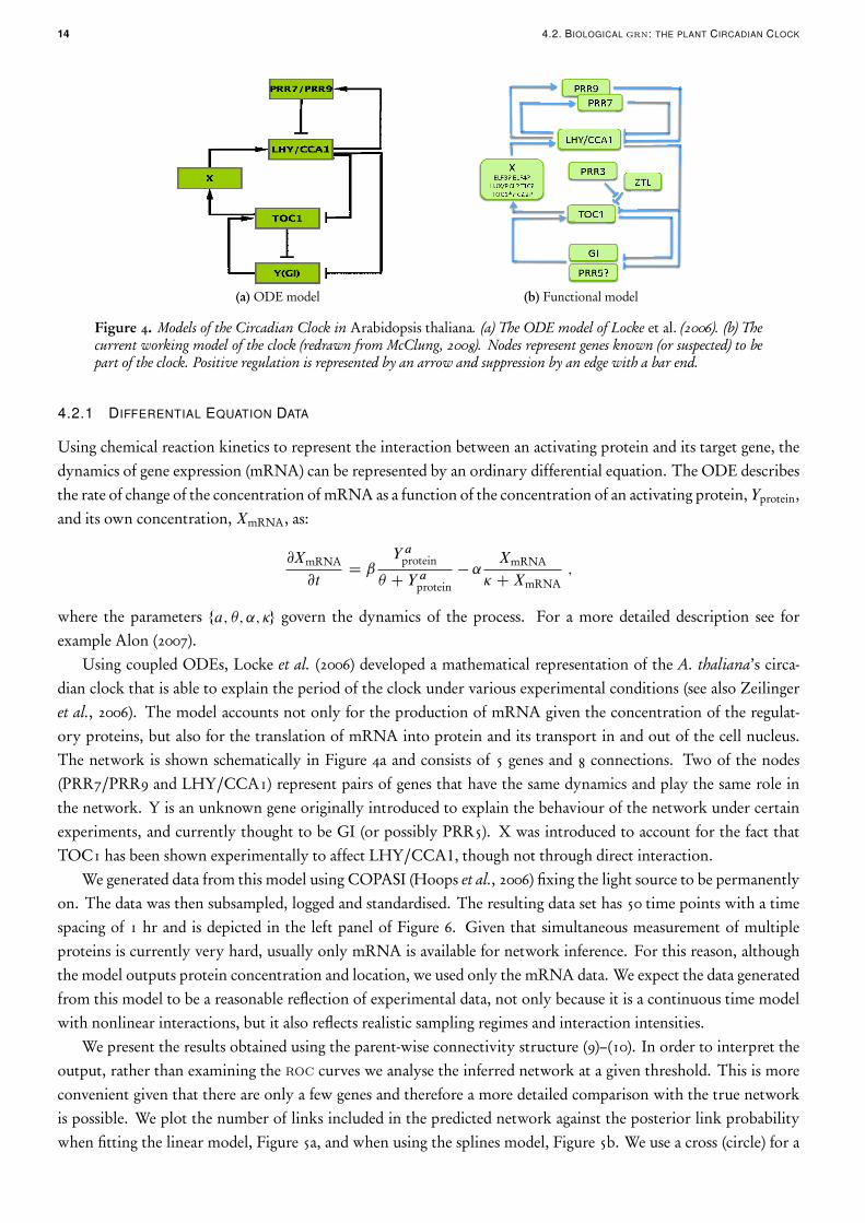
Locke et al. (2006) developed an ODE model of the clock, involving around 80 parameters, which we usebelow for generating synthetic observations. The current working biological model (McClung, 2008) involvesalmost twice as many genes as the mathematical one. Both models include nodes X and Y, representing geneswhich are thought to be involved in the circadian clock, but whose identity remains unknown. These networksare schematically outlined in Figure 4. As usual, genes are represented by nodes and regulation by directed edgesending either in arrows (positive regulation) or bars (inhibition).

14 4.2. BIOLOGICAL grn: THE PLANT CIRCADIAN CLOCK

(a) ODE model (b) Functional model

Figure 4. Models of the Circadian Clock in Arabidopsis thaliana. (a) The ODE model of Locke et al. (2006). (b) Thecurrent working model of the clock (redrawn from McClung, 2008). Nodes represent genes known (or suspected) to bepart of the clock. Positive regulation is represented by an arrow and suppression by an edge with a bar end.

4.2.1 DIFFERENTIAL EQUATION DATA

Using chemical reaction kinetics to represent the interaction between an activating protein and its target gene, thedynamics of gene expression (mRNA) can be represented by an ordinary differential equation. The ODE describesthe rate of change of the concentration of mRNA as a function of the concentration of an activating protein, Yprotein,and its own concentration, XmRNA, as:

@XmRNA

@tD ˇ

Y aprotein

� C Y aprotein

� ˛XmRNA

� C XmRNA;

where the parameters fa; �; ˛; �g govern the dynamics of the process. For a more detailed description see forexample Alon (2007).

Using coupled ODEs, Locke et al. (2006) developed a mathematical representation of the A. thaliana’s circa-dian clock that is able to explain the period of the clock under various experimental conditions (see also Zeilingeret al., 2006). The model accounts not only for the production of mRNA given the concentration of the regulat-ory proteins, but also for the translation of mRNA into protein and its transport in and out of the cell nucleus.The network is shown schematically in Figure 4a and consists of 5 genes and 8 connections. Two of the nodes(PRR7/PRR9 and LHY/CCA1) represent pairs of genes that have the same dynamics and play the same role inthe network. Y is an unknown gene originally introduced to explain the behaviour of the network under certainexperiments, and currently thought to be GI (or possibly PRR5). X was introduced to account for the fact thatTOC1 has been shown experimentally to affect LHY/CCA1, though not through direct interaction.

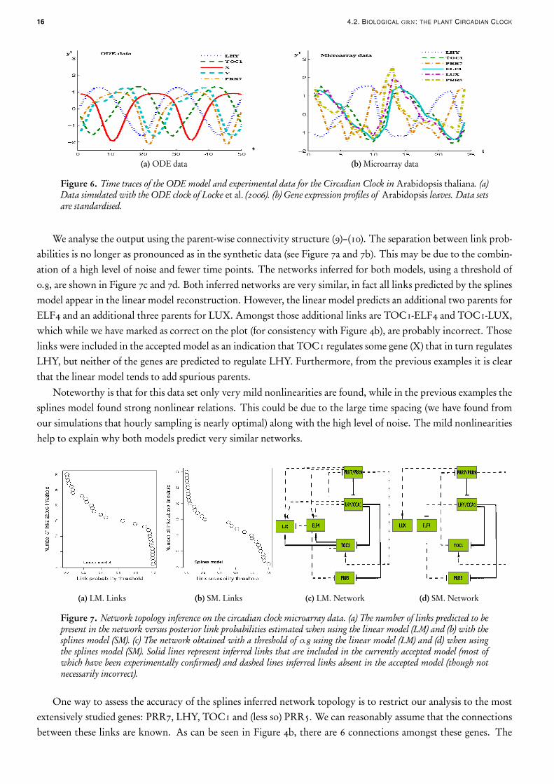
We generated data from this model using COPASI (Hoops et al., 2006) fixing the light source to be permanentlyon. The data was then subsampled, logged and standardised. The resulting data set has 50 time points with a timespacing of 1 hr and is depicted in the left panel of Figure 6. Given that simultaneous measurement of multipleproteins is currently very hard, usually only mRNA is available for network inference. For this reason, althoughthe model outputs protein concentration and location, we used only the mRNA data. We expect the data generatedfrom this model to be a reasonable reflection of experimental data, not only because it is a continuous time modelwith nonlinear interactions, but it also reflects realistic sampling regimes and interaction intensities.

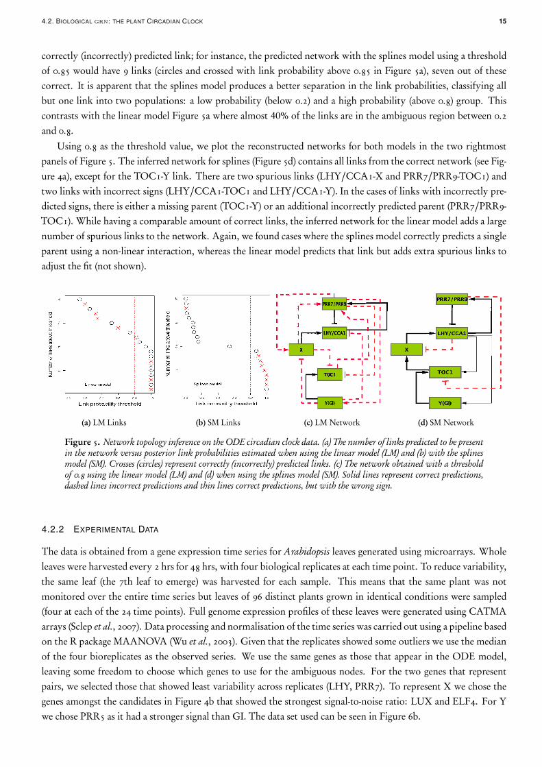
We present the results obtained using the parent-wise connectivity structure (9)–(10). In order to interpret theoutput, rather than examining the roc curves we analyse the inferred network at a given threshold. This is moreconvenient given that there are only a few genes and therefore a more detailed comparison with the true networkis possible. We plot the number of links included in the predicted network against the posterior link probabilitywhen fitting the linear model, Figure 5a, and when using the splines model, Figure 5b. We use a cross (circle) for a

4.2. BIOLOGICAL grn: THE PLANT CIRCADIAN CLOCK 15

correctly (incorrectly) predicted link; for instance, the predicted network with the splines model using a thresholdof 0.85 would have 9 links (circles and crossed with link probability above 0.85 in Figure 5a), seven out of thesecorrect. It is apparent that the splines model produces a better separation in the link probabilities, classifying allbut one link into two populations: a low probability (below 0.2) and a high probability (above 0.8) group. Thiscontrasts with the linear model Figure 5a where almost 40% of the links are in the ambiguous region between 0.2and 0.8.

Using 0.8 as the threshold value, we plot the reconstructed networks for both models in the two rightmostpanels of Figure 5. The inferred network for splines (Figure 5d) contains all links from the correct network (see Fig-ure 4a), except for the TOC1-Y link. There are two spurious links (LHY/CCA1-X and PRR7/PRR9-TOC1) andtwo links with incorrect signs (LHY/CCA1-TOC1 and LHY/CCA1-Y). In the cases of links with incorrectly pre-dicted signs, there is either a missing parent (TOC1-Y) or an additional incorrectly predicted parent (PRR7/PRR9-TOC1). While having a comparable amount of correct links, the inferred network for the linear model adds a largenumber of spurious links to the network. Again, we found cases where the splines model correctly predicts a singleparent using a non-linear interaction, whereas the linear model predicts that link but adds extra spurious links toadjust the fit (not shown).

(a) LM Links (b) SM Links (c) LM Network (d) SM Network

Figure 5. Network topology inference on the ODE circadian clock data. (a) The number of links predicted to be presentin the network versus posterior link probabilities estimated when using the linear model (LM) and (b) with the splinesmodel (SM). Crosses (circles) represent correctly (incorrectly) predicted links. (c) The network obtained with a thresholdof 0.8 using the linear model (LM) and (d) when using the splines model (SM). Solid lines represent correct predictions,dashed lines incorrect predictions and thin lines correct predictions, but with the wrong sign.

4.2.2 EXPERIMENTAL DATA

The data is obtained from a gene expression time series for Arabidopsis leaves generated using microarrays. Wholeleaves were harvested every 2 hrs for 48 hrs, with four biological replicates at each time point. To reduce variability,the same leaf (the 7th leaf to emerge) was harvested for each sample. This means that the same plant was notmonitored over the entire time series but leaves of 96 distinct plants grown in identical conditions were sampled(four at each of the 24 time points). Full genome expression profiles of these leaves were generated using CATMAarrays (Sclep et al., 2007). Data processing and normalisation of the time series was carried out using a pipeline basedon the R package MAANOVA (Wu et al., 2003). Given that the replicates showed some outliers we use the medianof the four bioreplicates as the observed series. We use the same genes as those that appear in the ODE model,leaving some freedom to choose which genes to use for the ambiguous nodes. For the two genes that representpairs, we selected those that showed least variability across replicates (LHY, PRR7). To represent X we chose thegenes amongst the candidates in Figure 4b that showed the strongest signal-to-noise ratio: LUX and ELF4. For Ywe chose PRR5 as it had a stronger signal than GI. The data set used can be seen in Figure 6b.

16 4.2. BIOLOGICAL grn: THE PLANT CIRCADIAN CLOCK

(a) ODE data (b) Microarray data

Figure 6. Time traces of the ODE model and experimental data for the Circadian Clock in Arabidopsis thaliana. (a)Data simulated with the ODE clock of Locke et al. (2006). (b) Gene expression profiles of Arabidopsis leaves. Data setsare standardised.

We analyse the output using the parent-wise connectivity structure (9)–(10). The separation between link prob-abilities is no longer as pronounced as in the synthetic data (see Figure 7a and 7b). This may be due to the combin-ation of a high level of noise and fewer time points. The networks inferred for both models, using a threshold of0.8, are shown in Figure 7c and 7d. Both inferred networks are very similar, in fact all links predicted by the splinesmodel appear in the linear model reconstruction. However, the linear model predicts an additional two parents forELF4 and an additional three parents for LUX. Amongst those additional links are TOC1-ELF4 and TOC1-LUX,which while we have marked as correct on the plot (for consistency with Figure 4b), are probably incorrect. Thoselinks were included in the accepted model as an indication that TOC1 regulates some gene (X) that in turn regulatesLHY, but neither of the genes are predicted to regulate LHY. Furthermore, from the previous examples it is clearthat the linear model tends to add spurious parents.

Noteworthy is that for this data set only very mild nonlinearities are found, while in the previous examples thesplines model found strong nonlinear relations. This could be due to the large time spacing (we have found fromour simulations that hourly sampling is nearly optimal) along with the high level of noise. The mild nonlinearitieshelp to explain why both models predict very similar networks.

(a) LM. Links (b) SM. Links (c) LM. Network (d) SM. Network

Figure 7. Network topology inference on the circadian clock microarray data. (a) The number of links predicted to bepresent in the network versus posterior link probabilities estimated when using the linear model (LM) and (b) with thesplines model (SM). (c) The network obtained with a threshold of 0.8 using the linear model (LM) and (d) when usingthe splines model (SM). Solid lines represent inferred links that are included in the currently accepted model (most ofwhich have been experimentally confirmed) and dashed lines inferred links absent in the accepted model (though notnecessarily incorrect).

One way to assess the accuracy of the splines inferred network topology is to restrict our analysis to the mostextensively studied genes: PRR7, LHY, TOC1 and (less so) PRR5. We can reasonably assume that the connectionsbetween these links are known. As can be seen in Figure 4b, there are 6 connections amongst these genes. The

5. DISCUSSION 17

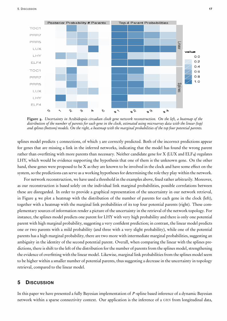
Figure 8. Uncertainty in Arabidopsis circadian clock gene network reconstruction. On the left, a heatmap of thedistribution of the number of parents for each gene in the clock, estimated using microarray data with the linear (top)and splines (bottom) models. On the right, a heatmap with the marginal probabilities of the top four potential parents.

splines model predicts 5 connections, of which 3 are correctly predicted. Both of the incorrect predictions appearfor genes that are missing a link in the inferred networks, indicating that the model has found the wrong parentrather than overfitting with more parents than necessary. Neither candidate gene for X (LUX and ELF4) regulatesLHY, which would be evidence supporting the hypothesis that one of them is the unknown gene. On the otherhand, these genes were proposed to be X as they are known to be involved in the clock and have some effect on thesystem, so the predictions can serve as a working hypotheses for determining the role they play within the network.

For network reconstruction, we have used a threshold in the examples above, fixed rather arbitrarily. Moreover,as our reconstruction is based solely on the individual link marginal probabilities, possible correlations betweenthese are disregarded. In order to provide a graphical representation of the uncertainty in our network retrieval,in Figure 8 we plot a heatmap with the distribution of the number of parents for each gene in the clock (left),together with a heatmap with the marginal link probabilities of its top four potential parents (right). These com-plementary sources of information render a picture of the uncertainty in the retrieval of the network topology. Forinstance, the splines model predicts one parent for LHY with very high probability and there is only one potentialparent with high marginal probability, suggesting a very confident prediction; in contrast, the linear model predictsone or two parents with a mild probability (and three with a very slight probability), while one of the potentialparents has a high marginal probability, there are two more with intermediate marginal probabilities, suggesting anambiguity in the identity of the second potential parent. Overall, when comparing the linear with the splines pre-dictions, there is shift to the left of the distribution for the number of parents from the splines model, strengtheningthe evidence of overfitting with the linear model. Likewise, marginal link probabilities from the splines model seemto be higher within a smaller number of potential parents, thus suggesting a decrease in the uncertainty in topologyretrieval, compared to the linear model.

5 DISCUSSION

In this paper we have presented a fully Bayesian implementation of P -spline based inference of a dynamic Bayesiannetwork within a sparse connectivity context. Our application is the inference of a grn from longitudinal data,

18 5. DISCUSSION

for instance from microarray time series data. Despite being capable of measuring up to tens of thousands ofgenes simultaneously, microarray time series are typically shorter than 20 time points, a consequence of their highcost and the experimental difficulties in obtaining high time resolution. This introduces significant problems foranalysis and modelling, particularly as it limits the complexity of the models that can be used. We addressedthis issue through use of spike-and-slab type priors that, by penalisation implicit in model complexity, limits theconnectivity of the grn. Within this context we are able to increase regression model complexity, providingmethods for exploring whether nonlinear regulatory mechanisms are present in time series data. Our approachis to exploit the flexibility of splines to model arbitrary nonlinear relationships within a first order autoregressiveprocess. We developed a fully Bayesian approach implemented in a (parallelised) mcmc algorithm, and provideappropriate priors such that posterior propriety holds. We found that nonlinear interactions could be successfullyidentified on simulated data (both discrete time and ODE models), the corresponding inferred grn under a linearmodel typically acquiring additional parents, (Figure 3), these incorrectly predicted parents improved the fit toa similar quality to that achieved by the P -splines model. The P -splines model also enhances network sparsitysince an additional parent under a splines regression model incurs a greater penalisation than a parent with a linearfunctional dependence model given its higher (model) complexity; thus even when the links are actually linear thereis stronger control on the number of parents. This compares to artificially imposed parent number penalisation,for instance through an arbitrary weighting exp .�n/ for n parents, as in Kim et al. (2004).

Use of splines in inference requires handling of their functional flexibility. Firstly, there are two fundamentalparameters that define the spline basis —the degree of the spline and the number of knots. The choice of a thirddegree spline is relatively natural and given that we have second order penalties on the coefficients, in the limit as� ! 1, a straight line is obtained. Selecting the number of knots is not as straightforward, but depends on thenumber of time points and the relationship of the time resolution to the time scales in the dynamics. As illustratedby Theorem 1, a large number of knots can affect the stability of the sampler by rendering posteriors close toimpropriety; on the other hand, a small number of knots can seriously affect the flexibility of the spline. Werecommend that the number of knots is much smaller than the number of time points; here we presented resultsusing 10 knots for a time series with 40–50 time points. We found that doubling the number of knots (20) gave severeproblems in the mixing of the chain, while using a smaller number (7) gave similar results. Secondly, the functionalflexibility within the spline basis needs to be controlled; specifically spline degrees of freedom must be constrainedsince otherwise an interpolating spline will be fitted. We use a second order penalisation method that effectivelycontrols the spline curvature. This entails choice of the value of the smoothing parameter � ; previous authorshave optimised and fixed it before estimating the regression. We propose a fully Bayesian approach, inferring itconcomitantly with the regression. Choice of the prior for � is vital since it must allow for cases of both linearityand the levels of nonlinearity implied by the data. The commonly used conditionally conjugate gamma priorspecification is not able to meet both these requirements; we propose the use of an inverted Pareto, which onlyrequires truncating the conditional posterior obtained in the conjugate case. The sole remaining problem is then tofix the value of the cut-off value of the inverted Pareto prior, which can be interpreted as that value after which thefit of the spline is linear. We used a sensitivity analysis to confirm our prior is sufficiently weak, whilst the presenceof predicted linear regulatory links in the inferred network was confirmation that our cut-off was in fact sufficientlyhigh. Network connectivity and spline smoothness were regression/gene specific; this allowed for heterogeneity inthe nonlinearity and parent number across the network.

In biological applications it is known that many regulatory mechanisms are nonlinear (Alon, 2007). However,many grn inference methods use linear models of regulation or implement a restrictive type of nonlinearity, e.g. viadata discretisation and logic gates (Bulashevska and Eils, 2005). Our semi-parametric model thus enables the keyquestion of whether nonlinearity is an important factor in the grn to be addressed. Available gene expressionlongitudinal data for network inference typically comprises 10–100 genes with 10–40 time points, with or without

19

replicates. By standardising the data, the issues facing prior choice are reduced and a generic set of spline parameterswill probably work in most cases. Specifically cubic splines with 10–15 knots and an inverted Pareto prior withshape parameter in (1,2) and a cut-off in

�103; 104

�. A sensitivity analysis in the inverted Pareto prior parameter is

essential, possibly performed on a subset of the data for increased speed, whilst sensitivity to the number of knotsis recommended.

Our algorithm took 2.7 hrs to run 105 iterations with the nonlinear synthetic data (G D 16, T D 40, � � 0:1)and scaling is likely to be quadratic in the number of genes and number of potential parents, and linear in thenumber of time points; for instance, fitting a microarray gene expression data set —not shown— with G D 30

and T D 37 ( O� � 0:15) took 20 hrs for the same run length. Thus, for data sets with a large number of genes aparallel algorithm is available which reduces computation time approximately linearly in the number of cpu-nodes;for instance, using 31 cpus the former data set took 28.6 mins and the later 3 hrs.

Our P -splines model can be extended and modified for specific purposes. Firstly, we model only direct, first-order filiation, i.e. single-parent–child relations. It is well known that for some processes two or more genes need tobind together in order to affect a set of target genes. One can extend the present model for allowing higher degreeinteractions, e.g. by using tensor product splines. The main hindrance would then be the combinatorial growth ofthe topology space, and efficient methods for exploring it must be devised. Secondly, spline coefficient shrinkagecan be performed in a number of ways. We argue that a second order process is natural, given that it constrainsfunction curvature, and thus incorporates linear relations as a special case. However, additional constraints canbe used, including a further term on the prior for the spline coefficients, N.ˇ j 0; !H/, with H derived from thefirst order differences of adjacent coefficients. This effectively penalises large first order differences and favours lessjagged curves, depending on the value of ! > 0. Additionally, the shape of the functional form the spline may takecan also be further restricted. For instance, many gene regulatory effects are monotonic. Extending the model toinclude monotonicity restrictions is feasible by providing such information through a prior (Ansley et al., 1993).Finally, the splines model can be utilised to infer the functional form of the regulation, and coupled with currentbiological knowledge, serve as a basis of a tailor-made parametric model.

ACKNOWLEDGEMENTS

ER Morrissey was supported by the Warwick Systems Biology Doctoral Training Centre. MA Juárez was fundedby bbsrc grant bb/ff003498/1. The experimental data was provided by KJ Denby through the PRESTA Project,grant number bb/f005806/1.

REFERENCES

Ahn, S., Richard, W.T., Park, C.C., Lin, A., Leahy, R.M., Lange, K. and Smith, D.J. (2009) Directed mammaliangene regulatory networks using expression and comparative genomic hybridization microarray data from radi-ation hybrids. PLoS Computational Biology, 5, e1000407. doi:10.1371/journal.pcbi.1000407.

Alon, U. (2007) An Introduction to Systems Biology: design principles of biological circuits. Boca Raton: Chapman &Hall/CRC.

Ansley, C.F., Kohn, R. and Wong, C.M. (1993) Nonparametric spline regression with prior information. Biomet-rika, 80, 75–88.

Bang-Jensen, J. and Gutin, G. (2009) Digraphs : theory, algorithms, and applications. London: Springer, second edn.

20

Bansal, M., Belcastro, V., Ambesi-Impiombato, A. and di Bernardo, D. (2007) How to infer gene networks fromexpression profiles. Molecular Systems Biology, 3, 78.

Belitz, C. and Lang, S. (2008) Simultaneous selection of variables and smoothing parameters in structured additiveregression models. Computational Statistics and Data Analysis, 53, 61–81.

di Bernardo, D., Thompson, M.J., Gardner, T.S., Chobot, S.E., Eastwood, E.L., Wojtovich, A.P., Elliott, S.J.,Schaus, S.E. and Collins, J.J. (2005) Chemogenomic profiling on a genome-wide scale using reverse-engineeredgene networks. Nature Biotechnology, 23, 377–383. doi:10.1038/nbt1075.

Bernardo, J.M. and Smith, A.F.M. (1994) Bayesian Theory. Chichester: John Wiley & Sons.

Biller, C. (2000) Adaptive Bayesian regression splines in semiparametric generalized linear models. Journal of Com-putational and Graphical Statistics, 9, 122–140.

Bonneau, R., Reiss, D., Shannon, P., Facciotti, M., Hood, L., Baliga, N. and Thorsson, V. (2006) The inferelator:an algorithm for learning parsimonious regulatory networks from systems-biology data sets de novo. GenomeBiology, 7, R36+. doi:10.1186/gb-_2006-_7-_5-_r36.

Brezger, A. and Lang, S. (2008) Simultaneous probability statements for Bayesian P-splines. Statistical Modelling, 8,141–168.

Bulashevska, S. and Eils, R. (2005) Inferring genetic regulatory logic from expression data. Bioinformatics, 21,2706–2713. doi:10.1093/bioinformatics/bti388.

Cao, J. and Zhao, H. (2008) Estimating dynamic models for gene regulation networks. Bioinformatics, 24, 1619–1624. doi:10.1093/bioinformatics/btn246.

Chen, L. and Zheng, S. (2009) Studying alternative splicing regulatory networks through partial correlation ana-lysis. Genome Biology, 10, R3. doi:10.1186/gb-_2009-_10-_1-_r3.

Courcelle, J., Khodursky, A., Peter, B., Brown, P.O. and Hanawalt, P.C. (2001) Comparative gene expressionprofiles following UV exposure in Wild-Type and SOS-Deficient Escherichia coli. Genetics, 158, 41–64.

Cowell, R.G., Dawid, A.P., Lauritzen, S.L. and Spiegelhalter, D.J. (1999) Probabilistic Networks and Expert Systems.London: Springer-Verlag.

Damien, P. and Walker, S.G. (2001) Sampling truncated Normal, Beta and Gamma densities. Journal of Computa-tional and Graphical Statistics, 10, 206–215.

Dellaportas, P., Foster, J.J. and Ntzoufras, I. (2000) Bayesian variable selection using the Gibbs sampling. Gener-alized linear models: a Bayesian perspective (D.K. Dey, S.K. Ghosh and B.K. Mallick, eds.). New York: MarcelDekker, 273–286.

Denison, D.G.T., Holmes, C.C., Mallick, B.K. and Smith, A.F.M. (2002) Bayesian methods for nonlinear classifica-tion and regression. Chichester: Wiley.

Denison, D.G.T., Mallick, B.K. and Smith, A.F.M. (1998) Automatic Bayesian curve fitting. Journal of the RoyalStatistical Society B, 60, 333–350.

Dierckx, P. (1993) Curve and Surface Fitting with Splines. Oxford: Clarendon Press.

21

DiMatteo, I., Genovese, C.R. and Kass, R.E. (2001) Bayesian curve-fitting with free-knot splines. Biometrika, 99,1055–1071.

Eilers, P.H.C. and Marx, B.D. (1996) Flexible smoothing using B-splines and penalised likelihood. Statistical Science,11, 89–121. (with discussion).

Fahrmeir, L. and Kneib, T. (2009) Property of posteriors in structured additive regression models: Theory andempirical evidence. Journal of Statistical Planning and Inference, 139, 843–859.

Fahrmeir, L. and Lang, S. (2001) Bayesian inference for generalised additive mixed models based on Markov randomfield priors. Applied Statistics, 50, 201–220.

Faith, J.J., Hayete, B., Thaden, J.T., Mogno, I., Wierzbowski, J., Cottarel, G., Kasif, S., Collins, J.J. and Gardner,T.S. (2007) Large-scale mapping and validation of Escherichia coli transcriptional regulation from a compendiumof expression profiles. PLoS Biology, 5, e8+. doi:10.1371/journal.pbio.0050008.

Fan, J. and Gijbels, I. (1996) Local Polynomial Modeling and its applications. London: Chapman & Hall.

Ferreira, J.T.A.S., Juárez, M.A. and Steel, M.F.J. (2008) Directional log-spline distributions. Bayesian Analysis, 3,267–315.

Friedman, J.H. (1991) Multivariate adaptive regression splines. The Annals of Statistics, 19, 1–141. (with discussion).

Friedman, N. (2004) Inferring cellular networks using probabilistic graphical models. Science, 303, 799–805. doi:10.1126/science.1094068.

Friedman, N., Linial, M., Nachman, I. and Pe’er, D. (2000) Using Bayesian networks to analyze expression data.Journal of Computational Biology, 7, 601–620.

Gardner, T.S., di Bernardo, D., Lorenz, D. and Collins, J.J. (2003) Inferring genetic networks and identifyingcompound mode of action via expression profiling. Science, 301, 102–105. doi:10.1126/science.1081900.

Gardner, T.S., Cantor, C.R. and Collins, J.J. (2000) Construction of a genetic toggle switch in Escherichia coli.Nature, 403, 339–342.

Gentle, J.E. (2003) Random number generation and Monte Carlo methods. New York: Springer-Verlag, second edn.

Gilchrist, M., Thorsson, V., Li, B., Rust, A.G., Korb, M., Roach, J.C., Kennedy, K., Hai, T., Bolouri, H., Aderem,A. and Roach, J.C. (2006) Systems biology approaches identify ATF3 as a negative regulator of Toll-like receptor4. Nature, 441, 173–178. doi:10.1038/nature04768.

Green, P.J. and Silverman, B.W. (1994) Nonparametric regression and generalized linear models: A roughness penaltyapproach. No. 58 in Monographs on Statistics and Applied Probability. Boca Raton: CRC.

Gustafsson, M., Hörquist, M. and Lombardi, A. (2005) Constructing and analysing a large-scale gene-to-gene reg-ulatory network —Lasso-constrained inference and biological validation. IEEE/ACM Transactions on Computa-tional Biology and Bioinformatics, 2, 254–261.

Hache, H., Lehrach, H. and Herwing, R. (2009) Reverse engineering of gene regulatory networks: A comparativestudy. EURASIP Journal of Bioinformatics and Systems Biology, 2009, 1–12. doi:10.1155/2009/617281.

Harmer, S.L. (2009) The circadian system in higher plants. Annual Review of Plant Biology, 60, 357–377.

22

Hartemik, A.J. (2005) Reverse engineering gene regulatory networks. Nature Biotechnology, 23, 554–555.

Hongqiang, L., Lu, L., Manly, K.F., Chesler, E.J., Bao, L., Wang, J., Zhou, M., Williams, R.W. and Cui, Y. (2005)Inferring gene transcriptional modulatory relations: a genetical genomics approach. Human Molecular Genetics,14, 1119–1125. doi:10.1093/hmg/ddi124.

Hoops, S., Sahle, S., Gauges, R., Lee, C., Pahle, J., Simus, N., Singhal, M., Xu, L., Mendes, P. and Kummer, U.(2006) COPASI — a COmplex PAthway SImulator. Bioinformatics, 22, 3067–3074.

Imoto, S., Goto, T. and Miyano, S. (2002) Estimation of gene networks and functional structures between genes byusing Bayesian network and nonparametric regression. Pacific Symposium on Biocomputing, 7, 175–186.

Imoto, S. and Konishi, S. (2003) Selection of smoothing parameters in B-spline nonparametric regression modelsusing information criteria. Annals of the Institute of Statistical Mathematics, 55, 671–687.

Ishwaran, H. and Rao, J.S. (2005) Spike and slab variable selection: frequentist and Bayesian strategies. The Annalsof Statistics, 33, 730–773.

Jaffrezic, F. and Tosser-Klopp, G. (2009) Gene network reconstruction from microarray data. BMC Proceedings, 3,S12. doi:10.1186/1753-_6561-_3-_S4-_S12.

Jensen, F.V. and Nielsen, T.D. (2007) Bayesian networks and decision graphs. New York: Springer, second edn.

Jullion, A. and Lambert, P. (2007) Robust specification of the roughness penalty prior distribution in spatiallyadaptive Bayesian P-splines models. Computational Statistics & Data Analysis, 51, 2542–2558.

Kim, S.Y., Imoto, S. and Miyano, S. (2003) Inferring gene networks from time series microarray data using dynamicBayesian networks. Briefings in Bioinformatics, 4, 228–235.

Kim, S.Y., Imoto, S. and Miyano, S. (2004) Dynamic Bayesian network and nonparametric regression for nonlinearmodelling of gene networks from time series gene expression data. Biosystems, 75, 57–65.

Kohanski, M.A., Dwyer, D.J., Wierzbowski, J., Cottarel, G. and Collins, J.J. (2008) Mistranslation of membraneproteins and two-component system activation trigger antibiotic-mediated cell death. Cell, 135, 679–690. doi:10.1016/j.cell.2008.09.038.

Kohn, R., Ansley, C.F. and Tharm, D. (1991) The performance of cross-validation and maximum likelihood estim-ators of spline smoothing parameters. Journal of the American Statistical Association, 86, 1042–1050.

Lambert, P.C., Sutton, A.J., Burton, P.R., Abrams, K.R. and Jones, D.R. (2005) How vague is vague? A simulationstudy of the impact of the use of vague prior distributions in MCMC using WinBUGS. Statistics in Medicine, 24,2401–2428.

Lang, S. and Brezger, A. (2004) Bayesian P-splines. Journal of Computational and Graphical Statistics, 13, 183–212.

Lauritzen, S. (1996) Graphical Models. Oxford: University Press.

Lèbre, S. (2009) Inferring dynamic genetic networks with low order independencies. Statistical Applications inGenetics and Molecular Biology, 8, Article 9. doi:10.2202/1544-_6115.1294.

Locke, J.C.W., Kozma-Bognár, L., Gould, P.D., Fehér, B., Kevei, E., Nagy, F., Turner, M.S., Hall, A. and Millar,A.J. (2006) Experimental validation of a predicted feedback loop in the multi-oscillator clock of Arabidopsisthaliana. Molecular Systems Biology, 2, 59. doi:10.1038/msb4100102.

23

Marx, B.D. and Eilers, P.H.C. (1998) Direct generalised additive modelling with penalised likelihood. Computa-tional Statistics & Data Analysis, 28, 193–209.

Más, P. (2008) Circadian clock function in Arabidopsis thaliana: time beyond transcription. Trends in Cell Biology,18, 273–281.

McClung, C.R. (2006) Plant circadian rhythms. The plant Cell, 18, 792–803.

McClung, C.R. (2008) Comes a time. Current Opinion in Plant Biology, 11, 514–520.

Michael, T.P., Mockler, T.C., Breton, G., McEntee, C., Byer, A., Trout, J.D., Hazen, S.P., Shen, R., Priest, H.D.,Sullivan, C.M., Givan, S.A., Yanovsky, M., Hong, F., Kay, S.A. and Chory, J. (2008) Network discovery pipelineelucidates conserved time-of-day-specific cis-regulatory modules. PLoS Genetics, 4, e14. doi:10.1371/journal.pgen.0040014.

Mitchell, T.J. and Beauchamp, J.J. (1988) Bayesian variable selection in linear regression. Journal of the AmericanStatistical Association, 83, 1023–1036. (with discussion).

Murphy, K. and Mian, S. (1999) Modelling gene expression data using dynamic Bayesian networks. Tech. rep.,Computer Science Division, University of California, Berkeley.

Ntzoufras, I. (2002) Gibbs variable selection using BUGS. Journal of Statistical Software, 7, 1–19.

O’Hara, R.B. and Sillanpää, M.J. (2009) A review of Bayesian variable selection methods: What, how and which.Bayesian Analysis, 4, 85–118.

Opgen-Rhein, R. and Strimmer, K. (2006) Inferring gene dependency networks from genomic longitudinal data: afunctional data approach. REVSTAT, 4, 53–65.

Opgen-Rhein, R. and Strimmer, K. (2007) Learning causal networks from systems biology time course data: aneffective model selection procedure for the vector autoregressive process. BMC Bioinformatics, 8, S3. doi:10.1186/1471-_2105-_8-_S2-_S3.

Pepe, M.S. (2000) Receiver operating characteristic methodology. Journal of the American Statistical Association, 95,308–311.

Perrin, B., Ralaviola, L., Mazurie, A., Bottani, S., Mallet, J. and d’Alché Buc, F. (2003) Gene network inferenceusing dynamic Bayesian networks. Bioinformatics, 19, ii138–ii148.

Plummer, M., Best, N., Cowles, K. and Vines, K. (2006) CODA: Convergence diagnosis and output analysis forMCMC. R News, 6, 7–11. URL http://CRAN.R-_project.org/doc/Rnews/Rnews_2006-_1.pdf.

Ronen, M., Rosenberg, R., Shraiman, B.I. and Alon, U. (2002) Assigning numbers to the arrows: Parameterizing agene regulation network by using accurate expression kinetics. Proceedings Of The National Academy Of SciencesOf The United States Of America, 99, 10555–10560. doi:10.1073/pnas.152046799.

Ruppert, D. (2002) Selecting the number of knots for penalised splines. Journal of Computational and GraphicalStatistics, 11, 735–757.

Schäfer, J. and Strimmer, K. (2005) An empirical Bayes approach to inferring large-scale gene association networks.Bioinformatics, 6, 754–764. doi:10.1093/bioinformatics/bti062.

24

Sclep, G., Allemeersch, J., Liechti, R., DeMeyer, B., Beynon, J., Bhalerao, R., Moreau, Y., Nietfeld, W., Renou,J.P., Reymond, P., Kuiper, M.T.R. and Hilson, P. (2007) CATMA, a comprehensive genome-scale resource forsilencing and transcript profiling of Arabidopsis genes. BMC Bioinformatics, 8, 400. doi:10.1186/1471-_2105-_8-_400.

Seo, C.H., Kim, J.R., Kim, M.S. and Cho, K.H. (2009) Hub genes with positive feedbacks function as masterswitches in developmental gene regulatory networks. Bioinformatics, 25, 1898–1904.

Shimony, S.E. (1994) Finding MAPs for belief networks is NP-hard. Artificial Intelligence, 68, 399–410.

Sing, T., Sander, O., Beerenwinkel, N. and Lengauer, T. (2005) ROCR: visualizing classifier performance in R.Bioinformatics, 21, 3940–3941. doi:10.1093/bioinformatics/bti623.

Smith, M. and Kohn, R. (1996) Nonparametric regression using Bayesian variable selection. Journal of Econometrics,75, 317–343.

Speckman, P. and Sun, D. (2003) Fully Bayesian spline smoothing and intrinsic autoregressive priors. Biometrika,90, 289–302.

Sun, D. and Speckman, P. (2008) Bayesian hierarchical linear mixed models for additive smoothing splines. Annalsof the Institute of Statistical Mathematics, 60, 499–517.

Toyoshiba, H., Yamanaka, T., Sone, H., Parham, F.M., Walker, N.J., Martínez, J. and Portier, C.J. (2004) Geneinteraction network suggests Dioxin induces a significant linkage between Aryl Hydrocarbon receptor and Re-tionic Acid receptor Beta. Environmental Health Perspectives, 112, 1217–1224.

Wahba, G. (1990) Spline Models for Observational Data, CBMS-NSF Regional Conference Series in Applied Mathemat-ics, vol. 59. Philadelphia: SIAM.

Wand, M.P. (1999) On the optimal amount of smoothing in penalised spline regression. Biometrika, 86, 936–940.

Wand, M.P. and Jones, M.C. (1995) Kernel Smoothing. London: Chapman & Hall.

Wu, H. and Zhang, J.T. (2006) Nonparametric Regression Methods for Longitudinal Analysis. New Jersey: Wiley.

Wu, H., Kerr, M.K., Cui, X. and Churchill, G.A. (2003) MAANOVA: A software package for the analysis of spottedcDNA microarray experiments. The Analysis of Gene Expression Data: Methods and Software (G. Parmigiani, E.S.Garrett, R.A. Irizarry and S.L. Zeger, eds.). New York: Springer, 313–341.

Yin, X., Struik, P.C. and Kropff, M.J. (2004) Role of crop physiology in predicting gene-to-phenotype relationships.Trends in Plant Science, 9, 426 – 432. doi:10.1016/j.tplants.2004.07.007.

Yu, J., Smith, V.A., Wang, P.P., Hartemink, A.J. and Jarvis, E.D. (2004) Advances to Bayesian network inferencefor generating causal networks from observational biological data. Bioinformatics, 20, 3594–3603.

Zeilinger, M.N., Farré, E.M., Taylor, S.R., Kay, S.A. and Doyle, F.J. (2006) A novel computational model of thecircadian clock in Arabidopsis that incorporates PRR7 and PRR9. Molecular Systems Biology, 2, 58. doi:10.1038/msb4100101.

Zellner, A. (1971) An Introduction to Bayesian Inference in Econometrics. New York: Wiley.

Zou, M. and Conzen, S.D. (2005) A new dynamic Bayesian network (DBN) approach for identifying gene regulat-ory networks from time course microarray data. Bioinformatics, 21, 71–79.