Inferring Informed Clustering Problems with Minimum ...davidson/constrained-clustering/...Inferring...
124
Inferring Informed Clustering Problems with Minimum Description Length Principle Ke Yin January 2007 Dissertation submitted in partial fulfilment for the degree of Doctor of Philosophy in Computer Science Department of Computing Science University at Albany
Transcript of Inferring Informed Clustering Problems with Minimum ...davidson/constrained-clustering/...Inferring...
Inferring Informed Clustering Problems with Minimum
Description Length Principle
Ke Yin
January 2007
Dissertation submitted in partial fulfilment for the degree of
Doctor of Philosophy in Computer Science
Department of Computing Science
University at Albany

- ii -
Inferring Informed Clustering Problems with Minimum
Description Length Principle
by
Ke Yin
© Copyright, 2007
- iii -
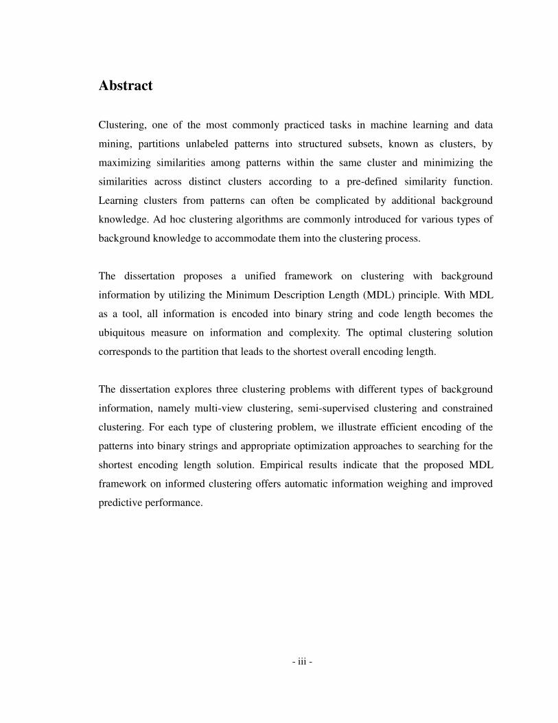
Abstract
Clustering, one of the most commonly practiced tasks in machine learning and data
mining, partitions unlabeled patterns into structured subsets, known as clusters, by
maximizing similarities among patterns within the same cluster and minimizing the
similarities across distinct clusters according to a pre-defined similarity function.
Learning clusters from patterns can often be complicated by additional background
knowledge. Ad hoc clustering algorithms are commonly introduced for various types of
background knowledge to accommodate them into the clustering process.
The dissertation proposes a unified framework on clustering with background
information by utilizing the Minimum Description Length (MDL) principle. With MDL
as a tool, all information is encoded into binary string and code length becomes the
ubiquitous measure on information and complexity. The optimal clustering solution
corresponds to the partition that leads to the shortest overall encoding length.
The dissertation explores three clustering problems with different types of background
information, namely multi-view clustering, semi-supervised clustering and constrained
clustering. For each type of clustering problem, we illustrate efficient encoding of the
patterns into binary strings and appropriate optimization approaches to searching for the
shortest encoding length solution. Empirical results indicate that the proposed MDL
framework on informed clustering offers automatic information weighing and improved
predictive performance.

- iv -
Acknowledgements
The course of writing this dissertation is an arduous one, yet not lonely, because of the
support and encouragement I have been constantly receiving from different groups of
people, without whom the work would be completely impossible.
First and foremost, I am most deeply indebt with my ph.D advisor, Professor Davidson,
who originally motivated me in pursuing a doctoral degree in computer science. During
years of doing research work with him, he has not only imparted the fascinating
knowledge in machine learning and data mining, but also the skill of approaching
problems in a strategic manner. I am also especially grateful that he sacrifices his off-
working hours to advise me on the dissertation, to accommodate my own inflexible
schedule.
I am also fortunate to have the most resourceful committee that I could have asked. The
dissertation involves a spectrum of different fields, including machine learning, statistics
and algorithms. Each of the committee members, Professor Davidson, Professor Stratton
and Professor Ravi brings expertise in the areas and provides precious opinions and
suggestions in shaping the dissertation.
I also owe my thanks to Pat Keller, who has always been so helpful in rescuing me from
administrative problems, when I am on campus and away from campus.

- v -
Finally I cannot express enough gratitude towards my parents, who has always been my
endless source of encouragement and enlightenment, and my beautiful wife Ruowen, for
her considerate understanding and constant supportiveness during the course.

- vi -
Table of Contents
Abstract................................................................................................................................iii
Acknowledgements.............................................................................................................. iv
Table of Contents .................................................................................................................vi
List of Tables ....................................................................................................................... ix
List of Figures....................................................................................................................... x
1 Introduction ..................................................................................................................... 1
1.1 Data Clustering ........................................................................................................ 1
1.2 Informed Clustering Problems................................................................................. 4
1.2.1 Multi-View Clustering ........................................................................................ 4
1.2.2 Semi-Supervised Clustering ............................................................................... 5
1.2.3 Constrained Clustering ....................................................................................... 6
1.3 Minimum Description Length Principle .................................................................. 7
1.4 Dissertation Contribution......................................................................................... 8
1.5 Dissertation Overview ............................................................................................. 9
2 Minimum Description Length ....................................................................................... 11
2.1 Introduction............................................................................................................ 11
2.2 Code....................................................................................................................... 14
2.3 Crude MDL............................................................................................................ 17
2.4 Refined MDL......................................................................................................... 21
2.5 Encoding Continuous Data .................................................................................... 24
2.6 Computation of Stochastic Complexity ................................................................. 24
2.7 Encoding Clustering Data ...................................................................................... 26
2.7.1 Encoding Cluster Assignment........................................................................... 27
2.7.2 Encoding Vector Direction................................................................................ 28
2.7.3 Encoding Vector Length ................................................................................... 28
2.8 MDL and Informed Clustering............................................................................... 30
3 Multi-View Clustering with MDL................................................................................. 31
3.1 Introduction............................................................................................................ 31
3.2 Multiple Views Clustering with MDL ................................................................... 34
3.3 Finding the Optimal Partitions............................................................................... 38
3.4 Empirical Results ................................................................................................... 42
- vii -
3.4.1 Matching Rate (MR)......................................................................................... 42
3.4.2 Predictive Rate (PR) ......................................................................................... 43
3.5 Model Selection ..................................................................................................... 49
3.6 Chapter Summary .................................................................................................. 50
4 Semi-Supervised Clustering .......................................................................................... 51
4.1 Introduction............................................................................................................ 51
4.2 Semi-Supervised Clustering with Mixture Gaussian Model.................................. 53
4.3 Posterior Probability and Model Uncertainty ........................................................ 54
4.4 Bayesian Model Averaging .................................................................................... 55
4.5 Markov Chain Monte Carlo (MCMC)................................................................... 59
4.5.1 Markov Chain ................................................................................................... 59
4.5.2 Metropolis-Hastings and Gibbs Algorithm....................................................... 60
4.6 MDL Coupled MCMC........................................................................................... 61
4.7 Encoding Semi-supervised Clustering with MDL................................................. 62
4.8 MDL Coupled MCMC in Semi-Supervised Clustering......................................... 65
4.8.1 Sample ω........................................................................................................... 66
4.8.2 Sampling z ........................................................................................................ 67
4.8.3 Death and Rebirth ............................................................................................. 68
4.8.4 Split and Combine ............................................................................................ 69
4.8.5 Sampling µ, Σ.................................................................................................... 71
4.8.6 Sampling π ........................................................................................................ 72
The sampling of the multinomial distribution is the same as sampling ω in 4.8.1. ........ 72
4.9 Convergence .......................................................................................................... 72
4.10 MCMC Diagnosis .................................................................................................. 74
4.11 Empirical Results ................................................................................................... 77
4.12 Chapter Summary .................................................................................................. 81
5 Constrained Clustering .................................................................................................. 82
5.1 Introduction............................................................................................................ 82
Instance-Level Constraint ........................................................................................... 83
Cluster-Level Constraint............................................................................................. 84
5.1.1 Model-Level Constraints .................................................................................. 84
5.2 Clustering under Constraints.................................................................................. 86
5.2.1 Feasibility ......................................................................................................... 86
5.2.2 Flexibility.......................................................................................................... 86

- viii -
5.3 Constraints and Codes............................................................................................ 87
5.4 MDL Clustering with Instance-Level Constraints ................................................. 91
5.4.1 Encoding Must-Link Constraints...................................................................... 91
5.4.2 Encoding Cannot-Link Constraints .................................................................. 94
5.4.3 Optimization ..................................................................................................... 96
5.5 Constraints Violation ............................................................................................. 99
5.6 Empirical Results ................................................................................................. 100
5.7 Chapter Summary ................................................................................................ 105
6 Conclusion and Future Work ....................................................................................... 107
References......................................................................................................................... 110

- ix -
List of Tables
Table 2.1 Description Lengths of Binomial Sequence with Different Parameters .................... 20
Table 3.1 MDL Multi-view Clustering on Synthesized Data .................................................... 45
Table 3.2 Two View Clustering Results for Different Digit Pairs ............................................. 46
Table 3.3 Selecting Number of Clustering Within Each View................................................... 49
Table 4.1 Predictive Performance Comparison between SS-OBC and SS-EM......................... 77

- x -
List of Figures
Figure 1.1 An example of K-means clustering on X-Y plane ................................................... 3
Figure 2.1 Kraft’s Inequality ................................................................................................... 15
Figure 2.2 Exact and Asymptotic Parametric Complexity of Binomial Distribution.............. 26
Figure 2.3 Encoding Clustering Data ...................................................................................... 27
Figure 3.1 MDL Based Multi-View Clustering on Image Segmentation. ............................... 48
Figure 4.1 Posterior of a Mixture Gaussian with 8 Labeled Patterns...................................... 56
Figure 4.2 Posterior of a Mixture Gaussian with 4 Labeled and 4 Unlabeled Patterns........... 56
Figure 4.3 Graphical Representation of Mixture Gaussian Model......................................... 63
Figure 4.4 Sampling clustering frequency with constraints, K=4, N=8.................................. 67
Figure 4.5 Mixture Gaussian Model with Four Components and Two Dimensions ............... 75
Figure 4.6 Posterior Distribution of k among different time segments in MCMC chain........ 76
Figure 4.7 Trace Plot of k (Iteration 180000 to 200000)......................................................... 76
Figure 4.8 SS-OBC and SS-EM on Size of Labele Patterns ................................................... 79
Figure 4.9 SS-OBC and SS-EM on Size of Unlabeled Patterns.............................................. 80
Figure 5.1 Encoding with Must-Link Constraints in............................................................... 94
Figure 5.2 Cannot-Link Encoding Auxiliary Graph for .......................................................... 95
Figure 5.3 Performance of UCI Datasets from Different Percentage of Constraints Generated
from Class Labels................................................................................................. 102
Figure 5.4 Performance of UCI Datasets from Different Percentage of Constraints Generated
Randomly ............................................................................................................. 103
Figure 5.5 Comparison between Hard Constraints MDL Selected Soft Constraints on UCI
Datasets from Different Percentage of Constraints Generated from Class Labels
with 40% Noise .................................................................................................... 104
Figure 5.6 Comparison between Hard Constraints MDL Selected Soft Constraints on UCI
Datasets from Different Percentage of Constraints Generated from Class Labels
with 40% Bias ...................................................................................................... 105

- 1 -
1 Introduction
1.1 Data Clustering
Clustering [Har75] [JD88] [JMF99] is one of the most frequently practiced tasks in
machine learning and data mining field. The goal of clustering is to partition a set of
patterns, into finite groups known as clusters, such that the similarity of the patterns are
maximized within the same cluster and minimized across clusters. The importance of
clustering lies in the constructed structure from the otherwise unstructured data, offering
both an explanation on the data generating mechanisms and a predictive device. For
example, a set of mortgage loan borrowers can be partitioned into two clusters based on
their credit score, income, housing value and other information, with one cluster
representing borrowers with high propensity for delinquency and the other for punctual
payments. The structure learnt through clustering process can subsequently predict the
payment behavior of a considered mortgage borrower by comparing profile similarity
between the borrower and each of the learnt clusters. Clustering belongs to the category
of unsupervised learning in the sense that the learner is not coached by the training

- 2 -
patterns with explicit labels, rather, the learner has the freedom of partitioning the
patterns into clusters, each corresponding to an implicit label, hence the name,
unsupervised.
From the perspective of partitioning methodology, clustering falls into two categories,
hierarchical and nonhierarchical. Hierarchical clustering finds the clusters progressively.
It either starts with the entire population as a single cluster, repetitively cleaving larger
clusters into smaller ones, known as the top down approach, or begins with each pattern
as a cluster and incrementally merges them, known as bottom up approach. In contrast,
nonhierarchical clustering partitions all the patterns in a parallel fashion. In this work,
unless explicitly specified, clustering refers to nonhierarchical clustering. Some most well
known nonhierarchical clustering algorithms are K-means clustering and expectation
maximization (EM) on mixture Gaussian models [JD88]. The goal of K-means clustering
is to find partition such that the distortion function, which is the sum of the squared
Euclidean distances of the patterns from the corresponding cluster centers, is minimized.
This is achieved by iteratively assigning each pattern to its closest cluster center via a
greedy algorithm. The algorithm halts when local minimum is achieved and further
iteration does not alter the partition or partition solutions from adjacent iterations are
notably small. Figure 1.1 demonstrates an example of K-means clustering that partitions
150 patterns from X-Y space into three non overlapping clusters.

- 3 -
Figure 1.1 An example of K-means clustering on X-Y plane

- 4 -
1.2 Informed Clustering Problems
Pragmatic clustering problems, however, sometimes involve more complicated situation
than having a set of unlabeled patterns assigned into a fixed number of clusters. Instead,
the learner may have background knowledge on the patterns, which should be considered
into the clustering process. The type of background knowledge can vary by source and
nature. For example, in some problem, partial exterior label may be present for a small
proportion of the patterns to be clustered. A partition of the patterns into clusters must be
consistent with the existing information implied by the labels. While background
knowledge is mostly beneficial in aiding the learner to find more meaningful clusters, it
complicates the clustering process because the additional information it provides does not
automatically falls into the existing clustering framework. In this dissertation, the name
informed clustering is used for all the clustering problems where background
knowledge is imposed. We use a few pragmatic clustering applications to illustrate the
necessity of investigating informed clustering problems.
1.2.1 Multi-View Clustering
A set of patterns sometimes can be described by multiple data sources which constitute
multiple views of the patterns. For example, a database in a commercial bank can have a
table that stores all the demographic information about the mortgage loan borrowers,
including gender, income, credit score, loan purpose, etc. A separate table stores the
monthly payment information such as paid amount and delinquency. Each table is a view
of the patterns (loan borrowers) and can be used to cluster the patterns. Clustering a set of
patterns with more than one view (typically two) is called multi-view clustering [BS04].
- 5 -
The approach to clustering each view independently is insufficient because it does not
utilize the information that the views are describing the same set of patterns. The
independently clustered results would be identical to a problem without the knowledge
that the two views are describing same set of patterns thus the learner has not used all the
information provided. Because the views can potentially be dependent, each view
provides additional information in clustering other views. For this reason, clustering
should be carried simultaneously across the views. Kaski et al. proposed associative
clustering algorithm [KNS+05], with the above stated strategy behind. The algorithm
maximizes the mutual information of the cluster assignments between the views, under
the constraint that each cluster is of Voronoi type, that is, each pattern belongs to its
nearest cluster according to the distance function. The approach is successfully applied in
identifying the dependency between gene expression and regulator binding.
1.2.2 Semi-Supervised Clustering
A second type of informed clustering is semi-supervised clustering. As implied by name,
the problem is the middle ground between supervised and unsupervised learning, such
that the patterns are partially labeled. Partial labeling arises when labeling the entire set
of patterns is too expensive or simply impossible. In some semi-supervised clustering
work, the partial labels are treated as constraints so that patterns with the same class label
form must link constraints and patterns of distinguished class label form cannot link
constraints [BBM02][CCM03]. In other works, the clustering algorithm only have a
preference on assigning patterns with the same explicit labels into the same cluster but
does not enforce it. Instead, a penalty is imposed for heterogeneity of class labels within

- 6 -
the same cluster [GH04].
1.2.3 Constrained Clustering
A third type of informed clustering is constrained clustering. In constrained clustering,
Cluster solutions are bound by a set of rules specified in advance based on either prior
knowledge or problem requirement. The constraints fall into three categories, instance-
level constraint, cluster-level constraint and model-level constraint. The instance level
constraints include must-link and cannot-link constraints. Must-link constraints require
two patterns be assigned to the same cluster; Cannot-link constraints enforce two patterns
not be assigned to the same cluster. Cluster-level constraints enforce the similarity of
patterns within a cluster and dissimilarity of patterns across clusters. Two types of cluster-
level constraints are proposed in [DR05]: the δ-constraint specifies the minimum distance
between any given two patterns from different clusters; the ε-constraint enforces the
maximum distance between any two patterns within a cluster. Model-level constraints are
concerned with clustering solution as a whole, targeting at eliminating dominating
clusters and attributes. The computational complexity of clustering optimization under
constraints may increase significantly with the quantity and complexity of constraints.
Davidson and Ravi investigated the computational complexity of deciding cluster
feasibility under instance-level and cluster-level constraints [DR05].
In addition to the challenges imposed on each informed clustering problem introduced
above, they also inherit some of the challenges from the original clustering problems such
as deciding the number of clusters. Most clustering algorithms assume known cluster

- 7 -
numbers, which is justified when the learner has that prior knowledge. However, under
certain circumstances, it is desirable to allow the patterns themselves to inform the
learner about the number of clusters. Choosing number of clusters is even more
demanding in informed clustering, where the solution must accommodate the background
knowledge in the problem.
The key approach to solving the informed clustering problem is to combine information
from different types and reach a clustering solution that comprehensively summarizes all
the information. This involves deciding the importance and relevance of information, and
the tradeoff among them. For example, in semi-supervised clustering, although it is
desirable to have patterns with the same class labels assigned to the same cluster, it
should not be achieved by sacrificing too much on the cluster qualities, which can be
measured by the similarity of patterns within a cluster. The same rationale applies in
deciding the number of clusters: while incrementing the cluster number always improves
the similarity among the clusters, the dissimilarity across the clusters will be reduced thus
lead to potentially worsened clustering partition. As a consequence, various type of
information needs to be computed, combined and optimized simultaneously in informed
clustering. However, the various types of information are not immediately combinable, as
the scale and unit measuring them are not directly comparable.
1.3 Minimum Description Length Principle
The learning by compact encoding theories [WF87] [Ris87] avail themselves as tools to
measure information in a ubiquitous way. In the theories, all types of information, of
- 8 -
patterns, of clusters, of secondary view, of partial labels or of constraints, are measured in
the same unit by encoding the information into binary strings, the lengths of which are
the sole measurement on the information amount. There are two branches in the learning
by compact encoding theories, namely minimum message length (MML) and minimum
description length (MDL). The two theories share the same philosophical insights but
with subtle nuances. MML constructs a code with two steps: the first step encodes a
theory from a countable set of theories, which is similar to the subjective prior in
Bayesian with discretization; the second step constructs a code for the data with the
presence of knowledge from the already encoded theory. The inferred theory in MML is
the one that minimizes expected total code length within a theory. In contrasts, MDL
allows one part message encoding and the complexity of a theory is represented by the
entire theory set rather than individual theories. In addition, the MDL inference is the one
that minimize the expected code length over all possible data. In this work, we choose
MDL as the inference tool for the convenience of one part code.
1.4 Dissertation Contribution
The dissertation establishes a unified framework for informed clustering with MDL as a
tool. It makes the following contributions into the current research on informed
clustering:
1. It provides a unified framework for informed clustering problems which optimize
information weighing and complexity tradeoff, offering inference methodology on
informed clustering problems with improved empirical predictive capability.
2. The work develops efficient encoding for the three informed clustering problems
- 9 -
mentioned. For each of the three informed clustering problems, the work derives the
description length function and applies different optimization techniques in searching
for the solution.
3. As the framework utilizes MDL, it automatically addresses the model selection
problem in informed clustering, which is otherwise not frequently addressed.
1.5 Dissertation Overview
The chapters of the dissertation are to be organized in the following manner: Chapter 2
provides a brief introduction to the MDL principle and related literature. It discusses the
relationship between probability and codes, encoding discrete and continuous data, two
parts and one part MDL encoding, and encodings for some commonly encountered
distributions, which serve as building blocks for subsequent chapters. Chapter 3 focuses
on multi-view clustering problem. The chapter explores the encoding, optimization of the
multi-view clustering problem with MDL principle. Dependency information among the
views can be captured by encoding the views simultaneously, which offers superior
clustering solutions to clustering the views independently, as indicated by various
empirical results. Chapter 4 addresses semi-supervised clustering problem, where the
patterns are partially labeled. The chapter explores mixture Gaussian model and establish
the MDL encoding method. MDL coupled Markov chain Monte Carlo (MCMC)
sampling is introduced and applied in searching for the clustering solutions. Chapter 5
concentrates on clustering problems under constraints. The chapter discusses how
constraints as background knowledge can be exploited in shortening the overall encoding
length. Also the chapter develops criteria in identifying “good” constraints that improves

- 10 -
the learning and “bad constraints” that deteriorates the learning. Chapter 6 summarizes
preceding chapters and overviews informed clustering problems from a high level to
yield a unified framework. The chapter concludes the dissertation and state further
investigation directions.

- 11 -
2 Minimum Description Length
2.1 Introduction
In machine learning, a problem that often confronts the learner is to choose among
multiple theories that seemingly consistent with the observed data, known as the model
selection problem. Deciding the number of clusters is an example of model selection
problem in the clustering context. A model that provides the best fitting is not necessarily
the best model that captures most insight from the data. For example, in K-means
clustering, model fitting is typically measured by the quantization error, the sum of the
squared distances of all patterns from their allocated cluster centers. A smaller
quantization error represents greater homogeneity within clusters and indicate better
fitting. However, a trivial clustering solution that assigns each pattern into its own cluster
has zero quantization error, yet it is obvious that no insight is gained from the model.
Because a complicated model typically provides more flexibility and allows better fitting
to the data, the improvement in fitting should be penalized with increased model

- 12 -
complexity, as stated by the famous Occam’s razor, that “entities should not be multiplied
beyond necessity”.
How does one achieve the optimal trade-off between better data fitting and controlled
model complexity? If the two are measured in the same unit, then a single objective
function can be computed by combining the two and the best model minimizes the
function. One method to realize the idea is by encoding both the model and data into
binary strings, and measuring the total complexity as the lengths of the encoded strings.
The encoded strings should be lossless compressions of the original data by exploiting
the regularities. If the description length of the data with the aid of a model is shorter than
that without, then the model has offered new knowledge in the data. Two similar theories
have been derived from this philosophy, the minimum message length (MML) principle
and the minimum description length (MDL) principle. While the concepts are similar, the
two theories have some subtle and important differences.
The MML principle [WB68] [WF87] is first proposed by Wallace and Boulton in 1968.
MML divides the model parameter space into discrete cells and place a prior distribution
upon them. From the distribution, the parameters can be encoded up to a precision
defined by the dimension of the cell. The data is then encoded with the knowledge of
model. An optimal precision can be derived by minimizing the expected two parts
message length over the parameter cell: if the precision is high, it takes longer message to
encode the model parameters but the message length encoding the data can be reduced;
on the other hand, a low precision enables shorter message encoding the model

- 13 -
parameters but lengthening the second part of the code. If the model parameter set is
countable where no discretization is necessary, the actual message length rather than the
expected message length is minimized. MML principle has been applied widely in
machine learning problems. Wallace et al used MML to prevent over-fitting in decision
tree classifier [WP93]; Oliver and Baxter developed a MML-based unsupervised learning
framework [BO00]; Davidson proposed Markov chain Monte Carlo sampling in
clustering problem where the full conditional probability is derived from the MML
computation [Dav00]. Fitzgibbon, Allison and Dowe suggest the usage of MML in
clustering ordered data [Fad00].
The MDL principle is developed by Rissanen independently in a series of papers [Ris78]
[Ris87] [Ris01]. The early stage MDL is similar to MML, adopting a two part encoding
method. The major difference between the two part MDL and MML is that MDL does not
acknowledge a subjective prior, rather, it advocates non informative prior such as
Jeffery’s prior on the model parameters. However, different priors still lead to different
encoding on the models and thus possibly different model selection outcomes. The two
part MDL, also referred as the crude MDL, is refined into one part MDL when the
normalized maximum likelihood (NML) distribution is introduced to encode the data.
The NML encoding is a universal code where the encoding for any encountered data is
almost as short as can be achieved by the maximum likelihood code. Furthermore, the
code length representing the model complexity does not depends on particular model
parameters anymore; instead it is a fixed encoding cost that is only pertinent to the
“richness” of model. Both crude MDL and refined MDL have received numerous

- 14 -
applications. It has been used in efficient decision tree pruning which yields in improved
predictive accuracy [QR89] [MRA95]. In unsupervised learning, Kontkanen et al has
developed efficient recursive computation of one part MDL for multinomial distribution
[KMB+03] and apply it in the clustering framework [KMB
+05].
This chapter introduces minimum description length principle and its applications in
plain clustering, which serves as the basics for the subsequent chapters.
2.2 Code
We define a code as a mapping from a countable set S to a set of finite binary strings,
with each mapped binary strings called a code word. A prefix code is a code where no
code word is a prefix of another. For example, A, B, C, D→00, 01, 10,11 constitutes
a prefix code while A, B, C, D→1, 10, 110, 111 does not. The significance of prefix
code is that the decoding process requires no additional delimiter and can be done
unambiguously.
In MDL principle, one is only concerned with the length of the codes rather than the
contents themselves. For prefix code, the code word lengths must satisfy certain
mathematical properties. Let LC: S→R+ denotes the function computes to code length for
Ss ∈ with prefix code C. In the above prefix example, the code lengths are the same for
all four symbols in the set, LC(A)= LC(B)= LC(C)= LC(D)=2. As the goal in MDL is to
shorten the message length, a natural question to ask is how short LC can be while the
code is still decodable, which is answered by Kraft’s inequality.

- 15 -
Kraft’s Inequality: For a prefix code C that encodes a finite set S with an alphabet of
size r with encoding length function LC, the following inequality holds:
( )1≤∑
∈
−
Ss
sLCr (2.1)
Conversely, for any encoding length function LC that satisfies the inequality, a prefix code
mapping from S to an alphabet of size r can be constructed.
Figure 2.1 Kraft’s Inequality
The correctness of Kraft’s inequality can be illustrated by explicitly constructing an r-ary
tree as illustrated in Figure 2.1 for code C, where each node represents a symbol in the
alphabet thus each path from root to leaf represents a code word. By the nature of the
construction, the code is prefix. Let d be the depth of the tree. For a code word s1 with
length LC(s1), the leaf node can be potentially expand into a sub-tree with ( )1sLd Cr
− leaf
nodes. However the sum of all the leaf nodes expanded from the current tree should not
exceed to maximum number of leaf nodes for a tree with depth of d,

- 16 -
( ) d
Ss
sLdrr C ≤∑
∈
−
1
1 (2.2)
The Kraft’s inequality follows. Conversely, given a description length function LC that
satisfies Kraft’s inequality, one can always construct a tree in the same manner such that
the number of leaf nodes equals the size of the alphabet and the depth of the nodes
corresponds to the lengths of the descriptions.
An immediate implication of Kraft’s inequality is that a code that used by MDL which
yields the shortest description length must satisfy the equality condition. If not, the code
length of certain symbol in set S can be shortened so that the equality is established.
Thus, only efficient prefix code that satisfies the equality condition is the candidate code
that corresponds to the shortest description length. For an efficient prefix code,
( )1=∑
∈
−
Ss
sLCr (2.3)
Equation (2.3) states that an efficient prefix code corresponds to a probability measure on
set S. It is easy to verify that
( ) ( )sLCrsP−= (2.4)
satisfies the three conditions for probability measure: non-negativity, unity and countable
additivity. A probability distribution implies a code length function and vice versa. For a
probability measure P on S, a unique efficient code length function can be constructed,
( ) ( )sPsL rC log−= (2.5)
Although the code length function LC is unique, potentially more than one efficient prefix
code can be constructed to satisfy the function. However, as MDL is only concerned with
code length, they are considered indistinguishable and yield the same inference.

- 17 -
2.3 Crude MDL
With a known probability measure on a finite symbol set S of size r, the one-to-one
correspondence between probability measure P and efficient prefix code in section 2.2
offers a straightforward computation of the description length required to encode data D
of length N composed with symbols from S. Let ( )snD be the number of times a symbol
appeared in data, the description length is
( ) ( ) ( )∑∈
−=Ss
rD sPsnPL log (2.6)
We want to minimize L (P) regarding to P subject to the constraints
( ) ( ) 0,1: >=∑∈
sPsPPSs
(2.7)
The Lagrange multiplier here is
( )( ) ( ) ( ) 01log =
−+−
∂
∂∑ ∑∈ ∈Ss Ss
rD sPsPsnsP
λ (2.8)
This gives
( )( )
0ln
=+− λsP
rsnD (2.9)
Substituting to the constraint that probability sum up to one,
( ) ( ) ( )∑∑∑∈∈∈
====SsSsSs
snNrN
rsnsP where,1ln
ln1
λλ (2.10)
Solving λ and substituting back to the Lagrange equation, the probability that minimizes
the description length function is
( ) ( )N
snsPD =* (2.11)
and the corresponding shortest description length is

- 18 -
( ) ( )( )
∑∈
−=Ss
D
DDN
snsnrPL lnln* (2.12)
Two observations can be made from the results. First, the size of the set r plays the role of
regulating the description length unit, which does not affect the minimization process.
For mathematical convenience, e will be used for the rest of the dissertation. Second, the
probability measure that leads to the shortest description length of the data is the relative
frequency of each symbol within the data. Shorter code words are reserved for more
frequently appeared symbols.
The above computation defines a code on all possible data with length N. For any data
string D of length N, we first compute the probability measure that leads to the shortest
description length, which is defined by the relative frequency of symbols in D. From the
probability measure, we construct an efficient code on set S and use it to encode each
symbol in D. Unfortunately such a code is not decodable by the receiver to recover D as
the decoding the probability measure that encodes D depends on D itself. This is revealed
by computing the left hand side of Kraft’s inequality on all possible data with length N
( ) ( ) ( ) 111
* =
=> ∑∑ ∏∑ ∏
∈∈ =∈ =
N
Ss
A
SD
D
Ds
A
SD
D
Ds
D sPsPsPN
N
N
N
(2.13)
PA here is an arbitrary prefix code on S that is fixed to encode all possible data D from SN.
The first inequality set holds strictly for all N greater than 1. The second equality sign
comes from the multinomial theorem. The violation of Kraft’s inequality states that
relative frequency code is not a prefix code SN.

- 19 -
The situation is mended by constructing a two part code: the first part of the code encodes
the probability measure used to encode the subsequent data. The encoded probability
measure can be regarded as theory H. The second part encodes the data SN with the
knowledge of theory H. To construct each part of code, one only needs to construct the
corresponding marginal probability distribution on H and the conditional probability of
SN given H. The model of choice in MDL inference is the one that minimizes the total
two parts description length
( ) ( ) ( )
( )hLh
hSPhPhL
HhMDL
N
∈
=
−−=
minarg
|lnln
(2.14)
Example 2.1 (Binomial Sequence): Let 1,0=S . The data is a binary string with
length N that may contain certain regularities. Let )1,0(: →Shp be a probability
measure on S with ( ) ( ) phph −== 11,0 . Further let H be a set of h such
that
= 1,...,10
2,
10
1,0p . The agreed marginal probability distribution on H between the
sender and receiver is ( ) phP p11
2= . For any particular given data string S
N, the sender
chooses the theory that minimizes the two parts description length. The total description
length is computed as
( ) ( ) ( ) ( )pnpnp
hL p −−−−= 1ln1ln011
2ln (2.15)
Following table illustrates the description lengths of various probability measures for data
with length 10 and length 100.

- 20 -
Table 2.1 Description Lengths of Binomial Sequence with Different Parameters
The MDL inference on the first data is p=0.5 and inference on the second data is p=0.4.
When the observed data is short, MDL prefers “simpler” model that requires less
description length but for longer data, the fitness of the model on the data starts to
dominate. More complex model is only used until enough data makes it necessary, which
is consistent with Occam’s razor philosophy.
While the conditional probability of the data given the model, which decides the second
part of the description, is usually unambiguous and defined by the set of probability
measure under consideration, the marginal probability which corresponds to the first part
of the description is more subjective. With extreme specification of the marginal
probability distribution on the model class H, one may infer any model desired, by
concentrating probability mass on certain model. Even if one only restrict to objective
priors such as Jeffery prior, it is not immediately clear whether a prior represents a model
complexity well. A prior that encodes some data efficiently could potentially be very
redundant in encoding some other data. This drawback on the crude MDL calls for
universal coding where the code should perform close to optimal for different possible
data.
p 0 0.1 0.2 0.3 0.4 0.5
n(0)=4,n(1)=6 Inf 13.85 11.09 9.86 9.35 9.33
n(0)=40,n(1)=60 Inf 102.4 81.08 72.47 69.92 71.71
p 0.6 0.7 0.8 0.9 1
n(0)=4,n(1)=6 9.76 10.71 12.48 16.05 Inf
n(0)=40,n(1)=60 77.63 88.57 107.4 144.2 Inf

- 21 -
2.4 Refined MDL
As mentioned above, the major difficulty in crude MDL approach is to encode the model
so that the code performs well on all data. The maximum likelihood code, although
always leads to the shortest possible second part description length, does not constitute a
prefix code over all possible data. A natural question becomes, does a prefix code exist
that is only slightly longer than the maximum likelihood code over all possible data. Such
a prefix code is called a universal code. The increase in code length compared to the
maximum likelihood code is called regret.
Definition 2.1(Regret): Given a class of codes C, the regret of a prefix code Q relative to
C for data NSD ∈ is defined as
( ) ( ) ( ) ( ) ( )DPDQDPDQDQR DP
*lnlnlnmaxln, +−=−−=∈C
(2.16)
*
DP is the non prefix maximum likelihood code on NS . The regret is the extra description
required for Q to encode D to make Q decodable. The regret is a function of both the
code Q and the encountered data D. For a given code Q and data D, the regret can be
large or small. A good code Q optimizes the worst case scenario, minimizing the largest
regret over all possible data,
( ) ( ) ( )DQRQRDQNSDQQ
,maxminargminarg max
*
∈== (2.17)
Theorem 2.1 (Normalized Maximum Likelihood Code) The code that minimizes the
maximum regret is
( )( )
( )∑∈
=
NN
N
Ss
N
s
D
sP
DPDQ
*
**
(2.18)

- 22 -
Proof: The max regret for Q* is a constant that does not depend on D
( ) ( ) ( ) ( ) ( )∑∑∈∈
=++−=NN
N
NN
N
Ss
N
sD
Ss
N
sDD
sPDPsPDPDQR***** lnlnlnln,max
For an arbitary code *QQ ≠ , there must exist a data sequence that ( ) ( )NN sQsQ *< , the
regret difference on Ns is
( ) ( ) ( ) ( ) ( )( )
0lnlnln,,*
** <=−−−=−N
NNNNN
sQ
sQsQsQsQRsQR
Thus ( ) ( )DQRDQRDD
,max,max * <
Q.E.D.
( )DQ* is known as the normalized maximum likelihood (NML) distribution on D. Thus
the code derived from it is a prefix code on D that allows encoding all possible data
efficiently. The description length of data D with the NML code is
( ) ( ) ( )DPsPDL D
Ss
N
sNMLNN
N
** lnln −= ∑∈
(2.19)
The second term is the maximum likelihood code that represents the fitness of the code
on the data. The first term is a constant across all data for a given code class C and
represents the complexity of the code class, known as the Parametric Complexity (PC) of
the class. The total encoding length, the parametric complexity plus the likelihood code
cost, is known as the Stochastic Complexity (SC).
The computation of parametric complexity can be a tedious and difficult task. When the
code class C is parametric, if the stochastic complexity is finite and C belongs to an

- 23 -
exponential family, the parametric complexity can be approximated by its asymptotic
form [Ris96],
( ) ( ) ( )1ln2
ln2
, odINk
NPC ++= ∫Θ∈
θθπ θ
C (2.20)
Where k is the number of parameters and ( )θI is the Fisher information matrix where the
(i, j) entry is computed as
( ) ( )
∂∂
∂−= θ
θθθ |ln
2
, DPEIji
Dji (2.21)
The first term of the asymptotic form of stochastic complexity computes the complexity
contributed by the number of parameters, the form of which is consistent with Bayesian
Information Criterion (BIC). However, measuring complexity by number of parameters
alone is not sufficient. Both a Gaussian model and a uniform model have two parameters
but the data representation capacities are different. This “richness” of a model space is
captured by the second term derived from Fisher information matrix.
The one part MDL offers immediate guide on the model selection problem. Given two
model classes, parametric complexity represents the complexity term of a model class
and maximum likelihood code captures the goodness of the fit to the data. The sum of the
two, stochastic complexity, offers the yardstick in the model selection problem. The
model of choice is the one that minimizes the stochastic complexity.

- 24 -
2.5 Encoding Continuous Data
If data to be encoded is continuous, where the probability for a particular member is zero,
the corresponding encoding length becomes infinity. Hence continuous data can only be
encoded to a certain precision. Let x be a real number and let f be a continuous
probability measure on the real numbers. The probability of x with precision ε is
( ) ( ) ( )xfdxxfxx
xε
ε
ε ≈= ∫+
−
2
2
Pr (2.22)
The corresponding description length becomes
( ) ( ) εε lnln, −−= xfxL f (2.23)
In minimizing the description length regarding to f, the choice of precision becomes
irrelevant. By assuming all codes use the same infinitesimal precision, the relative
description length is simply ( ) ( )xfxL f ln−= by dropping the precision term. The
relative description length can potentially be negative if the probability density of x is
larger than one. In this scenario, it is sufficient to remember that the actual description
length is always positive and the negative description function is the original description
length less a constant where they share the same MDL estimators.
2.6 Computation of Stochastic Complexity
The computation of stochastic complexity involves integrating maximum likelihood over
the entire data space and can be a tedious and time consuming task. When the asymptotic
form applies, it facilitates the computation significantly. For large data size N and fixed
number of parameters, the term contributed by Fisher information matrix becomes

- 25 -
insignificant and stochastic complexity reduces to Bayesian information criterion.
However, MDL is significantly different from BIC when k and N are of comparable
magnitude.
Example2.2 (Binomial Sequence): The probability mass function for a binomial
distribution is given by
( )( )
( ) nNn ppnNn
Npnf
−−
−= 1
!!
!; (2.24)
The determinant of the Fisher information matrix is
( )( )pp
pI−
=1
1 (2.25)
The asymptotic form of the parametric complexity can thus be computed as
( )( )
( ) ( )12
ln2
1ln
2
11
1
1ln
2ln
2
1,
1
0
oNodppp
NNPC ++=+
−+= ∫
π
πP (2.26)
It is also impossible to compute the stochastic complexity exactly by exhaustively
summing up the maximum likelihood over all possible data. Kontkanen et al [KMB+03]
proposed an efficient recursive method that allows computing the parametric complexity
at ( )SNO ln2 . For the binomial example, the exact parametric complexity and the
asymptotic parametric complexity are compared in Figure 2.2. For practical purposes, the
asymptotic form is good approximation of the exact form.

- 26 -
0
0.5
1
1.5
2
2.5
3
0 20 40 60 80 100 120
Exact Asymptotic
Figure 2.2 Exact and Asymptotic Parametric Complexity of Binomial Distribution
2.7 Encoding Clustering Data
For parameterized clustering algorithms such as K-means clustering, the MDL principle
introduced above is immediately applicable once a prefix code on the data is designed
within the clustering framework. For example, in K-means clustering, a pattern can be
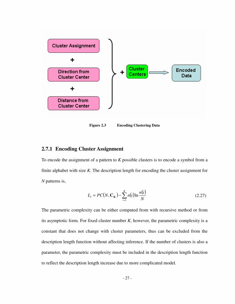
encoded with three parts of description indicated below.
The first part describes the cluster assignment of the pattern. This part combined with the
cluster parameters constitutes the basis for subsequent descriptions. The second part and
third part describes the direction and distance of the vector from the pattern to the cluster
center. Three parts descriptions together fully encode a pattern in the data space.
- 27 -
Figure 2.3 Encoding Clustering Data
2.7.1 Encoding Cluster Assignment
To encode the assignment of a pattern to K possible clusters is to encode a symbol from a
finite alphabet with size K. The description length for encoding the cluster assignment for
N patterns is,
( ) ( ) ( )∑
=
−=K
i N
ininNPCL
1
1 ln, KC (2.27)
The parametric complexity can be either computed from with recursive method or from
its asymptotic form. For fixed cluster number K, however, the parametric complexity is a
constant that does not change with cluster parameters, thus can be excluded from the
description length function without affecting inference. If the number of clusters is also a
parameter, the parametric complexity must be included in the description length function
to reflect the description length increase due to more complicated model.

- 28 -
2.7.2 Encoding Vector Direction
In K-means clustering, the Euclidean distances from the patterns to the cluster centers are
treated equally regardless of the directions of the corresponding vectors they are
computed from. This allows constant encoding length of the vector direction from the
patterns to the cluster centers, which can be excluded from the description length
function.
2.7.3 Encoding Vector Length
In K-means clustering, the Euclidean distance from a pattern x to its cluster center Cx is
computed as
2
xCxr −= (2.28)
The objective of K-means clustering is to minimize the sum of the Euclidean distances
over all patterns. The prefix code to encode the distances must also reflect this
preference, reserving succinct code words for short distances and redundant code words
for large distances. One code of choice is the exponential distribution, whose probability
density function is
( )
−=
σσσ
rrf exp
1; (2.29)
For N patterns with Euclidean distances Nrr ,...,1 , the total length of the code as the
function of the distances is,
( ) ( )NPCNr
rrLN
i
i
N ,ln,...,1
1 σ++=∑=
σσ
σ (2.30)
The maximum likelihood code is obtained by maximizing σL over σ ,

- 29 -
N
rn
i
i∑== 1*σ
(2.31)
Substitute the maximum likelihood estimator, the stochastic complexity the exponential
distribution model is
( ) ( )NPCN
r
NNrrL
N
i
i
n ,ln,..., 1
1* σ++=∑
=
σ
(2.32)
The Fisher information determinant of the model is,
( )2
1
σσ =I (2.33)
The asymptotic form of the parametric complexity suffers the infinity problem,
( ) ∞=∫∞
0
σσ dI (2.34)
The problem can be solved by restricting our model space to [ ]maxmin ,σσσ ∈ , the
parametric complexity becomes,
( ) ( ) ( ) ( )1lnln2
ln2
11ln
2ln
2,
min
maxmax
min
oN
odINk
NPC ++=++= ∫ σ
σ
πσσ
π
σ
σ
σ (2.35)
The total description length of K-means clustering is the sum of all three parts,
( ) ( ) ( ) ( )NPCN
r
NNN
ininNPCL
N
i
iK
i
meansK ,lnln, 1
1
σCK +++−=∑
∑ =
=−
(2.36)
In the description length function, both the cluster frequencies ( )in and the Euclidean
distances ir can be deterministically computed once the cluster partition is decided. The
MDL solution to the cluster is to find the partition that minimizes the above description

- 30 -
length function. Various searching techniques can be applied in finding the optimal
partition solution.
2.8 MDL and Informed Clustering
The MDL properties made it a superior inference method in the informed clustering
problems to other alternatives such as maximum likelihood estimation.
• It measures information ubiquitously, facilitating combining and managing different
types of background knowledge from various sources and formats.
• It automatically prevents model over-fitting, penalizing complex models via
parametric complexity.
• It allows easy model selection and hypothesis testing, such as deciding the number of
clusters of the relevance of cluster constraints.
Encoding patterns within clustering framework with MDL principle involves the three
necessary steps
• Design efficient universal code to encode the data, which corresponds to a probability
distribution on the data space.
• Derive the description length function regarding to the parameters.
• Find an efficient searching algorithm to minimize the description length function.
In the subsequent chapters, we explore different encoding and optimization approaches in
solving three informed clustering problems introduced in chapter 1.

- 31 -
3 Multi-View Clustering with MDL
3.1 Introduction
A recent development on clustering is to cluster unsupervised data with multiple views. A
view refers to a set of attributes that describes a class. In some practical problems, the
attributes under investigation may naturally separate themselves into different groups.
Take class STUDENT as an example, a set of attributes that describes the class include
age, gender, nationality and other demographic related attributes. At the same time,
STUDENT can also have attributes such as the grades for a list of courses she has
completed. The attributes naturally fall into two categories, demographic and academic.
Both views convey information about the STUDENT class so they can mutually inform
each other in a learning problem. The multiple view learning problems first stemmed
from supervised learning on web text classifications. A webpage can be described both by
an intrinsic view, the contents of the webpage and an extrinsic view, the links related to
the webpage. Blum and Mitchell [BM98] proposed co-training concept, allowing the

- 32 -
classified labels from one view be used as training examples of other views when the data
is scarcely labelled, assuming conditional independence among the views.
If we view clustering as supervised learning but with no training labels at all, it is
tempting to extent co-training framework into multiple view clustering. However, there
is subtle and important difference. In Blum and Mitchell’s co-training framework, the
class labels from both views are from the same discrete set. In multiple views clustering,
the latent labels are potentially from different sets: each view can have its own number of
clusters thus even the cardinals of the latent labels are different. Nevertheless, such
extension of co-training has been proposed, with a strong constraint that the views have
the same number of cluster [BS04].
A natural approach to the multi-view clustering problems is to partition the patterns
within each view independently and infer dependency information from the cluster
assignments among the views. However, such type of inference is problematic, as the
inference does not consider the fact that the views are observed from the same set of
patterns. As a consequence, this approach usually underestimates the dependency among
the views. The remedy is to factor in the dependent information among the views during
the clustering process. As the views describe the same set of patterns, the cluster
assignment among the views should be as similar as possible, while maintaining
reasonable homogeneity of the patterns within the same clusters.

- 33 -
Kaski et al. proposed associative clustering algorithm [KNS+05], with the above stated
philosophy behind. The algorithm clusters both views simultaneously, attempting to
maximize the mutual information between the clustering latent labels, with constraints
enforcing that each cluster is of Voronoi type, which states each pattern must be assigned
to its closest cluster center. Associative clustering can be better understood from a
Bayesian inference framework: A priori, the mutual information between the cluster
latent labels from the two views should be maximized, with the prior knowledge that the
views refer to the same set of objects. The prior is later adjusted with the observed
attributes within the views. Thus associative clustering is a crude approximation of
maximum a posteriori estimation.
Although associative clustering is a significant development towards the multi-view
clustering problem, a number of challenges still remain. First, no bound is known for the
quality of the approximation. It is desirable to have an exact method that quantitatively
unifies the prior and the likelihood. Second, the number of clusters in most multiple view
clustering methods, including associative clustering, is assumed to be known a priori.
While it is reasonable to specify them a priori in some scenarios, one may prefer to allow
the data to inform on the number of clusters when one is not equipped with sufficient
prior knowledge or preference.
The MDL principle introduced in chapter 2 avail itself as an ideal tool to tackle the above
mentioned challenges. By applying MDL principle, we have the following benefits in
solving the multiple views problem:
- 34 -
1. Quantitatively define the dependency information between the latent labels of the
clustering outcomes from both views, as well as the dissimilarity information within
each cluster.
2. Quantitatively define model complexity based on the number of clusters from each
view.
3. Unify all types of information to yield one global objective function to be minimized.
This chapter provides a framework on constructing encoding, deriving encoding length,
optimizing encoding length for multiple views clustering problem.
3.2 Multiple Views Clustering with MDL
Let X and Y be two views of N patterns, and K1 and K2 be the number of clusters within
each view. In this section, K1 and K2 are assumed to be given and fixed while we discuss
how they can be informed by the patterns in later sections. Let Pi:1,…,N→1,…,Ki
(i=1,2) be the partition mapping from the patterns to clusters. Let L(P1, P2) be the
description length function to encode both views with P1 and P2 as variables, the problem
is to find the partitions P1 and P2 that minimizes L.
Encoding the patterns can be achieved by first encoding the partitions for both views and
then encoding the patterns relative to the cluster centers which are deterministically
defined by the partitions. For each pattern, the number of possible cluster assignment
outcomes is K1K2, which we encode with a multinomial distribution. The one part
complete MDL length is,
- 35 -
( ) ( ) ( ) ( )NPCN
jinjinPPL
KjKi
DepL ,,
ln,,
2
1,...,1,...,1
21 12K+−= ∑==
(3.1)
where n(i, j) is the number of patterns that has been assigned to ith partition in view X
and jth partition in view Y and PC(K12,N) is the parametric complexity. This syntactically
simple joint encoding allows us to capture the dependently information between the
partitions from the two views.
An alternative scheme to encode the partition information is to encode the partitions from
both views independently with multinomial distribution of K1 and K2 possible outcomes
respectively. The associated description length is
( ) ( ) ( ) ( )
( ) ( ) ( )NPCN
jnjn
NPCN
ininPPL
Kj
Ki
Indep
,.,
ln.,
,,.
ln,.,
2
,...,1
1
,...,1
21
2
1
K
K
+−
++−=
∑
∑
=
= (3.2)
The dependent encoding results in shortened description length when the cluster
partitions between the views are correlated. The difference of encoding length between
dependent encoding and independent encoding is,
( ) ( ) ( ) PCJIINPPLPPL IndepDepL ∆+−=− ˆ,, 2121 (3.3)
( ) ( )( )
( ) ( )∑==
=
2
1,...,1,...,1
.,,.
,
ln,ˆ
KjKi
N
jn
N
inN
jin
N
jinJII (3.4)
is the empirical mutual information between the two views and
( ) ( ) ( )NPCNPCNPCPC ,,, 21 KKK 12 −−=∆ (3.5)

- 36 -
is the extra parametric complexity of the dependent encoding over the independent
encoding.
Equation (3.3) captures the essentials in multi-view clustering: If the mutual information
between the assignments of the two views are large enough to overcome the increase of
parametric complexity by adopting joint encoding, dependent encoding leads to shorter
overall description length. Otherwise if the mutual information is not sufficient to
compensate the increased parametric complexity, then independent encoding should be
chosen.
After the partition information is encoded, with either independent or dependent encoding
mentioned above, the patterns are encoded relative to their assigned cluster centers. We
use the following assumptions in the code:
1. A priori, the pattern density distribution is uniform across all different angles.
2. The pattern density is larger when nearer to the cluster center.
These two assumptions are based on the fact we consider quantization error as a measure
on the quality of the clusters. All the Euclidean distances from the patterns to the cluster
centers are treated equally regardless of the directions of the corresponding vectors they
are computed from. This allows constant encoding length of the vector direction from the
patterns to the cluster centers, which can be excluded from the description length
function. Assumption 2 reflects the fact we prefer smaller quantization errors. That is, if
the probability density is larger near to the cluster centers, it in turn requires less number
of bits to describe a pattern that is close to its corresponding cluster center than a pattern

- 37 -
that is far from its cluster center. For each pattern, there are two Euclidean distances
(squared) to be encoded,
( )( ) ( )( ) 2
2
2
1 , nPsnPr YniXnn CyCx −=−= (3.6)
with CX(i) representing the cluster center for the ith pattern in view X and likewise for Y.
We encode the distances with the code introduced in (2.36),
( ) 0exp1
Pr >
−= σ
σσ
rr (3.7)
While the exponential distribution is just one of the possible distributions that embodies
the preference over smaller quantization errors, it provides attractive properties to the
message length function, as we see later. The description length of the Euclidean
distances for all the patterns is simply a sum of the individual description lengths,
( ) ( )NPC
r
NL
N
i
i
,ln 1 Σ++=∑
=
σσσ
(3.8)
The parametric complexity only depends on the choice of code set and the data length,
thus does not affect the minimization solution. Minimizing L with σ yields the shortest
description length function.
( ) ( )NPCNN
r
NrrL
N
i
i
NNML ,ln,..., 1
1 Σ++=∑
= (3.9)
Both equation (3.2) and equation (3.6) are functions of the partitions P1 and P2. The
problem thus becomes minimizing the sum of the two in regard to the partitions. The total
description length function after truncating constants becomes,

- 38 -
( ) ( )
++−=∑∑
∑ ==
N
s
N
r
NN
jinjinL
N
i
i
N
i
i
ji
11
,
lnln,
ln, (3.10)
Theorem 3.1 (Invariance) The MDL estimation on multi-view clustering with objective
(3.10) is invariant to translation, rotation and scaling on each view.
Proof: As the encoding uses the polar coordinate and the description length function only
depends on the distances between the patterns to the assigned cluster centers, translation
and rotation will not change the objective function thus the estimation is invariant to both
translation and rotation.
It is also easy to see that the estimation is invariant to view scaling: Let βα , be two
scalars to be applied to each view. The new objective function becomes,
( ) ( )αβ
βα
βα ln2lnln,
ln, 1
2
1
2
,
, NLN
s
N
r
NN
jinjinL
N
i
i
N
i
i
ji
+=
++−=∑∑
∑ == (3.11)
The added term is not a function of the clustering partition and thus will not affect the
inference. Q.E.D.
3.3 Finding the Optimal Partitions
We use Annealed EM (AEM) to search for the optimal partitions that minimizes the
description length function. The pseudo-code for the algorithm is as following:

- 39 -
( )
( ) ( )
( )
( )
:
ParitionCurrent h theLength witn Descriptio
theMinimize toCode of Choice the Update:
. from Pattern ofPartition Chooseally Stochastic.3
eTemperaturunder ,
yProbabilit DefinedLength n Descriptio Compute.2
Partition toPattern Assigningby
Function Length n Descriptio The Compute
11Each For .1
1Each For :
WhileDo
21
0
TT
Pn
TjiP
i,jn
i,jL
,...,K,...,K i, j
,...,Nn
εT
TT
η←
×∈
∈
>
←
Step A
Step M
Step E
E-Step. In step 1, the description lengths are computed with the current chosen
code for every possible K1K2 partition assignment for pattern n while fixing other pattern
assignments intact. In step 2, the probability distribution P under temperature T is
computed as the following,
( )
( )
( )∑
−
−
=
ji T
jiL
T
jiL
jiP
,
,exp
,exp
, (3.12)
Step 3 commits the actual pattern assignment by sampling from the multinomial
distribution P(i, j).
As indicated in equation (3.12), when T is large, an assignment for pattern n with shorter
description length is only marginally favored over an assignment with longer description
length. The sampler has more freedom to traverse through the entire solution space in

- 40 -
order to escape local minimum. At later stage when T is near 0, the sampler “freezes” and
becomes a greedy algorithm, always choosing the assignment with the shortest
description length. Theoretically speaking, if T decreases slowly enough, the probability
that the algorithm finds the global minimum converges to one [KGV83].
M-Step. M-step chooses the optimal code to encode the data given the assignments
committed in E-step. Although the estimators coincide with maximum likelihood
estimators, the philosophy is completely different from maximum likelihood estimation.
The optimal codes for view X are,
( )( )( ) ( )( )
( )( )( )
( )( )( )
( )( )
( )( )∑
∑
∑
∑
∑
=
=
=
=
=
==
=
N
n
N
n
n
XN
n
N
n
N
n
knP
rknP
k
knP
knP
k
N
jnPinP
jiP
1
1
1
1
1
1
1
1
1
21
,
,
,
,
,
,
,,
,
δ
δ
σ
δ
δ
δδ
n
X
x
C
(3.13)
The delta function takes 1 when the two function parameters are equal and takes 0
otherwise. The optimal codes for view Y can be computed analogously.
Theorem 3.2 (Monotonicity) The expected description length monotonically decreases
in the AEM algorithm.
Proof: The M-step by definition monotonically decreases the description length. The A-
step does not change the description length. We only need to prove that E-step
monotonically decrease the expected description length. To see this, let L(i,j) be the

- 41 -
description length associated with encoding a given pattern by assigning the pattern to the
ith cluster in view X and the jth cluster in view Y.
( )
( )
( )( )
( ) ( )[ ] ( ) ( ) ( ) ( )( )
( ) ( ) ( )
+−=
+−==
−−=
−=
=
−=
∑∑
∑∑
∑
jiji
jiji
P
i,j
jiPjiPCjiPT
jiPCjiPTjiLjiPLE
jiPTCTjiL
CT
i,jLi,jP
KKjiQ
T
i,jLC
,,
,,
21
,ln,ln,
,lnln,,,
,lnln,
exp
1,
expLet
( ) ( )
[ ] ( ) ( ) ( ) ( )
( )[ ] [ ] ( )
( )
Q.E.D
entropy) (relative0ln
entropy) (maximum0lnln
0lnlnln
lnlnlnln
ln
,simplicityfor index theDropping
,ln,ln,,
,ln,ln
,
,,
,,,
,
,
,,
,
≥
≥
−−−
≤
++−−=
+−−−=
−−=−
−−==
−−=
∑
∑∑
∑∑∑
∑
∑
∑∑
∑
ji
jiji
jijiji
ji
ji
QP
jiji
Q
ji
P
PPQQ
P
QQPPQQT
QQPQQQPPT
PQPTLELE
i,j
jiPjiQTCTjiLjiQLE
jiPjiPTCT
The computational complexity of the algorithm is O(IK1K2N), where I is the number of
iteration that is determined through T0, ε and η. The computation complexity is of course
also linear to the number of attributes from the larger view.

- 42 -
3.4 Empirical Results
We evaluate the MDL based multiple views clustering algorithm on a number of
simulated and real world datasets. In addition to the description length as a universal
metric, we also define two other metrics that have more immediate pragmatic
implications.
3.4.1 Matching Rate (MR)
A matching rate measures the captured dependency between the two views. For N
patterns, let n(i, j) be the number of patterns assigned to ith cluster on view X and jth
cluster on view Y simultaneously. Let
I=(i1,i2,…,iK1) be a permutation of 1,2,…,K1
J=(j1,j2,…,jK2) be a permutation of 1,2,…,K2
Then the matching rate is defined as
( )( )
∑=
=21 ,min
1,
,max1 KK
m
mmJI
jinN
MR (3.14)
The definition of matching rate can be most easily understood by constructing a
contingency table K1 by K2, with the (i, j) entry representing the number of patterns
belong to cluster i from view X and cluster j from view Y. The matching rate is simply the
largest possible sum of min (K1, K2) entries by using each row and column only once,
divided by the total sum.

- 43 -
Matching rate establishes a correspondence of the clusters between the views. It is a
measurement on the predictability of the partition from one view to the partition from
another view, thus an evaluating on the associative dependency between the views.
3.4.2 Predictive Rate (PR)
If the patterns are labeled with external classes and one is interested in using the two
views clustering partitions to predict the labels, one can associate each cluster
combination (i, j) with a class. The predictive rate measures the accuracy of the
predictions. For N patterns, let n(i, j, k) be the number of patterns assigned to ith cluster
on view X and jth cluster on view Y labeled with class k, the predictive rate is defined as,
( )[ ]∑=ji
kkjin
NPR
,
,,max1
(3.15)
Predictive rate measures the association between the cluster partitions and the external
class label. The prediction rate need not to be measured on a separate holdout set as
typically in classical supervised learning, because the external labels are not used to
supervise the clustering. Predicting rate is a post clustering evaluation to ensure the
partitions carry some useful information in the problem context.
We use the description length together with the two metrics defined above to evaluate the
performance of the multiple view clustering algorithms. In this section, we use a number
of synthesized datasets as well as some real world ones. We abbreviate the description
length for encode the partition information as Partition Description Length (PDL), the
description length to encode the patterns given the partitions as Cluster Description
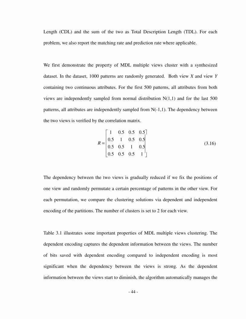
- 44 -
Length (CDL) and the sum of the two as Total Description Length (TDL). For each
problem, we also report the matching rate and prediction rate where applicable.
We first demonstrate the property of MDL multiple views cluster with a synthesized
dataset. In the dataset, 1000 patterns are randomly generated. Both view X and view Y
containing two continuous attributes. For the first 500 patterns, all attributes from both
views are independently sampled from normal distribution N(1,1) and for the last 500
patterns, all attributes are independently sampled from N(-1,1). The dependency between
the two views is verified by the correlation matrix.
=
15.05.05.0
5.015.05.0
5.05.015.0
5.05.05.01
R (3.16)
The dependency between the two views is gradually reduced if we fix the positions of
one view and randomly permutate a certain percentage of patterns in the other view. For
each permutation, we compare the clustering solutions via dependent and independent
encoding of the partitions. The number of clusters is set to 2 for each view.
Table 3.1 illustrates some important properties of MDL multiple views clustering. The
dependent encoding captures the dependent information between the views. The number
of bits saved with dependent encoding compared to independent encoding is most
significant when the dependency between the views is strong. As the dependent
information between the views start to diminish, the algorithm automatically manages the
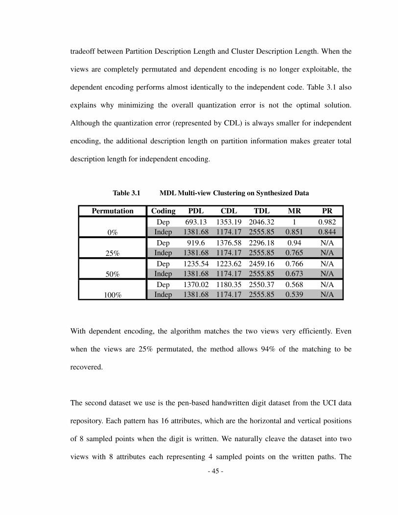
- 45 -
tradeoff between Partition Description Length and Cluster Description Length. When the
views are completely permutated and dependent encoding is no longer exploitable, the
dependent encoding performs almost identically to the independent code. Table 3.1 also
explains why minimizing the overall quantization error is not the optimal solution.
Although the quantization error (represented by CDL) is always smaller for independent
encoding, the additional description length on partition information makes greater total
description length for independent encoding.
Table 3.1 MDL Multi-view Clustering on Synthesized Data
With dependent encoding, the algorithm matches the two views very efficiently. Even
when the views are 25% permutated, the method allows 94% of the matching to be
recovered.
The second dataset we use is the pen-based handwritten digit dataset from the UCI data
repository. Each pattern has 16 attributes, which are the horizontal and vertical positions
of 8 sampled points when the digit is written. We naturally cleave the dataset into two
views with 8 attributes each representing 4 sampled points on the written paths. The
Permutation Coding PDL CDL TDL MR PR
Dep 693.13 1353.19 2046.32 1 0.982
Indep 1381.68 1174.17 2555.85 0.851 0.844
Dep 919.6 1376.58 2296.18 0.94 N/A
Indep 1381.68 1174.17 2555.85 0.765 N/A
Dep 1235.54 1223.62 2459.16 0.766 N/A
Indep 1381.68 1174.17 2555.85 0.673 N/A
Dep 1370.02 1180.35 2550.37 0.568 N/A
Indep 1381.68 1174.17 2555.85 0.539 N/A
0%
25%
50%
100%

- 46 -
externally labeled digit class is not used in the clustering but only used to evaluate the
prediction rate. For clarity and simplicity, we reduce the problem of 10 different digits
into a sub-problem with only 2 different digits. In particular, we are interested in two
pairs, 0-1, 3-8 and 1-7. The 0-1 and 3-8 pairs represent simpler version of the multiple
views clustering problem as both views are significantly different from each other. The 1-
7 pair represents are more difficult problem given the second view (bottom half) of digit
1 and 7 are very similar. By fixing the number of clusters as 2 for both views, the results
are reported in Table 3.2.
Table 3.2 Two View Clustering Results for Different Digit Pairs
Table 3.2 illustrates that the MDL based multiple views clustering algorithm does not
merely minimizes an abstract mathematical function, but have pragmatic implications.
The shorter overall description length leads to better matching rate and prediction rate.
The external class labels are not used in the clustering algorithm. The higher prediction
rate with dependent encoding suggests that the algorithm achieves the cluster partition in
Coding PDL CDL TDL MR PR
Dep 1080.5 25329.8 26410.3 1 0.995
Indep 2139.4 25243.6 27383 0.906 0.985
Coding PDL CDL TDL MR PR
Dep 1079.2 24181.7 25260.9 1 0.795
Indep 1382.3 24443 25825.3 0.562 0.785
Coding PDL CDL TDL MR PR
Dep 996.6 22644.7 23641.3 1 0.988
Indep 1993.5 22513.2 24506.7 0.939 0.981
Digit 0-1
Digit 1-7
Digit 3-8

- 47 -
a more meaningful way by considering the potential dependent information between the
views.
The MDL based multi-view clustering algorithm can also be readily applied to image
segmentation problems. A color image consists thousands or millions of pixels, each
represented by a RGB vector, whose three components correspond to the strength of red,
green and blue. In addition to the color view on the pixels, each pixel also has X-Y
coordination on the X-Y plane, which constitutes the location view of the image. Both
color and position of the pixels are important in finding meaningful segmentation of the
image, but different scales between the two views does not allow combination of two
views into one. The problem is of classical multi-view clustering setting.
Multi-view clustering with pixel color and location view simultaneously can obtain better
segmentation of the picture. Figure 3.1 shows an example of different levels of image
recovery from segmenting image solely based on RGB color and by MDL based multi-
view clustering on a BMP picture, each segments the picture with 10 clusters. For each
pixel, the RGB color of the pixel is replaced by its assigned cluster center RGB color to
show the segmentation. As the multi-view approach uses the spatial information as well
as the color information, it achieves a better recovery of the images.

- 48 -
(a)
(b) (c)
Figure 3.1 MDL Based Multi-View Clustering on Image Segmentation.
(a) is the original image (b) is the MDL based multi-view segmentation (c) is the RGB segmentation

- 49 -
3.5 Model Selection
Until now, we have always assumed the number of clusters are predefined and fixed for
each view in the problem. One trademark property of MDL principle is that it allows
model selection. The description lengths computed from different models are directly
comparable. With this property, we can find a good estimation of the number of clusters
from each view by progressively attempting more complicated models.
The approach is very straightforward: starting with two clusters within each view,
progressively increase the number of clusters. The best number of clusters combination is
the one with the shortest description length. Table 3 demonstrates the method by find the
optimal number of clusters in the digit pair 1-7 problem. The parametric complexity is
approximated with their asymptotic expansion form for the multinomial distributions.
Table 3.3 Selecting Number of Clustering Within Each View
K2=2 K2=3 K2=4
K1=2 25260.9 25124 25068.2
K1=3 25126.5 25062 24955.1
K1=4 25121.3 25052 24961.5
K2=2 K2=3 K2=4
K1=2 8.3 13.8 19.3
K1=3 13.8 22.1 30.3
K1=4 19.3 30.3 41.3
K2=2 K2=3 K2=4
K1=2 25269.2 25137.7 25087.5
K1=3 25140.2 25084.1 24985.4
K1=4 25140.6 25082.3 25002.8
Approximated Parametric Complexity
Total Description Length
Negative Log Likelihood

- 50 -
It is easily identified from Table 3.3 that the number of clusters should be 3 and 4
respectively for the two views in the problem. Although there is possibility some higher
number of clusters might yield even shorter description length, in practice we avoid too
many clusters by imposing an upper bound of the number of clusters for each view.
3.6 Chapter Summary
In this chapter, we have introduced a MDL based multiple view clustering framework. It
adopts a single metric to evaluate the clustering solutions, namely the number of bits to
encode the patterns. This universal metric unifies the partition information with the
cluster variance information, which allows not only automatic information tradeoff
between dependency and quantization error, but also allows the model selection, allowing
the data to inform the number of clusters within each view. Empirical evidence indicates
the MDL multiple views clustering framework captures the dependent information
among the views efficiently, leading to higher matching rate. Also, the cluster solutions
are more informative, supported by higher prediction rate.

- 51 -
4 Semi-Supervised Clustering
4.1 Introduction
Semi-supervised clustering refers to clustering problems where a small percentage of the
patterns are labeled. The situation arises usually because the process of obtaining
abundant labeled data is expensive, if not impossible. As the limited amount of labeled
data is not sufficient to build a model through standard supervised learning, the learner
utilizes the information encompassed in the unlabeled data to improve performance. The
data to be learnt come from set YXD × , where DXx ∈ is a D-dimension vector and Y is
a finite set that represents the partial labels, taking the values from a categorical set
including missing values. Like plain clustering problems, the goal of semi-supervised
clustering is to find the partition mapping from the patterns to a finite set of clusters. In
addition to identifying partitioning structure among the patterns, semi-supervised
clustering also concentrates on building classifier by exploiting the clustering structure
and the restricted numbers of class labels.

- 52 -
There are two common approaches to encompassing the exterior label information in the
clustering paradigm. The first approach is to derive instance-level clustering constraints
from the labels, with patterns sharing the same class label forming must-link constraints
and patterns with different labels forming cannot link constraints, which are enforced in
the clustering process [BBM02][CCM03]. A second approach is to treat the labels as the
consequence of different generating mechanisms from each cluster, building generative
classifiers within each cluster with the available class labels. Homogeneity of exterior
label within a cluster is preferred but not as strictly enforced as in the constrained
clustering approach [GH04]. We concentrate on the second approach in this chapter and
defer discussion on constrained clustering in chapter 5.
In the mixture Gaussian approach to semi-supervised clustering, each pattern is
considered to have a latent variable that represents its cluster assignment. In addition,
each cluster has a multinomial generating mechanism of the class labels. Thus semi-
supervised clustering is also a classifier that each cluster corresponds to a discrete
probability distribution on the class labels. To infer a class label for a pattern, one may
find its most likely cluster assignment first and then find its most likely class label given
the cluster assignment. However, due to the nature of semi-supervised clustering that it
has few labels to offer to the learner, the associated model uncertainty is very significant.
For this reason, Bayesian inference where the class label prediction is made upon all
possible models, rather than the most likely model, is desirable in the semi-supervised
clustering context. This chapter discusses how MDL principle can be applied in building
an optimal Bayes classifier (OBC) for semi-supervised clustering.
- 53 -
4.2 Semi-Supervised Clustering with Mixture
Gaussian Model
The mixture Gaussian model assumes the patterns to be clustered a generated from K
different Gaussian distribution. In generating the patterns, each Gaussian component is
assigned a marginal probability that it is chosen to generate a pattern. The likelihood of a
pattern in the mixture Gaussian model is the weighted sum of the likelihood of all the
components,
( ) ( ) ( )
( )( )
( ) ( )
−Σ−−
Σ=Σ
Σ=Θ ∑=
jj
T
j
j
Djj
K
j
jj
xxxf
xfjfxf
µµπ
µ
µ
2
1exp
2
1,|
,||1
(4.1)
The likelihood for all the patterns is
( ) ( ) ( )∏∑= =
Σ=Θn
i
K
j
jjin xfjfxxxf1 1
21 ,||,...,, µ (4.2)
The probability that a pattern belongs to a particular component is given by the posterior
probability,
( )( ) ( )
( ) ( )∑=
Σ
Σ=
K
j
jji
jji
ij
xfjf
xfjfxf
1
,|
,||
µ
µθ
(4.3)
In semi-supervised clustering, the partial labels are considered in the overall likelihood.
Let ( ) ( ) ( ) nnl yxyxyxD ,,...,,,, 2211= be the labeled data, mnnnl xxxD +++= ,...,, 21 be the
unlabeled data. Assuming that X and Y are conditionally independent given Θ , the
likelihood function for semi-supervised clustering is,

- 54 -
( ) ( ) ( ) ( ) ( ) ( )
Σ
Σ=Θ ∏∑∏ ∑
+
+= == =+
mn
ni
K
j
jji
n
i
K
j
jjijinmn xfjfxfjfyPyyyxxxf1 11 1
2121 ,|,|||,...,,,,...,, µµθ (4.4)
where patterns up to m are labeled and ( )jP θ|. is the probability measure on Y for
component j.
4.3 Posterior Probability and Model Uncertainty
Bayes theorem connects marginal probability, conditional probability and posterior
probability together. In machine learning, Bayes theorem typically takes the following
form,
( ) ( ) ( )( )DP
DPPDP
θθθ
|| = (4.5)
Here, H is a random variable on the set of all considered hypotheses and D is a random
variable on the set of all possible data. ( )θP is the prior probability which represents the
learner’s belief on a given hypothesis before observing the data. ( )θ|DP is the
likelihood of data given the hypothesis. ( )DP is the marginal probability of the data D,
performing as a normalization factor. ( )DP |θ is known as the posterior, the probability
distribution on the set of all considered hypotheses after the learner updates its prior with
the data.
In the learning philosophy of a Bayesian, the learning process corresponds to the update
of the learner’s belief on the hypotheses after seeing the data. The outcome of learning is
a probability distribution on the hypotheses set rather than a single hypothesis. If a single

- 55 -
hypothesis has to be inferred, the maximum a posteriori (MAP) estimation [Deg70] is the
hypothesis that maximizes the posterior probability,
( )( )θθ |maxarg DPHh
MAP∈
= (4.6)
Model uncertainty arises when the posterior distribution is replaced by the MAP
estimation, where the posterior distribution reduces to assigning all probability mass to a
single hypothesis. The amount of model uncertainty depends on the probability density
around the MAP estimator. For example, for three considered hypotheses 321 ,, θθθθ =
and two possible posterior distributions P and Q on the hypotheses that are given by
( ) ( ) ( )
( ) ( ) ( )10
3,
5
2,
10
3
10
1,
5
4,
10
1
321
321
===
===
θθθ
θθθ
QQQ
PPP
Posterior P would have less model uncertainty than Q if the posteriors are replaced by the
MAP estimation because it has a more concentrated probability distribution.
4.4 Bayesian Model Averaging
When the availability of the exterior labels are limited, the uncertainty associated with the
semi-supervised clustering classifier is more significant compared to a classifier built
from fully labeled data. In semi-supervised clustering, the posterior distribution is more
diffused compared to its supervised counter part. Figure 4.1 and Figure 4.2 illustrate a
simple example of learning with half the patterns labeled and with all the patterns labeled
in a mixture Gaussian model, with the posterior learnt from partially labeled data flatter
than the fully labeled data.

- 56 -
0
0.8
1.6
-2
-1.6
-1.2
-0.8
-0.4
0
0
0.005
0.01
0.015
0.02
0.025
0.03
p(u1,u2|D)
u1
u2
Figure 4.1 Posterior of a Mixture Gaussian with 8 Labeled Patterns
0
0.8
1.6-2
-1.6
-1.2
-0.8
-0.4 0
0
0.005
0.01
0.015
0.02
0.025
0.03
p(u1,u2|D)
u1
u2
Figure 4.2 Posterior of a Mixture Gaussian with 4 Labeled and 4 Unlabeled Patterns
Point estimations such as maximum likelihood estimation (MLE) [Ald97] and maximum
a posteriori estimation [Reg70] have reduced performance under considerable model

- 57 -
uncertainties in semi-supervised clustering. The model uncertainty is most well mitigated
by Bayesian model averaging which averages inferences over all possible hypotheses,
weighing each inference by the corresponding posterior probability of the hypothesis. For
a given hypotheses set and prior distribution, Bayesian model averaging achieves the
lowest risk [Mit97]. Mathematically, let Θ be the set of models, Dl be the set of labeled
data and Du be the unlabeled data, the Bayesian model averaging inference uses the entire
posterior distribution for predictive inference. The most probable class label is predicted
as
( ) ( )∫Θ
= θθθ dDDPxyPy uliiyi
,|,|:maxarg (4.7)
This contrasts to the MAP approach that makes predictions from the single model *θ that
has the largest posterior probability.
( ) ( )uliy
DDPxyPi
,|maxarg,,|maxarg ** θθθθ
= (4.8)
We can see that (4.8) approximates (4.7) if ( )ul DDp ,|*θ dominates the posterior
distribution. However, the two predictions can be different if the posterior distribution is
not very peaked, which is typical in semi-supervised clustering. Under this situation, (4.7)
integrates out the parameters to obtain the prediction not conditioned on any particular
model in the model space, as shown in equation (4.9).

- 58 -
( ) ( )
( )( )
( ) ( )( )
( ) ( )( )
( )( )
( ) ( )( ) ( )
( ) ( )( )
( )( )xP
DDxyP
dDDxypDDPxP
dDDPxP
DDxyPP
dDDP
DDP
xP
xyPP
dDDP
DDPP
xP
xyP
dDDPxyP
ul
ul
ul
ul
ul
ul
ul
ul
ul
ul
,|,
,,,,,
1
,
|,,,
,
|,|,
,
|,
,
,,
,|,|
=
=
=
=
=
∫
∫
∫
∫
∫
Θ
Θ
Θ
Θ
Θ
θθ
θθθ
θθθθ
θθθ
θ
θ
θθθ
(4.9)
The main difficulty in performing Bayesian model averaging is to compute the integral
over the posterior distribution ( )ul DDp ,|θ in (4.7). Uniform sampling on Θ typically is
very inefficient way to estimate the integral as most of the samples would have small
posterior probability and thus small weights. Importance sampling [Sri02] is desired to
generate samples from Θ according to the posterior distribution. The integral is
approximated by randomly generating models from the posterior distribution and
averaging the inferences with unity weight. As more probable models are drawn more
often, this approach asymptotically approaches the integral shown (4.7) [GRS96].
Typically it is achieved by constructing a Markov chain on Θ whose stationary
distribution is equivalent to the posterior distribution.

- 59 -
4.5 Markov Chain Monte Carlo (MCMC)
4.5.1 Markov Chain
A Markov chain on set Θ is a collection of random variables tθ that satisfies the
Markov property,
( ) ( )tttt PP θθθθθθ |,...,,| 1101 ++ = (4.10)
The Markov property states that the state of the chain at time t+1 only depends on its
immediate previous state and conditionally independent of its historical path. With this
property, a Markov chain is fully specified by the transition probability ( )ttP θθ |1+ and
the probability on the initial state of the chain ( )0θP . A stationary distribution ( )θπ of a
Markov chain exists if
( ) ( ) ( )11 | +
Θ∈
+ =∑ tttt
t
P θπθπθθθ
(4.11)
A path of Markov chain can be generated by sequentially sampling tθ according to the
transition probability distribution function.
In semi-supervised clustering, the set of model parameters that fully describes the model
is πµω ,,,,, Σ=Θ zk , where k is the number of clusters, ω is the prior probability of each
cluster, z is the vector of cluster assignment for the patterns, Σ,µ describes each of the Gaussian
distributions in the mixture Gaussian model, and π is the parameter that describes the
multinomial distributions on the class labels for each cluster. A state in the Markov chain is a
member of Θ , which is a solution of the semi-supervised clustering problem.

- 60 -
4.5.2 Metropolis-Hastings and Gibbs Algorithm
The Metropolis-Hastings algorithm uses a propose-and-accept method to sample from the
stationary distribution ( ).π by constructing a Markov chain. At each time t, a new state is
proposed by an auxiliary proposal distribution ( ).|.Q . Let Xt =θ , a proposed new state
Yt =+1θ is accepted with probability of
( ) ( ) ( )( ) ( )
=XYQX
YXQYYPaccept
|
|,1minπ
π (4.12)
For symmetrical proposal distribution functions, the probability to accept reduces to,
( ) ( )( )
=X
YYPaccept
π
π,1min (4.13)
If the state is multivariate Mθθθθ ,...,, 21= , a single component Metropolis-Hastings
proposes new states that is only different from the current state by one component. To
update component i, the probability for acceptance of a new state is,
( )( ) ( )( ) ( )
′
′′=′
MiMiMi
MiMiMi
MiacceptQ
QP
θθθθθθθθθπ
θθθθθθθθθπθθθ
,...,,...,|,...,,...,,...,,...,
,...,,...,|,...,,...,,...,,...,,1min,...,,...,
111
111
1 (4.14)
If the proposal distribution is the full conditional distribution,
( )( )
( ) iMi
Mi
MiMid
Qθθθθπ
θθθπθθθθθθ
′′
′=′
∫ ,...,,...,
,...,,...,,...,,...,|,...,,...,
1
1
11 (4.15)
The acceptance probability becomes,
( ) 11,1min,...,,...,1 ==′MiacceptP θθθ (4.16)
In other words, if the new component is proposed from the full conditional distribution,
the Metropolis-Hastings algorithm always accepts the newly proposed state. This
sampling algorithm is known as the Gibbs sampling. A sweep in Gibbs sampler refers to

- 61 -
an iteration of sampling each individual component with the corresponding full
conditional distributions.
4.6 MDL Coupled MCMC
As discussed in chapter 2, an efficient prefix code is equivalent to a probability
distribution. If a description length function can be fully specified as a function of the set
of parameters in semi-supervised clustering model, each full conditional distribution
required in Gibbs sampling can be derived from the description length function. Let L be
such a description length function mapping from the model set Θ to positive real
numbers, the marginal probability of a state is given by the following transformation,
( ) ( )( )MiDMi LP θθθθθθθθ ,...,,...,,exp,...,,...,, 2121 −= (4.17)
The full conditional distribution for the ith parameter is,
( )( )[ ]
( )[ ]∑ −
′−=′
i
MiD
MiD
MiMiL
LP
θ
θθθθ
θθθθθθθθθθθθ
,...,,...,,exp
,...,,...,,exp,...,,...,,|,...,,...,,
21
21
2121 (4.18)
The MDL coupled MCMC sampler is superior to the traditional MCMC sampler in the
following ways
• The MDL coupled sampler allows easier accommodation of exterior class labels. The
label information is readily encompassed in the sampler by creating codes of the labels
within each cluster.

- 62 -
• The MDL coupled MCMC allows jumping across models with different numbers of
components without the need to explicitly specify the prior probability on the
components. Rather, the prior is automatically derived from the parametric complexity
and is consistent with Occam’s razor philosophy.
• When normalized likelihood distribution is used in the encoding, only parameters
which are potentially maximum likelihood estimators need to be considered, essentially
discretizing and reducing the size of the state space.
4.7 Encoding Semi-supervised Clustering with
MDL
We now propose the encoding scheme for probabilistic models in semi-supervised
clustering. The description length formulation for a probabilistic model in semi-
supervised clustering problem includes the following steps.
1. Draw the graphical representation of the probabilistic model that implies our prior
assumption.
2. Encode the model following the links in the graphical representation from root nodes
to leaf nodes, until the observed data are encoded. For labeled data, we encode both
independent attributes x and class label y. For unlabeled data, we only encode
independent attributes x.
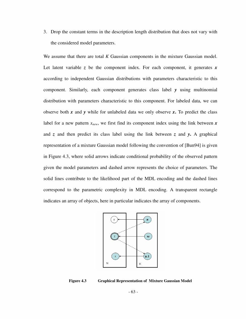
- 63 -
3. Drop the constant terms in the description length distribution that does not vary with
the considered model parameters.
We assume that there are total K Gaussian components in the mixture Gaussian model.
Let latent variable z be the component index. For each component, it generates x
according to independent Gaussian distributions with parameters characteristic to this
component. Similarly, each component generates class label y using multinomial
distribution with parameters characteristic to this component. For labeled data, we can
observe both x and y while for unlabeled data we only observe x. To predict the class
label for a new pattern xnew, we first find its component index using the link between x
and z and then predict its class label using the link between z and y. A graphical
representation of a mixture Gaussian model following the convention of [Bun94] is given
in Figure 4.3, where solid arrows indicate conditional probability of the observed pattern
given the model parameters and dashed arrow represents the choice of parameters. The
solid lines contribute to the likelihood part of the MDL encoding and the dashed lines
correspond to the parametric complexity in MDL encoding. A transparent rectangle
indicates an array of objects, here in particular indicates the array of components.
Figure 4.3 Graphical Representation of Mixture Gaussian Model

- 64 -
The likelihood part to code an unlabeled pattern x is,
( ) ( ) ( ) ( )( )∑=
Σ−−=K
j
jjijiiunlabel xfjzxL1
,|lnln µω (4.19)
The likelihood part to code a labeled pattern (x, y) is,
( ) ( ) ( ) ( ) ( )( )∑=
−Σ−−=K
j
jijjijiiunlabel yfxfjzxL1
|ln,|lnln πµω (4.20)
Three parametric complexities need to be included in the total description length
function: multinomial model to encode the component index, Gaussian model to encode
the unlabeled part of the pattern, multinomial distribution to encode labeled part of the
pattern.
( ) ( ) ( ) ( )NPCNPCNPCNPC KK ,,,, ΠΣΘ ++Ω= (4.21)
The total description length function becomes
( ) ( ) ( ) ( )
( ) ( ) ( ) ( )( )
( ) ( ) ( )( )∑∑
∑∑+
+= =
= =
+
Σ−−
−Σ−−
++Ω=
mn
ni
K
j
jjiji
n
i
K
j
jijjiji
Knmn
xfjz
yfxfjz
NPCNPCNPCyyyxxxL
1 1
1 1
2121
,|lnln
|ln,|lnln
,,,,...,,,,...,,
µω
πµω
ΠΣ
(4.22)

- 65 -
4.8 MDL Coupled MCMC in Semi-Supervised
Clustering
The standard approach to sampling from the posterior distribution is to construct a
Markov chain on the model space that has the posterior distribution as its stationary
distribution. The state of the chain at time t, ,,,,, ttttttt zk πµω Σ=Θ , will only depend
on the state of the chain at time 1−t , ,,,,, 1111111 −−−−−−− Σ=Θ ttttttt zk πµω . The iteration
from time t-1 to t, is a sweep that consists of sampling each parameter conditionally on
all other remaining parameters. In the MDL-MCMC sampler for mixture component
model, there are six moves in each sweep.
1. Sample ω from ( )πµω ,,,,| Σzkf
2. Sample z from ( )πµω ,,,,| Σkzf
3. Death and Re-Birth of a component
4. Split and Combine of a component
5. Sample Σ,µ from ( )πωµ ,,,|, zkf Σ
6. Sample π from ( )Σ,,,,| µωπ zkf
Step 1, 2, 5 and 6 use Gibbs sampling to sample from the full conditional probability
distribution. Step 3 and 4 use Metropolis-Hasting algorithm to handle empty components
and jump across subspaces.
- 66 -
4.8.1 Sample ω
Parameter ω represents the marginal probability of each cluster and must satisfy the
following constraint,
11
=∑=
K
j
jω (4.23)
According to equation (4.22), the description length part that changes with ω is,
( ) ( )( )∑∑+
= =
−=mn
i
K
j
ji jzL1 1
lnωω (4.24)
The challenge in the sampling is to have a proposal function that always satisfies the
unity constraint in (4.23). To fulfil the constraint, we devise the following mapping to
construct the proposal function as illustrated in Figure 4.4,
1. Divide a circle with unity circumference into n+m equally separated segments by
n+m points on the circle.
2. Any combination of K points of the n+m possible on the circle corresponds to a state
of ω . For example, in Figure 4.4, the state is represented as,
DACDBCAB ==== 4321 ,,, ωωωω
3. Starting from the previous state, a new state is proposed by moving each of the K
points one step towards a random direction.
Because the proposal function is symmetrical, the acceptance probability in Metropolis-
Hastings algorithm is simply

- 67 -
( )( )( )
( )( )
−
−=
ω
ωω
L
LP new
newacceptexp
exp,1min
Figure 4.4 Sampling clustering frequency with constraints, K=4, N=8
4.8.2 Sampling z
To sample the latent variable z that represents the cluster assignment of the pattern, we
first write the description length function as a function of z,
( ) ( ) ( ) ( ) ( )( )
( ) ( ) ( )( )∑∑
∑∑+
+= =
= =
Σ−−
−Σ−−=
mn
ni
K
j
jjiji
n
i
K
j
jijjiji
xfjz
yfxfjzzL
1 1
1 1
,|lnln
|ln,|lnln
µω
πµω
(4.25)
Assume the patterns are identically independently distributed (i.i.d.), the sampling is done
with each individual pattern independently. For a labelled pattern,
( ) ( ) ( ) ( )jijjiji yfxfjzL πµω |ln,|lnln −Σ−−== (4.26)
For an unlabled pattern,

- 68 -
( ) ( ) ( )jjiji xfjzL Σ−−== ,|lnln µω (4.27)
For each zi, there are totally K considered alternative encodings, each corresponds to a
different cluster assignment. The probability distribution from which to sample zi is
defined by equation (4.18).
4.8.3 Death and Rebirth
Completely empty components and components that contain only a single pattern require
special attention, as they usually indicate a redundant part of the model that increases the
description length to specify the model yet will not help compress the data. To increase
the mixing rate and shorten the total description length, better parameters can be
proposed to help encode the data. The death and rebirth moves involve destroying an
empty component or a nearly empty component and reinitialize it with new parameters,
which hopefully encode the data more efficiently.
Because an empty component only encodes parametric complexity, the description length
is always the same no matter what the parameters values are. Reinitializing the parameter
values for the empty component does not change the total description length. Also, we
maintain a symmetrical parameter proposal function by reinitialize the parameters
randomly so that the detail balance will be satisfied [Nea93]. If a component contains one
pattern, we cannot always reinitialize the component without a penalty since changes on
the parameters of the component will affect the description length to encode the single
pattern in that component. The increase of the description length is )|(ln newxf θ− since

- 69 -
it takes no description to encode the pattern previously (the pattern will overlap with the
cluster center and the distance from cluster center is zero). Thus the probability of
accepting the move is )|( newxf θ . If the dimensionality of the data is high, then the
acceptance rate becomes very low. One way of overcoming this difficulty is by only
reinitializing the parameter only in one random dimension.
4.8.4 Split and Combine
This is the move that enables sampling across subspaces with different k values. At each
split and combine move, we will stochastically determine whether to attempt to split or to
combine. When k=1, we always attempt the split move and when k equals the maximum
number of components K, we always attempt the combination move. At all other k
values, both the probability to split and the probability to combine are 0.5.
Split. First a random component is chosen as the split candidate. Then we choose the
dimension with the largest standard deviation to generate the split pivot. The split pivot
sp is randomly generated from [ ]σµσµ +− , in the chosen dimension and all patterns
inside the component are divided into two groups: those larger than the pivot and those
smaller in the chosen dimension. All the parameters of the two groups are estimated using
the maximum likelihood estimator. Let j be the candidate component proposed to split
into j1 and j2, the change of the description length after the proposed split can be
calculated from

- 70 -
( ) ( )( )
( )( )( )
( )( )
( )∑∑
∑∑
+
+= =
= =
Σ
Σ+
+
+
Σ
Σ+
=
mn
ni s sjsji
jji
sj
j
i
n
i s sji
ji
sjsji
jji
sj
j
isplit
xf
xfsjz
yf
yf
xf
xfsjzjL
1 2,1 ,,,
1 2,1 ,,,,
,|
,|lnln,
|
|ln
,|
,|lnln,
µ
µ
ω
ω
π
π
µ
µ
ω
ω
(4.28)
The move is subject to a Metropolis-Hasting test and will pass the test with a probability
of ( )( ) jLsplit−exp,1min .
It is also important that the split proposal function and the combination proposal function
be symmetrical. That is, if component j splits into j1 and j2, then the probability of
choosing s for the split attempt should equals the probability of choosing j1 and j2 for the
combination attempt. To achieve this, we enforce that after the split, at least one of the
two newly produced components must be the most adjacent component of the other.
Here, when we say component j1 is the most adjacent component to j2, we mean j1 has
the shortest Euclidean distance to j2. Note that this property is not mutual, that is, j1 is
most adjacent to j2 does not imply that j2 is most adjacent to j1. If none of the two
components is most adjacent to the other, the split attempt is unconditionally rejected. In
later section, we discuss in greater detail in section 4.9 to illustrate that the proposal
function enforces symmetry.
Combine. We pick the two candidate components to combine by choosing the first
candidate component randomly and enforce its most adjacent component as the second
candidate component. The proposed combined component parameters can be easily

- 71 -
estimated from the candidate component’s sufficient statistics. The message length
change for a combination step is the reverse of the split step.
( ) ( )( )
( )( )( )
( )( )
( )∑∑
∑∑
+
+= =
= =
Σ
Σ+
−
+
Σ
Σ+
−=
mn
ni s sjsji
jji
sj
j
i
n
i s sji
ji
sjsji
jji
sj
j
icombine
xf
xfsjz
yf
yf
xf
xfsjzjjL
1 2,1 ,,,
1 2,1 ,,,,
,|
,|lnln,
|
|ln
,|
,|lnln,2,1
µ
µ
ω
ω
π
π
µ
µ
ω
ω
(4.29)
The combination move is evaluated by the Metropolis-Hasting test with an acceptance
probability ( )( ) 2,1exp,1min jjLcombine− . The combination move is the symmetrical move
to the split move. The two moves are reversible and satisfy the detail balancing
equilibrium as we will show in section 4.9.
4.8.5 Sampling µ, Σ
For easy sampling, we assume the covariance matrix Σ is of diagonal form that,
=Σ
2
2
2
2
1
...00
............
0...0
0...0
dσ
σ
σ
(4.30)
It states the attributes of the patterns are independent from one another. The assumption can be
satisfied via rotating the original patterns through principle component analysis (PCA) to make a
new set of attributes that are orthogonal to one another. Once the covariance matrix is diagonal-
ized, the means and variances of each attribute can be sampled independently. The description
length function for the kth Gaussian component and jth attribute is

- 72 -
( ) ( )( )
∑+
=
−++=
mn
i jk
jkji
jkjiji
xmnL
12
,
2
,,
,,,2
ln,σ
µσσµ (4.31)
From the description length function (4.31), jk ,µ can be sampled from a Gaussian distribution
while 2
,
1
jkσ can be sampled from a Chi square distribution.
4.8.6 Sampling π
The description length part that depends on jπ is,
( ) ( )( )∑
=
−=jizi
jij yfL:
|ln ππ (4.32)
The sampling of the multinomial distribution is the same as sampling ω in 4.8.1.
4.9 Convergence
If the stationary distribution of a Markov chain is to converge towards the posterior
distribution, the chain must satisfy the following three conditions [GRS96].
• The chain must be aperiodic, which means there should not be any positive integer, T,
that satisfies ,,,,,,,,,, TtTtTtTtTtTttttttt zkzk ++++++ Σ=Σ πµωπµω for all 0
tt ≥ . If
there is such a T then the chain is periodic and the period of the chain would be T.
• The chain must be irreducible, that is, the transition time takes from any two
states ,,,,, πµω Σzk and ,,,,, πµω ′Σ′′′′′ zk must not be infinity.

- 73 -
• The chain must satisfy the detail balance condition for every move, which is given by
),,,,,,,,,,(),,,,,(
),,,,,,,,,,(),,,,,(
Σ→′Σ′′′′′′Σ′′′′′
=′Σ′′′′′→ΣΣ
µωπµωπµω
πµωµωµω
zkzkpzkp
zkzkpzkp (4.33)
Given any state at time t, the probability the next state is the same state is greater than
zero. Thus it is possible that the chain will stay at one state for arbitrary number of
iterations and move to other states. The chain can only repeat the history with a
probability less than 1. Therefore, the chain can never get into the deterministic cycle that
satisfies the periodicity condition. The chain is also irreducible as the transition
probability between any two states is greater than zero thus it will not take infinite time
for the transition to take place. We now prove that detail balance holds for the six moves.
In the six sampling moves the parameters are sampled from the full conditional
distributions transformed from the message length distribution. In move 1, 2, 5 and 6
where Gibbs sampling is used, it is easy to see the detail balance holds since
( )( ) ( )( ))()(
expexp)()( 122
21211 θθθ
θθθθθ →=
−⋅
−=→ pp
Z
L
Z
Lpp (4.34)
Here θ stands for whichever parameter being sampled in the move and Z is the
normalization factor ( )( )∑ −θ
θLexp .
In move 3 and 4 where Metropolis algorithm is used,
( ) ( ))()(1,min1,min)()( 122211
21
2
12
1
θθθθθθ →===→ −−−
−−−
ppeZ
ee
Z
epp
mmm
mmm
(4.35)
It remains to prove that in the Metropolis test, the proposal function is symmetrical. In
the death and rebirth move, since these parameters are randomly reinitialized, the

- 74 -
probability of a proposal is independent of the current state and is obviously symmetrical.
In the split/combine move, the probability of proposing a component as the split
candidate equals 1/k. The proposed component j is split into j1 and j2. We also enforce
that at least one component resulted from the split must the most adjacent of the other.
Without losing generality, let j2 be the most adjacent component of j1. In the
combination step, the probability of choosing j1 and j2 equals to the sum probability of
choosing j1(which will automatically choose j2 subsequently) and the probability of
choosing j2 and then j1 as its most adjacent component. Let )2,1( jjp be the probability
of proposing components j1 and j2 as the combination candidates and )( jp be the
probability of proposing component j as the split candidate, then
)(11
1
1
1
1)2,1( jp
kkkkjjp ==
++
+= (4.36)
The proposing function is symmetrical and the detail balance holds.
In summary, the proposed MDL coupled MCMC sampler consists of six moves. The
Markov chain grown by the sampler is aperiodic, irreducible and detail balanced
therefore its stationary distribution converges to the MML defined posterior distribution
of the models.
4.10 MCMC Diagnosis
In this section, we empirically diagnose the MDL coupled MCMC sampler to verify the
convergence and analyze the mixing rate. A four component two dimension Gaussian
mixture (Figure 4.5) dataset is used for the purpose. We run the chain for 200,000

- 75 -
iterations with the first 50,000 as the burn-in period. We diagnose the convergence by
comparing the posterior probabilities of k among different segments of the chain, each
with a size of 50,000 iterations. If the chain has converged then the posterior probabilities
should be constant across the segments. The probability of a particular value of k is the
number of iterations the sampler stays in the given model sub-space. The comparison
results are presented in Figure 4.6. Trace plots for k (Figure 4.7) indicates efficient
mixing across the subspaces of different k, with split move and the combine move have
an acceptance rate of 11.2% and 11.3% respectively.
Figure 4.5 Mixture Gaussian Model with Four Components and Two Dimensions

- 76 -
Figure 4.6 Posterior Distribution of k among different time segments in MCMC chain
Figure 4.7 Trace Plot of k (Iteration 180000 to 200000)

- 77 -
4.11 Empirical Results
In this section, we compare the predictive performance between an optimal Bayes
classifier as constructed above and the maximum likelihood classifier usually found by
the EM algorithm. We abbreviate the semi-supervised optimal Bayes classifier as SS-
OBC, and abbreviate the semi-supervised maximum likelihood classifier as SS-EM.
We use standard data sets from the UCI machine learning repository. For each dataset, we
use 10% of the data as labeled data, 10% as the unlabeled data and 80% as the testing
data. We choose small training set size mainly to test the classifiers’ performance when
data is scarce. We report the prediction error and standard deviation over 100 trials. We
also include the p-value of a paired T-test of errors to indicate whether the error reduction
is statistically significant. We summarize our results in Figure 4.1.
Table 4.1 Predictive Performance Comparison between SS-OBC and SS-EM.
*10% labelled data and 10% unlabeled data
We see that for all but one data set that SS-OBC performs significantly better than its SS-
EM rival. Furthermore this improvement in accuracy is often accompanied by a reduction
of the standard deviation of the performance. The reason that SS-OBC showed a non-
statistical significant improvement on the Diabetes dataset is probably that the posterior
Data SS-EM SS-OBC P value
Iris 17.5 (9.9) 10.9(6.9) 6.00E-08
Diabetes 21.2 (7.8) 20.6(6.8) 0.15
Wine 18.1(13.0) 12.4(7.9) 5.20E-05
Glass 56.3 (5.1) 53.7(7.8) 0.0006
Shuttle 21.6 (4.5) 18.6(5.0) 6.50E-08

- 78 -
distribution is already well peaked for the problem even with limited amount of data, thus
an SS-EM can approximate SS-OBC fairly well as the Bayesian integral in equation (4.7)
is dominated by the shortest model.
Next, we gradually decrease the amount of labeled data given to the learner and replace
with unlabeled data. We show the general trend fond for all data sets using Iris, Diabetes
and Wine dataset, as illustrated in Figure 4.8.
We see that in Iris data, an SS-OBC with only 2% labeled data can perform almost as
well as a SS-EM using 10% labeled data. Similarly, in the Wine data, with 4% labeled
data, the SS-OBC classifier achieves comparable prediction accuracy as SS-EM using
10% labeled patterns. This indicates that SS-OBC performs well even when labeled
patterns are very limited, which is an important property in semi-supervised clustering.
In some semi-supervised clustering problems, not only the amount of labeled but also the
amount of unlabeled data is also restricted. In the last experiment, we empirically
investigate the impact of the unlabeled data size on the classifiers. We gradually decrease
the unlabeled data and measure the prediction errors.
Through Figure 4.9, we see that the performance of SS-OBC is superior to that of SS-EM
in semi-supervised learning situations when the unlabeled data as well as the labeled data
is limited. The learner, under this situation, must utilize both labeled and unlabeled data
as efficiently as possible.

- 79 -
Prediction Error of SemiSupervised Learners on Iris
0
5
10
15
20
25
30
35
10% 8% 6% 4% 2%
labeled datap
red
icti
on
err
or
SS-OBC SS-EM
Prediction Error of SemiSupervised Learners on
Diabetes
0
10
20
30
40
50
10% 8% 6% 4% 2%
labeled data
pre
dic
tio
n e
rro
r
SS-OBC SS-EM
Predict ion Error of SemiSupervised Learners on Wine
0
5
10
15
20
25
30
35
40
45
10% 8% 6% 4% 2%
labeled data
pre
dic
tion
err
or
SS-OBC SS-EM
Figure 4.8 SS-OBC and SS-EM on Size of Labele Patterns

- 80 -
Prediction Error w ith Different Amount of Unlabeled
Data for Iris
0
5
10
15
20
25
30
10% 8% 6% 4% 2%
Unlabeled DataP
red
icti
on
Err
or
SS-OBC SS-EM
Predict ion Error with Different Amount of Unlabeled Data for
Diabete
19
20
21
22
23
24
25
26
10% 8% 6% 4% 2%
Unlabeled Data
Pre
dic
tio
n E
rro
r
SS-OBC SS-EM
Prediction Error with Different Amount of Unlabeled
Data for Wine
0.00
5.00
10.00
15.00
20.00
25.00
30.00
10% 8% 6% 4% 2%
Unlabeled Data
Pre
dic
tio
n E
rro
r
SS-OBC SS-EM
Figure 4.9 SS-OBC and SS-EM on Size of Unlabeled Patterns

- 81 -
4.12 Chapter Summary
MDL principle provides description length as the measurement of model complexity
from which we can calculate the posterior probability of the model. In this chapter, we
present procedures to construct optimal Bayes classifiers for probabilistic models in
semi-supervised clustering. The form of the description length calculation can be derived
from the graphical representation of the probabilistic model by encoding the model
parameters and the data in a top-down manner from root to leaf. The description function
implies the full conditional probabilities and can be used to construct a Markov Chain
whose stationary distribution represents the posterior distribution of the model, which
serves as the “weights” used in the optimal Bayes classifier. We verify empirically that
MDL-coupled Optimal Bayes Classifier makes better predictions in semi-supervised
clustering problems compared to the maximum likelihood classifier found by EM in
learning situations where the amount of data is scarce. The semi-supervised optimal
Bayes classifier shows great robustness when very limited amounts of labeled and
unlabeled data are available. This property makes optimal Bayes classifier a very useful
predictor in semi-supervised problems.

- 82 -
5 Constrained Clustering
5.1 Introduction
Clustering algorithm finds partitions for a set of patterns by minimizing dissimilarity
function within clusters. For example, K-means clustering uses squared Euclidean
distance among the patterns for such measure. The found cluster corresponds to implicit
labels. However, in real world problem, it is not immediately clear that these implicit
labels meet the learning purposes. Feedback from expert opinion on the clustering results,
under this scenario, can be beneficial in directing the clustering towards desired learning
goals. Cohn et al. give a Yahoo! Document clustering example [CCM03] where user can
provide feedbacks on clustered patterns advising two patterns belong to the same cluster
or two patterns be exclusive in cluster assignment. The clustering algorithm adopts the
feedback and reconstructs clusters following the constraint added by the user. Constraints
act as background knowledge in learning that help build more meaningful clusters if
handled correctly. The constraints commonly introduced in the clustering context come

- 83 -
into three levels, namely instance-level constraint, cluster-level constraint and model-
level constraint.
Instance-Level Constraint
There are two types of instance-level constraints, known as must-link (ML) and cannot-
link (CL) constraints.
Definition 5.1 (Must-Link Constraint) Let KxP ,...,2,1: → be the cluster
assignment mapping from the pattern space to the cluster indices, pattern xi and xj are
subjective to must-link constraints if ( )( ) ( )( )kxPkxPKk ji =⇔=∈∀ ,...,2,1 .
Definition 5.2 (Cannot-Link Constraint) Let KxP ,...,2,1: → be the cluster
assignment mapping from the pattern space to the cluster indices, pattern xi and xj are
subjective to cannot-link constraints if ( )( ) ( )( ) FkxPkxPKk ji ⇒=∩=∈∀ ,...,2,1 .
The source of the instance-level constraints can be from user feedback as in the Yahoo!
example or be derived from the semi-supervised clustering setting where patterns with
same class labels are imposed must-link constraints and patterns with different class
labels are enforced to be assigned to different clusters. High quality constraints from
expertise opinion can potentially boost the performance of the clustering learner.
Wagstaff et al proposed COP-K-means algorithm [WCR+01] which yields better
performance than plain K-means algorithm by respecting the instance-level constraints
randomly generated from the pattern clusters. Some other algorithm allows violation of
the constraints with an associated penalty [BBM04b].

- 84 -
Cluster-Level Constraint
Davidson and Ravi [DR05] propose two types of cluster-level constraints, named as the
ε-constraint and δ-Constraint.
Definition 5.3 (δ-Constraint) Let KxP ,...,2,1: → be the cluster assignment
mapping from the pattern space to the cluster indices and ( )ji xxD , the distance function,
cluster Ci and Cj are subject to δ-constraint if ( ) ( ) ( ) ( ) TjyPixPyxD ⇒≥== δ,;,min .
Definition 5.4 (ε-Constraint) Let KxP ,...,2,1: → be the cluster assignment
mapping from the pattern space to the cluster indices and ( )ji xxD , the distance function,
cluster Ci is subject to δ-constraint if ( )( ) ( ) ( ) ( )ε≤≠=⇒= xyiyPyxDixP ,;,min .
Cluster-level constraints control the quality of the clusters. δ-Constraint prohibits two
clusters be too similar to each other by specifying the minimal distance allowed between
patterns from two distinctive clusters. ε-Constraint, on the other hand, ensures the
similarity within the same cluster, preventing the distribution of patterns within the same
cluster becoming too loose. The cluster level constraints can be converted into either
conjunctions or disjunctions of the instances-level constraints [DR05].
5.1.1 Model-Level Constraints
In some problems, constraints are put on the maximum size of a cluster to prevent too
small or dominating clusters.

- 85 -
Definition 5.5 (Cluster Size Constraint) Let KxP ,...,2,1: → be the cluster
assignment mapping from the pattern space to the cluster indices and ( )ji,δ be the
disparity function
( )
≠
==
jiif
jiifji
0
1,δ
The clustering model is subject to the cluster size constraint ( )baCSC , if
( )( ) bkxPaKkx
≤≤∈∀ ∑ ,,...,2,1 δ
must hold.
In this chapter, we focus on clustering under the instance-level constraints, as they serve
as building blocks of higher level constraints. We investigate encoding the patterns with
instance-level constraints as background knowledge. The constraints imposed on the
clustering solution essentially induce simpler model by excluding a subset of the solution
space. We show that the simpler model induced by constraints can lead to either shorter
or longer encoding, depending on the expected encoding length on the subset of solution
space. With this philosophy, the encoding length can serve as a yardstick in evaluating the
constraints, thus respect only constraints that facilitate the encoding and ignore the
constraints that result in lengthened codes. We illustrate how good constraints improve
the model performance and bad ones deteriorate the model performance, as well as how
to actively choose good constraints and ignore bad ones within the MDL framework.

- 86 -
5.2 Clustering under Constraints
5.2.1 Feasibility
A fundamental question to ask in constrained clustering is the feasibility of finding
clusters that satisfies the constraints. The question should be answered before any
clustering is attempted in constrained clustering problems where constrains must be
complied. Davidson and Ravi [DR05] investigate the feasibility on various instance-level
and cluster-level constraints. The results indicate that while some constraints such as
must-link constraints are tractable, which means there is a polynomial algorithm in
deciding whether a feasible clustering partition exists, there are intractable constraints
where the feasibility cannot be efficiently decided.
5.2.2 Flexibility
Constraints algorithms fall into two categories. The first type of algorithm faithfully
complies with every constraint specified in the problem, an example of which is the
COP-K-means algorithm. The constraints are said to be hard in this case. Other
algorithms treat the constraints as soft, which can be violated with an associated penalty.
An algorithm enforcing the constraints must subjective to the feasibility problem
mentioned in the previous section. The first level of flexibilities on constraint is whether
a constraint is hard or soft.
Constraints are background knowledge that supposedly augments the performance of the
learner. Indeed, it has been widely reported that learning with constraints, be it hard or

- 87 -
soft, can enhance the learning accuracies [WCR+01] [BBM04a] [GH04] [GVG05].
However, recently research indicates that constraints can potentially have adverse effects.
For example, enforcing a must-link constraint between two patterns with large distance is
likely to weaken the clustering quality. There are two approaches to addressing the issue.
The first solution is to trust the constraints and learn the distance function to
accommodate the constraints [DWB06] [BBM04c]. Alternatively, one can trust the
distance function and evaluate on the constraints. Davidson et al. proposed
informativeness and coherence measures on constraints, enabling the learning to identify
constraints with adverse effects and ignore them [DWB06]. The second level of
flexibility in constraints is whether a constraint is beneficial or harmful.
In the scope of this work, we adopt the second approach: the learner is being faithful to
using description length as universal metric measuring model quality, with which the
constraints are evaluated.
5.3 Constraints and Codes
Previous chapters have already introduced the MDL code to encode patterns with
clustering models without loss of information in unconstrained clustering. In constrained
clustering, the constraints are considered as background knowledge or prior knowledge
shared by the sender and receiver of the code. Depending on the relevance of the prior
knowledge, the code in constrained clustering may or may not be shorter compared to its
unconstrained counterpart. This essentially provide a yardstick in evaluating constraint
qualities and allows flexible usage of the constraints: a constraint is considered to be

- 88 -
beneficial if the total code length is reduced and should be respected; on the other hand, a
constraint can be decided as detrimental to the model if the code length is augmented by
incorporating the prior knowledge and such constraints should be ignored.
As discussed in chapter 2, the description length costs breaks into two parts in encoding
the patterns with clustering models. First the cluster assignment has to be encoded for
each pattern. Then the distance between the pattern and assigned cluster center is
encoded. In constrained clustering, there are less partition solutions than the
corresponding unconstrained problem. From the perspective of coding, the constrained
clustering model is a simpler model that the unconstrained counterpart. The constraints
define a subset of the models from the unconstrained model space and reduce the
parametric complexity of the model. However, the total encoding length may increase if
such model simplification leads to poor data fitting.
Definition 5.6 (Description Length Density) For probability measure f on set P,
the description length density of f on PQ ⊆ is defined as,
( )
( ) ( )
( )∫
∫−
=
Q
Q
f
dxxf
dxxfxf
QDLD
ln
(5.1)
The description length density measures the average encoding length within a subset. A
large description length density on a subset indicates encoding the events within the
subset is not efficient and vice versa. In constrained clustering, the subset of events
excluded by the constraints need to be of high description length density in order to
results in shorter encoding if constraints are used.

- 89 -
Theorem 5.1 Let P be the set of possible partition events for unconstrained clustering
and Q be the set of partition events of constrained clustering. Let ω be the probability
measure on P that corresponds to the efficient prefix MDL encoding. If
( ) ( )QPDLDQDLD −≤ ωω
Then encoding with constraints results in shorter expected description length.
Proof: The expected description length for the non-constraint clustering is given by,
( )[ ] ( ) ( )dppppELP
PNC ∫−=−= ωωω lnln (5.2)
After the events set is reduced from P to Q, the prefix code is renormalized, the new
probability density on Q becomes,
( ) ( )( )∫
=
Q
q
ω
ωψ
(5.3)
The expected description length for the constrained clustering is
( )[ ] ( ) ( ) ( )( )
( )( )
( ) ( )
( )( )∫
∫
∫
∫∫∫
∫
+−=
−=−=−=
Q
Q
Q
Q
Q
QCC
dppdpp
dqqq
dqdpp
q
dpp
qdqqqqEL
ωω
ωω
ω
ω
ω
ωψψψ
ln
ln
lnlnln
The change of the expected description length is given by,

- 90 -
( ) ( )
( )( ) ( ) ( )dpppdpp
dpp
dqqq
LLLPQ
Q
Q
NCCC ∫∫∫
∫++−=−=Λ ωωω
ω
ωω
lnln
ln
Let ( )
αω
+=
∫1
1
dppQ
( ) ( ) ( ) ( ) ( ) ( ) ( ) ( )
( ) ( ) ( ) ( ) ( )
( )
( ) ( )
( ) ( )
( ) ( )
( )( )
( )
( ) ( )
( )
( ) ( )
( )( )
( ) ( )( ) ( ) ( )
0
ln
ln
lnln
ln
ln
11
ln
lnlnln
lnlnlnln1
≤
+−−=
+
−=
+
−−=
+−=
++++−=
−=∆
∫∫
∫∫
∫
∫
∫∫
∫∫
∫
∫∫
∫∫
∫∫∫
∫∫∫∫
−
−
−
−
−−
−
−
−
−
QQP
Q
Q
Q
QP
QP
QP
Q
QP
Q
QQP
QP
QP
QQQP
QQPQQ
NCCC
dppdppQPDSDQDSD
dppdpp
dqqq
dpp
dppp
dpp
dppdpp
dqqq
dppdpp
dppp
dpp
dppdqqqdppp
dpppdpppdppdqqq
LLL
ωω
ωω
ωω
ω
ωω
ω
ωω
ωω
ωω
ωω
ω
ωωωαωω
ωωωωωωωα
ωω
Q.E.D.
Theorem 5.1 states that the learner expects to encode with shortened description length if
the subset of events which has been removed by the constraints have a higher description
length density than the subset of events that are compatible with the constraints. A
constraint is “sound” if it decreased the expected description length by removing the
lengthy encoding subsets from the entire set of events.
Theorem 5.2 ( ) ( ) ( ) ( )QDLDPDLDQDLDQPDLD ωωωω ≥⇔≥−
- 91 -
Proof: The proof is straightforward,
( ) ( )∫=Q
dqqQW ω
By the definition of description length density,
( ) ( ) ( ) ( ) ( )PDSDQPDSDQPWQDSDQW ωωω =−−+
( )( )
( ) ( ) ( )( ) ( )
( )( )
( )
( )QPW
QWQDSD
PDLD
QDLDQPW
QDSDQWPDLD
QDLD
QPDLD
−
−
=−
−=
− ω
ω
ω
ωω
ω
ω
Since ( ) ( ) 1=−+ QPWQW
( )( )
( )( )
11 ≥⇔≥−
QDSD
PDLD
QDLD
QPDLD
ω
ω
ω
ω
Q.E.D.
Theorem 5.2 together with 5.1 states that it is sufficient to compare the description length
density of the unconstrained event set with that of the constrained event set to decide the
soundness of a constraint.
5.4 MDL Clustering with Instance-Level Con-
straints
5.4.1 Encoding Must-Link Constraints
We view constraints are prior knowledge or agreements on codes shared by the sender
and receiver. For example, if pattern ix and jx form a must-link constraint, the sender

- 92 -
can encode the clustering assignment information of the two patterns together. The
receiver, on the other hand, should expect such encoding and knows that the cluster
assignment would not be encoded redundantly once the cluster assignment information of
ix is assigned.
The must-link constraints have following entailment property,
( ) ( ) ( )kikjji xxMLxxMLxxML ,,, ⇒∩ (5.4)
Such property allows identifying must-link pattern sets within which patterns must make
the same clustering assignments. Must-link constraints allow economical coding on
clustering assignments, but the same inflexibility may lead to larger encoding costs on the
disparities between the pattern and cluster center.
.
The must-link subsets are identified by searching for the connected components in an
auxiliary graph G(V,E) in the following steps.
1. The set of vertices V form a one-to-one mapping to the set of patterns
2. Connect undirected edge ( )ji vvE , if ( )
ji xxML ,
3. Find the set of connected components of G by breadth first search algorithm
We use a flag iCCf to indicate if a connected component is already encoded. The flag does
not have to be part of the description that the sender sends to the receiver. It is only used
in constructing the code. The receiver can construct the flags unambiguously from the
constraints when decoding the message. The steps to construct the code for the cluster
assignment information with the auxiliary graph are,
1. Initialize the encoding flag for each connected component as 0

- 93 -
2. For each pattern ix , identify its connected component.
3. If the flag of the connected component is 0, then encode the cluster assignment of the
pattern and set the encoding flag of the connected component to 1. If the flag of the
connected component is 1, then no encoding is needed for cluster assignment of ix .
4. Encode the distances of each pattern from its assigned cluster center.
Example 5.1 (Must-Link Encoding) Let 9.0,8.0,5.0,2.0,1.0 54321 ===== xxxxx be
five patterns to be clustered into three clusters. The must-link constraints are
( ) ( )5421 ,,, xxMLxxML . A feasible partition is 54321 ,,, xxxxx . Further, the prefix code
to encode the cluster assignment corresponds to probability measure P such that
( ) ( )5
22,
5
31 == PP
The encoding of the patterns can be accomplished with the following steps,
1. A Breadth-First search identifies the connected components are 54321 ,, xxxxx .
2. Encode 1x with description length ( )1ln P− and set flag 11
=CCf , which is indicated
by Figure 5.1 (b).
3. When encode 2x , the sender check that 12 CCx ∈ and 11
=CCf . Thus no encoding is
needed for 2x . The receiver of the code can determine the cluster assignment of 2x
from the constraints and earlier part of the code.
4. 3x is encoded with description length of ( )1ln P− and set flag 12
=CCf .
5. 4x and 5x are encoded similarly as 1x and 2x using the must-link constraint.

- 94 -
6. The distances of the patterns from the assigned clusters are encoded with equation
(2.29).
(a) (b) (c) (d)
Figure 5.1 Encoding with Must-Link Constraints in Example 5.1
5.4.2 Encoding Cannot-Link Constraints
Because cannot-link constraints do not have the entailment property as must-link
constraints, the encoding is more complicated. As mentioned previously, the feasibility
problem for cannot-link constraints is NP-complete. Thus there is no known polynomial
algorithm to decide if a code exists to encode the patterns while fulfilling the constraints.
However, assuming that a feasible clustering solution has already been found, the
patterns can be encoded with the following steps,
1. Construct an auxiliary graph for the cannot-link constraints similarly as in the must-
link constraints.
2. For each pattern ix , initialize coding flag as 0.
3. For each pattern ix , if all adjacent vertices in the auxiliary graph have coding flag 0,
encode the cluster assignment with the same prefix code as unconstrained clustering
and change coding flag to 1. If some adjacent vertices in the auxiliary graphs have

- 95 -
coding flag 1, code cluster assignment by renormalizing the unconstrained code and
change coding flag to 1.
4. Encode the distances of each pattern from its assigned cluster center.
Example 5.2 (Cannot-Link Encoding) Let 9.0,8.0,5.0,2.0,1.0 54321 ===== xxxxx
be five patterns to be clustered into three clusters. The cannot-link constraints are
( ) ( )5331 ,,, xxCLxxCL . A feasible partition is 54321 ,, xxxxx . Further, the prefix code
to encode the cluster assignment corresponds to probability measure P such that
( ) ( ) ( )5
23,
5
12,
5
21 === PPP
To encode the cluster assignments of the patterns, we first construct the auxiliary graph,
Figure 5.2 Cannot-Link Encoding Auxiliary Graph for Example 5.2
The encoding of the patterns are done sequentially with inference to the auxiliary graph G
in Figure 5.2,
1. 1x is encoded with description length ( )1ln P− .
2. 2x is encoded with description length ( )1ln P− .

- 96 -
3. In encoding 3x , the sender checks the neighboring vertices in the auxiliary graph G
and found 1x is already encoded to be assigned to cluster 1. 3x can only be assigned
to either cluster 2 or 3. Thus prefix code P becomes redundant by reserving code to
encode the event of assigning 3x to cluster 1. The probability measure P is
renormalized into Q by excluding events that conflicts the cannot-link constraint.
( ) ( )3
23,
3
12 == QQ
The description length to encode the cluster assignment of 3x to cluster 2 is
( )2ln Q− . The description length saved is ( ) ( )3
5ln2ln2ln =− PQ .
4. 4x is encoded with description length ( )3ln P− .
5. 5x is encoded in the similar way as 3x , by excluding the event of assigning 5x to
cluster 2, the probability measure is renormalized into
( ) ( )2
13,
2
12 == QQ
The description length saved is ( ) ( )4
5ln3ln3ln =− PQ
6. The distances of the patterns from the assigned cluster centers are encoded with code
in equation (2.29).
5.4.3 Optimization
The optimization is done in a similar fashion to K-means clustering, while replacing the
quantization error with description length cost. Within each iteration, a pattern is assigned
to the cluster that offers shortest encoding of the pattern while maintaining the integrity
- 97 -
of the constraints. The encoding cost of the patterns can be represented by an encoding
cost matrix C, where each row represents a pattern and each column a potential cluster
assignment of the pattern. [ ]jiC , entry represents the encoding cost associated with
assigning pattern i to cluster j. To minimize the total encoding cost, the cluster
assignment for each pattern is simply,
( ) [ ]jiCxPj
i ,minarg= (5.5)
The minimization is less straightforward when it subjects to a number of must-link and
cannot-link constraints. Again, the problem is NP-complete in nature and we cannot hope
to find an exact solution. Instead, we assume the constraints form an easy set [DR06]
where iterative algorithms will converge to a feasible solution.
The cannot-link constraints may potentially enforce the learner to make a cluster
assignment that is not the shortest description length in the row of the coding matrix
representing a pattern. The worst case scenario is the clustering assignment associated
with the longest description length has to be chosen due to constraints. We define
maximum coding risk (MCR) as the largest possible extra encoding cost of a constrained
assignment versus when the assignment is unconstrained for a given pattern,
[ ]( ) [ ]( ) [ ]( ),.min,.max,. iCiCiCMCR −= (5.6)
Within the scope of respecting the constraints, the learner should prefer to make
assignment for patterns with larger MCR first.
In [DR06], Davidson and Ravi proposed an algorithm that generates the inductive
ordering of the patterns to achieve convergence for a clustering problem with easy

- 98 -
constraints set. Here, we modify the algorithm slightly to accommodate our need to
minimize the description length within the scope of satisfying the constraints.
1. Generate connected components with breadth-first search.
2. Generate auxiliary graph G (V, E) with each node corresponding to a connected
component and each edge corresponding to a cannot-link constraint.
3. E-Step
a. Generate encoding cost matrix C.
[ ] ∑∈
−+−=
iCCx j
j
j
xjiC
2
2
ln,σ
µω
b. Generate Q-inductive Order icc
While Φ≠V
i. Find a node Vv ∈ with minimum degree. For nodes with the same
number of degrees, find the node with smallest MCR defined in
(5.6)
ii. Insert v at the head of the list L
iii. vVV −=
End While
c. For each icc , set constraint list ( ) Φ=iccCList
d. For each Lcci ∈ from head to tail

- 99 -
i. ( )( )
[ ]jiCccziCListj
i ,minarg∉
=
ii. For each kcc that ( ) 1, =ik ccccE
( ) ( ) ( )ikk cczccCListccCList ∪=
4. M-Step
a.
( )( )
N
jxzN
i
i
j
∑== 1
,δ
ω
b.
( )( )
( )( )∑
∑
=
==N
i
i
N
i
ii
j
jxz
xjxz
1
1
,
,
δ
δ
µ
c.
( )( )
( )( )∑
∑
=
=
−
=N
i
i
N
i
jii
j
jxz
xjxz
1
1
2
2
,
,
δ
µδ
σ
5. Repeat step 3 and 4 until the solution converges.
5.5 Constraints Violation
Not all constraints are beneficial to the clustering process. Poorly specified constraints
such as must-link constraints among very disparate patterns give rises to clusters with
large within-cluster dissimilarities. For example, the feedback in the Yahoo! example is
not guaranteed to be of high quality as anyone can potentially provide any constraints. It
- 100 -
is essentially important to evaluate constraint quality and ignore poorly specified
constraints.
Theorem 5.1 and 5.2 provides a method in determining the quality of the constraints.
Constraints, as background knowledge in the clustering problem, should supposedly
shorten the overall description length. Any imposed constraints that necessarily increase
the encoding cost should be ignored if the constraints are not enforced to be hard, as the
choice between encoding with constraints and without is essentially a model selection
problem and the description length of the pattern is the ubiquitous metric that decides the
outcome of the model selection.
The algorithm in the previous section can be readily modified to accommodate the
constraint evaluation mechanism implied by theorem 5.1 and 5.2 in the E-Step, when the
patterns are assigned to clusters by evaluating the encoding costs associated with each of
the clusters. The expected encoding cost with the constraints can be compared to that
without, and the learner only enforces a constraint if it allows shortening of the
description. To address the decoding issue, the code reserves a single bit as a flag to
indicate if a constraint is enforced so that the receiver can decipher the code accordingly.
5.6 Empirical Results
In this section, we use UCI dataset to empirically validate the MDL based instance-level
constrained clustering approach proposed in the chapter. All datasets have continuous
attributes, which are standardized. Each dataset is randomly divided into training set
- 101 -
(80%) and test set (20%). Within the training set, must-link constraints and cannot-link
constraints are generated with different constraint percentages (CP) from the class labels.
A derivation of the algorithm outline in 5.5 by incorporating the encoding cost of the
class labels is used to find the cluster solutions. Each cluster is associated with a class
label by majority counting. This allows classification of the patterns in the test set with
two steps: first assign a pattern to a cluster (there is no constraint in the test set) and then
the predicted label is the one that corresponds to the assigned cluster. The reported
accuracy is an average over 10 runs.
In the first experiment, all constraints are faithfully generated from the class labels. For
patterns with the same class label, we assign must-link constraints and for patterns with
different class labels, we assign must-link constraints. The empirical results are indicated
in Figure 5.1. With increased percentage of constraints, both the accuracy of the training
set and testing set improves steadily, indicating that the constraints derived from the class
labels have influenced the cluster solutions towards befitting the purpose of predicting the
class labels. It also suggests that class labels can provide more information than passively
serving as associating clusters with classes by simple majority counting, they can actively
participate in the clustering solution search process and thus boost the overall
performance.

- 102 -
Figure 5.3 Performance of UCI Datasets from Different Percentage of Constraints Generated
from Class Labels
The second experiment is similar to the first one, except that the constraints are generated
purely randomly, independent of the class labels. Such constraints with no insights should
be detrimental to the learner and lengthens the encoding cost if the constraints are to be
enforced. The results are shown in Figure 5.4, where both the training and testing sets
have impaired performance when more randomly generated constraints are introduced. It
shows poorly specified constraints can deteriorates the clustering solution significantly.

- 103 -
Figure 5.4 Performance of UCI Datasets from Different Percentage of Constraints Generated
Randomly
In the third experiment, 60% of the generated constraints are from class labels and 40%
are generated randomly. We compare the results between “soft constraints”, which allow
MDL actively choosing “sound” constraints that lead to shortened description length, and
“hard constraints”, where the clustering results are partially dictated by the constraints.
Empirical results show that MDL can evaluate the quality of the constraints correctly and
improves the performance of the training set. However, empirical results indicate that
even without actively choosing the “good” constraints, the performance of the testing set
is resistant to the certain percentage of bad constraints. A possible reason is that the “bad”
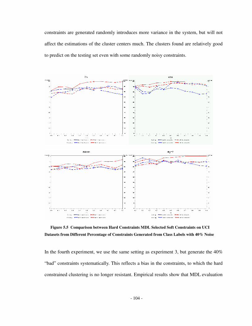
- 104 -
constraints are generated randomly introduces more variance in the system, but will not
affect the estimations of the cluster centers much. The clusters found are relatively good
to predict on the testing set even with some randomly noisy constraints.
Figure 5.5 Comparison between Hard Constraints MDL Selected Soft Constraints on UCI
Datasets from Different Percentage of Constraints Generated from Class Labels with 40% Noise
In the fourth experiment, we use the same setting as experiment 3, but generate the 40%
“bad” constraints systematically. This reflects a bias in the constraints, to which the hard
constrained clustering is no longer resistant. Empirical results show that MDL evaluation

- 105 -
of the constraints actively choosing the good constraints and yield significantly better
accuracies than if all the constraints are faithfully respected.
Figure 5.6 Comparison between Hard Constraints MDL Selected Soft Constraints on UCI
Datasets from Different Percentage of Constraints Generated from Class Labels with 40% Bias
5.7 Chapter Summary
In constrained clustering, the cluster partition solution is subject to a set of must-link and
cannot-link constraints which are generated either from expert opinion or class labels.
While well specified constraints increase the performance of the learner, poorly defined
constraints can mitigate the learning quality. In this chapter, we propose the MDL

- 106 -
approach to solving the constrained clustering problem, which allows active
identification of randomly bad constraints due to variance and systematically bad
constraints due to bias. The empirical results indicate that the method performs well in
both cases by ignoring the bad constraints. In particular, it is most useful in identifying
bad constraints due to bias to which the performance of a learner is most vulnerable.

- 107 -
6 Conclusion and Future Work
This thesis explores three informed clustering problems by utilizing minimum description
length principle. Within the established MDL informed clustering framework, various
information are all encoded into binary strings and information amount is measured
ubiquitously by the string lengths. This allows straightforwardly managing the trade-off
among information of various types. In particular, for each type of informed clustering
problem, the thesis describes the following aspects:
• How to encode patterns within the clustering context. This includes encoding pattern
assignments to clusters and the disparities between patterns and cluster centers. In
addition, in multi-view clustering, the thesis proposes the joint encoding of the views;
in semi-supervised clustering, the thesis describes the encoding of the partial labels; in
constrained clustering, the thesis discusses encoding with constraints as background
knowledge.

- 108 -
• How to search for the shortest code. The thesis uses EM optimization algorithm when
model uncertainty is less significant such as in multi-view clustering and constrained
clustering. While in semi-supervised clustering where the limited partial label induces
significant model uncertainty, the thesis proposes a MDL based Markov Chain Monte
Carlo sampler, which allows efficient sampling of the posterior distribution and
constructing the Optimal Bayes Classifier (OBC).
• How to decide the model selection problem. A major advantage of the MDL based
informed clustering framework proposed in the thesis is that model selection problem
can be conveniently addressed within the framework. As MDL considers both model
complexity and goodness of data fitting, models of different complexity can be directly
compared using the encoding length as the yardstick. In multi-view clustering, the
framework allows model selection between modelling the views as independent and as
dependent; in semi-supervised clustering, it allows automatic jumping across mixture
Gaussian model space with different number of components; in constrained clustering,
it allows the learner to judge the soundness of the constraints, thus exploiting the
beneficial constraints and ignores the detrimental ones.
Empirical results indicated that the MDL based inference yields improved performances
in various informed clustering problems. The framework proposed in the thesis avail
itself as a learning flexible tool to handle various types of background information in
informed clustering problems and make inferences that are immune to model over-fitting
or under-fitting.

- 109 -
Future Research Directions
The thesis is the first attempt in establishing a unified framework among various types of
informed clustering problems. The thesis explores to certain level of details of the
encoding of various types of background information, but it requires further
supplementation and refinement at least in the following aspects:
• In multi-view clustering, when the number of views increases from two, the algorithm
proposed in chapter 3 has an exponential computational complexity to the number of
views. Automatic selecting the most informative views from large number views of the
data is a challenging problem.
• In semi-supervised clustering, a very simple multinomial model is built within each
cluster in predicting class labels. In principle, any classifier can be combined with
clustering to give rise to local classifier for each cluster, known as the divide and
conquer approach. Incorporating other classifiers into the semi-supervised clustering
can potentially further improve the model performance.
• In constrained clustering, the thesis explored encoding with instance-level constraints.
To have a complete framework, further research is needed for encoding under cluster-
level constraints and model-level constraints.

- 110 -
References
[Ald97] Aldrich, J., R.A. Fisher and the making of maximum likelihood,. Statistical
Science 12 (3): 162-176, 1997.
[BBM02] Basu, S., Banerjee, A., Mooney, R.J., Semi-supervised clustering by seeding,
Proceedings of the Nineteenth International Conference on Machine Learning,
2002.
[BBM04a] Basu, S., Bilenko, M. and Mooney, R.J., A probability framework for semi-
supervised clustering, Proceedings of the tenth ACM SIGKDD international
conference on Knowledge Discover and Data Mining, 2004.
[BBM04b] Basu, S., Banerjee, A. and Mooney, R.J., Active semi-supervision for pairwise
constrained clustering, Proceedings of the 2004 SIAM International Conference
on Data Mining, 2004.
[BBM04c] Bilenko, M., Basu, S. and Mooney, R.J., Integrating constraints and metric
learning in semi-supervised clustering, Proceedings of the twenty-first
international conference on Machine learning, 2004.
[BM98] Blum, A. and Mitchell T., Combining labeled and unlabeled data with co-
training, Proceedings of the eleventh annual conference on Computational
learning theory, 1998.
[BO00] Baxter, R.A. and Oliver J.J, Finding overlapping components with MML.
Statistics and Computing, 10, 1, 2000.

- 111 -
[BS04] Bickel, S., Scheffer and T., Multi-View Clustering, Proceedings of the IEEE
International Conference on Data Mining, 2004.
[Bun94] Buntine, Operations for Learning with Graphical Models, Journal of Artificial
Intelligence Research, 1994.
[CCM03] Cohn, D., Caruana, R. and McCallum A., Semi-supervised Clustering with User
Feedback. Technical Report TR2003-1892, Cornell University, 2003.
[Dav00] Davidson, I., Minimum Message Length Clustering Using Gibbs Sampling,
Proceedings of the sixteenth International Conference on Uncertainty in Artificial
Intelligence, 2000.
[Deg70] DeGroot, M, Optimal Statistical Decisions, McGraw-Hill, 1970.
[DR05] Davidson I. and Ravi, S.S., Clustering under Constraints: Feasibility Issues and
the K-Means Algorithm. Proceedings of the fifth SIAM International Conference
on Data Mining, 2005.
[DR06] Davidson I., Ravi S.S., Identifying and Generating Easy Sets of Constraints For
Clustering, Proceedings of the twenty-first National Conference on Artificial
Intelligence, 2006.
[DWB06] Davidson I., Wagstaff, K. and Basu, S., Measuring Constraint-Set Utility for
Partitional Clustering Algorithms , Proceedings of the tenth European Conference
on Principles and Practice of Knowledge Discovery in Databases, 2006.
[FAD00] Fitzgibbon, L.J., Allison, A. and Dowe, D.L., Minimum Message Length
Grouping of Ordered Data, Algorithmic Learning Theory, the eleventh
International Conference on Algorithmic Learning Theory, 2000.

- 112 -
[GH04] Gondek, D. and Hofmann, T., Non-Redundant Data Clustering. Proceedings of
the fourth IEEE International Conference on Data Mining (ICDM), 2004.
[GRS96] Gilks, W., Richardson, S. and Spiegelhalter D., Markov Chain Monte Carlo in
Practice. Interdisciplinary Statistics. Chapman and Hall, 1996.
[GVG05] Gondek, D., Vaithyanathan, S. and Garg A., Clustering with Model-level
Constraints, Proceedings of the 2005 SIAM International Conference on Data
Mining, 2005.
[Har75] Hartigan, J.A., Clustering Algorithms, John Wiley & Sons, Inc. New York, NY,
USA, 1975.
[JD88] Jain, A.K. and Dubes, R.C., Algorithms for clustering data, Prentice-Hall, Inc.
Upper Saddle River, NJ, USA, 1988.
[JMF99] Jain A.K., Murty M.N. and Flynn, P.J., Data Clustering: A Review, ACM
Computing Surveys (CSUR), 1999.
[Jol86] Jolliffe, I.T., Principal Component Analysis. Springer-Verlag, 1986."
[KGV83] Kirkpatrick, S, Gelatt, C. D. and Vecchi, M. P., Optimization by Simulated
Annealing, Science, Vol 220, Number 4598, pages 671-680, 1983.
[KMB+03] Kontkanen, P., Buntine, W., Myllymaki, P., Rissanen, J. and Tirri, H., Efficient
computation of stochastic complexity, the Ninth International Workshop on
Artificial Intelligence and Statistics, 2003.

- 113 -
[KMB+05] Kontkanen, P., Myllymaki, P., Buntine, W., Rissanen, J. and Tirri, H., An MDL
framework for data clustering, Advances in Minimum Description Length:
Theory and Applications, 2005.
[KNS+05] Kaski, S. Nikkila, J. Sinkkonen, J. Lahti, L. Knuuttila, J.E.A. and Roos, C.,
Associative clustering for exploring dependencies between functional genomics
data sets, IEEE/ACM Transactions on Computational Biology and
Bioinformatics, 2005.
[Mit97] Mitchell, T., Machine Learning, McGraw Hill, 1997.
[MRA95] Mehta, M., Rissanen, J. and Agrawal, R., MDL-based decision tree, Proceedings
of the first International Conference on Knowledge Discovery and Data Mining,
1995.
[Nea93] Neal, R., Probabilistic Inference Using Markov Chain Monte Carlo Method,
Technical Report CRG-TR-93-1, Department of Computer Science University of
Toronto, 1993."
[QR89] Quinlan, J.R. and Rivest, R.L., Inferring decision trees using the minimum
description length principle, Information and Computation, 1989.
[Ris01] Rissanen, J., Strong optimality of the normalized ML models as universal codes
and information in data. IEEE Trans. Information Theory, 47, 5, 2001.
[Ris78] Rissanen, J., Modeling by shortest data description. Automatica, vol. 14 1978.
[Ris87] Rissanen, J., Stochastic complexity. The Journal of the Royal Statistical Society,
Series B, Methodology, 49, 3, 1987.

- 114 -
[Ris96] Rissanen, J., Fisher information and stochastic complexity. IEEE Trans.
Information Theory, vol. 42, pp. 40-47, 1996.
[Sri02] Srinivasan, R., Importance sampling - Applications in communications and
detection, Springer-Verlag, Berlin, 2002.
[WB68] Wallace, C.S. and Boulton, D.M., An information measure for , Computer
Journal, 1968.
[WCR+01] Wagstaff, K., Cardie, C., Rogers, S. and Schrödl, S., Constrained K-means
Clustering with Background Knowledge. Proceedings of the Eighteenth
International Conference on Machine Learning, p.577-584, June 28-July 01,
2001.
[WF87] Wallace, C.S., Freeman, P.R., Estimation and Inference by Compact Coding. The
Journal of the Royal Statistical Society, Series B, Methodology, 49, 3, 1987."
[WP93] Wallace, C.S. and Patrick, J.D., Coding Decision Trees, Machine Learning, 1993.