INFERENTIAL STATISTICS PRESENTATION

MBA-13 BATCH 1

CREATED BY: SAJIDA PARVEEN

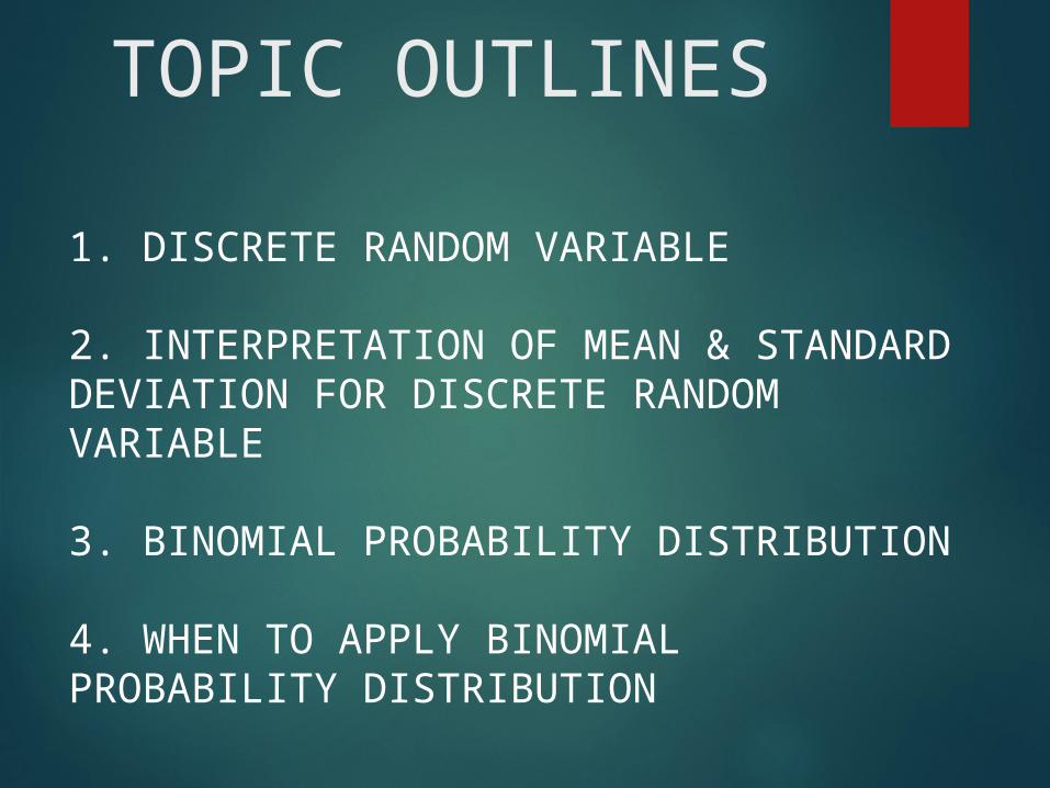
TOPIC OUTLINES

1. DISCRETE RANDOM VARIABLE

2. INTERPRETATION OF MEAN & STANDARD DEVIATION FOR DISCRETE RANDOM VARIABLE

3. BINOMIAL PROBABILITY DISTRIBUTION

4. WHEN TO APPLY BINOMIAL PROBABILITY DISTRIBUTION

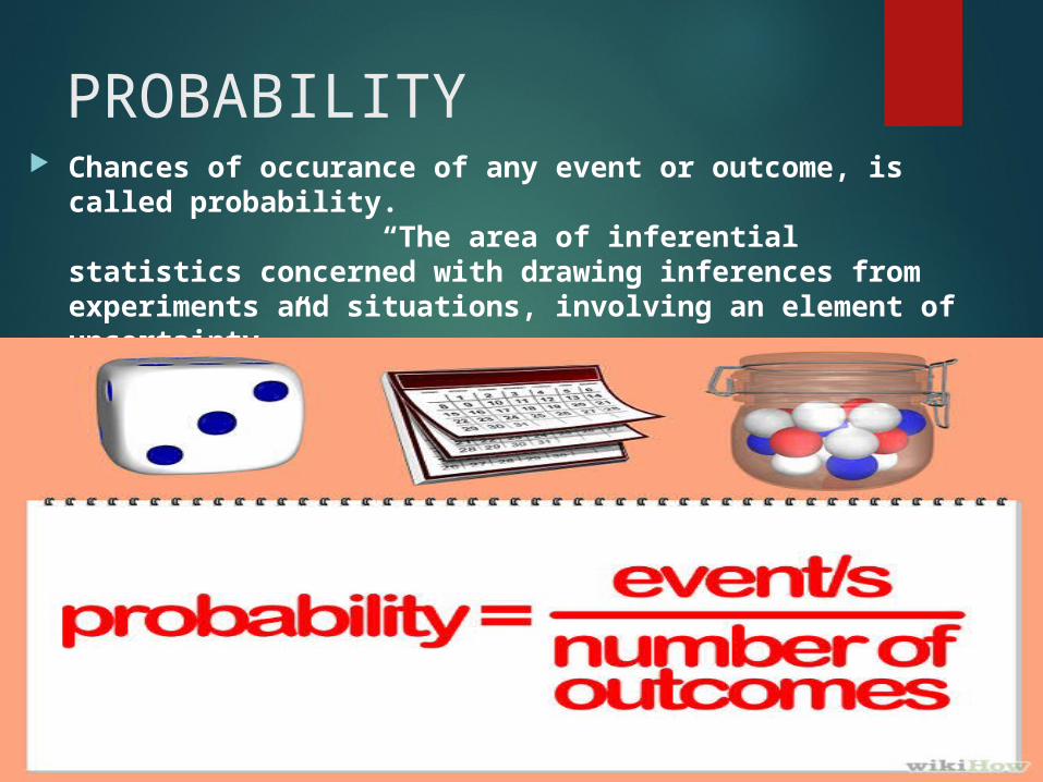
PROBABILITY Chances of occurance of any event or outcome, is

called probability. “The area of inferential statistics concerned with drawing inferences from experiments and situations, involving an element of uncertainty.”

Discrete Random Variable A discrete random variable is a random variable that has values that has either

a finite number of possible values or a countable number of possible values. Example: A single die is cast. The number of pips showing on the die.

The number of heads obtained in coin tossing experiments.

Interpretation Of The Mean of a Discrete Random VariableCompute the mean of the following probability distribution which represents the number of DVDs a person rents from a video store during a single visit.

FORMULA FOR MEAN μ = Σxp Mean=0*0.06+1*0.58+

2*0.22+3*0.1+4*0.03+5*0.01

Mean = 1.49

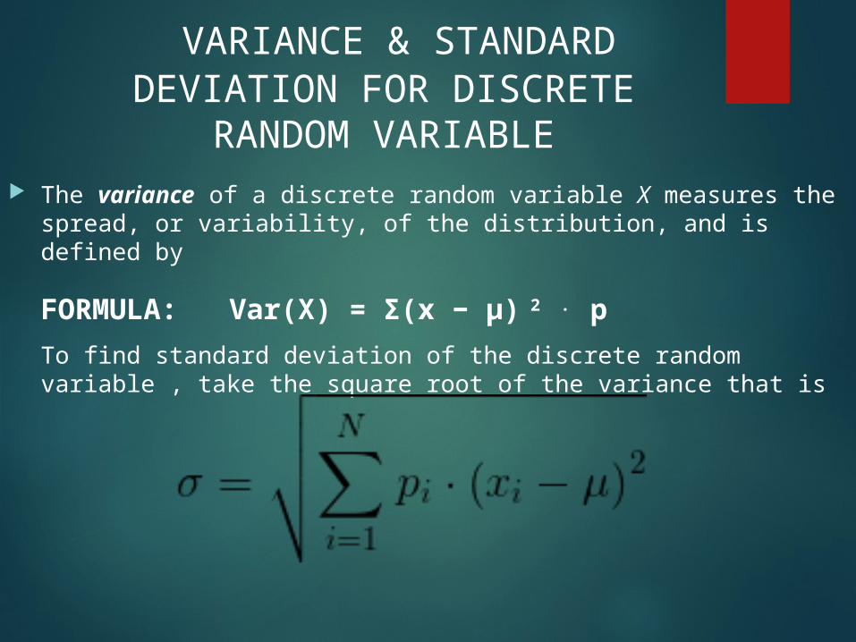
VARIANCE & STANDARD DEVIATION FOR DISCRETE

RANDOM VARIABLE The variance of a discrete random variable X measures the

spread, or variability, of the distribution, and is defined by

FORMULA: Var(X) = Σ(x − μ) 2 . p

To find standard deviation of the discrete random variable , take the square root of the variance that is

VARIANCE & STANDARD DEVIATION FOR DISCRETE RANDOM VARIABLE

The variance=(0-1.49)^2*0.06+(1-1.49)^2*0.58+(2-1.49)^2*0.22+(3-1.49)^2*0.1 +(4-1.49)^2*0.03+(5-1.49)^2*0.01

=0.8699

i.e Mean=1.49

Standard Deviation= 0.932684

BINOMIAL PROBABILITY DISTRIBUTION

Binomial Probability Distribution

A binomial experiment (also known as a Bernoulli trial) is a statistical experiment that has the following properties:

The experiment consists of n repeated trials. Each trial can result in just two possible outcomes. We

call one of these outcomes a success and the other, a failure.

The probability of success, denoted by P, is the same on every trial.

The trials are independent; that is, the outcome on one trial does not affect the outcome on other trials.

For Example success or failure

good & defective

Binomial Probability Distribution Example

Consider the following statistical experiment. You flip a coin 2 times and count the number of times the coin lands on heads. This is a binomial experiment because:

The experiment consists of repeated trials. We flip a coin 2 times.

Each trial can result in just two possible outcomes - heads or tails.

The probability of success is constant - 0.5 on every trial.

The trials are independent; that is, getting heads on one trial does not affect whether we get heads on other trials.

Application (Criteria) of Binomial Probability

Distribution

Fixed number of trials

Independent trials

Two different classifications

Probability of success stays the same for all trials

1. FIXED TRIALSThe experiment is performed a fixed number of times. Each repetition of the experiment is called a trial. E.g flip a coin 10 times thus fixed number of trials n=10. (fixed number of trials represented as n)

2. INDEPENDENT TRIALS

The trials are independent. This means the outcome of one trial will not affect the outcome of the other trials. E.g outcome of heads on the first flip will not affect the outcome of the second flip.

3. TWO CLASSIFICATIONSFor each trial, there are two mutually exclusive outcomes, success or failure.E.g A coin is flipped two times, each trial has two possible outcomes, heads(success) & tails(failure)

4. SAME PROBABILITIES

The probability of success is fixed for each trial of the experiment. The probabilities of successful trials must remain the same throughout the process we are studying. Flipping coins is one example of this. No matter how many coins are tossed, the probability of flipping a head is 1/2 each time.

E.g Probability of success (heads) is 0.50%Probability of failure (Tails) is 0.50= 50%Means equal chances of success and failure on flipping coin