Inferential statistics in the context of empirical...

JB[v.20020404] Prn:17/01/2007; 12:51 F: HCP1804.tex / p.1 (46-141)

Inferential statistics in the context of empiricalcognitive linguistics

Rafael Núñez

. Introduction

Imagine you read in a book about English grammar the following statement:

The regular plural marker in English is ‘s’, which is placed at the end of the noun as in

dog/dogs. There are, however, some exceptions like mouse/mice.

Then, you read in a book about child development a statement such as this one:

English speaking children have difficulties learning irregular forms of the plural.

The two statements make reference to a common subject matter, namely, English plurals,but they reflect deep differences in focus and method between the fields they belong to.The former statement is one about regularities and rules of a language (English), whilethe latter is a statement about patterns and regularities in the behavior or performance ofpeople who speak (or learn) that language. The latter is about phenomena that take placeat the level of individuals, while the former is about phenomena that lie beyond individualsthemselves. The former is the purview of linguistics, the latter, of psychology.

As an academic discipline one of the main goals of Linguistics is to study patterns andregularities of languages around the world, such as phonological structures and grammati-cal constructions like markers for tense, gender, or number, definite and indefinite articles,relative clauses, case marking of grammatical roles, and so on. Psychology, on the otherhand, studies people’s behavior, motivation, perception, performance, cognition, atten-tion, and so on. Over the last century, the academic fields of linguistics and psychologyhave developed following rather different paths. Linguistics, by seeing its subject matter asexisting at the level of structures of languages – beyond individuals themselves – gatheredknowledge mainly through the careful and detailed analysis of phonological and gram-matical patterns, by means of what philosophers of science and epistemologists call themethod of reasoning (Helmstadter 1970; Sabourin 1988). Psychology, on the other hand,by marking its definitive separation from Philosophy during the second half of the 19thCentury, defined its subject matter at the level of the individual and embraced a method ofknowledge-gathering which had been proved useful in the hard sciences: the experimentalmethod. Ever since, peoples’ behavior, performance, and mental activity began to be stud-

JB[v.20020404] Prn:17/01/2007; 12:51 F: HCP1804.tex / p.2 (141-195)

Rafael Núñez

ied with rigorously controlled experimental methods of observation and data gathering.An essential tool of the modern experimental method is Statistics, especially inferentialstatistics, which is a carefully conceived mathematically-based conceptual apparatus forthe systematic and rigorous analysis of the numerical data researchers get from their mea-surements.1 The main goal of this chapter is thus to characterize some key concepts instatistical reasoning in the context of empirical cognitive linguistics, and to analyze howinferential statistics fits as a tool for knowledge gathering in cognitive linguistics. The textis not meant to be a comprehensive introduction to statistics proper, for which the readermay consult any college textbook available, such as Witte & Witte 2007; Hinkle, Wiersma,& Jurs 2003; Heiman 2003, but is instead intended to introduce the topic in a way that ismeaningful for cognitive linguists.

. What counts as “empirical” in cognitive linguistics?

One important difference between linguistics and psychology has to do with the ques-tion of what counts as empirical evidence for falsifying or supporting a given theoreticalclaim. What is a well-defined valid piece of information that can be safely incorporatedinto the body of knowledge in the field? What counts as an acceptable method for ob-taining such a piece of information? When can that piece of evidence serve as a robustcounterargument for an existing argument? These are questions for which linguisticsand psychology traditionally have had different answers. For example, if some theory inlinguistics states that

the plural marker in language X is provided by a marker x,

then if through your detailed observations of the language you find a counterexamplewhere the plural marker is not x but y (i.e., well-accepted linguistic expressions that do notfit the proposed pattern) you can, with that very piece of information, falsify the proposedtheoretical statement. In such a case you would be making a contribution to the theoryafter which the body of knowledge would be modified to become something like

the regular plural marker in language X is provided by a marker x, but there are some

irregular cases such as y.

The same would happen if some linguistic theory describes some grammatical pattern tobe generated by a rule A, but then you observe that if you apply such a rule to some sen-tences you actually generate ungrammatical ones (which linguists usually write down pref-acing it with an asterisk). Again, by showing these ungrammatical sentences you wouldbe providing linguistic evidence against a proposed theoretical statement. You would befalsifying that part of the theory and you would be de facto engaging in a logical counter-argumentation, which ultimately would lead to the development of a richer and morerobust body of knowledge in that field.

. The history of Statistics as a field, however, reveals that its development not always came straightfor-

wardly from advances in mathematics (see Stigler (1986) for details).

JB[v.20020404] Prn:17/01/2007; 12:51 F: HCP1804.tex / p.3 (195-267)

Inferential statistics

The situation in psychology is quite different. Because the subject matter of psychol-ogy is not defined at the level of the abstract structure of a language as linguistics does,but defined at the level of peoples’ behavior (often used to infer people’s cognitive mecha-nisms), performance or production, the elements that will allow you to falsify or supporta theoretical statement will be composed of empirical data observed at the level of peo-ples’ behavior or performance. For instance in order to falsify or support a theoreticalstatement such as

English speaking children have difficulties learning irregular forms of the plural

you would have to generate a series of studies that would provide empirical data (i.e., viaobservation of real children), supporting or challenging the original statement. Moreover,you would have to make several methodological decisions about how to test the statement,as well as how exactly to carry out your experiments. For example, because you will notbe able to test the entire population of all English speaking children in the world (muchless those not yet born!), you will have to choose an appropriate sample of people whowould represent the entire population of English speaking children (i.e., you would beworking only with a subset from that population). And you will have to operationalizeterms such as “difficulties” and “learning” so it is unequivocally clear how you are going tomeasure them in the context of your experiment. And because it is highly unlikely that allindividuals in your sample are going to behave in exactly the same manner, you will needto decide how to deal with that variability, and how to characterize in some general butprecise sense what is going to be considered a “representative” behavior for your sample(i.e., how to establish a proper measure of central tendency), how to describe the degreeof similarity of children’s behavior, how to objectively estimate the error involved in anymeasurement and sampling procedure, and so on. Within the realm of the experimentalmethod all these decisions and procedures are done with systematic and rigorous rulesand techniques provided by statistical tools.

The moral here is that linguistics and psychology, for historical and methodologicalreasons, have developed different ways to deal with the question of how you gain knowl-edge and build theories, how you falsify (or support) hypotheses, how you decide whatcounts as evidence, and so on. Where the relatively new field of cognitive linguistics isconcerned, which gathers linguists and cognitive psychologists (usually trained within theframework of the experimental method), it is very important to:

(a) keep in mind the nature and the implications of these methodological differences, and(b) understand the complementarity of the two methods of knowledge-gathering as prac-

ticed in linguistics and experimental psychology.

Cognitive linguistics, emerging out of linguistics proper, and initially in reaction to main-stream Chomskian-oriented approaches, has made important contributions to the studyof human language and its cognitive underpinnings. This new field, however, relyingmainly on linguistic methods of evidence gathering has made claims not only about lan-guages, but also about the psychological reality of peoples’ cognition. For example, animportant subfield of cognitive linguistics, conceptual metaphor theory, has, for the lasttwenty-five years or so, described and analyzed in detail thousands of metaphorical expres-

JB[v.20020404] Prn:17/01/2007; 12:51 F: HCP1804.tex / p.4 (267-321)

Rafael Núñez

sions such as the teacher was quite cold with us today and send her my warm helloes (Lakoff& Johnson 1980; Lakoff 1993). The inferential structure of these collections of linguis-tic expressions has been modeled by theoretical constructs called conceptual metaphors,which map the elements of a source domain (corresponding in the above examples to thethermic bodily experience of Warmth) into a more abstract one in the target domain (inthis case, Affection). The inferential structure of the metaphorical expressions mentionedabove (and many more) is thus modeled by a single conceptual metaphor: Affection IsWarmth.2

But beyond the linguistic description, classification, and analysis of linguistic expres-sions using methods in linguistics proper, conceptual metaphor theory has made impor-tant claims about human cognition, abstraction, and mental phenomena. For instance, ithas claimed that conceptual metaphors are ordinary inference-preserving cognitive mecha-nisms. These claims, however, are no longer at the level of linguistic data or the structure oflanguages, but at the level of individuals’ cognition, behavior, and performance. Because ofthis, many psychologists believe that giving a list of (linguistic) metaphorical expressionsas examples does not provide evidence (in cognitive and psychological terms) that peopleactually think metaphorically. In other words, what may count as linguistic evidence ofmetaphoricity in a collection of sentences for linguists may not count as evidence for psy-chologists that metaphor is an actual cognitive mechanism in peoples’ minds. It is at thispoint where some psychologists react and question the lack of empirical “evidence” to sup-port the psychological reality of conceptual metaphor (Murphy 1997; Gibbs 1996; and seeGibbs in this volume). Moreover, how do we know that some of the metaphors we observein linguistic expressions are not mere “dead metaphors,” expressions that were metaphor-ical in the past but which have become “lexicalized” in current language such that theyno longer have any metaphorical meaning for today’s users? How do we know that thesemetaphors are indeed the actual result of real-time cognitive activity? And how can wefind the answers to such questions? These are reasonable and genuine questions, whichfrom the point of view of experimental psychology, need to be addressed empirically.

Cognitive linguistics, which is part of cognitive science – the multidisciplinary scien-tific study of the mind – is located at the crossroads of linguistics and cognitive psychologyand as such, has inherited a bit of both traditions. It is therefore crucial for this field thatthe search for evidence and knowledge be done in a complementary and fruitful way.

We are now in a position to turn to more technical concepts.

. Descriptive vs. inferential statistics

Statistics has two main areas: Descriptive and inferential. Descriptive statistics, which his-torically came first, deals with organizing and summarizing information about a collectionof actual empirical observations. This is usually done via the use of tables and graphs (like

. In conceptual metaphor theory usually the name of the mapping has the form X Is Y, where X is the

name of the target domain and Y the name of the source domain.

JB[v.20020404] Prn:17/01/2007; 12:51 F: HCP1804.tex / p.5 (321-377)


the ones you see in the business or weather report pages of your newspaper), and averages(such as the usual Grade Point Average, or GPA, you had in school). These tools serveto describe actual observed data, which often can be quite large (e.g., every single gradeyou got in every single class you took in school), in a simple and summarized form (SeeGonzalez-Marquez, Becker & Cutting this volume, for further details.)

Inferential statistics, on the other hand, was developed during the 20th century withthe goal of providing tools for generalizing conclusions beyond actual observations. Theidea is to draw inferences about an entire population from the observed sample. Theseare the tools that allow you to make conclusions, about, say “English speaking childrenlearning irregular plurals,” based on only a few observations of actual children (i.e., thefixed number of individuals constituting your sample, which is necessarily more limitedthan the entire population of English speaking children around the world). As we will see,making these kinds of generalizations – from a small sample to a huge general population –implies risks, errors, and making decisions about chance events. The goal of inferentialstatistics then is not to provide absolute certainty, but to provide robust tools to evaluatethe likelihood (or unlikelihood) of the generalizations you would like to make. Later wewill see how this is this achieved.

. Variables and experiments

Statistical analyses have been conceived to be performed on collections of numerical data,where numbers are supposed to represent, in some meaningful way, the properties or at-tributes under investigation. Needless to say, if your observations are based only on verbalnotes, sketches, interviews, and so on, you will not be able to perform statistical analysesdirectly on such raw material. In order to use statistics you will have to transform your rawdata, via a meaningful procedure, into numbers. Sometimes, of course, that is not possi-ble, or it is too pushy to do so, or it just does not make any sense to do it! In those cases,statistical analyses may simply not be the appropriate tools for your analyses (and youshould be aware of that). However, when the properties or attributes under investigation(e.g., “degree of difficulty of a task,” “College GPA average,” or “the time it takes to answera question”) can take on different values for different observations, they are technicallycalled variables.

Variables are extremely important in the context of experimental design, because theyare at the core of the process of investigating cause-effect relationships. As it is well-known,one of the main goals of scientific research is to describe, to explain, and to predict phe-nomena (i.e., effects) in terms of their causes. The main way this is usually done is bycarefully designing experiments where the investigator studies some specific variables,called independent variables, in order to determine their effect on the so-called depen-dent variables. The dependent variables are the ones that are measured by the investigator,which are expected to be affected by the independent variables. Independent variables aresometimes manipulated variables (when the experimenter directly manipulates the levelsof the variable to be studied, like deciding the dose of a particular drug she will be giving toher participants) and sometimes they are classifying variables (when the experimenter cat-

JB[v.20020404] Prn:17/01/2007; 12:51 F: HCP1804.tex / p.6 (377-447)

Rafael Núñez

egorizes the individuals according to some relevant criterion, for example, sex or medicalcondition).

Variables are also important in the context of correlational studies. In this case the in-vestigators’ goal is not to systematically manipulate an independent variable in order toobserve its effect on a dependent variable (thus establishing a cause-effect relation) butrather to examine two or more variables in order to study the strength of their relation-ship. Correlational studies provide useful tools for investigating patterns and degrees ofrelationships among many variables, but they do not say much about causation. Rather,they say what is related with what, and to what degree the relationship is strong (or weak).When the relationship between two variables is strong it is possible to make predictionsof values in one variable in terms of the other with an appropriate level of accuracy. Acorrelational study can determine, for example, that in general height and weight are twovariables that are correlated: Very short people tend to weigh less than very tall people,and vice versa. The relation, of course, is not perfect. There are people who are short butwith strong muscles and thick bones, and are therefore heavy, and also tall thin peoplewho are light. But overall, if you observe hundreds or thousands of people, you will con-clude that height and weight are quite related. There are specific statistical tools than canbe used to establish precisely (in numerical terms) the strength and degree of relationshipbetween variables. What is important to keep in mind is that the fact of establishing astrong relationship between two variables does not mean that we can directly make asser-tions about which one causes which one. We may establish that height and weight are verymuch related, but not because of this can we say, for instance, that “variations in heightcause variations in weight” or that “variations in weight cause variations in height.” Wecan say that height and weight are related (or very related, or even very strongly related)but we can not affirm which causes the other. Correlational studies are useful, however,to identify in a study with many variables with unknown behavior, which variables relatewith which ones. Once the related variables are identified, the investigator may proceedto further study if a cause-effect relationship is suspected. But, in order to answer to thatquestion, she will need to work within the framework of the experimental approach. Forthe rest of the chapter we will focus on the experimental dimension of empirical studies.

In order to better understand the concept of experimental design, consider a re-searcher who suspects that a drug G affects peoples’ performance in remembering two-syllable nonsensical words. This suspicion, which usually is theory-driven and is tech-nically called a research hypothesis, states that variations in the performance (dependentvariable) are expected to be produced, or explained by variations in the dosage of drug G(independent variable). In this example the dependent variable could be defined opera-tionally as “number of words correctly remembered from a list shown 15 minutes prior tothe evaluation.” In order to investigate her hypothesis empirically, our researcher will de-sign an experiment, which should allow her to evaluate whether or not different doses ofdrug G produce changes in the performance of remembering those words. Then, she willcollect a sample of people (hopefully selected randomly), and divide it into, say, four cate-gories A, B, C, D. She will give to participants in each of the 4 groups, a specific dose of thedrug: for instance, 10mg to those in group B, 40mg to those in group C, 100mg to thosein group D, and 0mg to those in group A (the four dosage groups are technically called

JB[v.20020404] Prn:17/01/2007; 12:51 F: HCP1804.tex / p.7 (447-506)


the levels of the independent variable, and they are usually determined by relevant informa-tion about the domain of investigation found in the literature). Then, through a carefullyand systematically controlled procedure, she will show them a long list of two-syllablenonsensical words, and 15 minutes later, she will measure the individuals’ performance(number of words remembered correctly) under the different dosage conditions (levels ofthe independent variable). She will then be ready to evaluate, using the tools of inferentialstatistics, whether the data support her hypothesis. (In reality, things are, of course, morecomplicated than this and get technical rather quickly, but for the purpose of this briefchapter we will leave it as it is.)

In this example, Group A plays a very interesting and important role. Why give 0mgto people in that group? Why bother? Why not simply eliminate that group if we are notgiving them any drugs at all? Well, here is where we can see one of the main ideas be-hind an experimental design: experimental control. What the experimenter wants is tosystematically study the possible cause-effect relationship between the independent anddependent variables. In our example, she wants to investigate how variations in drug Gdosage (independent variable) affect remembering nonsensical words (dependent vari-able). But she wants to do this by isolating the effect of the independent variable whilekeeping everything else (or as much as possible) constant, thus neutralizing possible ef-fects from extraneous variables. For instance, it could be the case that simply the testingsituation, such as the list of words used for the study, or the environmental conditionsin the room used for the testing, or the background noise of the computer’s fan, or thepsychological effect of knowing that one is under the “effect of a drug,” seriously affectpeoples’ performance in an unexpected way, and this, independently of the actual activechemical ingredient of the drugs. Well, we would only be able to control the potential in-fluence of such extraneous variables if we observe individuals in a group going through thefull experimental procedure with one crucial exception: they do not actually get any activechemical ingredient believed to affect performance (i.e., absence of the attribute definedby the independent variable: 0mg of the drug). This means that the individuals in thisgroup, known as the control group, should also get a pill, like everybody else in the study,except that, unbeknownst to them, the pill will not have the known active ingredient.

When studies like the one above are done properly, we refer to them as experiments,that is, controlled situations in which one (or more) independent variables (manipulatedor classifying ones) are systematically studied to observe the effects on the dependent vari-able. The experiments can, of course, get more complicated. Our researcher, for instance,could be interested in studying the effects of more than one independent variable on thedependent variable. Other than the dosage of drug G, she could be interested in investi-gating also the influence of the time elapsed after showing the list of nonsensical words.This could be done through the manipulation of the variable “time elapsed,” by measur-ing performance not only after 15 minutes of showing the list, but also at, say, 5 minutes,and 30 minutes, which would give a better sense of how time may affect performance. Orperhaps she could be interested in studying the influence of the number of vowels presentin the nonsensical words (thus manipulating the number of such vowels), or even in howgender may affect the dependent variable (in this case it would not be a manipulated in-dependent variable, but a classifying one), and so on. The more independent variables

JB[v.20020404] Prn:17/01/2007; 12:51 F: HCP1804.tex / p.8 (506-571)

Rafael Núñez

you include, the more detailed your analysis of how the dependent variable is affected,but also the more complicated the statistical tools get. So as a good researcher, you wantto maximize the outcome of describing, explaining, and making predictions about yourdependent variable, and to minimize unnecessary complications by systematically and rig-orously studying relevant variables. The choice of what variables, how many of them, andwhat levels of each of them you need to incorporate in your experiment is often not a sim-ple one. A beautiful experiment usually is one that explains a lot with only a few optimallychosen manipulations, the true mark of an experienced experimenter.

. Measuring and measurement scales

The process of assigning numbers to attributes or characteristics according to a set of rulesis called measurement. Measurement thus results in data collected on variables. In the ev-eryday sense of “measuring,” you measure, say, the temperature of a room by bringingin a thermometer and then reading the displayed value. But in the context of statisticalanalysis you are also measuring when, via a set of rules, you assign, say, the number “1” to“girls” and “0” to “boys” with respect to the variable “sex”, or “1” to “low performance,”“2” to middle performance,” and “3” to high performance” with respect to performance inremembering nonsensical words from a list. Depending on the properties of your measur-ing procedure, different measurements scales are defined. It is very important that we knowwhat measurement scale we are dealing with as they define the kind of statistical analysiswe will be allowed to perform on our data. Simpler measurement scales only allow theuse of simple statistical techniques, and more sophisticated measurement scales allow formore complex and richer techniques. The following are the four main measurement scalesone needs to keep in mind.

. Nominal scale

This is the simplest measurement scale, which classifies observations into mutually ex-clusive categories. This classification system assigns an integer to categories defined bydifferences in kind, not differences in degree or amount. For example, we use nominalmeasurements every time we classify people as either left- or right-handed and by assign-ing them the number 1 or 2, respectively. Or when we assign a number to individualsdepending on their countries of citizenship: 1 for “USA”, 2 for “Canada”, 3 for “Mexico”,and 4 for “other”. In these cases, numbers act as mere labels for distinguishing the cat-egories, lacking the most fundamental arithmetic properties such as order (e.g., greaterthan relationships) and operability (e.g., addition, multiplication, etc.). With nominalmeasurements, not only it is arbitrary to assign 1 to USA, and 3 to Mexico (it could bethe other way around), but also it does not make any sense to say that the “3” of Mexicois greater than the “1” of the USA, or that the “2” of Canada is one unit away from thecategory USA. Because of the lack of arithmetic properties, the data obtained by nominalmeasurements are referred to as qualitative data. As we will see later, the statistical analysisof this kind of data requires special tools.

JB[v.20020404] Prn:17/01/2007; 12:51 F: HCP1804.tex / p.9 (571-634)


. Ordinal measurement

This measurement scale is like the previous one in the sense that it provides a mutually ex-clusive classification system. It adds, however, a very important feature: order. Categoriesin this case, not only are defined by differences in kind, but also by differences in degree(i.e., in terms of greater-than or lesser-than relationships). For example, we use an ordinalmeasurement when we classify people’s socioeconomic status as “low”, “middle”, or “high”,assigning them the numbers 1, 2, and 3, respectively. Unlike in the nominal case, in ordi-nal measurements it does make sense to say that the value “3” is greater than “1”, becausethe category assigning the value “3” denotes higher socio-economic status than the cate-gory assigning the value “1”. This measurement scale is widely used in surveys, as well asin psychological and sociological studies, where, for instance, researchers classify people’sreplies to various questions as follows: 1=“strongly disagree”; 2=“disagree”; 3=“neutral”;4=“agree”; 5=“strongly “agree”.

Numbers, in ordinal measurements, have the fundamental property of order, and assuch they can be conceived as values placed along a dimension holding greater-than rela-tionships. These numbers however, lack arithmetic operability. Because of this reason, thedata obtained with ordinal measurements are also called qualitative data. Usually the sta-tistical analyses for analyzing these data require the same tools as those used for nominalmeasurements.

. Interval measurements

Interval measurements add a very important property to the ones mentioned above. Theynot only reflect differences in degree (like ordinal scales), but also have the fundamen-tal property of preserving differences at equal intervals. The classic example of intervalmeasurement is temperature as measured in Fahrenheit or Celcius degrees. Again, valuescan be conceived of as ordered along a one-dimensional line, but now they hold the extraproperty of preservation of equal intervals between units. Anywhere along the Fahrenheitscale, equal differences in value readings always mean equal increases in the amount of theattribute, which in the case of temperature corresponds to the amount of heat or molecu-lar motion. In these measurements, arithmetic differences between numbers characterizethe differences in magnitude of the measured attribute. This property guarantees that thedifference in amount of heat between, say, 46◦F and 47◦F, is the same as the one between87◦F and 88◦F (i.e., 1◦F). Numbers used in this scale then have some operational proper-ties such as addition and subtraction. Because of these arithmetic properties, the data arereferred to as quantitative data. One important feature of these measurements is that thevalue zero (e.g., 0◦F) is chosen arbitrarily: The value “zero” does not mean absence of theattribute being measured. In the case of the Fahrenheit scale, 0◦F does not mean that thereis absence of molecular motion, i.e. heat.

JB[v.20020404] Prn:17/01/2007; 12:51 F: HCP1804.tex / p.10 (634-737)

Rafael Núñez

. Ratio measurement

This is the most sophisticated measurement scale. It gives the possibility of comparing twoobservations, not only in terms of their difference as in the interval measurement (i.e.,one exceeding the other by a certain amount), but also in terms of ratios (e.g., how manytimes more is one observation greater than the other). Ratios and times require numbersto be operational under multiplication and division as well, and this is exactly what thismeasurement scale provides. And in order for the idea of “times” to make any sense at all,the ratio measurement defines a non-arbitrary true zero, which reflects the true absence ofthe measured attribute. For example, measuring peoples’ height or weight makes use ofratio measurements, where, because of a true zero (lack of height or weight, respectively)the measurement reads the total amount of the attribute. In these cases then, it does makesense to say that a father’s height is twice that of his daughter’s, or that the weight of a 150-pound person is half that of a 300-pound person. In the context of cognitive linguistics,examples of ratio measurements are “reaction time” or “numbers of words rememberedcorrectly,” where it is possible to affirm, for instance, that participant No 10 respondedthree times as fast as participant No 12 did, or that participant No 20 remembered only25% of the words remembered by participant No 35.

These kinds of comparisons provide rich information that can be exploited statisti-cally, but if there is no true-zero scale they cannot be made meaningfully. For instance, inthe case of temperature mentioned earlier, it is not appropriate to say that 90◦F is threetimes as hot as 30◦F. One could say, of course, that the difference between the two is 60◦F,but since the Fahrenheit scale lacks a true zero, no reference to ratios or times should bemade. Because of the arithmetic properties of ratio measurements (i.e., order, addition,subtraction, multiplication, division), ratio data are quantitative data allowing for a widerange of statistical tools.

As we said earlier, when we are measuring, it is very important to know with whatkind of measurement scale we are dealing with, because the type of scale will determinewhat kind of inferential statistical tests we will be allowed to use. Table 1 summarize theproperties discussed above.

. Samples and populations

A population is the collection that includes all members of a certain specified group. Forexample, all residents of California constitute a population. So do all patients following aspecific pharmacological therapy at a given time. As we saw earlier, when researchers insocial sciences are carrying out their investigations, they rarely have access to populations.Studying entire populations is often extremely expensive and impractical, and sometimessimply impossible. To make things tractable, researchers work with subsets of these pop-ulations: samples. Carrying investigations with a sample can provide, in an efficient way,important information about the population as a whole.

When samples are measured researchers obtain data, which is summarized withnumbers that describe some characteristic of the sample called statistics (this notion of

JB[v.20020404] Prn:17/01/2007; 12:51 F: HCP1804.tex / p.11 (737-781)


Table 1. Measurement scales

Scale Properties Observations reflectdifferences in

Examples Type of data

Nominal Classification Kind Sex; major in college; native

language; ethnic background

Qualitative

Ordinal Classification

Order

Degree Developmental stages; academic

letter grade;

Qualitative

Interval Classification

Order

Equal intervals

amount Fahrenheit temperature; Grade

Point Average*; IQ score*

Quantitative

Ratio Classification

Order

Equal intervals

True zero

total amount and

ratio

Reaction time; number of words

remembered; height; income

Quantitative

* Technically, these are ordinal measurements, but they have been built in such a way that they can be

considered interval measurements.

“statistics”, by the way, should not be confused with the one used in the terms “inferentialstatistics” or “descriptive statistics”). An example of a statistic is the sample mean, whichis a type of average, a measure of central tendency of the sample. Another example is thestandard deviation, which is a measure of variability of the sample (see Gonzalez-Marquez,Becker & Cutting this volume, for details on how to calculate these statistics). A statistic isthus a descriptive measure of a sample (e.g., the mean height of a sample of undergradu-ate students you take from your college). On the other hand, a measure of a characteristicof a population is called a parameter (e.g., the mean height of all undergaduate studentsin California). To distinguish between descriptive measures of samples and populations,two different kinds of symbols are used: Roman letters are used to denote statistics (sam-ple measures) and Greek letters are used to denote parameters (population measures).For example, the symbol for sample mean is X̄ (called “X bar”) and the symbol for thepopulation mean is µ (pronounced “mew”).

Statistics, which are numbers based on the only data researchers actually have, areused to make inferences about parameters of the population to which the sample belongs.But because every time a sample is taken from the general population there is a risk of notmatching exactly all the features of the population (i.e., the sample is by definition morelimited than the real population, and therefore it necessarily provides more limited infor-mation), there is always some degree of uncertainty and error involved in the inferencesabout the population. Luckily, there are many techniques for sampling selection that min-imize these potential errors, which, among others, determine the appropriate size of theneeded sample, and the way in which participants should be randomly picked.

The point is that we never have absolute certainty about the generalizations we makeregarding a whole population based on the observation of a limited sample. Those infer-ences will involve risks and chance events. We have to ask ourselves questions such as, Howlikely is it that the sample we are observing actually corresponds to the population that issupposed to characterize? Out of the many possible samples we can take from the popula-tion, some samples will look like the real population, others not so much, and others may

JB[v.20020404] Prn:17/01/2007; 12:51 F: HCP1804.tex / p.12 (781-829)

Rafael Núñez

actually be very different from the population. For example, imagine that we want to in-vestigate what the average height of undergraduate students is in all US college campuses.Since we do not have time or resources to measure every single student in the country,we take a sample of, say, 1000 students. Theoretically, we know that a good sample wouldbe one that appropriately characterizes the “real” population, where the sample’s statisticsmatch the population’s parameters (e.g., the sample mean corresponds to the populationmean µ, and the standard deviation of the sample is equal to the one in the populationwhich is designated by the Greek letter σ). But what are the chances that we get such asample? How about if due to some unknown circumstances we mostly get extremely tallpeople in our sample (e.g., if we happen to pick the student-athletes that are members ofthe basketball team)? Or perhaps, we get lots of very short people? In those unlikely casesour sample’s statistics will not match the populations parameters. In the former case, thesample mean would be considerably greater than the population mean, and in the latterit would be considerably smaller than the population mean. Here is where evaluating in aprecise way the likelihood of getting such rare samples becomes essential. This idea is atthe heart of hypothesis testing.

. Probabilities and the logic of hypothesis testing

In order to understand the logic of hypothesis testing, let us go back to our example in-volving the researcher who wanted to study the effects of drug G on people’s performancein remembering nonsensical words. Her general hypothesis was:

General Hypothesis:Drug G dosages affect people’s performance in remembering two-syllable nonsensicalwords.

Recall that in an experimental design, what the researcher wants is to investigate relevantvariables in order to establish cause-effect relationships between independent variables(often by directly manipulating them) and dependent variables. In order to keep the ex-planation of hypothesis testing simple, let us imagine that the researcher has decided tocompare the performance of a group of participants who took drug G with the perfor-mance of participants who did not (control group). In this case she will be testing thehypothesis that a specific dosage of drug G (independent variable), say 40 mg, affects theperformance in remembering two syllable nonsensical words, measured 15 minutes af-ter they had been shown (dependent variable). Her research hypothesis (which is morespecific than the general hypothesis) is then:

Research Hypothesis:A dosage of 40mg of drug G affects (increases or decreases) the performance of people inremembering two-syllable nonsensical words 15 minutes after presentation.

Let us now say that she randomly selects a sample of 20 participants (who will be supposedto characterize the vast population of “people” the hypothesis refers to. Keep in mind thatthe hypothesis does not say that the drug affects the performance of just these 20 par-

JB[v.20020404] Prn:17/01/2007; 12:51 F: HCP1804.tex / p.13 (829-890)


ticipants. Rather it says that it affects the performance of people in general). Then sherandomly assigns half of the participants to each group: 10 to group A (control group),and 10 to the experimental group (B) who will be given a dose of 40mg. After showingthem the list of two syllable nonsensical words in strictly controlled and well specified con-ditions (e.g., procedure done individually, in a special room in order to avoid distractions,etc.) she measures the number of words remembered by participants in each group andobtains the following results: on average participants in the control group remembered14.5 words, against an average of only 9 words in the experimental group.

At this point, the crucial question for the researcher is the following:

Can we simply say that the research hypothesis is supoprted? That drug G does ap-pear to affect (decrease, according to the results) people’s performance in rememberingnonsensical words?

Well, the answer is no. She can certainly say, from the point of view of descriptive statistics,that the mean number of words remembered by participants in the experimental group (9words) is smaller than the mean of those in the control group (14.5 words). But becauseher goal is to make inferences about the population of “people” in general based on herlimited sample, she has to evaluate the likelihood that the observed difference between thesample means is actually due to her experimental manipulation of drug G and not simplydue to chance. She will have to show that her results are a very rare outcome if obtained bychance, and therefore, that they can safely be attributed to the influence of drug G.

In inferential statistics, the way of reasoning is roughly the following: Any observedresult (like the difference in the average of recalled nonsensical words) is attributed tochance unless you have support to the contrary, that is, that the result is in fact a veryrare outcome that should not be attributed to mere chance. Inferential statistics providesmany powerful tools for evaluating these chances and determining the probability3 of theoccurrence of results. In our example, what our researcher needs to do is to run a statisticaltest to determine whether the difference she observed in the averages can be attributed tochance or not.

When running a statistical test, the researcher will have to specify even further herresearch hypothesis and state it in formal terms (called statistical hypotheses). Because thelogic underlying inferential statistics says that observed results are attributed to chanceuntil shown otherwise, the hypothesis is stated statistically in two steps. First, the nullhypothesis (H0) is stated, which formally expresses (usually) what the researcher wouldlike to disprove. Then the alternative hypothesis (H1) is stated, which formally expresses

. The probability of an event A, which is denoted as P(A), is expressed by a ratio: the number of out-

comes divided by the number of possible outcomes. The way in which this ratio is defined, determines

that a probability value is always greater or equal to zero (impossibility) and smaller or equal to one (ab-

solute certainty). For instance, the probability that after rolling a die you get the number 2 is 1/6, since

“2” is the only outcome, out of a total of six possible outcomes, that satisfies the condition expressed by

the event. Similarly, the probability that if you roll the dice twice you obtain an added result of 9 is 4/36,

which is equal to 1/9, because there are four outcomes out of thirty-six possible outcomes, that satisfy the

condition of adding up to 9. These four outcomes occur when the first die is 3 and the second is 6, when

they are 6 and 3, when they are 4 and 5, and 5 and 4, respectively.

JB[v.20020404] Prn:17/01/2007; 12:51 F: HCP1804.tex / p.14 (890-943)

Rafael Núñez

Figure 1. The normal distribution

the researcher’s belief, the contrary of what H0 states. Since at this level concepts have beencharacterized in terms of numbers and formal statements, H0 is the formal negation of H1.(i.e., usually it expresses the contrary of what the researcher wants to find evidence in favorof). In the drug G example, these statistical hypotheses would be expressed as follows:

Null hypothesis:H0: µA = µB

Alternative hypothesis:H1: µA �= µB

The alternative hypothesis states that the population mean to which the control groupbelongs (µA) differs from the population mean to which the experimental group receivingthe dose of drug G belongs (µB). The null hypothesis states the contrary: that H1 is nottrue, that is, µA is not equal to µB. Again, remember that statistical hypotheses are statedthis way because, as we said before, the logic of inferential statistics is to attribute anyobserved results to chance (H0), until you can show the contrary (H1).

In order to support the contrary possibility one has to show that the result is a veryrare outcome if attributed only to chance. Statisticians can calculate exactly how rare isthe result of an experiment performed on samples, by computing the probability of itsoccurrence with the help of theoretical distributions. An important distribution is the so-called normal curve, which is a theoretical curve noted for its symmetrical bell-shapedform, peaking (i.e., having its highest relative frequency) at a point midway along thehorizontal axis (see Figure 1).

The normal curve is a precious tool for modeling the distributions of many phe-nomena in nature. One such phenomenon, for instance, is the distribution of height ina population. Figure 2 displays the distribution of heights of a randomly selected sampleof 500 people. Height is shown as a variable on the horizontal axis, and proportion of oc-currence on the vertical axis. Intuitively, we can see that most people’s height falls aroundthe value in the middle of the horizontal axis (i.e., at that middle point on x the propor-tion y is the highest, namely at 68 inches), that fewer people are either very short or verytall (e.g., if you look either to the left or to the right of the middle point, the proportionsare smaller), and that even fewer are either extremely short or extremely tall (the propor-tions towards the extremes get smaller and smaller). If we get bigger and bigger samples,

JB[v.20020404] Prn:17/01/2007; 12:51 F: HCP1804.tex / p.15 (943-1012)


Figure 2. Distribution of heights of 500 people

our height data will progressively become more and more accurate in characterizing thedistribution of heights in the population, and the resulting graph will get closer and closerto the theoretical normal curve.

The actual normal distribution, which as such is never reached, is a theoretical toolthat has many important properties. One such property is that the theoretical middlepoint corresponds to the population mean, which other than being also the most frequentvalue, is the one that divides exactly the entire distribution into two halves (the normalcurve has, of course, many more important mathematical properties which we cannotanalyze here). For convenience, often we need to work with a standardized form of thenormal curve, which, for simplicity, has been set with a mean of 0 (µ = 0) and a standarddeviation (which indicates the degree of variability of the population, and it is denoted byσ) of 1 (σ = 1). As a consequence, in the standardized form values below the populationmean (0) are characterized in terms of negative numbers and those above the mean interms of positive numbers. Finally, another important property of the normal curve is thatit is always the case that 68% of all possible observations lie within 1 standard deviationfrom the mean, and approximately 95% of them lie within 2 standard deviation units(see Figure 1).

Keeping our drug G experiment in mind, the move now is to try to determine howrare is the difference of the observed sample means obtained by the researcher (a sam-ple mean of 14.5 words for the control group vs. 9 words for the experimental group).The logic then goes as follows. If drug G really does not produce any effect at all, thenwhatever difference we may obtain can be attributed to chance. In such a case, we wouldexpect the difference between the number of words remembered by the participants underthe innocuous drug G and the number of words remembered by the participants in thecontrol group, to be 0, or close to 0. So, if we think of the distribution we would obtain

JB[v.20020404] Prn:17/01/2007; 12:51 F: HCP1804.tex / p.16 (1012-1083)

Rafael Núñez

if we plotted the differences between the sample means (control minus experimental) ofall possible pairs of random samples of 10 individuals (which is the size our researcher isworking with) then we would obtain a theoretical normal distribution, technically calledthe sampling distribution of sample means differences. In this distribution, a difference of0 between the sample means would be considered a very common outcome because ithas the highest relative frequency. A positive but small difference between the two samplemeans would still be considered a relatively common outcome. So it would a small nega-tive difference (where the sample mean of the experimental group is higher than the oneof the control group). But a huge positive difference between the two sample means wouldindicate an extremely rare outcome if it was only attributed to chance (imagine the sam-ple mean of the control group being, say, 100 words, and the sample mean of the groupunder drug G being only 2 words). If we depicted such difference (the standardize valve of100 – 2 = 98) relative to its sampling distribution of sampling mean differences, the valuewould be located at the extreme right of the normal distribution whose relative frequency(y value) would be extremely small (i.e., highly unlikely to occur). Because the logic ofinferential statistics is to attribute any result to chance until shown otherwise, statisticianshave decided that in order to be extremely cautious, they would give the status of “rareoutcome” only to those that are really rare, and not just “relatively” rare or “quite” rareoutcomes. In numbers that means that they have decided to give the status of “rare out-come” only to those cases that are among the “rarest” 5%. The other 95% of cases are thussimply considered “common outcomes” (sometimes the criterion is even stricter, calling“rare outcome” only the 1% most rare, or even the 0.1% most rare, that is, those outcomesthat are so rare that if they are only attributed to chance they would occur in at most 1 ina thousand times).

When brought into the values of the horizontal axis of the normal distribution, thecriteria of “rare outcome” (e.g., the extremes 5%, 1%, or 0.1%) determine specific criticalvalues which will help decide whether the result the researcher is interested in evaluatingis a rare outcome or not. Based on this important idea of critical values, statistical testshave been conceived to produce specific numbers that reflect – numerically – how rare orcommon the results are (the underlying sampling distribution not always is the normaldistribution. There are many other kinds of distributions, but for the sake of simplicity wewill assume, for the moment, that the underlying distribution is normal). These numbersare compared to the critical values in order to decide which of the statistical hypothesis toreject and which one to accept: the null hypothesis H0 (which says that nothing extraor-dinary or unusual is happening with respect to some characteristic of the population) orthe alternative hypothesis H1, identified with the research hypothesis, which indicates thatsomething extremely unlikely is happening that should not be attributed to mere chance.When the underlying sampling distribution is the normal distribution, the extreme 5%(that is, the extreme 2.5% on each side of the curve) is determined by the critical value±1.96. If the statistical test produces a number that is greater than 1.96 or smaller than–1.96, we are in a position to reject the null hypothesis at a 5% level of significance (theoutcome would be considered rare). If the value falls between –1.96 and 1.96 we retain thenull hypothesis at 5% level of significance (the outcome would be considered common;see Figure 3).

JB[v.20020404] Prn:17/01/2007; 12:51 F: HCP1804.tex / p.17 (1083-1092)


Figure 3. The standard normal distribution and the areas of retention and rejection of the null

hypothesis

In our drug G example, if the value given by the appropriate statistical test (whichwe will see later) that evaluates the difference between the sample means of the groups(control minus experimental) is more extreme than the critical values (i.e., greater thanthe positive critical value on the right extreme of the normal curve, or smaller than thenegative critical value on the extreme left side of the curve), then we would reject thenull hypothesis and accept the alternative hypothesis. In such case we would concludethat the results observed in the experiment cannot be attributed to mere chance, and thatthey reflect the effect of the experimental manipulation (i.e., the effect of drug G). Theparticular test we would use in such case, which falls in the category of parametric infer-ential statistics, is called t-test (for two independent samples4). There are, of course, manydifferent inferential statistical tests that have been conceived for evaluating all sorts ofdata in different research designs (e.g., studies comparing three or more groups; studieswith independent samples and studies with repeated measures; studies with one, two, ormore independent variables; studies with one, two or more dependent variables; studiesin which certain assumptions, such as the one of the normal distribution, cannot be made;studies whose data is not quantitative but qualitative; and so on).

. Two independent samples refer to cases where observations in one sample are not paired with obser-

vations in the other one. A different version of the t-test for matched samples is used when the observations

across the two samples are paired. This would occur, for instance, in a study of married couples that has

the observation of each husband in one sample matched with the observation of the corresponding wife in

the other sample. It would also occur when each pair of observations belong to the same participant mea-

sured under different conditions or at different times, for example before and after a particular treatment

(this is also known as repeated measures design).

JB[v.20020404] Prn:17/01/2007; 12:51 F: HCP1804.tex / p.18 (1092-1148)

Rafael Núñez

In the remainder of the chapter we will analyze some examples of statistical tests.We will go over the main concepts involved in two parametric tests, namely, the t-test fortwo independent samples (with a numerical example) and the Analysis of Variance, betterknown as ANOVA. And we will analyze a non-parametric test, the χ2 (Chi-Square) test(with a numerical example). Let us now see the details of these statistical tests.

. Parametric vs. non-parametric inferential statistics

The kind of statistical tests researchers are able to use is determined by several factors suchas the type of measurement scale used to gather data (nominal, ordinal, interval, and ratioscales), and whether the technique has been conceived to test populations’ parameters ornot (there are other more technical criteria as well). When tests are about populations’parameters such as population means or population standard deviations, they are calledparametric tests. When tests do not evaluate population parameters but focus on otherfeatures such as frequencies per categories (i.e., number of cases) they are called non-parametric. Usually statistical tests based on quantitative data are parametric, because,as we said earlier, when the data is obtained with interval and ratio measurement scalesnumbers have full arithmetic properties, which allow statistics such as sample means to beused for making inferences about the parameters of populations (e.g., population means).In other situations, when statistical tests do not focus on parameters, but in frequencies,we use non-parametric tests.

. t-test, a parametric test

Let us go back to our example of whether drug G affects performance in rememberingnonsensical words. The research hypothesis in that experiment is that a dosage of 40mgof drug G affects (increases or decreases) the performance of people in remembering two-syllable nonsensical words 15 minutes after presentation. Stated that way, the hypothesisdoes not specify in what way drug G “affects” performance, whether it increases or de-creases performance. In such case, if the statistical test to be used makes use of the normaldistribution (or the t distribution), the test is said to be two-tailed or nondirectional (i.e.,the rejection areas are located at both tails of the distribution). But let us imagine thatour researcher has more specific knowledge about drug G and that she is in a position toconceive a more specific experimental hypothesis:

Experimental hypothesis:A dosage of 40mg of drug G affects (in fact decreases) the performance of people inremembering two-syllable nonsensical words 15 minutes after presentation.

Then she will require the use of a one-tail or directional test. By making the hypothesisthat drug G decreases performance she is saying that she expects the difference between themeans (control minus experimental) to be positive, therefore the rejection area is locatedin just one tail of the distribution (the positive side). The statistical hypotheses can nowbe specified as follows:

JB[v.20020404] Prn:17/01/2007; 12:51 F: HCP1804.tex / p.19 (1148-1251)


Null hypothesis:H0: µA – µB ≤ 0

Alternative hypothesis:H1: µA – µB > 0

The difference of the population means (control minus experimental) is thus expected tobe greater than zero (i.e., a dosage of 40mg of drug G decreases the performance of peoplein remembering two-syllable nonsensical words 15 minutes after presentation).

Let us now analyze the results obtained by our researcher. Here is the data:

Number of recalled words

Participant Control Experimental

No Group (A) Group (B)

1 16 9

2 13 8

3 12 7

4 14 9

5 13 11

6 14 12

7 17 11

8 16 8

9 18 7

10 12 8

No of participants in each group (n): 10 10

Total sum of scores (∑

X): 145 90

Sample Mean (∑

X/n)

Total sum/No of participants 145/10 = 14.5 90/10 = 9

In order to perform the t-test for two independent samples (which is the test recom-mended in this case, assuming that the underlying distributions are close enough to thenormal distribution) we need to compute the following value:

t =(XA – XB) – (µA – µB)hyp

sXA – XB

But what does this formula mean? The value t will ultimately tell us whether the differenceobserved between the groups is rare or not. The greater the value of t, the more unlikelythat the observed difference can be attributed to chance. If we look at the formula (ig-noring the denominator sXA – XB for the moment), we can see that the value of t increaseswhen the numerator increases, that is, when the difference between the sample means(XA – XB) and the populations means (µA – µB)hyp increases. And this difference increaseswhen the difference between the sample means (XA – XB) is greater than the difference be-tween (µA – µB)hyp. Since the value of (µA – µB)hyp represents the hypothesized differencebetween population means (taken to be zero), then the crucial element that determineshow big the value of t is going to be is the difference between the sample means (XA –XB). If the sample means XA and XB are similar, then their difference is very small, and

JB[v.20020404] Prn:17/01/2007; 12:51 F: HCP1804.tex / p.20 (1251-1336)

Rafael Núñez

t has a value close to zero. Such a small value of t, when compared to the critical valuesmentioned earlier (which ultimately determine what value of t the observed results aregoing to be called rare), will indicate that the little difference between the sample meanscan be attributed to chance, and therefore the null hypothesis H0 is accepted (and the al-ternative hypothesis H1 is rejected). But if XA, the sample mean of the control group A, ismuch greater than XB, the sample mean of the experimental group B, then that differencewill be translated into a larger t value. If the t value is greater than the critical value thatdetermines the limit of the rarest 5% (0.05 level of significance) then we can safely assumewith a 95% of certainty that the observed difference between the sample means is a rareoutcome if attributed to chance, and therefore we can reject the null hypothesis H0 andaccept the alternative hypothesis H1.

In order to compute the actual value of t, we need to perform several calculations. Letus go step by step:

1) We know that the number of participants in each group is 10 (nA = 10, and nB = 10),and that

2) the total sum of scores per group is∑

XA = 145 for the control group, and∑

XB = 90for the experimental group.

For reasons that we will not analyze here, we will also need some other calculations:

3) The sums of the squares of the scores per group:∑X2

A = 2143 and∑

X2B = 838 (you can compute these numbers, by squaring each

score and by adding them for each group).4) An estimated measure of the variability of the sampling distribution of sample means

differences (technically called estimated standard error of sXA – XB , but whose details wewill skip here. We will simply retain that, roughly speaking, this value expresses theaverage amount by which (XA – XB) will deviate from its expected value by chance).Their computation is given by:

5)

s2A =

nA(∑

X2A) – (

∑XA)2

nA(nA – 1)s2B =

nB(∑

X2B) – (

∑XB)2

nB(nB – 1)

By substituting the numbers from our example into the formulae we obtain:

s2A =

10(2143) – (145)2

10(10 – 1)s2B =

10(838) – (90)2

10(10 – 1)

s2A =

21430 – 21025

10(9)s2B =

8380 – 8100

10(9)

s2A =

405

90= 4.5 s2

B =280

90= 3.1

6) With the value obtained in (4), we can now estimate the population variance with thepool variance estimate s2

p, based on a combination of the two sample variances. Sincen is the same in both groups (n = 10) this number will turn out to be an average of s2

A

and s2B, namely 3.8.

JB[v.20020404] Prn:17/01/2007; 12:51 F: HCP1804.tex / p.21 (1336-1412)


7) We then compute the denominator of the t ratio, sXA – XB :

sXA – XB =√

[(s2p/nA) + (s2

p/nB)] =√

[(3.8/10) + (3.8/10)] =√

[(0.38) + (0.38)]

=√

(0.76) = 0.87

Finally, we can compute our t ratio by substituting our numbers into the formula givenabove:

t =(XA – XB) – (µA – µB)hyp

sXA – XB

=(14.5 – 9) – 0

0.87= 6.32

And we can compare our t ratio with the critical value that determines what differencebetween sample means are we going to consider a rare outcome. Critical values are usuallyfound in special tables built after the corresponding distributions that, depending on thesize of the samples (which determines what is called the number of degrees of freedom ofthe distribution) and the targeted level of significance (i.e., whether we want to call a rareoutcome only those among the rarest 5%, 1%, or 0.1%), give you the critical value againstwhich we have to compare our value in order to decide whether to reject or accept thenull hypothesis H0 (In this case, our t value is compared not with values from the normaldistribution, but from a similar distribution, the t distribution5). In our example, afterlooking at the tables (with the appropriate of degrees of freedom, 10 – 1 = 9 step which wewill skip here) we see that the critical values for a one-tailed test and for a group samplesize of n = 10, are 1.833 for a 5% level of significance, 2.821 for a 1%, and 4.297 for a 0.1%(notice that the values are increasingly bigger as we are more and more strict in decidingwhat are we going to call a “rare” event). Since the t ratio based on the drug G data is 6.32,which is greater than 4.297, the most strict critical value (0.1%), we decide to reject thenull hypothesis at a .01% level of significance and accept the alternative hypothesis.

We are finally in a position to answer the original question: Does drug G decreasepeople’s performance in remembering two-syllable nonsensical words? The experimentaldata obtained by our researcher allows us, via the t-test, to support the research hypothesisthat said that drug G diminishes people’s performance in remembering those words. Thepurely numerical result of the t-test can now be interpreted by saying that the differencebetween the number of two-syllable nonsensical words recalled by the participants in thetwo groups was big enough (control group being greater than the experimental group)that if it were to be attributed to chance it would be an extremely rare event occurring, atmost, once every thousand times. Therefore, the fact that the performance of participantsin the experimental group (B) who received drug G was lower than the one of participantsin the control group (A) can safely be attributed to the performance-decreasing effect ofdrug G. This result thus provides empirical (experimental) evidence supporting the claim

. The sampling distribution of t is almost equal to the standard normal distribution when the samples

are higher than 30 observations (being equal to it at the theoretical case when there is an infinite number

of observations). The t distribution has slightly inflated tails and its peak point is lower than the standard

normal distribution. These features are more apparent when the samples are small.

JB[v.20020404] Prn:17/01/2007; 12:51 F: HCP1804.tex / p.22 (1412-1477)

Rafael Núñez

that the decreased performance in the word recall task while taking drug G is very unlikelyto be the result of chance.

. Analysis of Variance (ANOVA), a parametric test

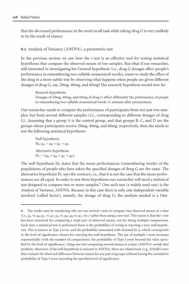
In the previous section we saw how the t-test is an effective tool for testing statisticalhypotheses that compare the observed means of two samples. But what if our researcher,still interested in investigating her General hypothesis (i.e., drug G dosages affect people’sperformance in remembering two-syllable nonsensical words), wants to study the effect ofthe drug in a more subtle way by observing what happens when people are given differentdosages of drug G, say, 20mg, 40mg, and 60mg? Her research hypothesis would now be:

Research hypothesis:Dosages of 20mg, 40mg, and 60mg of drug G affect differently the performance of peoplein remembering two-syllable nonsensical words 15 minutes after presentation.

Our researcher needs to compare the performance of participants from not just two sam-ples, but from several different samples (i.e., corresponding to different dosages of drugG). Assuming that a group A is the control group, and that groups B, C, and D are thegroups whose participants receive 20mg, 40mg, and 60mg, respectively, then she needs totest the following statistical hypotheses:

Null hypothesis:H0: µA = µB = µC = µD

Alternative hypothesis:H1: ∼(µA = µB = µC = µD)

The null hypothesis H0 states that the mean performances (remembering words) of thepopulations of people who have taken the specified dosages of drug G are the same. Thealternative hypothesis H1 says the contrary, i.e., that it is not the case that the mean perfor-mances are all equal. In order to test these hypotheses our researcher will need a statisticaltest designed to compare two or more samples.6 One such test (a widely used one) is theAnalysis of Variance, ANOVA. Because in this case there is only one independent variableinvolved (called factor), namely, the dosage of drug G, the analysis needed is a One-

. The reader may be wondering why not use several t-tests to compare two observed means at a time

(i.e., µA vs. µB; µA vs. µC; µA vs. µD; µB vs. µC; etc.) rather than using a new test. The reason is that the t-test

has been conceived for comparing a single pair of observed means, not for doing multiple comparisons.

Each time a statistical test is performed there is the probability of erring in rejecting a true null hypoth-

esis. This is known as Type I error, and the probability associated with denoted by α, which corresponds

to the level of significance chosen for rejecting the null hypothesis. The use of multiple t-tests increases

exponentially (with the number of comparisons) the probability of Type I error beyond the value speci-

fied by the level of significance. Using one test comparing several means at a time (ANOVA) avoids that

problem. Moreover, if the null hypothesis is rejected in ANOVA, there are related tests (e.g., Scheffé’s test)

that evaluate the observed difference between means for any pair of groups without having the cumulative

probability of Type I error exceeding the specified level of significance.

JB[v.20020404] Prn:17/01/2007; 12:51 F: HCP1804.tex / p.23 (1477-1564)


way ANOVA (there are also more complex variations of ANOVA for repeated measuresdesigns, for two factors, and so on).

The overall rationale of ANOVA is to consider the total amount of variability as com-ing from two sources – the variability between groups and the variability within groups –and to determine the relative size of them. The former corresponds to the variabil-ity among observations of participants who are in different groups (receiving differentdosages of the drug), and the latter corresponds to the variability among the observationsof participants who receive the same treatment. If there is any variation in the observa-tions of participants belonging to the same group (i.e., receiving the same dosage of thedrug), that variation can only be attributed to the effect of uncontrolled factors (randomerror). But if there is a difference between group means it can be attributed to the combi-nation of random error (which, being produced by uncontrolled factors, is always present)plus the effect due to differences in the experimental treatment (treatment effect). In otherwords, the more the variability between groups exceeds the variability within groups, thehigher the support for the alternative hypothesis (and the more the null hypothesis be-comes suspect). This idea can be expressed arithmetically as a ratio, known as the F ratio:

F =Variability between groups

Variability within groups

This ratio is, in certain respects, similar to the t ratio analyzed in the previous section.As we saw there, the t ratio – used to test the null hypothesis involving two populationmeans – corresponds to the observed difference between the two sample means dividedby the estimated standard error (or pooled variance estimate s2

p). The F ratio expressesa similar idea but this time it involves several sample means: the numerator characterizesthe observed differences of all sample means (analogous to t’s numerator, and measured asvariability between groups), and the denominator characterizes the estimated error term(analogous to t’s pooled variance estimate, and measured as a variability within groups).

The F ratio can then be used to test the null hypothesis (H0: µA = µB = µC = µD) thatall population means are equal, thus defining the F test7:

F =Random error + treatment effect

Random error

If the null hypothesis H0 really is true, it would mean that there is no treatment effectdue to the different dosages of drug G. If that is the case, the two estimates of variability(between and within groups) would simply reflect random error. In such case the contri-bution of the treatment effect (in the numerator) would be close to 0, and therefore the Fratio would be close to 1. But if the null hypothesis H0 really is false, then there would be atreatment effect due to the different dosages. Although there would still be random errorin both, the numerator and denominator of the ratio, this time the treatment effect (whichgenerates variability between groups) would increase the value of the numerator resultingin an increase of the value of F. The larger the differences between observed group means

. The F ratio has, like the t ratio, its own family of sampling distributions (defined by the degrees of

freedom involved) to test the null hypothesis.

JB[v.20020404] Prn:17/01/2007; 12:51 F: HCP1804.tex / p.24 (1564-1622)

Rafael Núñez

the larger the value of F, and the more likely that the null hypothesis will be rejected. Inpractice, of course – like in any statistical test – we never know whether the null hypoth-esis is true or false. So, we need to assume that the null hypothesis is true (which saysthat any observed differences are attributed to chance) and to examine the F value relativeto its hypothesized sampling distribution (specified, like in the case of the t-test, for thecorresponding degrees of freedom).8

So, how exactly is the value of the observed F calculated?9 Mathematically, ANOVAbuilds on the notion of Sum of Squares (SS), which is the sum of squared deviations of theobservations about their mean.10 In other words, the SS is the technical way of expressingthe idea of “positive (squared) amount of variability” which is required for characterizingthe meaning of the F ratio. In ANOVA there are various SS terms corresponding to thevarious types of variability: SSbetween (for between groups), SSwithin (for within groups),and SStotal for the total of these two. When the SSbetween and SSwithin are divided by theircorresponding degrees of freedom (the former determined by the number of groups, andthe latter by the number of observations minus the number of groups), we obtained a sortof “average” amount of squared variability produced by both, between group differencesand within group differences. These “averages” are variance estimates and are technicallycalled Mean Squares (MS): MSbetween (for between groups), MSwithin (for within groups).The F ratio described above is precisely the division of these two Mean Squares:

F =MSbetween

MSwithin

This value of F is then compared to the critical value associated to the hypothesizedsampling distribution of F for specific degrees of freedom, which are determined by thenumber of observations and the number of groups, and for the specified level of signif-icance. If based on her data, our researcher’s observed F value is greater than the criticalvalue, then the null hypothesis (that stated that all populations means were equal) isrejected, and she can conclude that different dosages of drug G differentially affect theperformance in recalling nonsensical words.

. The hypothesized sampling distribution of F is quite different from the normal distribution analyzed

earlier. Unlike the standardized normal distribution and the t distribution, which are symmetrical relative

to the axis defined by the mean (0) thus having negative values on one side and positive on the other,

the F distribution only has positive values. This is due to the fact that, mathematically, the variabilities

between groups and within groups are calculated using sums of squares (i.e., the sum of squared deviations

of the observations about their mean), which are always positive. Because of this reason, the F-test is a

nondirectional test.

. The actual calculations for a complete analysis of variance are far too lengthy for the space allotted.

Please see the statistical textbooks referenced here.

. The differences are squared in order to avoid a problem inherited from a simple property of the

mean: the sum of all the deviations of the observations about the mean equals zero. Squaring non-

zero deviations always produces positive numbers, and therefore it eliminates the problem of having the

deviations “canceling” each other out. A sum of squares is thus always greater or equal than zero.

JB[v.20020404] Prn:17/01/2007; 12:51 F: HCP1804.tex / p.25 (1622-1692)


. χ2 (Chi-Square), a non-parametric test

Now let us look at a statistical test that it is often used when the data is qualitative orobtained in categorical form. In order to illustrate this technique let us analyze a researchexample in the study of conceptual metaphor.

Cognitive linguists have analyzed many languages around the world noticing that inall of them, spatial language is recruited to talk about time. As in any conceptual metaphor,the theory says, the inferential structure of target domain concepts (time, in this case) isvia a precise mapping drawn from the source domain (uni-dimensional space, in thiscase). After examining hundreds of English expressions involving time, Lakoff and John-son (1980) identified two different metaphorical cases, Time Passing Is Motion of anObject (as in the expression Christmas is coming) and Time Passing Is Motion Overa Landscape (e.g., we are approaching the end of the month) (Lakoff 1993). The for-mer model (the Moving-Time version) has a fixed canonical observer where times areseen as entities moving with respect to the observer (Figure 4), while the latter (theMoving-Ego version) sees times as fixed objects where the observer moves with respectto time (Figure 5).

Psychologists have since questioned whether there is any psychological reality in peo-ple’s minds when they listen to, or utter, such metaphorical expressions (see, for exampleMurphy 1997). Is it the case that people actually operate cognitively with these concep-tual metaphors? Or could it be the case, as some scholars have argued, that the temporalmetaphorical expressions are simply “dead metaphors,” that is, expressions that once hadspatial content but that now have become separate temporal lexical items, no longer with

Figure 4. A graphic representation of the Time Passing Is Motion of an Object metaphor

Figure 5. A graphic representation of the Time Passing Is Motion Over a Landscape metaphor

JB[v.20020404] Prn:17/01/2007; 12:51 F: HCP1804.tex / p.26 (1692-1734)

Rafael Núñez

connections with space? Psychologists have tried to answer some of these questions us-ing priming techniques, a well-known experimental paradigm in which participants aresystematically biased via specific stimulation involving the source domain in order toevaluate whether they carry the corresponding inferences into the target domain. If bypriming the source domain of the metaphor (spatial) one gets systematic variation in theinferences made in the target domain, then one could conclude that individuals do rea-son metaphorically, or otherwise they would not be sensitive to the priming. With thisparadigm psychologists have gathered experimental evidence that indeed real or repre-sented physical motion scenarios can prime different construals of time (Boroditsky 2000;Gentner, Imai, & Boroditsky 2002). For example, speakers who have just been moving(e.g. traveling on a plane or a train) or imagining self-motion are primed to give Moving-Ego rather than Moving-Time interpretations of metaphorical time phrases in English,such as “the Wednesday meeting was moved forward two days.” This phrase can be inter-preted according to either of two mappings, Ego-moving or Time-moving; if Time is seenas moving towards Ego, then earlier events are “ahead of” later ones, and the meeting isseen as rescheduled to an earlier time (Monday); while if Ego is moving through space,then farther future events are farther ahead relative to Ego, so moving the meeting aheadis seen as rescheduled to a later time (Friday). With a priming background of self-motion,respondents’ interpretation is thus biased towards understanding forward as “to a latertime” (i.e., via Moving-Ego metaphor).

But can we really assume that people replying “Monday” rather than “Friday” aremaking the inferences in terms of a temporal motion “towards Ego”? Perhaps in the caseof “Monday” answers, what people are doing is to make inferences in terms of the refer-ence point (RP) in a sequence where the presence of an Ego is completely irrelevant. Insuch case, we would have a more primitive mapping where in front of the sequence is earlierand behind is later (Figure 6), without reference to any Ego (which in the target domainwould bring the moment “Now”). This more fundamental metaphor (called Time-RP asopposed to Ego-RP, by Núñez and Sweetser (2006), would model linguistic expressionssuch as spring follows winter or National Public Radio’s announcement twenty minutesahead of one o’clock (to refer to 12:40) which recruit dynamic language but where there isno reference to the present “now.”11 Núñez (1999) and Moore (2000) have already pro-vided linguistic and theoretical analysis of such more elementary metaphorical case. Butwhat can be said of the psychological reality of this Time-RP metaphor? What we wouldneed now is not to add more linguistic examples to the list of expressions, but to gatherempirical evidence of its psychological reality.

Later Earlier

Figure 6. A graphic representation of the Time-RP metaphorical construal of time

. An Ego, of course, could be added to this mapping (thus bringing a “Now”), resulting in the so-called

Time Passing Is Motion of an Object (Figure 4). But such a case wouldn’t be a primitive mapping but a

more complex composite one.

JB[v.20020404] Prn:17/01/2007; 12:51 F: HCP1804.tex / p.27 (1734-1808)


Figure 7. Example of the priming stimulus which was presented dynamically going from one side

of the screen to the other

So, coming back to the ambiguous expression “the meeting was moved forward,” ifparticipants reason in terms of this metaphorical mapping, then “to move forward” wouldbe seen as moving towards earlier moments in the sequence without having to refer to anEgo (i.e., now). This could be stated as a research hypothesis:

Research hypothesis:The proportion of people responding “Monday” to the ambiguous sentence “Wednesday’smeeting has been moved forward two days. When is the meeting?” will increase, if they areprimed with a visual stimulus showing a simple sequence of cubes going from one side tothe other of the computer screen.

In order to test such a hypothesis, in my lab we conducted an experiment in which themain goal was to prime the (spatial) source domain with an Ego-less sequence of cubesmoving on the screen from one side to other (see Figure 7). The idea was to see whetherparticipants would get prompted to give “Monday” replies just by looking to a simplesequence of moving cubes (with no reference whatsoever to an Ego). To avoid the biasthat a left-to-right vs. right-to-left presentation would produce, the priming stimulationwas done in a counterbalanced way. Participants in the control group observe only a staticverb of the cubes.

134 students participated in the study, half of which were in the control group (nopriming) and half in the experimental group (with priming). The statistical hypothesesare the following:

Null hypothesis:H0: Pc = Pe

Here Pc denotes the proportion of people in a non-primed population replying “Mon-day” rather than “Friday” to the above question (control), and Pe denotes the proportionof people answering “Monday” in a population primed with the visual stimulus (experi-mental). The null hypothesis says that the proportions are the same.

Alternative hypothesis:H1: Pc �= Pe

As usual, the alternative hypothesis states that the null hypothesis is false, that is, that theproportions of the two populations are different.

The following are the results of the experiment. The table below shows the number ofparticipants categorized according to their answers. The numbers indicate the frequencyof occurrence for each cell. Because the data here have been measured with a nominal scalethe data are considered qualitative (participants’ have been categorized according to theirresponses, “Monday” or “Friday”). With this kind of data the statistical test we can use in

JB[v.20020404] Prn:17/01/2007; 12:51 F: HCP1804.tex / p.28 (1808-1891)

Rafael Núñez

order to answer which statistical hypothesis is correct is the one-way χ2 (Chi-Square) test.This test is a non-parametric test because it does not deal with specific parameters of thepopulation such as population means, but rather it deals with frequency of occurrence ofcategorical observations.

Monday Friday TotalPriming (Exp.) 42 25 67No priming (Control) 26 41 67

Total 68 66 134

At a first glance we can see that without any priming more participants replied “Friday”to our question. In our sample, about a 61% of the participants in the control group(non-primed) replied “Friday” (41 participants out of 67), and a 39% of them replied“Monday” (26 out 76 participants). This set of data goes in the same direction as thefindings reported by Boroditsky (2000), where 54% of the participants responded “Friday”and 46% responded “Monday.” If we look at the participants in the experimental group(primed), however, the proportion of “Monday” replies (42 out of 67, or 63%) is greaterthan the proportion of “Friday” replies (25 out of 67, or 37%). We now need to use the χ2

test in order to determine whether this difference in proportions is a rare outcome if weattribute it to chance or not.

Like with the t-test, we need to calculate a value (χ2) which we will compare withits hypothesized sampling distribution (which this time is different from the normaldistribution. For details see any specialized text). The calculation is done with thefollowing formula:

χ2 =∑ (fo – fe)2

fe

where fo denotes the observed frequency of “Monday” and “Friday” responses from par-ticipants in the experimental group, and fe denotes the expected frequency for each cat-egory (“Monday” and “Friday”) from participants in the experimental group. “Expectedfrequency”, in this example, means that if participants do not go through any special treat-ment (such as the priming stimulation the participants in the control group were exposedto), then that is the frequency of “Monday” and “Friday” responses one would expectto encounter in the unprimed population. We can see that, as with the t-test, the valueof χ2 will increase if the numerator increases. And the numerator increases if the sumof the squared differences between the frequencies of the control group and the experi-mental group increases (The differences are squared, thus guaranteeing that the value willbe always positive and therefore the amount of differences will cumulate only in positiveterms). In short, we will get a big χ2 if the differences between expected and observed fre-quencies are big, and it will be small, or close to zero, if those differences are small. Thetest will help us determine if the differences we found between expected and observedfrequencies are significantly large or not. The following is the computation of χ2 for theresults of the above experiment:

χ2 =∑ (fo – fe)2

fe=

(42 – 26)2

26+

(25 – 41)2

41=

256

26+

256

41= 16.09

JB[v.20020404] Prn:17/01/2007; 12:51 F: HCP1804.tex / p.29 (1891-1952)


When compared to the appropriate sampling distribution of χ2 (with corresponding de-grees of freedom), the obtained value χ2 = 16.09 is greater than the critical values at 5%,1%, and even 0.1%, which are 3.84, 6.63, and 10.83, respectively.

So we can now reject, with a .01% level of significance, the null hypothesis H0

(which says that the proportions of people replying “Monday” rather than “Friday” inboth groups are similar), and accept the alternative hypothesis H1: The proportions of“Monday” responses are indeed (very) different (being that proportion greater in the ex-perimental group). And the difference is so big that if we were to attribute it to chance, itwill occur at most one in a thousand times.

In terms of the research question, the interpretation of this result is that a visualstimulus composed of an Ego-less sequence of cubes, which intervenes at the level of thespatial source domain of the conceptual metaphor, primes people such that answers to theambiguous temporal question interpreting “forward” to mean “earlier” in time, increasesignificantly. This result thus provides experimental evidence supporting the psychologi-cal reality of the primitive Time-RP metaphor depicted in Figure 6 (for a more completeaccount with similar experiments see Núñez, Motz, & Teuscher 2006).

. Epilogue

We have briefly analyzed some statistical tests, two parametric tests (t-test and ANOVA),and one non-parametric (χ2, Chi square). In the world of inferential statistics there aremany more techniques available to the researcher, including several variations of the tech-niques we saw. Which test to use will depend on many factors, such as the nature of theresearch question(s), the kind of measurement scale used for gathering the data (quanti-tative or qualitative), the number of independent and dependent variables, the degree towhich the data satisfy the assumptions that many of the statistical tests require (e.g., certainstatistical tests require that the variability of the distributions to be compared is similar,what is known as homoscedasticity), the degree to which the underlying theoretical dis-tributions satisfy the required assumptions (e.g., many techniques require the underlyingdistribution to be normal), and so on.

It is important to keep in mind that statistical tests are conceptual tools, rigorouslyand systematically constructed mathematically, but they are conceptual tools nonetheless.As such, they have been conceived for specific purposes and built on the basis of certainassumptions. When the assumptions are not satisfied, or when the research purpose is rad-ically different from the one for which the test has been designed, proceed very carefully.You can always do “number-crunching” and perform all kinds of blind calculations in allsorts of ways. But, to what extend does it make sense to perform those calculations? Andto what extend are you “allowed” to do so if your data do not meet the requirements spec-ified by the underlying assumptions? With the number of easy-to-use statistical packagesavailable in the software industry today, it is easy to get excited about performing (some-times meaningless) calculations, loosing the conceptual big picture. The moral is that weshould not get lost in the forest of data, tables and numbers. It is always wise to step back

JB[v.20020404] Prn:17/01/2007; 12:51 F: HCP1804.tex / p.30 (1952-2040)

Rafael Núñez

and ask ourselves why it makes sense to pick one test instead of another one. We need tothink of the assumptions underlying the various techniques as well as the limitations andadvantages they present. When doing empirical research supported by inferential statisticswe should always keep the meaningful big picture clearly in our minds.

Finally, and in order to close this chapter, I would like to address the question ofwho has the last word where scientific questions in empirical cognitive linguistics are con-cerned: Does the last word belong to linguists, who are doing the linguistics? Or doesit belong to psychologists or neuroscientists, who are doing the empirical studies? Theway in which I presented the material of this chapter may give the impression (sharedby a certain number of experimental psychologists) that cognitive linguistics is basicallya theoretical enterprise that, beyond the linguistic realm can, at best, generate interestinghypotheses about cognitive phenomena, but that it is up to experimental psychologists tofinally decide, via empirical studies, on the ultimate truth of those statements. Under thisperspective, progress in cognitive linguistics is achieved through the production of con-secutive steps in (1) theoretical cognitive linguistics, which serves to generate hypotheses,followed by (2) empirical observations in experimental psychology meant to test thosehypotheses. Experimental psychology thus has the last word as far as empirical cognitivelinguistics is concerned.

The position I want to defend here, however, is quite different from that. For specificquestions, such as the “psychological reality” of some particular cognitive linguistic phe-nomena (e.g., the psychological reality of a given conceptual metaphor), the process mayindeed follow those steps. First, cognitive linguists describe and analyze the phenomenonin linguistic terms, and then the psychologists run the experiments to find out whetherthe phenomenon has some psychological reality. This may be the case of how things workwhen the subject matter is about “testing psychological reality.” Psychological reality is, af-ter all, a psychological phenomenon. But when the question is about the nature of progressin the field of empirical cognitive linguistics, I do not see experimental psychology as hav-ing the last word. I see it as playing an intertwined role along with linguistic studies (aswell as other close empirical fields such as neuroscience and anthropology). Results in ex-perimental psychology feed back into developments in linguistics, and vice versa, results inlinguistic analysis feed back into experimental psychology. Moreover, this latter feed backis not only in terms of “generating” hypotheses for empirical testing, but also in terms ofspecifying what experimental distinctions to make, what relevant variables to manipulate,or even how to interpret current or past experimental findings (process which is never“theory-free”).

We can take the last statistical example (χ2, Chi square) involving the spatialmetaphors for time to illustrate the previous point. We saw that in such case, first there wasthe work done by linguists and philosophers identifying, classifying and characterizinghundreds of linguistic metaphorical expressions for time (e.g., Lakoff & Johnson 1980).Then these linguists modeled the inferential structure via “conceptual metaphors,” (i.e.,inference-preserving cross-domain mappings) taken to be cognitive mechanisms. This re-sulted in two theoretical constructs, that is, two main conceptual metaphors for time: TimePassing Is Motion of an Object and Time Passing Is Motion Over a Landscape(Lakoff 1993). Then came the psychologists who, via priming studies, investigated the

JB[v.20020404] Prn:17/01/2007; 12:51 F: HCP1804.tex / p.31 (2040-2088)


psychological reality of these “conceptual metaphors” (Boroditsky 2000; Gentner, Imai, &Boroditsky 2002). Now, the question is: Is that the last word about the question of spatialconstruals of time? I do not think so. The taxonomy used by the psychologists (and the lin-guists before them) considered only two cases, both of which were based on “what movesrelative to what.” But work done in theoretical cognitive semantics (Núñez 1999), crosslinguistic studies (Moore 2000), and in gesture-speech investigations (Núñez & Sweetser2006) argued for the necessity to re-classify spatial metaphors for time, this time not basedon “what moves relative to what” but on “what is the reference point” in question, inde-pendently of whether there is motion involved. This allowed for a re-interpretation of theempirical results obtained by psychologists, and also for the generation of new hypothe-ses to be tested empirically, such as the question of the psychological reality of the moreelementary Time-RP conceptual metaphor. Progress in empirical cognitive linguistics inthis case was not made by (1) posing a theoretical question (in cognitive linguistics) af-ter finding patterns in linguistics analyses, then (2) by answering it through experimentalmethods in psychology, and then (3) moving to the next question leaving the answer in(2) untouched. Rather, it was done (or better, it is still being done as we read these lines) bygoing through the first two steps, but then feeding those two steps with new linguistically-driven distinctions, such as the notion of Reference-Point, which could not have come(in fact it did not come) from empirical results in experimental psychology alone. It wasthe fact that the notion of reference point (rather than relative motion) was fed into theprocess of understanding spatial construals of time that generated, both, new theoreticalinterpretations of existing empirical results, and new hypotheses about human cognitionand its psychological reality to be tested empirically.

The process of gathering knowledge in cognitive linguistics is, of course, open fornew developments not only in linguistics and psychology, but in neuroscience and othernew neighboring fields, as well. It is through the ongoing process of mutual feeding thatgenuine knowledge gathering is perpetuated.

References

Boroditsky, L. (2000). Metaphoric structuring: Understanding time through spatial metaphors. Cognition,

75, 1–28.

Gentner, D., Imai, M., & Boroditsky, L. (2002). As time goes by: Evidence for two systems in processing

space > time metaphors. Language and Cognitive Processes, 17, 537–565.

Gibbs, R. (1996). Why many concepts are metaphorical. Cognition, 61, 309–319.

Heiman, G. W. (2003). Basic Statistics for the Behavioral Sciences. Boston, MA: Houghton Muffin.

Helmstadter, G. C. (1970). Research concepts in human behavior: Education, psychology, sociology. New

York: Appleton-Century Crofts.

Hinkle, D., Wiersma, W., & Jurs, S. (2003). Applied Statistics for the Behavioral Sciences. Boston, MA:

Houghton Muffin.

Lakoff, G. (1993). The contemporary theory of metaphor. In A. Ortony (Ed.), Methaphor and Thought

(pp. 202–251). Cambridge: Cambridge University Press.

Lakoff, G. & Johnson, M. (1980). Metaphors we live by. Chicago: University of Chicago Press.

JB[v.20020404] Prn:17/01/2007; 12:51 F: HCP1804.tex / p.32 (2088-2125)

Rafael Núñez

Moore, K. E. (2000). Spatial experience and temporal metaphors in Wolof: Point of view, conceptual

mapping, and linguistic practice. Unpublished doctoral dissertation, University of California,

Berkeley.

Murphy, G. (1997). Reasons to doubt the present evidence for metaphoric representation. Cognition, 62,

99–108.

Núñez, R. (1999). Could the future taste purple? Journal of Consiousness Studies, 6, 41–60.

Núñez, R., Motz, B., & Teuscher, U. (2006). Time after time: The psychological reality of the ego- and

time-reference-point distinction in metaphorical construals of time. Metaphor and Symbol, 21, 133–

146.

Núñez, R. & Sweetser, E. (2006). With the future behind them: Convergent evidence from Aymara

language and gesture in the crosslinguistic comparison of spatial construals of time. Cognitive Science,

30, 401–450.

Sabourin, M. (1988). Méthodes d’acquisitions de connaisances. In M. Robert (Ed.), Fondements et étapes

de la recherche scientifique en psychologie. St-Hyacinthe, Quebec: Edisem.

Stigler, S. (1986). The history of statistics: The measurement of uncertainty before 1900. Cambridge, MA:

Harvard University Press.

Witte, R. & Witte, J. (2007). Statistics (8th ed.). Hoboken, NJ: John Wiley & Sons.

Inferential statistics in the context of empirical...

Documents

Transcript of Inferential statistics in the context of empirical...