INFERENTIAL STATISTICS

Hypothesis Testing

Meaning of Hypothesis

A hypothesis is a tentative explanation for certain events, phenomena or behaviors. In statistical language, a hypothesis is a statement of prediction or relationship between or among variables. Plainly stated, a hypothesis is the most specific statement of a problem. It is a requirement that these variables are related. Furthermore, the hypothesis is testable which means that the relationship between the variables can be put into test on the data gathered about the variables.

Null and Alternative Hypotheses

There are two ways of stating a hypothesis. A hypothesis that is intended for statistical test is generally stated in the null form. Being the starting point of the testing process, it serves as our working hypothesis. A null hypothesis (Ho) expresses the idea of non-significance of difference or non- significance of relationship between the variables under study. It is so stated for the purpose of being accepted or rejected.

If the null hypothesis is rejected, the alternative hypothesis (Ha) is accepted. This is the researcher’s way of stating his research hypothesis in an operational manner. The research hypothesis is a statement of the expectation derived from the theory under study. If the related literature points to the findings that a certain technique of teaching for example, is effective, we have to assume the same prediction. This is our alternative hypothesis. We cannot do otherwise since there is no scientific basis for such prediction.

Chain of reasoning for inferential statistics

1. Sample(s) must be randomly selected 2. Sample estimate is compared to underlying distribution of the same size

sampling distribution 3. Determine the probability that a sample estimate reflects the population

parameter

The four possible outcomes in hypothesis testing  Actual Population Comparison

Null Hyp. True Null Hyp. FalseDECISION (there is no

difference)(there is a difference)

Rejected Null Hyp

Type I error (alpha)

Correct Decision

Did not Reject Null

Correct Decision Type II Error

(Alpha = probability of making a Type I error)

Regardless of whether statistical tests are conducted by hand or through statistical software, there is an implicit understanding that systematic steps are being followed to determine statistical significance. These general steps are described on the following page and include 1) assumptions, 2) stated hypothesis, 3) rejection criteria, 4) computation of statistics, and 5) decision regarding the null hypothesis. The underlying logic is based on rejecting a statement of no difference or no association, called the null hypothesis. The null hypothesis is only rejected when we have evidence beyond a

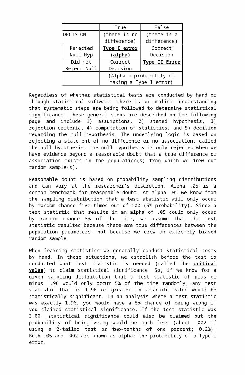
reasonable doubt that a true difference or association exists in the population(s) from which we drew our random sample(s).

Reasonable doubt is based on probability sampling distributions and can vary at the researcher's discretion. Alpha .05 is a common benchmark for reasonable doubt. At alpha .05 we know from the sampling distribution that a test statistic will only occur by random chance five times out of 100 (5% probability). Since a test statistic that results in an alpha of .05 could only occur by random chance 5% of the time, we assume that the test statistic resulted because there are true differences between the population parameters, not because we drew an extremely biased random sample.

When learning statistics we generally conduct statistical tests by hand. In these situations, we establish before the test is conducted what test statistic is needed (called the critical value) to claim statistical significance. So, if we know for a given sampling distribution that a test statistic of plus or minus 1.96 would only occur 5% of the time randomly, any test statistic that is 1.96 or greater in absolute value would be statistically significant. In an analysis where a test statistic was exactly 1.96, you would have a 5% chance of being wrong if you claimed statistical significance. If the test statistic was 3.00, statistical significance could also be claimed but the probability of being wrong would be much less (about .002 if using a 2-tailed test or two-tenths of one percent; 0.2%). Both .05 and .002 are known as alpha; the probability of a Type I error.

When conducting statistical tests with computer software, the exact probability of a Type I error is calculated. It is presented in several formats but is most commonly reported as "p <" or "Sig." or "Signif." or "Significance." Using "p <" as an example, if a priori you established a threshold for statistical significance at alpha .05, any test statistic with significance at or less than .05 would be considered statistically significant and you would be required to reject the null hypothesis of no difference. The following table links p values with a benchmark alpha of .05:  

P < Alpha Probability of Type I Error Final Decision.05 .05 5% chance difference is not

significantStatistically significant

.10 .05 10% chance difference is not significant

Not statistically significant

.01 .05 1% chance difference is not significant

Statistically significant

.96 .05 96% chance difference is not significant

Not statistically significant

Steps to Hypothesis Testing

Hypothesis testing is used to establish whether the differences exhibited by random samples can be inferred to the populations from which the samples originated.

General Assumptions

Population is normally distributed Random sampling Mutually exclusive comparison samples Data characteristics match statistical technique

For interval / ratio data use   t-tests, Pearson correlation, ANOVA, regression

 For nominal / ordinal data use  

Difference of proportions, chi square and related measures of association

State the Hypothesis

Null Hypothesis (Ho): There is no difference between ___ and ___.

Alternative Hypothesis (Ha): There is a difference between __ and __.

Note: The alternative hypothesis will indicate whether a 1-tailed or a 2-tailed test is utilized to reject the null hypothesis.

Ha for 1-tail tested: The __ of __ is greater (or less) than the __ of __.

Set the Rejection Criteria This determines how different the parameters and/or statistics must be before the null hypothesis can be rejected. This "region of rejection" is based on alpha ( ) -- the error associated with the confidence level. The point of rejection is known as the critical value.

Compute the Test Statistic The collected data are converted into standardized scores for comparison with the critical value.

Decide Results of Null Hypothesis If the test statistic equals or exceeds the region of rejection bracketed by the critical value(s), the null hypothesis is rejected. In other words, the chance that the difference exhibited between the sample statistics is due to sampling error is remote--there is an actual difference in the population.

Let us consider an experiment involving two groups, an experimental group and a control group. The experimenter likes to test whether the treatment (values clarification lessons) will improve the self-concept of the experimental group. The same treatment is not given to the control group. It is presumed that any difference between the two groups after the treatment can be attributed to the experimental treatment with a certain degree of confidence.

The hypothesis for this experiment can be stated in various ways:

a) No existence or existence of a difference between groups

Ho: There is no significant difference in self-concept between the group exposed to values clarification lessons and the group not exposed to the same.

Ha: The self-concept of the group exposed to values clarification lessons differ significantly that of the other group.

b) No existence or existence of an effect of the treatment

Ho: There is no significant effect of the values clarification lessons on the self-concept of the students. Ha: Values clarification lessons have no significant effect on the self-concept of students.

c) No existence of relationship between the variablesHo: The self-concept of the students is not significantly related to the values

clarification lessons conducted on them.

Ha: The self-concept of the students is not significantly related to the values clarification lessons they were exposed to.

Parametric Test

What are the parametric tests?

The parametric tests are tests that require normal distribution, the levels of measurement of which are expressed in an interval or ratio data. The following parametric tests are:

t-test for one population mean compared to a sample mean

t- test for Independent Samples

t- test for Correlated Samples

z- test, for Two Sample Means

z- test for One Sample Group

F- test (ANOVA)

R (Pearson Product Moment Coefficient of Correlation)

Y=a+bx (Simple Linear Regression Analysis)

Y=b0+b1 x1+b2 x2+... +bn xn

(Multiple Regression Analysis)

Comparing a Population Mean to a Sample Mean (T-test)

Example 1: Compare the mean age of incoming students to the known mean age for all previous incoming students. A random sample of 30 incoming college freshmen revealed the following statistics: mean age 19.5 years, standard deviation 1 year. The college database shows the mean age for previous incoming students was 18.

Solving by the Stepwise Method

I. Problem: Is there a significant difference between the mean age of past college students and the mean age of current incoming college students?

II. Hypothesis

Ho: There is no significant difference between the mean age of past college students and the mean age of current incoming college students.

Ho: x1=x2

Ha: There is a significant difference between the mean age of past college students and the mean age of current incoming college students.

III. Level of Significance

Set the Rejection Criteria Significance level .05 alpha, 2-tailed test Degrees of Freedom = n-1 or 29 Critical value from t-distribution = 2.045

IV. Statistics

Compute the Test Statistic

t=x− ¿s

√n−1

¿

t=19.5−181

√30−1

t= 1.51

√29

t= 1.5.186

t = 8.065

V. Decision Rule: If the t- computed value is greater than or beyond the t-tabular / critical value, reject H 0.

VI Conclusion: Given that the test statistic (8.065) exceeds the critical value (2.045), the null hypothesis is rejected in favor of the alternative. There is a statistically significant difference between the mean age of the current class of incoming students and the mean age of freshman students from past years. In other words, this year's freshman class is on average older than freshmen from prior years.

If the results had not been significant, the null hypothesis would not have been rejected. This would be interpreted as the following: There is insufficient evidence to conclude there is a statistically significant difference in the ages of current and past freshman students.

What is the t-test for independent samples?

The t-test is a test of difference between two independent groups. The means are being compared x1 againstx2.

When do we use the t-test for independent samples?

The t-test for independent samples is used when we compare means of two independent groups.

When the distribution is normally distributed, Sk = 0 and Ku = .265.we use interval or ratio data.

the sample is less than 30.

Why do we use the t-test for independent sample?

The t-test is used for independent sample because it is more powerful test compared with other tests of difference of two independent groups.

How do we use the t-test for independent samples?

t = x1− x2

√¿¿¿Where:

t = the t testx1= the mean of group 1

x2 = the mean of group 2 SS1 = the sum of squares of group 1 SS2 = the sum of squares of group 2 n1 = the number of observations in group 1 n2 = the number of observations in group 2

or

t = x1− x2

√¿¿¿Where:Typeequationhere .

t = the t testx1= the mean of group 1 or sample 1

x2 = the mean of group 2 or sample 2 S1 = the standard deviation of group 1 or sample 1 S2 = the standard deviation of group 2 or sample 2 n1 = the number of observations in group 1 n2 = the number of observations in group 2

Example 1. The following are the scores of 10 male and 10 female AB students in spelling. Test the null hypothesis that there is no significant difference between the performance of male and female AB students in the rest. Use the t-test .05 level of significance.

Male (x1) Female (x2) 14 12 18 9 17 11 16 5 4 10 14 3 12 7 10 2 9 6 17 13

Solution:Male Female

x1 x21

x2 x22

14 196 12 144 18 324 9 81 17 289 11 121 16 256 5 25 4 16 10 100 14 196 3 9 12 144 7 49 10 100 2 4 9 81 6 36 17 289 13 169 ______ _______ _______ _______ ∑ x1 =131 X1

2 = 1891 ∑ x2=78 X22 = 738

n1 = 10 n2 = 10 x1 = 13.1 x2= 7.8

t = x1− x2

√¿¿¿

t = 13.1−7.8

√[ 174.9+129.610+10−2 ][ 1

10+ 1

10 ]

t = 5.3

√[ 304.518 ](.1+.1)

t = 5.3

√(16.92 ) ( .2 )

t = 5.3

√3.384

t = 5.3

1.8395

t = 2.88

Solving by the Stepwise Method

I. Problem:Is there a significant difference between the performance of the male and female students in spelling?

II. Hypothesis:

H 0 : There is no significant difference between the performance of the male and the female AB students in spelling.

H 0 : x1=x2 H a : There is a significant difference between the performance of the

male and the female AB students in spelling. H a : x1=x2

III. Level of Significance:α=.05

df = n1+n2- 2 = 10 + 10 – 2 = 18

t..05 = 2.101 t-tabular value at .05

IV. Statistics: t-test for two independent Samples

V. Decision Rule: If the t- computed value is greater than or beyond the t- tabular / critical value, reject H 0.

VI. Conclusion:Since the t-computed value of 2.88 is greater than t-tabular value of 2.101 at .05 level of significance with 18 degrees of freedom, the null hypothesis is rejected in favor of the research hypothesis. This means that there is a significant difference between the performance of the male and female AB students in spelling, implying that the male students performed better than the female students considering that the mean/average score of the male students of 13.1 is greater compared to the average score of female students of only 7.8.

Example 2.

Two groups of experimental rats were injected with tranquilizer at 1.0 mg. And 1.5 mg dose respectively. The time given in seconds that took them to fall asleep in hereby given. Use the t-test for independent samples at .01 to test null hypothesis that the difference in dosage has no effect on the length of time it took them to fall asleep.

1.0 mg dose: 9.8, 13.2, 11.2, 9.5, 13.0, 12.1, 9.8, 12.3, 7.9, 10.2, 9.7.1.5 mg dose: 12.0, 7.4, 9.8, 11.5, 13.0, 12.5, 9.8, 10.5, 13.5.

Solution:

(1.0 mg dose) (1.5 mg dose)

X1 X1

2 X2 X2

2

9.8 96.04 12.0 144.00 13.2 174.24 7.4 54.76 11.2 125.44 9.8 96.04 9.5 90.25 11.5 132.25 13.0 169.00 13.0 169.00 12.1 146.41 12.5 156.25 9.8 96.04 9.8 96.04 12.3 151.29 10.5 110.25 7.9 62.41 13.5 182.25 10.2 104.04 X2 =100 X2

2 = 1140.84 9.7 94.09 n2= 9 X1 = 118.7 x1=11.11 X1

2 =1309.25

N1 = 11 X1 =10.79

SS1 = - X1−¿2¿ (∑ x1¿

2

n1

SS2 = X22 -

(∑ x2¿2

n2

= 1309.25- ¿¿ = 1140.84 –¿¿SS1 = SS2=

t= x1− x2

√¿¿¿

= 10.79−11.11

√[ 28.37+29.7311+9−2 ] [ 1

11+ 1

9 ]

= −0 .32

√[ 58 .1018 ](.09+.11)

= −0 .32

√(3 .23 )( .2)

=−0 .32

√.646

= −0 .32.8037

t = -0.40

Solving by the Stepwise Method

I. Problem : Is there a significant difference brought about by the dosages on the length of time it took for the rats to fall asleep

II. Hypothesis: H 0 : There is no significant differences brought about by the dosages on the length of time it took the rats to fall asleep.

H a : There is a significant difference brought about by the dosages on the length of time it took for the rats to fall asleep.

III. Level of Significance:

α=.01 df = n1+n2- 2

= 11 + 9 – 2 = 18

t.05 = -2.88 IV. Statistics: t-test for two independent samples

V. Decision Rule: If the t- computed value is greater than or beyond the t-tabular / critical value, reject H 0.

VI. Conclusion: Since the t-computed value of /-.40/ is within the critical value of /-2.88/ at .01 level of significance with 18 degrees of freedom, the

28.37 29.73

null hypothesis is not rejected. This means that no significant difference was brought about by the dosages on the length of time it took for the rats to fall asleep.

Example 3. To find out whether a new serum would arrest leukemia, 16 patients on the advanced stage of the disease were selected. Eight patients received the treatment and eight did not. The survival was taken from the time the experiment was conducted.

No treatment With Treatment X1

X12 X2 X2

2

2.1 4.41 4.2 17.64

3.2 10.24 5.1 26.01

3.0 9.00 5.0 25.00

2.8 7.84 4.6 21.16

2.1 4.41 3.9 15.21

1.2 1.44 4.3 18.49

1.8 3.24 5.2 27.04

1.9 3.61 3.9 15.21

∑ x1 = 18.1 X12= 44.19 ∑ x2 = 362 X2

2 = 165.76 n1 = 8 n2 = 8 x1 = 2.2 x2= 4.52

Solution: Solve for ∑ x1 , X12and x1 likewise for ∑ x2, X2

2 and x2 . Then solve for the sum of the squares of group 1, and sum of squares of group 2 SS1 and SS2 .

SS1 = - X12-

(∑ x1¿2

n1

SS2 = X22 -

(∑ x2¿2

n2

= 44.19 - ¿¿ = 165.76 – ¿¿ = 44.19 – 40.95 =165.76 – 163.80 SS1=¿ == SS2= 1.96

t = x1− x2

√¿¿¿

= 2.26−4.52

√[ 3 .24+1 .968+8−2 ][ 1

8+ 1

8 ]

= −2.26

√[ 5.214 ][ 2

8 ]

= −2.26

√( .37 ) ( .25 )

= −2.26

√.0925

= −2.26.3041

3.24

t = -7.43

Solving by the Stepwise Method

I. Problem: Will the new serum arrest leukemia for the 8 patients who had reached the advanced stage?

II. Hypothesis:

H 0 : The new serum will not arrest the leukemia of the 8 patients who had reached the advanced stage of the disease.

H 1 : The new serum will arrest the leukemia of the 8 patients who had reached an advanced stage of the disease.

III. Level of Significance:α=.05

df = n1+n2- 2 = 8 + 8 – 2 = 14

t.05 = -2.145

IV. Statistics: t-test for independent samples

V. Decision Rule: If the t-computed value is greater than or beyond the critical or tabular value, reject H 0.

VI. Conclusions: The t-computed value is /-7.43/ which is beyond the critical value of /-2.145/ at .05 level of significance with 14 degrees of freedom. The null hypothesis therefore is disconfirmed in favor of the research hypothesis. This means that the new serum will arrest the advanced stage of leukemia.

What is the t-test correlated samples?

The t-test for correlated samples is another parametric test applied to one group of samples. It can be used in the evaluation of a certain program or treatment. Since this is another parametric test, conditions must be met like the normal distribution and the use of interval or ratio data.

When do we use the t-test for correlated samples?

The test for correlated samples is applied when the mean before and the mean after are being compared. The pretest (mean before) is measured, the treatment of the intervention is applied and then the posttest (mean after) is likewise measured. Then the two means (pretest vs. the posttest) are compared.

Why do we use the t-test for correlated samples?

The t-test for correlated samples is used to find out if a difference exists between the before and after means. If there is a difference in favor of the posttest then the treatment or intervention is effective. However, if there is no significant difference then the treatment is not effective.

This is the appropriate test for evaluation of government programs. This is used in an experimental design to test the effectiveness of a certain technique or method or program that had been developed.

How do we use the t-test for correlated samples?

The formula is

t= D

√D2−¿¿¿¿

Where: D= the eman difference between the pretest and the posttest.

D2= the sum of the squares of the difference between the pretest and the posttest.

D = the summation of the difference between the pretest and the posttest.

n = the sample size

Example 1. An experiment study was conducted on the effect of programmed materials in English on the performance of 20 selected college students. Before the program was implemented the pretest was administered and after 5 months the same instrument was used to get the posttest result. The following is the result of the experiment. Use αat .05 level.

Pretest PosttestX1

X12 D D2

20 25 -5 2530 35 -5 2510 25 -15 22515 25 -10 10020 20 0 010 20 -10 10018 22 -4 1614 20 -6 3615 20 -5 2520 15 5 2518 30 -12 14415 10 5 2520 25 -5 118 10 8 6440 45 -5 2510 15 -5 2510 10 0 012 18 -6 3620 25 -5 25

_____________ ______________

D = -81 D2 = 94

D= −8120

D = - 4.05

What are the steps in using the t-test for correlated samples?

Subtract the difference between the two observations before and after the treatment.

Find the summation of the difference algebraically D (consider the + and – sign)

Compute D the mean difference, D n

Square the difference between the before and after observation and get the summation that is D2

Determine the number of observation that is small letter n.

If the t-compound value is greater than or beyond the critical value disconfirm the null hypothesis and confirm the research or alternative hypothesis.

t = D

√D2−¿¿¿¿

= −4.05

√947−¿¿¿¿

= −4.05

√ 947−328.0520(19)

= −4.05

√ 618.95380

= −4.05

√1.6288

= −4.051.2762

t = -3.17

Solving by the Stepwise Method

I. Problem: Is there a significant difference between the pretest and the posttest on the use of programmed materials in English?

II. Hypotheses:

H 0 : There is no significant difference between the pretest and the posttest, or the use of the programmed materials did not affect the students’ performance in English.

H 1 : The posttest result is higher than the pretest result.

III. Level of Significance:

α=.05 df = n-1

= 20-1 = 14

t.05 = -1.729

IV. Statistics: t-test for correlated samples

V. Decision Rule: If the t-computed value is greater than orbeyond the critical value, reject H 0.

VI. Conclusion: The t-compound value of 3.17 is beyond the t-critical valueof /-1.73/ at .05 level of significance with 19 degrees of freedom. The null hypothesis is therefore rejected in favor of the research hypothesis. This means that the posttest result is higher than the pretest result. It implies that the use of the programmed materials in English is effective.

What is the z-test?

The z-test is another test under parametric statistics which requires normality of distribution. It uses the two population parameters and .

It is used to compare two means, the sample mean, and the perceived population mean.

It is also used to compare the two sample means taken from the same population. It is used when the samples are equal to or greater than 30. The z-test can be applied in two ways: the One-Sample Mean Test and the Two-Sample Mean Test.

The tabular value of the z-test at .01 and .05 level of significance is shown below.

Test Level of Significance

.01 .05

One-tailed ± 2.33 ± 1.645

Two-tailed ± 2.575 ± 1.96

What is the z-test for one sample group?

The z-test for one sample group is used to compare the perceived population mean against the sample mean, X

When is the z-test for a one-sample group?

The one-sample group test is used when the sample is being compared to the perceived population mean. However if the population standard deviation is not known the sample standard deviation can be used as a substitute.

Why is the z-test used for a one-sample group?

The z-test is used for a one-sample group because this is appropriate for comparing the perceived population mean against the sample mean X . We are interested if significant difference exists between the population against the sample mean. For instance a certain tire company would claim that the life span

odd its product will last 25,000 kilometers. To check the claim, sample tires will be tested by getting sample mean X .

How do we use the z-test for a one-sample group?

The formula is

z = ¿¿ Where:

X = sample mean = hypothesized value of the population mean = population standard deviation N = sample size

Example 1. The ABC company claims that the average lifetime of a certain tire as at least 28,000 km. To check the claim, a taxi company puts 40 of these tires on its taxis and gets a mean lifetime of 25,560 km. With a standard deviation of 1,350 km, is the claim true? Use the z-test at .05.

What are the steps in using the z-test for a one sample group?

Solve for the mean of the sample and also the standard deviation if the population is not known.

Subtract the population from the sample mean and multiply it by the square root of n sample.

Divide the result from step 2 by the population standard deviation on the sample standard deviation if the population is not known.

Compare the result in the table of the tabular value of the z-test at .01 and .05 level of significance.

Level of Significance Test .01 .05 One tailed ± 2.33 ± 1.645 Two tailed ± 2.575 ± 1.96ɑɑ

If the z-compound value is greater than or beyond the critical value, reject the null hypothesis and confirm the research hypothesis.

I. Problem: Is the claim true that the average lifetime of a certain tire is at least 28,000 km?

II. Hypotheses:

H 0 : The average lifetime of a certain tire is 28,000 km.

H 1 : The average lifetime of a certain tire is not 28,000 km.

III. Level of Significance:

ɑ = .05 z = ±1.645

IV. Statistics:

z-test for a one-tailed test

Computation: _

z = ¿¿

= (25,560−28,000)√401,350

=(−2,440)(6.32)

1,350

= −15,420.8

1,350

z = -11.42

V. Decision Rule: if the z computed is greater than or beyond the z tabular value, reject the Ho.

VI. Conclusion: Since the z computed of -11.42 is beyond the critical value of -1.645 at .05 level of significance the research hypothesis is rejected which means that the average lifetime of a certain tire is not 28,000 km.

What is the z-test for a two-sample mean test?

The z-test for a two-sample mean test is another parametric test used to compare the means of two independent groups of samples drawn from a normal population if there are more than 30 samples for every group.

When do we use the z-test for two sample mean?

The z-test for two-sample mean is used when we compare the means of samples of independent groups taken from a normal population.

Why do we use the z-test?

The z-test is used to find out if there is a significant difference between the two populations by only comparing the sample mean of the population.

How do we use the z-test for a two-sample mean test?

The formula is

z = x1−x2

√ s12

n1

+s2

2

n2

where:

x1 = the mean of sample 1 x2 = the mean of sample 2 s1

2 = the variance of sample 1

s22 = the variance of sample 2

n1 = size of sample 1 n2 = size of sample 2

Example 1. An admission test was administered to incoming freshmen in the colleges of Nursing and Veterinary Medicine with 100 students each college randomly selected. The mean scores of the given samples where x1= 90 and x2= 85 and the variances of the test scores were 40 and 35 respectively. Is there a significant difference between the two groups? Use .01 level of significance.

What are the steps in solving for the z-test for two-sample mean?

Compute the sample mean of group 1, x1 and also the sample mean of group 2, x2

Compute the standard deviation of group 1 SD1 and standard deviation of group 2 SD2.

Square the SD1 of group 1 to get the variance of group 1 s12 and also square the

SD2 of the group 2 to get the variance of group 2 s22.

Determine the number of observation in group 1 n1 and also the number of observation in group 2 n2.

Compare the z computed value from the z- tabular value at certain level of significance.

Level of Significance

Test .01 .05 One-tailed ± 2.33 ± 1.645 Two-tailed ± 2.575 ± 1.96

If the computed z-value is greater than or beyond the critical value reject the null hypothesis and do not reject the research hypothesis.

I. Problem: Is there a significant difference between the two groups?

II. Hypotheses: H 0 : x1=x2

H 1 : x1≠ x2

III. Level of Significance

α = .01

z = ± 2.575

do not reject H 0

reject H 0

reject H 0

-2.575 -1 0 +1 0+2.575

-1.96 +1.96IV. Statistics: z-test for two-tailed test

z = x1−x2

√ s12

n1

+s2

2

n2

¿ 90−85

√ 40100

+ 35100

= 5

√ 75100

= 5

√.75

= 5

.866

z = 5.774

V. Decision Rule: If the z-computed value is greater than or beyond the z =tabular value, reject the null hypothesis..

VI. Conclusion: Since the z-computed value of 5.774 is greater than the z-tabular value of 2.575 at .01 level of significance, the research hypothesis is rejected which means that there is a significant difference between the two groups. It implies that the incoming freshmen of the College of Nursing are better than the incoming freshmen of the College of Veterinary Medicine.

What is the F-test?

The F-test is another parametric test used to compare the means of two or more groups of independent samples. It is also known as the analysis of variance, (ANOVA).

The three kinds of analysis of variance are:

one-way analysis of variance

two-way analysis of variance

three-way analysis of variance

The F-test is the analysis of variance (ANOVA). This is used in comparing the means of two or more independent groups. One-way ANOVA is used when there is only one variable involved. The two-way ANOVA is used when two variables are involved: the column and the row variables. The researcher is interested to know if there are significant differences between and among columns and rows. This is also used in looking at the interaction effect between the variables being analyzed.

Like the t-test, the F-test is also a parametric test which has to meet some conditions, and the data to be analyzed if they are normal are expressed in interval or ratio data. This test is more efficient than other tests of difference.

Why do we use the F-test?

The F-test is used to find out if there is a significant difference between and among the means of the two or more independent groups.

When do we use F-test?

The F-test is used when there is normal distribution and when the level of measurement is expressed in interval or ratio data just like the t-test and the z-test.

How do we use the F-test?

To get the F computed value, the following computations should be done.

CF=(¿)2

N

TSS is the total sum of squares minus the CF, the correction factor.

BSS is the between sum of squares minus the CF correction factor.

WSS is the sum of squares or it is the difference between the TSS minus BSS.

After getting the TSS, BSS and WSS, the ANOVA table should be constructed.

ANOVA TableSources of F-Value

Df SS MS Computed Tabular

Between K-1 BSS BSSdf

MSBMSW

=F see the table

at .05 or the

desired level

of significance

Within (N-1)-(K-1) WSS WSSdf

w/ df between

Group and w/ groupTotal N-1 TSS

What are the steps in solving for the F-value?

The ANOVA table has five columns. These are:sources of variations, degrees of freedom, sum of squares, mean squares and the F-value, both the computed and the tabular values.

The sources of variations are between the groups, within the group itself and the total variations.

The degrees of freedom for the total is the total number of observation minus 1.

The degrees of freedom from the between group is the total number of groups minus 1.

The degrees of freedom for the within group is the total df minus the between groups df.

The MSB mean squares between is equal to the BSS/df.

The MSW mean square within is equal to the WSS/df.

To get the F-computed value, divide MSB/MSW.

If the F-computed value at a given level of significance with the corresponding df’s of BSS and WSS.

If the F computed value is greater than the F-tabular value, reject the null hypothesis in favour of the research hypothesis.

When the F-computed value is greater than the F-tabular value the null is rejected and the research hypothesis not rejected which means that there is a significant difference between and among the means of the different groups.

Example 1: A sari-sari store is selling 4 brands of shampoo. The owner is interested if there is a significant difference in the average sales of the four brands of shampoo for one week. The following data are recorded.

Brand

A B C D 7 9 2 4 3 8 3 5 5 8 4 7 6 7 5 8 9 6 6 3 4 9 4 4 3 10 2 5

Perform the analysis of variance and test the hypothesis at .05 level of significance that the average sales of the four brands of shampoo are equal.

Solving by the Stepwise Method

I. Problem: Is there a significant difference in the average sales of the four brands of shampoo?

II. Hypotheses:

H 0 : There is no significant difference in the average sales of the four brands of

shampoo H 1 : There is a significant difference in the average sales of the four brands of

shampoo.

CF=❑1+❑2+❑3+❑4

n1n2n3n4

=¿¿

TSS = x12+ x2

2+x32+x4

2−CF

= 225+475+110+204-869.14

=1014 – 869.14

TSS = 144.86BSS = ¿¿

= ¿¿ = 195.57+464.14+96.57+185.14-869.14 = 941.42-869.14

BSS = 72.28

WSS = TSS – BSS

=144.86 – 72.28WSS = 72.58

Analysis of Various Table

F-Value Sources of Degrees of Sum of Mean Variation Freedom Squares Squares _______________

Computed Tabular

Between Groups K-1 3 72.28 24.09 7.98 3.01 Within Group (N-1)-(K-1) 24 72.58 3.02Total N-1 27 144.86

III. Decision Rule: If the F computed value is greater than the F-tabular value, reject H 0.

IV. Conclusion: Since the F-computed value of 7.98 is greater than the F –tabular value of 3.01 at .05 level of significance with 3 and 24 degrees of freedom, the null hypothesis is rejected in favor of the research hypothesis which means that there is a significant difference in the average sales of the 4 brands of shampoo.

What is the Scheffe’s Test?

To find out where the differences lies, another test must be used.

The F-test tells us that there is a significant difference in the average sales of the 4 brands of shampoo but as to where the difference lies, it has to be tested further by another test, the Scheffe’s test formula.

F '=¿¿

Where: F ' = Scheffe’s test x1 = mean of group 1 x2 = mean of group 2 n1 = number of samples in group 1 n2 = number of samples in group 2 SW 2 = within mean squares

A vs. B

F '=¿¿

¿ 8.1796

42.2849

¿8.1796

.86

F ' =

A vs C A vs D

F '=¿ ¿¿ F '=¿ ¿¿

=2.4649

.86 =.0196

.86

F '=¿ F '=¿

9.51

2.87 .02

B vs C B vs D

F '=¿ ¿¿ F '=¿ ¿¿

=19.6249

.86 =9

.86

F '=¿ F '=¿

C vs D

F '=¿ ¿¿

=2.0449

.86

F '=¿

Comparison of the Average Sales of the Four Brands of Shampoo

Between F ' (F .05 ) Brand (K−1 ) Interpretation (3.01 ) (3 )

A vs B 9.51 9.03 significant A vs C 2.87 9.03 not significant A vs D .02 9.03 not significant B vs C 22.82 9.03 significant B vs D 10.46 9.03 significant C vs D 2.38 9.03 not significant

The above table shows that there is a significant difference in the sales between brand A and brand B, brand B and brand C and also brand B and D. However, brands A and C, A and D and C and D not significantly differ in their average sales.

This implies that brand B is more saleable than brands A, C and D.

Example 2. The following data represent the operating time in hours of the 3 types of scientific pocket calculators before a recharge is required. Determine the difference in the operating time of the three calculators. Do the analysis of variance at .05 level of significance.

BrandFx1

X12 Fx2

X22 Fx3

X32

4.9 24.01 6.4 40.96 4.8 23.045.3 28.09 6.8 46.24 5.4 29.164.6 21.16 5.6 31.36 6.7 44.896.1 37.21 6.5 42.25 7.9 62.414.3 18.49 6.3 39.69 6.2 38.446.9 47.61 6.7 44.89 5.3 28.09 5.3 28.09 5.9 34.81 4.1 16.81 4.3 18.49

22.82 10.46

2.38

x1= 32.1 x12=176.57 x2= 52 x2

2 = 308.78 x3 =42.2 x32 = 260.84

n1= 6 n2 = 9 n3= 7x1 = 5.35 x2 = 5.78 x3 = 6.03

I. Problem: Is there a significant difference in the average operating time in hours of the 3 types of pocket scientific calculators before a recharge is required?

II. Hypotheses:

H 0 : There is no significant difference in the average operating time in hours

among the 3 types of pocket calculators before a recharge is required.

H 1 : There is a significant difference in the average operating time in hours of the 3 types of pocket scientific calculators before a recharge is required.

III. Level of Significance:α = .05df = 2 and 19

IV. Statistics:F-test one-way-analysis of variance

Computation:

CF = ¿¿ = 725.08

TSS = x12+ x2

2+x32 – CF

= 176.57+308.78+260.78+260.84-725.08 = 746.19 – 725.08TSS =

BSS = ¿¿ = ¿¿ - 725.08 =171.74+300.44+254.40-725.08 = 726.58-725.08

BSS =

WSS = TSS-BSS = 21.11 – 1.50WSS = 19.61

ANOVA TABLE

Sources of Degrees Sum of Mean ComputedVariation of Freedom Squares Squares F-Value Tabular

Between Groups K-1 2 1.50 .75 .73 3.52

Within Group (N-1)-(K-1) 19 19.61 1.03

21.11

1.50

Total N-1 21 21.11

V. Decision Rule: If the F-computed value is greater than the F-tabular value, reject the H 0.

VI. Conclusion: Since the F-computed value of 0.73 is lesser than the F-tabular value of 3.52 at .05 level of significance, the null hypothesis is not rejected. This means that there is no significant difference in the average operating time in hours of the 3 types of pocket scientific calculators before a recharge is required.

What is the F-test two-way-ANOVA with interaction effect?

The F-test, two-way-ANOVA involves two variables, the column and the row variables.

It is used to find out if there is an interaction effect between two variables.

How do you use the F-test two-way-ANOVA with interaction effect?

Consider this example

Example 1. Forty-five language students were randomly assigned to one of three instructors and to one of the three methods of teaching then achievement was measured on a test administered at the end of the term. Use the two-way ANOVA with interaction effect at .05 level of significance to test the following hypotheses:

1. H 0: There is no significant difference in the performance of the three groups of students under three different instructors.

H 1: There is a significant difference in the performance of the three groups of students under three different instructors.

2. H 0: There is no significant difference in the performance of the three groups of students under three different methods of teaching.

H 1: There is a significant difference in the performance of the three groups of students under three different methods of teaching.

3. H 0: Interaction effects are not present.H 1: Interaction effects are present.

TWO-FACTOR ANOVA with a significant InteractionTEACHER FACTOR

A B C

Methods of Teaching 1

40 50 4041 50 4140 48 4039 48 3838 45 38

Total

Method of teaching 2

40 45 5041 42 4639 42 4338 41 4338 40 42

Total

Method of Teaching 3

40 40 4043 45 4141 44 4139 44 3938 43 38

TotalTotal

Solving by the Stepwise Method

I. Problem: 1. Is there a significant difference in the performance of students under the three different teachers?

2. Is there a significant difference in the performance of students under the three different methods of teaching?

3. Is there an interaction effect between teacher and method of teaching factors?

II. Hypotheses:

1. H 0: There is no significant difference in the performance of the three groups of students under three different instructors.

H 1: There is a significant difference in the performance of the three groups of students under three different instructors.

2. H 0: There is no significant difference in the performance of the three groups of students under three different methods of teaching.

H 1: There is a significant difference in the performance of the three groups of students under three different methods of teaching.

3. H 0: Interaction effects are not present. H 1: Interaction effects are present.III. Level of Significance

a = .05 df total = N-1 df within = k(n-1) df column = c-1 df row = r-1 df c ° r = (c-1)(r-1)

IV. Statistics: F-test Two-Way-ANOVA with interaction effect

TWO-FACTOR ANOVA with Significant Interaction TEACHER FACTOR (Column)

A B C

Method of Teaching

FACTOR 1 (row)

40 50 4041 50 4140 48 4039 48 3838 45 38

Total 198 241 197 = 636

Method of Teaching

FACTOR 2 (row)

40 45 5041 42 4639 42 4338 41 4338 40 42

Total 196 210 224 = 630

Method of Teaching

FACTOR 3(row)

40 40 4043 45 4131 44 4139 44 3938 43 38

Total 201 216 199 =616Total 595 667 620 =

1882

CF = ¿¿ = 78709.42

SST= 402+412+…+392+382- CF

= 79218-78709.42

= 508.58

SSw = 79218- ¿¿ ¿¿ = 79218 – 79088.8 = 129.2SSc = ¿¿ - CF

= 1183314

15 -78709.42

= 178.18SSr=¿¿ – CF

= 1180852

15 -78709.42

= 787.723.47 – 78709.42 =14.05SSc r=SS t−SSw−SSc−SSr = 508.58 – 129.2 – 178.18 – 14.05

= 187.15

The degrees of freedom for the different parts of the problem are:df t = N-1 = 45-1 = 44df w = k(n-1) = 9(5-1) = 9(4) = 36 df c = (c-1) = (3-1) = 2

df r = (r-1) = (3-1) = 2df c∗r = (c-1)(r-1) = (3-1)(3-1) = (2)(2) = 4

ANOVA TABLE

Sources ofVariation

SS df MS

F-valueComputed

Tabular Interpretation

BetweenColumns

178.18 2 89.9 24.82 3.26 SRows 14.05 4 7.02 1.95 3.26 NSInteraction

187.15 4 46.79 13.03 2.63 S

Within 129.20 36 3.59Total 508.58 44

F-Value Computed:

Columns = MScMSw

=89.093.59

= 24.82

Row = MSRMSw

=7.023.59

= 1.95

Interaction = MSIMSw

=46.793.59

= 13.03

F-Value Tabular at .05

Columns df = 2/36 = 3.26

Row df = 2/36 = 3.26Interaction df = 4/36 = 2.63

V. Decision Rule: If the computed F value is greater than the F critical/tabular value, reject H 0.

VI. Conclusion: With the computed F-value (column) of 24.82 compared to the F-tabular value of 3.26 at .05 level of significance with 2 and 36 degrees of freedom, the null hypothesis is rejected in favor of the of the research hypothesis which means that there is a significant difference in the performance of the three groups of students under three different instructors. It implies that instructor B is better than instructor A. With regard to the F-value (row) of 1.95, it is lesser than the F-tabular value of 3.26 at .05 level of significance with 2 and 36 degrees of freedom. Hence, the null hypothesis of no significant differences in the performance of the students under the three different methods of teaching is not rejected.

However, the F-value (interaction) of 13.03 is greater than the F-tabular value of

2.63 at .05 level of significance with 4 and 36 degrees of freedom. Thus, the research hypothesis is rejected which means that interaction effect is present between the instructors and their methods of teaching. Students under instructor B have better performance under methods of teaching 1 and 3 while students under instructor C have better performance under method 2.

What is the Pearson Product Moment Coefficient of Correlation r?

The Pearson Product Moment Coefficient of Correlation r is an index of relationship between two variables. The independent variable can be represented by x while the dependent variable can also be represented by y. The value of r is +1, zero to -1. If the value of r is +1 or -1, there is a perfect correlation between x and y. However, if r equals zero then x and y are independent of each other.

Consider the x and y coordinates in the graph below.y

High

r = +

xLow High

If the trend of the line graph is going upward, the value of r is positive. This indicates that as the value of x increase the value of y also increase. Likewise, if the value of x decreases, the value of y also decreases, the x and y being positively correlated.

yHigh

r = ___

XLow High

If the trend of the line graph is going downward, the value of r is negative. It indicates that as the value of x increases the corresponding value of y decreases, x and y being negatively correlated.

y

Highr = 0

x Low High

If the trend of the line graph cannot be established either upward or downward, then r = 0, indicating that there is no correlation between the x and y variables.

Why do we use r?

We use r because we want to analyze if a relationship exists between two variables. If there is a relationship that exists between the x and y, then we can determine the extent by which x influences using the coefficient of determination which is equal to the square of r and multiplied by 100%. This can answer or explain how much the independent variable influences the dependent variables or how much y depends on x. This is now the degree of relationship between x and y which can not be seen in other statistical tests of relationship.

We also use r because it is a more powerful test of relationship compared with other nonparametric tests.

When do we use r, the Pearson Product Moment Coefficient of Correlation?

We use the r to determine the index of relationship between two variables, the independent and the dependent variables. If there is relationship between the independent and the dependent variables, we can say that x influences y or y depends on x. however if there is no relationship that exists between x and y then x and y are independent of each other.

The value of r ranges from +1 through zero -1. There is a perfect positive correlation of r = +1, likewise there is a negative perfect correlation if the value of r = -1. However if r = 0 then there is no correlation between the two variables x and y. If there is a positive correlation it indicates that for every increase of y or for every decrease of x there is a corresponding decrease of y. If there is a negative correlation it indicates that for every increase of x there is a corresponding decrease of y, likewise for every decrease of x there is a corresponding decrease of y, likewise for every decrease of x there is a corresponding increase of y. The relationship is inverse.

How do we use r Pearson Product Moment Coefficient Correlation?

The Pearson Product Moment Coefficient of Correlation represented by small letter r is determined by using the formula

r = n xy−x y

√nx2−¿¿¿

Where:r = the Pearson Product Moment Coefficient of Correlationn = sample size

xy = the sum of the product of x and y x y = the product of the sum of x and the sum of

y x2 = sum of squares of x y2 = sum of squares of y

Example 1. Below are the midterm (x) and final (y) grades.

x 75 7065 90 85 8580 70 65 90y80 75 65 95 90 85 90 75 70 90

What are the steps in solving for the value of r?

Determine the number of observation n.

Get the sum of x that is x, the independent variable. Square every x observation and get the sum ofx2 x2.

Get the sum of y the dependent variable y.Square every y observation and get the sum of y2, that is y2.

Multiply the x and y. Place it in column xy and get the sum of xy, that is xy.

Apply the formula indicated above and compare the computed r with the tabular value at a certain level of significance with n-2 degrees of freedom. If the computed r value is greater than r tabular value, disconfirm the null hypothesis and confirm the research hypothesis which means that there is a significant relationship between the two variables, x and y.

Solving by Stepwise Method

I. Problem: Is there a significant relationship between the midterm and the final examination of 10 students in Mathematics?

II. Hypotheses:

H 0: There is no significant relationship between the midterm grades and the final examination/grades of 10 students in Mathematics.

H 1: There is a significant relationship between the midterm grades and the final examination grades of 10 students in Mathematics.

III. Level of Significance:

ɑ = .05df = n-2 = 10-2 = 8

r.05 = .032

IV. Statistics:

Pearson Product Moment Coefficient of Correlationx y x2 y2 xy

75 80 5625 6400 600070 75 4900 5625 525065 65 4225 4225 422590 95 8100 9025 855085 90 7225 8100 765085 85 7225 7225 722580 90 6400 8100 720070 75 4900 5625 525065 70 4225 4900 455090 90 8100 8100 8100x = 775

y = 815 x2=60,925 y2=67,325 xy 64,000

x=77.5 y=81.5

r = n xy−x y

√nx2−¿¿¿

= 10 (64,000 )−(775 )(815)

√10(60,925)−¿¿¿

= 8,375

√609,250−600,625 673,250−664,225

= 8,375

√8625 9025

= 8,375

√77840625

= 8,375

8822.73

r = .949

V. Decision Rule: If the computed r value is greater than the r tabular value, reject the H 0.

VI. Conclusion / Implication:

Since the computed value of r which is .949 is greater than the tabular value of .632 at .05 level of significance with 8 degrees of freedom, the null hypothesis is rejected in favor of the research hypothesis. This means that there is a significant relationship between the midterm grades of students and the final examination. It implies that the higher also are the final grades because the value of r is positive. Likewise the lower also are the final grades.

What is the simple linear regression analysis?

The simple linear regression analysis predicts the value of y given the value x.

When do we use the simple linear regression analysis?

The simple linear regression analysis is used when there is a relationship between x independent variable and y dependent variable. This is used in predicting the value of y given the value of x. Like other parametric tests it must also meet some conditions. First, the data should be normally distributed using the level of measurement which is expressed in an interval or ratio data.

The formula for the simple linear regression analysis is,

Y=a+bx

Why do we use linear regression analysis?

The linear regression analysis is used because we are interested in predicting the value of x, the independent variable. This is used for forecasting and prediction.

How do we use the simple linear regression analysis?

We have to apply the formula

Y = a + bxWhere:

y = the dependent variablex = the independent variablea = the y interceptb = the slope of the line

To solve for b the formula is

b = n xy−x yn x2−¿¿

To solve for a the formula is

a = y−b x

Use the data in the Pearson Product Moment Coefficient of Correlation r.

Determine the number of observation.

Solve for xy, x, y, x2 apply the formula for b.

To solve for a, find the mean of y, y and the mean of x, x.

Example. Suppose the midterm report is x = 88, what is the value of the final grade?

Solution:

b = n xy−x yn x2−¿¿

= 10 (64,000 )−(775 )(815)

10 (60,925 )−¿¿

= 640,000−631,625609,250−600,625

= 83758625

b = .971

a = y−b x

= 81.5 - .971 (77.5)

= 81.5 – 75.25

= 6.25

The Regression Equation is,

y = a + bx

y = 6.25 + .971x

y = 6.25 + .971 (88)

= 6.25 + 85.45

y = 91.70 or 92 --- final grade

Example 2. A study is conducted on the relationship of the number of abscenses (x) and the grades (y) of 15 students in English. Using r at .05 level of significance and the hypothesis that there is no significant relatiuonship between absences and grades of the students in English, determine the relationship using the following data.

Number of Absences Grades in Englishx y

1 90

2 85

2 80

3 75

3 80

8 65

6 70

1 95

4 80

5 80

5 75

1 92

2 89

1 80

9 65

Solving by Stepwise Method

I. Problem: Is there a significant relationship between the number of absences and the grades of 15 students in an English class?

II. Hypotheses:

H 0: There is no significant relationship between the number of absences and the grades of 15 students in an English class.

H 1: There is no significant relationship between the number of absences and the grades of

15 students in an English class.

III. Level of Significance: ɑ = .05

df = n – 2 = 15 – 2 = 13

r.05 = - 514

IV. Statistics:

r Pearson Product Moment Coefficient of Correlation

x y x2 y2 xy1 90 1 8100 902 85 4 7225 1702 80 4 6400 1603 75 9 5625 2253 80 9 6400 2408 65 64 4225 5206 70 36 4900 4201 95 1 9025 954 80 16 6400 3205 80 25 6400 400

5 75 25 5625 3751 92 1 8464 922 89 4 7921 1781 80 1 6400 809 65 81 4225 585

x = 53 y = 1201

x2=281 y2=97,335 xy =3950

n = 15 n = 15x= 3.53 y=80.07

r = n xy−x y

√nx2−¿¿¿

= 15 (3950 )−(53 )(1201)

√15(281)−¿¿¿

= 59250−63653

√4215−2809 1460025−1442401

= −4403

√1406 17624

= −4403

√24779344

= −4403

4977 .88

r= -.88

V. Decision Rule: If the r computed value is greater than or beyond the critical value, reject the H 0.

VI. Conclusion: The computed r value of -.88 is beyond the critical value of -.514 at .05 level of significance with 13 degrees of freedom, so the null hypothesis is rejected. This means that there is a significant relationship between the number of absences and the grades of students in English. Since the value of r its negative, it implies that students who had more absences had lower grades.

Suppose we want to predict the grade (y) of the student who has incurred 7 absences (x). To get the value of y given the value of x, the simple linear regression analysis will be used.

y = a + bx is the regression equation.

Solve for a and b

b = n xy−x yn x2−¿¿

= 15 (3950 )−(53 )(1201)

15 (281 )−¿¿

= 59250−63653

4215−2809

= −44031406

b = -3.13

a = y−b x

= 80.07 – (-3.13)(3.53)

= 80.07 – (-11.05)

= 80.70 + 11.05

a = 91.12

y = a + bx

= 91.12 + (-3.13)x

= 91.12 – 3.13x

= 91.12 – 3.13(7)

= 91.12 – 21.91

y = 69.21 or 69 grade

What is the multiple regression analysis?

The multiple regression analysis is used to predict the dependent variables y given the independent variables x0.

Aside from making predictions we can also see relationship between the dependent variables and the different independent variables. For instance, we can make better predictions of the performance of newly hired teachers if we consider not only their education but also their years of experience, x1 personality x2, attitude x3, and other variables that may influence performance.

When do we use the multiple regression analysis?

we use the multiple regression analysis when predicting y dependent variable with 2 or more independent variables x8.

we want to know if there is a relationship that exists between dependent variables and among the independent variables.

Why do we use the multiple regression analysis?

The multiple regression analysis is used because we want to know the extent of influence that the independent variables have on the dependent variables through the r2 x 100% coefficient of determination and to know wether the correlation is positive or negative as indicated in the value of r.

How do we use the multiple regression analysis?

Use the formula and steps in solving for the multiple regression analysis and its example.

Many mathematical formulas can serve to express relationship among more than two variables, but the most commonly used in statistics are linear equations.

y = b0+b1 x1+¿b2x2+…+bnxn¿

where:

y = the dependent variable to be predicted x1 , x2…xn = the known independent variables that may influence yb0 , b1 , b2…bn = numerical constants which must be determined from observed data

For instance, when there are two independent variables x1∧x2and we want to fit the equation

y = b0+b1 x1+b2 x2

We must solve the three normal equations:

y = nb0+ x1b1+x2b2

x1y = x1b0+x12b1+x1 x2b2

x1y = x2b0+x1 x2b1+x22b2

Example 1. The following are data on the ages and incomes of a random sample of 5 executives working for in ABC corporation and their academic achievements while in college.

Income Academic(In thousand

pesos)Age Achievement

y x1 x2

81.7 38 1.5073.3 30 2.0089.5 46 1.7579.0 40 1.7569.9 32 2.50

a) Fit an equation of the form y = nb0+ x1b1+x2b2 to the equation of the given data.

b) Use the equation of the form obtained in (a) to estimate the average income of a 35-year old

executive with 1.25 academic achievement.

Computations:

Solve for b0, b1, and b2 using the 3 equations:

1) y = nb0+ x1b1+x2b2

2) x1y = x1b0+x12b1+x1 x2b2

3) x1y = x2b0+x1 x2b1+x22b2

1) 393.4 = 5b0+186b1+9.5b2

2) 14817.4 = 186b0+7084 b1+347.5b2

3) 739.58 = 9.5b0+347.5b1+18.62b2

Step 1. Eliminate b0 using equations 1 and 2. Look at their numerical coefficients. Try to divide 186 by 5 and the quotient is 37.2. If you multiply 37.2 by 5 the product is 186. So you can eliminate b0 by subtraction.

Step 2. Multiply equation 1 by 37.2 making a new equation 4. Subtract equation 2 from equation 4. The result is equation 5.

4) 14634.48 = 186b0 + 6919.2 b1 + 353.4b2

2) 14817.40 = 186b0 + 7084.0 b1 + 347.5b2

5) -182.92 = 0 - 164.8b1 + 5.9 b2

Step 3. Eliminate b0 using equations 1 and 3. Look at their numerical coefficients. Try to divide 9.5 by 5 and the quotient is 1.9. If you multiply 1.9 by 5 the product is 9.5. So you can eliminate b0 by subtraction.

Step 4. Multiply equation 1 by 1.9 making a new equation 6. Subtract equation 3 from equation 6. The result is equation 7.

6) 747.46 = 9.5b0 + 353.4 b1 + 18.05b2

3) 739.58 = 9.5b0 + 347.5 b1 + 18.62b2

5) 7.88 = 0 + 5.9b1 + .57 b2

Step 5. Equations 5 and 7 have b1 and b2 to be eliminated. To eliminate b1, multiply equation5 by the numerical coefficient of b1 of equation 7, making anew equation 8. Likewise multiply equation 7 by the numerical coefficient of b1of equation 5, making a new equation 9. Then add.

y x1 x2 x12 x2

2 x1y x2y x1 x2

81.7 38 1.5 1444 2.25 3104.6 122.55 5773.3 30 2.0 900 4 2199 147.4 6089.5 46 1.75 2116 3.06 4117 156.62 80.579.0 40 1.75 1600 3.06 3160 138.25 7069.9 32 2.5 1024 6025 2236.8 174.75 80y =393.4

x1=186

x2=9.5

x12 =

7084x2

2 =18.62

x1y =14817.4

x2y=739.58

x1 x2=347.5

8) - 1079.228 = - 972.32b1 + 34.81b2

9) + 1298.624 = + 972.32b1 + 93.936b2

5) 219.396 = 0 - 5.9.126 b2

Step 6. Solve for b1 using either equation 5 or 7. Using equation 5:

5) -182.92 = -164.8b1 + 5.9b2

-182.92 = 164.8b1 + 5.9 (-3.71)

- 182.92 = -164.8b1 - 21.889

21.889-182.92 = -164.8b1

-161.031 = -164.8b1

.98 = b1

Step 7. Solve for b0 using either equations 1, 2, or 3. Using equation 1:

1) 393.4 = 5 b0 + 186b1 + 9.5b2

393.4 = 5 b0 + 186(.98) + 9.5(-3.71)

393.4 = 5 b0 + 182.28 - 35.245

35.245-182.28+393.4 = 5 b0

246.365 = 5 b0

49.27 = b0

a) The regression is

y = b0+b1 x1+b2 x2

y = 49.27 + .98x1- 3.71 x2

b) To estimate the average income (y) of a 35-year-old (x1¿ executive with 1.25 academic achievements (x2¿: