Inference for means

A guide for teachers – Years 11 and 121

2

3

4

5

6

7 8 9 10

11 12

Supporting Australian Mathematics Project

Probability and statistics: Module 25

Inference for means

Full bibliographic details are available from Education Services Australia.

Published by Education Services AustraliaPO Box 177Carlton South Vic 3053Australia

Tel: (03) 9207 9600Fax: (03) 9910 9800Email: [email protected]: www.esa.edu.au

© 2013 Education Services Australia Ltd, except where indicated otherwise. You may copy, distribute and adapt this material free of charge for non-commercial educational purposes, provided you retain all copyright notices and acknowledgements.

This publication is funded by the Australian Government Department of Education, Employment and Workplace Relations.

Supporting Australian Mathematics Project

Australian Mathematical Sciences InstituteBuilding 161The University of MelbourneVIC 3010Email: [email protected]: www.amsi.org.au

Editor: Dr Jane Pitkethly, La Trobe University

Illustrations and web design: Catherine Tan, Michael Shaw

Inference for means – A guide for teachers (Years 11–12)

Professor Ian Gordon, University of MelbourneDr Sue Finch, University of Melbourne

Assumed knowledge . . . . . . . . . . . . . . . . . . . . . . . . . . . . . . . . . . . . . 4

Motivation . . . . . . . . . . . . . . . . . . . . . . . . . . . . . . . . . . . . . . . . . . . 4

Content . . . . . . . . . . . . . . . . . . . . . . . . . . . . . . . . . . . . . . . . . . . . . 5

Using probability theory to make an inference . . . . . . . . . . . . . . . . . . . . . 5

The sample mean X as a point estimate of µ . . . . . . . . . . . . . . . . . . . . . 6

The sample mean as a random variable . . . . . . . . . . . . . . . . . . . . . . . . . 7

The mean and variance of X . . . . . . . . . . . . . . . . . . . . . . . . . . . . . . . 10

Sampling from symmetric distributions . . . . . . . . . . . . . . . . . . . . . . . . . 13

Sampling from asymmetric distributions . . . . . . . . . . . . . . . . . . . . . . . . 20

The central limit theorem . . . . . . . . . . . . . . . . . . . . . . . . . . . . . . . . . 28

Standardising the sample mean . . . . . . . . . . . . . . . . . . . . . . . . . . . . . 29

Population parameters and sample estimates . . . . . . . . . . . . . . . . . . . . . 33

Confidence intervals . . . . . . . . . . . . . . . . . . . . . . . . . . . . . . . . . . . . 33

Calculating confidence intervals . . . . . . . . . . . . . . . . . . . . . . . . . . . . . 38

Answers to exercises . . . . . . . . . . . . . . . . . . . . . . . . . . . . . . . . . . . . . 50

Inference formeans

Assumed knowledge

The content of the modules:

• Continuous probability distributions

• Exponential and normal distributions

• Random sampling

• Inference for proportions.

Motivation

• Why can we rely on random samples to provide information about population means?

• Should we worry that different random samples taken from the same population will

give different results?

• How variable are sample means obtained from different random samples?

• How can we quantify the uncertainty (imprecision) in the results from a sample?

The module Random sampling discusses sampling from a variety of distributions. In that

module, it is assumed that we know the distribution from which the samples are taken.

In practice, however, we typically do not know the underlying or parent distribution. We

may wish to use a random sample to infer something about this parent distribution. An

impression of how this might be possible is given in the module Random sampling, using

just visual techniques.

One important inference in many different contexts is about the unknown population

mean µ. A random sample can be used to provide a point estimate of the unknown pop-

ulation mean: the sample mean x is an estimate of the population mean µ. There will be

some imprecision associated with a single point estimate, and we would like to quantify

this sensibly.

A guide for teachers – Years 11 and 12 • {5}

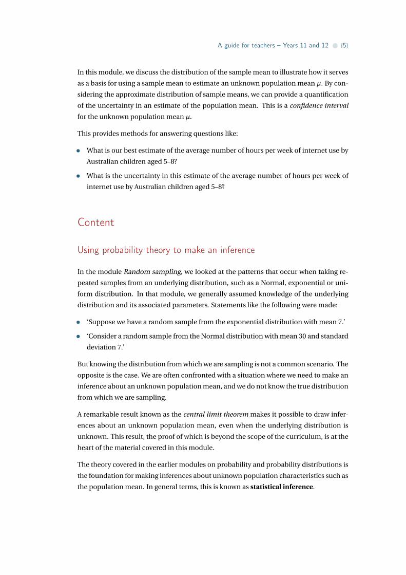
In this module, we discuss the distribution of the sample mean to illustrate how it serves

as a basis for using a sample mean to estimate an unknown population mean µ. By con-

sidering the approximate distribution of sample means, we can provide a quantification

of the uncertainty in an estimate of the population mean. This is a confidence interval

for the unknown population mean µ.

This provides methods for answering questions like:

• What is our best estimate of the average number of hours per week of internet use by

Australian children aged 5–8?

• What is the uncertainty in this estimate of the average number of hours per week of

internet use by Australian children aged 5–8?

Content

Using probability theory to make an inference

In the module Random sampling, we looked at the patterns that occur when taking re-

peated samples from an underlying distribution, such as a Normal, exponential or uni-

form distribution. In that module, we generally assumed knowledge of the underlying

distribution and its associated parameters. Statements like the following were made:

• ‘Suppose we have a random sample from the exponential distribution with mean 7.’

• ‘Consider a random sample from the Normal distribution with mean 30 and standard

deviation 7.’

But knowing the distribution from which we are sampling is not a common scenario. The

opposite is the case. We are often confronted with a situation where we need to make an

inference about an unknown population mean, and we do not know the true distribution

from which we are sampling.

A remarkable result known as the central limit theorem makes it possible to draw infer-

ences about an unknown population mean, even when the underlying distribution is

unknown. This result, the proof of which is beyond the scope of the curriculum, is at the

heart of the material covered in this module.

The theory covered in the earlier modules on probability and probability distributions is

the foundation for making inferences about unknown population characteristics such as

the population mean. In general terms, this is known as statistical inference.

{6} • Inference for means

The sample mean X as a point estimate of µ

Even without using any ideas from probability or distribution theory, it seems com-

pelling that the sample mean should tell us something about the population mean. If

we have a random sample from the population, the sample should be representative of

the population. So we should be able to use the sample mean as an estimate of the pop-

ulation mean.

We first review the definition of a random sample; this material is also covered in the

module Random sampling.

Consider a random variable X . The population mean µ is the expected value of X , that

is, µ= E(X ). In general, the distribution of X and the population mean µ are unknown.

A random sample ‘on X ’ of size n is defined to be n random variables X1, X2, . . . , Xn that

are mutually independent and have the same distribution as X .

We may think of the distribution of X as the underlying or ‘parent’ distribution, produc-

ing n ‘offspring’ that make up the random sample. We use the phrase ‘parent distribution’

throughout this module to refer to the underlying distribution from which the random

samples come.

There are some important features of a random sample defined in this way:

• Any single element of the random sample, Xi , comes from the parent distribution,

defined by the distribution of X . The distribution of Xi is the same as the distribution

of X . So the chance that Xi takes any particular value is determined by the shape and

pattern of the distribution of X .

• There is variation between different random samples of size n from the same under-

lying population distribution. Appreciating the existence of this variation and under-

standing it is central to the process of statistical inference.

• If we take a very large random sample from X , and draw a histogram of the sample,

the shape of the histogram will tend to resemble the shape of the distribution of X .

• If n is small, the evidence from the sample about the shape of the parent distribu-

tion will be very imprecise: the sample may be consistent with a number of different

parent distributions.

• Independence between the Xi ’s is a crucial feature: if the Xi ’s are not independent,

then the features we discuss here may not apply, and often will not apply.


We define the sample mean X of the random sample X1, X2, . . . , Xn as

X =∑n

i=1 Xi

n.

Once we obtain an actual random sample x1, x2, . . . , xn from the random variable X , we

have an actual observation

x =∑n

i=1 xi

n

of the sample mean. We call the observed value x a point estimate of the population

mean µ.

This discussion is reminding us that the sample mean X is actually a random variable; it

would vary from one sample to the next.

As there is a distinction to be made between the random variable X and its correspond-

ing observed value x, we refer to the random variable as the estimator X , and the ob-

served value as the estimate x; note the use of upper and lower case. Since both of these

may be referred to as the ‘sample mean’, we need to be careful about which of the two is

meant, in a given context.

This is exactly parallel to the situation in the module Inference for proportions, in which

the ‘sample proportion’ may refer to the estimator P , which is a random variable, or to

an observed value of this random variable, the estimate p.

In summary: The sample mean X is a random variable.

We now explore this important fact in some detail.

The sample mean as a random variable

In the module Random sampling, we examined the variability of samples of a fixed size n

from a variety of continuous population distributions. We saw, for example, a number of

random samples of size n = 10 from a Normal population with meanµ= 30 and standard

deviation σ= 7. The population modelled by this distribution is the population of study

scores of Year 12 students in a given subject.

Figure 1 is the first set of ten randomly sampled study scores from N(30,72) shown in

the module Random sampling. The sample has been projected down to the x-axis in the

lower part of figure 1 to give a dotplot of the data, and now the sample mean is shown as

a black triangle under the dots.


1

5144373023169

5144373023169Study score

from a Normal distribution of study scores, with mean=30, standard deviation=7

Ten randomly sampled study scores

Mean of the sample of ten study scores

Figure 1: First random sample of size n = 10 from N(30,72), with the sample mean shownas a triangle.

Figure 2 shows another random sample of size 10 from the same parent Normal distri-

bution N(30,72). The lower part of figure 2 shows both the first and second samples and

their means. We see that repeated samples from the same distribution have different

means — this is something we would expect, given that the observations in the repeated

samples from the same distribution are different from each other. It is the variation in

sample means that we focus on in this module.

1

5144373023169



Another ten randomly sampled study scores

Mean of the first sample of ten study scores

Mean of the second sample of ten study scores

Figure 2: Second random sample of size n = 10 from N(30,72).


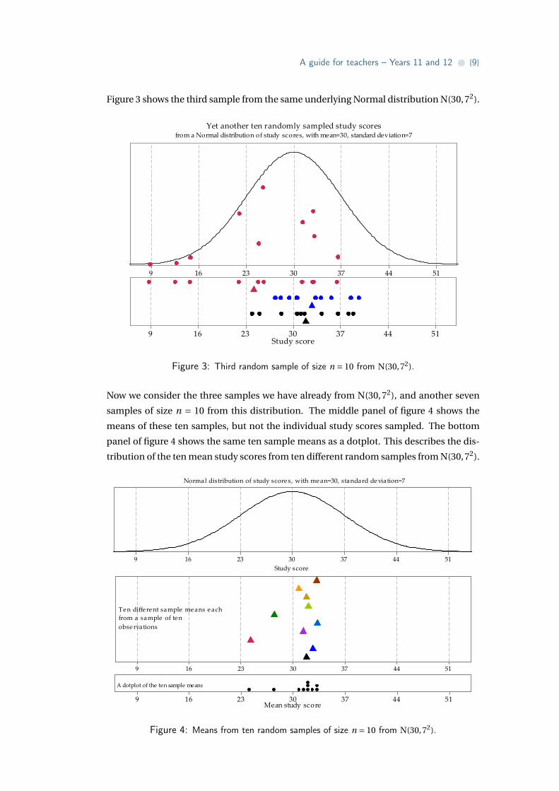
Figure 3 shows the third sample from the same underlying Normal distribution N(30,72).

1

5144373023169



Yet another ten randomly sampled study scores

Figure 3: Third random sample of size n = 10 from N(30,72).

Now we consider the three samples we have already from N(30,72), and another seven

samples of size n = 10 from this distribution. The middle panel of figure 4 shows the

means of these ten samples, but not the individual study scores sampled. The bottom

panel of figure 4 shows the same ten sample means as a dotplot. This describes the dis-

tribution of the ten mean study scores from ten different random samples from N(30,72).

1

5144373023169

Study score

5144373023169

5144373023169Mean study score

Normal distribution of study scores, with mean=30, standard deviation=7

observations

from a sample of ten

Ten different sample means each

A dotplot of the ten sample means

Figure 4: Means from ten random samples of size n = 10 from N(30,72).


We extend this idea in figure 5, which shows a histogram of the means of 100 samples of

size 10 from the Normal distribution N(30,72). The choice of 100 as the number to show

is arbitrary; all that is intended is to show a large enough number of sample means to

provide an idea of how much variation there can be among such sample means. Figure 5

shows the population distribution from which the samples are taken in the top panel,

and the histogram of sample means in the bottom panel.

1

5144373023169

Study score

5144373023169

20

15

10

5

0

Mean study score

Frequency

Normal distribution of study scores, with mean=30, standard deviation=7

(Each mean is based on a random sample of 10 observations)

Figure 5: Histogram of means from 100 random samples of size n = 10 from N(30,72).

There are a number of features to note in figure 5. The sample means are roughly centred

around 30. They range in value from about 24 to 35. There is variability in the sample

means, but it is smaller than the variability in the population from which the samples

were taken. The third sample mean, shown in red in figure 3, appears to be quite dif-

ferent from the first and second sample means; it is represented in the lowest bar of the

histogram in figure 5.

In summary: The sample mean X is a random variable, with its own distribution.

The mean and variance of X

We have seen that sample means can vary from sample to sample, and hence that the

sample mean X has a distribution. The way to think about this distribution is to imagine

an endless sequence of samples taken from a single population under identical condi-

tions. From this imagined sequence, we could work out each sample mean, and then


look at the distribution of them. This thought experiment helps us to understand what is

meant by ‘the distribution of X ’. We have approximated this thought experiment in the

previous section (figure 5), using only 100 samples. This is a long way short of an endless

sequence, but illustrates the idea.

What is the mean of this distribution? And its variance?

The visual impression we get from the example of 100 samples of study scores in the

previous section (figure 5) is that the mean of the distribution of the sample mean X is

equal to 30. So the distribution of X is centred around the mean of the underlying parent

distribution, µ. We will prove that this is true in general.

Since X comes from a random sample on X , it is hardly surprising that the properties of

the distribution of X are related to the distribution of X .

To obtain the mean and variance of X , we use two results covered in the module Binomial

distribution, which we restate here:

1 For n random variables X1, X2, . . . , Xn , we have

E(X1 +X2 +·· ·+Xn) = E(X1)+E(X2)+·· ·+E(Xn).

2 If Y1,Y2, . . . ,Yn are independent random variables, then

var(Y1 +Y2 +·· ·+Yn) = var(Y1)+var(Y2)+·· ·+var(Yn).

Theorem (Mean of the sample mean)

For a random sample of size n on X , where E(X ) =µ, we have

E(X ) =µ.

ProofEach random variable Xi in the random sample has the same distribution as X ,

and so E(Xi ) =µ. Also, recall that if Y = aV +b, then E(Y ) = a E(V )+b. Hence,

E(X ) = E( X1 +X2 +·· ·+Xn

n

)

= 1

nE(X1 +X2 +·· ·+Xn)

= 1

n

(µ+µ+·· ·+µ)

= 1

nnµ

=µ.


This is an important result. It tells us that, on average, the sample mean is neither too low

nor too high; its expected value is the population mean µ. The mean of the distribution

of the sample mean is µ. We may feel that this result is intuitively compelling or, at least,

unsurprising. But it is important nonetheless. It tells us that using the sample mean to

estimate µ has the virtue of being an unbiased method: on average, we will be right.

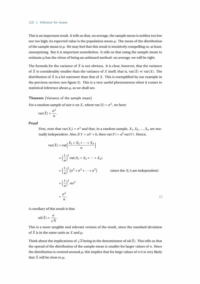
The formula for the variance of X is not obvious. It is clear, however, that the variance

of X is considerably smaller than the variance of X itself; that is, var(X ) ¿ var(X ). The

distribution of X is a lot narrower than that of X . This is exemplified by our example in

the previous section (see figure 5). This is a very useful phenomenon when it comes to

statistical inference about µ, as we shall see.

Theorem (Variance of the sample mean)

For a random sample of size n on X , where var(X ) =σ2, we have

var(X ) = σ2

n.

ProofFirst, note that var(Xi ) = σ2 and that, in a random sample, X1, X2, . . . , Xn are mu-

tually independent. Also, if Y = aV +b, then var(Y ) = a2 var(V ). Hence,

var(X ) = var( X1 +X2 +·· ·+Xn

n

)

=( 1

n

)2var(X1 +X2 +·· ·+Xn)

=( 1

n

)2 (σ2 +σ2 +·· ·+σ2) (since the Xi ’s are independent)

=( 1

n

)2nσ2

= σ2

n.

A corollary of this result is that

sd(X ) = σpn

.

This is a more tangible and relevant version of the result, since the standard deviation

of X is in the same units as X and µ.

Think about the implications ofp

n being in the denominator of sd(X ). This tells us that

the spread of the distribution of the sample mean is smaller for larger values of n. Since

the distribution is centred around µ, this implies that for large values of n it is very likely

that X will be close to µ.


Example

Consider the study-score example illustrated in the previous section, in which random

samples of size n = 10 are obtained from N(30,72). In this case:

• E(X ) = 30

• var(X ) = 4910 = 4.9

• sd(X ) =p4.9 = 2.21.

It is important to understand that these results for the mean, variance and standard de-

viation of X do not require the distribution of X to have any particular form or shape; all

that is required is for the parent distribution to have a meanµ and a varianceσ2. Further,

the results are true for all values of the sample size n.

In summary, for a random sample of n observations on a random variable X with meanµ

and variance σ2:

• E(X ) =µ

• var(X ) = σ2

n

• sd(X ) = σpn

.

Sampling from symmetric distributions

We found the mean and variance of the sample mean X in the previous section. What

more can be said about the distribution of X ? We now consider the shape of the distri-

bution of the sample mean.

It is instructive to consider random samples from a variety of parent distributions.

Sampling from the Normal distribution

When exploring the concept of a sample mean as a random variable, we used the ex-

ample of sampling from a Normal random variable. Specifically, we considered taking a

random sample of size n = 10 from the N(30,72) distribution. Figure 5 illustrated an ap-

proximation to the distribution of X in this case, by showing a histogram of 100 sample

means from random samples of size n = 10.

To approximate the distribution better, we take a lot more samples than 100. Figure 6

shows a histogram of 100 000 sample means based on 100 000 random samples each of

size n = 10. Each of the random samples is taken from the Normal distribution N(30,72).


1

5144373023169

4000

3000

2000

1000

0

Mean study score

Frequency

Histogram of 100,000 means

Normal distribution with mean = 30 and standard deviation = 7

Each mean is based on ten study scores randomly sampled from a

Figure 6: Histogram of means from 100 000 random samples of size n = 10 from N(30,72).

Although 100 000 is a lot of samples, it is still not quite an ‘endless’ repetition! If we took

more and more samples of size 10, each time obtaining the sample mean and adding it to

the histogram, then the shape of the histogram would become smoother and smoother

and more and more bell-shaped, until eventually it would become indistinguishable

from the shape of the Normal curve shown in figure 7.

Figure 7 shows the true distribution of sample means for samples of size n = 10 from

N(30,72), which is only approximated in figures 5 and 6.1

5144373023169

Mean study score

Normal distribution with mean = 30 and standard deviation = 7

Each mean is based on ten study scores randomly sampled from a

Distribution of sample means

Figure 7: The distribution of the sample mean X based on random samples of size n = 10

from N(30,72), with Xd= N(30, 72

10 ).


If we are sampling from a Normal distribution, then the distribution of X is also Normal,

a result which we assert without proof. This result is true for all values of n.

Theorem (Sampling from a Normal distribution)

If we have a random sample of size n from the Normal distribution with mean µ and

variance σ2, then the distribution of the sample mean X is Normal, with mean µ and

variance σ2

n . In other words, for a random sample of size n on Xd= N(µ,σ2), the distribu-

tion of the sample mean is itself Normal: specifically, Xd= N(µ, σ

2

n ).

We have observed that the spread of the distribution of X is less than that of the distri-

bution of the parent variable X . This reflects the intuitive idea that we get more precise

estimates from averages than from a single observation. Further, since the sample size n

is in the denominator of the variance of X , the spread of sample means in a long-run

sequence based on samples of size n = 1000 each time (for example) will be smaller than

the spread of sample means in a long-run sequence based on samples of size n = 50.

Again consider taking repeated samples of study scores from the Normal distribution

N(30,72). Four different scenarios are shown in figure 8, each based on different sample

sizes of study scores: n = 1, n = 4, n = 9 and n = 25. In the top panel are histograms

based on 100 000 sample means, and in the bottom panel are the true distributions of

the sample means. The distributions of sample means based on larger sample sizes are

narrower, and more concentrated around the mean µ, than those based on smaller sam-

ples. The distribution of sample means based on one study score is, of course, identical

to the original population distribution of study scores.

1

5144373023169

15000

10000

5000

0

5144373023169 5144373023169 5144373023169

1 study score

Mean study score

Frequency4 study scores 9 study scores 25 study scores

5144373023169 5144373023169 5144373023169 5144373023169

1 study score

Mean study score

4 study scores 9 study scores 25 study scores

Each mean is based on a random sample (from a Normal distribution with mean = 30, standard deviation = 7) of:

Histograms of sample means

Distributions of sample means

Sample means for random samples (from a Normal distribution with mean = 30, standard deviation = 7) of:

Figure 8: Histograms and true distributions of means of random samples of varying sizefrom N(30,72).


Exercise 1

a Estimate the standard deviation of each of the distributions in the bottom panel of

figure 8.

b Calculate the standard deviation of each of the distributions in the bottom panel of

figure 8, and compare your estimates with the calculated values.

In summary: For a random sample of size n on Xd= N(µ,σ2), the distribution of X is itself

Normal; specifically,

Xd= N(µ, σ

2

n ).

It is very important to understand that sampling from a Normal distribution is a special

case. It is not true, for other parent distributions, that the distribution of X is Normal for

any value of n.

We now consider the distribution of sample means based on populations that do not

have Normal distributions.

Sampling from the uniform distribution

Recall that the uniform distribution is one of the continuous distributions, with the cor-

responding random variable equally likely to take any value within the possible interval.

If Xd= U(0,1), then X is equally likely to take any value between 0 and 1.

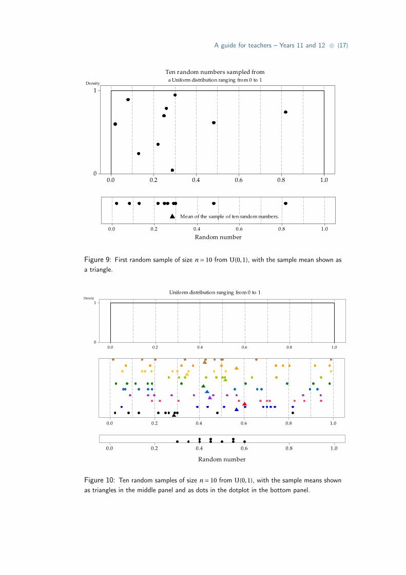
Figure 9 shows the first of several random samples of size n = 10 from the uniform distri-

bution U(0,1), as seen in the module Random sampling. The sample has been projected

down to the x-axis in the lower part of figure 9 to give a dotplot of the data, and now

the sample mean is added as a black triangle under the dots. The data in this case are

referred to as ‘random numbers’, since a common application of the U(0,1) distribution

is to generate random numbers between 0 and 1.

Figure 10 shows ten samples, each of 10 observations from the same uniform distribution

U(0,1). The top panel shows the population distribution. The middle panel shows each

of the ten samples, with dots for the observations and a triangle for the sample mean.

The bottom panel shows the ten sample means plotted on a dotplot.


1.00.80.60.40.20.0

1

0

Density

1.00.80.60.40.20.0

Random number

Ten random numbers sampled from

a Uniform distribution ranging from 0 to 1

Mean of the sample of ten random numbers.

Figure 9: First random sample of size n = 10 from U(0,1), with the sample mean shown asa triangle.

1

1.00.80.60.40.20.0

1

0

Density

1.00.80.60.40.20.0

1.00.80.60.40.20.0

Random number

Uniform distribution ranging from 0 to 1

Figure 10: Ten random samples of size n = 10 from U(0,1), with the sample means shownas triangles in the middle panel and as dots in the dotplot in the bottom panel.


Figure 11 shows a histogram with one million sample means from the same population

distribution. There are several features to note in figure 11. As in the case of the distri-

bution of sample means taken from a Normal population, the spread in the histogram of

sample means is less than the spread in the parent distribution from which the samples

are taken. However, in contrast to the case of sampling from a Normal distribution, the

shape of the histogram is unlike the population distribution; rather, it is like a Normal

distribution.

1

1.00.80.60.40.20.0

1

0

Random number

Density

1.00.80.60.40.20.0

10000

7500

5000

2500

0

Mean random number

Frequency

Uniform distribution ranging from 0 to 1

(Each mean is based on a random sample of ten observations)

Figure 11: Histogram of means from one million random samples of size n = 10 fromU(0,1).

Figure 12 shows four different histograms of means of samples of random numbers taken

from the uniform distribution U(0,1). From left to right, they are based on sample size

n = 1, n = 4, n = 16 and n = 25. Of course, when the sample mean is based on a single

random number (n = 1), the shape of the histogram looks like the original parent distri-

bution. The other histograms are not uniform; they tend to be bell-shaped. It is rather

remarkable that we see this is so even for a sample size as small as n = 4.


1

1.00.80.60.40.20.0

7000

6000

5000

4000

3000

2000

1000

01.00.80.60.40.20.0 1.00.80.60.40.20.0 1.00.80.60.40.20.0

1 random number

Mean random number

Frequency4 random numbers 16 random numbers 25 random numbers

Histograms of 100,000 means

Each mean is based on:

Figure 12: Histograms of means of random samples of varying size from U(0,1).

How does this tendency to a bell-shaped curve arise?

Consider the means of samples of size n = 4, for example. Figure 13 shows ten different

random samples taken from the uniform distribution U(0,1), each with four observa-

tions. The observations are shown as dots, and the means of the samples of four obser-

vations are shown as triangles. The darker vertical line at x = 0.5 shows the true mean for

the population from which the samples were taken.

Consider the values of the observations sampled in relation to the population mean. The

first sample in figure 13 has two values below 0.5, and two above; the mean of these four

values is close to 0.5. The second sample is similar, with two values below the true mean,

and two values above. Samples 3, 6 and 7 have three values below the mean, and only

one above. The means of these three samples are below the true mean, and they tend to

be further from 0.5 than samples 1 and 2. All four observations in sample 8 are above 0.5,

and all four observations in sample 10 are below 0.5; the means of these two samples are

farthest from the true population mean.

As the population from which the observations are sampled is uniform, samples with two

of the four observations above the mean of 0.5 will arise more often than samples with

one or three observations above 0.5; samples with zero or four observations above 0.5

will arise least often. Hence, we see the tendency for the histogram in the second panel

in figure 12 to be concentrated and centred around 0.5.


Statistical Consulting Centre 12 March 2013

Sample 10

Sample 9

Sample 8

Sample 7

Sample 6

Sample 5

Sample 4

Sample 3

Sample 2

Sample 1

1.00.80.60.40.20.0Random number

Figure 13: Ten random samples of size n = 4 from U(0,1), with the sample means shownas triangles.

Sampling from asymmetric distributions

We have examined the distribution of the sample mean when taking samples from Nor-

mal and uniform distributions. Both these types of population models are symmetric.

Now we consider taking samples from distributions that are not symmetric.

Sampling from the exponential distribution

An exponential distribution is ‘skewed’, with a much longer tail to the right-hand end

of the distribution than to the left. Again we use an example introduced in the module

Random sampling. In the example, it was assumed that the underlying random variable

represents the interval between births at a country hospital; the average time between

births is seven days. We assume that the distribution of the time between births follows

an exponential distribution. This means that the random variable X from which we are

sampling has an exponential distribution with rate 17 , that is, X

d= exp( 17 ).

Figure 14 shows the model for the time between births in the top panel, and the first of

several sets of ten random observations from the model in the bottom panel. The mean

for this particular set of ten observations is 6.9 days, shown as a black triangle under the


dotplot of the observations. Figure 15 shows ten different samples of ten observations,

with the sample means. The bottom panel in figure 15 provides a dotplot of the ten

sample means.

1

50403020100

1/7

0

Density

50403020100

Number of days between births

from an Exponential distribution with a mean = 7 days

Ten random observations

Mean of the first se t of ten random observations

Figure 14: First random sample of size n = 10 from exp( 17 ), with the sample mean shown

as a triangle.

1

50403020100

1/7

0


Density

50403020100

Mean number of days between births

Exponential distribution with a mean = 7 days

Ten different sample means (triangles)

each from a sample of ten random observations

Dotplot of the ten sample means

Figure 15: Ten random samples of size n = 10 from exp( 17 ), with the sample means shown

as triangles.


We have looked at just a few samples of size n = 10, and represented the sample means

obtained in a dotplot. What happens if we take many such samples, and graph the his-

togram of the sample means? Figure 16 shows the histogram of 100 sample means from

samples of size n = 10. The histogram is somewhat bell-shaped, much closer to being

symmetrical than the distribution of X , and narrower.

1

50403020100

1/7

0


Density

50403020100

20

15

10

5

0


Frequency



Figure 16: Histogram of means from 100 random samples of size n = 10 from exp( 17 ).

Even with 100 sample means, the distribution is not smooth. To make it smoother, in

figure 17 we show the histogram based on one million sample means from samples of

size n = 10.


1

50403020100

1/7

0


Density

50403020100

20000

15000

10000

5000

0


Frequency



Figure 17: Histogram of means from one million random samples of size n = 10 fromexp( 1

7 ).

Exercise 2

Consider a random sample of size n = 10 from exp( 17 ).

a Find the following quantities:

i E(X )

ii var(X )

iii sd(X ).

b Relate the mean E(X ) of X and the standard deviation sd(X ) of X to the histogram

shown in figure 17.

The sample means in figures 16 and 17 are based on samples with the small sample size

of n = 10. Figure 17 shows one million means, each based on 10 observations; the his-

togram of sample means is asymmetric, with a tail to the right.

Figure 18 shows the true distribution of sample means for samples of size n = 10 from

the exp( 17 ) distribution, the derivation of which is beyond the curriculum. This is the

true distribution corresponding to the histograms in figures 16 and 17.



20151050

0.20

0.15

0.10

0.05

0.00


Density

Distribution of sample means for random samples of n = 10 from an exponential distribution (mean = 7 days)

Figure 18: The true distribution of the sample mean X based on random samples of sizen = 10 from exp( 1

7 ).

What happens if we increase the sample size n? In figure 19, the means are based on

samples of size n = 50 and, in figure 20, the means are based on size n = 200. In both

cases, histograms of a large number of sample means are shown, to get a reliable idea

of the true shape. In comparison with figure 17, the histograms of the means are more

symmetric and even closer to bell-shaped.

1

1211109876543

2000

1500

1000

500

0


Frequency

Histogram of 100,000 sample means

Exponential distribution with mean = 7)

(Each mean is based on a random sample of 50 observations from an

Figure 19: Histogram of sample means from random samples of size n = 50 from exp( 17 ).


1

1098765

2000

1500

1000

500

0


Frequency

Histogram of 50,000 sample means

from an Exponential distribution with mean = 7)

(Each mean is based on a random sample of 200 observations

Figure 20: Histogram of sample means from random samples of size n = 200 from exp( 17 ).

Figure 21 illustrates why the histograms of means based on larger sample sizes tend to be

more symmetric than those based on smaller samples. The top panel shows a random

sample of five observations from the exponential distribution we are considering. There

is one relatively extreme observation of 37.6 days; the sample mean based on the five

observations, shown as a triangle, is 11.2 days. In a small sample, a single observation

in the long right-hand tail of the distribution will have a noticeable effect on the sample

mean: it will ‘drag it’ to the right.

423528211470


Sample of 30

Sample of 10

Sample of 5

(Sample mean shown as a triangle )

Figure 21: Dotplots of three samples from exp( 17 ), with sample means shown as triangles.


The darker vertical line in figure 21 shows the true population mean of 7 days. In the

second panel, five more observations are added to the sample; the sample mean for these

ten observations is 8.7. This is closer to 7, even though the sample still contains the

unusual observation, because the larger number of observations close the mean have a

lot of weight in the average.

With yet more observations, the extreme value has even less influence on the sample

mean. In the bottom panel, 20 more random observations have been added to the sam-

ple, giving 30 in total; the sample mean is 6.4, which is closer to the true population mean

than the means of the two smaller samples.

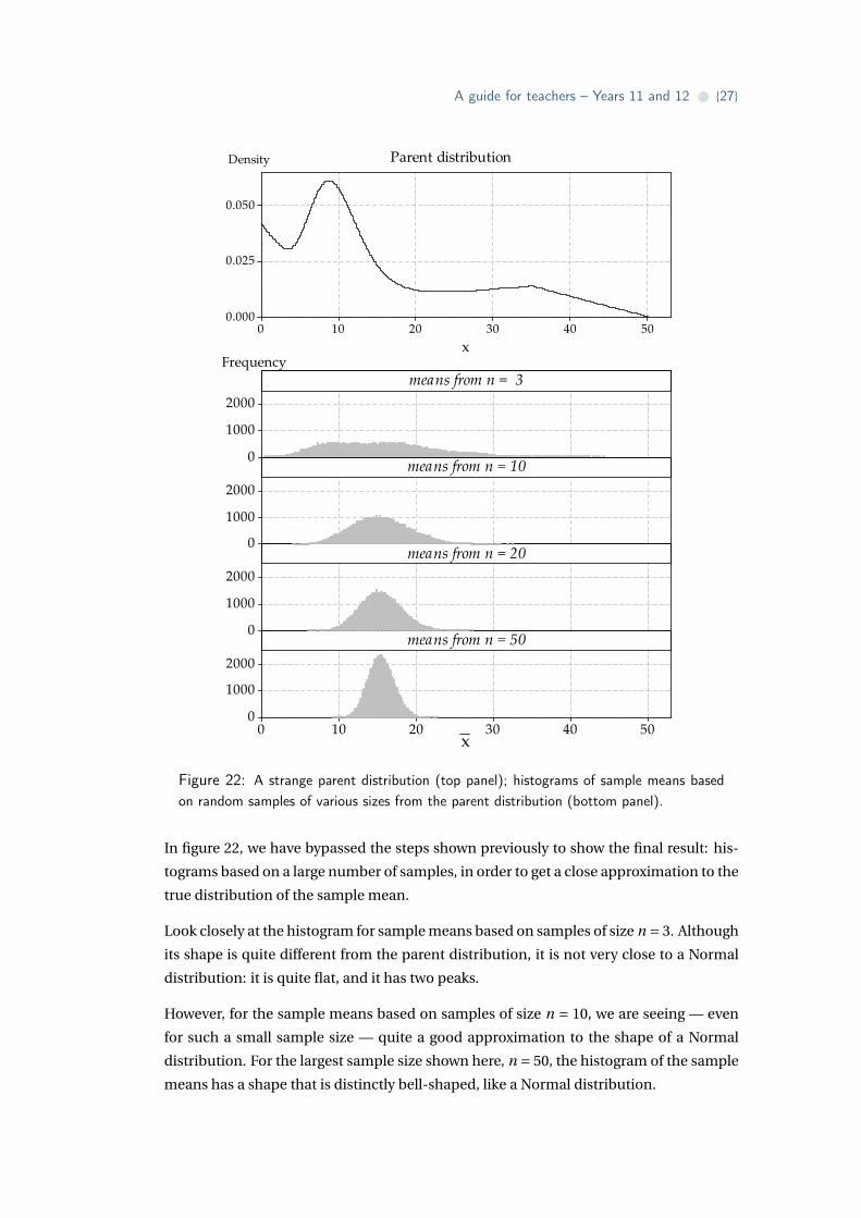
Sampling from a strange distribution

So far we have looked at sampling from known, named distributions: the Normal, uni-

form and exponential distributions. What happens if the distribution from which we are

sampling is strange? This is illustrated in figure 22, in which we sample from the weird-

looking distribution shown in the top panel.

Exercise 3

Consider the probability density function (pdf) shown in the top panel of figure 22.

a Use the graph of the pdf to check visually (to the extent possible) that the function in

the graph satisfies the properties of a pdf.

b One of the following values is the mean of the corresponding random variable. Which

is it?

i 10.1

ii 15.4

iii 19.0

iv 24.4

c One of the following values is the standard deviation of the corresponding random

variable. Which is it?

i 4

ii 8

iii 12

iv 16



50403020100

0.050

0.025

0.000

x

Density

2000

1000

0

2000

1000

0

2000

1000

0

50403020100

2000

1000

0

means from n = 3

x

Frequency

means from n = 10

means from n = 20

means from n = 50

Parent distribution

Figure 22: A strange parent distribution (top panel); histograms of sample means basedon random samples of various sizes from the parent distribution (bottom panel).

In figure 22, we have bypassed the steps shown previously to show the final result: his-

tograms based on a large number of samples, in order to get a close approximation to the

true distribution of the sample mean.

Look closely at the histogram for sample means based on samples of size n = 3. Although

its shape is quite different from the parent distribution, it is not very close to a Normal

distribution: it is quite flat, and it has two peaks.

However, for the sample means based on samples of size n = 10, we are seeing — even

for such a small sample size — quite a good approximation to the shape of a Normal

distribution. For the largest sample size shown here, n = 50, the histogram of the sample

means has a shape that is distinctly bell-shaped, like a Normal distribution.


The central limit theorem

We have already described two important properties of the distribution of the sample

mean X that are true for any value of the sample size n. These two properties are that

E(X ) =µ and var(X ) = σ2

n .

There is a third property of the distribution of the sample mean X that does depend on

the value of the sample size n. However, this remarkable property does not depend on the

shape of the distribution of X , the parent distribution from which the random sample is

taken. It is known as the central limit theorem and is stated as follows.

Theorem (Central limit theorem)

For large samples, the distribution of the sample mean is approximately Normal. If we

have a random sample of size n from a parent distribution with mean µ and variance σ2,

then as n grows large the distribution of the sample mean X tends to a Normal distribu-

tion with mean µ and variance σ2

n .

The extremely useful implication of this result is that, for large samples, the distribution

of the sample mean is approximately Normal.

This is a startling property because there are no restrictions on the shape of the popula-

tion distribution of X ; all we specify are its mean and variance. The population distribu-

tion might be a uniform distribution, an exponential distribution or some other shape: a

U-shape, a triangular shape, extremely skewed or quite irregular.

Note. For the central limit theorem to apply, we do need the parent distribution to have a

mean and variance! There are some strange distributions for which either the variance,

or the mean and the variance, do not exist. But we need not worry about such distribu-

tions here.

The central limit theorem has a long history and very wide application. It is beyond the

scope of the curriculum to provide a proof, but we have already seen empirical evidence

of its truth: examples showing the behaviour of the distribution of the sample mean as

the sample size n increases.

As the averages from any shape of distribution tend to have a Normal distribution, pro-

vided the sample size is large enough, we do not need information about the parent

distribution of the data to describe the properties of the distribution of sample means.

Therein lies the power of the central limit theorem, since limited knowledge about the

parent distribution is the norm. We have a basis for using the sample mean to make in-

ferences about the population mean, even in the usual situation where we don’t know

the distribution of X , the random variable we are sampling.


The central limit theorem is the result behind the phenomenon we have seen in the ex-

amples in the previous sections. Each time we looked at samples of a large size, the

histogram of the sample means was bell-shaped and symmetrically positioned around

the mean of the parent distribution.

This important result is used for inference about the unknown population mean µ; but

there is one more step in this process.

Standardising the sample mean

The module Exponential and normal distributions shows how any Normal distribution

can be standardised, in the following way, to give a standard Normal distribution:

If Yd= N(µ,σ2) and Z = Y −µ

σ, then Z

d= N(0,1).

The standard Normal distribution has mean 0 and variance 1. A random variable with

this distribution is usually denoted by Z . That is, Zd= N(0,1).

Consider a standardisation of X . We subtract off the mean of X , which is µ, and divide

through by the standard deviation of X , which is σpn

, to obtain a standardised version of

the sample mean:

X −µσ/

pn

.

Now we ask: What is the distribution of this quantity?

Sampling from a Normal distribution

We first consider the case of a random sample from a Normal population, say the popu-

lation of study scores N(30,72).

The standardisation of X for this example is illustrated in figure 23. There are nine distri-

butions in figure 23.

• The top row, moving from left to right, shows the distribution of the sample mean X

for random samples of size n = 30, n = 50 and n = 100.

• The middle row shows the distributions of X −µ; all the distributions are now centred

at 0, but the spread of the distributions still varies, and still depends on n.

• The bottom row shows the distributions ofX −µσ/

pn

; the three distributions of the stan-

dardised versions of X have the same centre and spread. The mean is 0 and the stan-

dard deviation is 1.


Of course, all nine distributions in figure 23 are Normal distributions. As we saw in a pre-

vious section (Sampling from symmetric distributions), if the parent distribution from

which we are sampling is Normal, then the distribution of the sample mean is itself Nor-

mal, for any n.

353025 353025 353025

50‐5 50‐5 50‐5

20‐2 20‐2 20‐2

n = 30 n = 50 n = 100

/√

/√

/√

Figure 23: Standardisation of the distribution of X for samples from a Normal distribution,for various values of n.

In summary: For a random sample of size n from a Normal distribution,

X −µσ/

pn

d= N(0,1).

Under the specific conditions of sampling from a Normal distribution (and only then),

this result holds for any value of n.

Sampling from the uniform distribution

Now consider the distribution of the sample mean for random samples from the uniform

distribution U(0,1). We illustrate this in figure 24 with simulations of 100 000 samples.

• The top row, moving from left to right, shows the histogram of the sample mean X for

random samples of size n = 30, n = 50 and n = 100. The histograms in the top row are

symmetric and bell-shaped; there is greater variability when the means are based on

smaller sample sizes.


• The middle row shows the histograms of X −µ; all are now centred at 0, but the spread

of the distributions still depends on n, in the same way as it does in the top row.

• The bottom row shows the histograms ofX −µσ/

pn

. Now all of the histograms look very

similar; they have the same centre and spread. The mean is 0 and the standard de-

viation is 1, and they are bell-shaped; in short, they have approximately the same

distribution as Zd= N(0,1).

0.70.60.50.40.3

3000

1500

0

0.70.60.50.40.3 0.70.60.50.40.3

Frequency

0.20.10.0‐0.1‐0.2

3000

1500

0

0.20.10.0‐0.1‐0.2 0.20.10.0‐0.1‐0.2

3210‐1‐2‐3

3000

1500

0

3210‐1‐2‐3 3210‐1‐2‐3

n = 30 n = 50 n = 100

/√

/√

/√

Figure 24: Standardisation of the distribution of X for samples from a uniform distribution,for various values of n.

This shows via simulation the application of the central limit theorem to the uniform

distribution: for a random sample of size n from the uniform distribution, if n is large,

then

X −µσ/

pn

d≈ N(0,1).

Sampling from the exponential distribution

Next we consider standardisation of the distribution of sample means for samples from

the exponential distribution with mean 7; see figure 25. This figure is based on the true

distribution of the sample mean, as in this case it can be derived explicitly. (So we do

not need to rely on histograms of sample means from many random samples to get an

approximate idea of the distributions involved.)



8.57.05.5 8.57.05.5 8.57.05.5

1.50.0‐1.5 1.50.0‐1.5 1.50.0‐1.5

20‐2 20‐2 20‐2

n = 100 n = 200 n = 400

/√

/√

/√

Figure 25: Standardisation of the distribution of X for samples from the exponentialdistribution exp( 1

7 ), for various values of n.

We have already seen the distribution of the sample mean X based on random samples

of size n = 10 from exp( 17 ), in the section Sampling from asymmetric distributions (see

figure 18). For the case n = 10, the value of n is small and, although the distribution of X

is much more symmetric that the distribution of X itself, some skewness is still apparent.

Now, in figure 25, we look at considerably larger sample sizes.

• The top row of figure 25, moving from left to right, shows the distribution of the sam-

ple mean X for random samples from exp( 17 ) for n = 100, n = 200 and n = 400.

• The middle row shows the distributions of X −µ; all the distributions are centred at 0,

but the spread of the distributions still depends on n.

• The bottom row shows the distributions ofX −µσ/

pn

; now all the distributions have the

same centre and spread. The mean is 0 and the standard deviation is 1.

For these larger values of n, can you still detect some skewness visually? Are these dis-

tributions symmetric? There is some slight skewness apparent . . . but you have to look

hard! The distribution is approximately Normal, and the approximation is quite good for

these large values of n.

Keep in mind how good this approximation is for these values of n, given the substantial

skewness of the parent exponential distribution.


This shows the application of the central limit theorem to the exponential distribution:

for a random sample of size n from the exponential distribution, if n is large, then

X −µσ/

pn

d≈ N(0,1).

We have shown examples for the uniform and exponential distributions, but the condi-

tions of the central limit theorem are completely general: it works for any distribution

with a finite mean µ and finite variance σ2.

The Normal approximation described here is used later, when we obtain an approximate

confidence interval for the unknown population mean µ, based on a random sample.

Before getting to the practicalities, however, we consider some very important general

ideas about confidence intervals.

Population parameters and sample estimates

The mean study score for the population of all Year 12 students taking a particular sub-

ject is an example of a population parameter. It is important to make the distinction

between this population parameter and a sample estimate. In practice, we are interested

in finding out about an unknown population parameter, the mean µ. This has a fixed but

unknown value: it is a number. We collect data from a random sample in order to ob-

tain a sample estimate of this population parameter. As we have illustrated repeatedly,

it is most unlikely that different samples from the same population will give the same

estimate: rather, they will vary.

The unknown population parameter, the true mean, is µ. An estimate we obtain from

a single sample, the sample mean, is the point estimate x. The aim of the methods we

describe later in this module is to infer something about the parameter of a population

from the sample. This is an inference because there is uncertainty about the parameter.

We can however, quantify this uncertainty, and the theory we have been looking at, based

on the distribution of sample means, is what is required for this task.

Confidence intervals

This section deals with fundamental aspects of confidence intervals. In the next section,

we will deal with obtaining a confidence interval for the specific case we are considering,

but it is important first to understand confidence intervals conceptually.

A sample mean x is a single point or value that provides us with an estimate of the true

mean of interest in the population. In some sense, we are not interested in the partic-

ular value of the sample mean per se, but rather we are interested in the information it


provides us about the population. It provides an estimate of the population parameter

of interest; in this case, the mean in the population, µ.

While the mean from the sample will provide us with the best estimate of the population

mean, it is unlikely that the sample value will be exactly equal to the parameter being

estimated. Hence, the sample estimate is most useful if it is combined with some infor-

mation about its precision.

Suppose, for example, we want to estimate the mean µ of study scores for a particular

Year 12 subject, and that we have two different random samples of study scores for this

subject available. The first sample provides an estimate of the true mean of 29.1, while

the second sample provides the estimate 27.5. These estimates may seem inconsistent,

and it may be unclear which we might prefer to rely on. However, if the first sample mean

is likely to be within ±1.4 of the true value of µ, and the second sample mean is likely to

be within ±5.0 of the true value of µ, then the first result is more precise than the second.

By describing the first result as 29.1±1.4, we are specifying an interval or range of values

(from 29.1−1.4 to 29.1+1.4) within which we have confidence that the true value of µ

lies. The interval has a lower bound and an upper bound: 27.7 and 30.5, respectively.

This interval is an indicator of the precision of the estimate of the population mean and

is called a confidence interval. ‘Confidence’ has a particular meaning in this context,

which we now describe.

Confidence level

In working out a confidence interval, we decide on a ‘degree’ or ‘level’ of confidence.

This is quantified by the confidence level. In most applications, the confidence level

used is 95%.

The confidence level specifies the long-run percentage or proportion of confidence in-

tervals containing the true value — in this context, µ. Illustrating this idea requires a

simulation or a thought experiment. In practice, we typically have a single sample of

n observations, and we calculate x and a single confidence interval to characterise the

precision in the result. Any actual interval either contains or does not contain the true

value of the parameter µ. We don’t know, for example, if the interval 27.7 to 30.5 for the

mean study score contains the true value. The confidence level — 95% in this example

— does not mean that the chance of this particular interval containing µ is 0.95.

To illustrate the meaning of the confidence level, assume we know that the value of the

true mean study score µ is 30. The first random sample described above was based on

100 students and the mean was 29.1. We can imagine repeating this process many times,

sampling different students each time, and each time we will observe a different sample

mean.


Figure 26 shows the estimates and 95% confidence intervals from 100 such random sam-

ples, with the first result closest to the x-axis. For each random sample, the estimate of

the mean of interest is plotted as a dot in the centre of a line. The line shows the 95% con-

fidence interval for the particular random sample. For the first random sample, the line

showing the 95% confidence interval is from 27.7 to 30.5.

1

33323130292827

Mean study score with 95% confidence interval

Figure 26: 95% confidence intervals for the mean study score from 100 random samples,each of 100 students.


The darker vertical line in figure 26 corresponds to the true value of µ = 30. Most of the

confidence intervals are colored blue, but a small number are red; these are the confi-

dence intervals that do not include the true value of 30. In total, four of the 100 intervals

are red. In this small simulation, 96% of the intervals include the true value. We expect

that, on average, 95% of the 95% confidence intervals will include the true value, and this

is the real meaning of the ‘95%’; with much larger simulations, the percentage would be

very close to 95%.

Varying the confidence level

Figure 27 shows the same 100 random samples of 100 students again. For each random

sample, the estimate of the mean of interest is plotted as a dot in the centre of a line

which this time shows the 50% confidence interval. Because they represent the same

samples, the dots in figure 27 are at the same positions as those in figure 26.

Red lines correspond to confidence intervals that do not include the true value of the

parameter µ = 30. The 50% confidence intervals look narrow and precise, but figure 27

indicates that this is at a price. The intervals are narrower than the 95% confidence inter-

vals in figure 26, but around half of them do not include the true value of the parameter.

A guide for teachers – Years 11 and 12 • {37}1

3231302928

Mean study score with 50% confidence interval

Figure 27: 50% confidence intervals for the mean study score from 100 random samples,each of 100 students.


Consider figure 28, which shows confidence intervals for the mean study score from the

first random sample described above. The confidence intervals have different confi-

dence levels. When the confidence level is larger, the confidence interval is wider. This

is a natural consequence of the higher probability of including the true parameter value,

in the imagined long-run sequence of repetitions.

1

3130292827

Confidence intervals for the mean study score

50% confidence interval





Figure 28: Estimate of the mean study score from one random sample, with confidenceintervals using different confidence levels.

Exercise 4

Look at figure 28 and determine, without calculation,

a a 0% confidence interval for µ

b a 100% confidence interval for µ.

Calculating confidence intervals

Calculating a 95% confidence interval with the Normal approximation

We have seen that the sample mean X has mean µ and variance σ2

n , and that the dis-

tribution of X is approximately Normal when the sample size n is large. This raises the

question: How large is ‘a large sample size’? Appropriate guidelines need to take into ac-

count the nature of the population being sampled, as far as this is possible; this will be

elaborated later in this section.

The Normal approximation for the distribution of X tells us that, for large n,

X −µσ/

pn

d≈ N(0,1).


For a random variable with the standard Normal distribution, Zd= N(0,1), we know that

Pr(−2 < Z < 2) ≈ 0.95. To be more precise:

Pr(−1.96 < Z < 1.96) = 0.95.

We studied how to obtain the value 1.96 in the module Exponential and normal distribu-

tions. Figure 29 is a visual reminder.

Figure 29: The standard Normal distribution, Zd= N(0,1).

If we consider the Normal approximation to the distribution of the standardised sample

mean, it follows that we can state that, for large n,

Pr(−1.96 < X −µ

σ/p

n< 1.96

)≈ 0.95.

We multiply through by σpn

to obtain

Pr(−1.96

σpn< X −µ< 1.96

σpn

)≈ 0.95.

In other words, the distance between X and µ will be less than 1.96 σpn

for 95% of sample

means.

One further rearrangement gives

Pr(

X −1.96σpn<µ< X +1.96

σpn

)≈ 0.95.

It is really important to reflect on this probability statement. Note that it has µ in the

centre of the inequalities. The population parameter µ does not vary: it is fixed, but

unknown. The random element in this probability statement is the random interval

around µ.


This forms the basis for the approximate 95% confidence interval for the true mean µ.

In a given case, we have just a single sample mean x. An approximate 95% confidence

interval for µ is given by

x ±1.96σpn

.

However, a problem remains. The uncertainty in the estimate depends on σ, which is an

unknown parameter: the true standard deviation of the parent distribution.

In the approximate methods used here, we replace the population standard deviation σ

with the sample standard deviation.

The sample standard deviation is an estimate of the population standard deviation. Just

as X is a random variable that estimatesµ and has an observed value x for a specific sam-

ple, so S is a random variable that estimates σ and has an observed value s for a specific

sample. The sample standard deviation (which is dealt with in the national curriculum

in Year 10) is defined as follows. For a random sample X1, X2, . . . , Xn from a population

with standard deviation σ, the sample standard deviation is defined to be

S =√∑n

i=1(Xi − X )2

n −1,

where X is the sample mean. For a specific random sample x1, x2, . . . , xn , the observed

value of the sample standard deviation is

s =√∑n

i=1(xi − x)2

n −1,

where x is the observed value of the sample mean.

It is reasonable to ask whether using S in place of σ actually works. We have extensively

demonstrated the approximate Normality of the distribution of the sample mean. In

particular, we have seen that, for large n,

X −µσ/

pn

d≈ N(0,1).

But now it seems that we are going to rely on a different, further approximation, that for

large n,

X −µS/

pn

d≈ N(0,1).

The result that uses S in place ofσ is also valid; as n tends to infinity, the sample standard

deviation S gets closer and closer to the true standard deviation σ. We could revisit all

of the previous examples and demonstrate this for the uniform, exponential and so on;

instead, we use the strange-looking distribution to make the point.


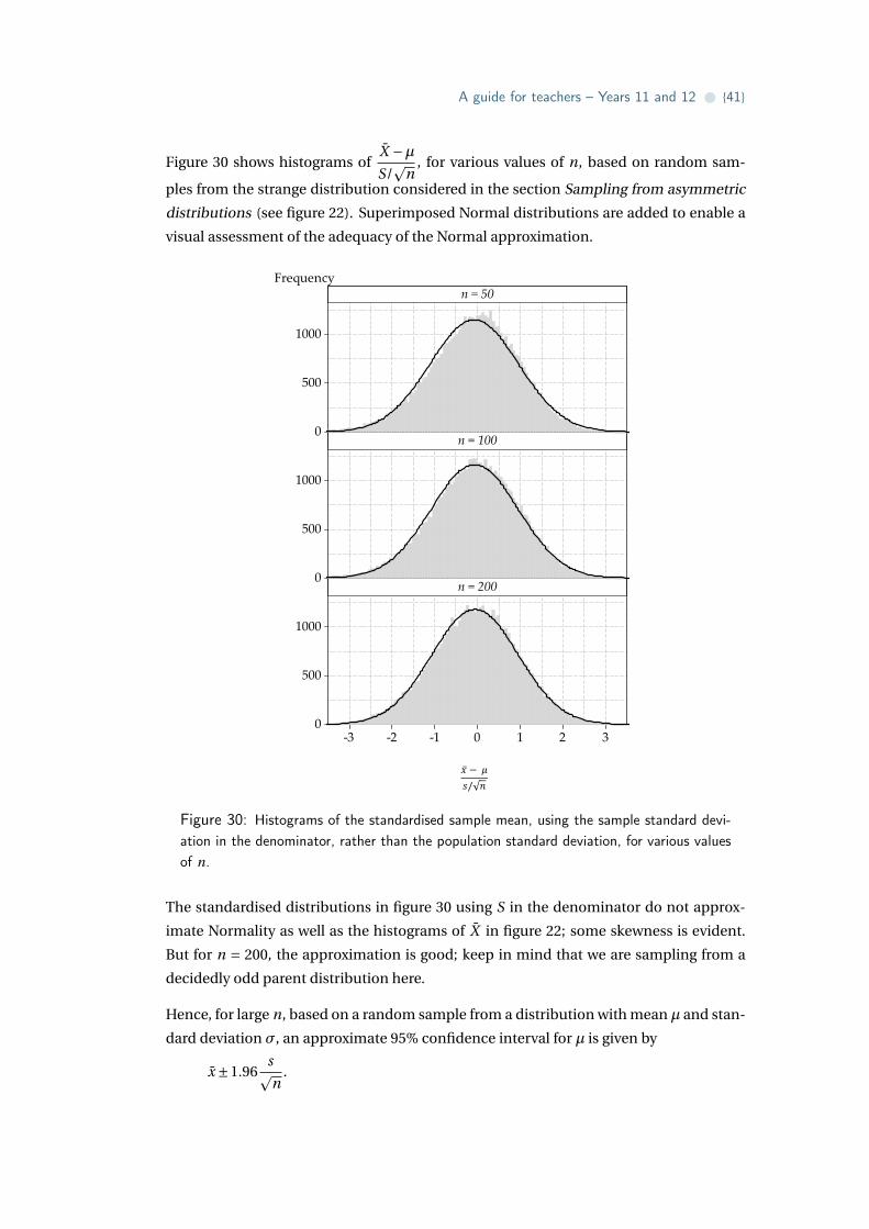
Figure 30 shows histograms ofX −µS/

pn

, for various values of n, based on random sam-

ples from the strange distribution considered in the section Sampling from asymmetric

distributions (see figure 22). Superimposed Normal distributions are added to enable a

visual assessment of the adequacy of the Normal approximation.


/√

1000

500

0

1000

500

0

3210‐1‐2‐3

1000

500

0

n = 50Frequency

n = 100

n = 200

Figure 30: Histograms of the standardised sample mean, using the sample standard devi-ation in the denominator, rather than the population standard deviation, for various valuesof n.

The standardised distributions in figure 30 using S in the denominator do not approx-

imate Normality as well as the histograms of X in figure 22; some skewness is evident.

But for n = 200, the approximation is good; keep in mind that we are sampling from a

decidedly odd parent distribution here.

Hence, for large n, based on a random sample from a distribution with mean µ and stan-

dard deviation σ, an approximate 95% confidence interval for µ is given by

x ±1.96spn

.


Example: Internet use by children

A recent large survey of a random sample of Australian children asked about weekly

hours of internet use in three age groups. The following table shows the mean and stan-

dard deviation of the number of hours of internet use per week and the total number of

children surveyed for each age group.

Internet use

Age group (years) Mean (hours/week) Standard deviation Number surveyed

5–8 3.29 4.29 2150

9–11 5.75 6.17 2530

12–14 9.95 7.81 1250

Calculate an approximate 95% confidence interval for the mean number of hours of in-

ternet use per week in each group.

Solution

For the 5–8 age group, we have x = 3.29 and

1.96spn= 1.96

4.29p2150

= 0.181.

Hence, the 95% confidence interval is 3.29±0.181, or (3.11,3.47), hours per week.


1.96spn= 1.96

6.17p2530

= 0.240.



1.96spn= 1.96

7.81p1250

= 0.433.



Exercise 5

Consider the approximate 95% confidence interval calculated in the previous example

for the 12–14 age group. Decide if each of the following statements is true or false. In

each case, explain why.

a It is plausible that Australian children aged 12–14 use the internet for an average of

10 hours per week.

b Most children in this age group use the internet for between 9.52 and 10.38 hours per

week.

c No child in this age group could use the internet for 24 hours per week.

Exercise 6

Casey buys a Venus chocolate bar every day. The wrapper on the Venus bar claims the

weight is 53 grams. Casey decides to investigate this claim by weighing each Venus bar

he purchases, every day, for six weeks. He uses a scale that is accurate to 0.1 grams. The

following figure shows a dotplot of the 42 weights.


57.056.556.055.555.054.554.053.553.052.552.0

Weight of Venus Bars in grams

Figure 31: Dotplot of the weights of 42 Venus bars.

Casey decides to regard the claim on the wrapper as a claim about µ, the true average

weight of all Venus bars manufactured. The sample mean of the 42 weights is 54.0 grams,

and the sample standard deviation is 0.98 grams.

a Consider the claim on the Venus bar wrapper. Do you think that the claim is plausi-

ble, considering the sample mean of the 42 Venus bars?

b Find an approximate 95% confidence interval for the true mean weight of Venus

bars, based on Casey’s sample.

c Again consider the claim on the Venus bar wrapper. Is the claim plausible, consider-

ing the confidence interval?

d What assumptions have been made about Casey’s sample of Venus bars?


Calculating a C % confidence interval with the Normal approximation

We have focussed so far on 95% confidence intervals, since 95% is the confidence level

that is used most commonly. The general form of an approximate C % confidence inter-

val for a population mean is

x ± zspn

,

where the value of z is appropriate for the confidence level. For a 95% confidence inter-

val, we use z = 1.96, while for a 90% confidence interval, for example, we use z = 1.64.

In general, for a C % confidence interval, we need to find the value of z that satisfies

Pr(−z < Z < z) = C

100, where Z

d= N(0,1).

Figure 32 shows the required value of z as a function of the confidence level.

100%95%90%85%80%75%70%65%60%55%50%

2.5

2.0

1.5

1.0

0.5

Confidence level

z

Figure 32: The relationship between the confidence level and the value of z in the formulafor an approximate confidence interval.

The following figure is a repeat of figure 28. It shows confidence intervals based on the

same estimated mean, but with different confidence levels. The larger confidence levels

lead to wider confidence intervals.


1

3130292827

Confidence intervals for the mean study score






Figure 33: Confidence intervals from the same data, but with different confidence levels.

The distance from the sample estimate x to the endpoints of the confidence interval is

E = zspn

.

The quantity E is referred to as the margin of error. The margin of error is half the width

of the confidence interval. Sometimes confidence intervals are reported as x ± E ; for

example, as 9.95±0.43. This means that the lower and upper bounds of the interval are

not directly stated, but must be derived.

In figure 33, we see larger margins of error when the confidence level is larger. This is

because the value of z from the standard Normal distribution will be larger when the

confidence level is larger.

We use a confidence interval when we want to make an inference about a population

parameter, in this case, the population mean. The confidence interval describes a range

of plausible values for the population mean that could have given rise to our random

sample of observations. The margin of error in a confidence interval for the mean is

based on the standard deviation divided by the square root of sample size; generally, the

margin of error for a confidence interval will be smaller than the standard deviation of

the sample, unless the sample size is very small.

Sometimes a confidence interval is wrongly interpreted as providing information about

plausible values for the range of the data. This is illustrated in the next example.


Example: Venus bar weights

The following figure shows the 42 Venus bar weights considered in exercise 6, and shows

a 95% confidence interval for the true mean weight. The confidence interval is relatively

narrow, describing plausible values for the population mean that could have given rise

to the sample of 42 weights.

The figure also shows the sample mean ±1.96 times the sample standard deviation. The

range x ± 1.96s is an interval that estimates the central 95% of the distribution of X ,

based on the estimates of the mean and standard deviation, assuming the random sam-

ple comes from a Normal distribution.

As the figure shows, it is completely wrong to say that ‘about 95% of the distribution of X

is estimated to be between the ends of the 95% confidence interval’.

575655545352

Weight of Venus Bars in grams

95% confidence interval for the mean

42 weights

mean ± 1.96 standard deviations

Figure 34: Comparison of a confidence interval for µ and an interval estimated to includethe central 95% of the distribution of X .

Example: Internet use by children

Continuing with the internet-use example, consider the 12–14 age group. Calculate an

approximate 90% confidence interval for the true mean number of hours of internet use

per week in this group.

Solution

As before, we have x = 9.95. The margin of error is

1.64spn= 1.64

7.81p1250

= 0.362.

Hence, the 90% confidence interval is 9.95±0.362, or (9.59,10.31).


Exercise 7

Consider Casey’s sample of Venus bars from exercise 6. Rather than a 95% confidence

interval for the true mean weight of Venus bars, consider an approximate 80% confidence

interval.

a Without calculating the 80% confidence interval, guess the lower and upper bounds.

b Find the appropriate factor z from the standard Normal distribution for an 80% con-

fidence interval (if necessary, by reading it off the graph in figure 32). Consider the

ratio of the values of z for the 80% and 95% confidence intervals, and estimate the

lower and upper bounds of the 80% confidence interval.

c Calculate the approximate 80% confidence interval for the true mean weight, based

on Casey’s sample of Venus bars.

d Consider the claim on the wrapper about the weight. Comment on this, based on

the 80% confidence interval.

Exercise 8

A recent large survey of Australian households estimated the average weekly household

expenditure on clothing and footwear to be $44.50, with a standard deviation of $145.80.

The margin of error was reported to be $2.90, for a 95% confidence interval.

a What shape is the distribution of weekly household expenditure on clothing and

footwear likely to be?

b Is the shape of the distribution of weekly household expenditure on clothing and

footwear a concern, if you wish to estimate the true mean of weekly household ex-

penditure on clothing and footwear?

c Based on the information provided, approximately how many households were sur-

veyed?

d Find a 95% confidence interval for the true mean weekly household expenditure on

clothing and footwear.

e Use the results of this survey to estimate the mean yearly household expenditure on

clothing and footwear. What is the 95% confidence interval?


When to use the Normal approximation

We have seen in this module that, for large n, an approximate 95% confidence interval

for µ is

x ±1.96spn

.

It is pertinent to ask: How large is ‘large’? In effect, what is the smallest sample size for

which the approximation is adequate?

A commonly cited guideline is that n should be greater than 30. However this guideline

does not apply in all cases; sometimes larger sample sizes are needed to safely assume

that the Normal approximation is appropriate. Here are some more detailed guidelines:

1 If the population sampled has a Normal distribution, then X−µS/

pn

d≈ N(0,1), provided

the sample size is greater than 30.

2 If the population sampled has a symmetric distribution, then X−µS/

pn

d≈ N(0,1), provided

the sample size is greater than 30.

3 If the population sampled has a somewhat skewed distribution, then X−µS/

pn

d≈ N(0,1),

provided the sample size is greater than 60. Here, ‘somewhat skewed’ means that the

distribution is not symmetric but is not as skewed as an exponential distribution.

4 If the population sampled has an exponential distribution, then X−µS/

pn

d≈ N(0,1), pro-

vided the sample size is greater than 130.

These guidelines are summarised in the following table.

Guidelines for adequacy of the Normal approximation

Parent distribution Required sample size n

Normal n > 30

Symmetric n > 30

Somewhat skewed n > 60

Exponential n > 130


Figure 35 provides four example populations. In the top row, from left to right, there is

a Normal population, an example of a symmetric distribution (in this case, a triangular

distribution), a somewhat skewed distribution and an exponential distribution. In the

bottom row, under each distribution, is a random sample. The size of the samples shown

correspond to the guidelines in the table. Samples of size n = 30 are taken from the

Normal and symmetric populations, a sample of size n = 60 is taken from the skewed

distribution, and a sample of size n = 130 from the exponential distribution. The samples

from the skewed and exponential distributions appear to be more clearly skewed than

those from the Normal and triangular distributions.


5144373023169

x1.00.50.0

x20100

x

50250

x

514437302316

8

6

4

2

0

x

Frequency

1.00.80.60.40.20.0

4.8

3.6

2.4

1.2

0.0

x

Frequency

2520151050

16

12

8

4

0

x

Frequency

6050403020100

60

45

30

15

0

x

Frequency

Normal distribution Example of a symmetric distribution Skewed distribution Exponential distribution

n = 30 n = 60 n = 130n = 30

Figure 35: Examples of samples from four different populations.

In practice, when calculating a confidence interval for a population mean based on a ran-

dom sample, we may not have information about the population from which the sample

was taken. But we do have the random sample itself! We need to make a judgement

about the likely population distribution from which the sample arose. Figure 36 gives

examples of ten different samples from each of the four different populations shown in

the top part of figure 35. It is possible to get some idea of the shape of the parent distri-

bution from the histogram of the random sample itself, and that may assist us to judge

whether the sample size is large enough for the Normal approximation to be adequate.

An important overall message, however, is that sample sizes of a few hundred or so are

enough for the use of the Normal approximation in general, unless the parent distribu-

tion is really bizarre.


10 random samples from

A Normal distribution A triangular distribution A skewed distribution An exponential distribution

n = 30 n = 30 n = 60 n = 130

10

5

0

10

5

0

10

5

0

10

5

0

10

5

0

10

5

0

10

5

0

10

5

0

10

5

0

5040302010

10

5

0

x

Frequency10

5

010

5

010

5

010

5

010

5

010

5

010

5

010

5

010

5

0

5040302010

10

5

0

X

Frequency20

10

020

10

020

10

020

10

020

10

020

10

020

10

020

10

020

10

0

2520151050

20

10

0

X

Frequency

40

20

040

20

040

20

040

20

040

20

040

20

040

20

040

20

040

20

0

45.037.530.022.515.07.50.0

40

20

0

X

Frequency

Figure 36: Ten samples from each of four different populations.

Answers to exercises

Exercise 1

a As all of these are Normal distributions, you can estimate the standard deviation as

the distance from the mean to either of the inflexion points (where the probability

density function changes from concave to convex). Of course, it is difficult to do this

very precisely given the size and resolution of the graphs.

b The standard deviation of the sample mean is σpn

. We know that σ = 7, so from left

to right the standard deviations are 7p1= 7, 7p

4= 3.5, 7p

9= 2.3, 7p

25= 1.4.

Exercise 2

a In general, for a random sample of size n on X , we have E(X ) = µ and var(X ) = σ2

n .

If Xd= exp( 1

7 ), we know that µ= E(X ) = 7 and σ2 = var(X ) = 72 = 49 (see the module

Exponential and normal distributions). Hence:

i E(X ) = 7

ii var(X ) = 72

10 = 4.9

iii sd(X ) =√

var(X ) = 2.21.


b As the histogram shown in figure 17 is based on one million means of random sam-

ples of size n = 10 from exp( 17 ), we expect the mean, standard deviation and variance

of the histogram to be close to the values calculated above.

Exercise 3

a From the graph, we can see that the function does not take negative values; this is

one property of a pdf. The second property is that the area under the curve is 1.

This can be checked approximately by using the rectangles formed by the gridlines

to estimate the area under the curve. Here is an attempt to guess what fraction of

each rectangle is under the curve, starting with the rectangles in the bottom row (left

to right), then the second row, and finally the small amount in the third row. In the

units of the rectangles of the grid:

Area ≈ (1+0.8+0.4+0.5+0.2)+ (0.7+0.3)+ (0.1) = 4.0.

Each rectangle’s area is 10×0.025 = 0.25. So, in fact, we have estimated the total area

under the curve as 1, which is the exact value required for the function to be a prob-

ability density function. Of course, this is just an estimate, but it does demonstrate

that the claim that the function is a pdf is plausible.

b The mean of the corresponding random variable is 15.4. To guess the location of

the mean, you need to imagine the region under the pdf as a thin plate of uniform

material, placed on a see-saw corresponding to the x-axis. The mean is at the centre

of gravity of the distribution, hence at the position required for a pivot that would

make the distribution balance.

c The standard deviation of the corresponding random variable is 12. This is harder

to guess. For many distributions, including this one, about 95% of the distribution

is within two standard deviations of the mean. On the lower side of the mean, all

of the distribution is greater than 15.4− 2× 12 = −8.6. On the upper side, we have

15.4+2×12 = 39.4 ≈ 40. How much of the area under the curve is greater than 40?

We already estimated the area under the pdf between 40 and 50 as 0.2×0.25 = 0.05,

leaving an estimated probability of 0.95 for the area under the pdf between 0 and 40.

This informal evaluation is consistent with σ= 12, which is the correct value.

Exercise 4

a A 0% confidence interval for µ is the point estimate 29.1.

b A 100% confidence interval for µ is certain to include µ; it is (−∞,∞). If the range of

the random variable we are sampling from is restricted to (a,b), then the 100% con-

fidence interval for µ is (a,b). This is always a useless interval: it tells us that the true

mean is somewhere in the range of the variable, as it must be.


Exercise 5

a True. The 95% confidence interval for this age group is (9.52,10.38). The value 10 is

in the confidence interval, so it is plausible that Australian children aged 12–14 use

the internet for an average of 10 hours per week.

b False. The 95% confidence interval is about plausible values for the true mean inter-

net use in this age group, not about a range of values for the variable itself.

c False. Again, the confidence interval is not about the range of potential values in

the distribution of internet use. In fact, with a mean of 9.95 hours and a standard

deviation of 7.81 hours, a value of 24 hours for some children in this age group is

entirely plausible.

Exercise 6

a The claim on the Venus bar wrapper is that the weight is 53 grams. If the claim is true,

then the expected value of the sample mean from a sample of Venus bars would also

be 53 grams, since E(X ) =µ. However, we know that the mean of a particular sample

need not correspond exactly to this expectation. The average weight of Casey’s 42

Venus bars is one gram heavier than the expected value (assuming the claim is true).

b The approximate 95% confidence interval for the true mean weight of Venus bars,

based on Casey’s sample, is 54.0± (1.96× 0.98p

42

). This is 54.0±0.30, or (53.7,54.3).

c The claim appears to be implausible, considering the confidence interval; the value

of the claim is outside the 95% confidence interval. Of course, Casey may not mind:

he is getting more chocolate than advertised, on average.

d The method used for finding the confidence interval assumes that Casey’s sample

of Venus bars is a random sample from the population of Venus bars. We assume

that the weights of the 42 Venus bars are independent; that is, the weight of a bar

bought on one day is unrelated to that of a bar bought on another day. To assess the

reasonableness of the assumptions, we need to know about the production of Venus

bars and Casey’s buying patterns. For example: Do errors in production occur in

batches? Does Casey always buy from the same place?

Exercise 7

a The bounds for the 80% confidence interval will be closer to the point estimate than

the bounds of the 95% confidence interval. Your estimate for the lower bound of the

80% confidence interval should be greater than 53.7, and your estimate for the upper

bound should be less than 54.3.


b The value of the factor z from the standard Normal distribution for an 80% confi-

dence interval is 1.282. The ratio of the values of z for the 80% and 95% confidence

intervals is 1.2821.96 = 0.65. Hence, the margin of error for the 80% confidence inter-

val will be 0.65 times the margin of error for the 95% confidence interval. It will be

about 0.20, making the 80% confidence interval about (53.8,54.2).

c The approximate 80% confidence interval for the true mean weight is (53.8,54.2), to

one decimal place.

d As the 95% confidence interval was not consistent with the claim, we would not ex-

pect the narrower 80% confidence interval to be consistent with the claim, and it

is not.

Exercise 8

a The distribution of weekly household expenditure on clothing and footwear is likely

to be skewed with a long tail to the right, and the values for the mean and standard

deviation are consistent with this.

b If we wish to make an inference about the true mean expenditure, we need not be

concerned about the shape of the distribution of weekly household expenditure on

clothing and footwear, provided the sample size is large.

c The sample size can be worked out as we know the standard deviation s and the mar-

gin of error E corresponding to a 95% confidence interval. The formula E = 1.96× spn

gives 2.9 = 1.96× 145.8pn

. Hence, the sample size is approximately 9710 households.

d A 95% confidence interval for the true average weekly household expenditure on

clothing and footwear is 44.50±2.90, or ($41.60,$47.40).

e An estimate of the average yearly expenditure can be obtained by multiplying the

weekly estimate by 52.14; it is $2320. The approximate 95% confidence interval

for the population mean yearly household expenditure on clothing and footwear is

($2169,$2471).

0 1 2 3 4 5 6 7 8 9 10 11 12

Inference for means

Documents

Transcript of Inference for means