Infection Dynamics on Small-World Networksallloyd/pdf_files/small_world.pdf · Infection Dynamics...

Infection Dynamics on Small-World Networks

Alun L. Lloyd, Steve Valeika, and Ariel Cintron-Arias

Abstract. The use of network models to describe the impact of local spa-tial structure on the spread of infections is discussed. In particular, we focus

on small-world networks, within which the pattern of interactions can be var-ied from being entirely local to being entirely global as a single parameter

is changed. Analysis approaches from graph theory, statistical physics and

mathematical epidemiology are discussed. Simulation results are presentedthat highlight the surprising findings of Watts and Strogatz [58], namely that

a small number of long-range interactions in an otherwise locally structured

population can markedly enhance the ability of an infection to spread and therate at which the spread occurs. We also discuss some of the implications of

such spatial structure on the dynamics and persistence of endemic infections.

1. Introduction

It has long been realized that the spatial structure of a population can havea major impact on the spread of infectious diseases. While simple, non-spatial,mathematical models have given many insights into the dynamics of transmission,many situations call for more realistic models that include some description ofspace.

The simplest epidemic models assume that the population is well-mixed, sothat any pair of individuals is equally likely to interact with each other during agiven time interval. Perhaps the simplest way of extending the model to account forspatial structure is to subdivide the population into two or more ‘patches’ [9, 40],representing, for instance, different cities. It is typically assumed that these patchesare well-mixed and that there is some level of mixing between different patches.The between-patch mixing usually occurs at a much lower rate than within-patchmixing. Such models are often termed metapopulation models.

An alternative way to describe spatial structure assumes that individuals aredistributed continuously across space and that infection spreads as individualsmove about the landscape. A random-walk description is often employed for thismovement, leading to the appearance of diffusion terms in the model: a so-calledreaction-diffusion model [49]. Another spatially continuous formulation assumesthat individuals are fixed in space but are able to infect individuals at other loca-tions, with the probability of transmission depending on the geographic separationbeing described by an infectivity kernel [36]. Study of these model types has fo-cused on the speed at which infection invades a population as it spreads outwardsfrom its initial point of introduction in a wave-like fashion [33, 56].

1

2 ALUN L. LLOYD, STEVE VALEIKA, AND ARIEL CINTRON-ARIAS

Metapopulation and spatially continuous models have dominated much of thespatial epidemiology literature. These population-level models are typically cast aseither a set of coupled ordinary differential equations, in the case of metapopulationmodels, or a partial differential equation or integro-differential equation, in the caseof spatially continuous models. Such models can be amenable to mathematicalanalysis.

Network models [45] provide a quite different, individual-based, approach tostudying the impact of spatial structure. The members of the population are mod-eled as the nodes of a network, and the edges of the network represent interactionsbetween people that could potentially lead to transmission of the infection. Thecomplexity of network models arises because they must account for each individualin the population as well as describing how all of these individuals interact witheach other. The need to fully describe the interaction network is a major difficultyfor the practical application of network approaches.

An important use of network models has been as a research tool, providing aframework within which the impact of the detailed assumptions of spatial structurethat underlie many of the population-level models can be explored. An issue ofparticular interest is the way in which interactions that are specified in terms of thebehavior of individuals impact upon population-level behavior [16, 31], often dis-cussed under the banner of ‘from individuals to populations’. With this approach,one hopes to identify which features of individual-based models have an importanteffect at the population level.

Much progress has been made by employing simple classes of networks thatcapture particular aspects of population structure. For instance, in the case ofspatial structure, one might contrast settings in which mixing is mainly local innature against settings in which the population is essentially well-mixed. Onemight then ask what happens in intermediate cases, where most of the mixing islocal but there are occasional long-range interactions.

While networks that exhibit purely local or purely global mixing have long beenstudied, the introduction of small-world networks in a seminal paper by Watts andStrogatz [58] enables the exploration of intermediate settings. The interest createdby this paper has led to a flourishing literature on network approaches in a diverserange of settings.

This chapter reviews the recent literature on small-world networks as it relatesto epidemiological modeling. In Section 2 we introduce small-world networks, andreview their properties. Section 3 discusses the impact of small-world networks onbasic properties of epidemics, such as disease transmission thresholds. Section 4considers the dynamics of epidemics, including the timecourse of outbreaks, theprobability of their occurrence and the size of the resulting outbreak. Section 5considers dynamical issues in endemic settings, including the impact of stochasticityon behavior near the equilibrium and the possibility of oscillatory behavior.

2. Construction and Properties of Small-World Networks

Regular lattices and random graphs both have a long history of use in networktheory and as models for the structure of populations. A classic example of alattice model is provided by Harris’s contact process model [23]. Lattice modelsassume that individuals are located at the sites of a regular lattice and connectionsare made to some collection of the nearest neighbors of each site. As an example,

INFECTION DYNAMICS ON SMALL-WORLD NETWORKS 3

in one dimension, individuals may be regularly spaced along a line and each isassumed to interact with their k nearest neighbors. In two dimensions, individualsmight be sited on a regular square grid, with connections made to their four nearestneighbors (up, down, left and right: the so-called von Neumann neighborhood) ortheir eight nearest neighborhood (up, down, left, right, and the four diagonals: theMoore neighborhood). In order to avoid edge effects, periodic boundary conditionsare often imposed. In our one dimensional example, the line would be wrappedaround onto a circle so that the first and last individuals on the line would becomeneighbors.

The random graph [10], most commonly associated with Erdos and Renyi fromtheir graph theoretical treatment of this setting, assumes that each pair of individ-uals has some probability, q, of being connected. These connections are made ran-domly and independently between the pairs. The major difference between regularlattices and random graphs is that interactions are purely local in the former—individuals are only connected to their neighbors—whereas interactions are purelyglobal in the latter: connections are made with no regard for the spatial locationof individuals.

a) b)

c)

Figure 1. Example networks. (a) Two dimensional lattice withconnections to the eight nearest neighbors (Moore neighborhood).For clarity, we do not impose periodic boundary conditions. (b)Random graph, with, on average, connections made to 8 neighborsof each site. (It should be noted that not all of the connections arevisible: many of links are shown superimposed.) (c) Small-worldnetwork obtained by randomly rewiring a fraction of the links ofthe lattice. In this example, for which the rewiring probability waslow, just a single link has been rewired. Rewiring typically leadsto the appearance of long-range links.


Small-world networks, introduced by Watts and Strogatz [58], are intermedi-ate between the regular lattice and a random graph. Watts and Strogatz producedthese networks by starting from a regular lattice and randomly rewiring a certainproportion, p, of the network’s links. In this paper, we employ a rewiring process inwhich both ends of the link are moved and connected randomly to other individualsin the population1. These rewired edges are termed long-range connections: theyare made without any regard to spatial location and so will typically not be localin nature. When the rewiring probability is zero, the process leaves the lattice un-altered. When the rewiring probability approaches one, all of the links are rewiredand so have no dependence on spatial location. The resulting network is, in manyways, similar to the random graph.

We remark that a special case of the Watts and Strogatz small-world networkwas introduced in an earlier paper by Ball et al. [3]. Their ‘great circle’ modellocates individuals on a circle, with local connections being made to the closestneighbors on the left and right, each with probability qL, and global connectionsbeing made between any pair in the population with probability qR. Ball et al.make the remark that their model could be generalized.

An attractive feature of the original Watts and Strogatz algorithm for gener-ating small-world networks (and of the slightly altered algorithm that we employhere) is that it preserves the total number of connections present in the originallattice. This allows for a fair comparison to be made between the lattice and thegenerated graph. Another variant of the generating algorithm involves the additionof extra links, rather than the rewiring of existing links. It turns out that this latteralgorithm is mathematically a more satisfactory way of generating small-world net-works. The fact that additional links are being added to the network must be keptin mind: mixing is inherently greater in this latter small-world network, althoughthis effect is negligible if the probability of link addition is low.

2.1. Network Properties. In order to make precise the way in which small-world networks fall between regular lattices and random graphs, we must firstintroduce some of the measures by which networks are described.

A connected network is one for which infection could, in theory, travel fromany person in the population to any other person in the population. Such transmis-sion will typically involve a chain of infections, involving a number of intermediateindividuals. The lengths of these transmission chains are captured by various no-tions of distances in the network. The distance between two individuals is definedas the length of the shortest path by which one can move from one individual tothe other. These distances can be summarized by a quantity such as the averagedistance, taken over all pairs of individuals, which gives an idea of the typicaldistance between individuals [13, 58], or the diameter of the network, which isthe largest of the distances, taken over all pairs of individuals.

The number of (immediate) neighbors of a given individual is known as theirdegree or connectivity and is typically denoted by k. Looking across the entirepopulation, these quantities give rise to the connectivity distribution (or degree

1In their paper, Watts and Strogatz only moved one end of each rewired link. A systematic

method was used to determine which end of the link was moved: for their one dimensional circular

lattice, they looked at links in a clockwise sense and kept the first end of the link fixed. Eachnode, therefore, would retain at least half of its original links, even if all links in the network are

rewired.


distribution). This distribution is often described in terms of its mean, often writtenas 〈k〉, and variance. Positive values of this variance correspond to heterogeneousdegree distributions. Much of the literature on network dynamics has focused on theimpact of hetereogeneity in the degree distribution [32, 42, 45, 50] Many real-worldnetworks exhibit marked variation in the connectivities of different individuals,with, in many cases, the variance being much larger than the mean. Such networksare often simply called heterogeneous networks, but since degree hetereogeneity isnot the only form of heterogeneity that a network can exhibit, this abbreviatedterm should be used with some care if the context is not totally clear.

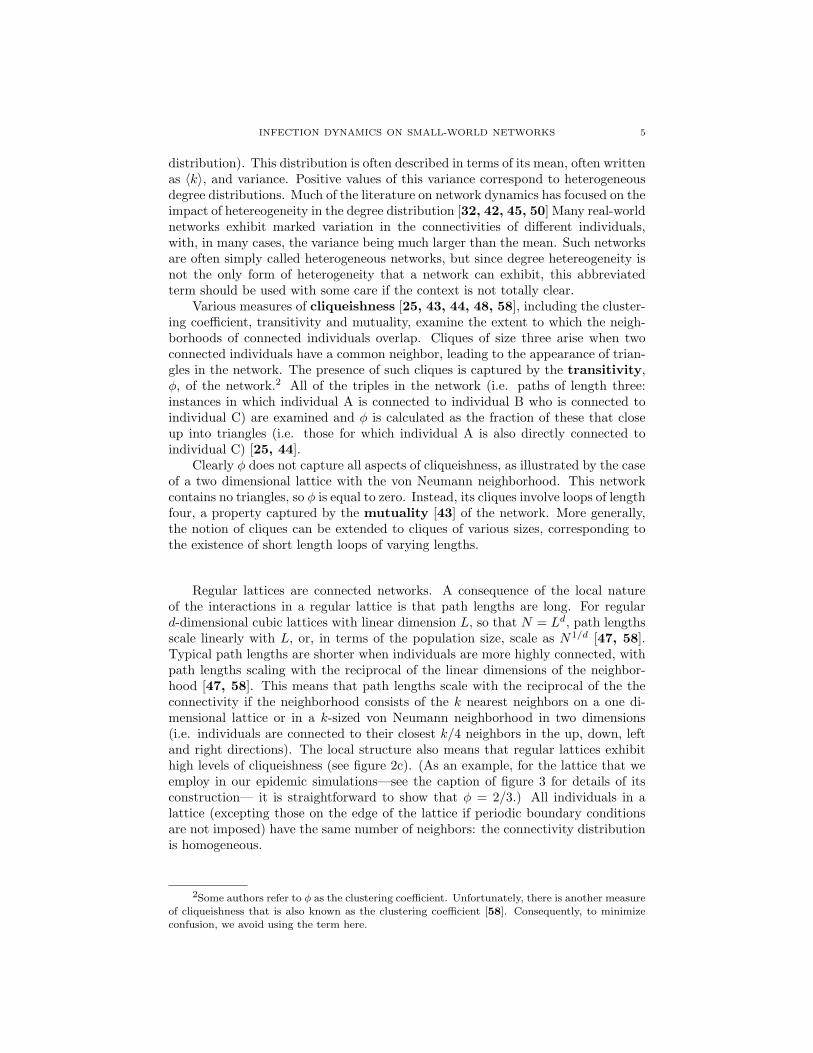
Various measures of cliqueishness [25, 43, 44, 48, 58], including the cluster-ing coefficient, transitivity and mutuality, examine the extent to which the neigh-borhoods of connected individuals overlap. Cliques of size three arise when twoconnected individuals have a common neighbor, leading to the appearance of trian-gles in the network. The presence of such cliques is captured by the transitivity,φ, of the network.2 All of the triples in the network (i.e. paths of length three:instances in which individual A is connected to individual B who is connected toindividual C) are examined and φ is calculated as the fraction of these that closeup into triangles (i.e. those for which individual A is also directly connected toindividual C) [25, 44].

Clearly φ does not capture all aspects of cliqueishness, as illustrated by the caseof a two dimensional lattice with the von Neumann neighborhood. This networkcontains no triangles, so φ is equal to zero. Instead, its cliques involve loops of lengthfour, a property captured by the mutuality [43] of the network. More generally,the notion of cliques can be extended to cliques of various sizes, corresponding tothe existence of short length loops of varying lengths.

Regular lattices are connected networks. A consequence of the local natureof the interactions in a regular lattice is that path lengths are long. For regulard-dimensional cubic lattices with linear dimension L, so that N = Ld, path lengthsscale linearly with L, or, in terms of the population size, scale as N1/d [47, 58].Typical path lengths are shorter when individuals are more highly connected, withpath lengths scaling with the reciprocal of the linear dimensions of the neighbor-hood [47, 58]. This means that path lengths scale with the reciprocal of the theconnectivity if the neighborhood consists of the k nearest neighbors on a one di-mensional lattice or in a k-sized von Neumann neighborhood in two dimensions(i.e. individuals are connected to their closest k/4 neighbors in the up, down, leftand right directions). The local structure also means that regular lattices exhibithigh levels of cliqueishness (see figure 2c). (As an example, for the lattice that weemploy in our epidemic simulations—see the caption of figure 3 for details of itsconstruction— it is straightforward to show that φ = 2/3.) All individuals in alattice (excepting those on the edge of the lattice if periodic boundary conditionsare not imposed) have the same number of neighbors: the connectivity distributionis homogeneous.

2Some authors refer to φ as the clustering coefficient. Unfortunately, there is another measureof cliqueishness that is also known as the clustering coefficient [58]. Consequently, to minimize

confusion, we avoid using the term here.


a) b)

A

B

c)

Figure 2. Network Properties. (a) and (b) Path lengths are longin the regular lattice, but are rapidly shortened with the inclusionof long-range links. (c) Cliques are common in regular lattices.In this example, we focus on two individuals, A and B, who areconnected. We see that four individuals are neighbors of both Aand B. Notice that these cliques correspond to the occurrence oftriangles in the network.

Random graphs are not necessarily connected. If the connection probability,q, is small then the graph is typically composed of a large number of small, dis-connected components [10]. The distribution of the sizes of these components isexponential with finite mean, even as N tends to infinity. These sizes are O(1),which means that they do not scale with N (provided that N is sufficiently large).When q is sufficiently large, the random graph typically consists of one connectedsubgraph that includes a large fraction of the population, together with a number ofsmall disconnected components. This component is known as the ‘giant component’of the graph and its size is O(N) (that is to say, the size of the giant componentscales linearly with N : notice that the average number of nodes, therefore, divergesas N →∞, but that average fraction of nodes in the giant component approaches aconstant). The size distribution of the remaining small components is exponential,with finite mean. Again, these sizes are O(1). A well-known theorem [10] makesthese statements more precise, stating that (for N → ∞) the random graph hasa (single) giant component if and only if Φ = Nq is greater than one. (We shallsee that Φ is simply the average connectivity of the nodes in the network). Thiscomponent then contains a proportion z of the population, where z is the greatestroot of the equation

z = 1− exp(−Φz).(1)

The global nature of mixing in random graphs means that distances are shortcompared to those in regular lattices. Path lengths scale with the logarithm of the


population size and with the reciprocal of the logarithm of the average connectivity[58]. Cliques are rare in random graphs, with φ scaling as 1/N for large N [45, 58].The connectivity distribution of the random graph is binomially distributed, accord-ing to B(N − 1, q). For large N this distribution approaches a Poisson distributionwith mean (N − 1)q ≈ Nq. Since the variance and mean are equal for Poissondistributions, the variance of the connectivity distribution equals Nq. We remarkthat the connectivity distribution of the random graph is not very heterogeneous:few nodes have connectivity that differ that greatly from the average.

For small values of the rewiring parameter, p, (or for a small frequency ofadditional links) most of the links in the small-world network are simply those ofthe lattice and there are only a few long range connections. The surprising result ofWatts and Strogatz is that these few long-range connections rapidly shorten pathlengths in the network. As the parameter p is increased, path lengths quickly fall tobecome comparable to those in the random graph [58]. Cliqueishness, on the otherhand, is much less affected by rewiring: it is not until p takes values approachingone that the remnants of the highly clustered lattice are destroyed by rewiring.For a wide range of p values, the Watts and Strogatz algorithm generates networksthat have the short path length of the random graph while having the high level ofcliqueishness of the lattice: this is the small-world regime. Small-world networks,in this sense, exhibit both local and global mixing properties.

0.0001 0.001 0.01 0.1 1Rewiring probability, p

0

0.2

0.4

0.6

0.8

1

Rela

tive

path

leng

th,

Rela

tive

trans

itivi

ty

Figure 3. Path lengths and cliqueishness in small-world networks.Small-world networks were generated using the Watts and Stogatzmethod [58]. Starting from a one dimensional lattice of 1000 indi-viduals, each of which were connected to their ten nearest neigh-bors, links were rewired using the rewiring technique discussedin the text. Periodic boundary conditions were assumed. Thesolid curve with squares shows the dependence of the average pathlength, relative to the average path length of the unrewired lattice,on the per-link rewiring probability, p. The broken curve with cir-cles shows the cliqueishness, as measured by the transitivity (φ),relative to that of the unrewired lattice, which equals 2/3. Eachpoint on the figure represents the average value taken over 200realizations of the rewired network.


The heterogeneity of the small-world networks generated using the Watts-Strogatz method is intermediate between those of the lattice and the random graph.In the p = 1 case, the degree distribution of the Watts-Strogatz graph generatedusing their original algorithm (in which only one end of each link is rewired, withthe fixed end being chosen systematically) has a lower variance than that of thePoisson distribution of the random graph [5]. In this respect, their totally rewiredgraph differs from the random graph3. The rewiring algorithm that we employ, inwhich both ends of links are rewired, leads to a degree distribution that is closer tothat of the random graph. (The resulting graph is still not quite the Erdos-Renyirandom graph described earlier, since the total number of links in the network isfixed.) In none of these cases, however, is the variance particularly large and soheterogeneity of the degree distribution will not play a major role in the dynamicsof infection on the graphs considered here.

We remark that many networks with heterogeneous degree distributions also ex-hibit short average path lengths [13]. Here, we restrict use of the term ‘small-worldnetwork’, and our attention, to the Watts-Strogatz type of small-world network.

3. Analysis Techniques and Basic Properies

We first consider a particularly simple infection process. Individuals are as-sumed to be initially susceptible to the infection. An infectious individual cantransmit infection to a susceptible; we assume that, once infected, the person isinfectious immediately. Over time, infectious individuals can recover and it is as-sumed that recovery confers permanent immunity to the infection. This descriptionof infection is known as the SIR (susceptible/infectious/recovered) process [1, 14].

It is typically assumed that there is a constant rate of transmission between aninfective and susceptible who are in contact, and that this rate is the same for allsuch infective/susceptible pairs. Writing this transmission rate as β, we have thatthe probability of transmission in the short time interval (t, t + dt) is equal to β dt.The recovery process can be described in many different ways, but most often it iseither assumed that recovery occurs at a constant rate, γ, or that recovery occurs atsome fixed time, τ , after infection. The constant recovery rate assumption leads tothe distributions of infectious periods being exponentially distributed, with meanequal to 1/γ. In order to compare the two descriptions of recovery, the values of τand 1/γ are taken to be the same.

3.1. Well-Mixed Population-Level Models. A familiar population-leveldescription of the SIR process in a well-mixed population, assuming a constant rateof recovery, is given in terms of the following set of differential equations [1, 14]

x = −cbxy(2)y = cbxy − γy(3)z = γy.(4)

Here x, y and z denote the fractions of the population who are susceptible, infectiousand recovered, respectively. In this formulation, the parameter c is the rate at which

3Also recall the earlier comment that the original Watts and Strogatz algorithm guarantees

that each node has connectivity at least 〈k〉/2. The resulting network—even when fully rewired—is guaranteed to remain connected. In contrast, the rewiring algorithm that we employ in this

paper can lead to nodes becoming disconnected.


an individual makes contacts with others and the parameter b is the probabilitythat a given contact (if made between an infective and susceptible) would leadto transmission of the infection. This formulation assumes that the population isclosed: no individuals leave or enter the population, so one need not worry aboutdemographic processes. As a consequence, equation (4) is redundant: becausean individual is either susceptible, infectious or recovered, one can calculate z as1− x− y.

The behavior of this deterministic model is well known [1, 14]. Since thereis no replacement of susceptibles, introduction of infection either leads to a singleoutbreak, which is self-limited due to the ensuing depletion of susceptibles, or nooutbreak occurs. A threshold condition governs the occurrence of these alternatives:if the value of the so-called basic reproductive number, R0, is greater than one thenan epidemic can occur, otherwise the number of infectives can never increase.

The basic reproductive number can be written in terms of model parametersas

R0 = cb/γ,(5)

and has a simple epidemiological interpretation. For the initial stages of the epi-demic, when almost the entire population is susceptible, the parameter c gives therate at which an individual, in particular an infective person, encounters susceptibleindividuals. Since 1/γ is the average duration of infection, c/γ gives the averagenumber of susceptibles encountered over their infectious period. As the product ofthe average number of susceptibles encountered and the transmission probability,R0 gives the average number of secondary infections that arise when an infectiousindividual is introduced into an otherwise entirely susceptible population. In thiswell-mixed deterministic setting, and in the absence of demography, the value ofthe basic reproductive number does not depend on the distribution of infectiousperiods: R0 reflects the average number of secondary infections rather than thetiming of their occurrence.

The total fraction of people who are infected over the course of the entireepidemic, which we call the size of the epidemic and write as y∞, is given by thelargest root of the following equation

y∞ = 1− exp (−R0y∞) .(6)

If R0 is greater than one then this quantity is positive.In the preceding discussion, we deliberately used different parameterizations for

the transmission processes in well-mixed settings and in network settings. Manystudies have compared infection dynamics in these two settings, in which case onemust be able to move between the two parameterizations in order to make com-parisons. In such studies, the parameter combination cb is typically identified withβk [25, 27]. Use of the well-mixed description, together with this identificationof parameters, leads to the expression R0 = βk/γ, or R0 = βkτ , for the basicreproductive number for random networks4. As we shall see below, more careful

4This expression ignores all sources of heterogeneity in the network, including heterogeneity

in the connectivity distribution. Degree heterogeneity can be accounted for in the differential

equation framework by subdividing the population into subgroups according to individuals’ con-nectivities. Use of this approach has led to the development of analogous expressions for R0 that

account for heterogeneity in the degree distribution [32, 50].


consideration shows that this expression is incorrect in a couple of important waysfor network settings.

3.1.1. Stochastic Models in Well-Mixed Settings. The deterministic models ofthe previous section treated the numbers of susceptible, infectious and recoveredindividuals as continuously varying quantities, whose changes could be describedby a set of differential equations. In reality, the numbers of individuals of differenttypes are integers, and change discretely as infection or recovery events occur. Thefinite size of a population and the ensuing stochastic effects (known as demographicstochasticity) can be accounted for using stochastic formulations of the well-mixedmodel (see, for example, [2]).

The stochastic well-mixed model also exhibits threshold effects as the basicreproductive number, which is again given by equation (5), is increased from belowto above one [2, 14]. Below the threshold, each infective gives rise to an averageof fewer than one secondary infection and so introduction of a single infective (ora small number of infectives) can only give rise to a minor outbreak. It shouldbe noted that some of these ‘minor’ outbreaks can involve a significant number ofindividuals: even though the average number of secondary infections is less thanone, chance events can lead to a few individuals having many more secondaryinfections than this.

Above the threshold, introduction of infection can lead to a major outbreak,potentially affecting a large fraction of the population. Large outbreaks are not,however, guaranteed to occur since it is possible for an infective to recover beforepassing on the infection. Stochastic extinction can occur if this happens for all ofthe infectives present at some point in time: a minor outbreak will occur if thishappens early after the introduction of infection.

Using branching process theory, expressions have been derived for the proba-bilities of the occurrence of major and minor outbreaks when R0 is greater thanone (see, for example, [14]). The most familiar result states that, for the constantrecovery rate model, the probability of a major outbreak occurring following theintroduction of a single infective is 1 − (1/R0). If recovery is instead assumed tooccur at exactly time τ after infection, the probability of a major outbreak, π, isgiven by the largest root of

π = 1− exp(−R0π).(7)

3.2. Percolation and Graph Theory Approaches. The similarity be-tween equation (1) for the size of the giant connected component of a randomgraph and equation (6) for the size of an epidemic in a well-mixed population (and,indeed, equation (7) for the probability of a major outbreak) is no coincidence.The corresponding threshold conditions for the connectedness of the random graph(average connectivity greater than one) and the R0 = 1 threshold (average numberof secondary infections greater than one) are also similar to each other5. Noted byBarbour and Mollison [4], questions concerning epidemic processes on networks canbe rephrased in terms of questions about the properties of graphs. As Barbour andMollison point out, this means that the body of theory developed to describe the

5There are also clear analogies between the preceding discussions of the component size dis-tribution of the random graph and the occurrence of minor and major outbreaks in the stochastic

well-mixed model.


properties of graphs is informative about epidemic processes that occur on thosegraphs. One such approach that has been fruitfully applied is percolation theory.

The bond percolation problem on a graph [22] assumes that each edge in thegraph can independently be traversed with some probability, q. Percolation theorythen addresses questions such as the extent to which the network can be traversed.The earliest percolation studies focused on regular lattices and so the nature ofpercolation on such lattices has been described quite fully [22]. Following theintroduction of small-world networks, their percolation properties have been char-acterized in detail [37, 38, 41, 46].

We note that the construction of a random graph can be described in terms ofthe bond percolation problem by starting with a completely connected graph andthen taking the traversal probability of each edge of the connected graph to be q.

Grassberger [21], assuming that transmission rates were equal along each edgein the network and that individuals had a fixed duration of infection, noted thatthe spread of infection on a graph could also be mapped onto the bond perco-lation problem. In this simple epidemiological setting the correspondence withbond percolation is intuitively clear: transmission along an edge occurs with someprobability, known as the transmissibility, which we then interpret as the traversalprobability in the bond percolation model. We can then follow the infection spread-ing across the network and ask about the size of the network component that canbe reached from the initial infective if one follows edges along which transmissionoccurs. (We remark that not all traversable edges in the bond percolation modelwill correspond to transmission events. Only traversable edges that can be reachedfrom the initial infective can be interpreted in this way; the extra edges are not ofinterest in the infection context.)

Sander and co-workers [54] generalized this approach to a broad class of epi-demic models. Newman [42] gives a lucid description of the correspondence be-tween epidemic spread and percolation. Since the percolation problem is, for agiven network, formulated solely in terms of the probability of transmission alongedges (assuming that one node is infective and the other susceptible), the rates oftransmission along edges and the durations of infection of nodes need not all be thesame. Newman argues that the percolation approach can be applied to any settingin which these quantities are independent, identically distributed quantities, sincethen the probabilities of transmission are, a priori , equal along all edges. In suchsituations, the transmissibility is calculated by averaging over the distribution ofinfectious periods and the distribution of transmission rates [42]. This argumentdoes not hold when, for instance, transmission rates and/or infectious periods aredrawn from different distributions for different edges and/or nodes and the result-ing transmission probabilities differ between edges. Newman [42] shows that thepercolation approach can still be useful even in some such instances, although theproblem is no longer described in terms of a single transmissibility.

For the simple SIR processes introduced at the start of section 3, the transmis-sibility depends on the transmission rate along edges, β, and the infectious perioddistribution. If the duration of infection, τ , is the same for all individuals, we havethat T = 1 − exp(−βτ) [27, 42]. For the constant recovery model (exponentiallydistributed infectious periods with mean τ), averaging over the infectious perioddistribution gives T = βτ/(1 + βτ) [27].


We notice that if the product βτ is small compared to one, then either of theabove expressions for T can be well approximated by βτ . Intuitively, this makessense since the product of the per-link transmission rate and the average durationof infection will approximately equal the transmission probability along the link,provided that this product is not too large. (That βτ is just an approximation tothe transmission probability is immediately clear since it can take values greaterthan one.)

3.2.1. Percolation Theory and Epidemic Thresholds. The results of percolationtheory show that threshold behavior is typical in these systems. As in the earlierdiscussion of the construction of the random graph, there is a critical value of thetraversal probability, below which the traversable network consists of a large num-ber of small components, which are of size O(1), and above which the traversablenetwork consists of a single giant component, of size O(N), and a number of smallcomponents. In the epidemiological interpretation, there is a critical value of thetransmissibility, below which only minor outbreaks occur and above which eithermajor or minor outbreaks can occur. A major outbreak will occur if the initialinfective is located in the giant component, and a minor outbreak will occur if theinitial infective is located in one of the small components. The probability of theoccurrence of a major outbreak, therefore, is equal to the fraction of nodes that arefound within the giant component. This threshold behavior is precisely that of theepidemiologically familiar R0 = 1 threshold, as described above in the case of thewell-mixed stochastic model.

Percolation theory can be used to quantify the threshold and give a detailedaccount of behavior near the threshold (so-called ‘critical behavior’), in additionto yielding information about the probability distribution of outbreak sizes andthe probability of the occurrence of an outbreak. For example, Grassberger [21]describes power law (scaling) behavior in the outbreak probability when the trans-missibility is just above the threshold, and in the outbreak size distribution whenthe transmissibility is just below threshold (see also [53]).

One important difference between network settings and the population-levelwell-mixed models is that individuals have a fixed set of contacts. This leads tosome important differences in the expression for the basic reproductive number,even for the random graphs that attempt to model well-mixed settings. If, in alarge well-mixed population (i.e. a random network), every individual is assumedto have exactly k neighbors, and it is assumed that there are no loops of shortlength in the network, then the basic reproductive number is given by [14, 15]

R0 = T (k − 1).(8)

In the language of percolation theory, there is a critical value of the transmissibility,given by TC = 1/(k − 1), above which large outbreaks can occur [42].

Notice that R0 depends on the number of neighbors minus one. Every indi-vidual who transmits infection, except for the initial infective, can have at mostk − 1 susceptible neighbors because they must have acquired infection from oneof their neighbors. Also notice that the value of the basic reproductive numbernow depends on the infectious period distribution, although this dependence willbe weak if βτ is small.

It is instructive to compare expression (8) to the simple-minded expressionR0 = βkτ obtained using the population-level well-mixed model. Two differencescan be seen: the latter involves k and not k− 1, and, since βτ can be greater than


one, the average number of secondary infections can exceed k. These deficienciesarise because the well-mixed model does not account for individuals having a finitenumber of neighbors.

Using branching process theory, Diekmann and co-workers [14, 15] derived aformula for the average final size of a major outbreak in the k-neighbor randomgraph described above. If R0 is greater than one, it can be shown that the followingequation for θ

θ = (1− T + θT )k−1(9)

has a unique root in (0, 1). Diekmann et al. then showed that the final size of theepidemic (i.e. the fraction ever infected), y∞, is given by

y∞ = 1− (1− T + θT )k.(10)

As discussed earlier, y∞ also gives the probability of the occurrence of a majoroutbreak. In the limit as k → ∞, if β is scaled inversely with the connectivity6,Diekmann et al. note that equation (6) is recovered.

Clique structure also impacts the spread of infection [8, 25, 44], since it reducesthe number of secondary infections that each individual can cause. Using figure 2cas an example, imagine that individual A is the initial infected individual andthat they infect person B. Although both individuals still have seven susceptibleneighbors, four of these neighbors are shared and so the maximum number of furthersecondary infections is just ten. From the viewpoint of transmission, localizedinteractions mean that there are a large number of wasted contacts. Consequently,the value of the basic reproductive number is lower than in comparable well-mixedsettings. This leads to outbreak sizes being smaller in cliqueish networks [25, 44],although Newman points out the counterintuitive result that cliqueishness can makeit easier for these smaller outbreaks to occur when the transmissibility is low [44].

Threshold values of the transmissibility for lattices and small-world networkscan can be obtained using percolation results. As mentioned above, percolationon regular lattices has received much attention and so critical values are knownfor many bond percolation problems. For the two dimensional lattice with the vonNeumann neighborhood (i.e. connections are made to the four nearest neighbors),it is known that the percolation threshold occurs at q = 1/2 [22]. The percolationproblem on small-world networks has also received much attention [37, 38, 41, 46].Moore and Newman [37, 38] provide solutions for the bond percolation problemson one dimensional small-world networks for which connections are made either tothe nearest neighbors or the two nearest neighbors on either side of each individual.They point out that their approach could be extended to more highly connectedsettings, but that the calculations rapidly become more involved as k increases. Itshould also be pointed out that they describe their approach for the variant small-world generating algorithm in which long-range links are added in addition to thoseof the lattice, rather than the rewiring approach that we adopt here.

Heterogeneity of the network’s degree distribution impacts the spread of infec-tion. A well-known formula, appropriate for a particular mixing pattern known asproportionate mixing, illustrates how heterogeneity inflates the basic reproductive

6This corresponds to the notion that as a person makes contacts with more people, they willspend less time in contact with each of them: their infectivity is diluted across their neighbors.

This corresponds to the formula cb = kβ discussed in Section 3.1.


number [14, 35, 42]:

R0 = T

(〈k〉 − 1 +

Var(k)〈k〉

).(11)

Here 〈k〉 and Var(k) denote the mean and variance of the degree distribution,respectively. Many real-world networks have highly heterogeneous degree distri-butions: in such instances, the expression for the basic reproductive number maybe dominated by the variation in the degree distribution, rather than its average.As mentioned earlier, the small world networks that are the focus here are fairlyhomogeneous: the issue of heterogeneity is not an important concern for this study.

3.3. Pair Models. Percolation theory is not the only approach that has beenused to address questions such as whether an infection can spread on a given net-work, the resulting outbreak size distribution or the temporal dynamics of thisspread.

Infection spreads less rapidly on a typical network than it would in a well-mixed population. In the latter, a single infective can directly infect any susceptibleindividual because everyone interacts with everyone else in the population. Unlessthe network is completely connected, each individual will have fewer than N − 1neighbors, and so infection must travel via intermediate individuals in order toreach everyone in the population.

In contrast to well-mixed settings, transmission rates for general networks can-not be adequately described just in terms of the numbers of susceptibles and in-fectives. Rates of transmission depend on the configuration of these susceptiblesand infectives, depending on the number of instances in which a susceptible isfound to be in contact with an infective individual: we might term these instancessusceptible-infective pairs.

a) b)

Figure 4. Spread of infection depends on the configuration ofpairs. The network fragments in both (a) and (b) have five suscep-tibles (unshaded circles) and one infective (shaded circle). Infectionwill clearly spread more rapidly in (b) than in (a) because the singleinfective is connected to more susceptibles. In (a), we have four S-S (susceptible-susceptible) pairs and one S-I (susceptible-infective)pair, whereas in (b) we have five S-I pairs.

Pair models [8, 18, 25, 52, 55] attempt to capture this structure, keepingtrack of the numbers of pairs in which individuals of different types are connected.Differential equations then describe how the numbers of the different types of pairs


change over time. Keeling [25] derives the following set of equations for the dy-namics of pairs for the SIR process

˙[SS] = −2β[SSI](12)˙[SI] = β ([SSI]− [ISI]− [SI])− γ[SI](13)˙[SR] = −β[RSI] + γ[SI](14)˙[II] = 2β ([ISI] + [SI])− 2γ[II](15)˙[IR] = β[RSI] + γ ([II]− [IR]) .(16)

Here, the number of X-Y pairs is denoted by [XY ], where X and Y can denote S, Ior R type individuals. For book-keeping reasons, [XX] denotes twice the numberof X-X pairs. The number of X-Y-Z triples is written as [XY Z]. Notice that it isnot necessary to have equations that track the numbers of individuals of each type,which in Keeling’s notation would be denoted [X]: these quantities can alwaysbe calculated in terms of the numbers of pairs involving the type of interest. Forexample, the number of susceptible individuals can be calculated if the numbers ofS-S, S-I and S-R pairs are known.

One feature of these equations is that the rates of change of pairs involve theconfiguration of triples. If one looked at equations for triples, one would find thatthey involve quartets, and so on. In order to usefully employ this approach, theset of equations is truncated (or closed) at some order. One way to do this is viaso-called pair approximations, in which the configuration of triples is described, inan approximate way, in terms of the configuration of pairs. This then eliminatesthe need for equations that describe how the numbers of triples evolve over time,leaving a closed set of equations for the numbers of pairs. We remark that theuse of the pair approach for this SIR process replaces a two dimensional model,equations (2) and (3) by a five dimensional system.

Various pair approximations can be made, reflecting the geometry of the net-work. A different approximation would be more suited to graphs that are similarto random graphs than would be appropriate for ones that are similar to lattices.Keeling [25] considers graphs for which each individual has k neighbors and thatare further specified in terms of their cliqueishness, as measured by the transitivity,φ. He uses the following approximation

[ABC] ≈ k − 1k

[AB][BC][B]

((1− φ) + φ

N

k

[AC][A][C]

),(17)

first described by Morris [39], to close the set of moment equations, where N isthe population size. Bauch [8] calls this the triangular pair approximation, since itaccounts for the occurrence of triangles in the network. The accuracies of variouspair approximations in lattices with various different geometries are discussed byBauch [8], in which it is pointed out that the standard pair approximation often doesnot provide a completely satisfactory description. (For this reason, the predictionsmade by pair models are almost invariably compared to those obtained by numericalsimulation of the full network model.)

A number of techniques are available that extend these pair models [7, 8,18], including extending the set of equations to account for the configuration oftriples [7, 8]. Alternatively, in a disease invasion setting, the so-called invasory pairapproximation attempts to account for the structure of the clusters that develop


during the invasion process [8]. Another approach for invasion settings, the pair-edge approximation [18], attempts to describe the leading edge of the invasion wavefront, enabling estimation of the speed at which the infection spreads across thepopulation.

Threshold results can be obtained using pair models, and their extensions, byexamining whether infection can invade a population or not. This question is moredifficult to address in the five dimensional pair model than it is in the standarddeterministic SIR model. This task can be simplified somewhat on account of thespatial structure that quickly develops during the invasion of the infection. Thisallows quasi steady state assumptions to be made, reducing the dimensionality ofthe system and facilitating the calculation of thresholds [8, 18, 25].

The system of pair equations can be integrated, allowing the final size of theepidemic to be calculated. Typically this integration can only be carried out nu-merically.

4. Epidemic Dynamics

The impact of various aspects of network structure on the spread of infection iseasily understood in terms of the preceding discussion. All other things being equal,infection will spread more readily and rapidly when the average connectivity ofindividuals is higher. Highly localized mixing hinders the spread of infection, bothbecause of cliqueishness, which leads to wasted contacts, and because long pathlengths mean that infection must travel through a large number of intermediatesin order to spread across the entire network.

Epidemics on lattices, therefore, spread slowly and exhibit high degrees of spa-tial structure. If infection is introduced at a single location, this spread will takethe form of an outward spreading wave, the speed of which will depend on epi-demiological parameters and the geometry of the lattice. Epidemics on randomgraphs spread much more rapidly and exhibit little or no spatial structure. Epi-demics on small-world networks will be intermediate between these two extremes,and so spread at some intermediate speed. Their spatial structure will involve anumber of growing clusters of infection: the mainly local nature of mixing meansthat there will be wave-like spread out from a point of introduction, but long-rangetransmission events will often take infection to virgin territory, giving rise to newclusters of infection.

Figures 5-7 illustrate several aspects of epidemic dynamics, summarizing theresults of repeated stochastic simulation of the SIR process on graphs generatedby the Watts-Strogatz small-world algorithm. Figure 5 depicts the timecourse ofepidemics, averaged over 1000 realizations of the model, assuming three differentvalues of the Watts-Strogatz per-link rewiring probability. In this figure, the pa-rameter values are chosen so that the transmissibility is quite some way above theepidemic threshold. The spread of infection is much faster in the random graphthan in the lattice. Following a short initial transient, in this case so short that itis barely noticeable on the scale of the figure, the cumulative incidence increaseslinearly with time for a long period in the lattice, reflecting the wave-like spread ofinfection outwards from the point of introduction. The impact of long-range links isdramatic: a rewiring probability of just one percent turns the lattice into a networkon which infection spreads considerably faster.


0 5 10 15time

0

200

400

600

800

1000

Prev

alen

ce o

f inf

ectio

n

0 5 10 15time

0

200

400

600

800

1000

Cum

ulat

ive

inci

denc

e

a)

b)

Figure 5. Averaged timecourse of epidemics on a few of the net-works depicted in figure 3, generated using the Watts-Strogatzmethod, under the SIR infection process assuming that β = 1.0and that each infection lasts exactly one time unit (i.e. τ = 1).The upper panel depicts the prevalence of infection (i.e. the num-ber of infectious people at each point in time) and the lower paneldepicts the cumulative incidence (i.e. the total number of casesup to the time point). The solid curves illustrate simulations onthe lattice (p = 0), and the dashed curves illustrate simulationson the random graph generated by rewiring all the links of thelattice (p = 1). The dotted curves denote the intermediate case ofa small-world network, with just one percent of the lattice’s linksbeing rewired (p = 0.01). Curves are calculating by averaging over1000 realizations of the model.

An interesting observation [29] is that the timecourse of the epidemic in thesmall-world regime echoes that of a standard SIR model, albeit with different valuesof its parameters. This idea has recently been taken up by Aparacio and Pascual(manuscript in prep.) who modify a standard SIR model to capture some of thefeatures of spatial structure, such as the local depletion of susceptibles within infec-tion clusters, providing a description of the epidemic in terms of a low dimensionaldynamical system.

Figure 6 illustrates the distribution of outbreak sizes that are seen when a singleinfective is introduced into an otherwise susceptible population. The parametervalues in figure 6 are chosen to be closer to the epidemic threshold than thoseof the previous figure, with the transmissibility of this infection equalling T =1 − exp(−0.2) ≈ 0.181. In the k-neighbor random graph setting, expression (7)gives R0 ≈ 1.63: this value is not so far above the epidemic threshold.


0 200 400 600 800 1000outbreak size

0

500

1000

1500

2000

frequ

ency

0 25000 500000

1000

2000

0 200 400 600 800 1000outbreak size

0

500

1000

1500

2000

frequ

ency

0 200 400 600 800 1000outbreak size

0

500

1000

1500

2000

frequ

ency

0 200 400 600 800 1000outbreak size

0

500

1000

1500

2000

frequ

ency

a) b)

c) d)

Figure 6. Outbreak size distributions for the SIR infection pro-cess on the networks of figure 3, assuming that β = 0.2 and thateach infection lasts exactly one time unit (τ = 1). In each case, theaverage connectivity of the network is ten and the network consistsof 1000 individuals. In panel (a), no links are rewired. Panels (b)and (c) use small-world networks generated from the underlying1D lattice with per-link rewiring probabilities equal to 0.040 and0.079. All links are rewired in the network of panel (d). The in-set in panel (b) shows the corresponding outbreak size distributionwhen the network contains 100 000 individuals (with p still equalto 0.040). Each panel depicts the outcomes of 10000 realizationsof the model, but for clarity the vertical axis is cut off at 2000.(In each case, the peak corresponding to ten or fewer cases reachesabove this cut-off.)

For the parameter values in figure 6, rewiring the lattice has moved the pop-ulation from being below the epidemic threshold to above the epidemic threshold.For the lattice (figure 6a), we see that introduction of infection only leads to a mi-nor outbreak, whereas for the corresponding small-world network (if p is sufficientlylarge), or the random graph obtained when all links are rewired, introduction eitherleads to a minor outbreak or a major outbreak. The histograms in figures 6c and6d are clearly bimodal, comprising two components: the exponentially boundeddistribution of minor outbreaks and the distribution of major outbreaks.

As in our earlier discussion of the stochastic well-mixed model, we see that,even above the epidemic threshold, introduction of infection does not guarantee theoccurrence of a major outbreak. Use of equations (9) and (10) gives the averagesize of the major outbreaks (i.e. the fraction of the population that is affected) that


result from the introduction of a single infective into a k-neighbor random graph,and, equivalently, the probability of the occurrence of a major outbreak, as ≈ 0.749.This is very close to the 74% of simulations that give rise to a major outbreak infigure 6d (see also figure 7, panel b). (It should be noted that the network onwhich the simulations are run in figure 6d does not correspond exactly to the onedescribed by Diekmann et al., since the random rewiring means that there will besome (small) heterogeneity in the degree distribution.)

From the histograms of figure 6, we see that increasing the rewiring probabilityincreases the probability of the occurrence of a major epidemic and increases theaverage size of the ensuing outbreak. We also notice that the distribution of the sizesof the major epidemics becomes less variable as the rewiring probability increases.Close to the threshold, we see a transition regime in which the distinction betweenminor and major outbreaks is less clear: the histogram in figure 6b is less clearlybimodal than one obtained further above the threshold (for example, figure 6c).Since the minor outbreaks are of size O(1) and the major outbreaks are of sizeO(N), this transition regime is less noticeable when N is larger. This is illustratedin the inset to panel (b), obtained for the same value of p but with a population sizethat is one hundred times larger. Comparison between the main graph of panel (b)and its inset also illustrates that the sizes of the major outbreaks are more closelycentered around their mean for large population sizes (see [2] for a more completediscussion of this effect).

Figure 7a clearly illustrates the threshold behavior of the model as the rewiringprobability is increased. Also visible is the O(N) behavior of the sizes of themajor outbreaks, with the fraction of the population ever infected above thresholdbeing independent of N (main graph). The O(1) behavior of the sizes of minoroutbreaks is also clear, with the number of people ever infected below thresholdbeing independent of N (inset graph).

Figure 7b depicts, in terms of the rewiring parameter, the average outbreak size(calculated across all realizations, regardless of whether a minor or major outbreakoccurred), the probability of the occurrence of a major outbreak and the size ofthe ensuing major outbreak, if it occurs. (Put another way, the last quantity isthe average outbreak size conditional on the occurrence of a major outbreak.) Asexpected, the probability of the occurrence of a major outbreak is, within theaccuracy of the simulations, equal to the (fractional) size of a major outbreak forvalues of p above threshold. The transition region around the threshold imposessome difficulties in the estimation of the probability and size of major outbreaks infigure 7b. Since threshold behavior is sharper for larger values of N , as explained inthe discussion of figure 6b and its inset, these difficulties are mitigated by employinglarger population sizes (hence the use of N = 1000 in figure 6 and N = 10000 infigure 7b).

5. Dynamics in Endemic Settings

The assumptions of lifelong immunity and the neglect of demographic pro-cesses are unrealistic for many infections. In many instances, replenishment of thesusceptible population, either with the waning of immunity or the birth of new sus-ceptibles, has a major impact on the dynamics of the infection. Most importantly,this process can lead to the establishment of an equilibrium of infection in whichthe rate at which susceptibles are infected balances the rate at which susceptibles


0.001 0.01 0.1 1Rewiring probability, p

0

0.1

0.2

0.3

0.4

0.5

0.6

Frac

tion

of n

odes

infe

cted

0.001 0.01p

0

50

100

150

200

Num

ber I

nfec

ted

N = 1 000N = 10 000N = 100 000

0.001 0.01 0.1 1Rewiring probability, p

0

0.2

0.4

0.6

0.8

Out

brea

k siz

e

0

0.2

0.4

0.6

0.8

Prob

. of m

ajor

out

brea

k

a)

b)

Figure 7. Panel (a): Dependence of the average fraction ofnodes that ever become infected (main graph) and the averagenumber of nodes that ever become infected (inset graph), follow-ing the introduction of a single infective individual, on the rewiringprobability in the Watts-Strogatz small-world network algorithm.Networks are generated as in figure 3, with population sizes ofN = 1000 (solid line with squares), N = 10000 (solid line withfilled triangles) or N = 100000 (dashed line with circles). Infec-tion parameters are β = 0.2 and τ = 1. Averages were taken over10 000 realizations for N = 1000 and N = 10000, but over 1000realizations for N = 100000. Panel (b) depicts, in terms of therewiring probability, three quantities: the average outbreak size(solid curve with squares), the probability of the occurrence of amajor outbreak (dashed curve) and the average size of a majoroutbreak, if one occurs, (circles). All curves in panel (b) are cal-culated using the simulations shown in panel (a) for N = 10000.Notice that the ‘average size’ curve is calculated by averaging overall realizations of the model (regardless of whether they involveda minor or a major outbreak), and thus corresponds to one of thecurves in panel (a).

are recruited and the rate at which individuals become infected balances the rateat which they recover [1, 14].

Modeling demographic processes requires the removal of individuals from thenetwork upon their death and the insertion of individuals as they are born. Unlessone simply replaces a dying individual by a newborn, this raises questions as towhere newborns should be placed in the network. From the viewpoint of network


settings, therefore, it is much easier to model the replenishment of susceptibles byallowing immunity to wane. The SIRS model assumes that recovered individualslose their immunity at some point. A limiting case of the SIRS model is the SISmodel, in which the duration of immunity is simply set equal to zero: individualsrecover to a susceptible state. On the other hand, if the duration of immunity isallowed to tend to infinity, individuals never recover and the SIRS model approachesthe SIR model.

For simple well-mixed models, there are many similarities between the behav-ior of SIR and either SIS or SIRS infection processes. Most notably, the thresholdconcept carries over to these processes, with the basic reproductive number de-termining a disease invasion condition: introduction of infection can lead to anoutbreak when the basic reproductive number is greater than one. In addition,the same condition ensures the existence and stability of an endemic equilibrium(i.e. one with a positive prevalence of infection) of the system [1, 14, 43]. Inother words, the R0 = 1 condition is also a disease persistence threshold. For manymodels, the expression for R0 is identical in both epidemic (e.g. SIR) and endemic(e.g. SIRS) settings.

In non well-mixed models, the invasion and persistence thresholds need notbe identical: one scenario under which this can arise involves the occurrence of aso-called “backwards bifurcation” at R0 = 1, and has been the subject of manystudies [11, 17].

The stability of the endemic equilibrium has been of considerable interest: insimple settings, the existence of a (positive) endemic equilibrium guarantees itsstability. This is not always the case, however, and for many models, the endemicequilibrium can become unstable via a Hopf bifurcation, leading to stable oscilla-tions in the prevalence of infection [24].

In stochastic settings, random fluctuations prevent the system from settlinginto an equilibrium. If these fluctuations are large enough, then the infection cango extinct: if the number of infectives falls close to zero, then it is possible forall of them to recover before passing on the infection. This phenomenon is knownas (endemic) fade-out [6]: stochasticity means that an infection may not persisteven though its basic reproductive number is large compared to one. This is animportant aspect of the dynamics of many infections, such as measles, in all but thelargest-sized cities. In spatial settings, fade-out leads to local extinction of infection,but need not link to global extinction of infection if outbreaks in different locationsare desynchronized [9, 40]. Indeed, movement of infectious individuals means thatinfection can be reintroduced into a region where it previously underwent fade-out.Consequently, the population-level persistence of infection depends in an importantway on the synchrony of outbreaks across the population [9, 26].

Much of the discussion of the impact of spatial structure on the dynamics andpersistence of infection has been framed in terms of metapopulation models. Thesequestions have, however, also been investigated within the small-world framework[30, 57].

Kuperman and Abramson [30] investigated the dynamics of an SIRS processon a small-world network. For small values of the Watts-Strogatz rewiring param-eter, p, they found that the population-level prevalence exhibited small stochasticfluctuations around an endemic equilibrium. Quite different behavior was seen forlarger values of the rewiring parameter, however, with the prevalence undergoing


large amplitude oscillations. These oscillations occurred on the timescale of theduration of immunity. The change in behavior was accompanied by a change in thesynchrony of outbreaks between different regions of their population.

An intuitive explanation of these results can be given in terms of the mixingpattern of the population and the resulting level of synchrony. For small valuesof p, the mixing is mainly local, and so oscillatory behavior in different localesoccur in an asynchronous fashion. With little synchrony between outbreaks indifferent regions of the population, the population level prevalence undergoes smallamplitude fluctuations about some level: the local oscillations are averaged out atthe level of the whole population (see also [16]). When p is large, mixing is globalin nature and so there is a greater tendency for synchrony between outbreaks indifferent parts of the population. Indeed, the oscillations in prevalence are predictedby a mean-field (well-mixed) model for the system [24].

Verdasca and co-workers [57] considered the persistence and synchrony of out-breaks of an infection such as measles on small-world networks using what theydescribed as an SIR process with demography. (Actually, their model employed anSIRS process since they modeled births by replacing recovered individuals by sus-ceptibles.) Spatial correlations were found to enhance the stochastic fluctuationsaround the endemic equilibrium, with smaller fluctuations in the well-mixed case(p = 1) than when the network was close to a lattice (p ≈ 0).

As noted by Verdasca et al., their study and that of Kuperman and Abramsonmake apparently conflicting predictions regarding the impact of spatial structure onoscillatory behavior. Although some aspects of this conflict are not fully resolved,Verdasca et al. do point out that the two studies examine quite different parameterregimes. Kuperman and Abramson’s study assumes that immunity lasts for a timethat is comparable to the duration of infection; the resulting oscillations are on asimilar timescale. For Verdasca et al., immunity is lifelong, while infection lasts forat most a few weeks; the resulting oscillations are on an intermediate timescale,being on the order of one to three years. Kuperman and Abramson point out thatoscillations are not seen in their model when there is a marked difference betweenthe durations of infectiousness and immunity.

The conventional wisdom in the literature on the metapopulation dynamics ofmeasles is that spatial structure enhances the persistence of infection [9, 26] sinceoutbreak asynchrony can allow global persistence even in the face of frequent localextinction. Persistence is much less likely in a well-mixed population than in a morestructured population. Verdasca et al., however, described an abrupt transition inthe persistence of infection as the rewiring probability, p, was increased. In theirsmall-world model, persistence was much more likely to occur in networks thatwere close to well-mixed. They described this transition in terms of a percolationthreshold and so it appears to be related to the increase in R0 that accompanieshigher values of p, as described in the previous sections. Since it is well-knownthat the invasion threshold is exceeded for measles— indeed with an R0 of about15, measles is highly infectious— this observation of Verdasca et al. does not,unfortunately, address the main question of interest for measles, namely the impactof spatial structure in countering the endemic fade-out effect.

Questions of dynamics and persistence have been considered in other networksettings; these results shed some light on the above studies of small-world settings.Morris [39], discussed by Rand [52], found that the stable endemic equilibrium


of the SIR model gave way to limit cycle behavior on clustered networks as thequantity φ increased through a critical value. We remark that the direction inwhich this change occurs is in agreement with the results of Verdasca et al. Keelingand co-workers [28] demonstrated that clustering in a network could enhance thepersistence of an endemic infection, a finding that is in agreement with the resultsof metapopulation approaches.

6. Discussion

Network models provide a flexible framework within which the impact of popu-lation structure on the transmission dynamics of infections can be studied. On onelevel, they provide a research tool that can be used to investigate the relationshipbetween epidemiological interactions that are described in terms of individuals andtheir behavior, and the resulting population-level patterns of disease transmission.In this way, network models can be used to better understand the assumptionsthat underlie many population-level epidemiological models. On another level, net-work models are being increasingly used as a practical tool, to aid in the analysisof epidemiological data (see [34]), to provide ever more realistic models for real-world populations (see [19]) and to aid in the design of control strategies (see[20, 34, 35, 51])

Although we have framed our discussion within the context of the spatial struc-ture of populations, the network need not correspond to geographic space but ratherto some more general notion of the social space of a population. For instance, mix-ing might be age dependent: for instance, children of the same age are more likelyto spend time together at school [28].

Heterogeneity in the connectivity distribution is an important aspect of thestructure of many populations, but is something we have not discussed here beyondthe mere mention of its existence. As mentioned above, the degree distributions ofthe Watts-Strogatz small-world networks exhibit only low levels of heterogeneity:this class of networks is, therefore, a poor model for many real world populations.It has long been realized, for instance, that sexual partnership networks exhibitextreme heterogeneity (see, for example, [1]), that this heterogeneity has a majorimpact on the spread of infection and that models that ignore this heterogeneitywill provide poor descriptions of reality.

Much of the discussion of network models has been within the context of dis-ease invasion. This setting has long been favored by modelers since invasion isthe setting within which mathematical analysis of epidemic models is often easiest.More recently, real world events have also focused attention on disease invasion:concerns about bioterrorism have fueled the development of models that describethe deliberate introduction of infectious diseases into urban and other settings. Net-work approaches have provided a natural framework for such models [12, 19]. Formany infections, however, the most interesting epidemiological questions concernendemic settings. Although there is an ever growing literature concerning networkapproaches for endemic infections, much work remains to be done here.

7. Acknowledgements

We wish to thank several anonymous referees for their insightful comments,which greatly helped in improving this paper. A.L. and S.V. were supported bythe University of North Carolina Center for AIDS Research (CFAR) by a CFAR


Developmental Award. CFAR is funded by the National Institutes for Health. A.C.-A. was supported by the Department of Mathematics and Statistics of ArizonaState University, the and Statistical and Applied Mathematical Sciences Institute(SAMSI), Research Triangle Park, NC, which is funded by NSF under grant DMS-011209.

References

[1] R. M. Anderson and R. M. May. Infectious Diseases of Humans: Dynamics and Control.

Oxford University Press, Oxford, 1991.[2] H. Andersson and T. Britton. Stochastic Epidemic Models and Their Analysis. Springer, 200.

[3] F. G. Ball, D. Mollison, and G. Scalia-Tomba. Epidemics with two levels of mixing. Ann.

Appl. Prob., 7:46–89, 1997.[4] A. Barbour and D. Mollison. Epidemics and random graphs. In J.-P. Gabriel, C. Lefevre, and

P. Picard, editors, Stochastic Processes in Epidemic Theory, volume 86 of Lecture Notes inBiomathematics, pages 86–89. Springer-Verlag, 1990.

[5] A. Barrat and M. Weigt. On the properties of small-world network models. Eur. Phys. J. B,

13:547–560, 2000.[6] M. S. Bartlett. Deterministic and stochastic models for recurrent epidemics. Proc. 3rd Berke-

ley Symp. on Math., Stat., and Prob., 4:81–109, 1956.

[7] C. T. Bauch. A versatile ODE approximation to a network model for the spread of sexuallytransmitted diseases. J. Math. Biol., 45:375–395, 2002.

[8] C. T. Bauch. The spread of infectious diseases in spatially structured populations: An invasory

pair approximation. Math. Biosci., 2005.[9] B. M. Bolker and B. T. Grenfell. Impact of vaccination on the spatial correlation and persis-

tence of measles dynamics. Proc. Natl. Acad. Sci. USA, 93(22):12648–53, 1996.

[10] B. Bollobas. Random Graphs. Academic Press, 1985.[11] C. Castillo-Chavez, K. Cooke, W. Huang, and S. A. Levin. On the role of long incubation

periods in the dynamics of HIV/AIDS, Part 2: Multiple group models. In C. Castillo-Chavez,editor, Mathematical and Statistical Approaches to AIDS Epidemiology, volume 83 of Lecture

Notes in Biomathematics, pages 200–217. Springer-Verlag, 1989.

[12] G. Chowell and C. Castillo-Chavez. Worst-case scenarios and epidemics. In H. T. Banks andC. Castillo-Chavez, editors, Bioterrorism: Mathematical Modeling Applications in Homeland

Security, volume 28 of SIAM Frontiers in Applied Mathematics. SIAM, 2003.

[13] F. Chung and L. Lu. The average distances in random graphs with given expected degrees.Proc. Natl. Acad. Sci. USA, 99:15879–15882, 2002.

[14] O. Diekmann and J. A. P. Heesterbeek. Mathematical Epidemiology of Infectious Diseases.

John Wiley & Son, Chichester, 2000.[15] O. Diekmann, M. C. M. De Jong, and J. A. J. Metz. A deterministic epidemic model taking

account of repeated contacts between the same individuals. J. Appl. Prob., 35:448–62, 1998.

[16] R. Durrett and S. A. Levin. The importance of being discrete (and spatial). Theor. Popul.Biol., 46:363–394, 1994.

[17] J. Dushoff. Incorporating immunological ideas in epidemiological models. J. Theor. Biol.,180(3):181–7, 1996.

[18] S. P. Ellner, A. Sasaki, Y. Haraguchi, and H. Matsuda. Speed of invasion in lattice populationmodels: pair-edge approximation. J. Math. Biol., 36:469–484, 1998.

[19] S. Eubank, H. Guclu, V. S. A. Kumar, M. V. Marathe, A. Srinivasan, Z. Toroczkai, andN. Wang. Modelling disease outbreaks in realistic urban social settings. Nature, 429:180–184,

2004.[20] N. M. Ferguson, D. A. Cummings, S. Cauchemez, C. Fraser, S. Riley, A. Meeyai, S. Iam-

sirithaworn, and D. S. Burke. Strategies for containing an emerging influenza pandemic insoutheast asia. Nature, 437:209–214, 2005.

[21] P. Grassberger. On the critical behavior of the general epidemic process and dynamical per-colation. Math. Biosci., 63:157–172, 1983.

[22] G. Grimmett. Percolation. Springer-Verlag, 2nd edn. edition, 1991.[23] T. E. Harris. Contact interactions on a lattice. Ann. Prob., 2:969–988, 1974.


[24] H. W. Hethcote, H. W. Stech, and P. Van Den Driessche. Nonlinear oscillations in epidemic

models. SIAM J. Appl. Math., 40:1–9, 1981.

[25] M. J. Keeling. The effects of local spatial structure on epidemiological invasions. Proc. R.Soc. Lond. B., 266:859–67, 1999.

[26] M. J. Keeling. Multiplicative moments and measures of persistence in ecology. J. Theor. Biol.,

205:269–81, 2000.[27] M. J. Keeling and B. T. Grenfell. Individual-based perspectives on R(0). J. Theor. Biol.,

203:51–61, 2000.

[28] M. J. Keeling, D. A. Rand, and A. J. Morris. Correlation models for childhood epidemics.Proc. R. Soc. Lond. B, 264:1149–56, 1997.

[29] A. Kleczkowski and B. T. Grenfell. Mean-field-type equations for spread of epidemics: the

‘small world’ model. Physica A, 274(1-2):355–360, 1999.[30] M. Kuperman and G. Abramson. Small world effect in an epidemiological model. Phys. Rev.

Lett., 86:2909–12, 2001.[31] S. A. Levin and R. Durrett. From individuals to epidemics. Phil. Trans. Roy. Soc. Lond. B,

351:1615–1621, 1996.

[32] R. M. May and A. L. Lloyd. Infection dynamics on scale-free networks. Phys. Rev. E,64:066112, 2001.

[33] J. A. J. Metz, D. Mollison, and F. van den Bosch. The dynamics of invasion waves. In

U. Dieckmann, R. Law, and J. A. J. Metz, editors, The Geometry of Ecological Interactions:Simplifying Spatial Complexity. Cambridge University Press, Cambridge, 2000.

[34] L. A. Meyers, M. E. Newman, M. Martin, and S. Schrag. Applying network theory to epi-

demics: control measures for Mycoplasma pneumoniae outbreaks. Emerg. Infect. Dis., 9:204–10, 2003.

[35] L. A. Meyers, B. Pourbohloul, M. E. Newman, D. M. Skowronski, and R. C. Brunham.

Network theory and SARS: predicting outbreak diversity. J. Theor. Biol., 232:71–81, 2005.[36] D. Mollison. Spatial contact models for ecological and epidemic spread. J. R. Stat. Soc. B,

39:283–326, 1977.[37] C. Moore and M. E. J. Newman. Epidemics and percolation in small-world networks. Phys.

Rev. E, 61:5678–5682, 2000.

[38] C. Moore and M. E. J. Newman. Exact solution of site and bond percolation on small-worldnetworks. Phys. Rev. E, 62:7059–7064, 2000.

[39] A. J. Morris. Representing Spatial Interactions in Simple Ecological Models. PhD thesis,

Warwick University, 1997.[40] G. D. Murray and A. D. Cliff. A stochastic model for measles epidemics in a multi-region

setting. Trans. Inst. Brit. Geog., 2:158–174, 1975.

[41] M. E. Newman, I. Jensen, and R. M. Ziff. Percolation and epidemics in a two-dimensionalsmall world. Phys. Rev. E, 65:021904, 2002.

[42] M. E. J. Newman. Spread of epidemic diseases on networks. Phys. Rev. E, 66:016128, 2002.

[43] M. E. J. Newman. Ego-centered networks and the ripple effect. Social Networks, 25:83–95,2003.

[44] M. E. J. Newman. Properties of highly clustered networks. Phys. Rev. E, 68:026121, 2003.[45] M. E. J. Newman. The structure and function of complex networks. SIAM Rev., 45:167–256,

2003.

[46] M. E. J. Newman, C. Moore, and D. J. Watts. Mean-field solution of the small-world networkmodel. Phys. Rev. Lett., 84:3201–3204, 2000.

[47] M. E. J. Newman and D. J. Watts. Scaling and percolation in the small-world network model.Phys. Rev. E, 60:7332–42, 1999.

[48] M. E. J. Newman, D. J. Watts, and S. H. Strogatz. Random graph models of social networks.

Proc. Natl. Acad. Sci. USA, 99:2566–2572, 2002.

[49] J. V. Noble. Geographic and temporal development of plague. Nature, 250:726–728, 1974.[50] R. Pastor-Satorras and A. Vespignani. Epidemic spreading in scale-free networks. Phys. Rev.

Lett., 86:3200–3, 2001.[51] B. Pourbohloul, L. A. Meyers, D. M. Skowronski, M. Krajden, D. M. Patrick, and R. C.

Brunham. Modeling control strategies of respiratory pathogens. Emerg. Inf. Dis., 11:1249–

1256, 2005.


[52] D. A. Rand. Correlation equations and pair approximations for spatial ecologies. In

J. McGlade, editor, Advanced Ecological Theory: Principles and Applications, pages 100–

142. Blackwell, 1999.[53] C. J. Rhodes and R. M. Anderson. Power laws governing epidemics in isolated populations.

Nature, 381:600–2, 1996.

[54] L. M. Sander, C. P. Warren, I. M. Sokolov, C. Simon C, and J. Koopman. Percolation onheterogeneous networks as a model for epidemics. Math. Biosci., 180:293–305, 2002.

[55] K. Sato, H. Matsuda, and A. Sasaki. Pathogen invasion and host extinction in lattice struc-

tured populations. J. Math. Biol., 32:251–268, 1994.[56] F. van den Bosch, J. A. J. Metz, and O. Diekmann. The velocity of spatial population

expansion. J. Math. Biol., 28:529–565, 1990.

[57] J. Verdasca, M. M. Telo da Gama, A. Nunes A, N. R. Bernardino, J. M. Pacheco, and M. C.Gomes. Recurrent epidemics in small world networks. J. Theor. Biol., 233:553–61, 2005.

[58] D. J. Watts and S. H. Strogatz. Collective dynamics of ‘small-world’ networks. Nature,393:440–2, 1998.

Biomathematics Graduate Program and Department of Mathematics, North Car-

olina State University, Raleigh, NC 27695

E-mail address: [email protected]

Department of Epidemiology, University of North Carolina, School of Public

Health, Chapel Hill, NC 27599E-mail address: [email protected]

Center for Applied Mathematics, Cornell University 657 Rhodes Hall, Ithaca NY

14853E-mail address: [email protected]

Infection Dynamics on Small-World Networksallloyd/pdf_files/small_world.pdf · Infection Dynamics...

Documents

Transcript of Infection Dynamics on Small-World Networksallloyd/pdf_files/small_world.pdf · Infection Dynamics...