INESC-ID TECHNICAL REPORT 1/2004, JANUARY 2004 1 Biclustering … · 2007-12-05 · INESC-ID...

INESC-ID TECHNICAL REPORT 1/2004, JANUARY 2004 1

Biclustering Algorithms for BiologicalData Analysis: A Survey*

Sara C. Madeira and Arlindo L. Oliveira

Abstract

A large number of clustering approaches have been proposed for the analysis of gene expression data obtainedfrom microarray experiments. However, the results of the application of standard clustering methods to genes arelimited. These limited results are imposed by the existence of a number of experimental conditions where theactivity of genes is uncorrelated. A similar limitation exists when clustering of conditions is performed.

For this reason, a number of algorithms that perform simultaneous clustering on the row and column dimensionsof the gene expression matrix has been proposed to date. This simultaneous clustering, usually designated bybiclustering, seeks to find sub-matrices, that is subgroups of genes and subgroups of columns, where the genesexhibit highly correlated activities for every condition. This type of algorithms has also been proposed and usedin other fields, such as information retrieval and data mining.

In this comprehensive survey, we analyze a large number of existing approaches to biclustering, and classifythem in accordance with the type of biclusters they can find, the patterns of biclusters that are discovered, themethods used to perform the search and the target applications.

Index Terms

Biclustering, simultaneous clustering, co-clustering, two-way clustering, subspace clustering, bi-dimensionalclustering, microarray data analysis, biological data analysis

I. I NTRODUCTION

DNA chips and other techniques measure the expression level of a large number of genes, perhaps allgenes of an organism, within a number of different experimental samples (conditions). The samples

may correspond to different time points or different environmental conditions. In other cases, the samplesmay have come from different organs, from cancerous or healthy tissues, or even from different individuals.Simply visualizing this kind of data, which is widely calledgene expression dataor simply expressiondata, is challenging and extracting biologically relevant knowledge is harder still [17].

Usually, gene expression data is arranged in a data matrix, where each gene corresponds to one rowand each condition to one column. Each element of this matrix represents the expression level of a geneunder a specific condition, and is represented by a real number, which is usually the logarithm of therelative abundance of the mRNA of the gene under the specific condition.

Gene expression matrices have been extensively analyzed in two dimensions: the gene dimension andthe condition dimension. This correspond to the:

• Analysis of expression patterns of genes by comparing rows in the matrix.• Analysis of expression patterns of samples by comparing columns in the matrix.Common objectives pursued when analyzing gene expression data include:1) Grouping of genes according to their expression under multiple conditions.2) Classification of a new gene, given its expression and the expression of other genes, with known

classification.

*A definitive version of this work was published as:Sara C. Madeira and Arlindo L. Oliveira,Biclustering algorithms for biological data analysis: a survey, IEEE/ACM Transactions onComputational Biology and Bioinformatics, vol. 1, no. 1, pp. 24-45, 2004.

Sara C. Madeira is affiliated with University of Beira Interior, Covilha, Portugal. She is also a researcher at INESC-ID, Lisbon, Portugal.She can be reached by email at [email protected].

Arlindo Oliveira is affiliated with Instituto Superior Tecnico and INESC-ID, Lisbon, Portugal. His email is [email protected].


3) Grouping of conditions based on the expression of a number of genes.4) Classification of a new sample, given the expression of the genes under that experimental condition.Clustering techniques can be used to group either genes or conditions, and, therefore, to pursue directly

objectives 1 and 3, above, and, indirectly, objectives 2 and 4.However, applying clustering algorithms to gene expression data runs into a significant difficulty. Many

activation patterns are common to a group of genes only under specific experimental conditions. In fact,our general understanding of cellular processes leads us to expect subsets of genes to be co-regulatedand co-expressed only under certain experimental conditions, but to behave almost independently underother conditions. Discovering such local expression patterns may be the key to uncovering many geneticpathways that are not apparent otherwise. It is therefore highly desirable to move beyond the clusteringparadigm, and to develop algorithmic approaches capable of discovering local patterns in microarray data[2].

Clustering methods can be applied to either the rows or the columns of the data matrix, separately.Biclustering methods, on the other hand, perform clustering in the two dimensions simultaneously. Thismeans that clustering methods derive aglobal modelwhile biclustering algorithms produce alocal model.When clustering algorithms are used, each gene in a given gene cluster is defined using all the conditions.Similarly, each condition in a condition cluster is characterized by the activity of all the genes. However,each gene in a bicluster is selected using only a subset of the conditions and each condition in a bicluster isselected using only a subset of the genes. The goal of biclustering techniques is thus to identify subgroupsof genes and subgroups of conditions, by performing simultaneous clustering of both rows and columnsof the gene expression matrix, instead of clustering these two dimensions separately.

We can then conclude that, unlike clustering algorithms, biclustering algorithms identify groups ofgenes that show similar activity patterns under a specific subset of the experimental conditions. Therefore,biclustering approaches are the key technique to use when one or more of the following situations applies:

1) Only a small set of the genes participates in a cellular process of interest.2) An interesting cellular process is active only in a subset of the conditions.3) A single gene may participate in multiple pathways that may or not be co-active under all conditions.For these reasons, biclustering algorithms should identify groups of genes and conditions, obeying the

following restrictions:• A cluster of genes should be defined with respect to only a subset of the conditions.• A cluster of conditions should be defined with respect to only a subset of the genes.• The clusters should not be exclusive and/or exhaustive: a gene or condition should be able to belong

to more than one cluster or to no cluster at all and be grouped using a subset of conditions or genes,respectively.

Additionally, robustness in biclustering algorithms is specially relevant because of two additionalcharacteristics of the systems under study. The first characteristic is the sheer complexity of gene regulationprocesses, that require powerful analysis tools. The second characteristic is the level of noise in actualgene expression experiments, that makes the use of intelligent statistical tools indispensable.

II. D EFINITIONS AND PROBLEM FORMULATION

We will be working with ann by m matrix, where elementaij will be, in general, a given real value.In the case of gene expression matrices,aij represents the expression level of genei under conditionj.Table I illustrates the arrangement of a gene expression matrix.

A large fraction of applications of biclustering algorithms deal with gene expression matrices. However,there are many other applications for biclustering. For this reason, we will consider the general case of adata matrix,A, with set of rowsX and set of columnsY , where the elementsaij corresponds to a valuerepresenting the relation between rowi and columnj.

Such a matrixA, with n rows andm columns, is defined by its set of rows,X = {x1, ..., xn}, andits set of columns,Y = {y1, ..., ym}. We will use (X, Y ) to denote the matrixA. If I ⊆ X andJ ⊆ Y


TABLE I

GENE EXPRESSIONDATA MATRIX

Condition 1 ... Conditionj ... Conditionm

Gene 1 a11 ... a1j ... a1m

Gene ... ... ... ... ... ...

Genei ai1 ... aij ... aim

Gene ... ... ... ... ... ...

Genen an1 ... anj ... anm

are subsets of the rows and columns, respectively,AIJ = (I, J) denotes the sub-matrixAIJ of A thatcontains only the elementsaij belonging to the sub-matrix with set of rowsI and set of columnsJ .

Given the data matrixA a cluster of rowsis a subset of rows that exhibit similar behavior across the setof all columns. This means that a row clusterAIY = (I, Y ) is a subset of rows defined over the set of allcolumnsY , whereI = {i1, ..., ik} is a subset of rows (I ⊆ X andk ≤ n). A cluster of rows(I, Y ) canthus be defined as ak by m sub-matrix of the data matrixA. Similarly, acluster of columnsis a subsetof columns that exhibit similar behavior across the set of all rows. A clusterAXJ = (X, J) is a subset ofcolumns defined over the set of all rowsX, whereJ = {j1, ..., js} is a subset of columns (J ⊆ Y ands ≤ m). A cluster of columns(X, J) can then be defined as ann by s sub-matrix of the data matrixA.

A bicluster is a subset of rows that exhibit similar behavior across a subset of columns, and vice-versa.The biclusterAIJ = (I, J) is a subset of rows and a subset of columns whereI = {i1, ..., ik} is a subsetof rows (I ⊆ X andk ≤ n), andJ = {j1, ..., js} is a subset of columns (J ⊆ Y ands ≤ m). A bicluster(I, J) can then be defined as ak by s sub-matrix of the data matrixA.

The specific problem addressed by biclustering algorithms can now be defined. Given a data matrix,A,we want to identify a set of biclustersBk = (Ik, Jk) such that each biclusterBk satisfies some specificcharacteristics of homogeneity. The exact characteristics of homogeneity that a bicluster must obey varyfrom approach to approach, and will be studied in Section III.

A. Weighted Bipartite Graph and Data Matrices

An interesting connection between data matrices and graph theory can be established. A data matrixcan be viewed as aweighted bipartite graph. A graphG = (V, E), whereV is the set of vertices andEis the set of edges, is said to be bipartite if its vertices can be partitioned into two setsL andR such thatevery edge inE has exactly one end inL and the other inR: V = L

⋃R. The data matrixA = (X,Y )

can be viewed as a weighted bipartite graph where each nodeni ∈ L corresponds to a row and each nodenj ∈ R corresponds to a column. The edge between nodeni andnj has weightaij, denoting the elementof the matrix in the intersection between rowi and columnj (and the strength of the activation level, inthe case of gene expression matrices).

This connection between matrices and graph theory leads to very interesting approaches to the analysisof expression data based on graph algorithms.

B. Problem Complexity

Although the complexity of the biclustering problem may depend on the exact problem formulation, and,specifically, on the merit function used to evaluate the quality of a given bicluster, almost all interestingvariants of this problem are NP-complete.

In its simplest form the data matrixA is a binary matrix, where every elementaij is either0 or 1.When this is the case, a bicluster corresponds to a biclique in the corresponding bipartite graph. Finding amaximum size bicluster is therefore equivalent to finding the maximum edge biclique in a bipartite graph,a problem known to be NP-complete [20].


More complex cases, where the actual numeric values in the matrixA are taken into account to computethe quality of a bicluster, have a complexity that is necessarily no lower than this one, since, in general,they could also be used to solve the more restricted version of the problem, known to be NP-complete.

Given this, the large majority of the algorithms use heuristic approaches to identify biclusters, in manycases preceded by a normalization step that is applied to the data matrix in order to make more evidentthe patterns of interest. Some of them avoid heuristics but exhibit an exponential worst case runtime.

C. Dimensions of Analysis

Given the already extensive literature on biclustering algorithms, it is important to structure the analysisto be presented. To achieve this, we classified the surveyed biclustering algorithms along four dimensions:

• The type of biclusters they can find. This is determined by the merit functions that define the typeof homogeneity that they seek in each bicluster. The analysis is presented in section III.

• The way multiple biclusters are treated and the bicluster structure produced. Some algorithms findonly one bicluster, others find non-overlapping biclusters, others, more general, extract multiple,overlapping biclustes. This dimension is studied in Section IV.

• The specific algorithm used to identify each bicluster. Some proposals use greedy methods, whileothers use more expensive global approaches or even exhaustive enumeration. This dimension isstudied in Section V.

• The domain of application of each algorithm. Biclustering applications range from a number ofmicroarray data analysis tasks to more exotic applications like recommendations systems, directmarketing and elections analysis. Applications of biclustering algorithms with special emphasis onbiological data analysis are addressed in Section VII.

III. B ICLUSTER TYPE

An interesting criteria to evaluate a biclustering algorithm concerns the identification of the type ofbiclusters the algorithm is able to find. We identified four major classes of biclusters:

1) Biclusters with constant values.2) Biclusters with constant values on rows or columns.3) Biclusters with coherent values.4) Biclusters with coherent evolutions.The simplest biclustering algorithms identify subsets of rows and subsets of columns with constant

values. An example of a constant bicluster is presented in Fig. 1(a). These algorithms are studied inSection III-B.

Other biclustering approaches look for subsets of rows and subsets of columns with constant values onthe rows or on the columns of the data matrix. The bicluster presented in Fig. 1(b) is an example of abicluster with constant rows, while the bicluster depicted in Fig. 1(c) is an example of a bicluster withconstant columns. Section III-C studies algorithms that discover biclusters with constant values on rowsor columns.

More sophisticated biclustering approaches look for biclusters with coherent values on both rows andcolumns. The biclusters in Fig. 1(d) and Fig. 1(e) are examples of this type of bicluster, where each rowand column can be obtained by adding a constant to each of the others or by multiplying each of theothers by a constant value. These algorithms are studied in Section III-D.

The last type of biclustering approaches we analyzed addresses the problem of finding biclusters withcoherent evolutions. These approaches view the elements of the matrix as symbolic values, and try todiscover subsets of rows and subsets of columns with coherent behaviors regardless of the exact numericvalues in the data matrix. The co-evolution property can be observed on the entire bicluster, that is onboth rows and columns of the sub-matrix (see Fig. 1(f)), on the rows of the bicluster (see Fig. 1(g)), oron the columns of the bicluster (see Fig. 1(h) and Fig. 1(i)). These approaches are addressed in SectionIII-E.


(a) Constant Biclus-ter

(b) Constant Rows (c) ConstantColumns

(d) Coherent Values -Additive Model

(e) Coherent Values -Multiplicative Model

(f) Overall CoherentEvolution

(g) Coherent Evolu-tion on the Rows

(h) Coherent Evolu-tion on the Columns

(i) Coherent Evolu-tion on the Columns

Fig. 1. Examples of Different Types of Biclusters

According to the specific properties of each problem, one or more of these different types of biclustersare generally considered interesting. Moreover, a different type of merit function should be used to evaluatethe quality of the biclusters identified. The choice of the merit function is strongly related with thecharacteristics of the biclusters each algorithm aims at finding.

The great majority of the algorithms we surveyed perform simultaneous clustering on both dimensionsof the data matrix in order to find biclusters of the previous four classes. However, we also analyzedtwo-way clustering approaches that use one-way clustering to produce clusters on both dimensions ofthe data matrix separately. These one-dimension results are then combined to produce subgroups of rowsand columns whose properties allow us to consider the final result as biclustering. When this is the case,the quality of the bicluster is not directly evaluated. One-way clustering metrics are used to evaluate thequality of the clustering performed on each of the two dimensions separately and are then combined,in some way, to compute a measure of the quality of the resulting biclustering. The type of biclustersproduced by two-way clustering algorithms depends, then, on the distance or similarity measure used bythe one-way clustering algorithms. These algorithms will be considered in Sections III-B, III-C, III-D andIII-E, depending on the type of bicluster defined by the distance or similarity measure used.

A. Notation

We will now introduce some notation used in the remaining of the section. Given the data matrixA = (X,Y ), with set of rowsX and set of columnsY , a bicluster is a sub-matrix(I, J), where Iis a subset of the rowsX, J is a subset of the columnsY and aij is the value in the data matrixAcorresponding to rowi and columnj. We denote byaiJ the mean of theith row in the bicluster,aIj themean of thejth column in the bicluster andaIJ the mean of all elements in the bicluster. These valuesare defined by:

aiJ = 1|J |

∑j∈J aij (1)

aIj = 1|I|

∑i∈I aij (2)

aIJ = 1|I||J |

∑i∈I,j∈J aij = 1

|I|∑

i∈I aiJ = 1|J |

∑j∈J aIj (3)


B. Biclusters with Constant Values

When the goal of a biclustering algorithm is to find a constant bicluster or several constant biclusters, itis natural to consider ways of reordering the rows and columns of the data matrix in order to group togethersimilar rows and similar columns, and discover subsets of rows and subsets of columns (biclusters) withsimilar values. Since this approach only produces good results when it is performed on non-noisy data,which does not correspond to the great majority of available data, more sophisticated approaches can beused to pursue the goal of finding biclusters with constant values. When gene expression data is used,constant biclusters reveal subsets of genes with similar expression values within a subset of conditions.The bicluster in Fig. 1(a) is an example of a bicluster with constant values.

A perfectconstant bicluster is a sub-matrix(I, J), where all values within the bicluster are equal forall i ∈ I and all j ∈ J :

aij = µ (4)

Although these “ideal” biclusters can be found in some data matrices, in real data, constant biclustersare usually masked by noise. This means that the valuesaij found in what can be considered a constantbicluster are generally presented asηij + µ, whereηij is the noise associated with the real valueµ of aij.The merit function used to compute and evaluate constant biclusters is, in general, the variance or somemetric based on it.

Hartigan [13] introduced a partition based algorithm called direct clustering that became known asBlock Clustering. This algorithm splits the original data matrix into a set of sub-matrices (biclusters). Thevariance is used to evaluate the quality of each bicluster(I, J):

V AR(I, J) =∑

i∈I,j∈J (aij − aIJ)2 (5)

According to this criterion, a perfect bicluster is a sub-matrix with variance equal to zero. Hence, everysingle-row, single-column matrix(I, J) in the data matrix, which corresponds to each elementaij, is anideal bicluster sinceV AR(I, J) = 0. In order to avoid the partitioning of the data matrix into biclusterswith only one row and one column, Hartigan assumes that there areK biclusters within the data matrix:(I, J)k for k ∈ 1, ..., K. The algorithm stops when the data matrix is partitioned intoK biclusters. Thequality of the resulting biclustering is computed using the overall variance of theK biclusters:

V AR(I, J)K =∑K

k=1

∑i∈I,j∈J (aij − aIJ)2 (6)

Although Hartigan’s goal was to find constant biclusters, he mentioned the possibility to change itsmerit function in order to make it possible to find biclusters with constant rows, constant columns orcoherent values on both rows and columns. He suggested the use of a two-way analysis of the variancewithin the bicluster, and a possible requirement that the bicluster be of low rank, suggesting the possibilityof an ANalysis Of VAriance between groups (ANOVA).

Tibshirani et al. [26] added a backward pruning method to the block splitting algorithm introduced byHartigan [13] and designed a permutation-based method to induce the optimal number of biclusters,K.The merit function used is however, still the variance and consequently it finds constant biclusters.

Another approach that aims at finding biclusters with constant values is the Double Conjugated Clus-tering (DCC) introduced by Busygin et al. [4]. DCC is a two-way clustering approach to biclustering thatenables the use of any clustering algorithm within its framework. Busygin et al. use self organizing maps(SOMs) and the angle metric (dot product) to compute the similarity between the rows and columns whenperforming one-way clustering. By doing this, they also identify biclusters with constant values.


C. Biclusters with Constant Values on Rows or Columns

There exists great practical interest in discovering biclusters that exhibit coherent variations on the rowsor on the columns of the data matrix. As such, many biclustering algorithms aim at finding biclusterswith constant values on the rows or the columns of the data matrix. The biclusters in Fig. 1(b) andFig. 1(c) are examples of biclusters with constant rows and constant columns, respectively. In the caseof gene expression data, a bicluster with constant values in the rows identifies a subset of genes withsimilar expression values across a subset of conditions, allowing the expression levels to differ from geneto gene. The same reasoning can be applied to identify a subset of conditions within which a subset ofgenes present similar expression values assuming that the expression values may differ from condition tocondition.

A perfectbicluster with constant rows is a sub-matrix(I, J), where all the values within the biclustercan be obtained using one of the following expressions:

aij = µ + αi (7)

aij = µ× αi (8)

whereµ is the typical value within the bicluster andαi is the adjustment for rowi ∈ I. This adjustmentcan be obtained either in an additive (7) or multiplicative way (8).

Similarly, a perfectbicluster with constant columns is a sub-matrix(I, J), where all the values withinthe bicluster can be obtained using one of the following expressions:

aij = µ + βj (9)

aij = µ× βj (10)

whereµ is the typical value within the bicluster andβj is the adjustment for columnj ∈ J .This class of biclusters cannot be found simply by computing the variance of the values within the

bicluster or by computing similarities between the rows and columns of the data matrix as we have seenin Section III-B.

The straightforward approach to identify non-constant biclusters is to normalize the rows or the columnsof the data matrix using the row mean and the column mean, respectively. By doing this, the biclustersin Fig. 1(b) and Fig. 1(c), would both be transformed into the bicluster presented in Fig. 1(a), which is aconstant bicluster. This means that the row and column normalization allows the identification of biclusterswith constant values on the rows or on the columns of the data matrix, respectively, by transforming thesebiclusters into constant biclusters before the biclustering algorithm is applied.

This approach was followed by Getz et al. [11], who introduced the Coupled Two-Way Clustering(CTWC) algorithm. When CTWC is applied to gene expression data it aims at finding subsets of genesand subsets of conditions, such that a single cellular process is the main contributor to the expression ofthe gene subset over the condition subset. This two-way clustering algorithm repeatedly performs one-way clustering on the rows and columns of the data matrix using stable clusters of rows as attributes forcolumn clustering and vice-versa. Any reasonable choice of clustering method and definition of stablecluster can be used within the framework of CTWC. Getz et al. used a hierarchical clustering algorithm,whose input is a similarity matrix between the rows computed according to the column set, and viceversa. The Euclidean distance is used as similarity measure after a preprocessing step where each columnof the data matrix is divided by its mean and each row is normalized such that its mean vanishes andits norm is one. By doing this preprocessing step, they manage to transform the biclusters of the typepresented in Fig. 1(c) into biclusters of the type shown in Fig. 1(a), making it possible to discover a setof biclusters with constant values on their columns.


Califano et al. [5] aim at findingδ-valid ks-patterns. They define aδ-valid ks-pattern as a subset ofrows,I, with sizek, and a subset of columns,J , with sizes, such that the maximum and minimum valueof each row in the chosen columns differ less thanδ. This means that, for each rowi ∈ I:

max (aij)−min (aij) < δ,∀j ∈ J (11)

The number of columns,s, is called the support of theks-pattern. Aδ-valid ks-pattern is defined asmaximal if it cannot be extended into aδ-valid k′s-pattern, withk′ > k, by adding rows to its row set,and, similarly, it cannot be extended to aδ-valid ks′-pattern,s′ > s, by adding columns to its columnset. In particular, Califano et al. want to discover maximalδ-valid gene expression patterns that are, infact, biclusters with constant values on rows, by identifying sets of genes with coherent expression valuesacross a subset of conditions. A statistically significance test is used to evaluate the quality of the patternsdiscovered.

Sheng et al. [23] tackled the biclustering problem in the Bayesian framework, by presenting a strategybased on a frequency model for the pattern of a bicluster and on Gibbs sampling for parameter estimation.Their approach not only unveils sets of rows and columns, but also represents the pattern of a biclusteras a probabilistic model described by the posterior frequency of every discretized value discovered undereach column of the bicluster. They use multinomial distributions to model the data under every column ina bicluster, and assume that the multinomial distributions for different columns in a bicluster are mutuallyindependent. Sheng et al. assumed a row-column orientation of the data matrix and ask that the valueswithin the bicluster are consistent across the rows of the bicluster for each of the selected columns,although these values may differ for each column. By doing this they allow the identification of biclusterswith constant values on the columns of the data matrix. However, the same approach can be followed usingthe column-row orientation of the data matrix leading to the identification of biclusters with constant rows.

Segal et al. [21] [22] introduced a probabilistic model, which is based on the probabilistic relationalmodels (PRMs). These models extend Bayesian networks to a relational setting with multiple independentobjects such as genes and conditions. By using this approach Segal et al. also manage to discover a setof biclusters with constant values on their columns.

D. Biclusters with Coherent Values

An overall improvement over the methods considered in the previous section, which presented biclusterswith constant values either on rows or columns, is to consider biclusters with coherent values on bothrows and columns. In the case of gene expression data, we can be interested in identifying more complexbiclusters where a subset of genes and a subset of conditions have coherent values on both rows andcolumns. The biclusters in Fig. 1(d) and Fig. 1(e) are examples of this type of biclusters.

This class of biclusters cannot be found simply by considering that the values within the bicluster aregiven by additive or multiplicative models that consider an adjustment for either the rows or the columns,as it was described in (7), (8), (9) and (10). More sophisticated approaches perform an analysis of variancebetween groups and use a particular form of co-variance between both rows and columns in the biclusterto evaluate the quality of the resulting bicluster or set of biclusters.

Following the same reasoning of Section III-C, the biclustering algorithms that look for biclusters withcoherent values can be viewed as based on anadditive model. When an additive model is used withinthe biclustering framework, aperfectbicluster with coherent values,(I, J), is defined as a subset of rowsand a subset of columns, whose valuesaij are predicted using the following expression:

aij = µ + αi + βj (12)

whereµ is the typical value within the bicluster,αi is the adjustment for rowi ∈ I andβj is the adjustmentfor column j ∈ J . The bicluster in Fig. 1(d) is an example of a bicluster with coherent values on both


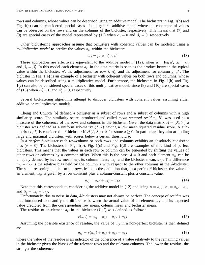
rows and columns, whose values can be described using an additive model. The biclusters in Fig. 1(b) andFig. 1(c) can be considered special cases of this general additive model where the coherence of valuescan be observed on the rows and on the columns of the bicluster, respectively. This means that (7) and(9) are special cases of the model represented by (12) whenαi = 0 andβj = 0, respectively.

Other biclustering approaches assume that biclusters with coherent values can be modeled using amultiplicative modelto predict the valuesaij within the bicluster:

aij = µ′ × α′i × β′j (13)

These approaches are effectively equivalent to the additive model in (12), whenµ = log µ′, αi = α′iandβj = β′j. In this model each elementaij in the data matrix is seen as the product between the typicalvalue within the bicluster,µ′, the adjustment for rowi, α′i, and the adjustment for columnj, β′j. Thebicluster in Fig. 1(e) is an example of a bicluster with coherent values on both rows and columns, whosevalues can be described using a multiplicative model. Furthermore, the biclusters in Fig. 1(b) and Fig.1(c) can also be considered special cases of this multiplicative model, since (8) and (10) are special casesof (13) whenα′i = 0 andβ′j = 0, respectively.

Several biclustering algorithms attempt to discover biclusters with coherent values assuming eitheradditive or multiplicative models.

Cheng and Church [6] defined a bicluster as a subset of rows and a subset of columns with a highsimilarity score. The similarity score introduced and calledmean squared residue, H, was used as ameasure of the coherence of the rows and columns in the bicluster. Given the data matrixA = (X,Y ) abicluster was defined as a uniform sub-matrix(I, J) having a low mean squared residue score. A sub-matrix (I, J) is considered aδ-bicluster if H(I, J) < δ for someδ ≥ 0. In particular, they aim at findinglarge and maximal biclusters with scores below a certain thresholdδ.

In a perfectδ-bicluster each row/column or both rows and columns exhibits an absolutely consistentbias (δ = 0). The biclusters in Fig. 1(b), Fig. 1(c) and Fig. 1(d) are examples of this kind of perfectbiclusters. This means that the values in each row or column can be generated by shifting the values ofother rows or columns by a common offset. When this is the case,δ = 0 and each elementaij can beuniquely defined by its row mean,aiJ , its column mean,aIj, and the bicluster mean,aIJ . The differenceaIj − aIJ is the relative bias held by the columnj with respect to the other columns in theδ-bicluster.The same reasoning applied to the rows leads to the definition that, in a perfectδ-bicluster, the value ofan element,aij, is given by a row-constant plus a column-constant plus a constant value:

aij = aiJ + aIj − aIJ (14)

Note that this corresponds to considering the additive model in (12) and usingµ = aIJ , αi = aiJ − aIJ

andβj = aIj − aIJ .Unfortunately, due to noise in data,δ-biclusters may not always be perfect. The concept ofresiduewas

thus introduced to quantify the difference between the actual value of an elementaij and its expectedvalue predicted from the corresponding row mean, column mean and bicluster mean.

The residue of an elementaij in the bicluster(I, J) was defined as follows:

r(aij) = aij − aiJ − aIj + aIJ (15)

Assuming the possible existence of residue, the value ofaij in a non-perfect bicluster is then definedas:

aij = r(aij) + aiJ + aIj − aIJ (16)

where the value of the residue is an indicator of the coherence of a value relatively to the remaining valuesin the bicluster given the biases of the relevant rows and the relevant columns. The lower the residue, thestronger the coherence.


In order to assess the overall quality of aδ-bicluster, Cheng and Church defined themean squaredresidue, H, of a bicluster(I, J) as the sum of the squared residues. The mean squared residue score isgiven by:

H(I, J) = 1|I||J |

∑i∈I,j∈J r(aij)

2 (17)

Using this merit function makes it possible to find biclusters with coherent values across both rows andcolumns since a scoreH(I, J) = 0 indicates that the values in the data matrix fluctuate in unison. Thisincludes, as a particular case, biclusters with constant values, which were addressed in Section III-B.

The mean squared residue score defined by Cheng and Church assumes there are no missing valuesin the data matrix. To guarantee this precondition, they replace the missing values by random numbers,during a preprocessing phase.

Yang et al. [29] [30] generalized the definition of aδ-bicluster to cope with missing values and avoidthe interference caused by the random fillins used by Cheng and Church. They defined aδ-bicluster as asubset of rows and a subset of columns exhibiting coherent values on the specified (non-missing) valuesof the rows and columns considered. The FLOC (FLexible Overlapped biClustering) algorithm introducedan occupancythreshold,ϑ, and defined aδ-bicluster ofϑ occupancy as a sub-matrix(I, J), where foreach rowi ∈ I, |J ′i |

|J | > ϑ, and for eachj ∈ J ,|I′j ||I| > ϑ. |J ′i | and |I ′j| are the number of specified elements

on row i and columnj, respectively. Thevolumeof the δ-bicluster,υIJ , was defined as the number ofspecified values ofaij. Note that the definition of Cheng and Church is a special case of this definitionwhenϑ = 1.

The termbasewas used to represent the bias of a row or column within aδ-bicluster(I, J). The baseof a row i, the base of a columnj and the base of theδ-bicluster (I, J) are the mean of all specifiedvalues in rowi, in columnj and in the bicluster(I, J), respectively. This allows us to redefineaiJ , aIj,aIJ andr(aij) andH(I, J), in (1), (2), (3) and (15), respectively, so that their calculus does not take intoaccount missing values:

aiJ = 1|J ′i |

∑j∈J ′i

aij (18)

aIj = 1|I′j |

∑i∈I′j

aij (19)

aIJ = 1υIJ

∑i∈I′i,j∈J ′j

aij (20)

r(aij) =

{aij − aiJ − aIj + aIJ , if aij is specified0 , otherwise

(21)

Yang et al. also considered that the coherence of a bicluster can be computed using the mean residueof all (specified) values. Moreover, they considered that this mean can be either arithmetic, geometric, orsquare mean. The arithmetic mean was used in [29]:

H(I, J) = 1υIJ

∑i∈I′j ,j∈J ′i

|r(aij)| (22)

The square mean was used in [30] and redefines Cheng and Church’s score, which was defined in (17),as follows:

H(I, J) = 1υIJ

∑i∈I′j ,j∈J ′i

r(aij)2 (23)

Wang el al. [28] also assumed the additive model in (12) and seek to discoverδ-pClusters. Given asub-matrix(I, J) of A, they consider each2 × 2 sub-matrixM = (Ii1i2 , Jj1j2) defined by each pair ofrows i1, i2 ∈ I and each pair of columnsj1, j2 ∈ J . The pscore(M)is computed as follows:

pscore(M) = |(ai1j1 − ai1j2)− (ai2j1 − ai2j2)| (24)


They consider that the sub-matrix(I, J) is a δ-pCluster if for any2 × 2 sub-matrixM ⊂ (I, J),pscore(M) < δ. They aim at findingδ-pClusters (pattern clusters), which are in fact biclusters withcoherent values. An example of a perfectδ-pCluster modeled using an additive model is the one presentedin Fig. 1(d). However, if the valuesaij in the data matrix are transformed usingaij = log(aij) this approachcan also identify biclusters defined by the multiplicative model in (13). An example of a perfectδ-pClustermodeled using a multiplicative model is the one presented in Fig. 1(e).

Kluger et al. [16] also addressed the problem of identifying biclusters with coherent values and lookedfor checkerboard structures in the data matrix by integrating biclustering of rows and columns withnormalization of the data matrix. They assumed that after a particular normalization, which was designedto accentuate biclusters if they exist, the contribution of a bicluster is given by a multiplicative modelas defined in (13). Moreover, they use gene expression data and see each valueaij in the data matrix asthe product of the background expression level of genei, the tendency of genei to be expressed in allconditions and the tendency of all genes to be expressed in conditionj. In order to access the qualityof a biclustering, Kluger et al. tested the results against a null hypothesis of no structure in the data matrix.

Tang et al. [25] introduced the Interrelated Two-Way Clustering (ITWC) algorithm that combines theresults of one-way clustering on both dimensions of the data matrix in order to produce biclusters. Afternormalizing the rows of the data matrix, they compute the vector-angle cosine value between each rowand a pre-defined stable pattern to test whether the row values vary much among the columns and removethe ones with little variation. After that they use a correlation coefficient as similarity measure to measurethe strength of the linear relationship between two rows or two columns, to perform two-way clustering.As this similarity measure depends only on the pattern and not on the absolute magnitude of the spatialvector, it also permits the identification of biclusters with coherent values represented by the multiplicativemodel in (13).

The previous biclustering approaches are based either on additive or multiplicative models, whichevaluate separately the contribution of each bicluster without taking into consideration the interactionsbetween biclusters. In particular, they do not explicitly take into account that the value of a given element,aij, in the data matrix can be seen as a sum of the contributions of the different biclusters to whom therow i and the columnj belong.

Lazzeroni and Owen [17] addressed this limitation by introducing the plaid model where the value ofan element in the data matrix is viewed as a sum of terms called layers. In the plaid model the data matrixis described as a linear function of variables (layers) corresponding to its biclusters.

The plaid model is defined as follows:

aij =∑K

k=0 θijkρikκjk (25)

where K is the number of layers (biclusters) and the value ofθijk specifies the contribution of eachbiclusterk specified byρik andκjk. The termsρik andκjk are binary values that represent, respectively,the membership of rowi and columnj in biclusterk.

Lazzeroni and Owen [17] want to obtain a plaid model, which describes the interactions between theseveral biclusters on the data matrix and minimizes the following merit function:

12

∑ni=1

∑mj=1 (aij − θij0 −∑K

k=1 θijkρikκjk)2

(26)

where the termθij0 considers the possible existence of a single bicluster that covers the whole matrix andthat explains away some variability that is not particular to any specific bicluster.

The plaid model described in (25) can be seen as a generalization of the additive model presented in(12). We will call this model thegeneral additive model. For every elementaij it represents a sum of


additive models each representing the contribution of the bicluster(I, J)k to the value ofaij in casei ∈ Iand j ∈ J .

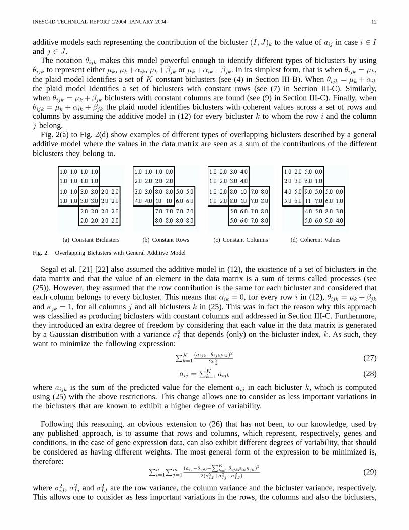
The notationθijk makes this model powerful enough to identify different types of biclusters by usingθijk to represent eitherµk, µk +αik, µk +βjk or µk +αik +βjk. In its simplest form, that is whenθijk = µk,the plaid model identifies a set ofK constant biclusters (see (4) in Section III-B). Whenθijk = µk + αik

the plaid model identifies a set of biclusters with constant rows (see (7) in Section III-C). Similarly,whenθijk = µk +βjk biclusters with constant columns are found (see (9) in Section III-C). Finally, whenθijk = µk + αik + βjk the plaid model identifies biclusters with coherent values across a set of rows andcolumns by assuming the additive model in (12) for every biclusterk to whom the rowi and the columnj belong.

Fig. 2(a) to Fig. 2(d) show examples of different types of overlapping biclusters described by a generaladditive model where the values in the data matrix are seen as a sum of the contributions of the differentbiclusters they belong to.

(a) Constant Biclusters (b) Constant Rows (c) Constant Columns (d) Coherent Values

Fig. 2. Overlapping Biclusters with General Additive Model

Segal et al. [21] [22] also assumed the additive model in (12), the existence of a set of biclusters in thedata matrix and that the value of an element in the data matrix is a sum of terms called processes (see(25)). However, they assumed that the row contribution is the same for each bicluster and considered thateach column belongs to every bicluster. This means thatαik = 0, for every rowi in (12), θijk = µk + βjk

andκjk = 1, for all columnsj and all biclustersk in (25). This was in fact the reason why this approachwas classified as producing biclusters with constant columns and addressed in Section III-C. Furthermore,they introduced an extra degree of freedom by considering that each value in the data matrix is generatedby a Gaussian distribution with a varianceσ2

k that depends (only) on the bicluster index,k. As such, theywant to minimize the following expression:

∑Kk=1

(aijk−θijkρik)2

2σ2k

(27)

aij =∑K

k=1 aijk (28)

whereaijk is the sum of the predicted value for the elementaij in each biclusterk, which is computedusing (25) with the above restrictions. This change allows one to consider as less important variations inthe biclusters that are known to exhibit a higher degree of variability.

Following this reasoning, an obvious extension to (26) that has not been, to our knowledge, used byany published approach, is to assume that rows and columns, which represent, respectively, genes andconditions, in the case of gene expression data, can also exhibit different degrees of variability, that shouldbe considered as having different weights. The most general form of the expression to be minimized is,therefore: ∑n

i=1

∑mj=1

(aij−θij0−∑K

k=1θijkρikκjk)2

2(σ2iJ+σ2

Ij+σ2IJ )

(29)

whereσ2iJ , σ2

Ij andσ2IJ are the row variance, the column variance and the bicluster variance, respectively.

This allows one to consider as less important variations in the rows, the columns and also the biclusters,


that are know to exhibit a higher degree of variability.

Other possibility that has not been, to our knowledge, used by any published approach, is to considerthat the value of a given element,aij, in the data matrix is given by the product of the contributions ofthe different biclusters to whom the rowi and the columnj belong, instead of a sum of contributions asit is considered by the plaid model. In this approach, which we will callgeneral multiplicative model, thevalue of each elementaij in the data matrix is given by the following expression:

aij =∏K

k=0 θijkρikκjk (30)

Similarly to the plaid model that sees a bicluster as a sum of layers (biclusters), (30) describes the valueaij in the data matrix as a product of layers. The notationθijk is now used to represent eitherµk, µk×αik,µk×βjk or µk×αik×βjk. Hence, in its general case,θijk is now given by the multiplicative model in (13)instead of being defined by the additive model in (12), as the plaid model was. Fig. 3(a) to Fig. 3(d) showexamples of different types of overlapping biclusters described by a general multiplicative model where thevalues in the data matrix are seen as a product of the contributions of the different biclusters they belong to.

Conceptually, it is also possible to combine the general multiplicative model in (30) withθijk given bythe additive model in (12). Such a combination would consider an additive model for each bicluster, but amultiplicative model for the combination of the contributions given by the several biclusters. Similarly, itis also possible to combine the general additive model in (25) withθijk given by the multiplicative modelin (13). This corresponds to considering that each bicluster is generated using a multiplicative model,but the combination of biclusters is performed using an additive model. These combinations, however,are less likely to be useful than the general additive model ((12) and (25)) and the general multiplicativemodel ((13) and (30)).

(a) Constant Biclusters (b) Constant Rows (c) Constant Columns (d) Coherent Values

Fig. 3. Overlapping Biclusters with General Multiplicative Model

The previous biclustering algorithms used either an additive or multiplicative model to produce biclusterswith coherent values and can for this reason be put in the same framework. In these bicluster models, abackground value is used together with the row and column effects to predict the values within the biclusterand find bicluster that satisfy a certain coherence criterion regarding their values. The last approaches weanalyzed consider that the value of a given element in the data matrix can be seen as a sum of thecontributions of the different biclusters to whom its rows and columns belong, while the other considerthe contribution of a bicluster at a time. We also looked at the possibility to consider the values in the datamatrix as a product of the contributions of several biclusters. Nevertheless, all the previously surveyedbiclustering algorithms try to discover sets of biclusters by analyzing directly the valuesaij in the datamatrix A.

E. Biclusters with Coherent Evolutions

In the previous section we revised several biclustering algorithms that aimed at discovering biclusterswith coherent values. Other biclustering algorithms address the problem of finding coherent evolutions


across the rows and/or columns of the data matrix regardless of their exact values. In the case of geneexpression data, we may be interested in looking for evidence that a subset of genes is up-regulated ordown-regulated across a subset of conditions without taking into account their actual expression values inthe data matrix. The co-evolution property can be observed on both rows and columns of the biclusters,as it is shown in Fig. 1(f), on the rows of the bicluster or on its columns. The biclusters presented in Fig.1(h) and Fig. 1(i) are examples of biclusters with coherent evolutions on the columns, while Fig. 1(g)shows a bicluster with co-evolution on the rows.

Ben-Dor et al. [2] defined a bicluster as an order-preserving sub-matrix (OPSM). According to theirdefinition, a bicluster is a group of rows whose values induce a linear order across a subset of the columns.Their work focus on the relative order of the columns in the bicluster rather than on the uniformity ofthe actual values in the data matrix as the plaid model [17] did. More specifically, they want to identifylarge OPSMs. A sub-matrix is order-preserving if there is a permutation of its columns under which thesequence of values in every row is strictly increasing. The bicluster presented in Fig. 1(i) is an example ofan OPSM, whereai4 ≤ ai2 ≤ ai3 ≤ ai1, and represents a bicluster with coherent evolution on its columns.Furthermore, Ben-Dor et al. defined a complete model as the pair(J, π), where J is a set ofs columnsandπ = (j1, j2, ..., js) is a linear ordering of the columns inJ . They say that a row supports(J, π) if thes corresponding values, ordered according to the permutationπ are monotonically increasing.

Although the straightforward approach to the OPSM problem would be to find a maximum supportcomplete model, that is, a set of columns with a linear order supported by a maximum number ofrows, Ben-Dor et al. aimed at finding a complete model with highest statistically significant support. Thestatistical significance of a given OPSM is thus computed using an upper-bound on the probability thata random data matrix of sizen-by-m will contain a complete model of sizes with k or more rowssupporting it. In the case of gene expression data such a sub-matrix is determined by a subset of genesand a subset of conditions, such that, within the set of conditions, the expression levels of all genes havethe same linear ordering. As such, Ben-Dor et al. addressed the identification and statistical assessmentof co-expressed patterns for large sets of genes. They also considered that, in many cases, data containsmore than one such pattern.

Following the same idea, Liu and Wang [18] defined a bicluster as an OP-Cluster (Order PreservingCluster). Their goal is also to discover biclusters with coherent evolutions on the columns. Hence, thebicluster presented in Fig. 1(i) is an example of an OPSM and also of an OP-Cluster.

Murali and Kasif [19] aimed at finding conserved gene expression motifs (xMOTIFs). They defined anxMOTIF as a subset of genes (rows) that is simultaneously conserved across a subset of the conditions(columns). The expression level of a gene is conserved across a subset of conditions if the gene is inthe same state in each of the conditions in this subset. They consider that a gene state is a range ofexpression values and assume that there are a fixed given, number of states. These states can simply beup-regulated and down-regulated, when only two states are considered. An example of a perfect biclusterin this approach is the one presented in Fig. 1(g), whereSi is the symbol representing the preserved stateof the row (gene)i.

Murali and Kasif assumed that data may contain several xMOTIFs (biclusters) and aimed at finding thelargest xMOTIF: the bicluster that contains the maximum number of conserved rows. The merit functionused to evaluated the quality of a given bicluster is thus the size of the subset of rows that belong to it.Together with this conservation condition, an xMOTIF must also satisfy size and maximality properties:the number of columns must be in at least anα-fraction of all the columns in the data matrix, and forevery row not belonging to the xMOTIF the row must be conserved only in aβ-fraction of the columns init. Note that this approach is similar to the one followed by Ben-Dor et al. [2]. Ben-Dor et al. consideredthat rows (genes) have only two states (up-regulated and down-regulated) and looked for a group of rowswhose states induce some linear order across a subset of the columns (conditions). This means that the


expression level of the genes in the bicluster increased or decreased from condition to condition. Muraliand Kasif [19] consider that rows (genes) can have a given number of states and look for a group ofcolumns (conditions) within which a subset of the rows is in the same state.

Tanay et al. [24] defined a bicluster as a subset of genes (rows) that jointly respond across a subset ofconditions (columns). A gene is considered to respond to a certain condition if its expression level changessignificantly at that condition with respect to its normal level. Before SAMBA (Statistical-AlgorithmicMethod for Bicluster Analysis) is applied, the expression data matrix is modeled as a bipartite graphwhose two parts correspond to conditions (columns) and genes (rows), respectively, with one edge foreach significant expression change. SAMBA’s goal is to discover biclusters (sub-graphs) with an overallcoherent evolution. In order to do that it is assumed that all the genes in a given bicluster are up-regulatedin the subset of conditions that form the bicluster and the goal is then to find the largest biclusters withthis co-evolution property. As such, SAMBA does not try to find any kind of coherence on the values,aij,in the bicluster. It assumes that regardless of its true value,aij is either 0 or 1, where1 is up-regulationand 0 is down-regulation. A large bicluster is thus one with a maximum number of genes (rows) whosevalue aij is expected to be 1 (up-regulation). The bicluster presented in Fig. 1(f) is an example of thetype of bicluster SAMBA produces, if we say thatS1 is the symbol that represents a coherent overallup-regulation evolution. The merit function used to evaluate the quality of a computed bicluster usingSAMBA is the weight of the sub-graph that models it. Its statistical significance is evaluated by computingthe probability of finding at random a bicluster with at least its weight. Given that the weight of a sub-graph is defined as the sum of the weights of gene-condition (row-column) pairs in it including edges andnon-edges, the goal is thus to assign weights to the vertex pairs of the bipartite sub-graph so that heavysub-graphs correspond to significant biclusters.

IV. B ICLUSTER STRUCTURE

Biclustering algorithms assume one of the following situations: either there is onlyone biclusterin thedata matrix (see Fig. 4(a)), or the data matrix containsK biclusters, whereK is the number of biclusterswe expect to identify and is usually definedapriori. While most algorithms assume the existence ofseveral biclusters in the data matrix [13] [6] [11] [5] [17] [21] [25] [29] [4] [24] [30] [16] [23] [22] [18],others only aim at finding one bicluster. In fact, even though these algorithms can possibly find more thanone bicluster, the target bicluster is usually the one considered the best according to some criterion [2] [19].

When the biclustering algorithm assumes the existence of several biclusters in the data matrix, thefollowing bicluster structures can be obtained (see Fig. 4(b) to Fig. 4(i)):

1) Exclusive row and column biclusters (rectangular diagonal blocks after row and column reorder).2) Non-Overlapping biclusters with checkerboard structure.3) Exclusive-rows biclusters.4) Exclusive-columns biclusters.5) Non-Overlapping biclusters with tree structure.6) Non-Overlapping non-exclusive biclusters.7) Overlapping biclusters with hierarchical structure.8) Arbitrarily positioned overlapping biclusters.

A natural starting point to achieve the goal of identifying several biclusters in a data matrixA is to forma color image of it with each element colored according to the value ofaij. It is natural then to considerways of reordering the rows and columns in order to group together similar rows and similar columns,thus forming an image with blocks of similar colors. These blocks are subsets of rows and subsets ofcolumns with similar expression values, hence, biclusters. An ideal reordering of the data matrix wouldproduce an image with some numberK of rectangular blocks on the diagonal (see Fig. 4(b)). Each block


(a) Single Bicluster (b) Exclusive row andcolumn biclusters

(c) Checkerboard Struc-ture

(d) Exclusive-rowsbiclusters

(e) Exclusive-columnsbiclusters

(f) Non-Overlapping bi-clusters with tree struc-ture

(g) Non-Overlappingnon-exclusive biclusters

(h) Overlappingbiclusters withhierarchical structure

(i) Arbitrarily positionedoverlapping biclusters

Fig. 4. Bicluster Structure

would be nearly uniformly colored, and the part of the image outside of these diagonal blocks wouldbe of a neutral background color. This ideal corresponds to the existence ofK mutually exclusive andexhaustive clusters of rows, and a correspondingK-way partitioning of the columns, that is,K exclusiverow and column biclusters. In this biclustering structure, every row in the row-blockk is expressed within,and only within, those columns in condition-blockk. That is, every row and every column in the datamatrix belongs exclusively to one of theK biclusters considered (see Fig. 4(b)). Although this can be thefirst approach to extract relevant knowledge from gene expression data, it has long been recognized thatsuch an ideal reordering, which would lead to such a bicluster structure, will seldom exist in real data[17].

Facing this fact, the next natural step is to consider that rows and columns may belong to more thanone bicluster, and assume a checkerboard structure in the data matrix (see Fig. 4(c)). By doing this weallow the existence ofK non-overlapping and non-exclusive biclusters where each row in the data matrixbelongs to exactlyK biclusters. The same applies to columns. Kluger et al. [16] assumed this structureon cancer data. The Double Conjugated Clustering (DCC) approach introduced by Busygin et al. [4] alsomakes it possible to identify this biclustering structure. However, DCC tends to produce the structure inFig. 4(b).

Other biclustering approaches assume that rows can only belong to one bicluster, while columns, whichcorrespond to conditions in the case of gene expression data, can belong to several biclusters. Thisstructure, which is presented in Fig. 4(d), assumes exclusive-rows biclusters and was used by Sheng etal. [23] and Tang et al. [25]. However, these approaches can also produce exclusive-columns biclusterswhen the algorithm is used using the opposite orientation of the data matrix. This means that the columnsof the data matrix can only belong to one bicluster while the rows can belong to one or more biclusters(see Fig. 4(e)).

The structures presented in Fig. 4(b) to Fig. 4(e) assume that the biclusters are exhaustive, that is, everyrow and every column in the data matrix belongs at least to one bicluster. However, we can considernon-exhaustive variations of these structures that make it possible that some rows and columns do notbelong to any bicluster. Other exhaustive bicluster structures, include the tree structure considered byHartigan [13] and Tibshirani et al. [26] and that is depicted in Fig. 4(f), and the structure in Fig. 4(g). Anon-exhaustive variation of the structure presented in Fig. 4(g) was assumed by Wang et al. [28]. Noneof these structures allow overlapping, that is, none of these structures makes it possible that a particular


pair (row,column) belongs to more than one bicluster.

The previous bicluster structures are restrictive in many ways. On one hand, some of them assumethat, for visualization purposes, all the identified biclusters should be observed directly on the data matrixand displayed as a contiguous representation after performing a common reordering of their rows andcolumns. On the other hand, others assume that the biclusters are exhaustive that is, every row and everycolumn in the data matrix belongs to at least one bicluster. However, it is more likely that, in real data,some rows or columns do not belong to any bicluster at all and that the biclusters overlap in some places.It is, however possible to enable these two properties without relaxing the visualization property if thehierarchical structure proposed by Hartigan is assumed. This structure, depicted in Fig. 4(h), requires thateither the biclusters are disjoint or one includes the other. Two specializations of this structure, are the treestructure presented in Fig. 4(f), where the biclusters form a tree, and the checkerboard structure depictedin Fig. 4(c), where the biclusters, the row clusters and the column clusters are all trees.

A more general bicluster structure permits the existence ofK possibly overlapping biclusters withouttaking into account their direct observation in the data matrix with a common reordering of its rows andcolumns. Furthermore, these non-exclusive biclusters can also be non-exhaustive, which means that somerows or columns may not belong to any bicluster. Several biclustering algorithms [6] [17] [11] [5] [25][21] [24] [2] [19] [22] [18] allow this more general structure, which is presented in Fig. 4(i).

The plaid model [17], defined in (25), can be used to describe most of these different biclustersstructures. The restriction that every row and every column are in exactly one bicluster correspond tothe conditions

∑k ρik = 1, for all i, and

∑k κjk = 1 for all j. To allow overlapping it is necessary that∑

k ρik ≥ 2, for somei, and∑

k κjk ≥ 2, for somej. Similarly, allowing that some rows or columns donot belong to any bicluster corresponds to the restrictions

∑k ρik = 0, for somei, and

∑k κjk = 0, for

somej. This means that without any of these constrains, the plaid model represents the data matrix as asum of possibly overlapping biclusters as presented in Fig. 4(i).

V. A LGORITHMS

Biclustering algorithms may have two different objectives: to identify one or to identify a given numberof biclusters. Some approaches attempt to identifyone bicluster at a time. Cheng and Church [6] andSheng et al. [23], for instance, identify a bicluster at a time, mask it with random numbers, and repeat theprocedure in order to eventually find other biclusters. Lazzeroni and Owen [17] also attempt to discoverone bicluster at a time in an iterative process where a plaid model is obtained. Ben-Dor et al. [2] alsoidentify one bicluster at a time.

Other biclustering approaches discoverone set of biclusters at a time. Hartigan [13] identifies twobiclusters at the time by splicing each existing bicluster into two pieces at each iteration. CTWC [11]performs two-way clustering on the row and column dimensions of the data matrix separately. It uses ahierarchical clustering algorithm that generates stable clusters of rows and columns, at each iteration, andconsequently discovers a set of biclusters at a time. A similar procedure is followed by ITWC [25].

We also analyzed algorithms that performsimultaneous bicluster identification, which means that thebiclusters are discovered all at the same time. FLOC [29], [30] follows this approach. It first generates a setof initial biclusters by adding each row/column to each one of them with independent probability and theniteratively improves the quality of the biclusters. Muraly and Kasif [19] also identify several xMOTIFs(biclusters) simultaneously, although they only report the one that is considered the best according tothe size and maximality criteria used. Tanay et al. [24] use SAMBA to performs simultaneous biclusteridentification using exhaustive bicluster enumeration, but restricting the number of rows the biclustersmay have. Liu and Yand [18] and Yang et al. [28] also used exhaustive bicluster enumeration to performsimultaneous biclustering identification. The approaches followed by Busygin et al. [4], Kluget et al. [16]and Califano et al. [5] also discover all the biclusters at the same time.


Given the complexity of the problem, a number of different heuristic approaches has been used toaddress this problem. They can be divided into five classes, studied in the following five subsections:

1) Iterative Row and Column Clustering Combination.2) Divide and Conquer.3) Greedy Iterative Search.4) Exhaustive Bicluster Enumeration.5) Distribution Parameter Identification.

The straightforward way to perform bicluster identification is to apply clustering algorithms to the rowsand columns of the data matrix, separately, and then to combine the results using some sort of iterativeprocedure to combine the two cluster arrangements. Several algorithms use thisiterative row and columnclustering combinationidea, and are described in Section V-A.

Other approaches use adivide-and-conquerapproach: they break the problem into several subproblemsthat are similar to the original problem but smaller in size, solve the problems recursively, and thencombine these solutions to create a solution to the original problem [7]. These biclustering approachesare described in Section V-B.

A large number of methods, studied in section V-C, perform some form ofgreedy iterative search. Theyalways make a locally optimal choice in the hope that this choice will lead to a globally good solution[7].

Some authors propose methods that performexhaustive bicluster enumeration. A number of methodshave been used to speed up exhaustive search, in some cases assuming restrictions on the size of thebiclusters that should be listed. These algorithms are revised in Section V-D.

The last type of approach we identified performsdistribution parameter identification. These approachesassume that the biclusters are generated using a given statistical model and try to identify the distributionparameters that fit, in the best way, the available data, by minimizing a certain criterion through an iterativeapproach. Section V-E describes these approaches.

A. Iterative Row and Column Clustering Combination

The conceptually simpler way to perform biclustering using existing techniques is to apply standardclustering methods on the column and row dimensions of the data matrix, and then combine the resultsto obtain biclusters. A number of authors have proposed methods based on this idea.

The Coupled Two-Way Clustering (CTWC) [11] seeks to identify couples of relatively small subsetsof features (Fi) and objects (Oj), where bothFi andOj can be either rows or columns, such that whenonly the features inFi are used to cluster the corresponding objectsOj, stable and significant partitionsemerge. It uses a heuristic to avoid brute-force enumeration of all possible combinations: only subsets ofrows or columns that are identified as stable clusters in previous clustering iterations are candidates forthe next iteration.

CTWC begins with only one pair of rows and columns, where each pair is the set containing all rowsand the set that contains all columns, respectively. A hierarchical clustering algorithm is applied on eachset generating stable clusters of rows and columns, and consequently a set of biclusters at a time. Atunable parameterT controls the resolution of the performed clustering. The clustering starts atT = 0with a single cluster that contains all the rows and columns. AsT increases, phase transitions take place,and this cluster breaks into several sub-clusters. Clusters keep breaking up asT is further increased, untilat high enough values ofT each row and column forms its own cluster. The control parameterT is usedto provide a measure for the stability of any particular cluster by the range of values∆T at which thecluster remains unchanged. A stable cluster is expected to survive throughout a large∆T , one whichconstitutes a significant fraction of the range it takes the data to break into single point clusters.


During its execution, CTWC dynamically maintains two lists of stable clusters (one for row clusters andone for column clusters) and a list of pairs of row and column subsets. At each iteration, one row subsetand one column subset are coupled and clustered mutually as objects and features. Newly generated stableclusters are added to the row and column lists and a pointer that identifies the parent pair is recordedto indicate where this cluster came from. The iteration continues until no new clusters that satisfy somecriteria such as stability and critical size are found.

The Interrelated Two-Way Clustering (ITWC) [25] is an iterative biclustering algorithm based on acombination of the results obtained by clustering performed on each of the two dimensions of the datamatrix separately. Within each iteration of ITWC there are five main steps.

In the first step, clustering is performed in the row dimension of the data matrix. The task in this stepis to clustern1 rows into K groups, denoted asIi, i = 1, ..., K, each of which is an exclusive subsetof the set of all rowsX. The clustering technique used can be any method that receives the number ofclusters. Tang et al. used K-means. In the second step, clustering is performed in the column dimensionof the data matrix. Based on each groupIi, i = 1, ..., k, the columns are independently clustered into twoclusters, represented byJi,a andJi,b.

Assume, for simplicity, that the rows have been clustered into two groups,I1 and I2. The third stepcombines the clustering results from the previous steps by dividing the columns into four groups,Ci,i = 1, ..., 4, that correspond to the possible combinations of the column clustersJ1,x andJ2,x, x = {a, b}.

The fourth step of ITWC aims at finding heterogeneous pairs(Cs, Ct), s, t = 1, ..., 4. Heterogeneouspair are groups of columns that do not share row attributes used for clustering. The result of this step isa set of highly disjoint biclusters, defined by the set of columns inCs andCt and the rows used to definethe corresponding clusters. Finally, ITWC sorts the rows of the matrix in descending order of the cosinedistance between each row and a row representative of each bicluster (obtained by considering the value1 in each entry for columns inCs and Ct, respectively). The first one third of rows is kept. By doingthis they obtain a reduced row sequenceI ′ for each heterogeneous group. In order to select the row setI ′ that should be chosen for the next iteration of the algorithm they use cross-validation. After this finalstep the number of rows are reduced fromn1 to n2 and the above five steps can be repeated using then2 selected rows until the termination conditions of the algorithm are satisfied.

The Double Conjugated Clustering (DCC) [4] performs clustering in the rows and columns dimen-sions/spaces of the data matrix using self-organizing maps (SOM) and the angle-metric as similaritymeasure. The algorithm starts by assigning every node in one space, (either a row or a column) to aparticular node of the second space, which is called conjugated node. The clustering is then performedin two spaces. The first one is called the feature space, havingn dimensions representing the rows of thedata matrix. In the second space, called the sample space, the roles of the features and samples have beenexchanged. This space hasm dimensions, corresponding to the columns of the data matrix, and is usedto perform clustering on then features which are now the rows of the data matrix.

To convert a node of one space to the other space, DCC makes use of the angle between the node andeach of the patterns. More precisely, theith conjugate entry is the dot product between the node vectorand theith pattern vector of the projected space when both the vectors are normalized to unit length.Formally, they introduce the matricesX1 andX2, which corresponds to the original data matrixX afterits columns and rows have been, respectively, normalized to unit length. The synchronization betweenfeature and sample spaces is forced by alternating clustering in both spaces. The projected clusteringresults of one space are used to correct the positions of the corresponding nodes of the other space. Ifthe node update steps are small enough, both processes will converge to a state defined by a compromisebetween the two clusterings. Since the feature and sample spaces maximize sample and feature similarity,respectively, such a solution is desirable.

DCC works iteratively by performing a clustering cycle and then transforming each node to the conjugatespace where the next training cycle takes place. This process is repeated until the number of moved


samples/features falls below a certain threshold in both spaces. DCC returns two results: one in featurespace and one in sample space, each being the conjugate of the other. Since every sample cluster in thefeature space corresponds to a feature in the sample space, DCC derives a group of rows for every groupof columns, hence, a set of biclusters.

B. Divide-and-Conquer

Divide and conquer algorithms have the significant advantage of being potentially very fast. However,they have the very significant drawback of being likely to miss good biclusters that may be split beforethey can be identified.

Block clustering was the first divide-and-conquer approach to perform biclustering. Block clusteringis a top down, row and column clustering of the data matrix. The basic algorithm for forward blocksplitting was due to Hartigan [13] who called it direct clustering (see Section III-B). The block clusteringalgorithm begins with the entire data in one block (bicluster). At each iteration it finds the row or columnthat produces the largest reduction in the total “within block” variance by splicing a given block intotwo pieces. In order to find the best split into two groups the rows and columns of the data matrix aresorted by row and column mean, respectively. The splitting continues until a given numberK of blocksis obtained or the overall variance within the blocks reaches a certain threshold.

Since the estimation of the optimal number of splicings is difficult, Duffy and Quiroz [10] suggested theuse of permutation tests to determine when a given block split is not significant. Following this direction,Tibshirani et al. [26] added a backward pruning method to the block splitting algorithm introduced byHartigan [13] and designed a permutation-based method to induce the optimal number of biclusters,K,called Gap Statistics. In their approach the splitting continues until a large number of blocks are obtained.Some blocks are then recombined until the optimal number of blocks is reached. This approach is similarto the one followed in decision tree algorithms, where the tree is grown until a given depth and a pruningcriterion is used at the end.

C. Greedy Iterative Search

Greedy iterative search methods are based on the idea of creating biclusters by adding or removingrows/columns from them, using a criterion that maximizes thelocal gain. They may make wrong decisionsand loose good biclusters, but they have the potential to be very fast.

Cheng and Church [6] were the first to apply biclustering to gene expression data. Given a data matrixA and a maximum acceptable mean squared residue score (see (17)),δ > 0, the goal is to findδ-biclusters,that is, subsets of rows and subsets of columns,(I, J), with a score no larger thanδ (see Section III-D).In order to achieve this goal, Cheng and Church proposed several greedy row/column removal/additionalgorithms that are then combined in an overall approach that makes it possible to find a given numberK of δ-biclusters. The single node deletion method iteratively removes the row or column that gives themaximum decrease ofH. The multiple node deletion method follows the same idea. However, in eachiteration, it deletes all rows and columns with row/column residue superior to a given threshold. Finally,the node addition method adds rows and columns that do not increase the actual score of the bicluster.

In order to find a given number,K, of biclusters, greedy node deletion is performed first and is thenfollowed by greedy node addition. The algorithm discovers one bicluster at a time. At each of theKiterations, the algorithms starts with an initial bicluster that contains all rows and columns. This meansthat the algorithm starts with the entire matrixA and stops when no action decreasesH or whenH < δ.The discovered bicluster is then reported, and masked with random numbers, so that no recognizablestructures remain. The process is repeated untilK biclusters are found. Although masking previouslygenerated biclusters might suggest that it is not possible to find overlapping biclusters, this is in factpossible, since the node addition step is performed using the original values in the data matrix and not


the random ones introduced during the masking process. However, the discovery of highly overlappingbiclusters is not likely, since elements of already identified biclusters have been masked by random noise.

The FLOC (FLexible Overlapped biClustering) algorithm [29], [30] addresses this limitation (see SectionIII-D). It is based on the bicluster definition used by Cheng and Church but performs simultaneous biclusteridentification. It is also robust agains missing values, which are handled by taking into account the biclustervolume (number of non-missing elements) when computing the score (see (23)). This means that missingvalues are not used when computing the row mean, the column mean and the bicluster mean needed tocompute the score (see (18), (19) and (20)). FLOC avoids the introduction of random interference anddiscoversK possibly overlapping biclusters simultaneously.

FLOC has two phases. In the first phase,K initial biclusters are generated by adding each row/columnto each one of them with independent probabilityp. The second phase is an iterative process that improvesthe quality of these biclusters. During each iteration, each row and each column is examined to determinethe best action that can be taken towards reducing the overall mean score residue. An action is uniquelydefined at any stage with respect to a row/column and a bicluster. It represents the change of membershipof a row/column with respect to a specific bicluster: a row/column can be added to the bicluster, if it isnot yet included in it, or it can be removed if it already belongs to it. Since there areK biclusters, thereare K potential actions for each row/column. Among theseK actions, the one that has the maximumgain is identified and executed. The gain of an action is defined as a function of the relative reductionof the bicluster residue and the relative enlargement of the bicluster volume. At each iteration, the set ofselected actions is performed according to a random weighted order that assigns higher probabilities ofexecution to the actions with higher gains. The optimization process stops when the potential actions donot improve the overall quality of the biclustering.

Ben-Dor et al. [2] addressed the identification of large order-preserving submatrices (OPSMs) withmaximum statistical significance (see Section III-E). In order to do that they assume a probabilistic modelof the data matrix where there is a bicluster(I, J) determined by a set of rowsI, a set of columnsJ anda linear ordering of the columns inJ . Within each row of(I, J) the order of the elements is consistentwith the linear ordering ofJ . They define a complete model as the pair(J, π) where J is a set ofscolumns andπ = (j1, j2, ..., js) is a linear ordering of the columns inJ . A row supports(J, π) if the scorresponding values, ordered according to the permutationπ, are monotonically increasing.

Since an exhaustive algorithm that tries all possible complete models is not feasible, the idea is to growpartial models iteratively until they become complete models. A partial model of order(a, b) specifies, inorder, the indices of thea “smallest” elements< j1, ..., ja > and the indices of theb “largest” elements< js−(b−1), ..., js > of a complete model(J, π) and its sizes.

The OPSM algorithm focus on the columns at the extremes of the ordering when defining partialmodels, assuming that these columns are more useful in identifying the target rows, that is, the rows thatsupport the assumed linear order. The algorithm starts by evaluating all(1, 1) partial models and keepingthe bestl of them. It then expands them to(2, 1) models and keeps the bestl of them. After that itexpands them to(2, 2) models,(3, 2) models and so on until it getsl ([s/2], [s/2]) models, which arecomplete models. It then outputs the best one.

Murali and Kasif [19] introduced a biclustering algorithm that aims at finding xMOTIFs. An xMOTIFis a bicluster with coherent evolutions on its rows (see Section III-E). The data is discretized to a set ofsymbols by using a list of statistical significant intervals, for each row (gene, in the case of expressiondata), representing the states in which the gene is expressed within the set of conditions (columns).

To determine an xMOTIF it is necessary to compute the set of conserved rows,I, the states that theserows are in, and the set of columns,J , that match the motif. Given the set of conserved rows,I, the statesof the conserved rows, and one columnc that matches a given motif, it is easy to compute the remainingconditions inJ simply by checking, for each columnc′, if the rows inI are in the same state inc and


c′. Columnc is called a“seed” from which the entire motif can be computed. If one knows a conditionc that matches the largest xMOTIF in the data matrix, the goal of the algorithm is thus to compute therows that belong to this largest xMOTIF and the states they are in.

In order to pursue the goal of finding the largest xMOTIF, Murali and Kasif define adiscriminating setas a set of conditions,D, with the following two properties: (i) for every columnc′ in D and for everyrow in the largest motif, there is one state such that the row is in that state in columnsc andc′; and (ii)for every rowr that is not in the largest motif, there exists a columnc′ in D such that rowr is not in thesame state in columnsc and c′. The key property of a discriminating set is that given the seed columnc and such a setD, it is possible to compute the largest xMOTIF by including exactly those row-statesthat satisfy these properties and exactly those columns that agree withc on all these row-states.

The xMOTIF algorithm works by assuming that, for each row, there are a set of intervals correspondingto gene states, which are computed in the first step of the algorithm. This corresponds to a step ofdiscretization of the continuous data to a set of discrete symbols. The algorithm then proceeds by selectingns columns uniformly at random from the set of all columns. These columns act as seeds. Having done this,for each previously selected seed,c, the algorithm selectsnd sets of columns uniformly at random fromthe set of all columns. These sets havesd elements each and serve as candidates for the discriminating set,D. For each pair (seed, discriminating set) the corresponding xMOTIF is computed as explained above.The computed motif is discarded if less than anα-fraction of the columns match it. After all the seedshave been used to produce xMOTIFs, the largest xMOTIF, that is, the one that contains the largest numberof rows, is returned.

Califano et al. [5] introduced an algorithm that addresses the problem of findingδ-valid ks-patterns(see Section III-D). Their goal is to find groups of rows that exhibit coherent values in a subset of thecolumns but do not have any coherence of values in any of the remaining columns. After preprocessing thedata, they use a pattern discovery algorithm to discover sets of rows and columns candidate to becomestatistically significant biclusters (other candidates generated by the pattern discovery are discarded).Finally, an optimal set of patterns is chosen among the statistically significant ones using a greedy setcovering algorithm that adds rows and columns to the existing patterns so that they become maximalpatterns (see Section III-D).

The pattern discovery algorithm used considers that each column of the data matrix is a string anddiscovers patterns in these strings by allowing all possible string alignments. A density constraint is usedto limit the impact of random matches occurring over large distances on the strings and the strings arepre-aligned before the algorithm is used. The algorithm starts with a single pattern with no rows, allthe columns, and an offset of zero for each column. The values in each column are then sorted andall subsets of continuous values that areδ-valid (see Section III-D) are selected. Non-maximal subsetsthat are completely contained within another subset are removed. Each subset is considered a potentialsuper-patterns of a maximal pattern. All possible maximal combinations of these super-pattern are thencreated iteratively. As a result, all patterns that exists in the data matrix are generated hierarchically bypattern combination.

D. Exhaustive Bicluster Enumeration

Exhaustive bicluster enumeration methods are based on the idea that the best biclusters can only beidentified using an exhaustive enumeration of all possible biclusters existent in the data matrix. Thesealgorithms certainly find the best biclusters, if they exist, but have a very serious drawback. Due to theirhigh complexity, they can only be executed by assuming restrictions on the size of the biclusters.

Tanay et al. [24] introduced SAMBA (Statistical-Algorithmic Method for Bicluster Analysis), a bi-clustering algorithm that performs simultaneous bicluster identification by using exhaustive enumeration.SAMBA avoids an exponential runtime by restricting the number of rows the biclusters may exhibit. They


use the graph formalism described in Section II-A, and define as their objective the identification of amaximum weight sub-graph, assuming that the weight of a sub-graph will correspond to its statisticalsignificance.

Discovering the most significant biclusters in the data matrix under this weighting schemes is equivalentto the selection of the heaviest sub-graphs in the model bipartite graph. SAMBA assumes that row verticeshaved-bounded degree. This corresponds to a restriction on the size of the discovered biclusters since thenumber of rows cannot exceed this value. In the case of gene expression data this restriction is justifiedby the fact that genes that very frequently exhibit high expression levels are generally not interesting.

The first phase of the SAMBA algorithm normalizes the data, defining a gene as up-regulated or down-regulated if its standardized expression level (with mean0 and variance1), is, respectively, above 1 orbelow -1. In the second phase the algorithm finds theK heaviest bicliques in the graph. This is doneby looking at a pre-computed table with the weights of the bicliques intersecting every given column(condition) or row (gene) and choosing theK best bicliques. In order to improve the performance ofthis procedure, rows (genes) with degree exceedingd are ignored and the hashing for each row (gene)is performed only on subsets of its neighbors whose size is in a given range. In a postprocessing phase,SAMBA performs greedy addition or removal of vertices to perform a local improvement on the biclustersand filter the similar ones. Two biclusters are considered similar if their vertex sets (subset of rows andsubset of columns), differ only slightly. The intersection between two biclusters is defined as the numberof shared columns times the number of shared rows.

Wang et al. [28] also proposed an algorithm that performs exhaustive bicluster enumeration, subjectto a restriction that they should posses a minimum number of rows and a minimum number of columns.To speed up the process and avoid the repetition of computations, they use a suffix tree to efficientlyenumerate the possible combinations of row and column sets that represent valid biclusters.

The algorithm starts by deriving a set of candidateMaximum Dimension Sets(MDS) for each pair ofrows and for each pair of columns. An(x, y) row-pair MDS is a set of columns that defines a maximumwidth bicluster that includes rowsx and y. A similar definition holds for a column-pair MDS. The setof candidate MDS is computed using an efficient method that generates all possible MDS for each rowpair and for each column pair. This is done in linear time by ordering the columns in increasing order ofthe differences between row elements (in the case of the row-pair MDS), and performing a left to rightscanning of these ordered array of columns. The set of candidate MDSs is then pruned using propertiesthat relate row-pair MDSs with column-pair MDSs.

The suffix tree [12] is built by assuming a given, arbitrary, lexicographic order on the columns. A nodein the tree is associated with a set of columns,T , given by the path from the root, and a set of rows,O.A post-order traversal of this tree generates all possible biclusters using the following method: for eachnode, containing set of rowsO and set of columnsT , add the objects inO to nodes in the tree whosecolumn setT ′ ∈ T and |T ′| = |T |− 1. Since the nodes that correspond toT ′ are necessarily higher in thesuffix tree, the post-order traversal of this tree will generate all the existing biclusters in the matrix. Thenumber of biclusters and, therefore, the execution time, can be exponential on the number of columns inthe matrix, however.

Liu and Wang [18] also proposed an exhaustive bicluster enumeration algorithm. Since they are lookingfor order-preserving biclusters with a minimum number of rows and a minimum number of columns, theinput data to their algorithm is a set of rows with symbols that represent the ordering of the values betweenthese rows. A given row may then be represented byadbc and another one byabdc. Their objective offinding all biclusters that, after column reordering, represent coherent evolutions of the symbols in thematrix is achieved by using a pattern discovery algorithm heavily inspired in sequential pattern miningalgorithms [14].

The structure they use to perform efficient enumeration of all common patterns in the rows uses anOPC-tree. An OPC tree is a modified prefix tree, where a path from the root represents a sequence of


symbols.In the starting tree, constructed using all symbol sequences present in the rows, leaves are labeled

with the matrix rows that correspond to the sequence of tree nodes that leads to that leaf. This tree isthen iteratively modified by applying the following procedure to each noden of the tree, starting at theroot: for each childnc of noden, insert suffixes of sub-trees ofnc in the child of n that has a labelthat matches the symbol that is in the root of the sub-tree. This procedure, complemented by appropriatepruning operations performed when there is not enough quorum to reach the target minimum biclusterdimension, generates all possible order preserving biclusters.

E. Distribution Parameter Identification

Distribution parameter identification biclustering approaches assume a given statistical model and tryto identify the distribution parameters used to generate the data by minimizing a certain criterion throughan iterative approach.

Lazzeroni and Owen [17] want to obtain a plaid model that minimizes the merit function defined in(26). Assuming thatK − 1 layers (biclusters) have already been identified, they select theKth biclusterthat minimizes the sum of squared errors,Q. The residual from the firstK − 1 biclusters,Zij, andQ arecomputed as follows:

Q = 12

∑ni=1

∑mj=1 (Zij − θijKρiKκjK)2 (31)

Zij = aij − θij0 −∑K−1k=1 θijkρikκjk (32)

Q is minimized through an iterative approach where theθijK values, theρiK values and theκjK

values are updated in turn. By doing this one bicluster is discovered at a time. The iteration process isquite similar to the Expectation-Maximization (EM) algorithm. Lagrange Multipliers are used to estimatethe parameters and improve the objective function along one direction at a time until a (possibly local)minimum is reached.

Let θ(s), ρ(s) andκ(s) denote all theθijK , the ρiK and theκjK values at iterations. The algorithm tofind one layer works as follows: after selecting initial parametersρ(0) andκ(0), S full update iterations areperformed. At each of thes = 1, ..., S iterations, the bicluster parametersθ(s) are determined usingρ(s−1)

and κ(s−1); the row membershipρ(s) are determined usingθ(s) and κ(s−1); and the column membershipκ(s) are determined usingθ(s) and ρ(s−1). At intermediate stages, the values ofθijK describe a “fuzzy”membership function in whichρiK andκjK are not necessarily 0 or 1.

To update theθijK values givenρiK and κjK the expression in (31) is minimized subject to therestrictions that every row and column has zero mean. The same reasoning is applied to estimate theremaining parameters. Furthermore, given a set ofK layers, theθijk values can be re-estimated, bycycling throughk = 1, ..., K in turn.

Segal et al. [21] [22] attempt to estimate the activity of each column (condition) in each process(bicluster) by minimizing the expression in (27). This is performed in an iterative process where themodel parameters used to generate each bicluster are updated all at the same time. The EM algorithm isuse to estimate the parameters.

Sheng et al. [23] introduced a biclustering approach based on Gibbs sampling. The row-column (gene-condition) orientation of the data matrix is assumed although the algorithm could also be applied on thecolumn-row (condition-gene) orientation. They use multinomial distributions to model the data for everycolumn in a bicluster, and assume that the multinomial distributions for different columns in a bicluster aremutually independent. Gibbs sampling is used to estimate the parameters of the multinomial distributionsused to model the data.


The algorithm to find one bicluster in the row-column orientation of the data matrix works as follows:the initialization step, randomly assigns row labels and condition labels the value 1 or 0, where 1 meansthat the row/column belongs to the bicluster and 0 means they do not belong. In the second step of thealgorithm, the goal is to fix the labels of the columns. In order to do that, for every rowi, i = 1, ..., n,the labels for all the other rows are fixed while the Bernoulli distribution for the given rowi is computed.A label is then assigned to rowi from the computed distribution. Similarly, the goal of step three ofthe algorithm is to fix the labels of the columns. In order to do that, for every columnj, j = 1, ..., m,the labels for all the other columns are fixed while the Bernoulli distribution for the given columnj iscomputed. A label is then assigned to columnj from the computed distribution. The parameters for bothrow and column distributions are estimated using Gibbs sampling. The algorithm iteratively goes back tothe second step during a predefined number of iterations.

In order to detect multiple biclusters, Sheng et al. mask the rows that belong to the previously foundbicluster by setting the row labels of the found bicluster permanently to zero. This means that this approachdiscovers one bicluster at a time. Moreover, the rows retrieved for previous biclusters are no longer selectedas candidate rows for any future bicluster, while the background model will still be calculated over allpossible columns in the whole data matrix including the positions of the masked rows or columns. Note thatthis choice does allow the unmasked dimension of the bicluster to be selected multiple times. Furthermore,in the case of row-column orientation, a column can be relevant to multiple biclusters. In this way, thealgorithm is iterated on the data matrix until no bicluster can be found for the unmasked part of the datamatrix.

Kluger et al. [16] used a spectral approach to biclustering by assuming that the data matrix contains acheckerboard structure after normalization. Supposing there are ways to normalize the original matrixAand the resulting matrix isA′, the idea is to solve the eigenvalue problemA′T A′x = λ2x and examine theeigenvectorsx. If the constants in an eigenvector can be sorted to produce a step-like structure, the columnclusters can be identified accordingly. The row clusters are found similarly fromy satisfyingA′A′T y = λ2y.More precisely, Kluger et al. show that the checkerboard pattern in a matrixA is reflected in the constantstructures of the pair of eigenvectorsx andy that solved the coupled eigenvalue problemA′T A′x = λ2xand A′T A′y = λ2y, wherex and y have a common eigenvalue. The algorithm depends critically on thenormalization procedure used to transform the matrix. Kluger et al. proposed three normalization methods.

The first normalization method (independent re-scaling of rows and columns) assumes the non-normalizedmatrix is obtained by multiplying each rowi by a scalarri and each columnj by a scalarcj, thenri1/ri2

= mean of rowi1 / mean of rowi2 = ai1J/ai2J (see (13)). Assuming thatR is a diagonal matrix withentriesri at the diagonal and C is a diagonal matrix defined similarly, then the eigen problem can beformulated by rescaling the data matrix:A ≡ R−1/2AC−1/2.

The second method (bi-stochastization) works by repeating the independent scaling of rows and columnsuntil stability is reached. The final matrix has all rows sum to a constant and all columns sum to a differentconstant.

The third method (log-interactions) assumes that if the original rows/columns differ by multiplicativeconstants, then after taking their logarithm, they differ by additive constants (see (12) and (13)). Moreover,each row and column is expected to have zero mean. This can be achieved by transforming each entryas follows:a′ij = aij − aIj − aiJ + aIJ . Note thata′ij is the residue of the each elementaij of the datamatrix A as it was defined in (15).

VI. OVERALL COMPARISON OF THEBICLUSTERING ALGORITHMS

Table II presents a summary of the different biclustering algorithms in accordance with the differentdimensions of analysis considered. The second column classifies the algorithms according to the type ofbiclusters they aim at finding (see Section III). Column three lists the biclustering approaches according tothe bicluster structure they can produce. The notation used is the one in Fig. IV in Section IV. The last two


columns summarize Section V by classifying the different algorithms according to the way they discoverthe biclusters and the approach they use to achieve their goal. The notation used is the following: iterativerow and column clustering combination (Clust-Comb), divide-and-conquer (Div-Conq), greedy iterativesearch (Greedy), exhaustive bicluster enumeration (Exh-Enum) and distribution parameter identification(Dist-Based).

TABLE II

OVERALL COMPARISON OF THEBICLUSTERING ALGORITHMS

Type Structure Discovery Approach

Block Clustering[13] Constant 4(f) One Set at a Time Div-and-Conq

δ-biclusters[6] Coherent Values 4(i) One at a Time Greedy

FLOC [29], [30] Coherent Values 4(i) Simultaneous Greedy

pClusters[28] Coherent Values 4(g) Simultaneous Exh-Enum

Plaid Models[17] Coherent Values 4(i) One at a Time Dist-Ident

PRMs[21], [22] Coherent Values 4(i) Simultaneous Dist-Ident

CTWC [11] Constant Columns 4(i) One Set at a Time Clust-Comb

ITWC [25] Coherent Values 4(d)/4(e) One Set at a Time Clust-Comb

DCC [4] Constant 4(b)/4(c) Simultaneous Clust-Comb

δ-Patterns[5] Constant Rows 4(i) Simultaneous Greedy

Spectral[16] Coherent Values 4(c) Simultaneous Greedy

Gibbs [23] Constant Columns 4(d)/4(e) One at a Time Dist-Ident

OPSMs[2] Coherent Evolution 4(a)/4(i) One at a Time Greedy

SAMBA[24] Coherent Evolution 4(i) Simultaneous Exh-Enum

xMOTIFs [19] Coherent Evolution 4(a)/4(i) Simultaneous Greedy

OP-Clusters[18] Coherent Evolution 4(i) Simultaneous Exh-Enum

VII. B ICLUSTERING APPLICATIONS

Biclustering can be applied whenever the data to analyze has the form of a real-valued matrixA, wherethe set of valuesaij represent the relation between its rowsi and its columnsj. An example of this kindof data are the gene expression matrices. Moreover, it can be applied when the data can be modeled asa weighted bipartite graph as we explained in Section II-A. Furthermore, biclustering can be used whenthe goal is to identify sub-matrices described by a subset of rows and a subset of columns with certaincoherence properties.

Large datasets of clinical samples are an ideal target for biclustering [24]. As such, many applications ofbiclustering are performed using gene expression data obtained using microarray technologies that allowthe measurement of the expression level of thousands of genes in target experimental conditions. In thisapplication domain, we can use biclusters to associate genes with specific clinical classes or for classifyingsamples, among other possible interesting applications. The applications of biclustering to biological dataanalysis are discussed in Section VII-A.

However, and even though most recent applications of biclustering are in biological data analysis, thereexist many other possible applications in very different application domains. Examples of these applicationareas are: information retrieval and text mining; collaborative filtering, recommendation systems, and targetmarketing; database research and data mining; and even analysis of electoral data. Some non-biologicalapplications of biclustering are presented in Section VII-B.

A. Biological Applications

Cheng and Church [6] applied biclustering to two gene expression data matrices, specifically to theYeast Saccharomyces Cerevisiae cell cycle expression data with 2884 genes and 17 conditions and the


human B-cells expression data with 4026 genes and 96 conditions. Yang et al. [29], [30] also used thesetwo datasets. Wang et al. [28] and Liu and Wang [18] also used the Yeast data.

Lazzeroni et al. [17] also used biclustering to identify biclusters in Yeast gene expression data: the rowsof the data matrix represented 2467 genes and the columns were time points within each of 10 experimentalconditions. Furthermore, experiments one to three examined the mitotic cell cycle; experiments four tosix tracked different strains of Yeast during sporulation; experiments seven to nine tracked expressionfollowing exposure to different types of shocks and experiment ten studied the diauxic shift.

Segal et al. [21], [22] used two gene expression data matrices. They first analyzed the Yeast stressdata, which characterizes the expression patterns of yeast genes under different experimental conditionsby selecting 954 genes with significant changes in gene expression and the full set of 92 conditions. Theirmodel identifies groupings based on similarities of gene expression, the presence of known transcriptionfactor binding sites within the gene promoters and functional annotation of genes. They identify expectedgene clusters, that display similar gene expression patterns and are known to function in the samemetabolic processes. They also discover new groupings of genes based on both expression levels andtranscription factor binding sites. Secondly, they used the Yeast Compendium data, which observed thegenomic expression programs triggered by specific gene mutations. The goal of these experiments is toassign hypothetical functions to uncharacterized genes by their deletion to known expression programs.They selected 528 genes and 207 conditions, focusing on genes and mutations that had some functionalannotations in the MIPS database.

Getz et al. [11] applied biclustering to two gene expression data matrices containing cancer data.The first data matrix was constituted by 72 samples collected from acute Leukemia patients at the timeof diagnosis using RNA prepared from the bone marrow mononuclear cells of 6817 human genes: 47cases were diagnosed as ALL (Acute Lymphoblastic Leukemia) and the other 25 as AML (Acute MyeloidLeukemia). They identified a possible diagnosis to leukemia by identifying different responses to treatment,and the groups of genes to be used as the appropriate probe. Busygin et al. [4] and Kluger et al. [16] alsoused these Leukemia data. The second gene expression matrix used by Getz et al. contained 40 colontumor samples and 22 normal colon samples and 6500 human genes from which they choosed the 2000of greatest minimal expression over the samples. Muraly and Kasif [19] also used these two datasets.

Sheng et al. [23] also used leukemia expression data. The data matrix was this time constituted by 72samples collected from acute Leukemia patients which were now classified into three types of Leukemia:28 cases were diagnosed as ALL (Acute Lymphoblastic Leukemia), 24 as AML (Acute Myeloid Leukemia)and the remaining 20 as MLL (Mixed-Linkage Leukemia). The expression level of 12600 human geneswas available.

Tang et al. [25] applied ITWC to a gene expression matrix with 4132 genes and 48 samples of MultipleSclerosis patients and Ben-Dor et al. [2] used a breast tumor dataset with gene expression data from 3226genes under 22 experimental conditions.

Tanay et al. [24] used SAMBA to perform functional annotation in Yeast data using an expression matrixwith 6200 genes and 515 experimental conditions. They also applied biclustering to human cancer data.The Lymphoma dataset they used is characterized by well defined expression patterns differentiating threetypes of lymphoma: Chronic Lymphocytic Leucemia (CLL), Diffuse Large B-Cell Lymphoma (DLBCL)and Follicular Lymphoma (FL).

Kluger et al. [16] also used the Lymphoma expression data used by Tanay et al. but also appliedbiclustering to two extra gene expression matrices: a breast tumor dataset and a central nervous systemembryonal tumor dataset.

All the previous applications of biclustering analyzed biological data from gene expression matricesobtained from microarray experiments. However, biclustering can also reveal to be interesting to analyzeother kind of biological data. For example, Liu and Wang used a dataset with drug activity data: a matrixwith 10000 rows and 30 columns where each row corresponds to a chemical compound and each columnrepresents a descriptor/feature of the compound. The values in the data matrix ranged from 0 to 1000.


B. Other Applications

Biclustering techniques can be used in collaborative filtering to identify subgroups of customers withsimilar preferences or behaviors towards a subset of products with the goal of performing target marketingor use the information provided by the biclusters in recommendation systems. Recommendation systemsand target marketing are important applications in the E-commerce area. In these applications the goal isthus to identify sets of customers with similar behavior so that we can predict the customers’ interest andmake proper recommendations.

Yang et al. [29], [30] used the MovieLens dataset collected by the GroupLens Research Project at theUniversity of Minnesota. This dataset consists of a data matrix where the rows represent 943 customersand the columns represent 1682 movies. The valuesaij in the data matrix are integers from 1 to 10representing the rate that customeri assigned to the moviej. Since a customer only rated less than 10%of the movies on average, the data matrix is only partially filled with 100000 ratings. Wang et al. [28]also used the MovieLens data.

Hoffman and Puzicha [15] also applied biclustering to collaborative filtering using the EachMoviedataset, which consisted of data collected on the Internet with almost three million preference votes ona 0-5 scales. Ungar and Foster [27] also used a movie dataset where the valueaij was 1 if the personjwatched the moviei, and 0 otherwise. Both Hoffman and Puzicha [15] and Ungar and Foster [27] usedbiclustering approaches similar to the one presented by Sheng et al. [23]. While Ungar and Foster usedthe Expectation-Maximization (EM) algorithm, Hoffman and Puzicha used Gibbs sampling.

In information retrieval and text mining, biclustering can be applied to identify subgroups of documentswith similar properties relatively to subgroups of attributes, such as words or images. These informationcan be very important in query and indexing in the domain of search engines.

Dhillon [8] used biclustering to perform simultaneous clustering of documents and words by consideringa word-by-document matrixA where the rows correspond to words, the columns to documents, and anon-zero elementaij indicates the presence of wordi in documentj: aij = oij × log(n/ni), whereoij

is the number of occurrences of wordi in documentj, n is the number of documents andni is thenumber of documents (rows) that contain the wordi. This type of matrix is calledincidence matrixin thiscontext and the term co-clustering is generally used instead of biclustering. Both document clustering andword clustering are well studied problems in the are of information retrieval and text mining. However,most existing algorithms cluster documents and words separately and not simultaneously. One one hand,given a collection of unlabeled documents, document clustering can help in organizing the collectionthereby facilitating future navigation and search. On the other hand, words may be clustered on thebasis of the documents where they co-occur. Clusters of words have been used in applications such as theautomatic construction of statistical thesaurus, the enhancement of queries and the automatic classificationof documents. Dhillon wanted to identify subsets of words and subsets of documents strongly related toeach other by modeling the data matrix as a bipartite graph as Tanay et al. [24] did and using a spectralapproach similar to the one used by Kluger et al. [16]. He used three document collections: Medline (1033medical abstracts), Cranfield (1400 aeronautical systems abstracts) and Cisi (1460 information retrievalabstracts). Other biclustering application with this kind of data matrices was presented by Dhillon et al.[9] and Berkhin and Becher [3].

Biclustering can also be used to perform dimensionality reduction in databases with tables with thou-sands of records (rows) with hundreds of fields (columns). This application of biclustering is what thedatabase community calls automatic subspace clustering of high dimensional data, which is extremelyrelevant in data mining applications. This problem is addressed by Agrawal et al. [1].

More exotic applications of biclustering use data matrices with electoral data and try to identify biclustersto discover subgroups of rows with the same political ideas and electoral behaviors among a subset ofthe attributes considered.


Hartigan [13] applied biclustering to two data sets: voting data consisting of the percentage of Repub-lican vote for the President of the United States, in the southern states, over the years 1900–1968; andvoting data consisting of the UN votes in 1969–1970. In the first case, the data matrix consisted of aset of rows representing states and a set of columns represented years. Each valueaij represented thepercentage of votes of statei in year j. The goal was to detect clusters of rows, that is, groups of statesthat vote similarly, and clusters of columns, that is, years for which the votes are similar. A biclusterin this case is a subset of states with similar votes in a subset of years. In the case of the second datamatrix, the rows represented countries and the columns propositions about discussed issues. The goal wasto identify clusters of countries with similar interests or political systems, and clusters of propositions,identifying series of propositions about the same underlying issues. A bicluster is this time a subset ofcountries with similar votes within a subset of discussed prepositions.

We can also think of many other applications of biclustering using other datasets. Lazzeroni et al.[17] applied biclustering to nutritional data and to a foreign exchange example. The nutritional dataconsisted of a data matrix with 961 rows representing different foods and a set of columns representingthe following food attributes: grams of fat, calories of food energy, grams of carbohydrate, grams ofprotein, milligrams of cholesterol, grams of saturated fat, and the weight of the food item in grams. Thegoal was to identify subsets of foods with similar properties on a subset of the attributes considered. Theforeign exchange data matrix consisted of monthly foreign exchange: the rows in the data matrix were18 currencies corresponding to 18 countries and the columns in the data matrix represented 277 monthsfrom January 1977 to January 2000. The valuesaij in the data matrix correspond to the number of unitsof currencyi that one US dollar purchased in monthj. The goal was to identify subsets of currencies(rows) where the US dollar had similar behavior within a subset of months (columns).

VIII. C ONCLUSIONS

We have presented a comprehensive survey of the models, methods and applications developed in thefield of biclustering algorithms. The list of applications presented is by no means exhaustive, and anall-inclusive list of potential applications would be prohibitively long.

From the list of models and approaches analyzed in Sections III to VI, it is our opinion that the scientificcommunity has already available a large plethora of models and algorithms to choose from. In particular,the general additive and the general multiplicative frameworks are rich enough to appropriately modelvery complex interactive processes.

The list of available algorithms is also very extense, and many combinations of ideas can be adaptedto obtain new algorithms that are potentially more effective in particular applications. We believe that thesystematic organization presented in this work can be used by the interested researcher as a good startingpoint to learn and apply some of the many techniques proposed in the last few years, and some of theolder ones.

The list of biclustering applications presented, long as it is already, represents, on our view, only a smallfraction of the potential applications of this type of techniques. Many other domains of applications inbiological data analysis, gene network identification, data mining, text mining and collaborative filteringremain to be explored.

Many interesting directions for future research have been uncovered by this review work. The tuningand validation of biclustering methods by comparison with known biological data is certainly one of themost important open issues. Other interesting area is the application of robust biclustering techniques tonew and existing application domains. Many issues in biclustering algorithm design also remain openand should be addressed by the scientific community. From these open issues, we select the analysis ofthe statistical significance of biclusters as one of the most important ones, since the extraction of a largenumber of biclusters in real data may lead to results that are difficult to interpret.


ACKNOWLEDGEMENT

The authors would like to thank Ana Teresa Freitas for many interesting and fruitful discussions on thesubject of biclustering algorithms and applications.

REFERENCES

[1] Rakesh Agrawal, Johannes Gehrke, Dimitrios Gunopulus, and Prabhakar Raghavan. Automatic subspace clustering of high dimensionaldata for data mining applications. InProceedings of the ACM/SIGMOD International Conference on Management of Data, pages 94–105, 1998.

[2] Amir Ben-Dor, Benny Chor, Richard Karp, and Zohar Yakhini. Discovering local structure in gene expression data: The order–preservingsubmatrix problem. InProceedings of the 6th International Conference on Computacional Biology (RECOMB’02), pages 49–57, 2002.

[3] Pavel Berkhin and Jonathan Becher. Learning simple relations: theory and applications. InProceedings of the 2nd SIAM InternationalConference on Data Mining, pages 420–436, 2002.

[4] Stanislav Busygin, Gerrit Jacobsen, and Ewald Kramer. Double conjugated clustering applied o leukemia microarray data. InProceedingsof the 2nd SIAM International Conference on Data Mining, Workshop on Clustering High Dimensional Data, 2002.

[5] Andrea Califano, Gustavo Stolovitzky, and Yunai Tu. Analysis of gene expression microarays for phenotype classification. InProceedings of the International Conference on Computacional Molecular Biology, pages 75–85, 2000.

[6] Yizong Cheng and George M. Church. Biclustering of expression data. InProceedings of the 8th International Conference on IntelligentSystems for Molecular Biology (ISMB’00), pages 93–103, 2000.

[7] Thomas H. Cormen, Charles E. Leiserson, Ronald L. Rivest, and Cliffoord Stein.Introduction to Algorithms. The MIT ElectricalEngineering and Computer Science Series. The MIT Press, 2nd edition, 2001.

[8] Inderjit S. Dhillon. Co-clustering documents and words using bipartite spectral graph partitioning. InProceedings of the 7th ACMSIGKDD International Conference on Knowledge Discovery and Data Mining (KDD’01), pages 269–274, 2001.

[9] Inderjit S. Dhillon, Subramanyam Mallela, and Dharmendra S. Modha. Information-theoretical co-clustering. InProceedings of the9th ACM SIGKDD International Conference on Knowledge Discovery and Data Mining (KDD’03), pages 89–98, 2003.

[10] D. Duffy and A. Quiroz. A permutation based algorithm for block clustering.Journal of Classification, 8:65–91, 1991.[11] G. Getz, E. Levine, and E. Domany. Coupled two-way clustering analysis of gene microarray data. InProceedings of the Natural

Academy of Sciences USA, pages 12079–12084, 2000.[12] Dan Gusfield.Algorithms on strings, trees, and sequences. Computer Science and Computational Biology Series. Cambridge University

Press, 1997.[13] J. A. Hartigan. Direct clustering of a data matrix.Journal of the American Statistical Association (JASA), 67(337):123–129, 1972.[14] Jochen Hipp, Ulrich Guntzer, and Gholamreza Nakhaeizadeh. Algorithms for association rule mining – a general survey and comparison.

SIGKDD Explorations, 2(1):58–64, July 2000.[15] Thomas Hofmann and Jaz Puzicha. Latent class models for collaborative filtering. InProceedings of the International Joint Conference

on Artificial Intelligence, pages 668–693, 1999.[16] Yuval Klugar, Ronen Basri, Joseph T. Chang, and Mark Gerstein. Spectral biclustering of microarray data: coclustering genes and

conditions. InGenome Research, volume 13, pages 703–716, 2003.[17] Laura Lazzeroni and Art Owen. Plaid models for gene expression data. Technical report, Stanford University, 2000.[18] Jinze Liu and Wei Wang. Op-cluster: Clustering by tendency in high dimensional space. InProceedings of the 3rd IEEE International

Conference on Data Mining, pages 187–194, 2003.[19] T. M. Murali and Simon Kasif. Extracting conserved gene expression motifs from gene expression data. InProceedings of the Pacific

Symposium on Biocomputing, volume 8, pages 77–88, 2003.[20] Ren Peeters. The maximum edge biclique problem is NP-complete.Discrete Applied Mathematics, 131(3):651–654, 2003.[21] Eran Segal, Ben Taskar, Audrey Gasch, Nir Friedman, and Daphne Koller. Rich probabilistic models for gene expression. In

Bioinformatics, volume 17 (Suppl. 1), pages S243–S252, 2001.[22] Eran Segal, Ben Taskar, Audrey Gasch, Nir Friedman, and Daphne Koller. Decomposing gene expression into cellular processes. In

Proceedings of the Pacific Symposium on Biocomputing, volume 8, pages 89–100, 2003.[23] Qizheng Sheng, Yves Moreau, and Bart De Moor. Biclustering micrarray data by gibbs sampling. InBioinformatics, volume 19 (Suppl.

2), pages ii196–ii205, 2003.[24] Amos Tanay, Roded Sharan, and Ron Shamir. Discovering statistically significant biclusters in gene expression data. InBioinformatics,

volume 18 (Suppl. 1), pages S136–S144, 2002.[25] Chun Tang, Li Zhang, Idon Zhang, and Murali Ramanathan. Interrelated two-way clustering: an unsupervised approach for gene

expression data analysis. InProceedings of the 2nd IEEE International Symposium on Bioinformatics and Bioengineering, pages41–48, 2001.

[26] R. Tibshirani, T. Hastie, M. Eisen, D. Ross, D. Botstein, and P. Brown. Clustering methods for the analysis of DNA microarraydata. Technical report, Department of Health Research and Policy, Department of Genetics and Department of Biochemestry, StanfordUniversity, 1999.

[27] Lyle Ungar and Dean P. Foster. A formal statistical approach to collaborative filtering. InProceedings of the Conference on AutomatedLearning and Discovery (CONALD’98), 1998.

[28] Haixun Wang, Wei Wang, Jiong Yang, and Philip S. Yu. Clustering by pattern similarity in large data sets. InProceedings of the 2002ACM SIGMOD International Conference on Management of Data, pages 394–405, 2002.

[29] Jiong Yang, Wei Wang, Haixun Wang, and Philip Yu.δ-clusters: Capturing subspace correlation in a large data set. InProceedings ofthe 18th IEEE International Conference on Data Engineering, pages 517–528, 2002.

[30] Jiong Yang, Wei Wang, Haixun Wang, and Philip Yu. Enhanced biclustering on expression data. InProceedings of the 3rd IEEEConference on Bioinformatics and Bioengineering, pages 321–327, 2003.

INESC-ID TECHNICAL REPORT 1/2004, JANUARY 2004 1 Biclustering … · 2007-12-05 · INESC-ID...

Documents

Transcript of INESC-ID TECHNICAL REPORT 1/2004, JANUARY 2004 1 Biclustering … · 2007-12-05 · INESC-ID...