Inequality Analysis: The Gini Index - FAO
30
Module 040 Inequality Analysis The Gini Index
Transcript of Inequality Analysis: The Gini Index - FAO
cover page
Module 040
Inequality Analysis The Gini Index
Inequality Analysis The Gini Index by Lorenzo Giovanni Bellugrave Agricultural Policy Support Service Policy Assistance Division FAO Rome Italy
Paolo Liberati University of Urbino Carlo Bo Institute of Economics Urbino Italy for the Food and Agriculture Organization of the United Nations FAO
About EASYPol EASYPol is a an on-line interactive multilingual repository of downloadable resource materials for capacity development in policy making for food agriculture and rural development The EASYPol home page is available at wwwfaoorgtceasypol EASYPol has been developed and is maintained by the Agricultural Policy Support Service Policy Assistance Division FAO
The designations employed and the presentation of the material in this information product do not imply the expression of any opinion whatsoever on the part of the Food and Agriculture Organization of the United Nations concerning the legal status of any country territory city or area or of its authorities or concerning the delimitation of its frontiers or boundaries
copy FAO December 2006 All rights reserved Reproduction and dissemination of material contained on FAOs Web site for educational or other non-commercial purposes are authorized without any prior written permission from the copyright holders provided the source is fully acknowledged Reproduction of material for resale or other commercial purposes is prohibited without the written permission of the copyright holders Applications for such permission should be addressed to copyrightfaoorg
Inequality Analysis The Gini Index
Table of contents
1 Summary 1
2 Introduction1
3 Conceptual background 2 31 The Gini Index 2 32 The generalised Gini Index (Gv) 6
4 A step-by-step procedure to calculate the Gini Index 9 41 The Gini Index 9 42 The generalised Gini Index 11
5 A numerical example of how to calculate the Gini Index 12 51 The standard Gini Index with the Lorenz derivation 12 52 The standard Gini Index with the covariance formula 13 53 The generalised Gini Index 13
6 The main properties of the Gini Index14
7 Lorenz intersection and the Gini Index16
8 A synthesis of the main properties of the Gini Index and of its generalised version 18
9 Readersrsquo notes 18 91 EASYPol links 18
10 Appendix I ndash Alternative ways to calculate the Gini Index20 The geometrical derivation of the Gini Index and an alternative formula 20 101 The Gini Index with the covariance formula 21 102 The main properties of the Gini Index 22
11 References and further reading24
Module metadata25
Inequality Analysis The Gini Index 1
1 SUMMARY
This tool addresses the most popular inequality index the Gini index It discusses its characteristics and the link with another popular graphical tool of representing inequality the Lorenz Curve Extended version of the Gini Index with different weighting schemes are also discussed The use of the Gini Index and of its generalised versions is explained through a step-by-step procedure and numerical examples
2 INTRODUCTION
Objectives
The objective of this module is to introduce readers to the use of both the Gini Index and the Generalised Gini Index to compare income distributions and to discuss their relative merits as well as their relative disadvantages Target audience
This module targets current or future policy analysts who want to increase their capacities in analysing impacts of development policies on inequality by means of income distribution analysis On these grounds economists and practitioners working in public administrations in NGOs professional organisations or consulting firms will find this helpful reference material In addition academics may find this material useful to support their courses in Cost-Benefit Analysis (CBA) and development economics Furthermore users can use this material to improve their skills in CBA and complement their curricula Required background
Users should be familiar with basic notions of mathematics and statistics In addition they should have mastered the concepts of
Income distribution and income inequality Lorenz Curves
Inequality aversion Links to relevant EASYPol modules further readings and references are included both in the footnotes and in section 9 of this module1
1 EASYPol hyperlinks are shown in blue as follows
a) training paths are shown in underlined bold font
b) other EASYPol modules or complementary EASYPol materials are in bold underlined italics c) links to the glossary are in bold and d) external links are in italics
EASYPol Module 040 Analytical Tools
2
3 CONCEPTUAL BACKGROUND
The Gini Index is an inequality measure that is mostly associated with the descriptive approach to inequality measurement Lambert (1993) provides a summary of the analytical basis to link the Gini Index with social welfare functions thus moving the Gini Index into the field of welfare analysis In what follows we will be mostly confined to the descriptive approach leaving the welfare approach for more advanced tools The Gini Index is a complex inequality measure2 and as with many inequality measures it is a synthetic index Therefore its characteristic is that of giving summary information on the income distribution and that of not giving any information about the characteristics of the income distribution like location and shape With regard to the Gini Index we apply the logic of the inequality axioms3 as long as axioms are eligible criteria to evaluate the indicator performances
31 The Gini Index
The Gini Index was developed by Gini 1912 and it is strictly linked to the representation of income inequality through the Lorenz Curve In particular it measures the ratio of the area between the Lorenz Curve and the equidistribution line (henceforth the concentration area) to the area of maximum concentration Figure 1 provides the visual representation of these areas by drawing three Lorenz Curves from three hypothetical income distributions labelled A B and C The shape of the Lorenz Curve based on income distribution A is the standard Lorenz Curve we find (you find) when analysing actual income distributions The Lorenz Curve of income distribution B is an extreme case where all incomes are equal In this case the Lorenz Curve is also called the equidistribution line Finally the Lorenz Curve of income distribution C is another extreme case where all incomes are zero except for the last one In Figure 1 as OP is the equidistribution line ORP is the area defined by the Lorenz Curve of the standard income distribution and the equidistribution line what we called the concentration area Finally OPQ is the area of maximum concentration ie the area between the Lorenz Curve of income distribution C and the equidistribution line It should be clear that the equidistribution line OP and the area OPQ represent the extreme values that the concentration area can assume in a Lorenz Curve representation Either this area is zero (as in the case of the equidistribution line of distribution B) or this area is at its maximum (in the case of distribution C) For a standard income distribution the concentration area would be some way between zero and the area of maximum concentration as in Figure 1
2 See EASYPol Module 080 Policy Impacts on Inequality Simple Inequality Measures 3 As discussed in EASYPol Module 054 Policy Impacts on Inequality Inequality and Axioms for its Measurement
Inequality Analysis The Gini Index 3
Now the Gini Index measures the ratio of the concentration area to the maximum concentration area Therefore in Figure 1 [1]
OPQORPG ==
areaion concentrat maximumareaion concentrat
As the maximum concentration area is obtained by a distribution where total income is owned by only one individual the Gini Index G in general measures the distance from the area defined by any standard income distribution to the area of maximum concentration It is now important to understand how the formula in Figure 1 can be applied in practical terms Let us start from the denominator of G We have already explained4 that the maximum coordinates of the Lorenz Curve are at the point (11) The area OPQ therefore must be a triangle with base length of 1 and height length of 1 Its area is therefore equal to frac12 The denominator of G is therefore frac12 Figure 1 The Lorenz Curve and the Gini Index
ORPOPQ
GINI =Concentration area
=Maximum concentration area
00
100
200
300
400
500
600
700
800
900
1000
00 200 400 600 800 1000
Cumulative proportion of population ()
Cum
ula
tive
pro
port
ion o
f in
com
e (
)
Dis_A Dis_B Dis_C
O
P
Q
ORP = Concentrationarea
R
OPQ = Maximum concentration
area
4 See EASYPol Module 000 Charting Income Inequality The Lorenz Curve
EASYPol Module 040 Analytical Tools
4
What about the numerator Instead of calculating the concentration area directly we can exploit the fact that this area is given by the difference between the maximum concentration area and the area under the Lorenz Curve (this latter being given by ORPQ) The area under the Lorenz Curve is more easily calculated as follows
5First of all let us recall the definition of the coordinates of the Lorenz Curve Given it must be that nyyy lelele 21
population of proportion cumulative
income of proportion cumulative
21
21
21
rarr=
rarr+++
=++++++
=
nip
Yyyy
yyyyyy
q
i
i
n
ii
with q0=p =0 and q0 n=p =1 n Now the area ORPQ under the Lorenz Curve is the sum of the areas of a series of polygons Let us consider Figure 2 where a simplified Lorenz Curve is built for a population of four individuals The first polygon is a triangle (p qo 1p1) the other three polygons are rotated isosceles trapeziums Each area can therefore be calculated separately and separate results added to get the value of the overall area Let us define the area of the i-th polygon as Z and the total area so obtained by Z i The area of the triangle is given by
2
height
1
base
11
qpZ =
while the area of each trapezium is given by
( ) ( )2
height
1
baseshort base long
1
4847648476
minus
+
minus minus+= iiii
ippqq
Z
As q =p0 0=0 the sum of all these areas gives rise to
( )([ ]sumsum minusminus=
minus+==i
iiii
n
ii ppqqZZ 11
1 21 )
for n=4
5 See EASYPol module 000 Charting Income Inequality The Lorenz Curve
Inequality Analysis The Gini Index 5
Figure 2 How to calculate the concentration area
TRIANGLE 1 TRAPEZIUM 2 TRAPEZIUM 4
TRAPEZIUM 3
00
02
04
06
08
10
0 025 05 075 1
q1
q2
q3
q4
q0=p0 p1 p2 p3 p4
Concentration area (12)-Z
However Z is not the concentration area but the area under the Lorenz Curve To calculate the concentration area (the numerator of the Gini Index) it is now sufficient to subtract Z from the maximum concentration area (frac12 ) as follows
( )([ ]sum minusminus minus+minus=minus=i
iiii ppqqZ 1121
21
21areaion Concentrat )
According to [1] the Gini Index G is therefore equal to
( )( )[ ]( )([ ]sum
summinusminus
minusminus
minus+minus=minus+minus
=i
iiiii
iiii
ppqqppqq
G 11
11
1
21
21
21
) [2]
that can also be rewritten as
ZG 21minus= [3] The previous formula simply reveals that the Gini Index is equal to 1 minus twice the area under the Lorenz Curve
EASYPol Module 040 Analytical Tools
6
This geometrical interpretation based on the Lorenz Curve however is only one of the possible methods to calculate the Gini Index One way that will prove particularly useful below is to directly express the Gini Index in terms of the covariance between income levels and the cumulative distribution of income In particular
( )( )y
yFyCovG 2= [4]
where Cov is the covariance between income levels y and the cumulative distribution of the same income F(y) and y is average income In turn it is worth recalling that the covariance is the expected value E of the products of the deviations from the mean of each variable In the specific case
[ ] [ ] [ ])()()( yFyFyyEyFyCov minussdotminus= [5]
32 The generalised Gini Index (Gv)
In evaluating the policy impact on inequality we have an inequality measure that is flexible enough to embody different policy-makersrsquo preferences with regard to say the degree of inequality aversion After all the effects of a given policy might be evaluated differently by two policy makers having different attitudes towards inequality The Gini Index developed in the previous section (henceforth the standard Gini Index) does not allow for any variation in this attitude ie the degree of inequality aversion A generalisation of the Gini Index by Yitzhaki (1983) makes the Gini index dependent on the specified degree of inequality aversion The corresponding formula is the following
G v( )= minus vy
Cov y 1minus F(y)( )vminus1⎡ ⎣ ⎢
⎤ [6] ⎦ ⎥
where all terms have the same meaning as in [4] and v is the degree of inequality aversion Assigning different values to v may change the value of the Gini Index by weighting differently incomes in different parts of the income distribution Note that with v=2 expression [6] collapses to the standard Gini Index (expression [4]) In order to capture the meaning of the generalised Gini Index let us just recall the following expanded definition of the covariance term in [6]
( )[ ] [ ] ( ) ( )[ ])(1)(1)(1 yFyFyyEyFyCov minusminusminussdotminus=minus [7]
Inequality Analysis The Gini Index 7
The second square bracket on the right hand side of expression [7] is best interpreted as the weight that should be assigned to each income level ie to each deviation from the mean income level (the first square bracket) For lower incomes (below mean income) the first square bracket is negative For lower incomes instead the second square bracket is positive For higher incomes (above the mean) the situation is reversed Deviations from mean incomes are positive while the term in the second square bracket will be negative Note that one property of the cumulative distribution function (CDF) is that its mean is equal to its median value (frac12) Therefore the value in the second square bracket will be positive until the median value of the CDF This means that the median value of the income distribution will have a zero weight as the median income is that income level where F(y) = frac12 We now have to understand what happens to incomes before and after the median when the value of v increases Figure 3 investigates this issue The red line depicts the difference of [1-F(y)] from its mean for the standard case of v=2 The red line intersects the x-axis in correspondence to the median level of this hypothetical income distribution If we now consider the case v=3 (the bold black line) it is relatively easy to see that there is a fraction of richer people (to the right of the intersection with v=2 in the south-east area of the graph) that has (in absolute terms) a lower weight than in v=2 This regards all incomes for which the bold black line lies above the red line in the graph At the same time there is a fraction of poorer people (to the left of the intersection with v=2 in the north-west area of the graph) that has a greater weight than in v=2 This regards all incomes for which the bold black line lies again above the red line in the graph By increasing v the fraction of richer people increases whose income deviation from the mean receives less weight than in v=2 At the same time the fraction of poorer people decreases whose income deviation from the mean receives more weight than in v=2 Figure 3 reports the case for v=2 v=4 v=8 and v=16 Therefore as v increases there is a smaller number of low incomes having a large weight and an increasing number of people having a zero weight In calculating the Gini Index therefore increasing v means focusing more on inequality in a progressively lower fraction of the income distribution6 6 This is the reason why v is often thought of as an laquoinequality aversion parameterraquo
EASYPol Module 040 Analytical Tools
8
Figure 3 Weighting schemes in the Gini Index
-06
-04
-02
00
02
04
06
08
10
Income levels
(1-F
(y))
dev
iations
from
the
mea
n
v=2 v=3 v=4 v=8 v=16
As v increases a progressively increasing set of richer individuals counts less than in v=2At v =16 even some low-income people count zero as the focus is on progressively more extreme poverty
As v increases a progressively decreasing set of poor individuals counts morethan in v =2 The higher v is the more rapidly the weight of individuals decreases At v =16few low-income people count much
Hence the generalised Gini Index gives more flexibility to the evaluation of development programs and policies than the standard Gini Index because of the possibility to embody different degrees of inequality aversion To best interpret this issue it is worth using the example described in Table 1 Table 1 An example of the implicit weighting scheme in the generalised Gini Index
Individuals Incomes F(y) 1-F(y) [1-F(y)]v-
1 v =2
[1-F(y)]v-1
v =4
Incomes deviations from the
mean
[1-F(y)]v-1 v=2
deviations from the
mean
[1-F(y)]v-1 v=4
deviations from the
mean
Implicit weighting
scheme with v=2
Implicit weighting
scheme with v=4
1 1000 020 080 080 051 -2000 040 045 20 80
2 2000 040 060 060 022 -1000 020 015 15 34
3 3000 060 040 040 006 0 000 000 10 10
4 4000 080 020 020 001 1000 -020 -006 05 01
5 5000 100 000 000 000 2000 -040 -006 00 00
Mean 3000 060 040 040 006 Table 1 reports a hypothetical distribution of income with five individuals For each level of income the third and the fourth column report the calculation of F(y) and (1-F(y)) respectively The fifth and the sixth columns give the result of applying v=2 and v=4 to the outcome of the fourth column Note that v=2 corresponds to the standard Gini Index while v=4 should correspond to weighting more people with low incomes
Inequality Analysis The Gini Index 9
The seventh column reports the deviation of each income from average income For low incomes this deviation is negative while it is positive for higher incomes We must just recall that this is a part of the covariance term in [7] The eighth and the ninth columns calculate the deviations from the mean of the other part of the covariance term in formula [7] What should we look for when comparing these columns We can easily see that the laquoweightraquo assigned to the lowest incomes is greater with v=4 than with v=2 At the same time the weight of the richest individual goes rapidly to zero with v=4 One way to derive the implicit weighting scheme of the Gini Index is to set the ratio of the value of the function (1-F(y))v-1 at any income level compared with the value of the same function at the median level of income For v=2 and v=4 this calculation is reported in the last two columns of Table 1 At v=2 twice as much contribution to the calculation of the Gini Index would be attached to the lowest income (compared with the median income) With v=4 eight times as much contribution would instead be attached to the lowest income Also note that the contribution of the highest incomes is lower at v=4
4 A STEP-BY-STEP PROCEDURE TO CALCULATE THE GINI INDEX
41 The Gini Index
To illustrate the step-by-step procedure to build the Gini Index we can refer to Figure 4 Note that this Figure is built by referring to formula [2] above The starting point is to sort the income distribution by income level (Step 1) In Step 2 we must calculate the cumulative income distribution In Step 3 we can obtain the cumulative proportion of income (qi) by dividing each cumulative income by total income Step 4 gives the cumulative proportion of population (pi) We must rank individuals in an increasing order assigning rank 1 to the individual with the lowest income and rank ldquonrdquo to the one with the highest income and then dividing by n In Step 5 we must compute the areas of the polygons Z1Z2 Z3Zn The first one is a triangle the rest are trapeziums (apply the formula in the text) In step 6 all the areas are summed up to obtain the area under the Lorenz Curve (Z) then the Gini Index G=1-2Z is computed Figure 4 presents the usual flow-chart to implement this step-by-step procedure
EASYPol Module 040 Analytical Tools
10
Figure 4 A step-by-step procedure to calculate the Gini Index
STEP Operational content
1If not already sorted sort the income
distribution by income level
2 Calculate the cumulative income distribution
3Calculate the cumulative proportion of income by dividing each cumulative
income by total income
4
By assigning rank 1 to the lowest income and rank n to the highest income calculate the cumulative
proportion of the population by dividing each rank by n
5Compute the area of polygons by
applying formulas for areas of triangle and trapezium in the text
6Sum up all the areas to obtain Z Then
calculate G=1-2Z However an alternative formula to calculate the Gini Index directly has been provided in the text (see formula [4]) based on the covariance term It is therefore worth explaining the step-by-step procedure to calculate the Gini Index in this alternative way Figure 5 illustrates Figure 5 A step-by-step procedure to calculate the Gini Index with the covariance formula
STEP Operational content
1If not already sorted sort the income
distribution by income level
2Calculate the cumulative distribution
function F(y)
3Calculate the covariance Cov(yF(y))
and the mean income level
4 Calculate Gini by applying formula [4] in the text
In particular Step 1 as usual asks us to sort the income distribution by income levels
Inequality Analysis The Gini Index 11
Step 2 asks us to calculate the CDF F(y) 7
Step 3 only asks us to take the covariance between the distribution of income levels and the cumulative distribution function and the mean income level which is used in the denominator of formula [4] Finally Step 4 is the direct application of formula [4] in the text
42 The generalised Gini Index
Figure 6 reports the steps required to calculate the generalised version of the Gini Index Figure 6 A step-by-step procedure to calculate the generalised Gini Index
STEP Operational content
1 If not already sorted sort the income distribution by income level
2 Calculate the cumulative distribution function F(y)
3 For each income calculate 1-F(y)
4 Choose the value of the inequality aversion parameter v
5 Calculate [1-F(y)]v -1
6Calculate the covariance
Cov[y (1-F(y))v -1] and the mean of the income distribution
7 Calculate GINI by applying the covariance formula [6] in the text
The steps are very similar to those required to calculate the standard Gini Index by the covariance formula In particular Step 1 and Step 2 are identical For convenience because of the way in which the formula is expressed Step 3 asks us to calculate for each income level the value of one minus the value of the cumulative distribution function at that point Step 4 is the most characteristic element of this procedure as it asks us to choose the value of the parameter of inequality aversion v We must just recall that higher values of v indicate more inequality aversion
7 See EASYPol Module 007 Impacts of Policies on Poverty Basic Poverty Measures
EASYPol Module 040 Analytical Tools
12
Step 5 asks us to calculate one element of the covariance term namely the value of (1-F(y))v-1 In Step 6 we have to calculate the full covariance and the average income This opens the way to apply formula [6] in the text to get the generalised Gini Index (Step 7)
5 A NUMERICAL EXAMPLE OF HOW TO CALCULATE THE GINI INDEX
51 The standard Gini Index with the Lorenz derivation
The calculation of the Gini Index in its Lorenz Curve derivation may be appreciated by looking at Table 2 In this Table we assume the existence of an income distribution with five individuals (and five incomes) Step 1 just asks us to sort this income distribution by income level Step 2 instead asks us to calculate the cumulative distribution of income The final point of this calculation is therefore 15000 units of income ie total income in the economy Table 2 A numerical example to calculate the Gini Index (Lorenz derivation)
STEP 2 STEP 3 STEP 5 STEP 6
Calculate cumulative
income
Calculate the cumulative
proportion of income (qi)
Assigning rank to incomes
Calculate the cumulative
proportion of population (pi)
Compute the areas of
polygons (Z)
Calculate the Gini index
Individual Income
distributionCumulative
income
Cumulative proportion of
incomeRanks
Cumulative proportion of population
Area of polygons
Gini index
1 0 0 0000 1 02 00002 0 0 0000 2 04 0000 08003 0 0 0000 3 06 00004 0 0 0000 4 08 00005 15000 15000 1000 5 10 0100
0100
STEP 1
Sort the income distribution
STEP 4
Value of Z the area under the Lorenz curve
G = 1 - 2Z
Area of the first triangle
Areas of each
trapezium
Example0027=[(0200+0067)(04-02)]2
0007=[0067 x 02]2
Step 3 transforms the cumulative income distribution into a cumulative proportion of income The final point is now 1 We must just recall that these values are the qirsquos introduced in section 31 above
Inequality Analysis The Gini Index 13
According to the sort of the income distribution made in Step 1 an increasing rank (from 1 to n) is assigned to each income (Step 4) These ranks are then transformed in the cumulative proportion of the population This calculation gives the p rsquos discussed in isection 31 above Having both q and p for all income levels we can calculate the area of the polygons below the Lorenz Curve We must just remember that the first is a triangle and the others are trapeziums Step 5 accomplishes this task by applying the formulas developed in section 31 The sum of all these areas gives Z the total area under the Lorenz Curve Finally Step 6 is the mechanical application of formula [6] in the text The resulting Gini Index is 0267
52 The standard Gini Index with the covariance formula
Table 3 reports a numerical example to calculate the Gini Index according to the covariance formula [4] included in the text In this case the steps are reduced Step 1 is the same as before just sort the income distribution by income level Step 2 asks us to calculate the cumulative distribution function F(y) Step 3 asks us to calculate the two essential parameters to apply the covariance formula the covariance between income levels and the cumulative distribution function (whose value is 400 in the example) and the mean income level which is 3000 income units Table 3 A numerical example to calculate the Gini Index with the covariance formula
STEP 2 STEP 4
Calculate the cumulative distribution
function F(y)
Calculate the covariance Cov
(y F(y))
Calculate the mean income
level
Calculate Gini by using
formula [4]
Individual A - A typical
income distribution
Cumulative income
distributionCovariance Mean income Gini
1 1000 022 2000 043 3000 064 4000 085 5000 10 400 3000 0267
STEP 1
Sort the income distribution
STEP 3
By applying formula [4] in the text we can obtain a value of the Gini Index equal to 0267 (of course the same as in Table 2)
53 The generalised Gini Index
Using the covariance formula we have explained that the standard Gini Index may be made sensitive to a given degree of inequality aversion Table 4 reports an example of
EASYPol Module 040 Analytical Tools
14
how to cope with this generalisation using the same income distribution as in Tables 2 and 3 Table 4 A numerical example to calculate the generalised Gini Index
STEP 2 STEP 3 STEP 4 STEP 5 STEP 7
Calculate the cumulative distribution
function F(y)
Calculate 1 - F(y)
Choose vCalculate
[1 - F(y)](v-1)
Calculate the covariance
Cov (y F(y))
Calculate the mean income
level
Calculate Gini by using
formula [4]
Individual
A - A typical income
distribution
Cumulative income
distribution1 - F(y) v [1 - F(y)](v-1) Covariance
Mean income
Gini
1 1000 02 08 0512 2000 04 06 0223 3000 06 04 0064 4000 08 02 0015 5000 10 00 4 000 -246 3000 0246
STEP 1 STEP 6
Sort the income distribution
Steps 1 and 2 are identical to those already discussed in Table 3 Step 3 instead asks us to calculate the values of one minus the cumulative distribution function Step 4 introduces the parameter of inequality aversion v which we have chosen to be 4 Any amount calculated in Step 3 is therefore raised at the power of (v-1) ie 3 (Step 5) Step 6 calculates the two essential parameters the covariance term (-246 in the example) and the mean income (3000) Step 7 applies formula [6] in the text giving rise to a Gini Index of 0246 Note that this value is different from that obtained with the standard Gini Index as different weights have now been attached to the same incomes
6 THE MAIN PROPERTIES OF THE GINI INDEX
This section will describe the main properties of the Gini Index in terms of the axioms it respects 8
As most of the properties are common to both the standard and the generalised Gini Index the discussion will be carried out under a common heading The main differences among the two indices will however be underlined The main properties of the Gini Index are G has zero as lower limit for any v When all incomes are equal the covariance
between income levels and the cumulative distribution function is zero The Gini Index is therefore zero With regard to the geometrical interpretation of the standard Gini Index note that when all incomes are equal the Lorenz Curve is equal to the equidistribution line Therefore the sum of areas of the polygons (Z) is equal to frac12 ie the sum of the triangle under the Lorenz Curve Therefore the Gini Index (1ndash 2Z) is equal to zero
8 See EASYPol Module 054 Policy Impacts on Inequality Inequality and Axioms for its
Measurement for a discussion of axioms in inequality measurement
Inequality Analysis The Gini Index 15
nn 1minus The standard Gini Index G has as upper limit The limit of this value for
very large populations is 1 When all incomes are zero except for the last the last income is also equal to total income y=Y It means that there is only one area to calculate ie the last trapezium However for very large populations this area tends to be smaller In the limit (ie in a continuous framework) the value of the area Z tends towards zero Therefore the Gini Index tends towards 1 As a
generalisation G(v) has n
nv
12 minus as upper limit Remember that the standard Gini
Index is one in which v=2 The Gini Index is scale invariant By multiplying all incomes by a factor α the
value of the Gini Index G does not change Intuitively when all incomes are scaled by a common factor the cumulative distribution of income does not change as a given fraction of population still holds the same fraction of total income The areas under the Lorenz Curve therefore do not change With regard to the covariance formula the application of a common factor to all incomes makes the covariance and the average income increase by the same factor The Gini Index does not change The same is true for G(v)
On the other hand the Gini Index G is not translation invariant By
addingsubtracting the same amount of money to all incomes the Gini Index would increase (decrease) accordingly The same is true for G(v)
The Gini Index satisfies the principle of transfers for any v If income is
redistributed from relatively richer individuals to relatively poorer individuals both G and G(v) decrease The opposite holds true if income is redistributed from relatively poorer to relatively richer individuals With regard to the standard Gini Index we note that the size of its change following a change in any income depends on the rank of the individuals involved in redistribution and on the sample size It does not depend on the level of individual incomes involved in redistribution but it depends on total income In particular the Gini Index reacts more to redistribution occurring among individuals who have a greater difference in ranks The same amount of redistribution indeed generates a much lower effect if the two individuals have a close rank
Table 5 illustrates how the main properties of the Gini Index work In the left panel of the table there are three simulated income distributions The first is a laquotypical oneraquo ranked by income level The second is where all individuals have the same income The third is where all individuals have zero income except for the last For the typical income distribution A the Gini Index is 0267 For the equi-distributed incomes B the Gini Index is zero while for the most concentrated income distribution
C the Gini Index is 08 ( 80541
==minusn
n )
EASYPol Module 040 Analytical Tools
16
If all incomes were increased by 20 per cent the fifth column of the table shows that the Gini Index would be unchanged (0267) This is the property of scale invariance This is not the case when all incomes are increased by the same absolute amounts (eg 2000 income units in the text) In this case Table 5 shows that the Gini Index would be lower (0160) The Gini Index is not translation invariant The Gini Index satisfies the principle of transfers If we redistribute say 500 income units from the richest to the poorest individuals the Gini Index would be lower (0213) in the text Note that the same transfers when occurring between individuals having closer ranking (the last column of Table 5) still gives rise to a lower Gini Index (0253) but higher than in the previous case (0213) This shows that the Gini Index is more sensitive to transfers occurring among individuals having distant ranks Table 5 The main properties of the Gini Index
Individual A - A typical
income distribution
B - Income distribution with equal incomes
C - Income distribution with
only one individual having income
Original income distribution with
all incomes increased by 20 per cent
Original income distribution with all incomes increased by US$ 2000
Original income distribution with a
redistribution of US$ 500 from the richest
to the poorest
Original income distribution with a
redistribution of US$ 200 from two
individuals with a close rank
1 1000 3000 0 1200 3000 1500 10002 2000 3000 0 2400 4000 2000 25003 3000 3000 0 3600 5000 3000 25004 4000 3000 0 4800 6000 4000 40005 5000 3000 15000 6000 7000 4500 5000
Total income 15000 15000 15000 18000 25000 15000 15000
GINI 0267 0000 0800 0267 0160 0213 0253
UNCHANGED DECREASED DECREASED DECREASED
The Gini index reacts less to transfersamong individuals with a close rank
7 LORENZ INTERSECTION AND THE GINI INDEX
We have explained that the Gini Index may be Lorenz-derived In other terms the Gini Index is Lorenz consistent However it is worth recalling that the ordering provided by Lorenz Curves in particular by Lorenz dominance is a partial ordering as when Lorenz Curves do not cross anything we can say which income distribution has more inequality The Gini Index instead provides for a complete ordering as it reduces the whole income distribution to a single number The basic difference between the two approaches can be appreciated by considering a case in which Lorenz Curves cross For example let us consider the two income distributions reported in Table 6 Incomes are distributed differently but the Gini Index is the same (0200)
Inequality Analysis The Gini Index 17
Table 6 Two income distributions with the same Gini Index
IndividualsIncome
distribution XIncome
distribution Y
1 2000 9002 3000 40003 4000 48004 5000 48005 6000 5500
Total income20000 20000
Gini 0200 0200 These two income distributions give rise to Lorenz Curves as depicted in Figure 7 Lorenz Curves intersect therefore they cannot be used to rank income inequality among these two income distributions But the way they intersect is such that the area before the intersection and the area after the intersection are of the same value This give rise to the same Gini Index even in the presence of quite different income distributions Figure 7 An intersection of Lorenz Curves
00
02
04
06
08
10
00 02 04 06 08 10Dis_X Dis_Y
Different income distributionsLorenz intersectionSame Gini index
Concentration areabefore intersection
Concentration areaafter intersection
EASYPol Module 040 Analytical Tools
18
8 A SYNTHESIS OF THE MAIN PROPERTIES OF THE GINI INDEX AND OF ITS GENERALISED VERSION
Table 7 gives a synthetic picture of the main properties of the Gini Index and its generalised version These properties reflect the structure of axioms 9
It is worth first noting that the lower limit of the both the standard Gini Index and of its generalised version is zero while the higher limit is differentiated The latter limit is very close to 1 (for very large populations) in the case of the standard Gini Index it tends towards 2v (again for very large populations) in the case of the generalised Gini Index Both versions of the Gini Index respect the principle of transfers However it is worth recalling that the Gini Index is more sensible for income transfers among individuals having a wide distance in their relative position (ranks) in the income distribution Both versions are scale invariant and not translation invariant and respect the principle of population This structure makes the Gini Index and the generalised version of the same index two indices belonging to the class of relative inequality indexes In applied works the characteristics of these indices are very useful hence the reason why they merit a high appeal Table 7 The Gini Index and its desirable properties
LOWER LIMIT
UPPER LIMIT
Principle of transfers
Scale invariance
Translation invariance
Principle of population
Index of relative inequality (RII)
Appeal
Gini 0 (n -1)n
YES more sensible if
individuals have distant ranks
YES NO YES YES High
Gv 0 (2v )(n -1)n
YES more sensible if
individuals have distant ranks
YES NO YES YES High
9 READERSrsquo NOTES
91 EASYPol links
Selected EASYPol modules may be used to strengthen readersrsquo background and to further expand their knowledge on inequality and inequality measurement This module belongs to a set of modules that discuss how to compare on inequality grounds alternative income distributions generated by different policy options It is part of the modules composing a training path addressing Analysis and monitoring of socio-economic impacts of policies
9 As discussed in EASYPol Module 054 Policy Impacts on Inequality Inequality and Axioms for its Measurement
Inequality Analysis The Gini Index 19
The following EASYPol modules form a set of materials logically preceding the current module which can be used to strengthen usersrsquo backgrounds
EASYPol Module 000 Charting Income Inequality The Lorenz Curve
EASYPol Module 001 Ranking Income Distribution with Lorenz Curves
EASYPol Module 007 Impacts of Policies on Poverty Basic Poverty Measures
EASYPol Module 054 Policy Impacts on Inequality Inequality and Axioms for its Measurement
Issues addressed in this module are further elaborated in the following modules
EASYPol Module 002 Social Welfare Analysis of Income Distributions Ranking Income Distribution with Generalised Lorenz Curves
EASYPol Module 041 Social Welfare Analysis of Income Distributions Social Welfare Social Welfare Functions and Inequality-Aversion
A case study presenting the use of the Gini Index to measure inequality impacts in the context an agricultural policy impact simulation exercise with real data is reported in the EASYPol Module 042 Inequality and Poverty Impacts of Selected Agricultural Policies The Case of Paraguay
EASYPol Module 040 Analytical Tools
20
10 APPENDIX I ndash ALTERNATIVE WAYS TO CALCULATE THE GINI INDEX
The geometrical derivation of the Gini Index and an alternative formula
The Lorenz derivation of the Gini Index has a direct correspondence with another rather cumbersome way to calculate the Gini Index
⎟⎠
⎞⎜⎝
⎛ ++++⎟⎠⎞
⎜⎝⎛minus+= minusminus
Yy
nY
yY
yYy
nnG nnn 121 32211 [A1]
Note the peculiarity of the last round bracket where each income share from the highest to the lowest is multiplied by the rank of individuals in the income distribution from the lowest to the highest so that the largest share has rank 1 and the smallest share has rank n This correspondence is best shown by an example with n=3 By recalling the definition of qrsquos and prsquos we get
133 1
032
031
0
0300 0
3321
3
221
2
11
1
00
0
===+++
=
=++
=
=+
=
=====
pY
yyyq
pY
yyq
pY
yq
np
Yy
q
By substituting these values into equation [2] in the text would yield
⎥⎦⎤
⎢⎣⎡ ++minus=⎥
⎦
⎤⎢⎣
⎡⎟⎠⎞
⎜⎝⎛ +
+++
+⎟⎠⎞
⎜⎝⎛ +
++minus=
Yy
Yy
Yy
Yyy
Yyyy
Yy
Yyy
YyG 123213211211
1 35
33
311
31
31
311[A2]
Let us call this definition of the Gini Index G1 Now let us also rewrite expression [A1] as
⎥⎦
⎤⎢⎣
⎡ ++minus+=Yy
Yy
Yy
G 1232 32
32
311 [A3]
Let us call this definition of the Gini Inde x G2
Inequality Analysis The Gini Index 21
Now let us rewrite [A2] and [A3] in a more convenient way by manipulating the square brackets
⎥⎦
⎤⎢⎣
⎡ +minusminus=⎥⎦
⎤⎢⎣
⎡++⎟
⎠
⎞⎜⎝
⎛ ++minus=
Yy
Yy
Yy
Yy
Yyyy
G 12121231 2
32
311
34
32
311 [A4]
⎥⎦⎤
⎢⎣⎡ +minusminus=⎥⎦
⎤⎢⎣⎡ +minusminus+=⎥
⎦
⎤⎢⎣
⎡++⎟
⎠⎞
⎜⎝⎛ ++
minus+=Yy
Yy
Yy
Yy
Yy
Yy
YyyyG 121212123
2 232
3112
32
32
3112
32
311[A5]
as the expression in round brackets in both equations is equal to 1 for n=3 It is quite easy to verify that the two expressions give the same result (G =G1 2) The formula [A1] which is often used in operational applications is therefore entirely based on the geometrical derivation of the Gini Index
101 The Gini Index with the covariance formula
In the text we have shown that the Gini Index might be directly calculated if we know the mean income and the covariance between income levels y and the cumulative distribution function F(y) Analytically
( ))(2 yFyCovy
G = [A6]
This formula is also equivalent to formula [A1] Let us see why
( )[ ] ( )[ ])(1 yFyCovyFyCov minusminus=Using the fact that since the expected value of F(y) is frac12 and the expected value of [1-F(y)] is also frac12 we can rewrite the expression [A6] as
( )[ ])(12 yFyCovy
G minusminus=
The equivalence between formula [A6] and formula [A1] can be shown again for a simplified case n=3 First of all it is worth recalling that
where E denotes the expected value (the mean) of a given variable Second it is worth defining the individual components of the covariance
( ) ( ) ( ) ( )()()( yFEyEyyFEyFyCov minus= )
( ) ( ) ( )32
333
32
31
)( 3
3
31
32
33
)(123
=++
==++
= yFEYyEyyy
yyFE
Therefore taking into account that we can yield 321 yyyY ++=
( ) [ ]13123123 9
192
92
92
91
92
93)( yyyyyyyyyFyCov minus=minusminusminus++=
EASYPol Module 040 Analytical Tools
22
nYy =By considering that the covariance formula for Gini Index becomes
[ ] ⎥⎦
⎤⎢⎣
⎡minus=minussdot
sdot=
Yy
Yy
yyY
G 1313 3
29132
Now considering that for n=3
1321 =++
Yyyy expression [A1] can be rewritten
⎥⎦
⎤⎢⎣
⎡minus=minusminusminusminusminusminus⎟
⎠
⎞⎜⎝
⎛ +++++
Yy
Yy
Yy
Yy
Yy
Yy
Yy
Yy
Yyyy
Yy
Yy
Yy 13111223321321
32
32
32
32
32
32
32
31
which is the same as that obtained with the covariance formula
102 The main properties of the Gini Index
GINI HAS ZERO AS A LOWER LIMIT We can see that for the simplified case where n=3 In the specific case Y=3y Then the formula [A1] ] would yield
034
311
36
32
311
3232
311 =minus+=⎟⎟
⎠
⎞⎜⎜⎝
⎛minus+=⎟
⎠
⎞⎜⎝
⎛ ++minus+=yy
Yy
Yy
Yy
G
GINI HAS (N-1)N AS UPPER LIMIT This can again be shown for n=3 to be Assuming again n=3 when all incomes are zero except for the last expression [3b4] would yield
nn
Yy
YYG 1
32
32
31100
32
311 minus
==minus+=⎟⎠⎞
⎜⎝⎛ ++minus+=
as in this case y=Y GINI IS SCALE INVARIANT We can see this by scaling formula [A1] by α For example with n=3 G would
become ⎟⎠⎞
⎜⎝⎛ ++minus+=⎟
⎠⎞
⎜⎝⎛
αα
+α
α+
αα
minus+=Yy
Yy
Yy
Yy
Yy
YyG 323323 32
32
31132
32
311
GINI IS NOT TRANSLATION INVARIANT This can again be seen through equation [A1] in the case of n=3 Suppose all incomes are increased by Δy = $ 2000 which means that total income will be increased by nΔy ie Equation [A1] would become 00023 sdot
Inequality Analysis The Gini Index 23
( ) ( ) ( ) ⎥⎦
⎤⎢⎣
⎡⎟⎟⎠
⎞⎜⎜⎝
⎛sdot+
++⎟⎟
⎠
⎞⎜⎜⎝
⎛sdot+
++⎟⎟
⎠
⎞⎜⎜⎝
⎛sdot+
+minus+=
000230002
3000230002
2000230002
32
311 123
Yy
Yy
Yy
G
As the numerator and the denominator of all round brackets grow in different ways their ratios are different from those of the original formula There is therefore no reason to expect the same Gini Index GINI SATISFIES THE PRINCIPLE OF TRANSFERS This can be easily seen by considering the derivative of the Gini Index with respect to the i-th income
( ) ⎟⎠⎞
⎜⎝⎛minus+⎟
⎠⎞
⎜⎝⎛minus=
partpart
Yin
nyG
i
112
rank individual43421
GINI REACTS LESS TO TRANSFERS OCCURRING AMONG INDIVIDUALS WITH CLOSER RANKS Let us explain this again by assuming n=3 and assuming first that income is redistributed from the richest person (rank 3) to the poorest person (rank 1) By totally differentiating [A1] with respect to y would yield
( ) dyY
dyY
dyY
dG ⎥⎦⎤
⎢⎣⎡minus=minus⎟
⎠⎞
⎜⎝⎛ sdotminus⎟
⎠⎞
⎜⎝⎛ sdotminus=
3411
323
32
31 y decreasing todueG ofvariation y increasing todueG ofvariation 448447648476
Now let us assume that income is redistributed from the richest individual (rank 3) to the immediately less richer individual (rank 2) In this case differentiation would yield
( ) dyY
dyY
dyY
dG ⎥⎦⎤
⎢⎣⎡minus=minus⎟
⎠⎞
⎜⎝⎛ sdotminus⎟
⎠⎞
⎜⎝⎛ sdotminus=
3211
322
32
32 y decreasing todueG ofvariation y increasing todueG ofvariation 448447648476
which is clearly lower than dG in the first case This property can be generalised by saying that given the rank of the donor (in our example from income y3) the reduction of the Gini Index is higher the more distant the rank of the receiver is from that of the donor As a consequence the Gini Index is more sensible to transfers occurring around the mode of the income distribution where there is higher density of individuals
EASYPol Module 040 Analytical Tools
24
11 REFERENCES AND FURTHER READING
Anand S 1983 Inequality and Poverty in Malaysia Oxford University Press London
UK Cowell F 1977 Measuring Inequality Phillip Allan Oxford UK Dalton H 1920 The Measurement of Inequality of Incomes Economic Journal 30 Gini C 1912 Variabilitagrave e mutabilitagrave Bologna Italy Pigou AC 1912 Wealth and Welfare MacMillan London UK Sen AK 1973 On economic Inequality Calarendon Press Oxford UK Theil H 1967 Economics and Information Theory North-Holland Amsterdam The
Netherlands Yitzhaki S 1983 On the Extension of the Gini Index International Economic Review
24 617-628
Inequality Analysis The Gini Index 25
Module metadata
1 EASYPol module 040
2 Title in original language
English Inequality Analysis
French
Spanish
Other language
3 Subtitle in original language
English The Gini Index
French
Spanish
Other language
4 Summary
This tool addresses the most popular inequality index the Gini Index It discusses its characteristics and the link with another popular graphical tool of representing inequality the Lorenz Curve Extended version of the Gini Index with different weighting schemes are also discussed The use of the Gini Index and of its generalised versions is explained through a step-by-step procedure and numerical examples
5 Date
December 2006
6 Author(s)
Lorenzo Giovanni Bellugrave Agricultural Policy Support Service Policy Assistance Division FAO Rome Italy
Paolo Liberati University of Urbino Carlo Bo Institute of Economics Urbino Italy
7 Module type Thematic overview Conceptual and technical materials
Analytical tools Applied materials Complementary resources
8 Topic covered by Agriculture in the macroeconomic context the module Agricultural and sub-sectoral policies Agro-industry and food chain policies
Environment and sustainability Institutional and organizational development Investment planning and policies Poverty and food security Regional integration and international trade Rural Development
9 Subtopics covered by the module
10 Training path Analysis and monitoring of socio-economic impacts of policies
EASYPol Module 040 Analytical Tools
26
11 Keywords capacity building agriculture agricultural policies agricultural development development policies policy analysis policy impact anlaysis poverty food security analytical tool inequality inequality analysis inequality index inequality measures cost-benefit analysis gini index generalised gini index lorenz curve social welfare analysis
EASYPol Module 040 Analytical Tools
2
3 CONCEPTUAL BACKGROUND
The Gini Index is an inequality measure that is mostly associated with the descriptive approach to inequality measurement Lambert (1993) provides a summary of the analytical basis to link the Gini Index with social welfare functions thus moving the Gini Index into the field of welfare analysis In what follows we will be mostly confined to the descriptive approach leaving the welfare approach for more advanced tools The Gini Index is a complex inequality measure2 and as with many inequality measures it is a synthetic index Therefore its characteristic is that of giving summary information on the income distribution and that of not giving any information about the characteristics of the income distribution like location and shape With regard to the Gini Index we apply the logic of the inequality axioms3 as long as axioms are eligible criteria to evaluate the indicator performances
31 The Gini Index
The Gini Index was developed by Gini 1912 and it is strictly linked to the representation of income inequality through the Lorenz Curve In particular it measures the ratio of the area between the Lorenz Curve and the equidistribution line (henceforth the concentration area) to the area of maximum concentration Figure 1 provides the visual representation of these areas by drawing three Lorenz Curves from three hypothetical income distributions labelled A B and C The shape of the Lorenz Curve based on income distribution A is the standard Lorenz Curve we find (you find) when analysing actual income distributions The Lorenz Curve of income distribution B is an extreme case where all incomes are equal In this case the Lorenz Curve is also called the equidistribution line Finally the Lorenz Curve of income distribution C is another extreme case where all incomes are zero except for the last one In Figure 1 as OP is the equidistribution line ORP is the area defined by the Lorenz Curve of the standard income distribution and the equidistribution line what we called the concentration area Finally OPQ is the area of maximum concentration ie the area between the Lorenz Curve of income distribution C and the equidistribution line It should be clear that the equidistribution line OP and the area OPQ represent the extreme values that the concentration area can assume in a Lorenz Curve representation Either this area is zero (as in the case of the equidistribution line of distribution B) or this area is at its maximum (in the case of distribution C) For a standard income distribution the concentration area would be some way between zero and the area of maximum concentration as in Figure 1
2 See EASYPol Module 080 Policy Impacts on Inequality Simple Inequality Measures 3 As discussed in EASYPol Module 054 Policy Impacts on Inequality Inequality and Axioms for its Measurement
Inequality Analysis The Gini Index 3
Now the Gini Index measures the ratio of the concentration area to the maximum concentration area Therefore in Figure 1 [1]
OPQORPG ==
areaion concentrat maximumareaion concentrat
As the maximum concentration area is obtained by a distribution where total income is owned by only one individual the Gini Index G in general measures the distance from the area defined by any standard income distribution to the area of maximum concentration It is now important to understand how the formula in Figure 1 can be applied in practical terms Let us start from the denominator of G We have already explained4 that the maximum coordinates of the Lorenz Curve are at the point (11) The area OPQ therefore must be a triangle with base length of 1 and height length of 1 Its area is therefore equal to frac12 The denominator of G is therefore frac12 Figure 1 The Lorenz Curve and the Gini Index
ORPOPQ
GINI =Concentration area
=Maximum concentration area
00
100
200
300
400
500
600
700
800
900
1000
00 200 400 600 800 1000
Cumulative proportion of population ()
Cum
ula
tive
pro
port
ion o
f in
com
e (
)
Dis_A Dis_B Dis_C
O
P
Q
ORP = Concentrationarea
R
OPQ = Maximum concentration
area
4 See EASYPol Module 000 Charting Income Inequality The Lorenz Curve
EASYPol Module 040 Analytical Tools
4
What about the numerator Instead of calculating the concentration area directly we can exploit the fact that this area is given by the difference between the maximum concentration area and the area under the Lorenz Curve (this latter being given by ORPQ) The area under the Lorenz Curve is more easily calculated as follows
5First of all let us recall the definition of the coordinates of the Lorenz Curve Given it must be that nyyy lelele 21
population of proportion cumulative
income of proportion cumulative
21
21
21
rarr=
rarr+++
=++++++
=
nip
Yyyy
yyyyyy
q
i
i
n
ii
with q0=p =0 and q0 n=p =1 n Now the area ORPQ under the Lorenz Curve is the sum of the areas of a series of polygons Let us consider Figure 2 where a simplified Lorenz Curve is built for a population of four individuals The first polygon is a triangle (p qo 1p1) the other three polygons are rotated isosceles trapeziums Each area can therefore be calculated separately and separate results added to get the value of the overall area Let us define the area of the i-th polygon as Z and the total area so obtained by Z i The area of the triangle is given by
2
height
1
base
11
qpZ =
while the area of each trapezium is given by
( ) ( )2
height
1
baseshort base long
1
4847648476
minus
+
minus minus+= iiii
ippqq
Z
As q =p0 0=0 the sum of all these areas gives rise to
( )([ ]sumsum minusminus=
minus+==i
iiii
n
ii ppqqZZ 11
1 21 )
for n=4
5 See EASYPol module 000 Charting Income Inequality The Lorenz Curve
Inequality Analysis The Gini Index 5
Figure 2 How to calculate the concentration area
TRIANGLE 1 TRAPEZIUM 2 TRAPEZIUM 4
TRAPEZIUM 3
00
02
04
06
08
10
0 025 05 075 1
q1
q2
q3
q4
q0=p0 p1 p2 p3 p4
Concentration area (12)-Z
However Z is not the concentration area but the area under the Lorenz Curve To calculate the concentration area (the numerator of the Gini Index) it is now sufficient to subtract Z from the maximum concentration area (frac12 ) as follows
( )([ ]sum minusminus minus+minus=minus=i
iiii ppqqZ 1121
21
21areaion Concentrat )
According to [1] the Gini Index G is therefore equal to
( )( )[ ]( )([ ]sum
summinusminus
minusminus
minus+minus=minus+minus
=i
iiiii
iiii
ppqqppqq
G 11
11
1
21
21
21
) [2]
that can also be rewritten as
ZG 21minus= [3] The previous formula simply reveals that the Gini Index is equal to 1 minus twice the area under the Lorenz Curve
EASYPol Module 040 Analytical Tools
6
This geometrical interpretation based on the Lorenz Curve however is only one of the possible methods to calculate the Gini Index One way that will prove particularly useful below is to directly express the Gini Index in terms of the covariance between income levels and the cumulative distribution of income In particular
( )( )y
yFyCovG 2= [4]
where Cov is the covariance between income levels y and the cumulative distribution of the same income F(y) and y is average income In turn it is worth recalling that the covariance is the expected value E of the products of the deviations from the mean of each variable In the specific case
[ ] [ ] [ ])()()( yFyFyyEyFyCov minussdotminus= [5]
32 The generalised Gini Index (Gv)
In evaluating the policy impact on inequality we have an inequality measure that is flexible enough to embody different policy-makersrsquo preferences with regard to say the degree of inequality aversion After all the effects of a given policy might be evaluated differently by two policy makers having different attitudes towards inequality The Gini Index developed in the previous section (henceforth the standard Gini Index) does not allow for any variation in this attitude ie the degree of inequality aversion A generalisation of the Gini Index by Yitzhaki (1983) makes the Gini index dependent on the specified degree of inequality aversion The corresponding formula is the following
G v( )= minus vy
Cov y 1minus F(y)( )vminus1⎡ ⎣ ⎢
⎤ [6] ⎦ ⎥
where all terms have the same meaning as in [4] and v is the degree of inequality aversion Assigning different values to v may change the value of the Gini Index by weighting differently incomes in different parts of the income distribution Note that with v=2 expression [6] collapses to the standard Gini Index (expression [4]) In order to capture the meaning of the generalised Gini Index let us just recall the following expanded definition of the covariance term in [6]
( )[ ] [ ] ( ) ( )[ ])(1)(1)(1 yFyFyyEyFyCov minusminusminussdotminus=minus [7]
Inequality Analysis The Gini Index 7
The second square bracket on the right hand side of expression [7] is best interpreted as the weight that should be assigned to each income level ie to each deviation from the mean income level (the first square bracket) For lower incomes (below mean income) the first square bracket is negative For lower incomes instead the second square bracket is positive For higher incomes (above the mean) the situation is reversed Deviations from mean incomes are positive while the term in the second square bracket will be negative Note that one property of the cumulative distribution function (CDF) is that its mean is equal to its median value (frac12) Therefore the value in the second square bracket will be positive until the median value of the CDF This means that the median value of the income distribution will have a zero weight as the median income is that income level where F(y) = frac12 We now have to understand what happens to incomes before and after the median when the value of v increases Figure 3 investigates this issue The red line depicts the difference of [1-F(y)] from its mean for the standard case of v=2 The red line intersects the x-axis in correspondence to the median level of this hypothetical income distribution If we now consider the case v=3 (the bold black line) it is relatively easy to see that there is a fraction of richer people (to the right of the intersection with v=2 in the south-east area of the graph) that has (in absolute terms) a lower weight than in v=2 This regards all incomes for which the bold black line lies above the red line in the graph At the same time there is a fraction of poorer people (to the left of the intersection with v=2 in the north-west area of the graph) that has a greater weight than in v=2 This regards all incomes for which the bold black line lies again above the red line in the graph By increasing v the fraction of richer people increases whose income deviation from the mean receives less weight than in v=2 At the same time the fraction of poorer people decreases whose income deviation from the mean receives more weight than in v=2 Figure 3 reports the case for v=2 v=4 v=8 and v=16 Therefore as v increases there is a smaller number of low incomes having a large weight and an increasing number of people having a zero weight In calculating the Gini Index therefore increasing v means focusing more on inequality in a progressively lower fraction of the income distribution6 6 This is the reason why v is often thought of as an laquoinequality aversion parameterraquo
EASYPol Module 040 Analytical Tools
8
Figure 3 Weighting schemes in the Gini Index
-06
-04
-02
00
02
04
06
08
10
Income levels
(1-F
(y))
dev
iations
from
the
mea
n
v=2 v=3 v=4 v=8 v=16
As v increases a progressively increasing set of richer individuals counts less than in v=2At v =16 even some low-income people count zero as the focus is on progressively more extreme poverty
As v increases a progressively decreasing set of poor individuals counts morethan in v =2 The higher v is the more rapidly the weight of individuals decreases At v =16few low-income people count much
Hence the generalised Gini Index gives more flexibility to the evaluation of development programs and policies than the standard Gini Index because of the possibility to embody different degrees of inequality aversion To best interpret this issue it is worth using the example described in Table 1 Table 1 An example of the implicit weighting scheme in the generalised Gini Index
Individuals Incomes F(y) 1-F(y) [1-F(y)]v-
1 v =2
[1-F(y)]v-1
v =4
Incomes deviations from the
mean
[1-F(y)]v-1 v=2
deviations from the
mean
[1-F(y)]v-1 v=4
deviations from the
mean
Implicit weighting
scheme with v=2
Implicit weighting
scheme with v=4
1 1000 020 080 080 051 -2000 040 045 20 80
2 2000 040 060 060 022 -1000 020 015 15 34
3 3000 060 040 040 006 0 000 000 10 10
4 4000 080 020 020 001 1000 -020 -006 05 01
5 5000 100 000 000 000 2000 -040 -006 00 00
Mean 3000 060 040 040 006 Table 1 reports a hypothetical distribution of income with five individuals For each level of income the third and the fourth column report the calculation of F(y) and (1-F(y)) respectively The fifth and the sixth columns give the result of applying v=2 and v=4 to the outcome of the fourth column Note that v=2 corresponds to the standard Gini Index while v=4 should correspond to weighting more people with low incomes
Inequality Analysis The Gini Index 9
The seventh column reports the deviation of each income from average income For low incomes this deviation is negative while it is positive for higher incomes We must just recall that this is a part of the covariance term in [7] The eighth and the ninth columns calculate the deviations from the mean of the other part of the covariance term in formula [7] What should we look for when comparing these columns We can easily see that the laquoweightraquo assigned to the lowest incomes is greater with v=4 than with v=2 At the same time the weight of the richest individual goes rapidly to zero with v=4 One way to derive the implicit weighting scheme of the Gini Index is to set the ratio of the value of the function (1-F(y))v-1 at any income level compared with the value of the same function at the median level of income For v=2 and v=4 this calculation is reported in the last two columns of Table 1 At v=2 twice as much contribution to the calculation of the Gini Index would be attached to the lowest income (compared with the median income) With v=4 eight times as much contribution would instead be attached to the lowest income Also note that the contribution of the highest incomes is lower at v=4
4 A STEP-BY-STEP PROCEDURE TO CALCULATE THE GINI INDEX
41 The Gini Index
To illustrate the step-by-step procedure to build the Gini Index we can refer to Figure 4 Note that this Figure is built by referring to formula [2] above The starting point is to sort the income distribution by income level (Step 1) In Step 2 we must calculate the cumulative income distribution In Step 3 we can obtain the cumulative proportion of income (qi) by dividing each cumulative income by total income Step 4 gives the cumulative proportion of population (pi) We must rank individuals in an increasing order assigning rank 1 to the individual with the lowest income and rank ldquonrdquo to the one with the highest income and then dividing by n In Step 5 we must compute the areas of the polygons Z1Z2 Z3Zn The first one is a triangle the rest are trapeziums (apply the formula in the text) In step 6 all the areas are summed up to obtain the area under the Lorenz Curve (Z) then the Gini Index G=1-2Z is computed Figure 4 presents the usual flow-chart to implement this step-by-step procedure
EASYPol Module 040 Analytical Tools
10
Figure 4 A step-by-step procedure to calculate the Gini Index
STEP Operational content
1If not already sorted sort the income
distribution by income level
2 Calculate the cumulative income distribution
3Calculate the cumulative proportion of income by dividing each cumulative
income by total income
4
By assigning rank 1 to the lowest income and rank n to the highest income calculate the cumulative
proportion of the population by dividing each rank by n
5Compute the area of polygons by
applying formulas for areas of triangle and trapezium in the text
6Sum up all the areas to obtain Z Then
calculate G=1-2Z However an alternative formula to calculate the Gini Index directly has been provided in the text (see formula [4]) based on the covariance term It is therefore worth explaining the step-by-step procedure to calculate the Gini Index in this alternative way Figure 5 illustrates Figure 5 A step-by-step procedure to calculate the Gini Index with the covariance formula
STEP Operational content
1If not already sorted sort the income
distribution by income level
2Calculate the cumulative distribution
function F(y)
3Calculate the covariance Cov(yF(y))
and the mean income level
4 Calculate Gini by applying formula [4] in the text
In particular Step 1 as usual asks us to sort the income distribution by income levels
Inequality Analysis The Gini Index 11
Step 2 asks us to calculate the CDF F(y) 7
Step 3 only asks us to take the covariance between the distribution of income levels and the cumulative distribution function and the mean income level which is used in the denominator of formula [4] Finally Step 4 is the direct application of formula [4] in the text
42 The generalised Gini Index
Figure 6 reports the steps required to calculate the generalised version of the Gini Index Figure 6 A step-by-step procedure to calculate the generalised Gini Index
STEP Operational content
1 If not already sorted sort the income distribution by income level
2 Calculate the cumulative distribution function F(y)
3 For each income calculate 1-F(y)
4 Choose the value of the inequality aversion parameter v
5 Calculate [1-F(y)]v -1
6Calculate the covariance
Cov[y (1-F(y))v -1] and the mean of the income distribution
7 Calculate GINI by applying the covariance formula [6] in the text
The steps are very similar to those required to calculate the standard Gini Index by the covariance formula In particular Step 1 and Step 2 are identical For convenience because of the way in which the formula is expressed Step 3 asks us to calculate for each income level the value of one minus the value of the cumulative distribution function at that point Step 4 is the most characteristic element of this procedure as it asks us to choose the value of the parameter of inequality aversion v We must just recall that higher values of v indicate more inequality aversion
7 See EASYPol Module 007 Impacts of Policies on Poverty Basic Poverty Measures
EASYPol Module 040 Analytical Tools
12
Step 5 asks us to calculate one element of the covariance term namely the value of (1-F(y))v-1 In Step 6 we have to calculate the full covariance and the average income This opens the way to apply formula [6] in the text to get the generalised Gini Index (Step 7)
5 A NUMERICAL EXAMPLE OF HOW TO CALCULATE THE GINI INDEX
51 The standard Gini Index with the Lorenz derivation
The calculation of the Gini Index in its Lorenz Curve derivation may be appreciated by looking at Table 2 In this Table we assume the existence of an income distribution with five individuals (and five incomes) Step 1 just asks us to sort this income distribution by income level Step 2 instead asks us to calculate the cumulative distribution of income The final point of this calculation is therefore 15000 units of income ie total income in the economy Table 2 A numerical example to calculate the Gini Index (Lorenz derivation)
STEP 2 STEP 3 STEP 5 STEP 6
Calculate cumulative
income
Calculate the cumulative
proportion of income (qi)
Assigning rank to incomes
Calculate the cumulative
proportion of population (pi)
Compute the areas of
polygons (Z)
Calculate the Gini index
Individual Income
distributionCumulative
income
Cumulative proportion of
incomeRanks
Cumulative proportion of population
Area of polygons
Gini index
1 0 0 0000 1 02 00002 0 0 0000 2 04 0000 08003 0 0 0000 3 06 00004 0 0 0000 4 08 00005 15000 15000 1000 5 10 0100
0100
STEP 1
Sort the income distribution
STEP 4
Value of Z the area under the Lorenz curve
G = 1 - 2Z
Area of the first triangle
Areas of each
trapezium
Example0027=[(0200+0067)(04-02)]2
0007=[0067 x 02]2
Step 3 transforms the cumulative income distribution into a cumulative proportion of income The final point is now 1 We must just recall that these values are the qirsquos introduced in section 31 above
Inequality Analysis The Gini Index 13
According to the sort of the income distribution made in Step 1 an increasing rank (from 1 to n) is assigned to each income (Step 4) These ranks are then transformed in the cumulative proportion of the population This calculation gives the p rsquos discussed in isection 31 above Having both q and p for all income levels we can calculate the area of the polygons below the Lorenz Curve We must just remember that the first is a triangle and the others are trapeziums Step 5 accomplishes this task by applying the formulas developed in section 31 The sum of all these areas gives Z the total area under the Lorenz Curve Finally Step 6 is the mechanical application of formula [6] in the text The resulting Gini Index is 0267
52 The standard Gini Index with the covariance formula
Table 3 reports a numerical example to calculate the Gini Index according to the covariance formula [4] included in the text In this case the steps are reduced Step 1 is the same as before just sort the income distribution by income level Step 2 asks us to calculate the cumulative distribution function F(y) Step 3 asks us to calculate the two essential parameters to apply the covariance formula the covariance between income levels and the cumulative distribution function (whose value is 400 in the example) and the mean income level which is 3000 income units Table 3 A numerical example to calculate the Gini Index with the covariance formula
STEP 2 STEP 4
Calculate the cumulative distribution
function F(y)
Calculate the covariance Cov
(y F(y))
Calculate the mean income
level
Calculate Gini by using
formula [4]
Individual A - A typical
income distribution
Cumulative income
distributionCovariance Mean income Gini
1 1000 022 2000 043 3000 064 4000 085 5000 10 400 3000 0267
STEP 1
Sort the income distribution
STEP 3
By applying formula [4] in the text we can obtain a value of the Gini Index equal to 0267 (of course the same as in Table 2)
53 The generalised Gini Index
Using the covariance formula we have explained that the standard Gini Index may be made sensitive to a given degree of inequality aversion Table 4 reports an example of
EASYPol Module 040 Analytical Tools
14
how to cope with this generalisation using the same income distribution as in Tables 2 and 3 Table 4 A numerical example to calculate the generalised Gini Index
STEP 2 STEP 3 STEP 4 STEP 5 STEP 7
Calculate the cumulative distribution
function F(y)
Calculate 1 - F(y)
Choose vCalculate
[1 - F(y)](v-1)
Calculate the covariance
Cov (y F(y))
Calculate the mean income
level
Calculate Gini by using
formula [4]
Individual
A - A typical income
distribution
Cumulative income
distribution1 - F(y) v [1 - F(y)](v-1) Covariance
Mean income
Gini
1 1000 02 08 0512 2000 04 06 0223 3000 06 04 0064 4000 08 02 0015 5000 10 00 4 000 -246 3000 0246
STEP 1 STEP 6
Sort the income distribution
Steps 1 and 2 are identical to those already discussed in Table 3 Step 3 instead asks us to calculate the values of one minus the cumulative distribution function Step 4 introduces the parameter of inequality aversion v which we have chosen to be 4 Any amount calculated in Step 3 is therefore raised at the power of (v-1) ie 3 (Step 5) Step 6 calculates the two essential parameters the covariance term (-246 in the example) and the mean income (3000) Step 7 applies formula [6] in the text giving rise to a Gini Index of 0246 Note that this value is different from that obtained with the standard Gini Index as different weights have now been attached to the same incomes
6 THE MAIN PROPERTIES OF THE GINI INDEX
This section will describe the main properties of the Gini Index in terms of the axioms it respects 8
As most of the properties are common to both the standard and the generalised Gini Index the discussion will be carried out under a common heading The main differences among the two indices will however be underlined The main properties of the Gini Index are G has zero as lower limit for any v When all incomes are equal the covariance
between income levels and the cumulative distribution function is zero The Gini Index is therefore zero With regard to the geometrical interpretation of the standard Gini Index note that when all incomes are equal the Lorenz Curve is equal to the equidistribution line Therefore the sum of areas of the polygons (Z) is equal to frac12 ie the sum of the triangle under the Lorenz Curve Therefore the Gini Index (1ndash 2Z) is equal to zero
8 See EASYPol Module 054 Policy Impacts on Inequality Inequality and Axioms for its
Measurement for a discussion of axioms in inequality measurement
Inequality Analysis The Gini Index 15
nn 1minus The standard Gini Index G has as upper limit The limit of this value for
very large populations is 1 When all incomes are zero except for the last the last income is also equal to total income y=Y It means that there is only one area to calculate ie the last trapezium However for very large populations this area tends to be smaller In the limit (ie in a continuous framework) the value of the area Z tends towards zero Therefore the Gini Index tends towards 1 As a
generalisation G(v) has n
nv
12 minus as upper limit Remember that the standard Gini
Index is one in which v=2 The Gini Index is scale invariant By multiplying all incomes by a factor α the
value of the Gini Index G does not change Intuitively when all incomes are scaled by a common factor the cumulative distribution of income does not change as a given fraction of population still holds the same fraction of total income The areas under the Lorenz Curve therefore do not change With regard to the covariance formula the application of a common factor to all incomes makes the covariance and the average income increase by the same factor The Gini Index does not change The same is true for G(v)
On the other hand the Gini Index G is not translation invariant By
addingsubtracting the same amount of money to all incomes the Gini Index would increase (decrease) accordingly The same is true for G(v)
The Gini Index satisfies the principle of transfers for any v If income is
redistributed from relatively richer individuals to relatively poorer individuals both G and G(v) decrease The opposite holds true if income is redistributed from relatively poorer to relatively richer individuals With regard to the standard Gini Index we note that the size of its change following a change in any income depends on the rank of the individuals involved in redistribution and on the sample size It does not depend on the level of individual incomes involved in redistribution but it depends on total income In particular the Gini Index reacts more to redistribution occurring among individuals who have a greater difference in ranks The same amount of redistribution indeed generates a much lower effect if the two individuals have a close rank
Table 5 illustrates how the main properties of the Gini Index work In the left panel of the table there are three simulated income distributions The first is a laquotypical oneraquo ranked by income level The second is where all individuals have the same income The third is where all individuals have zero income except for the last For the typical income distribution A the Gini Index is 0267 For the equi-distributed incomes B the Gini Index is zero while for the most concentrated income distribution
C the Gini Index is 08 ( 80541
==minusn
n )
EASYPol Module 040 Analytical Tools
16
If all incomes were increased by 20 per cent the fifth column of the table shows that the Gini Index would be unchanged (0267) This is the property of scale invariance This is not the case when all incomes are increased by the same absolute amounts (eg 2000 income units in the text) In this case Table 5 shows that the Gini Index would be lower (0160) The Gini Index is not translation invariant The Gini Index satisfies the principle of transfers If we redistribute say 500 income units from the richest to the poorest individuals the Gini Index would be lower (0213) in the text Note that the same transfers when occurring between individuals having closer ranking (the last column of Table 5) still gives rise to a lower Gini Index (0253) but higher than in the previous case (0213) This shows that the Gini Index is more sensitive to transfers occurring among individuals having distant ranks Table 5 The main properties of the Gini Index
Individual A - A typical
income distribution
B - Income distribution with equal incomes
C - Income distribution with
only one individual having income
Original income distribution with
all incomes increased by 20 per cent
Original income distribution with all incomes increased by US$ 2000
Original income distribution with a
redistribution of US$ 500 from the richest
to the poorest
Original income distribution with a
redistribution of US$ 200 from two
individuals with a close rank
1 1000 3000 0 1200 3000 1500 10002 2000 3000 0 2400 4000 2000 25003 3000 3000 0 3600 5000 3000 25004 4000 3000 0 4800 6000 4000 40005 5000 3000 15000 6000 7000 4500 5000
Total income 15000 15000 15000 18000 25000 15000 15000
GINI 0267 0000 0800 0267 0160 0213 0253
UNCHANGED DECREASED DECREASED DECREASED
The Gini index reacts less to transfersamong individuals with a close rank
7 LORENZ INTERSECTION AND THE GINI INDEX
We have explained that the Gini Index may be Lorenz-derived In other terms the Gini Index is Lorenz consistent However it is worth recalling that the ordering provided by Lorenz Curves in particular by Lorenz dominance is a partial ordering as when Lorenz Curves do not cross anything we can say which income distribution has more inequality The Gini Index instead provides for a complete ordering as it reduces the whole income distribution to a single number The basic difference between the two approaches can be appreciated by considering a case in which Lorenz Curves cross For example let us consider the two income distributions reported in Table 6 Incomes are distributed differently but the Gini Index is the same (0200)
Inequality Analysis The Gini Index 17
Table 6 Two income distributions with the same Gini Index
IndividualsIncome
distribution XIncome
distribution Y
1 2000 9002 3000 40003 4000 48004 5000 48005 6000 5500
Total income20000 20000
Gini 0200 0200 These two income distributions give rise to Lorenz Curves as depicted in Figure 7 Lorenz Curves intersect therefore they cannot be used to rank income inequality among these two income distributions But the way they intersect is such that the area before the intersection and the area after the intersection are of the same value This give rise to the same Gini Index even in the presence of quite different income distributions Figure 7 An intersection of Lorenz Curves
00
02
04
06
08
10
00 02 04 06 08 10Dis_X Dis_Y
Different income distributionsLorenz intersectionSame Gini index
Concentration areabefore intersection
Concentration areaafter intersection
EASYPol Module 040 Analytical Tools
18
8 A SYNTHESIS OF THE MAIN PROPERTIES OF THE GINI INDEX AND OF ITS GENERALISED VERSION
Table 7 gives a synthetic picture of the main properties of the Gini Index and its generalised version These properties reflect the structure of axioms 9
It is worth first noting that the lower limit of the both the standard Gini Index and of its generalised version is zero while the higher limit is differentiated The latter limit is very close to 1 (for very large populations) in the case of the standard Gini Index it tends towards 2v (again for very large populations) in the case of the generalised Gini Index Both versions of the Gini Index respect the principle of transfers However it is worth recalling that the Gini Index is more sensible for income transfers among individuals having a wide distance in their relative position (ranks) in the income distribution Both versions are scale invariant and not translation invariant and respect the principle of population This structure makes the Gini Index and the generalised version of the same index two indices belonging to the class of relative inequality indexes In applied works the characteristics of these indices are very useful hence the reason why they merit a high appeal Table 7 The Gini Index and its desirable properties
LOWER LIMIT
UPPER LIMIT
Principle of transfers
Scale invariance
Translation invariance
Principle of population
Index of relative inequality (RII)
Appeal
Gini 0 (n -1)n
YES more sensible if
individuals have distant ranks
YES NO YES YES High
Gv 0 (2v )(n -1)n
YES more sensible if
individuals have distant ranks
YES NO YES YES High
9 READERSrsquo NOTES
91 EASYPol links
Selected EASYPol modules may be used to strengthen readersrsquo background and to further expand their knowledge on inequality and inequality measurement This module belongs to a set of modules that discuss how to compare on inequality grounds alternative income distributions generated by different policy options It is part of the modules composing a training path addressing Analysis and monitoring of socio-economic impacts of policies
9 As discussed in EASYPol Module 054 Policy Impacts on Inequality Inequality and Axioms for its Measurement
Inequality Analysis The Gini Index 19
The following EASYPol modules form a set of materials logically preceding the current module which can be used to strengthen usersrsquo backgrounds
EASYPol Module 000 Charting Income Inequality The Lorenz Curve
EASYPol Module 001 Ranking Income Distribution with Lorenz Curves
EASYPol Module 007 Impacts of Policies on Poverty Basic Poverty Measures
EASYPol Module 054 Policy Impacts on Inequality Inequality and Axioms for its Measurement
Issues addressed in this module are further elaborated in the following modules
EASYPol Module 002 Social Welfare Analysis of Income Distributions Ranking Income Distribution with Generalised Lorenz Curves
EASYPol Module 041 Social Welfare Analysis of Income Distributions Social Welfare Social Welfare Functions and Inequality-Aversion
A case study presenting the use of the Gini Index to measure inequality impacts in the context an agricultural policy impact simulation exercise with real data is reported in the EASYPol Module 042 Inequality and Poverty Impacts of Selected Agricultural Policies The Case of Paraguay
EASYPol Module 040 Analytical Tools
20
10 APPENDIX I ndash ALTERNATIVE WAYS TO CALCULATE THE GINI INDEX
The geometrical derivation of the Gini Index and an alternative formula
The Lorenz derivation of the Gini Index has a direct correspondence with another rather cumbersome way to calculate the Gini Index
⎟⎠
⎞⎜⎝
⎛ ++++⎟⎠⎞
⎜⎝⎛minus+= minusminus
Yy
nY
yY
yYy
nnG nnn 121 32211 [A1]
Note the peculiarity of the last round bracket where each income share from the highest to the lowest is multiplied by the rank of individuals in the income distribution from the lowest to the highest so that the largest share has rank 1 and the smallest share has rank n This correspondence is best shown by an example with n=3 By recalling the definition of qrsquos and prsquos we get
133 1
032
031
0
0300 0
3321
3
221
2
11
1
00
0
===+++
=
=++
=
=+
=
=====
pY
yyyq
pY
yyq
pY
yq
np
Yy
q
By substituting these values into equation [2] in the text would yield
⎥⎦⎤
⎢⎣⎡ ++minus=⎥
⎦
⎤⎢⎣
⎡⎟⎠⎞
⎜⎝⎛ +
+++
+⎟⎠⎞
⎜⎝⎛ +
++minus=
Yy
Yy
Yy
Yyy
Yyyy
Yy
Yyy
YyG 123213211211
1 35
33
311
31
31
311[A2]
Let us call this definition of the Gini Index G1 Now let us also rewrite expression [A1] as
⎥⎦
⎤⎢⎣
⎡ ++minus+=Yy
Yy
Yy
G 1232 32
32
311 [A3]
Let us call this definition of the Gini Inde x G2
Inequality Analysis The Gini Index 21
Now let us rewrite [A2] and [A3] in a more convenient way by manipulating the square brackets
⎥⎦
⎤⎢⎣
⎡ +minusminus=⎥⎦
⎤⎢⎣
⎡++⎟
⎠
⎞⎜⎝
⎛ ++minus=
Yy
Yy
Yy
Yy
Yyyy
G 12121231 2
32
311
34
32
311 [A4]
⎥⎦⎤
⎢⎣⎡ +minusminus=⎥⎦
⎤⎢⎣⎡ +minusminus+=⎥
⎦
⎤⎢⎣
⎡++⎟
⎠⎞
⎜⎝⎛ ++
minus+=Yy
Yy
Yy
Yy
Yy
Yy
YyyyG 121212123
2 232
3112
32
32
3112
32
311[A5]
as the expression in round brackets in both equations is equal to 1 for n=3 It is quite easy to verify that the two expressions give the same result (G =G1 2) The formula [A1] which is often used in operational applications is therefore entirely based on the geometrical derivation of the Gini Index
101 The Gini Index with the covariance formula
In the text we have shown that the Gini Index might be directly calculated if we know the mean income and the covariance between income levels y and the cumulative distribution function F(y) Analytically
( ))(2 yFyCovy
G = [A6]
This formula is also equivalent to formula [A1] Let us see why
( )[ ] ( )[ ])(1 yFyCovyFyCov minusminus=Using the fact that since the expected value of F(y) is frac12 and the expected value of [1-F(y)] is also frac12 we can rewrite the expression [A6] as
( )[ ])(12 yFyCovy
G minusminus=
The equivalence between formula [A6] and formula [A1] can be shown again for a simplified case n=3 First of all it is worth recalling that
where E denotes the expected value (the mean) of a given variable Second it is worth defining the individual components of the covariance
( ) ( ) ( ) ( )()()( yFEyEyyFEyFyCov minus= )
( ) ( ) ( )32
333
32
31
)( 3
3
31
32
33
)(123
=++
==++
= yFEYyEyyy
yyFE
Therefore taking into account that we can yield 321 yyyY ++=
( ) [ ]13123123 9
192
92
92
91
92
93)( yyyyyyyyyFyCov minus=minusminusminus++=
EASYPol Module 040 Analytical Tools
22
nYy =By considering that the covariance formula for Gini Index becomes
[ ] ⎥⎦
⎤⎢⎣
⎡minus=minussdot
sdot=
Yy
Yy
yyY
G 1313 3
29132
Now considering that for n=3
1321 =++
Yyyy expression [A1] can be rewritten
⎥⎦
⎤⎢⎣
⎡minus=minusminusminusminusminusminus⎟
⎠
⎞⎜⎝
⎛ +++++
Yy
Yy
Yy
Yy
Yy
Yy
Yy
Yy
Yyyy
Yy
Yy
Yy 13111223321321
32
32
32
32
32
32
32
31
which is the same as that obtained with the covariance formula
102 The main properties of the Gini Index
GINI HAS ZERO AS A LOWER LIMIT We can see that for the simplified case where n=3 In the specific case Y=3y Then the formula [A1] ] would yield
034
311
36
32
311
3232
311 =minus+=⎟⎟
⎠
⎞⎜⎜⎝
⎛minus+=⎟
⎠
⎞⎜⎝
⎛ ++minus+=yy
Yy
Yy
Yy
G
GINI HAS (N-1)N AS UPPER LIMIT This can again be shown for n=3 to be Assuming again n=3 when all incomes are zero except for the last expression [3b4] would yield
nn
Yy
YYG 1
32
32
31100
32
311 minus
==minus+=⎟⎠⎞
⎜⎝⎛ ++minus+=
as in this case y=Y GINI IS SCALE INVARIANT We can see this by scaling formula [A1] by α For example with n=3 G would
become ⎟⎠⎞
⎜⎝⎛ ++minus+=⎟
⎠⎞
⎜⎝⎛
αα
+α
α+
αα
minus+=Yy
Yy
Yy
Yy
Yy
YyG 323323 32
32
31132
32
311
GINI IS NOT TRANSLATION INVARIANT This can again be seen through equation [A1] in the case of n=3 Suppose all incomes are increased by Δy = $ 2000 which means that total income will be increased by nΔy ie Equation [A1] would become 00023 sdot
Inequality Analysis The Gini Index 23
( ) ( ) ( ) ⎥⎦
⎤⎢⎣
⎡⎟⎟⎠
⎞⎜⎜⎝
⎛sdot+
++⎟⎟
⎠
⎞⎜⎜⎝
⎛sdot+
++⎟⎟
⎠
⎞⎜⎜⎝
⎛sdot+
+minus+=
000230002
3000230002
2000230002
32
311 123
Yy
Yy
Yy
G
As the numerator and the denominator of all round brackets grow in different ways their ratios are different from those of the original formula There is therefore no reason to expect the same Gini Index GINI SATISFIES THE PRINCIPLE OF TRANSFERS This can be easily seen by considering the derivative of the Gini Index with respect to the i-th income
( ) ⎟⎠⎞
⎜⎝⎛minus+⎟
⎠⎞
⎜⎝⎛minus=
partpart
Yin
nyG
i
112
rank individual43421
GINI REACTS LESS TO TRANSFERS OCCURRING AMONG INDIVIDUALS WITH CLOSER RANKS Let us explain this again by assuming n=3 and assuming first that income is redistributed from the richest person (rank 3) to the poorest person (rank 1) By totally differentiating [A1] with respect to y would yield
( ) dyY
dyY
dyY
dG ⎥⎦⎤
⎢⎣⎡minus=minus⎟
⎠⎞
⎜⎝⎛ sdotminus⎟
⎠⎞
⎜⎝⎛ sdotminus=
3411
323
32
31 y decreasing todueG ofvariation y increasing todueG ofvariation 448447648476
Now let us assume that income is redistributed from the richest individual (rank 3) to the immediately less richer individual (rank 2) In this case differentiation would yield
( ) dyY
dyY
dyY
dG ⎥⎦⎤
⎢⎣⎡minus=minus⎟
⎠⎞
⎜⎝⎛ sdotminus⎟
⎠⎞
⎜⎝⎛ sdotminus=
3211
322
32
32 y decreasing todueG ofvariation y increasing todueG ofvariation 448447648476
which is clearly lower than dG in the first case This property can be generalised by saying that given the rank of the donor (in our example from income y3) the reduction of the Gini Index is higher the more distant the rank of the receiver is from that of the donor As a consequence the Gini Index is more sensible to transfers occurring around the mode of the income distribution where there is higher density of individuals
EASYPol Module 040 Analytical Tools
24
11 REFERENCES AND FURTHER READING
Anand S 1983 Inequality and Poverty in Malaysia Oxford University Press London
UK Cowell F 1977 Measuring Inequality Phillip Allan Oxford UK Dalton H 1920 The Measurement of Inequality of Incomes Economic Journal 30 Gini C 1912 Variabilitagrave e mutabilitagrave Bologna Italy Pigou AC 1912 Wealth and Welfare MacMillan London UK Sen AK 1973 On economic Inequality Calarendon Press Oxford UK Theil H 1967 Economics and Information Theory North-Holland Amsterdam The
Netherlands Yitzhaki S 1983 On the Extension of the Gini Index International Economic Review
24 617-628
Inequality Analysis The Gini Index 25
Module metadata
1 EASYPol module 040
2 Title in original language
English Inequality Analysis
French
Spanish
Other language
3 Subtitle in original language
English The Gini Index
French
Spanish
Other language
4 Summary
This tool addresses the most popular inequality index the Gini Index It discusses its characteristics and the link with another popular graphical tool of representing inequality the Lorenz Curve Extended version of the Gini Index with different weighting schemes are also discussed The use of the Gini Index and of its generalised versions is explained through a step-by-step procedure and numerical examples
5 Date
December 2006
6 Author(s)
Lorenzo Giovanni Bellugrave Agricultural Policy Support Service Policy Assistance Division FAO Rome Italy
Paolo Liberati University of Urbino Carlo Bo Institute of Economics Urbino Italy
7 Module type Thematic overview Conceptual and technical materials
Analytical tools Applied materials Complementary resources
8 Topic covered by Agriculture in the macroeconomic context the module Agricultural and sub-sectoral policies Agro-industry and food chain policies
Environment and sustainability Institutional and organizational development Investment planning and policies Poverty and food security Regional integration and international trade Rural Development
9 Subtopics covered by the module
10 Training path Analysis and monitoring of socio-economic impacts of policies
EASYPol Module 040 Analytical Tools
26
11 Keywords capacity building agriculture agricultural policies agricultural development development policies policy analysis policy impact anlaysis poverty food security analytical tool inequality inequality analysis inequality index inequality measures cost-benefit analysis gini index generalised gini index lorenz curve social welfare analysis

EASYPol Module 040 Analytical Tools
4
What about the numerator Instead of calculating the concentration area directly we can exploit the fact that this area is given by the difference between the maximum concentration area and the area under the Lorenz Curve (this latter being given by ORPQ) The area under the Lorenz Curve is more easily calculated as follows
5First of all let us recall the definition of the coordinates of the Lorenz Curve Given it must be that nyyy lelele 21
population of proportion cumulative
income of proportion cumulative
21
21
21
rarr=
rarr+++
=++++++
=
nip
Yyyy
yyyyyy
q
i
i
n
ii
with q0=p =0 and q0 n=p =1 n Now the area ORPQ under the Lorenz Curve is the sum of the areas of a series of polygons Let us consider Figure 2 where a simplified Lorenz Curve is built for a population of four individuals The first polygon is a triangle (p qo 1p1) the other three polygons are rotated isosceles trapeziums Each area can therefore be calculated separately and separate results added to get the value of the overall area Let us define the area of the i-th polygon as Z and the total area so obtained by Z i The area of the triangle is given by
2
height
1
base
11
qpZ =
while the area of each trapezium is given by
( ) ( )2
height
1
baseshort base long
1
4847648476
minus
+
minus minus+= iiii
ippqq
Z
As q =p0 0=0 the sum of all these areas gives rise to
( )([ ]sumsum minusminus=
minus+==i
iiii
n
ii ppqqZZ 11
1 21 )
for n=4
5 See EASYPol module 000 Charting Income Inequality The Lorenz Curve
Inequality Analysis The Gini Index 5
Figure 2 How to calculate the concentration area
TRIANGLE 1 TRAPEZIUM 2 TRAPEZIUM 4
TRAPEZIUM 3
00
02
04
06
08
10
0 025 05 075 1
q1
q2
q3
q4
q0=p0 p1 p2 p3 p4
Concentration area (12)-Z
However Z is not the concentration area but the area under the Lorenz Curve To calculate the concentration area (the numerator of the Gini Index) it is now sufficient to subtract Z from the maximum concentration area (frac12 ) as follows
( )([ ]sum minusminus minus+minus=minus=i
iiii ppqqZ 1121
21
21areaion Concentrat )
According to [1] the Gini Index G is therefore equal to
( )( )[ ]( )([ ]sum
summinusminus
minusminus
minus+minus=minus+minus
=i
iiiii
iiii
ppqqppqq
G 11
11
1
21
21
21
) [2]
that can also be rewritten as
ZG 21minus= [3] The previous formula simply reveals that the Gini Index is equal to 1 minus twice the area under the Lorenz Curve
EASYPol Module 040 Analytical Tools
6
This geometrical interpretation based on the Lorenz Curve however is only one of the possible methods to calculate the Gini Index One way that will prove particularly useful below is to directly express the Gini Index in terms of the covariance between income levels and the cumulative distribution of income In particular
( )( )y
yFyCovG 2= [4]
where Cov is the covariance between income levels y and the cumulative distribution of the same income F(y) and y is average income In turn it is worth recalling that the covariance is the expected value E of the products of the deviations from the mean of each variable In the specific case
[ ] [ ] [ ])()()( yFyFyyEyFyCov minussdotminus= [5]
32 The generalised Gini Index (Gv)
In evaluating the policy impact on inequality we have an inequality measure that is flexible enough to embody different policy-makersrsquo preferences with regard to say the degree of inequality aversion After all the effects of a given policy might be evaluated differently by two policy makers having different attitudes towards inequality The Gini Index developed in the previous section (henceforth the standard Gini Index) does not allow for any variation in this attitude ie the degree of inequality aversion A generalisation of the Gini Index by Yitzhaki (1983) makes the Gini index dependent on the specified degree of inequality aversion The corresponding formula is the following
G v( )= minus vy
Cov y 1minus F(y)( )vminus1⎡ ⎣ ⎢
⎤ [6] ⎦ ⎥
where all terms have the same meaning as in [4] and v is the degree of inequality aversion Assigning different values to v may change the value of the Gini Index by weighting differently incomes in different parts of the income distribution Note that with v=2 expression [6] collapses to the standard Gini Index (expression [4]) In order to capture the meaning of the generalised Gini Index let us just recall the following expanded definition of the covariance term in [6]
( )[ ] [ ] ( ) ( )[ ])(1)(1)(1 yFyFyyEyFyCov minusminusminussdotminus=minus [7]
Inequality Analysis The Gini Index 7
The second square bracket on the right hand side of expression [7] is best interpreted as the weight that should be assigned to each income level ie to each deviation from the mean income level (the first square bracket) For lower incomes (below mean income) the first square bracket is negative For lower incomes instead the second square bracket is positive For higher incomes (above the mean) the situation is reversed Deviations from mean incomes are positive while the term in the second square bracket will be negative Note that one property of the cumulative distribution function (CDF) is that its mean is equal to its median value (frac12) Therefore the value in the second square bracket will be positive until the median value of the CDF This means that the median value of the income distribution will have a zero weight as the median income is that income level where F(y) = frac12 We now have to understand what happens to incomes before and after the median when the value of v increases Figure 3 investigates this issue The red line depicts the difference of [1-F(y)] from its mean for the standard case of v=2 The red line intersects the x-axis in correspondence to the median level of this hypothetical income distribution If we now consider the case v=3 (the bold black line) it is relatively easy to see that there is a fraction of richer people (to the right of the intersection with v=2 in the south-east area of the graph) that has (in absolute terms) a lower weight than in v=2 This regards all incomes for which the bold black line lies above the red line in the graph At the same time there is a fraction of poorer people (to the left of the intersection with v=2 in the north-west area of the graph) that has a greater weight than in v=2 This regards all incomes for which the bold black line lies again above the red line in the graph By increasing v the fraction of richer people increases whose income deviation from the mean receives less weight than in v=2 At the same time the fraction of poorer people decreases whose income deviation from the mean receives more weight than in v=2 Figure 3 reports the case for v=2 v=4 v=8 and v=16 Therefore as v increases there is a smaller number of low incomes having a large weight and an increasing number of people having a zero weight In calculating the Gini Index therefore increasing v means focusing more on inequality in a progressively lower fraction of the income distribution6 6 This is the reason why v is often thought of as an laquoinequality aversion parameterraquo
EASYPol Module 040 Analytical Tools
8
Figure 3 Weighting schemes in the Gini Index
-06
-04
-02
00
02
04
06
08
10
Income levels
(1-F
(y))
dev
iations
from
the
mea
n
v=2 v=3 v=4 v=8 v=16
As v increases a progressively increasing set of richer individuals counts less than in v=2At v =16 even some low-income people count zero as the focus is on progressively more extreme poverty
As v increases a progressively decreasing set of poor individuals counts morethan in v =2 The higher v is the more rapidly the weight of individuals decreases At v =16few low-income people count much
Hence the generalised Gini Index gives more flexibility to the evaluation of development programs and policies than the standard Gini Index because of the possibility to embody different degrees of inequality aversion To best interpret this issue it is worth using the example described in Table 1 Table 1 An example of the implicit weighting scheme in the generalised Gini Index
Individuals Incomes F(y) 1-F(y) [1-F(y)]v-
1 v =2
[1-F(y)]v-1
v =4
Incomes deviations from the
mean
[1-F(y)]v-1 v=2
deviations from the
mean
[1-F(y)]v-1 v=4
deviations from the
mean
Implicit weighting
scheme with v=2
Implicit weighting
scheme with v=4
1 1000 020 080 080 051 -2000 040 045 20 80
2 2000 040 060 060 022 -1000 020 015 15 34
3 3000 060 040 040 006 0 000 000 10 10
4 4000 080 020 020 001 1000 -020 -006 05 01
5 5000 100 000 000 000 2000 -040 -006 00 00
Mean 3000 060 040 040 006 Table 1 reports a hypothetical distribution of income with five individuals For each level of income the third and the fourth column report the calculation of F(y) and (1-F(y)) respectively The fifth and the sixth columns give the result of applying v=2 and v=4 to the outcome of the fourth column Note that v=2 corresponds to the standard Gini Index while v=4 should correspond to weighting more people with low incomes
Inequality Analysis The Gini Index 9
The seventh column reports the deviation of each income from average income For low incomes this deviation is negative while it is positive for higher incomes We must just recall that this is a part of the covariance term in [7] The eighth and the ninth columns calculate the deviations from the mean of the other part of the covariance term in formula [7] What should we look for when comparing these columns We can easily see that the laquoweightraquo assigned to the lowest incomes is greater with v=4 than with v=2 At the same time the weight of the richest individual goes rapidly to zero with v=4 One way to derive the implicit weighting scheme of the Gini Index is to set the ratio of the value of the function (1-F(y))v-1 at any income level compared with the value of the same function at the median level of income For v=2 and v=4 this calculation is reported in the last two columns of Table 1 At v=2 twice as much contribution to the calculation of the Gini Index would be attached to the lowest income (compared with the median income) With v=4 eight times as much contribution would instead be attached to the lowest income Also note that the contribution of the highest incomes is lower at v=4
4 A STEP-BY-STEP PROCEDURE TO CALCULATE THE GINI INDEX
41 The Gini Index
To illustrate the step-by-step procedure to build the Gini Index we can refer to Figure 4 Note that this Figure is built by referring to formula [2] above The starting point is to sort the income distribution by income level (Step 1) In Step 2 we must calculate the cumulative income distribution In Step 3 we can obtain the cumulative proportion of income (qi) by dividing each cumulative income by total income Step 4 gives the cumulative proportion of population (pi) We must rank individuals in an increasing order assigning rank 1 to the individual with the lowest income and rank ldquonrdquo to the one with the highest income and then dividing by n In Step 5 we must compute the areas of the polygons Z1Z2 Z3Zn The first one is a triangle the rest are trapeziums (apply the formula in the text) In step 6 all the areas are summed up to obtain the area under the Lorenz Curve (Z) then the Gini Index G=1-2Z is computed Figure 4 presents the usual flow-chart to implement this step-by-step procedure
EASYPol Module 040 Analytical Tools
10
Figure 4 A step-by-step procedure to calculate the Gini Index
STEP Operational content
1If not already sorted sort the income
distribution by income level
2 Calculate the cumulative income distribution
3Calculate the cumulative proportion of income by dividing each cumulative
income by total income
4
By assigning rank 1 to the lowest income and rank n to the highest income calculate the cumulative
proportion of the population by dividing each rank by n
5Compute the area of polygons by
applying formulas for areas of triangle and trapezium in the text
6Sum up all the areas to obtain Z Then
calculate G=1-2Z However an alternative formula to calculate the Gini Index directly has been provided in the text (see formula [4]) based on the covariance term It is therefore worth explaining the step-by-step procedure to calculate the Gini Index in this alternative way Figure 5 illustrates Figure 5 A step-by-step procedure to calculate the Gini Index with the covariance formula
STEP Operational content
1If not already sorted sort the income
distribution by income level
2Calculate the cumulative distribution
function F(y)
3Calculate the covariance Cov(yF(y))
and the mean income level
4 Calculate Gini by applying formula [4] in the text
In particular Step 1 as usual asks us to sort the income distribution by income levels
Inequality Analysis The Gini Index 11
Step 2 asks us to calculate the CDF F(y) 7
Step 3 only asks us to take the covariance between the distribution of income levels and the cumulative distribution function and the mean income level which is used in the denominator of formula [4] Finally Step 4 is the direct application of formula [4] in the text
42 The generalised Gini Index
Figure 6 reports the steps required to calculate the generalised version of the Gini Index Figure 6 A step-by-step procedure to calculate the generalised Gini Index
STEP Operational content
1 If not already sorted sort the income distribution by income level
2 Calculate the cumulative distribution function F(y)
3 For each income calculate 1-F(y)
4 Choose the value of the inequality aversion parameter v
5 Calculate [1-F(y)]v -1
6Calculate the covariance
Cov[y (1-F(y))v -1] and the mean of the income distribution
7 Calculate GINI by applying the covariance formula [6] in the text
The steps are very similar to those required to calculate the standard Gini Index by the covariance formula In particular Step 1 and Step 2 are identical For convenience because of the way in which the formula is expressed Step 3 asks us to calculate for each income level the value of one minus the value of the cumulative distribution function at that point Step 4 is the most characteristic element of this procedure as it asks us to choose the value of the parameter of inequality aversion v We must just recall that higher values of v indicate more inequality aversion
7 See EASYPol Module 007 Impacts of Policies on Poverty Basic Poverty Measures
EASYPol Module 040 Analytical Tools
12
Step 5 asks us to calculate one element of the covariance term namely the value of (1-F(y))v-1 In Step 6 we have to calculate the full covariance and the average income This opens the way to apply formula [6] in the text to get the generalised Gini Index (Step 7)
5 A NUMERICAL EXAMPLE OF HOW TO CALCULATE THE GINI INDEX
51 The standard Gini Index with the Lorenz derivation
The calculation of the Gini Index in its Lorenz Curve derivation may be appreciated by looking at Table 2 In this Table we assume the existence of an income distribution with five individuals (and five incomes) Step 1 just asks us to sort this income distribution by income level Step 2 instead asks us to calculate the cumulative distribution of income The final point of this calculation is therefore 15000 units of income ie total income in the economy Table 2 A numerical example to calculate the Gini Index (Lorenz derivation)
STEP 2 STEP 3 STEP 5 STEP 6
Calculate cumulative
income
Calculate the cumulative
proportion of income (qi)
Assigning rank to incomes
Calculate the cumulative
proportion of population (pi)
Compute the areas of
polygons (Z)
Calculate the Gini index
Individual Income
distributionCumulative
income
Cumulative proportion of
incomeRanks
Cumulative proportion of population
Area of polygons
Gini index
1 0 0 0000 1 02 00002 0 0 0000 2 04 0000 08003 0 0 0000 3 06 00004 0 0 0000 4 08 00005 15000 15000 1000 5 10 0100
0100
STEP 1
Sort the income distribution
STEP 4
Value of Z the area under the Lorenz curve
G = 1 - 2Z
Area of the first triangle
Areas of each
trapezium
Example0027=[(0200+0067)(04-02)]2
0007=[0067 x 02]2
Step 3 transforms the cumulative income distribution into a cumulative proportion of income The final point is now 1 We must just recall that these values are the qirsquos introduced in section 31 above
Inequality Analysis The Gini Index 13
According to the sort of the income distribution made in Step 1 an increasing rank (from 1 to n) is assigned to each income (Step 4) These ranks are then transformed in the cumulative proportion of the population This calculation gives the p rsquos discussed in isection 31 above Having both q and p for all income levels we can calculate the area of the polygons below the Lorenz Curve We must just remember that the first is a triangle and the others are trapeziums Step 5 accomplishes this task by applying the formulas developed in section 31 The sum of all these areas gives Z the total area under the Lorenz Curve Finally Step 6 is the mechanical application of formula [6] in the text The resulting Gini Index is 0267
52 The standard Gini Index with the covariance formula
Table 3 reports a numerical example to calculate the Gini Index according to the covariance formula [4] included in the text In this case the steps are reduced Step 1 is the same as before just sort the income distribution by income level Step 2 asks us to calculate the cumulative distribution function F(y) Step 3 asks us to calculate the two essential parameters to apply the covariance formula the covariance between income levels and the cumulative distribution function (whose value is 400 in the example) and the mean income level which is 3000 income units Table 3 A numerical example to calculate the Gini Index with the covariance formula
STEP 2 STEP 4
Calculate the cumulative distribution
function F(y)
Calculate the covariance Cov
(y F(y))
Calculate the mean income
level
Calculate Gini by using
formula [4]
Individual A - A typical
income distribution
Cumulative income
distributionCovariance Mean income Gini
1 1000 022 2000 043 3000 064 4000 085 5000 10 400 3000 0267
STEP 1
Sort the income distribution
STEP 3
By applying formula [4] in the text we can obtain a value of the Gini Index equal to 0267 (of course the same as in Table 2)
53 The generalised Gini Index
Using the covariance formula we have explained that the standard Gini Index may be made sensitive to a given degree of inequality aversion Table 4 reports an example of
EASYPol Module 040 Analytical Tools
14
how to cope with this generalisation using the same income distribution as in Tables 2 and 3 Table 4 A numerical example to calculate the generalised Gini Index
STEP 2 STEP 3 STEP 4 STEP 5 STEP 7
Calculate the cumulative distribution
function F(y)
Calculate 1 - F(y)
Choose vCalculate
[1 - F(y)](v-1)
Calculate the covariance
Cov (y F(y))
Calculate the mean income
level
Calculate Gini by using
formula [4]
Individual
A - A typical income
distribution
Cumulative income
distribution1 - F(y) v [1 - F(y)](v-1) Covariance
Mean income
Gini
1 1000 02 08 0512 2000 04 06 0223 3000 06 04 0064 4000 08 02 0015 5000 10 00 4 000 -246 3000 0246
STEP 1 STEP 6
Sort the income distribution
Steps 1 and 2 are identical to those already discussed in Table 3 Step 3 instead asks us to calculate the values of one minus the cumulative distribution function Step 4 introduces the parameter of inequality aversion v which we have chosen to be 4 Any amount calculated in Step 3 is therefore raised at the power of (v-1) ie 3 (Step 5) Step 6 calculates the two essential parameters the covariance term (-246 in the example) and the mean income (3000) Step 7 applies formula [6] in the text giving rise to a Gini Index of 0246 Note that this value is different from that obtained with the standard Gini Index as different weights have now been attached to the same incomes
6 THE MAIN PROPERTIES OF THE GINI INDEX
This section will describe the main properties of the Gini Index in terms of the axioms it respects 8
As most of the properties are common to both the standard and the generalised Gini Index the discussion will be carried out under a common heading The main differences among the two indices will however be underlined The main properties of the Gini Index are G has zero as lower limit for any v When all incomes are equal the covariance
between income levels and the cumulative distribution function is zero The Gini Index is therefore zero With regard to the geometrical interpretation of the standard Gini Index note that when all incomes are equal the Lorenz Curve is equal to the equidistribution line Therefore the sum of areas of the polygons (Z) is equal to frac12 ie the sum of the triangle under the Lorenz Curve Therefore the Gini Index (1ndash 2Z) is equal to zero
8 See EASYPol Module 054 Policy Impacts on Inequality Inequality and Axioms for its
Measurement for a discussion of axioms in inequality measurement
Inequality Analysis The Gini Index 15
nn 1minus The standard Gini Index G has as upper limit The limit of this value for
very large populations is 1 When all incomes are zero except for the last the last income is also equal to total income y=Y It means that there is only one area to calculate ie the last trapezium However for very large populations this area tends to be smaller In the limit (ie in a continuous framework) the value of the area Z tends towards zero Therefore the Gini Index tends towards 1 As a
generalisation G(v) has n
nv
12 minus as upper limit Remember that the standard Gini
Index is one in which v=2 The Gini Index is scale invariant By multiplying all incomes by a factor α the
value of the Gini Index G does not change Intuitively when all incomes are scaled by a common factor the cumulative distribution of income does not change as a given fraction of population still holds the same fraction of total income The areas under the Lorenz Curve therefore do not change With regard to the covariance formula the application of a common factor to all incomes makes the covariance and the average income increase by the same factor The Gini Index does not change The same is true for G(v)
On the other hand the Gini Index G is not translation invariant By
addingsubtracting the same amount of money to all incomes the Gini Index would increase (decrease) accordingly The same is true for G(v)
The Gini Index satisfies the principle of transfers for any v If income is
redistributed from relatively richer individuals to relatively poorer individuals both G and G(v) decrease The opposite holds true if income is redistributed from relatively poorer to relatively richer individuals With regard to the standard Gini Index we note that the size of its change following a change in any income depends on the rank of the individuals involved in redistribution and on the sample size It does not depend on the level of individual incomes involved in redistribution but it depends on total income In particular the Gini Index reacts more to redistribution occurring among individuals who have a greater difference in ranks The same amount of redistribution indeed generates a much lower effect if the two individuals have a close rank
Table 5 illustrates how the main properties of the Gini Index work In the left panel of the table there are three simulated income distributions The first is a laquotypical oneraquo ranked by income level The second is where all individuals have the same income The third is where all individuals have zero income except for the last For the typical income distribution A the Gini Index is 0267 For the equi-distributed incomes B the Gini Index is zero while for the most concentrated income distribution
C the Gini Index is 08 ( 80541
==minusn
n )
EASYPol Module 040 Analytical Tools
16
If all incomes were increased by 20 per cent the fifth column of the table shows that the Gini Index would be unchanged (0267) This is the property of scale invariance This is not the case when all incomes are increased by the same absolute amounts (eg 2000 income units in the text) In this case Table 5 shows that the Gini Index would be lower (0160) The Gini Index is not translation invariant The Gini Index satisfies the principle of transfers If we redistribute say 500 income units from the richest to the poorest individuals the Gini Index would be lower (0213) in the text Note that the same transfers when occurring between individuals having closer ranking (the last column of Table 5) still gives rise to a lower Gini Index (0253) but higher than in the previous case (0213) This shows that the Gini Index is more sensitive to transfers occurring among individuals having distant ranks Table 5 The main properties of the Gini Index
Individual A - A typical
income distribution
B - Income distribution with equal incomes
C - Income distribution with
only one individual having income
Original income distribution with
all incomes increased by 20 per cent
Original income distribution with all incomes increased by US$ 2000
Original income distribution with a
redistribution of US$ 500 from the richest
to the poorest
Original income distribution with a
redistribution of US$ 200 from two
individuals with a close rank
1 1000 3000 0 1200 3000 1500 10002 2000 3000 0 2400 4000 2000 25003 3000 3000 0 3600 5000 3000 25004 4000 3000 0 4800 6000 4000 40005 5000 3000 15000 6000 7000 4500 5000
Total income 15000 15000 15000 18000 25000 15000 15000
GINI 0267 0000 0800 0267 0160 0213 0253
UNCHANGED DECREASED DECREASED DECREASED
The Gini index reacts less to transfersamong individuals with a close rank
7 LORENZ INTERSECTION AND THE GINI INDEX
We have explained that the Gini Index may be Lorenz-derived In other terms the Gini Index is Lorenz consistent However it is worth recalling that the ordering provided by Lorenz Curves in particular by Lorenz dominance is a partial ordering as when Lorenz Curves do not cross anything we can say which income distribution has more inequality The Gini Index instead provides for a complete ordering as it reduces the whole income distribution to a single number The basic difference between the two approaches can be appreciated by considering a case in which Lorenz Curves cross For example let us consider the two income distributions reported in Table 6 Incomes are distributed differently but the Gini Index is the same (0200)
Inequality Analysis The Gini Index 17
Table 6 Two income distributions with the same Gini Index
IndividualsIncome
distribution XIncome
distribution Y
1 2000 9002 3000 40003 4000 48004 5000 48005 6000 5500
Total income20000 20000
Gini 0200 0200 These two income distributions give rise to Lorenz Curves as depicted in Figure 7 Lorenz Curves intersect therefore they cannot be used to rank income inequality among these two income distributions But the way they intersect is such that the area before the intersection and the area after the intersection are of the same value This give rise to the same Gini Index even in the presence of quite different income distributions Figure 7 An intersection of Lorenz Curves
00
02
04
06
08
10
00 02 04 06 08 10Dis_X Dis_Y
Different income distributionsLorenz intersectionSame Gini index
Concentration areabefore intersection
Concentration areaafter intersection
EASYPol Module 040 Analytical Tools
18
8 A SYNTHESIS OF THE MAIN PROPERTIES OF THE GINI INDEX AND OF ITS GENERALISED VERSION
Table 7 gives a synthetic picture of the main properties of the Gini Index and its generalised version These properties reflect the structure of axioms 9
It is worth first noting that the lower limit of the both the standard Gini Index and of its generalised version is zero while the higher limit is differentiated The latter limit is very close to 1 (for very large populations) in the case of the standard Gini Index it tends towards 2v (again for very large populations) in the case of the generalised Gini Index Both versions of the Gini Index respect the principle of transfers However it is worth recalling that the Gini Index is more sensible for income transfers among individuals having a wide distance in their relative position (ranks) in the income distribution Both versions are scale invariant and not translation invariant and respect the principle of population This structure makes the Gini Index and the generalised version of the same index two indices belonging to the class of relative inequality indexes In applied works the characteristics of these indices are very useful hence the reason why they merit a high appeal Table 7 The Gini Index and its desirable properties
LOWER LIMIT
UPPER LIMIT
Principle of transfers
Scale invariance
Translation invariance
Principle of population
Index of relative inequality (RII)
Appeal
Gini 0 (n -1)n
YES more sensible if
individuals have distant ranks
YES NO YES YES High
Gv 0 (2v )(n -1)n
YES more sensible if
individuals have distant ranks
YES NO YES YES High
9 READERSrsquo NOTES
91 EASYPol links
Selected EASYPol modules may be used to strengthen readersrsquo background and to further expand their knowledge on inequality and inequality measurement This module belongs to a set of modules that discuss how to compare on inequality grounds alternative income distributions generated by different policy options It is part of the modules composing a training path addressing Analysis and monitoring of socio-economic impacts of policies
9 As discussed in EASYPol Module 054 Policy Impacts on Inequality Inequality and Axioms for its Measurement
Inequality Analysis The Gini Index 19
The following EASYPol modules form a set of materials logically preceding the current module which can be used to strengthen usersrsquo backgrounds
EASYPol Module 000 Charting Income Inequality The Lorenz Curve
EASYPol Module 001 Ranking Income Distribution with Lorenz Curves
EASYPol Module 007 Impacts of Policies on Poverty Basic Poverty Measures
EASYPol Module 054 Policy Impacts on Inequality Inequality and Axioms for its Measurement
Issues addressed in this module are further elaborated in the following modules
EASYPol Module 002 Social Welfare Analysis of Income Distributions Ranking Income Distribution with Generalised Lorenz Curves
EASYPol Module 041 Social Welfare Analysis of Income Distributions Social Welfare Social Welfare Functions and Inequality-Aversion
A case study presenting the use of the Gini Index to measure inequality impacts in the context an agricultural policy impact simulation exercise with real data is reported in the EASYPol Module 042 Inequality and Poverty Impacts of Selected Agricultural Policies The Case of Paraguay
EASYPol Module 040 Analytical Tools
20
10 APPENDIX I ndash ALTERNATIVE WAYS TO CALCULATE THE GINI INDEX
The geometrical derivation of the Gini Index and an alternative formula
The Lorenz derivation of the Gini Index has a direct correspondence with another rather cumbersome way to calculate the Gini Index
⎟⎠
⎞⎜⎝
⎛ ++++⎟⎠⎞
⎜⎝⎛minus+= minusminus
Yy
nY
yY
yYy
nnG nnn 121 32211 [A1]
Note the peculiarity of the last round bracket where each income share from the highest to the lowest is multiplied by the rank of individuals in the income distribution from the lowest to the highest so that the largest share has rank 1 and the smallest share has rank n This correspondence is best shown by an example with n=3 By recalling the definition of qrsquos and prsquos we get
133 1
032
031
0
0300 0
3321
3
221
2
11
1
00
0
===+++
=
=++
=
=+
=
=====
pY
yyyq
pY
yyq
pY
yq
np
Yy
q
By substituting these values into equation [2] in the text would yield
⎥⎦⎤
⎢⎣⎡ ++minus=⎥
⎦
⎤⎢⎣
⎡⎟⎠⎞
⎜⎝⎛ +
+++
+⎟⎠⎞
⎜⎝⎛ +
++minus=
Yy
Yy
Yy
Yyy
Yyyy
Yy
Yyy
YyG 123213211211
1 35
33
311
31
31
311[A2]
Let us call this definition of the Gini Index G1 Now let us also rewrite expression [A1] as
⎥⎦
⎤⎢⎣
⎡ ++minus+=Yy
Yy
Yy
G 1232 32
32
311 [A3]
Let us call this definition of the Gini Inde x G2
Inequality Analysis The Gini Index 21
Now let us rewrite [A2] and [A3] in a more convenient way by manipulating the square brackets
⎥⎦
⎤⎢⎣
⎡ +minusminus=⎥⎦
⎤⎢⎣
⎡++⎟
⎠
⎞⎜⎝
⎛ ++minus=
Yy
Yy
Yy
Yy
Yyyy
G 12121231 2
32
311
34
32
311 [A4]
⎥⎦⎤
⎢⎣⎡ +minusminus=⎥⎦
⎤⎢⎣⎡ +minusminus+=⎥
⎦
⎤⎢⎣
⎡++⎟
⎠⎞
⎜⎝⎛ ++
minus+=Yy
Yy
Yy
Yy
Yy
Yy
YyyyG 121212123
2 232
3112
32
32
3112
32
311[A5]
as the expression in round brackets in both equations is equal to 1 for n=3 It is quite easy to verify that the two expressions give the same result (G =G1 2) The formula [A1] which is often used in operational applications is therefore entirely based on the geometrical derivation of the Gini Index
101 The Gini Index with the covariance formula
In the text we have shown that the Gini Index might be directly calculated if we know the mean income and the covariance between income levels y and the cumulative distribution function F(y) Analytically
( ))(2 yFyCovy
G = [A6]
This formula is also equivalent to formula [A1] Let us see why
( )[ ] ( )[ ])(1 yFyCovyFyCov minusminus=Using the fact that since the expected value of F(y) is frac12 and the expected value of [1-F(y)] is also frac12 we can rewrite the expression [A6] as
( )[ ])(12 yFyCovy
G minusminus=
The equivalence between formula [A6] and formula [A1] can be shown again for a simplified case n=3 First of all it is worth recalling that
where E denotes the expected value (the mean) of a given variable Second it is worth defining the individual components of the covariance
( ) ( ) ( ) ( )()()( yFEyEyyFEyFyCov minus= )
( ) ( ) ( )32
333
32
31
)( 3
3
31
32
33
)(123
=++
==++
= yFEYyEyyy
yyFE
Therefore taking into account that we can yield 321 yyyY ++=
( ) [ ]13123123 9
192
92
92
91
92
93)( yyyyyyyyyFyCov minus=minusminusminus++=
EASYPol Module 040 Analytical Tools
22
nYy =By considering that the covariance formula for Gini Index becomes
[ ] ⎥⎦
⎤⎢⎣
⎡minus=minussdot
sdot=
Yy
Yy
yyY
G 1313 3
29132
Now considering that for n=3
1321 =++
Yyyy expression [A1] can be rewritten
⎥⎦
⎤⎢⎣
⎡minus=minusminusminusminusminusminus⎟
⎠
⎞⎜⎝
⎛ +++++
Yy
Yy
Yy
Yy
Yy
Yy
Yy
Yy
Yyyy
Yy
Yy
Yy 13111223321321
32
32
32
32
32
32
32
31
which is the same as that obtained with the covariance formula
102 The main properties of the Gini Index
GINI HAS ZERO AS A LOWER LIMIT We can see that for the simplified case where n=3 In the specific case Y=3y Then the formula [A1] ] would yield
034
311
36
32
311
3232
311 =minus+=⎟⎟
⎠
⎞⎜⎜⎝
⎛minus+=⎟
⎠
⎞⎜⎝
⎛ ++minus+=yy
Yy
Yy
Yy
G
GINI HAS (N-1)N AS UPPER LIMIT This can again be shown for n=3 to be Assuming again n=3 when all incomes are zero except for the last expression [3b4] would yield
nn
Yy
YYG 1
32
32
31100
32
311 minus
==minus+=⎟⎠⎞
⎜⎝⎛ ++minus+=
as in this case y=Y GINI IS SCALE INVARIANT We can see this by scaling formula [A1] by α For example with n=3 G would
become ⎟⎠⎞
⎜⎝⎛ ++minus+=⎟
⎠⎞
⎜⎝⎛
αα
+α
α+
αα
minus+=Yy
Yy
Yy
Yy
Yy
YyG 323323 32
32
31132
32
311
GINI IS NOT TRANSLATION INVARIANT This can again be seen through equation [A1] in the case of n=3 Suppose all incomes are increased by Δy = $ 2000 which means that total income will be increased by nΔy ie Equation [A1] would become 00023 sdot
Inequality Analysis The Gini Index 23
( ) ( ) ( ) ⎥⎦
⎤⎢⎣
⎡⎟⎟⎠
⎞⎜⎜⎝
⎛sdot+
++⎟⎟
⎠
⎞⎜⎜⎝
⎛sdot+
++⎟⎟
⎠
⎞⎜⎜⎝
⎛sdot+
+minus+=
000230002
3000230002
2000230002
32
311 123
Yy
Yy
Yy
G
As the numerator and the denominator of all round brackets grow in different ways their ratios are different from those of the original formula There is therefore no reason to expect the same Gini Index GINI SATISFIES THE PRINCIPLE OF TRANSFERS This can be easily seen by considering the derivative of the Gini Index with respect to the i-th income
( ) ⎟⎠⎞
⎜⎝⎛minus+⎟
⎠⎞
⎜⎝⎛minus=
partpart
Yin
nyG
i
112
rank individual43421
GINI REACTS LESS TO TRANSFERS OCCURRING AMONG INDIVIDUALS WITH CLOSER RANKS Let us explain this again by assuming n=3 and assuming first that income is redistributed from the richest person (rank 3) to the poorest person (rank 1) By totally differentiating [A1] with respect to y would yield
( ) dyY
dyY
dyY
dG ⎥⎦⎤
⎢⎣⎡minus=minus⎟
⎠⎞
⎜⎝⎛ sdotminus⎟
⎠⎞
⎜⎝⎛ sdotminus=
3411
323
32
31 y decreasing todueG ofvariation y increasing todueG ofvariation 448447648476
Now let us assume that income is redistributed from the richest individual (rank 3) to the immediately less richer individual (rank 2) In this case differentiation would yield
( ) dyY
dyY
dyY
dG ⎥⎦⎤
⎢⎣⎡minus=minus⎟
⎠⎞
⎜⎝⎛ sdotminus⎟
⎠⎞
⎜⎝⎛ sdotminus=
3211
322
32
32 y decreasing todueG ofvariation y increasing todueG ofvariation 448447648476
which is clearly lower than dG in the first case This property can be generalised by saying that given the rank of the donor (in our example from income y3) the reduction of the Gini Index is higher the more distant the rank of the receiver is from that of the donor As a consequence the Gini Index is more sensible to transfers occurring around the mode of the income distribution where there is higher density of individuals
EASYPol Module 040 Analytical Tools
24
11 REFERENCES AND FURTHER READING
Anand S 1983 Inequality and Poverty in Malaysia Oxford University Press London
UK Cowell F 1977 Measuring Inequality Phillip Allan Oxford UK Dalton H 1920 The Measurement of Inequality of Incomes Economic Journal 30 Gini C 1912 Variabilitagrave e mutabilitagrave Bologna Italy Pigou AC 1912 Wealth and Welfare MacMillan London UK Sen AK 1973 On economic Inequality Calarendon Press Oxford UK Theil H 1967 Economics and Information Theory North-Holland Amsterdam The
Netherlands Yitzhaki S 1983 On the Extension of the Gini Index International Economic Review
24 617-628
Inequality Analysis The Gini Index 25
Module metadata
1 EASYPol module 040
2 Title in original language
English Inequality Analysis
French
Spanish
Other language
3 Subtitle in original language
English The Gini Index
French
Spanish
Other language
4 Summary
This tool addresses the most popular inequality index the Gini Index It discusses its characteristics and the link with another popular graphical tool of representing inequality the Lorenz Curve Extended version of the Gini Index with different weighting schemes are also discussed The use of the Gini Index and of its generalised versions is explained through a step-by-step procedure and numerical examples
5 Date
December 2006
6 Author(s)
Lorenzo Giovanni Bellugrave Agricultural Policy Support Service Policy Assistance Division FAO Rome Italy
Paolo Liberati University of Urbino Carlo Bo Institute of Economics Urbino Italy
7 Module type Thematic overview Conceptual and technical materials
Analytical tools Applied materials Complementary resources
8 Topic covered by Agriculture in the macroeconomic context the module Agricultural and sub-sectoral policies Agro-industry and food chain policies
Environment and sustainability Institutional and organizational development Investment planning and policies Poverty and food security Regional integration and international trade Rural Development
9 Subtopics covered by the module
10 Training path Analysis and monitoring of socio-economic impacts of policies
EASYPol Module 040 Analytical Tools
26
11 Keywords capacity building agriculture agricultural policies agricultural development development policies policy analysis policy impact anlaysis poverty food security analytical tool inequality inequality analysis inequality index inequality measures cost-benefit analysis gini index generalised gini index lorenz curve social welfare analysis
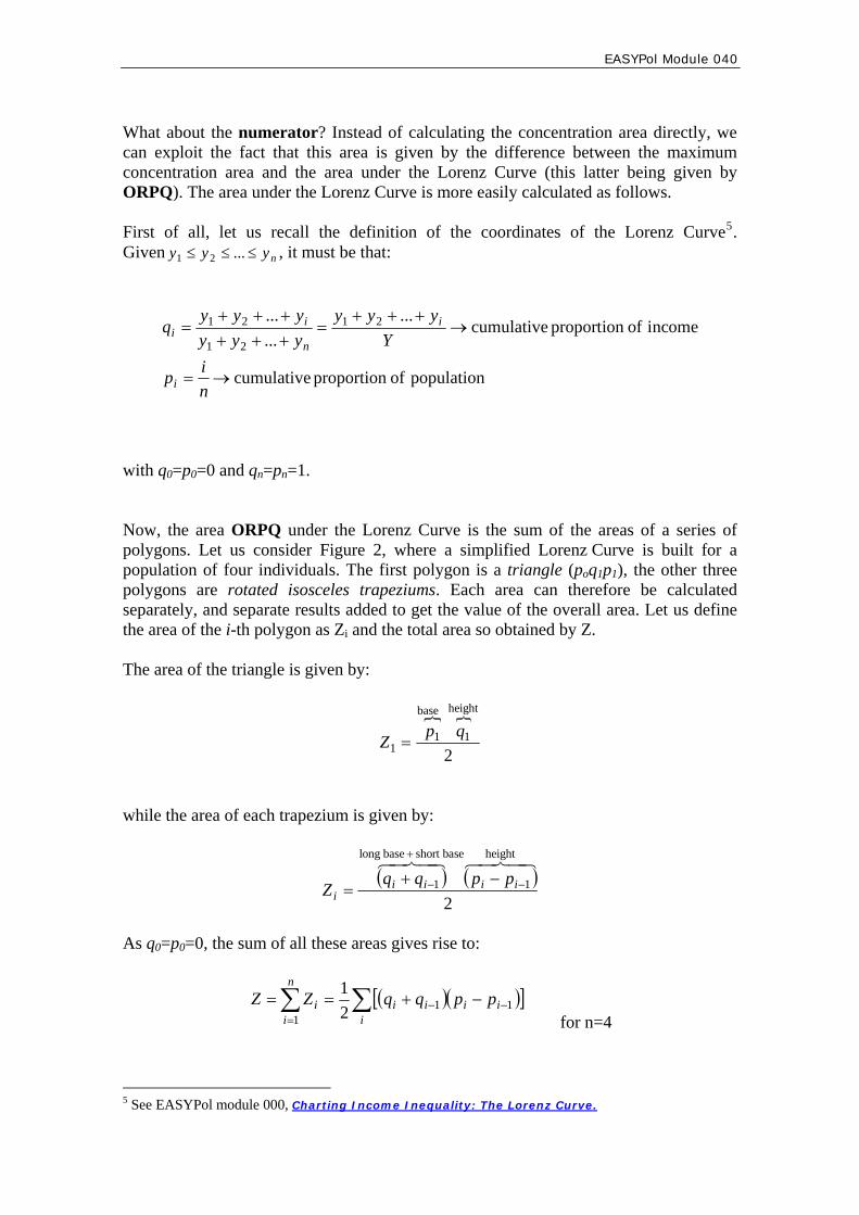
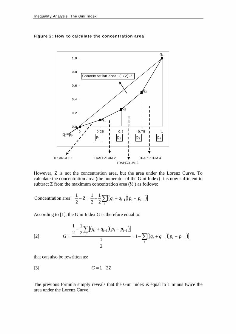
EASYPol Module 040 Analytical Tools
6
This geometrical interpretation based on the Lorenz Curve however is only one of the possible methods to calculate the Gini Index One way that will prove particularly useful below is to directly express the Gini Index in terms of the covariance between income levels and the cumulative distribution of income In particular
( )( )y
yFyCovG 2= [4]
where Cov is the covariance between income levels y and the cumulative distribution of the same income F(y) and y is average income In turn it is worth recalling that the covariance is the expected value E of the products of the deviations from the mean of each variable In the specific case
[ ] [ ] [ ])()()( yFyFyyEyFyCov minussdotminus= [5]
32 The generalised Gini Index (Gv)
In evaluating the policy impact on inequality we have an inequality measure that is flexible enough to embody different policy-makersrsquo preferences with regard to say the degree of inequality aversion After all the effects of a given policy might be evaluated differently by two policy makers having different attitudes towards inequality The Gini Index developed in the previous section (henceforth the standard Gini Index) does not allow for any variation in this attitude ie the degree of inequality aversion A generalisation of the Gini Index by Yitzhaki (1983) makes the Gini index dependent on the specified degree of inequality aversion The corresponding formula is the following
G v( )= minus vy
Cov y 1minus F(y)( )vminus1⎡ ⎣ ⎢
⎤ [6] ⎦ ⎥
where all terms have the same meaning as in [4] and v is the degree of inequality aversion Assigning different values to v may change the value of the Gini Index by weighting differently incomes in different parts of the income distribution Note that with v=2 expression [6] collapses to the standard Gini Index (expression [4]) In order to capture the meaning of the generalised Gini Index let us just recall the following expanded definition of the covariance term in [6]
( )[ ] [ ] ( ) ( )[ ])(1)(1)(1 yFyFyyEyFyCov minusminusminussdotminus=minus [7]
Inequality Analysis The Gini Index 7
The second square bracket on the right hand side of expression [7] is best interpreted as the weight that should be assigned to each income level ie to each deviation from the mean income level (the first square bracket) For lower incomes (below mean income) the first square bracket is negative For lower incomes instead the second square bracket is positive For higher incomes (above the mean) the situation is reversed Deviations from mean incomes are positive while the term in the second square bracket will be negative Note that one property of the cumulative distribution function (CDF) is that its mean is equal to its median value (frac12) Therefore the value in the second square bracket will be positive until the median value of the CDF This means that the median value of the income distribution will have a zero weight as the median income is that income level where F(y) = frac12 We now have to understand what happens to incomes before and after the median when the value of v increases Figure 3 investigates this issue The red line depicts the difference of [1-F(y)] from its mean for the standard case of v=2 The red line intersects the x-axis in correspondence to the median level of this hypothetical income distribution If we now consider the case v=3 (the bold black line) it is relatively easy to see that there is a fraction of richer people (to the right of the intersection with v=2 in the south-east area of the graph) that has (in absolute terms) a lower weight than in v=2 This regards all incomes for which the bold black line lies above the red line in the graph At the same time there is a fraction of poorer people (to the left of the intersection with v=2 in the north-west area of the graph) that has a greater weight than in v=2 This regards all incomes for which the bold black line lies again above the red line in the graph By increasing v the fraction of richer people increases whose income deviation from the mean receives less weight than in v=2 At the same time the fraction of poorer people decreases whose income deviation from the mean receives more weight than in v=2 Figure 3 reports the case for v=2 v=4 v=8 and v=16 Therefore as v increases there is a smaller number of low incomes having a large weight and an increasing number of people having a zero weight In calculating the Gini Index therefore increasing v means focusing more on inequality in a progressively lower fraction of the income distribution6 6 This is the reason why v is often thought of as an laquoinequality aversion parameterraquo
EASYPol Module 040 Analytical Tools
8
Figure 3 Weighting schemes in the Gini Index
-06
-04
-02
00
02
04
06
08
10
Income levels
(1-F
(y))
dev
iations
from
the
mea
n
v=2 v=3 v=4 v=8 v=16
As v increases a progressively increasing set of richer individuals counts less than in v=2At v =16 even some low-income people count zero as the focus is on progressively more extreme poverty
As v increases a progressively decreasing set of poor individuals counts morethan in v =2 The higher v is the more rapidly the weight of individuals decreases At v =16few low-income people count much
Hence the generalised Gini Index gives more flexibility to the evaluation of development programs and policies than the standard Gini Index because of the possibility to embody different degrees of inequality aversion To best interpret this issue it is worth using the example described in Table 1 Table 1 An example of the implicit weighting scheme in the generalised Gini Index
Individuals Incomes F(y) 1-F(y) [1-F(y)]v-
1 v =2
[1-F(y)]v-1
v =4
Incomes deviations from the
mean
[1-F(y)]v-1 v=2
deviations from the
mean
[1-F(y)]v-1 v=4
deviations from the
mean
Implicit weighting
scheme with v=2
Implicit weighting
scheme with v=4
1 1000 020 080 080 051 -2000 040 045 20 80
2 2000 040 060 060 022 -1000 020 015 15 34
3 3000 060 040 040 006 0 000 000 10 10
4 4000 080 020 020 001 1000 -020 -006 05 01
5 5000 100 000 000 000 2000 -040 -006 00 00
Mean 3000 060 040 040 006 Table 1 reports a hypothetical distribution of income with five individuals For each level of income the third and the fourth column report the calculation of F(y) and (1-F(y)) respectively The fifth and the sixth columns give the result of applying v=2 and v=4 to the outcome of the fourth column Note that v=2 corresponds to the standard Gini Index while v=4 should correspond to weighting more people with low incomes
Inequality Analysis The Gini Index 9
The seventh column reports the deviation of each income from average income For low incomes this deviation is negative while it is positive for higher incomes We must just recall that this is a part of the covariance term in [7] The eighth and the ninth columns calculate the deviations from the mean of the other part of the covariance term in formula [7] What should we look for when comparing these columns We can easily see that the laquoweightraquo assigned to the lowest incomes is greater with v=4 than with v=2 At the same time the weight of the richest individual goes rapidly to zero with v=4 One way to derive the implicit weighting scheme of the Gini Index is to set the ratio of the value of the function (1-F(y))v-1 at any income level compared with the value of the same function at the median level of income For v=2 and v=4 this calculation is reported in the last two columns of Table 1 At v=2 twice as much contribution to the calculation of the Gini Index would be attached to the lowest income (compared with the median income) With v=4 eight times as much contribution would instead be attached to the lowest income Also note that the contribution of the highest incomes is lower at v=4
4 A STEP-BY-STEP PROCEDURE TO CALCULATE THE GINI INDEX
41 The Gini Index
To illustrate the step-by-step procedure to build the Gini Index we can refer to Figure 4 Note that this Figure is built by referring to formula [2] above The starting point is to sort the income distribution by income level (Step 1) In Step 2 we must calculate the cumulative income distribution In Step 3 we can obtain the cumulative proportion of income (qi) by dividing each cumulative income by total income Step 4 gives the cumulative proportion of population (pi) We must rank individuals in an increasing order assigning rank 1 to the individual with the lowest income and rank ldquonrdquo to the one with the highest income and then dividing by n In Step 5 we must compute the areas of the polygons Z1Z2 Z3Zn The first one is a triangle the rest are trapeziums (apply the formula in the text) In step 6 all the areas are summed up to obtain the area under the Lorenz Curve (Z) then the Gini Index G=1-2Z is computed Figure 4 presents the usual flow-chart to implement this step-by-step procedure
EASYPol Module 040 Analytical Tools
10
Figure 4 A step-by-step procedure to calculate the Gini Index
STEP Operational content
1If not already sorted sort the income
distribution by income level
2 Calculate the cumulative income distribution
3Calculate the cumulative proportion of income by dividing each cumulative
income by total income
4
By assigning rank 1 to the lowest income and rank n to the highest income calculate the cumulative
proportion of the population by dividing each rank by n
5Compute the area of polygons by
applying formulas for areas of triangle and trapezium in the text
6Sum up all the areas to obtain Z Then
calculate G=1-2Z However an alternative formula to calculate the Gini Index directly has been provided in the text (see formula [4]) based on the covariance term It is therefore worth explaining the step-by-step procedure to calculate the Gini Index in this alternative way Figure 5 illustrates Figure 5 A step-by-step procedure to calculate the Gini Index with the covariance formula
STEP Operational content
1If not already sorted sort the income
distribution by income level
2Calculate the cumulative distribution
function F(y)
3Calculate the covariance Cov(yF(y))
and the mean income level
4 Calculate Gini by applying formula [4] in the text
In particular Step 1 as usual asks us to sort the income distribution by income levels
Inequality Analysis The Gini Index 11
Step 2 asks us to calculate the CDF F(y) 7
Step 3 only asks us to take the covariance between the distribution of income levels and the cumulative distribution function and the mean income level which is used in the denominator of formula [4] Finally Step 4 is the direct application of formula [4] in the text
42 The generalised Gini Index
Figure 6 reports the steps required to calculate the generalised version of the Gini Index Figure 6 A step-by-step procedure to calculate the generalised Gini Index
STEP Operational content
1 If not already sorted sort the income distribution by income level
2 Calculate the cumulative distribution function F(y)
3 For each income calculate 1-F(y)
4 Choose the value of the inequality aversion parameter v
5 Calculate [1-F(y)]v -1
6Calculate the covariance
Cov[y (1-F(y))v -1] and the mean of the income distribution
7 Calculate GINI by applying the covariance formula [6] in the text
The steps are very similar to those required to calculate the standard Gini Index by the covariance formula In particular Step 1 and Step 2 are identical For convenience because of the way in which the formula is expressed Step 3 asks us to calculate for each income level the value of one minus the value of the cumulative distribution function at that point Step 4 is the most characteristic element of this procedure as it asks us to choose the value of the parameter of inequality aversion v We must just recall that higher values of v indicate more inequality aversion
7 See EASYPol Module 007 Impacts of Policies on Poverty Basic Poverty Measures
EASYPol Module 040 Analytical Tools
12
Step 5 asks us to calculate one element of the covariance term namely the value of (1-F(y))v-1 In Step 6 we have to calculate the full covariance and the average income This opens the way to apply formula [6] in the text to get the generalised Gini Index (Step 7)
5 A NUMERICAL EXAMPLE OF HOW TO CALCULATE THE GINI INDEX
51 The standard Gini Index with the Lorenz derivation
The calculation of the Gini Index in its Lorenz Curve derivation may be appreciated by looking at Table 2 In this Table we assume the existence of an income distribution with five individuals (and five incomes) Step 1 just asks us to sort this income distribution by income level Step 2 instead asks us to calculate the cumulative distribution of income The final point of this calculation is therefore 15000 units of income ie total income in the economy Table 2 A numerical example to calculate the Gini Index (Lorenz derivation)
STEP 2 STEP 3 STEP 5 STEP 6
Calculate cumulative
income
Calculate the cumulative
proportion of income (qi)
Assigning rank to incomes
Calculate the cumulative
proportion of population (pi)
Compute the areas of
polygons (Z)
Calculate the Gini index
Individual Income
distributionCumulative
income
Cumulative proportion of
incomeRanks
Cumulative proportion of population
Area of polygons
Gini index
1 0 0 0000 1 02 00002 0 0 0000 2 04 0000 08003 0 0 0000 3 06 00004 0 0 0000 4 08 00005 15000 15000 1000 5 10 0100
0100
STEP 1
Sort the income distribution
STEP 4
Value of Z the area under the Lorenz curve
G = 1 - 2Z
Area of the first triangle
Areas of each
trapezium
Example0027=[(0200+0067)(04-02)]2
0007=[0067 x 02]2
Step 3 transforms the cumulative income distribution into a cumulative proportion of income The final point is now 1 We must just recall that these values are the qirsquos introduced in section 31 above
Inequality Analysis The Gini Index 13
According to the sort of the income distribution made in Step 1 an increasing rank (from 1 to n) is assigned to each income (Step 4) These ranks are then transformed in the cumulative proportion of the population This calculation gives the p rsquos discussed in isection 31 above Having both q and p for all income levels we can calculate the area of the polygons below the Lorenz Curve We must just remember that the first is a triangle and the others are trapeziums Step 5 accomplishes this task by applying the formulas developed in section 31 The sum of all these areas gives Z the total area under the Lorenz Curve Finally Step 6 is the mechanical application of formula [6] in the text The resulting Gini Index is 0267
52 The standard Gini Index with the covariance formula
Table 3 reports a numerical example to calculate the Gini Index according to the covariance formula [4] included in the text In this case the steps are reduced Step 1 is the same as before just sort the income distribution by income level Step 2 asks us to calculate the cumulative distribution function F(y) Step 3 asks us to calculate the two essential parameters to apply the covariance formula the covariance between income levels and the cumulative distribution function (whose value is 400 in the example) and the mean income level which is 3000 income units Table 3 A numerical example to calculate the Gini Index with the covariance formula
STEP 2 STEP 4
Calculate the cumulative distribution
function F(y)
Calculate the covariance Cov
(y F(y))
Calculate the mean income
level
Calculate Gini by using
formula [4]
Individual A - A typical
income distribution
Cumulative income
distributionCovariance Mean income Gini
1 1000 022 2000 043 3000 064 4000 085 5000 10 400 3000 0267
STEP 1
Sort the income distribution
STEP 3
By applying formula [4] in the text we can obtain a value of the Gini Index equal to 0267 (of course the same as in Table 2)
53 The generalised Gini Index
Using the covariance formula we have explained that the standard Gini Index may be made sensitive to a given degree of inequality aversion Table 4 reports an example of
EASYPol Module 040 Analytical Tools
14
how to cope with this generalisation using the same income distribution as in Tables 2 and 3 Table 4 A numerical example to calculate the generalised Gini Index
STEP 2 STEP 3 STEP 4 STEP 5 STEP 7
Calculate the cumulative distribution
function F(y)
Calculate 1 - F(y)
Choose vCalculate
[1 - F(y)](v-1)
Calculate the covariance
Cov (y F(y))
Calculate the mean income
level
Calculate Gini by using
formula [4]
Individual
A - A typical income
distribution
Cumulative income
distribution1 - F(y) v [1 - F(y)](v-1) Covariance
Mean income
Gini
1 1000 02 08 0512 2000 04 06 0223 3000 06 04 0064 4000 08 02 0015 5000 10 00 4 000 -246 3000 0246
STEP 1 STEP 6
Sort the income distribution
Steps 1 and 2 are identical to those already discussed in Table 3 Step 3 instead asks us to calculate the values of one minus the cumulative distribution function Step 4 introduces the parameter of inequality aversion v which we have chosen to be 4 Any amount calculated in Step 3 is therefore raised at the power of (v-1) ie 3 (Step 5) Step 6 calculates the two essential parameters the covariance term (-246 in the example) and the mean income (3000) Step 7 applies formula [6] in the text giving rise to a Gini Index of 0246 Note that this value is different from that obtained with the standard Gini Index as different weights have now been attached to the same incomes
6 THE MAIN PROPERTIES OF THE GINI INDEX
This section will describe the main properties of the Gini Index in terms of the axioms it respects 8
As most of the properties are common to both the standard and the generalised Gini Index the discussion will be carried out under a common heading The main differences among the two indices will however be underlined The main properties of the Gini Index are G has zero as lower limit for any v When all incomes are equal the covariance
between income levels and the cumulative distribution function is zero The Gini Index is therefore zero With regard to the geometrical interpretation of the standard Gini Index note that when all incomes are equal the Lorenz Curve is equal to the equidistribution line Therefore the sum of areas of the polygons (Z) is equal to frac12 ie the sum of the triangle under the Lorenz Curve Therefore the Gini Index (1ndash 2Z) is equal to zero
8 See EASYPol Module 054 Policy Impacts on Inequality Inequality and Axioms for its
Measurement for a discussion of axioms in inequality measurement
Inequality Analysis The Gini Index 15
nn 1minus The standard Gini Index G has as upper limit The limit of this value for
very large populations is 1 When all incomes are zero except for the last the last income is also equal to total income y=Y It means that there is only one area to calculate ie the last trapezium However for very large populations this area tends to be smaller In the limit (ie in a continuous framework) the value of the area Z tends towards zero Therefore the Gini Index tends towards 1 As a
generalisation G(v) has n
nv
12 minus as upper limit Remember that the standard Gini
Index is one in which v=2 The Gini Index is scale invariant By multiplying all incomes by a factor α the
value of the Gini Index G does not change Intuitively when all incomes are scaled by a common factor the cumulative distribution of income does not change as a given fraction of population still holds the same fraction of total income The areas under the Lorenz Curve therefore do not change With regard to the covariance formula the application of a common factor to all incomes makes the covariance and the average income increase by the same factor The Gini Index does not change The same is true for G(v)
On the other hand the Gini Index G is not translation invariant By
addingsubtracting the same amount of money to all incomes the Gini Index would increase (decrease) accordingly The same is true for G(v)
The Gini Index satisfies the principle of transfers for any v If income is
redistributed from relatively richer individuals to relatively poorer individuals both G and G(v) decrease The opposite holds true if income is redistributed from relatively poorer to relatively richer individuals With regard to the standard Gini Index we note that the size of its change following a change in any income depends on the rank of the individuals involved in redistribution and on the sample size It does not depend on the level of individual incomes involved in redistribution but it depends on total income In particular the Gini Index reacts more to redistribution occurring among individuals who have a greater difference in ranks The same amount of redistribution indeed generates a much lower effect if the two individuals have a close rank
Table 5 illustrates how the main properties of the Gini Index work In the left panel of the table there are three simulated income distributions The first is a laquotypical oneraquo ranked by income level The second is where all individuals have the same income The third is where all individuals have zero income except for the last For the typical income distribution A the Gini Index is 0267 For the equi-distributed incomes B the Gini Index is zero while for the most concentrated income distribution
C the Gini Index is 08 ( 80541
==minusn
n )
EASYPol Module 040 Analytical Tools
16
If all incomes were increased by 20 per cent the fifth column of the table shows that the Gini Index would be unchanged (0267) This is the property of scale invariance This is not the case when all incomes are increased by the same absolute amounts (eg 2000 income units in the text) In this case Table 5 shows that the Gini Index would be lower (0160) The Gini Index is not translation invariant The Gini Index satisfies the principle of transfers If we redistribute say 500 income units from the richest to the poorest individuals the Gini Index would be lower (0213) in the text Note that the same transfers when occurring between individuals having closer ranking (the last column of Table 5) still gives rise to a lower Gini Index (0253) but higher than in the previous case (0213) This shows that the Gini Index is more sensitive to transfers occurring among individuals having distant ranks Table 5 The main properties of the Gini Index
Individual A - A typical
income distribution
B - Income distribution with equal incomes
C - Income distribution with
only one individual having income
Original income distribution with
all incomes increased by 20 per cent
Original income distribution with all incomes increased by US$ 2000
Original income distribution with a
redistribution of US$ 500 from the richest
to the poorest
Original income distribution with a
redistribution of US$ 200 from two
individuals with a close rank
1 1000 3000 0 1200 3000 1500 10002 2000 3000 0 2400 4000 2000 25003 3000 3000 0 3600 5000 3000 25004 4000 3000 0 4800 6000 4000 40005 5000 3000 15000 6000 7000 4500 5000
Total income 15000 15000 15000 18000 25000 15000 15000
GINI 0267 0000 0800 0267 0160 0213 0253
UNCHANGED DECREASED DECREASED DECREASED
The Gini index reacts less to transfersamong individuals with a close rank
7 LORENZ INTERSECTION AND THE GINI INDEX
We have explained that the Gini Index may be Lorenz-derived In other terms the Gini Index is Lorenz consistent However it is worth recalling that the ordering provided by Lorenz Curves in particular by Lorenz dominance is a partial ordering as when Lorenz Curves do not cross anything we can say which income distribution has more inequality The Gini Index instead provides for a complete ordering as it reduces the whole income distribution to a single number The basic difference between the two approaches can be appreciated by considering a case in which Lorenz Curves cross For example let us consider the two income distributions reported in Table 6 Incomes are distributed differently but the Gini Index is the same (0200)
Inequality Analysis The Gini Index 17
Table 6 Two income distributions with the same Gini Index
IndividualsIncome
distribution XIncome
distribution Y
1 2000 9002 3000 40003 4000 48004 5000 48005 6000 5500
Total income20000 20000
Gini 0200 0200 These two income distributions give rise to Lorenz Curves as depicted in Figure 7 Lorenz Curves intersect therefore they cannot be used to rank income inequality among these two income distributions But the way they intersect is such that the area before the intersection and the area after the intersection are of the same value This give rise to the same Gini Index even in the presence of quite different income distributions Figure 7 An intersection of Lorenz Curves
00
02
04
06
08
10
00 02 04 06 08 10Dis_X Dis_Y
Different income distributionsLorenz intersectionSame Gini index
Concentration areabefore intersection
Concentration areaafter intersection
EASYPol Module 040 Analytical Tools
18
8 A SYNTHESIS OF THE MAIN PROPERTIES OF THE GINI INDEX AND OF ITS GENERALISED VERSION
Table 7 gives a synthetic picture of the main properties of the Gini Index and its generalised version These properties reflect the structure of axioms 9
It is worth first noting that the lower limit of the both the standard Gini Index and of its generalised version is zero while the higher limit is differentiated The latter limit is very close to 1 (for very large populations) in the case of the standard Gini Index it tends towards 2v (again for very large populations) in the case of the generalised Gini Index Both versions of the Gini Index respect the principle of transfers However it is worth recalling that the Gini Index is more sensible for income transfers among individuals having a wide distance in their relative position (ranks) in the income distribution Both versions are scale invariant and not translation invariant and respect the principle of population This structure makes the Gini Index and the generalised version of the same index two indices belonging to the class of relative inequality indexes In applied works the characteristics of these indices are very useful hence the reason why they merit a high appeal Table 7 The Gini Index and its desirable properties
LOWER LIMIT
UPPER LIMIT
Principle of transfers
Scale invariance
Translation invariance
Principle of population
Index of relative inequality (RII)
Appeal
Gini 0 (n -1)n
YES more sensible if
individuals have distant ranks
YES NO YES YES High
Gv 0 (2v )(n -1)n
YES more sensible if
individuals have distant ranks
YES NO YES YES High
9 READERSrsquo NOTES
91 EASYPol links
Selected EASYPol modules may be used to strengthen readersrsquo background and to further expand their knowledge on inequality and inequality measurement This module belongs to a set of modules that discuss how to compare on inequality grounds alternative income distributions generated by different policy options It is part of the modules composing a training path addressing Analysis and monitoring of socio-economic impacts of policies
9 As discussed in EASYPol Module 054 Policy Impacts on Inequality Inequality and Axioms for its Measurement
Inequality Analysis The Gini Index 19
The following EASYPol modules form a set of materials logically preceding the current module which can be used to strengthen usersrsquo backgrounds
EASYPol Module 000 Charting Income Inequality The Lorenz Curve
EASYPol Module 001 Ranking Income Distribution with Lorenz Curves
EASYPol Module 007 Impacts of Policies on Poverty Basic Poverty Measures
EASYPol Module 054 Policy Impacts on Inequality Inequality and Axioms for its Measurement
Issues addressed in this module are further elaborated in the following modules
EASYPol Module 002 Social Welfare Analysis of Income Distributions Ranking Income Distribution with Generalised Lorenz Curves
EASYPol Module 041 Social Welfare Analysis of Income Distributions Social Welfare Social Welfare Functions and Inequality-Aversion
A case study presenting the use of the Gini Index to measure inequality impacts in the context an agricultural policy impact simulation exercise with real data is reported in the EASYPol Module 042 Inequality and Poverty Impacts of Selected Agricultural Policies The Case of Paraguay
EASYPol Module 040 Analytical Tools
20
10 APPENDIX I ndash ALTERNATIVE WAYS TO CALCULATE THE GINI INDEX
The geometrical derivation of the Gini Index and an alternative formula
The Lorenz derivation of the Gini Index has a direct correspondence with another rather cumbersome way to calculate the Gini Index
⎟⎠
⎞⎜⎝
⎛ ++++⎟⎠⎞
⎜⎝⎛minus+= minusminus
Yy
nY
yY
yYy
nnG nnn 121 32211 [A1]
Note the peculiarity of the last round bracket where each income share from the highest to the lowest is multiplied by the rank of individuals in the income distribution from the lowest to the highest so that the largest share has rank 1 and the smallest share has rank n This correspondence is best shown by an example with n=3 By recalling the definition of qrsquos and prsquos we get
133 1
032
031
0
0300 0
3321
3
221
2
11
1
00
0
===+++
=
=++
=
=+
=
=====
pY
yyyq
pY
yyq
pY
yq
np
Yy
q
By substituting these values into equation [2] in the text would yield
⎥⎦⎤
⎢⎣⎡ ++minus=⎥
⎦
⎤⎢⎣
⎡⎟⎠⎞
⎜⎝⎛ +
+++
+⎟⎠⎞
⎜⎝⎛ +
++minus=
Yy
Yy
Yy
Yyy
Yyyy
Yy
Yyy
YyG 123213211211
1 35
33
311
31
31
311[A2]
Let us call this definition of the Gini Index G1 Now let us also rewrite expression [A1] as
⎥⎦
⎤⎢⎣
⎡ ++minus+=Yy
Yy
Yy
G 1232 32
32
311 [A3]
Let us call this definition of the Gini Inde x G2
Inequality Analysis The Gini Index 21
Now let us rewrite [A2] and [A3] in a more convenient way by manipulating the square brackets
⎥⎦
⎤⎢⎣
⎡ +minusminus=⎥⎦
⎤⎢⎣
⎡++⎟
⎠
⎞⎜⎝
⎛ ++minus=
Yy
Yy
Yy
Yy
Yyyy
G 12121231 2
32
311
34
32
311 [A4]
⎥⎦⎤
⎢⎣⎡ +minusminus=⎥⎦
⎤⎢⎣⎡ +minusminus+=⎥
⎦
⎤⎢⎣
⎡++⎟
⎠⎞
⎜⎝⎛ ++
minus+=Yy
Yy
Yy
Yy
Yy
Yy
YyyyG 121212123
2 232
3112
32
32
3112
32
311[A5]
as the expression in round brackets in both equations is equal to 1 for n=3 It is quite easy to verify that the two expressions give the same result (G =G1 2) The formula [A1] which is often used in operational applications is therefore entirely based on the geometrical derivation of the Gini Index
101 The Gini Index with the covariance formula
In the text we have shown that the Gini Index might be directly calculated if we know the mean income and the covariance between income levels y and the cumulative distribution function F(y) Analytically
( ))(2 yFyCovy
G = [A6]
This formula is also equivalent to formula [A1] Let us see why
( )[ ] ( )[ ])(1 yFyCovyFyCov minusminus=Using the fact that since the expected value of F(y) is frac12 and the expected value of [1-F(y)] is also frac12 we can rewrite the expression [A6] as
( )[ ])(12 yFyCovy
G minusminus=
The equivalence between formula [A6] and formula [A1] can be shown again for a simplified case n=3 First of all it is worth recalling that
where E denotes the expected value (the mean) of a given variable Second it is worth defining the individual components of the covariance
( ) ( ) ( ) ( )()()( yFEyEyyFEyFyCov minus= )
( ) ( ) ( )32
333
32
31
)( 3
3
31
32
33
)(123
=++
==++
= yFEYyEyyy
yyFE
Therefore taking into account that we can yield 321 yyyY ++=
( ) [ ]13123123 9
192
92
92
91
92
93)( yyyyyyyyyFyCov minus=minusminusminus++=
EASYPol Module 040 Analytical Tools
22
nYy =By considering that the covariance formula for Gini Index becomes
[ ] ⎥⎦
⎤⎢⎣
⎡minus=minussdot
sdot=
Yy
Yy
yyY
G 1313 3
29132
Now considering that for n=3
1321 =++
Yyyy expression [A1] can be rewritten
⎥⎦
⎤⎢⎣
⎡minus=minusminusminusminusminusminus⎟
⎠
⎞⎜⎝
⎛ +++++
Yy
Yy
Yy
Yy
Yy
Yy
Yy
Yy
Yyyy
Yy
Yy
Yy 13111223321321
32
32
32
32
32
32
32
31
which is the same as that obtained with the covariance formula
102 The main properties of the Gini Index
GINI HAS ZERO AS A LOWER LIMIT We can see that for the simplified case where n=3 In the specific case Y=3y Then the formula [A1] ] would yield
034
311
36
32
311
3232
311 =minus+=⎟⎟
⎠
⎞⎜⎜⎝
⎛minus+=⎟
⎠
⎞⎜⎝
⎛ ++minus+=yy
Yy
Yy
Yy
G
GINI HAS (N-1)N AS UPPER LIMIT This can again be shown for n=3 to be Assuming again n=3 when all incomes are zero except for the last expression [3b4] would yield
nn
Yy
YYG 1
32
32
31100
32
311 minus
==minus+=⎟⎠⎞
⎜⎝⎛ ++minus+=
as in this case y=Y GINI IS SCALE INVARIANT We can see this by scaling formula [A1] by α For example with n=3 G would
become ⎟⎠⎞
⎜⎝⎛ ++minus+=⎟
⎠⎞
⎜⎝⎛
αα
+α
α+
αα
minus+=Yy
Yy
Yy
Yy
Yy
YyG 323323 32
32
31132
32
311
GINI IS NOT TRANSLATION INVARIANT This can again be seen through equation [A1] in the case of n=3 Suppose all incomes are increased by Δy = $ 2000 which means that total income will be increased by nΔy ie Equation [A1] would become 00023 sdot
Inequality Analysis The Gini Index 23
( ) ( ) ( ) ⎥⎦
⎤⎢⎣
⎡⎟⎟⎠
⎞⎜⎜⎝
⎛sdot+
++⎟⎟
⎠
⎞⎜⎜⎝
⎛sdot+
++⎟⎟
⎠
⎞⎜⎜⎝
⎛sdot+
+minus+=
000230002
3000230002
2000230002
32
311 123
Yy
Yy
Yy
G
As the numerator and the denominator of all round brackets grow in different ways their ratios are different from those of the original formula There is therefore no reason to expect the same Gini Index GINI SATISFIES THE PRINCIPLE OF TRANSFERS This can be easily seen by considering the derivative of the Gini Index with respect to the i-th income
( ) ⎟⎠⎞
⎜⎝⎛minus+⎟
⎠⎞
⎜⎝⎛minus=
partpart
Yin
nyG
i
112
rank individual43421
GINI REACTS LESS TO TRANSFERS OCCURRING AMONG INDIVIDUALS WITH CLOSER RANKS Let us explain this again by assuming n=3 and assuming first that income is redistributed from the richest person (rank 3) to the poorest person (rank 1) By totally differentiating [A1] with respect to y would yield
( ) dyY
dyY
dyY
dG ⎥⎦⎤
⎢⎣⎡minus=minus⎟
⎠⎞
⎜⎝⎛ sdotminus⎟
⎠⎞
⎜⎝⎛ sdotminus=
3411
323
32
31 y decreasing todueG ofvariation y increasing todueG ofvariation 448447648476
Now let us assume that income is redistributed from the richest individual (rank 3) to the immediately less richer individual (rank 2) In this case differentiation would yield
( ) dyY
dyY
dyY
dG ⎥⎦⎤
⎢⎣⎡minus=minus⎟
⎠⎞
⎜⎝⎛ sdotminus⎟
⎠⎞
⎜⎝⎛ sdotminus=
3211
322
32
32 y decreasing todueG ofvariation y increasing todueG ofvariation 448447648476
which is clearly lower than dG in the first case This property can be generalised by saying that given the rank of the donor (in our example from income y3) the reduction of the Gini Index is higher the more distant the rank of the receiver is from that of the donor As a consequence the Gini Index is more sensible to transfers occurring around the mode of the income distribution where there is higher density of individuals
EASYPol Module 040 Analytical Tools
24
11 REFERENCES AND FURTHER READING
Anand S 1983 Inequality and Poverty in Malaysia Oxford University Press London
UK Cowell F 1977 Measuring Inequality Phillip Allan Oxford UK Dalton H 1920 The Measurement of Inequality of Incomes Economic Journal 30 Gini C 1912 Variabilitagrave e mutabilitagrave Bologna Italy Pigou AC 1912 Wealth and Welfare MacMillan London UK Sen AK 1973 On economic Inequality Calarendon Press Oxford UK Theil H 1967 Economics and Information Theory North-Holland Amsterdam The
Netherlands Yitzhaki S 1983 On the Extension of the Gini Index International Economic Review
24 617-628
Inequality Analysis The Gini Index 25
Module metadata
1 EASYPol module 040
2 Title in original language
English Inequality Analysis
French
Spanish
Other language
3 Subtitle in original language
English The Gini Index
French
Spanish
Other language
4 Summary
This tool addresses the most popular inequality index the Gini Index It discusses its characteristics and the link with another popular graphical tool of representing inequality the Lorenz Curve Extended version of the Gini Index with different weighting schemes are also discussed The use of the Gini Index and of its generalised versions is explained through a step-by-step procedure and numerical examples
5 Date
December 2006
6 Author(s)
Lorenzo Giovanni Bellugrave Agricultural Policy Support Service Policy Assistance Division FAO Rome Italy
Paolo Liberati University of Urbino Carlo Bo Institute of Economics Urbino Italy
7 Module type Thematic overview Conceptual and technical materials
Analytical tools Applied materials Complementary resources
8 Topic covered by Agriculture in the macroeconomic context the module Agricultural and sub-sectoral policies Agro-industry and food chain policies
Environment and sustainability Institutional and organizational development Investment planning and policies Poverty and food security Regional integration and international trade Rural Development
9 Subtopics covered by the module
10 Training path Analysis and monitoring of socio-economic impacts of policies
EASYPol Module 040 Analytical Tools
26
11 Keywords capacity building agriculture agricultural policies agricultural development development policies policy analysis policy impact anlaysis poverty food security analytical tool inequality inequality analysis inequality index inequality measures cost-benefit analysis gini index generalised gini index lorenz curve social welfare analysis
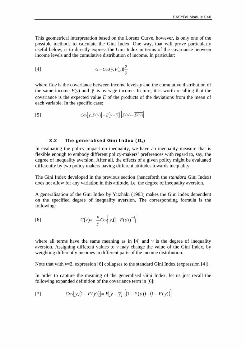
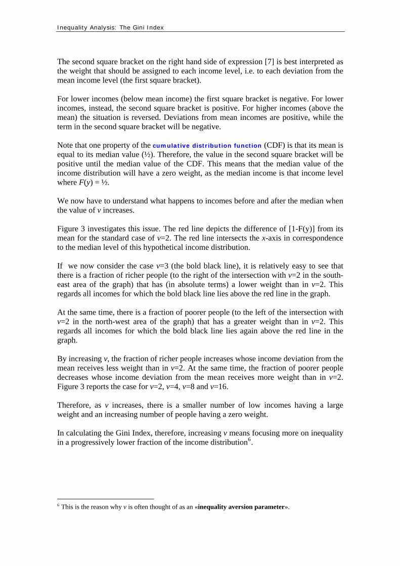
EASYPol Module 040 Analytical Tools
8
Figure 3 Weighting schemes in the Gini Index
-06
-04
-02
00
02
04
06
08
10
Income levels
(1-F
(y))
dev
iations
from
the
mea
n
v=2 v=3 v=4 v=8 v=16
As v increases a progressively increasing set of richer individuals counts less than in v=2At v =16 even some low-income people count zero as the focus is on progressively more extreme poverty
As v increases a progressively decreasing set of poor individuals counts morethan in v =2 The higher v is the more rapidly the weight of individuals decreases At v =16few low-income people count much
Hence the generalised Gini Index gives more flexibility to the evaluation of development programs and policies than the standard Gini Index because of the possibility to embody different degrees of inequality aversion To best interpret this issue it is worth using the example described in Table 1 Table 1 An example of the implicit weighting scheme in the generalised Gini Index
Individuals Incomes F(y) 1-F(y) [1-F(y)]v-
1 v =2
[1-F(y)]v-1
v =4
Incomes deviations from the
mean
[1-F(y)]v-1 v=2
deviations from the
mean
[1-F(y)]v-1 v=4
deviations from the
mean
Implicit weighting
scheme with v=2
Implicit weighting
scheme with v=4
1 1000 020 080 080 051 -2000 040 045 20 80
2 2000 040 060 060 022 -1000 020 015 15 34
3 3000 060 040 040 006 0 000 000 10 10
4 4000 080 020 020 001 1000 -020 -006 05 01
5 5000 100 000 000 000 2000 -040 -006 00 00
Mean 3000 060 040 040 006 Table 1 reports a hypothetical distribution of income with five individuals For each level of income the third and the fourth column report the calculation of F(y) and (1-F(y)) respectively The fifth and the sixth columns give the result of applying v=2 and v=4 to the outcome of the fourth column Note that v=2 corresponds to the standard Gini Index while v=4 should correspond to weighting more people with low incomes
Inequality Analysis The Gini Index 9
The seventh column reports the deviation of each income from average income For low incomes this deviation is negative while it is positive for higher incomes We must just recall that this is a part of the covariance term in [7] The eighth and the ninth columns calculate the deviations from the mean of the other part of the covariance term in formula [7] What should we look for when comparing these columns We can easily see that the laquoweightraquo assigned to the lowest incomes is greater with v=4 than with v=2 At the same time the weight of the richest individual goes rapidly to zero with v=4 One way to derive the implicit weighting scheme of the Gini Index is to set the ratio of the value of the function (1-F(y))v-1 at any income level compared with the value of the same function at the median level of income For v=2 and v=4 this calculation is reported in the last two columns of Table 1 At v=2 twice as much contribution to the calculation of the Gini Index would be attached to the lowest income (compared with the median income) With v=4 eight times as much contribution would instead be attached to the lowest income Also note that the contribution of the highest incomes is lower at v=4
4 A STEP-BY-STEP PROCEDURE TO CALCULATE THE GINI INDEX
41 The Gini Index
To illustrate the step-by-step procedure to build the Gini Index we can refer to Figure 4 Note that this Figure is built by referring to formula [2] above The starting point is to sort the income distribution by income level (Step 1) In Step 2 we must calculate the cumulative income distribution In Step 3 we can obtain the cumulative proportion of income (qi) by dividing each cumulative income by total income Step 4 gives the cumulative proportion of population (pi) We must rank individuals in an increasing order assigning rank 1 to the individual with the lowest income and rank ldquonrdquo to the one with the highest income and then dividing by n In Step 5 we must compute the areas of the polygons Z1Z2 Z3Zn The first one is a triangle the rest are trapeziums (apply the formula in the text) In step 6 all the areas are summed up to obtain the area under the Lorenz Curve (Z) then the Gini Index G=1-2Z is computed Figure 4 presents the usual flow-chart to implement this step-by-step procedure
EASYPol Module 040 Analytical Tools
10
Figure 4 A step-by-step procedure to calculate the Gini Index
STEP Operational content
1If not already sorted sort the income
distribution by income level
2 Calculate the cumulative income distribution
3Calculate the cumulative proportion of income by dividing each cumulative
income by total income
4
By assigning rank 1 to the lowest income and rank n to the highest income calculate the cumulative
proportion of the population by dividing each rank by n
5Compute the area of polygons by
applying formulas for areas of triangle and trapezium in the text
6Sum up all the areas to obtain Z Then
calculate G=1-2Z However an alternative formula to calculate the Gini Index directly has been provided in the text (see formula [4]) based on the covariance term It is therefore worth explaining the step-by-step procedure to calculate the Gini Index in this alternative way Figure 5 illustrates Figure 5 A step-by-step procedure to calculate the Gini Index with the covariance formula
STEP Operational content
1If not already sorted sort the income
distribution by income level
2Calculate the cumulative distribution
function F(y)
3Calculate the covariance Cov(yF(y))
and the mean income level
4 Calculate Gini by applying formula [4] in the text
In particular Step 1 as usual asks us to sort the income distribution by income levels
Inequality Analysis The Gini Index 11
Step 2 asks us to calculate the CDF F(y) 7
Step 3 only asks us to take the covariance between the distribution of income levels and the cumulative distribution function and the mean income level which is used in the denominator of formula [4] Finally Step 4 is the direct application of formula [4] in the text
42 The generalised Gini Index
Figure 6 reports the steps required to calculate the generalised version of the Gini Index Figure 6 A step-by-step procedure to calculate the generalised Gini Index
STEP Operational content
1 If not already sorted sort the income distribution by income level
2 Calculate the cumulative distribution function F(y)
3 For each income calculate 1-F(y)
4 Choose the value of the inequality aversion parameter v
5 Calculate [1-F(y)]v -1
6Calculate the covariance
Cov[y (1-F(y))v -1] and the mean of the income distribution
7 Calculate GINI by applying the covariance formula [6] in the text
The steps are very similar to those required to calculate the standard Gini Index by the covariance formula In particular Step 1 and Step 2 are identical For convenience because of the way in which the formula is expressed Step 3 asks us to calculate for each income level the value of one minus the value of the cumulative distribution function at that point Step 4 is the most characteristic element of this procedure as it asks us to choose the value of the parameter of inequality aversion v We must just recall that higher values of v indicate more inequality aversion
7 See EASYPol Module 007 Impacts of Policies on Poverty Basic Poverty Measures
EASYPol Module 040 Analytical Tools
12
Step 5 asks us to calculate one element of the covariance term namely the value of (1-F(y))v-1 In Step 6 we have to calculate the full covariance and the average income This opens the way to apply formula [6] in the text to get the generalised Gini Index (Step 7)
5 A NUMERICAL EXAMPLE OF HOW TO CALCULATE THE GINI INDEX
51 The standard Gini Index with the Lorenz derivation
The calculation of the Gini Index in its Lorenz Curve derivation may be appreciated by looking at Table 2 In this Table we assume the existence of an income distribution with five individuals (and five incomes) Step 1 just asks us to sort this income distribution by income level Step 2 instead asks us to calculate the cumulative distribution of income The final point of this calculation is therefore 15000 units of income ie total income in the economy Table 2 A numerical example to calculate the Gini Index (Lorenz derivation)
STEP 2 STEP 3 STEP 5 STEP 6
Calculate cumulative
income
Calculate the cumulative
proportion of income (qi)
Assigning rank to incomes
Calculate the cumulative
proportion of population (pi)
Compute the areas of
polygons (Z)
Calculate the Gini index
Individual Income
distributionCumulative
income
Cumulative proportion of
incomeRanks
Cumulative proportion of population
Area of polygons
Gini index
1 0 0 0000 1 02 00002 0 0 0000 2 04 0000 08003 0 0 0000 3 06 00004 0 0 0000 4 08 00005 15000 15000 1000 5 10 0100
0100
STEP 1
Sort the income distribution
STEP 4
Value of Z the area under the Lorenz curve
G = 1 - 2Z
Area of the first triangle
Areas of each
trapezium
Example0027=[(0200+0067)(04-02)]2
0007=[0067 x 02]2
Step 3 transforms the cumulative income distribution into a cumulative proportion of income The final point is now 1 We must just recall that these values are the qirsquos introduced in section 31 above
Inequality Analysis The Gini Index 13
According to the sort of the income distribution made in Step 1 an increasing rank (from 1 to n) is assigned to each income (Step 4) These ranks are then transformed in the cumulative proportion of the population This calculation gives the p rsquos discussed in isection 31 above Having both q and p for all income levels we can calculate the area of the polygons below the Lorenz Curve We must just remember that the first is a triangle and the others are trapeziums Step 5 accomplishes this task by applying the formulas developed in section 31 The sum of all these areas gives Z the total area under the Lorenz Curve Finally Step 6 is the mechanical application of formula [6] in the text The resulting Gini Index is 0267
52 The standard Gini Index with the covariance formula
Table 3 reports a numerical example to calculate the Gini Index according to the covariance formula [4] included in the text In this case the steps are reduced Step 1 is the same as before just sort the income distribution by income level Step 2 asks us to calculate the cumulative distribution function F(y) Step 3 asks us to calculate the two essential parameters to apply the covariance formula the covariance between income levels and the cumulative distribution function (whose value is 400 in the example) and the mean income level which is 3000 income units Table 3 A numerical example to calculate the Gini Index with the covariance formula
STEP 2 STEP 4
Calculate the cumulative distribution
function F(y)
Calculate the covariance Cov
(y F(y))
Calculate the mean income
level
Calculate Gini by using
formula [4]
Individual A - A typical
income distribution
Cumulative income
distributionCovariance Mean income Gini
1 1000 022 2000 043 3000 064 4000 085 5000 10 400 3000 0267
STEP 1
Sort the income distribution
STEP 3
By applying formula [4] in the text we can obtain a value of the Gini Index equal to 0267 (of course the same as in Table 2)
53 The generalised Gini Index
Using the covariance formula we have explained that the standard Gini Index may be made sensitive to a given degree of inequality aversion Table 4 reports an example of
EASYPol Module 040 Analytical Tools
14
how to cope with this generalisation using the same income distribution as in Tables 2 and 3 Table 4 A numerical example to calculate the generalised Gini Index
STEP 2 STEP 3 STEP 4 STEP 5 STEP 7
Calculate the cumulative distribution
function F(y)
Calculate 1 - F(y)
Choose vCalculate
[1 - F(y)](v-1)
Calculate the covariance
Cov (y F(y))
Calculate the mean income
level
Calculate Gini by using
formula [4]
Individual
A - A typical income
distribution
Cumulative income
distribution1 - F(y) v [1 - F(y)](v-1) Covariance
Mean income
Gini
1 1000 02 08 0512 2000 04 06 0223 3000 06 04 0064 4000 08 02 0015 5000 10 00 4 000 -246 3000 0246
STEP 1 STEP 6
Sort the income distribution
Steps 1 and 2 are identical to those already discussed in Table 3 Step 3 instead asks us to calculate the values of one minus the cumulative distribution function Step 4 introduces the parameter of inequality aversion v which we have chosen to be 4 Any amount calculated in Step 3 is therefore raised at the power of (v-1) ie 3 (Step 5) Step 6 calculates the two essential parameters the covariance term (-246 in the example) and the mean income (3000) Step 7 applies formula [6] in the text giving rise to a Gini Index of 0246 Note that this value is different from that obtained with the standard Gini Index as different weights have now been attached to the same incomes
6 THE MAIN PROPERTIES OF THE GINI INDEX
This section will describe the main properties of the Gini Index in terms of the axioms it respects 8
As most of the properties are common to both the standard and the generalised Gini Index the discussion will be carried out under a common heading The main differences among the two indices will however be underlined The main properties of the Gini Index are G has zero as lower limit for any v When all incomes are equal the covariance
between income levels and the cumulative distribution function is zero The Gini Index is therefore zero With regard to the geometrical interpretation of the standard Gini Index note that when all incomes are equal the Lorenz Curve is equal to the equidistribution line Therefore the sum of areas of the polygons (Z) is equal to frac12 ie the sum of the triangle under the Lorenz Curve Therefore the Gini Index (1ndash 2Z) is equal to zero
8 See EASYPol Module 054 Policy Impacts on Inequality Inequality and Axioms for its
Measurement for a discussion of axioms in inequality measurement
Inequality Analysis The Gini Index 15
nn 1minus The standard Gini Index G has as upper limit The limit of this value for
very large populations is 1 When all incomes are zero except for the last the last income is also equal to total income y=Y It means that there is only one area to calculate ie the last trapezium However for very large populations this area tends to be smaller In the limit (ie in a continuous framework) the value of the area Z tends towards zero Therefore the Gini Index tends towards 1 As a
generalisation G(v) has n
nv
12 minus as upper limit Remember that the standard Gini
Index is one in which v=2 The Gini Index is scale invariant By multiplying all incomes by a factor α the
value of the Gini Index G does not change Intuitively when all incomes are scaled by a common factor the cumulative distribution of income does not change as a given fraction of population still holds the same fraction of total income The areas under the Lorenz Curve therefore do not change With regard to the covariance formula the application of a common factor to all incomes makes the covariance and the average income increase by the same factor The Gini Index does not change The same is true for G(v)
On the other hand the Gini Index G is not translation invariant By
addingsubtracting the same amount of money to all incomes the Gini Index would increase (decrease) accordingly The same is true for G(v)
The Gini Index satisfies the principle of transfers for any v If income is
redistributed from relatively richer individuals to relatively poorer individuals both G and G(v) decrease The opposite holds true if income is redistributed from relatively poorer to relatively richer individuals With regard to the standard Gini Index we note that the size of its change following a change in any income depends on the rank of the individuals involved in redistribution and on the sample size It does not depend on the level of individual incomes involved in redistribution but it depends on total income In particular the Gini Index reacts more to redistribution occurring among individuals who have a greater difference in ranks The same amount of redistribution indeed generates a much lower effect if the two individuals have a close rank
Table 5 illustrates how the main properties of the Gini Index work In the left panel of the table there are three simulated income distributions The first is a laquotypical oneraquo ranked by income level The second is where all individuals have the same income The third is where all individuals have zero income except for the last For the typical income distribution A the Gini Index is 0267 For the equi-distributed incomes B the Gini Index is zero while for the most concentrated income distribution
C the Gini Index is 08 ( 80541
==minusn
n )
EASYPol Module 040 Analytical Tools
16
If all incomes were increased by 20 per cent the fifth column of the table shows that the Gini Index would be unchanged (0267) This is the property of scale invariance This is not the case when all incomes are increased by the same absolute amounts (eg 2000 income units in the text) In this case Table 5 shows that the Gini Index would be lower (0160) The Gini Index is not translation invariant The Gini Index satisfies the principle of transfers If we redistribute say 500 income units from the richest to the poorest individuals the Gini Index would be lower (0213) in the text Note that the same transfers when occurring between individuals having closer ranking (the last column of Table 5) still gives rise to a lower Gini Index (0253) but higher than in the previous case (0213) This shows that the Gini Index is more sensitive to transfers occurring among individuals having distant ranks Table 5 The main properties of the Gini Index
Individual A - A typical
income distribution
B - Income distribution with equal incomes
C - Income distribution with
only one individual having income
Original income distribution with
all incomes increased by 20 per cent
Original income distribution with all incomes increased by US$ 2000
Original income distribution with a
redistribution of US$ 500 from the richest
to the poorest
Original income distribution with a
redistribution of US$ 200 from two
individuals with a close rank
1 1000 3000 0 1200 3000 1500 10002 2000 3000 0 2400 4000 2000 25003 3000 3000 0 3600 5000 3000 25004 4000 3000 0 4800 6000 4000 40005 5000 3000 15000 6000 7000 4500 5000
Total income 15000 15000 15000 18000 25000 15000 15000
GINI 0267 0000 0800 0267 0160 0213 0253
UNCHANGED DECREASED DECREASED DECREASED
The Gini index reacts less to transfersamong individuals with a close rank
7 LORENZ INTERSECTION AND THE GINI INDEX
We have explained that the Gini Index may be Lorenz-derived In other terms the Gini Index is Lorenz consistent However it is worth recalling that the ordering provided by Lorenz Curves in particular by Lorenz dominance is a partial ordering as when Lorenz Curves do not cross anything we can say which income distribution has more inequality The Gini Index instead provides for a complete ordering as it reduces the whole income distribution to a single number The basic difference between the two approaches can be appreciated by considering a case in which Lorenz Curves cross For example let us consider the two income distributions reported in Table 6 Incomes are distributed differently but the Gini Index is the same (0200)
Inequality Analysis The Gini Index 17
Table 6 Two income distributions with the same Gini Index
IndividualsIncome
distribution XIncome
distribution Y
1 2000 9002 3000 40003 4000 48004 5000 48005 6000 5500
Total income20000 20000
Gini 0200 0200 These two income distributions give rise to Lorenz Curves as depicted in Figure 7 Lorenz Curves intersect therefore they cannot be used to rank income inequality among these two income distributions But the way they intersect is such that the area before the intersection and the area after the intersection are of the same value This give rise to the same Gini Index even in the presence of quite different income distributions Figure 7 An intersection of Lorenz Curves
00
02
04
06
08
10
00 02 04 06 08 10Dis_X Dis_Y
Different income distributionsLorenz intersectionSame Gini index
Concentration areabefore intersection
Concentration areaafter intersection
EASYPol Module 040 Analytical Tools
18
8 A SYNTHESIS OF THE MAIN PROPERTIES OF THE GINI INDEX AND OF ITS GENERALISED VERSION
Table 7 gives a synthetic picture of the main properties of the Gini Index and its generalised version These properties reflect the structure of axioms 9
It is worth first noting that the lower limit of the both the standard Gini Index and of its generalised version is zero while the higher limit is differentiated The latter limit is very close to 1 (for very large populations) in the case of the standard Gini Index it tends towards 2v (again for very large populations) in the case of the generalised Gini Index Both versions of the Gini Index respect the principle of transfers However it is worth recalling that the Gini Index is more sensible for income transfers among individuals having a wide distance in their relative position (ranks) in the income distribution Both versions are scale invariant and not translation invariant and respect the principle of population This structure makes the Gini Index and the generalised version of the same index two indices belonging to the class of relative inequality indexes In applied works the characteristics of these indices are very useful hence the reason why they merit a high appeal Table 7 The Gini Index and its desirable properties
LOWER LIMIT
UPPER LIMIT
Principle of transfers
Scale invariance
Translation invariance
Principle of population
Index of relative inequality (RII)
Appeal
Gini 0 (n -1)n
YES more sensible if
individuals have distant ranks
YES NO YES YES High
Gv 0 (2v )(n -1)n
YES more sensible if
individuals have distant ranks
YES NO YES YES High
9 READERSrsquo NOTES
91 EASYPol links
Selected EASYPol modules may be used to strengthen readersrsquo background and to further expand their knowledge on inequality and inequality measurement This module belongs to a set of modules that discuss how to compare on inequality grounds alternative income distributions generated by different policy options It is part of the modules composing a training path addressing Analysis and monitoring of socio-economic impacts of policies
9 As discussed in EASYPol Module 054 Policy Impacts on Inequality Inequality and Axioms for its Measurement
Inequality Analysis The Gini Index 19
The following EASYPol modules form a set of materials logically preceding the current module which can be used to strengthen usersrsquo backgrounds
EASYPol Module 000 Charting Income Inequality The Lorenz Curve
EASYPol Module 001 Ranking Income Distribution with Lorenz Curves
EASYPol Module 007 Impacts of Policies on Poverty Basic Poverty Measures
EASYPol Module 054 Policy Impacts on Inequality Inequality and Axioms for its Measurement
Issues addressed in this module are further elaborated in the following modules
EASYPol Module 002 Social Welfare Analysis of Income Distributions Ranking Income Distribution with Generalised Lorenz Curves
EASYPol Module 041 Social Welfare Analysis of Income Distributions Social Welfare Social Welfare Functions and Inequality-Aversion
A case study presenting the use of the Gini Index to measure inequality impacts in the context an agricultural policy impact simulation exercise with real data is reported in the EASYPol Module 042 Inequality and Poverty Impacts of Selected Agricultural Policies The Case of Paraguay
EASYPol Module 040 Analytical Tools
20
10 APPENDIX I ndash ALTERNATIVE WAYS TO CALCULATE THE GINI INDEX
The geometrical derivation of the Gini Index and an alternative formula
The Lorenz derivation of the Gini Index has a direct correspondence with another rather cumbersome way to calculate the Gini Index
⎟⎠
⎞⎜⎝
⎛ ++++⎟⎠⎞
⎜⎝⎛minus+= minusminus
Yy
nY
yY
yYy
nnG nnn 121 32211 [A1]
Note the peculiarity of the last round bracket where each income share from the highest to the lowest is multiplied by the rank of individuals in the income distribution from the lowest to the highest so that the largest share has rank 1 and the smallest share has rank n This correspondence is best shown by an example with n=3 By recalling the definition of qrsquos and prsquos we get
133 1
032
031
0
0300 0
3321
3
221
2
11
1
00
0
===+++
=
=++
=
=+
=
=====
pY
yyyq
pY
yyq
pY
yq
np
Yy
q
By substituting these values into equation [2] in the text would yield
⎥⎦⎤
⎢⎣⎡ ++minus=⎥
⎦
⎤⎢⎣
⎡⎟⎠⎞
⎜⎝⎛ +
+++
+⎟⎠⎞
⎜⎝⎛ +
++minus=
Yy
Yy
Yy
Yyy
Yyyy
Yy
Yyy
YyG 123213211211
1 35
33
311
31
31
311[A2]
Let us call this definition of the Gini Index G1 Now let us also rewrite expression [A1] as
⎥⎦
⎤⎢⎣
⎡ ++minus+=Yy
Yy
Yy
G 1232 32
32
311 [A3]
Let us call this definition of the Gini Inde x G2
Inequality Analysis The Gini Index 21
Now let us rewrite [A2] and [A3] in a more convenient way by manipulating the square brackets
⎥⎦
⎤⎢⎣
⎡ +minusminus=⎥⎦
⎤⎢⎣
⎡++⎟
⎠
⎞⎜⎝
⎛ ++minus=
Yy
Yy
Yy
Yy
Yyyy
G 12121231 2
32
311
34
32
311 [A4]
⎥⎦⎤
⎢⎣⎡ +minusminus=⎥⎦
⎤⎢⎣⎡ +minusminus+=⎥
⎦
⎤⎢⎣
⎡++⎟
⎠⎞
⎜⎝⎛ ++
minus+=Yy
Yy
Yy
Yy
Yy
Yy
YyyyG 121212123
2 232
3112
32
32
3112
32
311[A5]
as the expression in round brackets in both equations is equal to 1 for n=3 It is quite easy to verify that the two expressions give the same result (G =G1 2) The formula [A1] which is often used in operational applications is therefore entirely based on the geometrical derivation of the Gini Index
101 The Gini Index with the covariance formula
In the text we have shown that the Gini Index might be directly calculated if we know the mean income and the covariance between income levels y and the cumulative distribution function F(y) Analytically
( ))(2 yFyCovy
G = [A6]
This formula is also equivalent to formula [A1] Let us see why
( )[ ] ( )[ ])(1 yFyCovyFyCov minusminus=Using the fact that since the expected value of F(y) is frac12 and the expected value of [1-F(y)] is also frac12 we can rewrite the expression [A6] as
( )[ ])(12 yFyCovy
G minusminus=
The equivalence between formula [A6] and formula [A1] can be shown again for a simplified case n=3 First of all it is worth recalling that
where E denotes the expected value (the mean) of a given variable Second it is worth defining the individual components of the covariance
( ) ( ) ( ) ( )()()( yFEyEyyFEyFyCov minus= )
( ) ( ) ( )32
333
32
31
)( 3
3
31
32
33
)(123
=++
==++
= yFEYyEyyy
yyFE
Therefore taking into account that we can yield 321 yyyY ++=
( ) [ ]13123123 9
192
92
92
91
92
93)( yyyyyyyyyFyCov minus=minusminusminus++=
EASYPol Module 040 Analytical Tools
22
nYy =By considering that the covariance formula for Gini Index becomes
[ ] ⎥⎦
⎤⎢⎣
⎡minus=minussdot
sdot=
Yy
Yy
yyY
G 1313 3
29132
Now considering that for n=3
1321 =++
Yyyy expression [A1] can be rewritten
⎥⎦
⎤⎢⎣
⎡minus=minusminusminusminusminusminus⎟
⎠
⎞⎜⎝
⎛ +++++
Yy
Yy
Yy
Yy
Yy
Yy
Yy
Yy
Yyyy
Yy
Yy
Yy 13111223321321
32
32
32
32
32
32
32
31
which is the same as that obtained with the covariance formula
102 The main properties of the Gini Index
GINI HAS ZERO AS A LOWER LIMIT We can see that for the simplified case where n=3 In the specific case Y=3y Then the formula [A1] ] would yield
034
311
36
32
311
3232
311 =minus+=⎟⎟
⎠
⎞⎜⎜⎝
⎛minus+=⎟
⎠
⎞⎜⎝
⎛ ++minus+=yy
Yy
Yy
Yy
G
GINI HAS (N-1)N AS UPPER LIMIT This can again be shown for n=3 to be Assuming again n=3 when all incomes are zero except for the last expression [3b4] would yield
nn
Yy
YYG 1
32
32
31100
32
311 minus
==minus+=⎟⎠⎞
⎜⎝⎛ ++minus+=
as in this case y=Y GINI IS SCALE INVARIANT We can see this by scaling formula [A1] by α For example with n=3 G would
become ⎟⎠⎞
⎜⎝⎛ ++minus+=⎟
⎠⎞
⎜⎝⎛
αα
+α
α+
αα
minus+=Yy
Yy
Yy
Yy
Yy
YyG 323323 32
32
31132
32
311
GINI IS NOT TRANSLATION INVARIANT This can again be seen through equation [A1] in the case of n=3 Suppose all incomes are increased by Δy = $ 2000 which means that total income will be increased by nΔy ie Equation [A1] would become 00023 sdot
Inequality Analysis The Gini Index 23
( ) ( ) ( ) ⎥⎦
⎤⎢⎣
⎡⎟⎟⎠
⎞⎜⎜⎝
⎛sdot+
++⎟⎟
⎠
⎞⎜⎜⎝
⎛sdot+
++⎟⎟
⎠
⎞⎜⎜⎝
⎛sdot+
+minus+=
000230002
3000230002
2000230002
32
311 123
Yy
Yy
Yy
G
As the numerator and the denominator of all round brackets grow in different ways their ratios are different from those of the original formula There is therefore no reason to expect the same Gini Index GINI SATISFIES THE PRINCIPLE OF TRANSFERS This can be easily seen by considering the derivative of the Gini Index with respect to the i-th income
( ) ⎟⎠⎞
⎜⎝⎛minus+⎟
⎠⎞
⎜⎝⎛minus=
partpart
Yin
nyG
i
112
rank individual43421
GINI REACTS LESS TO TRANSFERS OCCURRING AMONG INDIVIDUALS WITH CLOSER RANKS Let us explain this again by assuming n=3 and assuming first that income is redistributed from the richest person (rank 3) to the poorest person (rank 1) By totally differentiating [A1] with respect to y would yield
( ) dyY
dyY
dyY
dG ⎥⎦⎤
⎢⎣⎡minus=minus⎟
⎠⎞
⎜⎝⎛ sdotminus⎟
⎠⎞
⎜⎝⎛ sdotminus=
3411
323
32
31 y decreasing todueG ofvariation y increasing todueG ofvariation 448447648476
Now let us assume that income is redistributed from the richest individual (rank 3) to the immediately less richer individual (rank 2) In this case differentiation would yield
( ) dyY
dyY
dyY
dG ⎥⎦⎤
⎢⎣⎡minus=minus⎟
⎠⎞
⎜⎝⎛ sdotminus⎟
⎠⎞
⎜⎝⎛ sdotminus=
3211
322
32
32 y decreasing todueG ofvariation y increasing todueG ofvariation 448447648476
which is clearly lower than dG in the first case This property can be generalised by saying that given the rank of the donor (in our example from income y3) the reduction of the Gini Index is higher the more distant the rank of the receiver is from that of the donor As a consequence the Gini Index is more sensible to transfers occurring around the mode of the income distribution where there is higher density of individuals
EASYPol Module 040 Analytical Tools
24
11 REFERENCES AND FURTHER READING
Anand S 1983 Inequality and Poverty in Malaysia Oxford University Press London
UK Cowell F 1977 Measuring Inequality Phillip Allan Oxford UK Dalton H 1920 The Measurement of Inequality of Incomes Economic Journal 30 Gini C 1912 Variabilitagrave e mutabilitagrave Bologna Italy Pigou AC 1912 Wealth and Welfare MacMillan London UK Sen AK 1973 On economic Inequality Calarendon Press Oxford UK Theil H 1967 Economics and Information Theory North-Holland Amsterdam The
Netherlands Yitzhaki S 1983 On the Extension of the Gini Index International Economic Review
24 617-628
Inequality Analysis The Gini Index 25
Module metadata
1 EASYPol module 040
2 Title in original language
English Inequality Analysis
French
Spanish
Other language
3 Subtitle in original language
English The Gini Index
French
Spanish
Other language
4 Summary
This tool addresses the most popular inequality index the Gini Index It discusses its characteristics and the link with another popular graphical tool of representing inequality the Lorenz Curve Extended version of the Gini Index with different weighting schemes are also discussed The use of the Gini Index and of its generalised versions is explained through a step-by-step procedure and numerical examples
5 Date
December 2006
6 Author(s)
Lorenzo Giovanni Bellugrave Agricultural Policy Support Service Policy Assistance Division FAO Rome Italy
Paolo Liberati University of Urbino Carlo Bo Institute of Economics Urbino Italy
7 Module type Thematic overview Conceptual and technical materials
Analytical tools Applied materials Complementary resources
8 Topic covered by Agriculture in the macroeconomic context the module Agricultural and sub-sectoral policies Agro-industry and food chain policies
Environment and sustainability Institutional and organizational development Investment planning and policies Poverty and food security Regional integration and international trade Rural Development
9 Subtopics covered by the module
10 Training path Analysis and monitoring of socio-economic impacts of policies
EASYPol Module 040 Analytical Tools
26
11 Keywords capacity building agriculture agricultural policies agricultural development development policies policy analysis policy impact anlaysis poverty food security analytical tool inequality inequality analysis inequality index inequality measures cost-benefit analysis gini index generalised gini index lorenz curve social welfare analysis
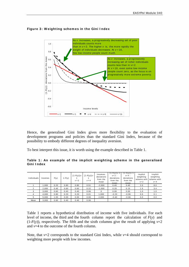
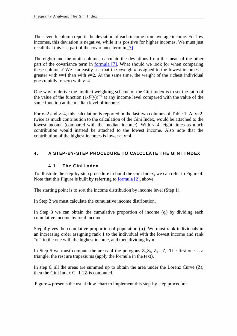
EASYPol Module 040 Analytical Tools
10
Figure 4 A step-by-step procedure to calculate the Gini Index
STEP Operational content
1If not already sorted sort the income
distribution by income level
2 Calculate the cumulative income distribution
3Calculate the cumulative proportion of income by dividing each cumulative
income by total income
4
By assigning rank 1 to the lowest income and rank n to the highest income calculate the cumulative
proportion of the population by dividing each rank by n
5Compute the area of polygons by
applying formulas for areas of triangle and trapezium in the text
6Sum up all the areas to obtain Z Then
calculate G=1-2Z However an alternative formula to calculate the Gini Index directly has been provided in the text (see formula [4]) based on the covariance term It is therefore worth explaining the step-by-step procedure to calculate the Gini Index in this alternative way Figure 5 illustrates Figure 5 A step-by-step procedure to calculate the Gini Index with the covariance formula
STEP Operational content
1If not already sorted sort the income
distribution by income level
2Calculate the cumulative distribution
function F(y)
3Calculate the covariance Cov(yF(y))
and the mean income level
4 Calculate Gini by applying formula [4] in the text
In particular Step 1 as usual asks us to sort the income distribution by income levels
Inequality Analysis The Gini Index 11
Step 2 asks us to calculate the CDF F(y) 7
Step 3 only asks us to take the covariance between the distribution of income levels and the cumulative distribution function and the mean income level which is used in the denominator of formula [4] Finally Step 4 is the direct application of formula [4] in the text
42 The generalised Gini Index
Figure 6 reports the steps required to calculate the generalised version of the Gini Index Figure 6 A step-by-step procedure to calculate the generalised Gini Index
STEP Operational content
1 If not already sorted sort the income distribution by income level
2 Calculate the cumulative distribution function F(y)
3 For each income calculate 1-F(y)
4 Choose the value of the inequality aversion parameter v
5 Calculate [1-F(y)]v -1
6Calculate the covariance
Cov[y (1-F(y))v -1] and the mean of the income distribution
7 Calculate GINI by applying the covariance formula [6] in the text
The steps are very similar to those required to calculate the standard Gini Index by the covariance formula In particular Step 1 and Step 2 are identical For convenience because of the way in which the formula is expressed Step 3 asks us to calculate for each income level the value of one minus the value of the cumulative distribution function at that point Step 4 is the most characteristic element of this procedure as it asks us to choose the value of the parameter of inequality aversion v We must just recall that higher values of v indicate more inequality aversion
7 See EASYPol Module 007 Impacts of Policies on Poverty Basic Poverty Measures
EASYPol Module 040 Analytical Tools
12
Step 5 asks us to calculate one element of the covariance term namely the value of (1-F(y))v-1 In Step 6 we have to calculate the full covariance and the average income This opens the way to apply formula [6] in the text to get the generalised Gini Index (Step 7)
5 A NUMERICAL EXAMPLE OF HOW TO CALCULATE THE GINI INDEX
51 The standard Gini Index with the Lorenz derivation
The calculation of the Gini Index in its Lorenz Curve derivation may be appreciated by looking at Table 2 In this Table we assume the existence of an income distribution with five individuals (and five incomes) Step 1 just asks us to sort this income distribution by income level Step 2 instead asks us to calculate the cumulative distribution of income The final point of this calculation is therefore 15000 units of income ie total income in the economy Table 2 A numerical example to calculate the Gini Index (Lorenz derivation)
STEP 2 STEP 3 STEP 5 STEP 6
Calculate cumulative
income
Calculate the cumulative
proportion of income (qi)
Assigning rank to incomes
Calculate the cumulative
proportion of population (pi)
Compute the areas of
polygons (Z)
Calculate the Gini index
Individual Income
distributionCumulative
income
Cumulative proportion of
incomeRanks
Cumulative proportion of population
Area of polygons
Gini index
1 0 0 0000 1 02 00002 0 0 0000 2 04 0000 08003 0 0 0000 3 06 00004 0 0 0000 4 08 00005 15000 15000 1000 5 10 0100
0100
STEP 1
Sort the income distribution
STEP 4
Value of Z the area under the Lorenz curve
G = 1 - 2Z
Area of the first triangle
Areas of each
trapezium
Example0027=[(0200+0067)(04-02)]2
0007=[0067 x 02]2
Step 3 transforms the cumulative income distribution into a cumulative proportion of income The final point is now 1 We must just recall that these values are the qirsquos introduced in section 31 above
Inequality Analysis The Gini Index 13
According to the sort of the income distribution made in Step 1 an increasing rank (from 1 to n) is assigned to each income (Step 4) These ranks are then transformed in the cumulative proportion of the population This calculation gives the p rsquos discussed in isection 31 above Having both q and p for all income levels we can calculate the area of the polygons below the Lorenz Curve We must just remember that the first is a triangle and the others are trapeziums Step 5 accomplishes this task by applying the formulas developed in section 31 The sum of all these areas gives Z the total area under the Lorenz Curve Finally Step 6 is the mechanical application of formula [6] in the text The resulting Gini Index is 0267
52 The standard Gini Index with the covariance formula
Table 3 reports a numerical example to calculate the Gini Index according to the covariance formula [4] included in the text In this case the steps are reduced Step 1 is the same as before just sort the income distribution by income level Step 2 asks us to calculate the cumulative distribution function F(y) Step 3 asks us to calculate the two essential parameters to apply the covariance formula the covariance between income levels and the cumulative distribution function (whose value is 400 in the example) and the mean income level which is 3000 income units Table 3 A numerical example to calculate the Gini Index with the covariance formula
STEP 2 STEP 4
Calculate the cumulative distribution
function F(y)
Calculate the covariance Cov
(y F(y))
Calculate the mean income
level
Calculate Gini by using
formula [4]
Individual A - A typical
income distribution
Cumulative income
distributionCovariance Mean income Gini
1 1000 022 2000 043 3000 064 4000 085 5000 10 400 3000 0267
STEP 1
Sort the income distribution
STEP 3
By applying formula [4] in the text we can obtain a value of the Gini Index equal to 0267 (of course the same as in Table 2)
53 The generalised Gini Index
Using the covariance formula we have explained that the standard Gini Index may be made sensitive to a given degree of inequality aversion Table 4 reports an example of
EASYPol Module 040 Analytical Tools
14
how to cope with this generalisation using the same income distribution as in Tables 2 and 3 Table 4 A numerical example to calculate the generalised Gini Index
STEP 2 STEP 3 STEP 4 STEP 5 STEP 7
Calculate the cumulative distribution
function F(y)
Calculate 1 - F(y)
Choose vCalculate
[1 - F(y)](v-1)
Calculate the covariance
Cov (y F(y))
Calculate the mean income
level
Calculate Gini by using
formula [4]
Individual
A - A typical income
distribution
Cumulative income
distribution1 - F(y) v [1 - F(y)](v-1) Covariance
Mean income
Gini
1 1000 02 08 0512 2000 04 06 0223 3000 06 04 0064 4000 08 02 0015 5000 10 00 4 000 -246 3000 0246
STEP 1 STEP 6
Sort the income distribution
Steps 1 and 2 are identical to those already discussed in Table 3 Step 3 instead asks us to calculate the values of one minus the cumulative distribution function Step 4 introduces the parameter of inequality aversion v which we have chosen to be 4 Any amount calculated in Step 3 is therefore raised at the power of (v-1) ie 3 (Step 5) Step 6 calculates the two essential parameters the covariance term (-246 in the example) and the mean income (3000) Step 7 applies formula [6] in the text giving rise to a Gini Index of 0246 Note that this value is different from that obtained with the standard Gini Index as different weights have now been attached to the same incomes
6 THE MAIN PROPERTIES OF THE GINI INDEX
This section will describe the main properties of the Gini Index in terms of the axioms it respects 8
As most of the properties are common to both the standard and the generalised Gini Index the discussion will be carried out under a common heading The main differences among the two indices will however be underlined The main properties of the Gini Index are G has zero as lower limit for any v When all incomes are equal the covariance
between income levels and the cumulative distribution function is zero The Gini Index is therefore zero With regard to the geometrical interpretation of the standard Gini Index note that when all incomes are equal the Lorenz Curve is equal to the equidistribution line Therefore the sum of areas of the polygons (Z) is equal to frac12 ie the sum of the triangle under the Lorenz Curve Therefore the Gini Index (1ndash 2Z) is equal to zero
8 See EASYPol Module 054 Policy Impacts on Inequality Inequality and Axioms for its
Measurement for a discussion of axioms in inequality measurement
Inequality Analysis The Gini Index 15
nn 1minus The standard Gini Index G has as upper limit The limit of this value for
very large populations is 1 When all incomes are zero except for the last the last income is also equal to total income y=Y It means that there is only one area to calculate ie the last trapezium However for very large populations this area tends to be smaller In the limit (ie in a continuous framework) the value of the area Z tends towards zero Therefore the Gini Index tends towards 1 As a
generalisation G(v) has n
nv
12 minus as upper limit Remember that the standard Gini
Index is one in which v=2 The Gini Index is scale invariant By multiplying all incomes by a factor α the
value of the Gini Index G does not change Intuitively when all incomes are scaled by a common factor the cumulative distribution of income does not change as a given fraction of population still holds the same fraction of total income The areas under the Lorenz Curve therefore do not change With regard to the covariance formula the application of a common factor to all incomes makes the covariance and the average income increase by the same factor The Gini Index does not change The same is true for G(v)
On the other hand the Gini Index G is not translation invariant By
addingsubtracting the same amount of money to all incomes the Gini Index would increase (decrease) accordingly The same is true for G(v)
The Gini Index satisfies the principle of transfers for any v If income is
redistributed from relatively richer individuals to relatively poorer individuals both G and G(v) decrease The opposite holds true if income is redistributed from relatively poorer to relatively richer individuals With regard to the standard Gini Index we note that the size of its change following a change in any income depends on the rank of the individuals involved in redistribution and on the sample size It does not depend on the level of individual incomes involved in redistribution but it depends on total income In particular the Gini Index reacts more to redistribution occurring among individuals who have a greater difference in ranks The same amount of redistribution indeed generates a much lower effect if the two individuals have a close rank
Table 5 illustrates how the main properties of the Gini Index work In the left panel of the table there are three simulated income distributions The first is a laquotypical oneraquo ranked by income level The second is where all individuals have the same income The third is where all individuals have zero income except for the last For the typical income distribution A the Gini Index is 0267 For the equi-distributed incomes B the Gini Index is zero while for the most concentrated income distribution
C the Gini Index is 08 ( 80541
==minusn
n )
EASYPol Module 040 Analytical Tools
16
If all incomes were increased by 20 per cent the fifth column of the table shows that the Gini Index would be unchanged (0267) This is the property of scale invariance This is not the case when all incomes are increased by the same absolute amounts (eg 2000 income units in the text) In this case Table 5 shows that the Gini Index would be lower (0160) The Gini Index is not translation invariant The Gini Index satisfies the principle of transfers If we redistribute say 500 income units from the richest to the poorest individuals the Gini Index would be lower (0213) in the text Note that the same transfers when occurring between individuals having closer ranking (the last column of Table 5) still gives rise to a lower Gini Index (0253) but higher than in the previous case (0213) This shows that the Gini Index is more sensitive to transfers occurring among individuals having distant ranks Table 5 The main properties of the Gini Index
Individual A - A typical
income distribution
B - Income distribution with equal incomes
C - Income distribution with
only one individual having income
Original income distribution with
all incomes increased by 20 per cent
Original income distribution with all incomes increased by US$ 2000
Original income distribution with a
redistribution of US$ 500 from the richest
to the poorest
Original income distribution with a
redistribution of US$ 200 from two
individuals with a close rank
1 1000 3000 0 1200 3000 1500 10002 2000 3000 0 2400 4000 2000 25003 3000 3000 0 3600 5000 3000 25004 4000 3000 0 4800 6000 4000 40005 5000 3000 15000 6000 7000 4500 5000
Total income 15000 15000 15000 18000 25000 15000 15000
GINI 0267 0000 0800 0267 0160 0213 0253
UNCHANGED DECREASED DECREASED DECREASED
The Gini index reacts less to transfersamong individuals with a close rank
7 LORENZ INTERSECTION AND THE GINI INDEX
We have explained that the Gini Index may be Lorenz-derived In other terms the Gini Index is Lorenz consistent However it is worth recalling that the ordering provided by Lorenz Curves in particular by Lorenz dominance is a partial ordering as when Lorenz Curves do not cross anything we can say which income distribution has more inequality The Gini Index instead provides for a complete ordering as it reduces the whole income distribution to a single number The basic difference between the two approaches can be appreciated by considering a case in which Lorenz Curves cross For example let us consider the two income distributions reported in Table 6 Incomes are distributed differently but the Gini Index is the same (0200)
Inequality Analysis The Gini Index 17
Table 6 Two income distributions with the same Gini Index
IndividualsIncome
distribution XIncome
distribution Y
1 2000 9002 3000 40003 4000 48004 5000 48005 6000 5500
Total income20000 20000
Gini 0200 0200 These two income distributions give rise to Lorenz Curves as depicted in Figure 7 Lorenz Curves intersect therefore they cannot be used to rank income inequality among these two income distributions But the way they intersect is such that the area before the intersection and the area after the intersection are of the same value This give rise to the same Gini Index even in the presence of quite different income distributions Figure 7 An intersection of Lorenz Curves
00
02
04
06
08
10
00 02 04 06 08 10Dis_X Dis_Y
Different income distributionsLorenz intersectionSame Gini index
Concentration areabefore intersection
Concentration areaafter intersection
EASYPol Module 040 Analytical Tools
18
8 A SYNTHESIS OF THE MAIN PROPERTIES OF THE GINI INDEX AND OF ITS GENERALISED VERSION
Table 7 gives a synthetic picture of the main properties of the Gini Index and its generalised version These properties reflect the structure of axioms 9
It is worth first noting that the lower limit of the both the standard Gini Index and of its generalised version is zero while the higher limit is differentiated The latter limit is very close to 1 (for very large populations) in the case of the standard Gini Index it tends towards 2v (again for very large populations) in the case of the generalised Gini Index Both versions of the Gini Index respect the principle of transfers However it is worth recalling that the Gini Index is more sensible for income transfers among individuals having a wide distance in their relative position (ranks) in the income distribution Both versions are scale invariant and not translation invariant and respect the principle of population This structure makes the Gini Index and the generalised version of the same index two indices belonging to the class of relative inequality indexes In applied works the characteristics of these indices are very useful hence the reason why they merit a high appeal Table 7 The Gini Index and its desirable properties
LOWER LIMIT
UPPER LIMIT
Principle of transfers
Scale invariance
Translation invariance
Principle of population
Index of relative inequality (RII)
Appeal
Gini 0 (n -1)n
YES more sensible if
individuals have distant ranks
YES NO YES YES High
Gv 0 (2v )(n -1)n
YES more sensible if
individuals have distant ranks
YES NO YES YES High
9 READERSrsquo NOTES
91 EASYPol links
Selected EASYPol modules may be used to strengthen readersrsquo background and to further expand their knowledge on inequality and inequality measurement This module belongs to a set of modules that discuss how to compare on inequality grounds alternative income distributions generated by different policy options It is part of the modules composing a training path addressing Analysis and monitoring of socio-economic impacts of policies
9 As discussed in EASYPol Module 054 Policy Impacts on Inequality Inequality and Axioms for its Measurement
Inequality Analysis The Gini Index 19
The following EASYPol modules form a set of materials logically preceding the current module which can be used to strengthen usersrsquo backgrounds
EASYPol Module 000 Charting Income Inequality The Lorenz Curve
EASYPol Module 001 Ranking Income Distribution with Lorenz Curves
EASYPol Module 007 Impacts of Policies on Poverty Basic Poverty Measures
EASYPol Module 054 Policy Impacts on Inequality Inequality and Axioms for its Measurement
Issues addressed in this module are further elaborated in the following modules
EASYPol Module 002 Social Welfare Analysis of Income Distributions Ranking Income Distribution with Generalised Lorenz Curves
EASYPol Module 041 Social Welfare Analysis of Income Distributions Social Welfare Social Welfare Functions and Inequality-Aversion
A case study presenting the use of the Gini Index to measure inequality impacts in the context an agricultural policy impact simulation exercise with real data is reported in the EASYPol Module 042 Inequality and Poverty Impacts of Selected Agricultural Policies The Case of Paraguay
EASYPol Module 040 Analytical Tools
20
10 APPENDIX I ndash ALTERNATIVE WAYS TO CALCULATE THE GINI INDEX
The geometrical derivation of the Gini Index and an alternative formula
The Lorenz derivation of the Gini Index has a direct correspondence with another rather cumbersome way to calculate the Gini Index
⎟⎠
⎞⎜⎝
⎛ ++++⎟⎠⎞
⎜⎝⎛minus+= minusminus
Yy
nY
yY
yYy
nnG nnn 121 32211 [A1]
Note the peculiarity of the last round bracket where each income share from the highest to the lowest is multiplied by the rank of individuals in the income distribution from the lowest to the highest so that the largest share has rank 1 and the smallest share has rank n This correspondence is best shown by an example with n=3 By recalling the definition of qrsquos and prsquos we get
133 1
032
031
0
0300 0
3321
3
221
2
11
1
00
0
===+++
=
=++
=
=+
=
=====
pY
yyyq
pY
yyq
pY
yq
np
Yy
q
By substituting these values into equation [2] in the text would yield
⎥⎦⎤
⎢⎣⎡ ++minus=⎥
⎦
⎤⎢⎣
⎡⎟⎠⎞
⎜⎝⎛ +
+++
+⎟⎠⎞
⎜⎝⎛ +
++minus=
Yy
Yy
Yy
Yyy
Yyyy
Yy
Yyy
YyG 123213211211
1 35
33
311
31
31
311[A2]
Let us call this definition of the Gini Index G1 Now let us also rewrite expression [A1] as
⎥⎦
⎤⎢⎣
⎡ ++minus+=Yy
Yy
Yy
G 1232 32
32
311 [A3]
Let us call this definition of the Gini Inde x G2
Inequality Analysis The Gini Index 21
Now let us rewrite [A2] and [A3] in a more convenient way by manipulating the square brackets
⎥⎦
⎤⎢⎣
⎡ +minusminus=⎥⎦
⎤⎢⎣
⎡++⎟
⎠
⎞⎜⎝
⎛ ++minus=
Yy
Yy
Yy
Yy
Yyyy
G 12121231 2
32
311
34
32
311 [A4]
⎥⎦⎤
⎢⎣⎡ +minusminus=⎥⎦
⎤⎢⎣⎡ +minusminus+=⎥
⎦
⎤⎢⎣
⎡++⎟
⎠⎞
⎜⎝⎛ ++
minus+=Yy
Yy
Yy
Yy
Yy
Yy
YyyyG 121212123
2 232
3112
32
32
3112
32
311[A5]
as the expression in round brackets in both equations is equal to 1 for n=3 It is quite easy to verify that the two expressions give the same result (G =G1 2) The formula [A1] which is often used in operational applications is therefore entirely based on the geometrical derivation of the Gini Index
101 The Gini Index with the covariance formula
In the text we have shown that the Gini Index might be directly calculated if we know the mean income and the covariance between income levels y and the cumulative distribution function F(y) Analytically
( ))(2 yFyCovy
G = [A6]
This formula is also equivalent to formula [A1] Let us see why
( )[ ] ( )[ ])(1 yFyCovyFyCov minusminus=Using the fact that since the expected value of F(y) is frac12 and the expected value of [1-F(y)] is also frac12 we can rewrite the expression [A6] as
( )[ ])(12 yFyCovy
G minusminus=
The equivalence between formula [A6] and formula [A1] can be shown again for a simplified case n=3 First of all it is worth recalling that
where E denotes the expected value (the mean) of a given variable Second it is worth defining the individual components of the covariance
( ) ( ) ( ) ( )()()( yFEyEyyFEyFyCov minus= )
( ) ( ) ( )32
333
32
31
)( 3
3
31
32
33
)(123
=++
==++
= yFEYyEyyy
yyFE
Therefore taking into account that we can yield 321 yyyY ++=
( ) [ ]13123123 9
192
92
92
91
92
93)( yyyyyyyyyFyCov minus=minusminusminus++=
EASYPol Module 040 Analytical Tools
22
nYy =By considering that the covariance formula for Gini Index becomes
[ ] ⎥⎦
⎤⎢⎣
⎡minus=minussdot
sdot=
Yy
Yy
yyY
G 1313 3
29132
Now considering that for n=3
1321 =++
Yyyy expression [A1] can be rewritten
⎥⎦
⎤⎢⎣
⎡minus=minusminusminusminusminusminus⎟
⎠
⎞⎜⎝
⎛ +++++
Yy
Yy
Yy
Yy
Yy
Yy
Yy
Yy
Yyyy
Yy
Yy
Yy 13111223321321
32
32
32
32
32
32
32
31
which is the same as that obtained with the covariance formula
102 The main properties of the Gini Index
GINI HAS ZERO AS A LOWER LIMIT We can see that for the simplified case where n=3 In the specific case Y=3y Then the formula [A1] ] would yield
034
311
36
32
311
3232
311 =minus+=⎟⎟
⎠
⎞⎜⎜⎝
⎛minus+=⎟
⎠
⎞⎜⎝
⎛ ++minus+=yy
Yy
Yy
Yy
G
GINI HAS (N-1)N AS UPPER LIMIT This can again be shown for n=3 to be Assuming again n=3 when all incomes are zero except for the last expression [3b4] would yield
nn
Yy
YYG 1
32
32
31100
32
311 minus
==minus+=⎟⎠⎞
⎜⎝⎛ ++minus+=
as in this case y=Y GINI IS SCALE INVARIANT We can see this by scaling formula [A1] by α For example with n=3 G would
become ⎟⎠⎞
⎜⎝⎛ ++minus+=⎟
⎠⎞
⎜⎝⎛
αα
+α
α+
αα
minus+=Yy
Yy
Yy
Yy
Yy
YyG 323323 32
32
31132
32
311
GINI IS NOT TRANSLATION INVARIANT This can again be seen through equation [A1] in the case of n=3 Suppose all incomes are increased by Δy = $ 2000 which means that total income will be increased by nΔy ie Equation [A1] would become 00023 sdot
Inequality Analysis The Gini Index 23
( ) ( ) ( ) ⎥⎦
⎤⎢⎣
⎡⎟⎟⎠
⎞⎜⎜⎝
⎛sdot+
++⎟⎟
⎠
⎞⎜⎜⎝
⎛sdot+
++⎟⎟
⎠
⎞⎜⎜⎝
⎛sdot+
+minus+=
000230002
3000230002
2000230002
32
311 123
Yy
Yy
Yy
G
As the numerator and the denominator of all round brackets grow in different ways their ratios are different from those of the original formula There is therefore no reason to expect the same Gini Index GINI SATISFIES THE PRINCIPLE OF TRANSFERS This can be easily seen by considering the derivative of the Gini Index with respect to the i-th income
( ) ⎟⎠⎞
⎜⎝⎛minus+⎟
⎠⎞
⎜⎝⎛minus=
partpart
Yin
nyG
i
112
rank individual43421
GINI REACTS LESS TO TRANSFERS OCCURRING AMONG INDIVIDUALS WITH CLOSER RANKS Let us explain this again by assuming n=3 and assuming first that income is redistributed from the richest person (rank 3) to the poorest person (rank 1) By totally differentiating [A1] with respect to y would yield
( ) dyY
dyY
dyY
dG ⎥⎦⎤
⎢⎣⎡minus=minus⎟
⎠⎞
⎜⎝⎛ sdotminus⎟
⎠⎞
⎜⎝⎛ sdotminus=
3411
323
32
31 y decreasing todueG ofvariation y increasing todueG ofvariation 448447648476
Now let us assume that income is redistributed from the richest individual (rank 3) to the immediately less richer individual (rank 2) In this case differentiation would yield
( ) dyY
dyY
dyY
dG ⎥⎦⎤
⎢⎣⎡minus=minus⎟
⎠⎞
⎜⎝⎛ sdotminus⎟
⎠⎞
⎜⎝⎛ sdotminus=
3211
322
32
32 y decreasing todueG ofvariation y increasing todueG ofvariation 448447648476
which is clearly lower than dG in the first case This property can be generalised by saying that given the rank of the donor (in our example from income y3) the reduction of the Gini Index is higher the more distant the rank of the receiver is from that of the donor As a consequence the Gini Index is more sensible to transfers occurring around the mode of the income distribution where there is higher density of individuals
EASYPol Module 040 Analytical Tools
24
11 REFERENCES AND FURTHER READING
Anand S 1983 Inequality and Poverty in Malaysia Oxford University Press London
UK Cowell F 1977 Measuring Inequality Phillip Allan Oxford UK Dalton H 1920 The Measurement of Inequality of Incomes Economic Journal 30 Gini C 1912 Variabilitagrave e mutabilitagrave Bologna Italy Pigou AC 1912 Wealth and Welfare MacMillan London UK Sen AK 1973 On economic Inequality Calarendon Press Oxford UK Theil H 1967 Economics and Information Theory North-Holland Amsterdam The
Netherlands Yitzhaki S 1983 On the Extension of the Gini Index International Economic Review
24 617-628
Inequality Analysis The Gini Index 25
Module metadata
1 EASYPol module 040
2 Title in original language
English Inequality Analysis
French
Spanish
Other language
3 Subtitle in original language
English The Gini Index
French
Spanish
Other language
4 Summary
This tool addresses the most popular inequality index the Gini Index It discusses its characteristics and the link with another popular graphical tool of representing inequality the Lorenz Curve Extended version of the Gini Index with different weighting schemes are also discussed The use of the Gini Index and of its generalised versions is explained through a step-by-step procedure and numerical examples
5 Date
December 2006
6 Author(s)
Lorenzo Giovanni Bellugrave Agricultural Policy Support Service Policy Assistance Division FAO Rome Italy
Paolo Liberati University of Urbino Carlo Bo Institute of Economics Urbino Italy
7 Module type Thematic overview Conceptual and technical materials
Analytical tools Applied materials Complementary resources
8 Topic covered by Agriculture in the macroeconomic context the module Agricultural and sub-sectoral policies Agro-industry and food chain policies
Environment and sustainability Institutional and organizational development Investment planning and policies Poverty and food security Regional integration and international trade Rural Development
9 Subtopics covered by the module
10 Training path Analysis and monitoring of socio-economic impacts of policies
EASYPol Module 040 Analytical Tools
26
11 Keywords capacity building agriculture agricultural policies agricultural development development policies policy analysis policy impact anlaysis poverty food security analytical tool inequality inequality analysis inequality index inequality measures cost-benefit analysis gini index generalised gini index lorenz curve social welfare analysis
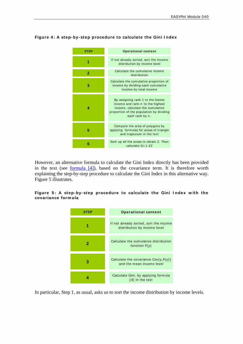
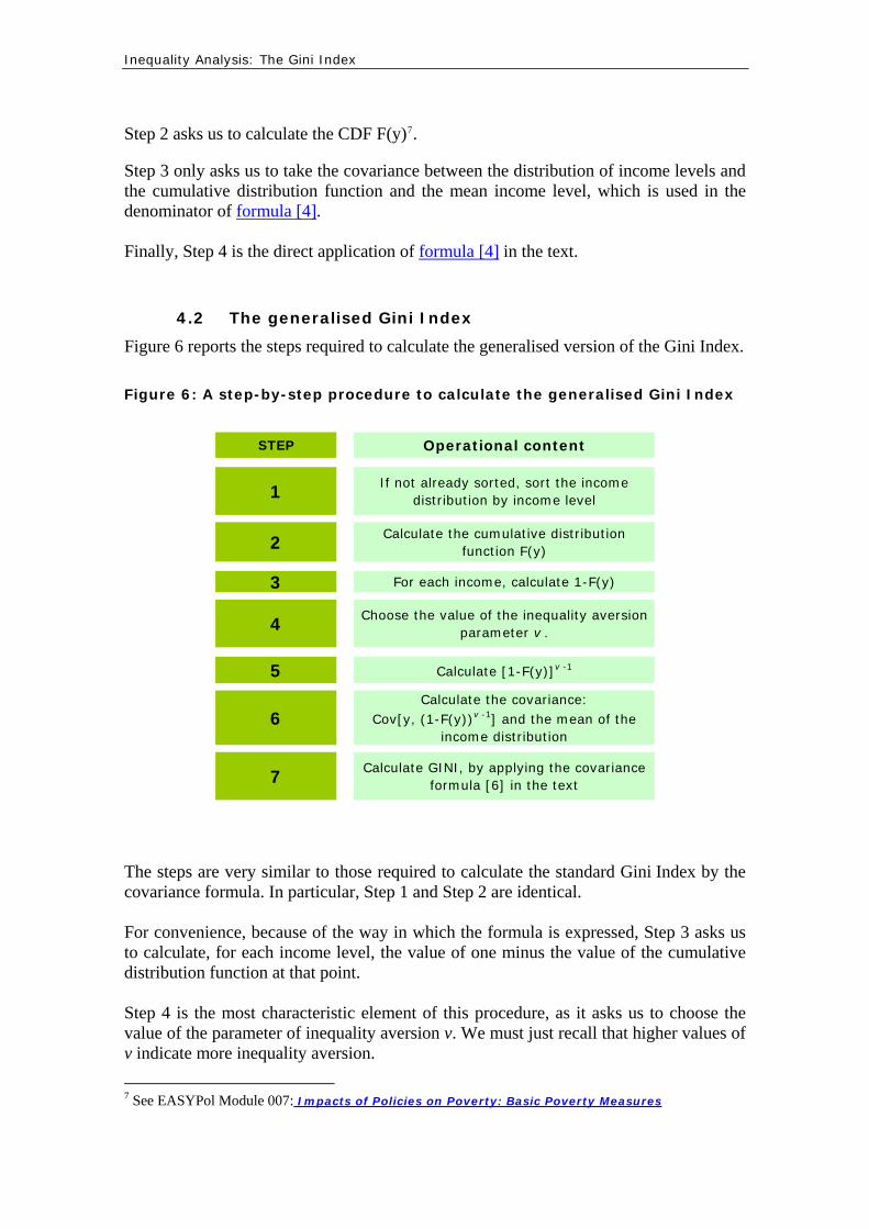
EASYPol Module 040 Analytical Tools
12
Step 5 asks us to calculate one element of the covariance term namely the value of (1-F(y))v-1 In Step 6 we have to calculate the full covariance and the average income This opens the way to apply formula [6] in the text to get the generalised Gini Index (Step 7)
5 A NUMERICAL EXAMPLE OF HOW TO CALCULATE THE GINI INDEX
51 The standard Gini Index with the Lorenz derivation
The calculation of the Gini Index in its Lorenz Curve derivation may be appreciated by looking at Table 2 In this Table we assume the existence of an income distribution with five individuals (and five incomes) Step 1 just asks us to sort this income distribution by income level Step 2 instead asks us to calculate the cumulative distribution of income The final point of this calculation is therefore 15000 units of income ie total income in the economy Table 2 A numerical example to calculate the Gini Index (Lorenz derivation)
STEP 2 STEP 3 STEP 5 STEP 6
Calculate cumulative
income
Calculate the cumulative
proportion of income (qi)
Assigning rank to incomes
Calculate the cumulative
proportion of population (pi)
Compute the areas of
polygons (Z)
Calculate the Gini index
Individual Income
distributionCumulative
income
Cumulative proportion of
incomeRanks
Cumulative proportion of population
Area of polygons
Gini index
1 0 0 0000 1 02 00002 0 0 0000 2 04 0000 08003 0 0 0000 3 06 00004 0 0 0000 4 08 00005 15000 15000 1000 5 10 0100
0100
STEP 1
Sort the income distribution
STEP 4
Value of Z the area under the Lorenz curve
G = 1 - 2Z
Area of the first triangle
Areas of each
trapezium
Example0027=[(0200+0067)(04-02)]2
0007=[0067 x 02]2
Step 3 transforms the cumulative income distribution into a cumulative proportion of income The final point is now 1 We must just recall that these values are the qirsquos introduced in section 31 above
Inequality Analysis The Gini Index 13
According to the sort of the income distribution made in Step 1 an increasing rank (from 1 to n) is assigned to each income (Step 4) These ranks are then transformed in the cumulative proportion of the population This calculation gives the p rsquos discussed in isection 31 above Having both q and p for all income levels we can calculate the area of the polygons below the Lorenz Curve We must just remember that the first is a triangle and the others are trapeziums Step 5 accomplishes this task by applying the formulas developed in section 31 The sum of all these areas gives Z the total area under the Lorenz Curve Finally Step 6 is the mechanical application of formula [6] in the text The resulting Gini Index is 0267
52 The standard Gini Index with the covariance formula
Table 3 reports a numerical example to calculate the Gini Index according to the covariance formula [4] included in the text In this case the steps are reduced Step 1 is the same as before just sort the income distribution by income level Step 2 asks us to calculate the cumulative distribution function F(y) Step 3 asks us to calculate the two essential parameters to apply the covariance formula the covariance between income levels and the cumulative distribution function (whose value is 400 in the example) and the mean income level which is 3000 income units Table 3 A numerical example to calculate the Gini Index with the covariance formula
STEP 2 STEP 4
Calculate the cumulative distribution
function F(y)
Calculate the covariance Cov
(y F(y))
Calculate the mean income
level
Calculate Gini by using
formula [4]
Individual A - A typical
income distribution
Cumulative income
distributionCovariance Mean income Gini
1 1000 022 2000 043 3000 064 4000 085 5000 10 400 3000 0267
STEP 1
Sort the income distribution
STEP 3
By applying formula [4] in the text we can obtain a value of the Gini Index equal to 0267 (of course the same as in Table 2)
53 The generalised Gini Index
Using the covariance formula we have explained that the standard Gini Index may be made sensitive to a given degree of inequality aversion Table 4 reports an example of
EASYPol Module 040 Analytical Tools
14
how to cope with this generalisation using the same income distribution as in Tables 2 and 3 Table 4 A numerical example to calculate the generalised Gini Index
STEP 2 STEP 3 STEP 4 STEP 5 STEP 7
Calculate the cumulative distribution
function F(y)
Calculate 1 - F(y)
Choose vCalculate
[1 - F(y)](v-1)
Calculate the covariance
Cov (y F(y))
Calculate the mean income
level
Calculate Gini by using
formula [4]
Individual
A - A typical income
distribution
Cumulative income
distribution1 - F(y) v [1 - F(y)](v-1) Covariance
Mean income
Gini
1 1000 02 08 0512 2000 04 06 0223 3000 06 04 0064 4000 08 02 0015 5000 10 00 4 000 -246 3000 0246
STEP 1 STEP 6
Sort the income distribution
Steps 1 and 2 are identical to those already discussed in Table 3 Step 3 instead asks us to calculate the values of one minus the cumulative distribution function Step 4 introduces the parameter of inequality aversion v which we have chosen to be 4 Any amount calculated in Step 3 is therefore raised at the power of (v-1) ie 3 (Step 5) Step 6 calculates the two essential parameters the covariance term (-246 in the example) and the mean income (3000) Step 7 applies formula [6] in the text giving rise to a Gini Index of 0246 Note that this value is different from that obtained with the standard Gini Index as different weights have now been attached to the same incomes
6 THE MAIN PROPERTIES OF THE GINI INDEX
This section will describe the main properties of the Gini Index in terms of the axioms it respects 8
As most of the properties are common to both the standard and the generalised Gini Index the discussion will be carried out under a common heading The main differences among the two indices will however be underlined The main properties of the Gini Index are G has zero as lower limit for any v When all incomes are equal the covariance
between income levels and the cumulative distribution function is zero The Gini Index is therefore zero With regard to the geometrical interpretation of the standard Gini Index note that when all incomes are equal the Lorenz Curve is equal to the equidistribution line Therefore the sum of areas of the polygons (Z) is equal to frac12 ie the sum of the triangle under the Lorenz Curve Therefore the Gini Index (1ndash 2Z) is equal to zero
8 See EASYPol Module 054 Policy Impacts on Inequality Inequality and Axioms for its
Measurement for a discussion of axioms in inequality measurement
Inequality Analysis The Gini Index 15
nn 1minus The standard Gini Index G has as upper limit The limit of this value for
very large populations is 1 When all incomes are zero except for the last the last income is also equal to total income y=Y It means that there is only one area to calculate ie the last trapezium However for very large populations this area tends to be smaller In the limit (ie in a continuous framework) the value of the area Z tends towards zero Therefore the Gini Index tends towards 1 As a
generalisation G(v) has n
nv
12 minus as upper limit Remember that the standard Gini
Index is one in which v=2 The Gini Index is scale invariant By multiplying all incomes by a factor α the
value of the Gini Index G does not change Intuitively when all incomes are scaled by a common factor the cumulative distribution of income does not change as a given fraction of population still holds the same fraction of total income The areas under the Lorenz Curve therefore do not change With regard to the covariance formula the application of a common factor to all incomes makes the covariance and the average income increase by the same factor The Gini Index does not change The same is true for G(v)
On the other hand the Gini Index G is not translation invariant By
addingsubtracting the same amount of money to all incomes the Gini Index would increase (decrease) accordingly The same is true for G(v)
The Gini Index satisfies the principle of transfers for any v If income is
redistributed from relatively richer individuals to relatively poorer individuals both G and G(v) decrease The opposite holds true if income is redistributed from relatively poorer to relatively richer individuals With regard to the standard Gini Index we note that the size of its change following a change in any income depends on the rank of the individuals involved in redistribution and on the sample size It does not depend on the level of individual incomes involved in redistribution but it depends on total income In particular the Gini Index reacts more to redistribution occurring among individuals who have a greater difference in ranks The same amount of redistribution indeed generates a much lower effect if the two individuals have a close rank
Table 5 illustrates how the main properties of the Gini Index work In the left panel of the table there are three simulated income distributions The first is a laquotypical oneraquo ranked by income level The second is where all individuals have the same income The third is where all individuals have zero income except for the last For the typical income distribution A the Gini Index is 0267 For the equi-distributed incomes B the Gini Index is zero while for the most concentrated income distribution
C the Gini Index is 08 ( 80541
==minusn
n )
EASYPol Module 040 Analytical Tools
16
If all incomes were increased by 20 per cent the fifth column of the table shows that the Gini Index would be unchanged (0267) This is the property of scale invariance This is not the case when all incomes are increased by the same absolute amounts (eg 2000 income units in the text) In this case Table 5 shows that the Gini Index would be lower (0160) The Gini Index is not translation invariant The Gini Index satisfies the principle of transfers If we redistribute say 500 income units from the richest to the poorest individuals the Gini Index would be lower (0213) in the text Note that the same transfers when occurring between individuals having closer ranking (the last column of Table 5) still gives rise to a lower Gini Index (0253) but higher than in the previous case (0213) This shows that the Gini Index is more sensitive to transfers occurring among individuals having distant ranks Table 5 The main properties of the Gini Index
Individual A - A typical
income distribution
B - Income distribution with equal incomes
C - Income distribution with
only one individual having income
Original income distribution with
all incomes increased by 20 per cent
Original income distribution with all incomes increased by US$ 2000
Original income distribution with a
redistribution of US$ 500 from the richest
to the poorest
Original income distribution with a
redistribution of US$ 200 from two
individuals with a close rank
1 1000 3000 0 1200 3000 1500 10002 2000 3000 0 2400 4000 2000 25003 3000 3000 0 3600 5000 3000 25004 4000 3000 0 4800 6000 4000 40005 5000 3000 15000 6000 7000 4500 5000
Total income 15000 15000 15000 18000 25000 15000 15000
GINI 0267 0000 0800 0267 0160 0213 0253
UNCHANGED DECREASED DECREASED DECREASED
The Gini index reacts less to transfersamong individuals with a close rank
7 LORENZ INTERSECTION AND THE GINI INDEX
We have explained that the Gini Index may be Lorenz-derived In other terms the Gini Index is Lorenz consistent However it is worth recalling that the ordering provided by Lorenz Curves in particular by Lorenz dominance is a partial ordering as when Lorenz Curves do not cross anything we can say which income distribution has more inequality The Gini Index instead provides for a complete ordering as it reduces the whole income distribution to a single number The basic difference between the two approaches can be appreciated by considering a case in which Lorenz Curves cross For example let us consider the two income distributions reported in Table 6 Incomes are distributed differently but the Gini Index is the same (0200)
Inequality Analysis The Gini Index 17
Table 6 Two income distributions with the same Gini Index
IndividualsIncome
distribution XIncome
distribution Y
1 2000 9002 3000 40003 4000 48004 5000 48005 6000 5500
Total income20000 20000
Gini 0200 0200 These two income distributions give rise to Lorenz Curves as depicted in Figure 7 Lorenz Curves intersect therefore they cannot be used to rank income inequality among these two income distributions But the way they intersect is such that the area before the intersection and the area after the intersection are of the same value This give rise to the same Gini Index even in the presence of quite different income distributions Figure 7 An intersection of Lorenz Curves
00
02
04
06
08
10
00 02 04 06 08 10Dis_X Dis_Y
Different income distributionsLorenz intersectionSame Gini index
Concentration areabefore intersection
Concentration areaafter intersection
EASYPol Module 040 Analytical Tools
18
8 A SYNTHESIS OF THE MAIN PROPERTIES OF THE GINI INDEX AND OF ITS GENERALISED VERSION
Table 7 gives a synthetic picture of the main properties of the Gini Index and its generalised version These properties reflect the structure of axioms 9
It is worth first noting that the lower limit of the both the standard Gini Index and of its generalised version is zero while the higher limit is differentiated The latter limit is very close to 1 (for very large populations) in the case of the standard Gini Index it tends towards 2v (again for very large populations) in the case of the generalised Gini Index Both versions of the Gini Index respect the principle of transfers However it is worth recalling that the Gini Index is more sensible for income transfers among individuals having a wide distance in their relative position (ranks) in the income distribution Both versions are scale invariant and not translation invariant and respect the principle of population This structure makes the Gini Index and the generalised version of the same index two indices belonging to the class of relative inequality indexes In applied works the characteristics of these indices are very useful hence the reason why they merit a high appeal Table 7 The Gini Index and its desirable properties
LOWER LIMIT
UPPER LIMIT
Principle of transfers
Scale invariance
Translation invariance
Principle of population
Index of relative inequality (RII)
Appeal
Gini 0 (n -1)n
YES more sensible if
individuals have distant ranks
YES NO YES YES High
Gv 0 (2v )(n -1)n
YES more sensible if
individuals have distant ranks
YES NO YES YES High
9 READERSrsquo NOTES
91 EASYPol links
Selected EASYPol modules may be used to strengthen readersrsquo background and to further expand their knowledge on inequality and inequality measurement This module belongs to a set of modules that discuss how to compare on inequality grounds alternative income distributions generated by different policy options It is part of the modules composing a training path addressing Analysis and monitoring of socio-economic impacts of policies
9 As discussed in EASYPol Module 054 Policy Impacts on Inequality Inequality and Axioms for its Measurement
Inequality Analysis The Gini Index 19
The following EASYPol modules form a set of materials logically preceding the current module which can be used to strengthen usersrsquo backgrounds
EASYPol Module 000 Charting Income Inequality The Lorenz Curve
EASYPol Module 001 Ranking Income Distribution with Lorenz Curves
EASYPol Module 007 Impacts of Policies on Poverty Basic Poverty Measures
EASYPol Module 054 Policy Impacts on Inequality Inequality and Axioms for its Measurement
Issues addressed in this module are further elaborated in the following modules
EASYPol Module 002 Social Welfare Analysis of Income Distributions Ranking Income Distribution with Generalised Lorenz Curves
EASYPol Module 041 Social Welfare Analysis of Income Distributions Social Welfare Social Welfare Functions and Inequality-Aversion
A case study presenting the use of the Gini Index to measure inequality impacts in the context an agricultural policy impact simulation exercise with real data is reported in the EASYPol Module 042 Inequality and Poverty Impacts of Selected Agricultural Policies The Case of Paraguay
EASYPol Module 040 Analytical Tools
20
10 APPENDIX I ndash ALTERNATIVE WAYS TO CALCULATE THE GINI INDEX
The geometrical derivation of the Gini Index and an alternative formula
The Lorenz derivation of the Gini Index has a direct correspondence with another rather cumbersome way to calculate the Gini Index
⎟⎠
⎞⎜⎝
⎛ ++++⎟⎠⎞
⎜⎝⎛minus+= minusminus
Yy
nY
yY
yYy
nnG nnn 121 32211 [A1]
Note the peculiarity of the last round bracket where each income share from the highest to the lowest is multiplied by the rank of individuals in the income distribution from the lowest to the highest so that the largest share has rank 1 and the smallest share has rank n This correspondence is best shown by an example with n=3 By recalling the definition of qrsquos and prsquos we get
133 1
032
031
0
0300 0
3321
3
221
2
11
1
00
0
===+++
=
=++
=
=+
=
=====
pY
yyyq
pY
yyq
pY
yq
np
Yy
q
By substituting these values into equation [2] in the text would yield
⎥⎦⎤
⎢⎣⎡ ++minus=⎥
⎦
⎤⎢⎣
⎡⎟⎠⎞
⎜⎝⎛ +
+++
+⎟⎠⎞
⎜⎝⎛ +
++minus=
Yy
Yy
Yy
Yyy
Yyyy
Yy
Yyy
YyG 123213211211
1 35
33
311
31
31
311[A2]
Let us call this definition of the Gini Index G1 Now let us also rewrite expression [A1] as
⎥⎦
⎤⎢⎣
⎡ ++minus+=Yy
Yy
Yy
G 1232 32
32
311 [A3]
Let us call this definition of the Gini Inde x G2
Inequality Analysis The Gini Index 21
Now let us rewrite [A2] and [A3] in a more convenient way by manipulating the square brackets
⎥⎦
⎤⎢⎣
⎡ +minusminus=⎥⎦
⎤⎢⎣
⎡++⎟
⎠
⎞⎜⎝
⎛ ++minus=
Yy
Yy
Yy
Yy
Yyyy
G 12121231 2
32
311
34
32
311 [A4]
⎥⎦⎤
⎢⎣⎡ +minusminus=⎥⎦
⎤⎢⎣⎡ +minusminus+=⎥
⎦
⎤⎢⎣
⎡++⎟
⎠⎞
⎜⎝⎛ ++
minus+=Yy
Yy
Yy
Yy
Yy
Yy
YyyyG 121212123
2 232
3112
32
32
3112
32
311[A5]
as the expression in round brackets in both equations is equal to 1 for n=3 It is quite easy to verify that the two expressions give the same result (G =G1 2) The formula [A1] which is often used in operational applications is therefore entirely based on the geometrical derivation of the Gini Index
101 The Gini Index with the covariance formula
In the text we have shown that the Gini Index might be directly calculated if we know the mean income and the covariance between income levels y and the cumulative distribution function F(y) Analytically
( ))(2 yFyCovy
G = [A6]
This formula is also equivalent to formula [A1] Let us see why
( )[ ] ( )[ ])(1 yFyCovyFyCov minusminus=Using the fact that since the expected value of F(y) is frac12 and the expected value of [1-F(y)] is also frac12 we can rewrite the expression [A6] as
( )[ ])(12 yFyCovy
G minusminus=
The equivalence between formula [A6] and formula [A1] can be shown again for a simplified case n=3 First of all it is worth recalling that
where E denotes the expected value (the mean) of a given variable Second it is worth defining the individual components of the covariance
( ) ( ) ( ) ( )()()( yFEyEyyFEyFyCov minus= )
( ) ( ) ( )32
333
32
31
)( 3
3
31
32
33
)(123
=++
==++
= yFEYyEyyy
yyFE
Therefore taking into account that we can yield 321 yyyY ++=
( ) [ ]13123123 9
192
92
92
91
92
93)( yyyyyyyyyFyCov minus=minusminusminus++=
EASYPol Module 040 Analytical Tools
22
nYy =By considering that the covariance formula for Gini Index becomes
[ ] ⎥⎦
⎤⎢⎣
⎡minus=minussdot
sdot=
Yy
Yy
yyY
G 1313 3
29132
Now considering that for n=3
1321 =++
Yyyy expression [A1] can be rewritten
⎥⎦
⎤⎢⎣
⎡minus=minusminusminusminusminusminus⎟
⎠
⎞⎜⎝
⎛ +++++
Yy
Yy
Yy
Yy
Yy
Yy
Yy
Yy
Yyyy
Yy
Yy
Yy 13111223321321
32
32
32
32
32
32
32
31
which is the same as that obtained with the covariance formula
102 The main properties of the Gini Index
GINI HAS ZERO AS A LOWER LIMIT We can see that for the simplified case where n=3 In the specific case Y=3y Then the formula [A1] ] would yield
034
311
36
32
311
3232
311 =minus+=⎟⎟
⎠
⎞⎜⎜⎝
⎛minus+=⎟
⎠
⎞⎜⎝
⎛ ++minus+=yy
Yy
Yy
Yy
G
GINI HAS (N-1)N AS UPPER LIMIT This can again be shown for n=3 to be Assuming again n=3 when all incomes are zero except for the last expression [3b4] would yield
nn
Yy
YYG 1
32
32
31100
32
311 minus
==minus+=⎟⎠⎞
⎜⎝⎛ ++minus+=
as in this case y=Y GINI IS SCALE INVARIANT We can see this by scaling formula [A1] by α For example with n=3 G would
become ⎟⎠⎞
⎜⎝⎛ ++minus+=⎟
⎠⎞
⎜⎝⎛
αα
+α
α+
αα
minus+=Yy
Yy
Yy
Yy
Yy
YyG 323323 32
32
31132
32
311
GINI IS NOT TRANSLATION INVARIANT This can again be seen through equation [A1] in the case of n=3 Suppose all incomes are increased by Δy = $ 2000 which means that total income will be increased by nΔy ie Equation [A1] would become 00023 sdot
Inequality Analysis The Gini Index 23
( ) ( ) ( ) ⎥⎦
⎤⎢⎣
⎡⎟⎟⎠
⎞⎜⎜⎝
⎛sdot+
++⎟⎟
⎠
⎞⎜⎜⎝
⎛sdot+
++⎟⎟
⎠
⎞⎜⎜⎝
⎛sdot+
+minus+=
000230002
3000230002
2000230002
32
311 123
Yy
Yy
Yy
G
As the numerator and the denominator of all round brackets grow in different ways their ratios are different from those of the original formula There is therefore no reason to expect the same Gini Index GINI SATISFIES THE PRINCIPLE OF TRANSFERS This can be easily seen by considering the derivative of the Gini Index with respect to the i-th income
( ) ⎟⎠⎞
⎜⎝⎛minus+⎟
⎠⎞
⎜⎝⎛minus=
partpart
Yin
nyG
i
112
rank individual43421
GINI REACTS LESS TO TRANSFERS OCCURRING AMONG INDIVIDUALS WITH CLOSER RANKS Let us explain this again by assuming n=3 and assuming first that income is redistributed from the richest person (rank 3) to the poorest person (rank 1) By totally differentiating [A1] with respect to y would yield
( ) dyY
dyY
dyY
dG ⎥⎦⎤
⎢⎣⎡minus=minus⎟
⎠⎞
⎜⎝⎛ sdotminus⎟
⎠⎞
⎜⎝⎛ sdotminus=
3411
323
32
31 y decreasing todueG ofvariation y increasing todueG ofvariation 448447648476
Now let us assume that income is redistributed from the richest individual (rank 3) to the immediately less richer individual (rank 2) In this case differentiation would yield
( ) dyY
dyY
dyY
dG ⎥⎦⎤
⎢⎣⎡minus=minus⎟
⎠⎞
⎜⎝⎛ sdotminus⎟
⎠⎞
⎜⎝⎛ sdotminus=
3211
322
32
32 y decreasing todueG ofvariation y increasing todueG ofvariation 448447648476
which is clearly lower than dG in the first case This property can be generalised by saying that given the rank of the donor (in our example from income y3) the reduction of the Gini Index is higher the more distant the rank of the receiver is from that of the donor As a consequence the Gini Index is more sensible to transfers occurring around the mode of the income distribution where there is higher density of individuals
EASYPol Module 040 Analytical Tools
24
11 REFERENCES AND FURTHER READING
Anand S 1983 Inequality and Poverty in Malaysia Oxford University Press London
UK Cowell F 1977 Measuring Inequality Phillip Allan Oxford UK Dalton H 1920 The Measurement of Inequality of Incomes Economic Journal 30 Gini C 1912 Variabilitagrave e mutabilitagrave Bologna Italy Pigou AC 1912 Wealth and Welfare MacMillan London UK Sen AK 1973 On economic Inequality Calarendon Press Oxford UK Theil H 1967 Economics and Information Theory North-Holland Amsterdam The
Netherlands Yitzhaki S 1983 On the Extension of the Gini Index International Economic Review
24 617-628
Inequality Analysis The Gini Index 25
Module metadata
1 EASYPol module 040
2 Title in original language
English Inequality Analysis
French
Spanish
Other language
3 Subtitle in original language
English The Gini Index
French
Spanish
Other language
4 Summary
This tool addresses the most popular inequality index the Gini Index It discusses its characteristics and the link with another popular graphical tool of representing inequality the Lorenz Curve Extended version of the Gini Index with different weighting schemes are also discussed The use of the Gini Index and of its generalised versions is explained through a step-by-step procedure and numerical examples
5 Date
December 2006
6 Author(s)
Lorenzo Giovanni Bellugrave Agricultural Policy Support Service Policy Assistance Division FAO Rome Italy
Paolo Liberati University of Urbino Carlo Bo Institute of Economics Urbino Italy
7 Module type Thematic overview Conceptual and technical materials
Analytical tools Applied materials Complementary resources
8 Topic covered by Agriculture in the macroeconomic context the module Agricultural and sub-sectoral policies Agro-industry and food chain policies
Environment and sustainability Institutional and organizational development Investment planning and policies Poverty and food security Regional integration and international trade Rural Development
9 Subtopics covered by the module
10 Training path Analysis and monitoring of socio-economic impacts of policies
EASYPol Module 040 Analytical Tools
26
11 Keywords capacity building agriculture agricultural policies agricultural development development policies policy analysis policy impact anlaysis poverty food security analytical tool inequality inequality analysis inequality index inequality measures cost-benefit analysis gini index generalised gini index lorenz curve social welfare analysis
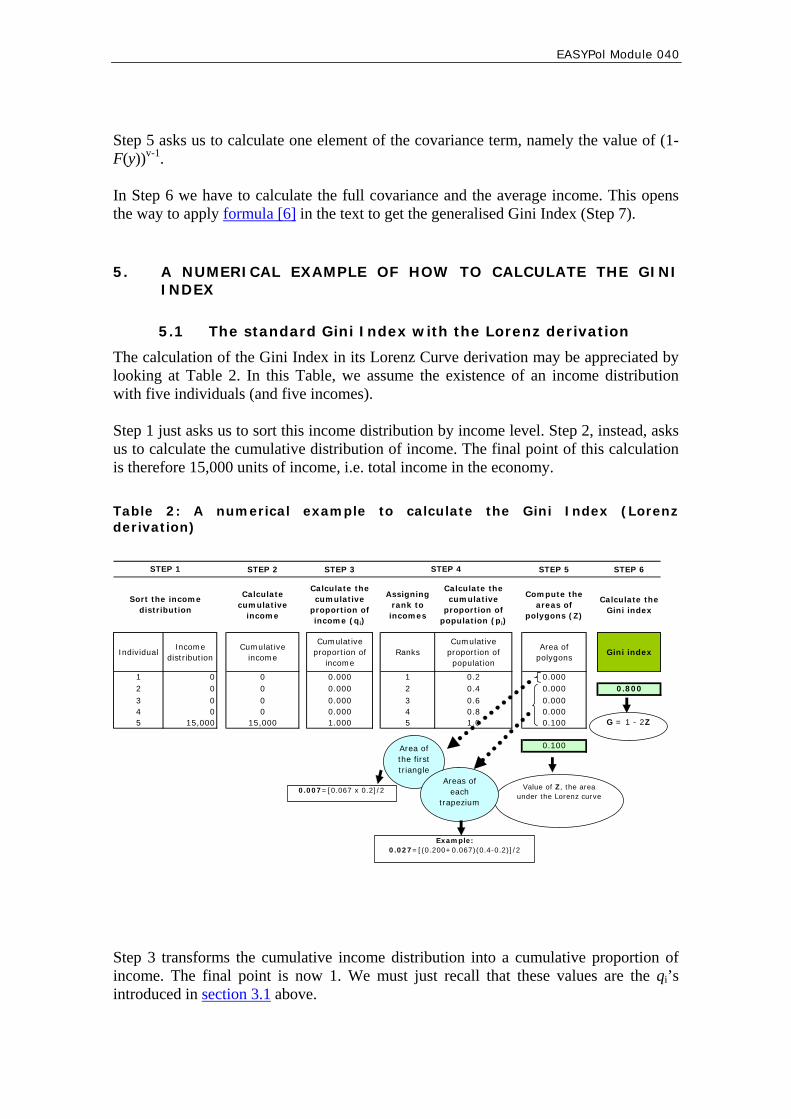
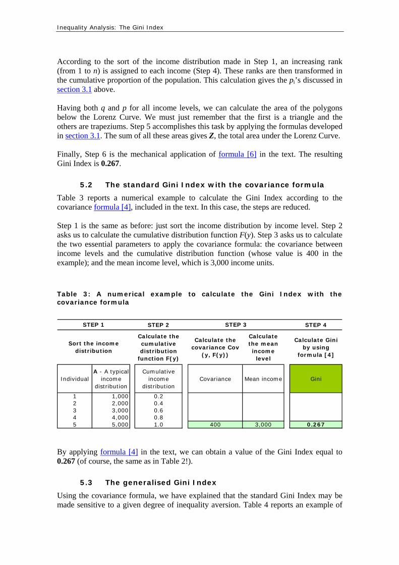
EASYPol Module 040 Analytical Tools
14
how to cope with this generalisation using the same income distribution as in Tables 2 and 3 Table 4 A numerical example to calculate the generalised Gini Index
STEP 2 STEP 3 STEP 4 STEP 5 STEP 7
Calculate the cumulative distribution
function F(y)
Calculate 1 - F(y)
Choose vCalculate
[1 - F(y)](v-1)
Calculate the covariance
Cov (y F(y))
Calculate the mean income
level
Calculate Gini by using
formula [4]
Individual
A - A typical income
distribution
Cumulative income
distribution1 - F(y) v [1 - F(y)](v-1) Covariance
Mean income
Gini
1 1000 02 08 0512 2000 04 06 0223 3000 06 04 0064 4000 08 02 0015 5000 10 00 4 000 -246 3000 0246
STEP 1 STEP 6
Sort the income distribution
Steps 1 and 2 are identical to those already discussed in Table 3 Step 3 instead asks us to calculate the values of one minus the cumulative distribution function Step 4 introduces the parameter of inequality aversion v which we have chosen to be 4 Any amount calculated in Step 3 is therefore raised at the power of (v-1) ie 3 (Step 5) Step 6 calculates the two essential parameters the covariance term (-246 in the example) and the mean income (3000) Step 7 applies formula [6] in the text giving rise to a Gini Index of 0246 Note that this value is different from that obtained with the standard Gini Index as different weights have now been attached to the same incomes
6 THE MAIN PROPERTIES OF THE GINI INDEX
This section will describe the main properties of the Gini Index in terms of the axioms it respects 8
As most of the properties are common to both the standard and the generalised Gini Index the discussion will be carried out under a common heading The main differences among the two indices will however be underlined The main properties of the Gini Index are G has zero as lower limit for any v When all incomes are equal the covariance
between income levels and the cumulative distribution function is zero The Gini Index is therefore zero With regard to the geometrical interpretation of the standard Gini Index note that when all incomes are equal the Lorenz Curve is equal to the equidistribution line Therefore the sum of areas of the polygons (Z) is equal to frac12 ie the sum of the triangle under the Lorenz Curve Therefore the Gini Index (1ndash 2Z) is equal to zero
8 See EASYPol Module 054 Policy Impacts on Inequality Inequality and Axioms for its
Measurement for a discussion of axioms in inequality measurement
Inequality Analysis The Gini Index 15
nn 1minus The standard Gini Index G has as upper limit The limit of this value for
very large populations is 1 When all incomes are zero except for the last the last income is also equal to total income y=Y It means that there is only one area to calculate ie the last trapezium However for very large populations this area tends to be smaller In the limit (ie in a continuous framework) the value of the area Z tends towards zero Therefore the Gini Index tends towards 1 As a
generalisation G(v) has n
nv
12 minus as upper limit Remember that the standard Gini
Index is one in which v=2 The Gini Index is scale invariant By multiplying all incomes by a factor α the
value of the Gini Index G does not change Intuitively when all incomes are scaled by a common factor the cumulative distribution of income does not change as a given fraction of population still holds the same fraction of total income The areas under the Lorenz Curve therefore do not change With regard to the covariance formula the application of a common factor to all incomes makes the covariance and the average income increase by the same factor The Gini Index does not change The same is true for G(v)
On the other hand the Gini Index G is not translation invariant By
addingsubtracting the same amount of money to all incomes the Gini Index would increase (decrease) accordingly The same is true for G(v)
The Gini Index satisfies the principle of transfers for any v If income is
redistributed from relatively richer individuals to relatively poorer individuals both G and G(v) decrease The opposite holds true if income is redistributed from relatively poorer to relatively richer individuals With regard to the standard Gini Index we note that the size of its change following a change in any income depends on the rank of the individuals involved in redistribution and on the sample size It does not depend on the level of individual incomes involved in redistribution but it depends on total income In particular the Gini Index reacts more to redistribution occurring among individuals who have a greater difference in ranks The same amount of redistribution indeed generates a much lower effect if the two individuals have a close rank
Table 5 illustrates how the main properties of the Gini Index work In the left panel of the table there are three simulated income distributions The first is a laquotypical oneraquo ranked by income level The second is where all individuals have the same income The third is where all individuals have zero income except for the last For the typical income distribution A the Gini Index is 0267 For the equi-distributed incomes B the Gini Index is zero while for the most concentrated income distribution
C the Gini Index is 08 ( 80541
==minusn
n )
EASYPol Module 040 Analytical Tools
16
If all incomes were increased by 20 per cent the fifth column of the table shows that the Gini Index would be unchanged (0267) This is the property of scale invariance This is not the case when all incomes are increased by the same absolute amounts (eg 2000 income units in the text) In this case Table 5 shows that the Gini Index would be lower (0160) The Gini Index is not translation invariant The Gini Index satisfies the principle of transfers If we redistribute say 500 income units from the richest to the poorest individuals the Gini Index would be lower (0213) in the text Note that the same transfers when occurring between individuals having closer ranking (the last column of Table 5) still gives rise to a lower Gini Index (0253) but higher than in the previous case (0213) This shows that the Gini Index is more sensitive to transfers occurring among individuals having distant ranks Table 5 The main properties of the Gini Index
Individual A - A typical
income distribution
B - Income distribution with equal incomes
C - Income distribution with
only one individual having income
Original income distribution with
all incomes increased by 20 per cent
Original income distribution with all incomes increased by US$ 2000
Original income distribution with a
redistribution of US$ 500 from the richest
to the poorest
Original income distribution with a
redistribution of US$ 200 from two
individuals with a close rank
1 1000 3000 0 1200 3000 1500 10002 2000 3000 0 2400 4000 2000 25003 3000 3000 0 3600 5000 3000 25004 4000 3000 0 4800 6000 4000 40005 5000 3000 15000 6000 7000 4500 5000
Total income 15000 15000 15000 18000 25000 15000 15000
GINI 0267 0000 0800 0267 0160 0213 0253
UNCHANGED DECREASED DECREASED DECREASED
The Gini index reacts less to transfersamong individuals with a close rank
7 LORENZ INTERSECTION AND THE GINI INDEX
We have explained that the Gini Index may be Lorenz-derived In other terms the Gini Index is Lorenz consistent However it is worth recalling that the ordering provided by Lorenz Curves in particular by Lorenz dominance is a partial ordering as when Lorenz Curves do not cross anything we can say which income distribution has more inequality The Gini Index instead provides for a complete ordering as it reduces the whole income distribution to a single number The basic difference between the two approaches can be appreciated by considering a case in which Lorenz Curves cross For example let us consider the two income distributions reported in Table 6 Incomes are distributed differently but the Gini Index is the same (0200)
Inequality Analysis The Gini Index 17
Table 6 Two income distributions with the same Gini Index
IndividualsIncome
distribution XIncome
distribution Y
1 2000 9002 3000 40003 4000 48004 5000 48005 6000 5500
Total income20000 20000
Gini 0200 0200 These two income distributions give rise to Lorenz Curves as depicted in Figure 7 Lorenz Curves intersect therefore they cannot be used to rank income inequality among these two income distributions But the way they intersect is such that the area before the intersection and the area after the intersection are of the same value This give rise to the same Gini Index even in the presence of quite different income distributions Figure 7 An intersection of Lorenz Curves
00
02
04
06
08
10
00 02 04 06 08 10Dis_X Dis_Y
Different income distributionsLorenz intersectionSame Gini index
Concentration areabefore intersection
Concentration areaafter intersection
EASYPol Module 040 Analytical Tools
18
8 A SYNTHESIS OF THE MAIN PROPERTIES OF THE GINI INDEX AND OF ITS GENERALISED VERSION
Table 7 gives a synthetic picture of the main properties of the Gini Index and its generalised version These properties reflect the structure of axioms 9
It is worth first noting that the lower limit of the both the standard Gini Index and of its generalised version is zero while the higher limit is differentiated The latter limit is very close to 1 (for very large populations) in the case of the standard Gini Index it tends towards 2v (again for very large populations) in the case of the generalised Gini Index Both versions of the Gini Index respect the principle of transfers However it is worth recalling that the Gini Index is more sensible for income transfers among individuals having a wide distance in their relative position (ranks) in the income distribution Both versions are scale invariant and not translation invariant and respect the principle of population This structure makes the Gini Index and the generalised version of the same index two indices belonging to the class of relative inequality indexes In applied works the characteristics of these indices are very useful hence the reason why they merit a high appeal Table 7 The Gini Index and its desirable properties
LOWER LIMIT
UPPER LIMIT
Principle of transfers
Scale invariance
Translation invariance
Principle of population
Index of relative inequality (RII)
Appeal
Gini 0 (n -1)n
YES more sensible if
individuals have distant ranks
YES NO YES YES High
Gv 0 (2v )(n -1)n
YES more sensible if
individuals have distant ranks
YES NO YES YES High
9 READERSrsquo NOTES
91 EASYPol links
Selected EASYPol modules may be used to strengthen readersrsquo background and to further expand their knowledge on inequality and inequality measurement This module belongs to a set of modules that discuss how to compare on inequality grounds alternative income distributions generated by different policy options It is part of the modules composing a training path addressing Analysis and monitoring of socio-economic impacts of policies
9 As discussed in EASYPol Module 054 Policy Impacts on Inequality Inequality and Axioms for its Measurement
Inequality Analysis The Gini Index 19
The following EASYPol modules form a set of materials logically preceding the current module which can be used to strengthen usersrsquo backgrounds
EASYPol Module 000 Charting Income Inequality The Lorenz Curve
EASYPol Module 001 Ranking Income Distribution with Lorenz Curves
EASYPol Module 007 Impacts of Policies on Poverty Basic Poverty Measures
EASYPol Module 054 Policy Impacts on Inequality Inequality and Axioms for its Measurement
Issues addressed in this module are further elaborated in the following modules
EASYPol Module 002 Social Welfare Analysis of Income Distributions Ranking Income Distribution with Generalised Lorenz Curves
EASYPol Module 041 Social Welfare Analysis of Income Distributions Social Welfare Social Welfare Functions and Inequality-Aversion
A case study presenting the use of the Gini Index to measure inequality impacts in the context an agricultural policy impact simulation exercise with real data is reported in the EASYPol Module 042 Inequality and Poverty Impacts of Selected Agricultural Policies The Case of Paraguay
EASYPol Module 040 Analytical Tools
20
10 APPENDIX I ndash ALTERNATIVE WAYS TO CALCULATE THE GINI INDEX
The geometrical derivation of the Gini Index and an alternative formula
The Lorenz derivation of the Gini Index has a direct correspondence with another rather cumbersome way to calculate the Gini Index
⎟⎠
⎞⎜⎝
⎛ ++++⎟⎠⎞
⎜⎝⎛minus+= minusminus
Yy
nY
yY
yYy
nnG nnn 121 32211 [A1]
Note the peculiarity of the last round bracket where each income share from the highest to the lowest is multiplied by the rank of individuals in the income distribution from the lowest to the highest so that the largest share has rank 1 and the smallest share has rank n This correspondence is best shown by an example with n=3 By recalling the definition of qrsquos and prsquos we get
133 1
032
031
0
0300 0
3321
3
221
2
11
1
00
0
===+++
=
=++
=
=+
=
=====
pY
yyyq
pY
yyq
pY
yq
np
Yy
q
By substituting these values into equation [2] in the text would yield
⎥⎦⎤
⎢⎣⎡ ++minus=⎥
⎦
⎤⎢⎣
⎡⎟⎠⎞
⎜⎝⎛ +
+++
+⎟⎠⎞
⎜⎝⎛ +
++minus=
Yy
Yy
Yy
Yyy
Yyyy
Yy
Yyy
YyG 123213211211
1 35
33
311
31
31
311[A2]
Let us call this definition of the Gini Index G1 Now let us also rewrite expression [A1] as
⎥⎦
⎤⎢⎣
⎡ ++minus+=Yy
Yy
Yy
G 1232 32
32
311 [A3]
Let us call this definition of the Gini Inde x G2
Inequality Analysis The Gini Index 21
Now let us rewrite [A2] and [A3] in a more convenient way by manipulating the square brackets
⎥⎦
⎤⎢⎣
⎡ +minusminus=⎥⎦
⎤⎢⎣
⎡++⎟
⎠
⎞⎜⎝
⎛ ++minus=
Yy
Yy
Yy
Yy
Yyyy
G 12121231 2
32
311
34
32
311 [A4]
⎥⎦⎤
⎢⎣⎡ +minusminus=⎥⎦
⎤⎢⎣⎡ +minusminus+=⎥
⎦
⎤⎢⎣
⎡++⎟
⎠⎞
⎜⎝⎛ ++
minus+=Yy
Yy
Yy
Yy
Yy
Yy
YyyyG 121212123
2 232
3112
32
32
3112
32
311[A5]
as the expression in round brackets in both equations is equal to 1 for n=3 It is quite easy to verify that the two expressions give the same result (G =G1 2) The formula [A1] which is often used in operational applications is therefore entirely based on the geometrical derivation of the Gini Index
101 The Gini Index with the covariance formula
In the text we have shown that the Gini Index might be directly calculated if we know the mean income and the covariance between income levels y and the cumulative distribution function F(y) Analytically
( ))(2 yFyCovy
G = [A6]
This formula is also equivalent to formula [A1] Let us see why
( )[ ] ( )[ ])(1 yFyCovyFyCov minusminus=Using the fact that since the expected value of F(y) is frac12 and the expected value of [1-F(y)] is also frac12 we can rewrite the expression [A6] as
( )[ ])(12 yFyCovy
G minusminus=
The equivalence between formula [A6] and formula [A1] can be shown again for a simplified case n=3 First of all it is worth recalling that
where E denotes the expected value (the mean) of a given variable Second it is worth defining the individual components of the covariance
( ) ( ) ( ) ( )()()( yFEyEyyFEyFyCov minus= )
( ) ( ) ( )32
333
32
31
)( 3
3
31
32
33
)(123
=++
==++
= yFEYyEyyy
yyFE
Therefore taking into account that we can yield 321 yyyY ++=
( ) [ ]13123123 9
192
92
92
91
92
93)( yyyyyyyyyFyCov minus=minusminusminus++=
EASYPol Module 040 Analytical Tools
22
nYy =By considering that the covariance formula for Gini Index becomes
[ ] ⎥⎦
⎤⎢⎣
⎡minus=minussdot
sdot=
Yy
Yy
yyY
G 1313 3
29132
Now considering that for n=3
1321 =++
Yyyy expression [A1] can be rewritten
⎥⎦
⎤⎢⎣
⎡minus=minusminusminusminusminusminus⎟
⎠
⎞⎜⎝
⎛ +++++
Yy
Yy
Yy
Yy
Yy
Yy
Yy
Yy
Yyyy
Yy
Yy
Yy 13111223321321
32
32
32
32
32
32
32
31
which is the same as that obtained with the covariance formula
102 The main properties of the Gini Index
GINI HAS ZERO AS A LOWER LIMIT We can see that for the simplified case where n=3 In the specific case Y=3y Then the formula [A1] ] would yield
034
311
36
32
311
3232
311 =minus+=⎟⎟
⎠
⎞⎜⎜⎝
⎛minus+=⎟
⎠
⎞⎜⎝
⎛ ++minus+=yy
Yy
Yy
Yy
G
GINI HAS (N-1)N AS UPPER LIMIT This can again be shown for n=3 to be Assuming again n=3 when all incomes are zero except for the last expression [3b4] would yield
nn
Yy
YYG 1
32
32
31100
32
311 minus
==minus+=⎟⎠⎞
⎜⎝⎛ ++minus+=
as in this case y=Y GINI IS SCALE INVARIANT We can see this by scaling formula [A1] by α For example with n=3 G would
become ⎟⎠⎞
⎜⎝⎛ ++minus+=⎟
⎠⎞
⎜⎝⎛
αα
+α
α+
αα
minus+=Yy
Yy
Yy
Yy
Yy
YyG 323323 32
32
31132
32
311
GINI IS NOT TRANSLATION INVARIANT This can again be seen through equation [A1] in the case of n=3 Suppose all incomes are increased by Δy = $ 2000 which means that total income will be increased by nΔy ie Equation [A1] would become 00023 sdot
Inequality Analysis The Gini Index 23
( ) ( ) ( ) ⎥⎦
⎤⎢⎣
⎡⎟⎟⎠
⎞⎜⎜⎝
⎛sdot+
++⎟⎟
⎠
⎞⎜⎜⎝
⎛sdot+
++⎟⎟
⎠
⎞⎜⎜⎝
⎛sdot+
+minus+=
000230002
3000230002
2000230002
32
311 123
Yy
Yy
Yy
G
As the numerator and the denominator of all round brackets grow in different ways their ratios are different from those of the original formula There is therefore no reason to expect the same Gini Index GINI SATISFIES THE PRINCIPLE OF TRANSFERS This can be easily seen by considering the derivative of the Gini Index with respect to the i-th income
( ) ⎟⎠⎞
⎜⎝⎛minus+⎟
⎠⎞
⎜⎝⎛minus=
partpart
Yin
nyG
i
112
rank individual43421
GINI REACTS LESS TO TRANSFERS OCCURRING AMONG INDIVIDUALS WITH CLOSER RANKS Let us explain this again by assuming n=3 and assuming first that income is redistributed from the richest person (rank 3) to the poorest person (rank 1) By totally differentiating [A1] with respect to y would yield
( ) dyY
dyY
dyY
dG ⎥⎦⎤
⎢⎣⎡minus=minus⎟
⎠⎞
⎜⎝⎛ sdotminus⎟
⎠⎞
⎜⎝⎛ sdotminus=
3411
323
32
31 y decreasing todueG ofvariation y increasing todueG ofvariation 448447648476
Now let us assume that income is redistributed from the richest individual (rank 3) to the immediately less richer individual (rank 2) In this case differentiation would yield
( ) dyY
dyY
dyY
dG ⎥⎦⎤
⎢⎣⎡minus=minus⎟
⎠⎞
⎜⎝⎛ sdotminus⎟
⎠⎞
⎜⎝⎛ sdotminus=
3211
322
32
32 y decreasing todueG ofvariation y increasing todueG ofvariation 448447648476
which is clearly lower than dG in the first case This property can be generalised by saying that given the rank of the donor (in our example from income y3) the reduction of the Gini Index is higher the more distant the rank of the receiver is from that of the donor As a consequence the Gini Index is more sensible to transfers occurring around the mode of the income distribution where there is higher density of individuals
EASYPol Module 040 Analytical Tools
24
11 REFERENCES AND FURTHER READING
Anand S 1983 Inequality and Poverty in Malaysia Oxford University Press London
UK Cowell F 1977 Measuring Inequality Phillip Allan Oxford UK Dalton H 1920 The Measurement of Inequality of Incomes Economic Journal 30 Gini C 1912 Variabilitagrave e mutabilitagrave Bologna Italy Pigou AC 1912 Wealth and Welfare MacMillan London UK Sen AK 1973 On economic Inequality Calarendon Press Oxford UK Theil H 1967 Economics and Information Theory North-Holland Amsterdam The
Netherlands Yitzhaki S 1983 On the Extension of the Gini Index International Economic Review
24 617-628
Inequality Analysis The Gini Index 25
Module metadata
1 EASYPol module 040
2 Title in original language
English Inequality Analysis
French
Spanish
Other language
3 Subtitle in original language
English The Gini Index
French
Spanish
Other language
4 Summary
This tool addresses the most popular inequality index the Gini Index It discusses its characteristics and the link with another popular graphical tool of representing inequality the Lorenz Curve Extended version of the Gini Index with different weighting schemes are also discussed The use of the Gini Index and of its generalised versions is explained through a step-by-step procedure and numerical examples
5 Date
December 2006
6 Author(s)
Lorenzo Giovanni Bellugrave Agricultural Policy Support Service Policy Assistance Division FAO Rome Italy
Paolo Liberati University of Urbino Carlo Bo Institute of Economics Urbino Italy
7 Module type Thematic overview Conceptual and technical materials
Analytical tools Applied materials Complementary resources
8 Topic covered by Agriculture in the macroeconomic context the module Agricultural and sub-sectoral policies Agro-industry and food chain policies
Environment and sustainability Institutional and organizational development Investment planning and policies Poverty and food security Regional integration and international trade Rural Development
9 Subtopics covered by the module
10 Training path Analysis and monitoring of socio-economic impacts of policies
EASYPol Module 040 Analytical Tools
26
11 Keywords capacity building agriculture agricultural policies agricultural development development policies policy analysis policy impact anlaysis poverty food security analytical tool inequality inequality analysis inequality index inequality measures cost-benefit analysis gini index generalised gini index lorenz curve social welfare analysis

EASYPol Module 040 Analytical Tools
16
If all incomes were increased by 20 per cent the fifth column of the table shows that the Gini Index would be unchanged (0267) This is the property of scale invariance This is not the case when all incomes are increased by the same absolute amounts (eg 2000 income units in the text) In this case Table 5 shows that the Gini Index would be lower (0160) The Gini Index is not translation invariant The Gini Index satisfies the principle of transfers If we redistribute say 500 income units from the richest to the poorest individuals the Gini Index would be lower (0213) in the text Note that the same transfers when occurring between individuals having closer ranking (the last column of Table 5) still gives rise to a lower Gini Index (0253) but higher than in the previous case (0213) This shows that the Gini Index is more sensitive to transfers occurring among individuals having distant ranks Table 5 The main properties of the Gini Index
Individual A - A typical
income distribution
B - Income distribution with equal incomes
C - Income distribution with
only one individual having income
Original income distribution with
all incomes increased by 20 per cent
Original income distribution with all incomes increased by US$ 2000
Original income distribution with a
redistribution of US$ 500 from the richest
to the poorest
Original income distribution with a
redistribution of US$ 200 from two
individuals with a close rank
1 1000 3000 0 1200 3000 1500 10002 2000 3000 0 2400 4000 2000 25003 3000 3000 0 3600 5000 3000 25004 4000 3000 0 4800 6000 4000 40005 5000 3000 15000 6000 7000 4500 5000
Total income 15000 15000 15000 18000 25000 15000 15000
GINI 0267 0000 0800 0267 0160 0213 0253
UNCHANGED DECREASED DECREASED DECREASED
The Gini index reacts less to transfersamong individuals with a close rank
7 LORENZ INTERSECTION AND THE GINI INDEX
We have explained that the Gini Index may be Lorenz-derived In other terms the Gini Index is Lorenz consistent However it is worth recalling that the ordering provided by Lorenz Curves in particular by Lorenz dominance is a partial ordering as when Lorenz Curves do not cross anything we can say which income distribution has more inequality The Gini Index instead provides for a complete ordering as it reduces the whole income distribution to a single number The basic difference between the two approaches can be appreciated by considering a case in which Lorenz Curves cross For example let us consider the two income distributions reported in Table 6 Incomes are distributed differently but the Gini Index is the same (0200)
Inequality Analysis The Gini Index 17
Table 6 Two income distributions with the same Gini Index
IndividualsIncome
distribution XIncome
distribution Y
1 2000 9002 3000 40003 4000 48004 5000 48005 6000 5500
Total income20000 20000
Gini 0200 0200 These two income distributions give rise to Lorenz Curves as depicted in Figure 7 Lorenz Curves intersect therefore they cannot be used to rank income inequality among these two income distributions But the way they intersect is such that the area before the intersection and the area after the intersection are of the same value This give rise to the same Gini Index even in the presence of quite different income distributions Figure 7 An intersection of Lorenz Curves
00
02
04
06
08
10
00 02 04 06 08 10Dis_X Dis_Y
Different income distributionsLorenz intersectionSame Gini index
Concentration areabefore intersection
Concentration areaafter intersection
EASYPol Module 040 Analytical Tools
18
8 A SYNTHESIS OF THE MAIN PROPERTIES OF THE GINI INDEX AND OF ITS GENERALISED VERSION
Table 7 gives a synthetic picture of the main properties of the Gini Index and its generalised version These properties reflect the structure of axioms 9
It is worth first noting that the lower limit of the both the standard Gini Index and of its generalised version is zero while the higher limit is differentiated The latter limit is very close to 1 (for very large populations) in the case of the standard Gini Index it tends towards 2v (again for very large populations) in the case of the generalised Gini Index Both versions of the Gini Index respect the principle of transfers However it is worth recalling that the Gini Index is more sensible for income transfers among individuals having a wide distance in their relative position (ranks) in the income distribution Both versions are scale invariant and not translation invariant and respect the principle of population This structure makes the Gini Index and the generalised version of the same index two indices belonging to the class of relative inequality indexes In applied works the characteristics of these indices are very useful hence the reason why they merit a high appeal Table 7 The Gini Index and its desirable properties
LOWER LIMIT
UPPER LIMIT
Principle of transfers
Scale invariance
Translation invariance
Principle of population
Index of relative inequality (RII)
Appeal
Gini 0 (n -1)n
YES more sensible if
individuals have distant ranks
YES NO YES YES High
Gv 0 (2v )(n -1)n
YES more sensible if
individuals have distant ranks
YES NO YES YES High
9 READERSrsquo NOTES
91 EASYPol links
Selected EASYPol modules may be used to strengthen readersrsquo background and to further expand their knowledge on inequality and inequality measurement This module belongs to a set of modules that discuss how to compare on inequality grounds alternative income distributions generated by different policy options It is part of the modules composing a training path addressing Analysis and monitoring of socio-economic impacts of policies
9 As discussed in EASYPol Module 054 Policy Impacts on Inequality Inequality and Axioms for its Measurement
Inequality Analysis The Gini Index 19
The following EASYPol modules form a set of materials logically preceding the current module which can be used to strengthen usersrsquo backgrounds
EASYPol Module 000 Charting Income Inequality The Lorenz Curve
EASYPol Module 001 Ranking Income Distribution with Lorenz Curves
EASYPol Module 007 Impacts of Policies on Poverty Basic Poverty Measures
EASYPol Module 054 Policy Impacts on Inequality Inequality and Axioms for its Measurement
Issues addressed in this module are further elaborated in the following modules
EASYPol Module 002 Social Welfare Analysis of Income Distributions Ranking Income Distribution with Generalised Lorenz Curves
EASYPol Module 041 Social Welfare Analysis of Income Distributions Social Welfare Social Welfare Functions and Inequality-Aversion
A case study presenting the use of the Gini Index to measure inequality impacts in the context an agricultural policy impact simulation exercise with real data is reported in the EASYPol Module 042 Inequality and Poverty Impacts of Selected Agricultural Policies The Case of Paraguay
EASYPol Module 040 Analytical Tools
20
10 APPENDIX I ndash ALTERNATIVE WAYS TO CALCULATE THE GINI INDEX
The geometrical derivation of the Gini Index and an alternative formula
The Lorenz derivation of the Gini Index has a direct correspondence with another rather cumbersome way to calculate the Gini Index
⎟⎠
⎞⎜⎝
⎛ ++++⎟⎠⎞
⎜⎝⎛minus+= minusminus
Yy
nY
yY
yYy
nnG nnn 121 32211 [A1]
Note the peculiarity of the last round bracket where each income share from the highest to the lowest is multiplied by the rank of individuals in the income distribution from the lowest to the highest so that the largest share has rank 1 and the smallest share has rank n This correspondence is best shown by an example with n=3 By recalling the definition of qrsquos and prsquos we get
133 1
032
031
0
0300 0
3321
3
221
2
11
1
00
0
===+++
=
=++
=
=+
=
=====
pY
yyyq
pY
yyq
pY
yq
np
Yy
q
By substituting these values into equation [2] in the text would yield
⎥⎦⎤
⎢⎣⎡ ++minus=⎥
⎦
⎤⎢⎣
⎡⎟⎠⎞
⎜⎝⎛ +
+++
+⎟⎠⎞
⎜⎝⎛ +
++minus=
Yy
Yy
Yy
Yyy
Yyyy
Yy
Yyy
YyG 123213211211
1 35
33
311
31
31
311[A2]
Let us call this definition of the Gini Index G1 Now let us also rewrite expression [A1] as
⎥⎦
⎤⎢⎣
⎡ ++minus+=Yy
Yy
Yy
G 1232 32
32
311 [A3]
Let us call this definition of the Gini Inde x G2
Inequality Analysis The Gini Index 21
Now let us rewrite [A2] and [A3] in a more convenient way by manipulating the square brackets
⎥⎦
⎤⎢⎣
⎡ +minusminus=⎥⎦
⎤⎢⎣
⎡++⎟
⎠
⎞⎜⎝
⎛ ++minus=
Yy
Yy
Yy
Yy
Yyyy
G 12121231 2
32
311
34
32
311 [A4]
⎥⎦⎤
⎢⎣⎡ +minusminus=⎥⎦
⎤⎢⎣⎡ +minusminus+=⎥
⎦
⎤⎢⎣
⎡++⎟
⎠⎞
⎜⎝⎛ ++
minus+=Yy
Yy
Yy
Yy
Yy
Yy
YyyyG 121212123
2 232
3112
32
32
3112
32
311[A5]
as the expression in round brackets in both equations is equal to 1 for n=3 It is quite easy to verify that the two expressions give the same result (G =G1 2) The formula [A1] which is often used in operational applications is therefore entirely based on the geometrical derivation of the Gini Index
101 The Gini Index with the covariance formula
In the text we have shown that the Gini Index might be directly calculated if we know the mean income and the covariance between income levels y and the cumulative distribution function F(y) Analytically
( ))(2 yFyCovy
G = [A6]
This formula is also equivalent to formula [A1] Let us see why
( )[ ] ( )[ ])(1 yFyCovyFyCov minusminus=Using the fact that since the expected value of F(y) is frac12 and the expected value of [1-F(y)] is also frac12 we can rewrite the expression [A6] as
( )[ ])(12 yFyCovy
G minusminus=
The equivalence between formula [A6] and formula [A1] can be shown again for a simplified case n=3 First of all it is worth recalling that
where E denotes the expected value (the mean) of a given variable Second it is worth defining the individual components of the covariance
( ) ( ) ( ) ( )()()( yFEyEyyFEyFyCov minus= )
( ) ( ) ( )32
333
32
31
)( 3
3
31
32
33
)(123
=++
==++
= yFEYyEyyy
yyFE
Therefore taking into account that we can yield 321 yyyY ++=
( ) [ ]13123123 9
192
92
92
91
92
93)( yyyyyyyyyFyCov minus=minusminusminus++=
EASYPol Module 040 Analytical Tools
22
nYy =By considering that the covariance formula for Gini Index becomes
[ ] ⎥⎦
⎤⎢⎣
⎡minus=minussdot
sdot=
Yy
Yy
yyY
G 1313 3
29132
Now considering that for n=3
1321 =++
Yyyy expression [A1] can be rewritten
⎥⎦
⎤⎢⎣
⎡minus=minusminusminusminusminusminus⎟
⎠
⎞⎜⎝
⎛ +++++
Yy
Yy
Yy
Yy
Yy
Yy
Yy
Yy
Yyyy
Yy
Yy
Yy 13111223321321
32
32
32
32
32
32
32
31
which is the same as that obtained with the covariance formula
102 The main properties of the Gini Index
GINI HAS ZERO AS A LOWER LIMIT We can see that for the simplified case where n=3 In the specific case Y=3y Then the formula [A1] ] would yield
034
311
36
32
311
3232
311 =minus+=⎟⎟
⎠
⎞⎜⎜⎝
⎛minus+=⎟
⎠
⎞⎜⎝
⎛ ++minus+=yy
Yy
Yy
Yy
G
GINI HAS (N-1)N AS UPPER LIMIT This can again be shown for n=3 to be Assuming again n=3 when all incomes are zero except for the last expression [3b4] would yield
nn
Yy
YYG 1
32
32
31100
32
311 minus
==minus+=⎟⎠⎞
⎜⎝⎛ ++minus+=
as in this case y=Y GINI IS SCALE INVARIANT We can see this by scaling formula [A1] by α For example with n=3 G would
become ⎟⎠⎞
⎜⎝⎛ ++minus+=⎟
⎠⎞
⎜⎝⎛
αα
+α
α+
αα
minus+=Yy
Yy
Yy
Yy
Yy
YyG 323323 32
32
31132
32
311
GINI IS NOT TRANSLATION INVARIANT This can again be seen through equation [A1] in the case of n=3 Suppose all incomes are increased by Δy = $ 2000 which means that total income will be increased by nΔy ie Equation [A1] would become 00023 sdot
Inequality Analysis The Gini Index 23
( ) ( ) ( ) ⎥⎦
⎤⎢⎣
⎡⎟⎟⎠
⎞⎜⎜⎝
⎛sdot+
++⎟⎟
⎠
⎞⎜⎜⎝
⎛sdot+
++⎟⎟
⎠
⎞⎜⎜⎝
⎛sdot+
+minus+=
000230002
3000230002
2000230002
32
311 123
Yy
Yy
Yy
G
As the numerator and the denominator of all round brackets grow in different ways their ratios are different from those of the original formula There is therefore no reason to expect the same Gini Index GINI SATISFIES THE PRINCIPLE OF TRANSFERS This can be easily seen by considering the derivative of the Gini Index with respect to the i-th income
( ) ⎟⎠⎞
⎜⎝⎛minus+⎟
⎠⎞
⎜⎝⎛minus=
partpart
Yin
nyG
i
112
rank individual43421
GINI REACTS LESS TO TRANSFERS OCCURRING AMONG INDIVIDUALS WITH CLOSER RANKS Let us explain this again by assuming n=3 and assuming first that income is redistributed from the richest person (rank 3) to the poorest person (rank 1) By totally differentiating [A1] with respect to y would yield
( ) dyY
dyY
dyY
dG ⎥⎦⎤
⎢⎣⎡minus=minus⎟
⎠⎞
⎜⎝⎛ sdotminus⎟
⎠⎞
⎜⎝⎛ sdotminus=
3411
323
32
31 y decreasing todueG ofvariation y increasing todueG ofvariation 448447648476
Now let us assume that income is redistributed from the richest individual (rank 3) to the immediately less richer individual (rank 2) In this case differentiation would yield
( ) dyY
dyY
dyY
dG ⎥⎦⎤
⎢⎣⎡minus=minus⎟
⎠⎞
⎜⎝⎛ sdotminus⎟
⎠⎞
⎜⎝⎛ sdotminus=
3211
322
32
32 y decreasing todueG ofvariation y increasing todueG ofvariation 448447648476
which is clearly lower than dG in the first case This property can be generalised by saying that given the rank of the donor (in our example from income y3) the reduction of the Gini Index is higher the more distant the rank of the receiver is from that of the donor As a consequence the Gini Index is more sensible to transfers occurring around the mode of the income distribution where there is higher density of individuals
EASYPol Module 040 Analytical Tools
24
11 REFERENCES AND FURTHER READING
Anand S 1983 Inequality and Poverty in Malaysia Oxford University Press London
UK Cowell F 1977 Measuring Inequality Phillip Allan Oxford UK Dalton H 1920 The Measurement of Inequality of Incomes Economic Journal 30 Gini C 1912 Variabilitagrave e mutabilitagrave Bologna Italy Pigou AC 1912 Wealth and Welfare MacMillan London UK Sen AK 1973 On economic Inequality Calarendon Press Oxford UK Theil H 1967 Economics and Information Theory North-Holland Amsterdam The
Netherlands Yitzhaki S 1983 On the Extension of the Gini Index International Economic Review
24 617-628
Inequality Analysis The Gini Index 25
Module metadata
1 EASYPol module 040
2 Title in original language
English Inequality Analysis
French
Spanish
Other language
3 Subtitle in original language
English The Gini Index
French
Spanish
Other language
4 Summary
This tool addresses the most popular inequality index the Gini Index It discusses its characteristics and the link with another popular graphical tool of representing inequality the Lorenz Curve Extended version of the Gini Index with different weighting schemes are also discussed The use of the Gini Index and of its generalised versions is explained through a step-by-step procedure and numerical examples
5 Date
December 2006
6 Author(s)
Lorenzo Giovanni Bellugrave Agricultural Policy Support Service Policy Assistance Division FAO Rome Italy
Paolo Liberati University of Urbino Carlo Bo Institute of Economics Urbino Italy
7 Module type Thematic overview Conceptual and technical materials
Analytical tools Applied materials Complementary resources
8 Topic covered by Agriculture in the macroeconomic context the module Agricultural and sub-sectoral policies Agro-industry and food chain policies
Environment and sustainability Institutional and organizational development Investment planning and policies Poverty and food security Regional integration and international trade Rural Development
9 Subtopics covered by the module
10 Training path Analysis and monitoring of socio-economic impacts of policies
EASYPol Module 040 Analytical Tools
26
11 Keywords capacity building agriculture agricultural policies agricultural development development policies policy analysis policy impact anlaysis poverty food security analytical tool inequality inequality analysis inequality index inequality measures cost-benefit analysis gini index generalised gini index lorenz curve social welfare analysis
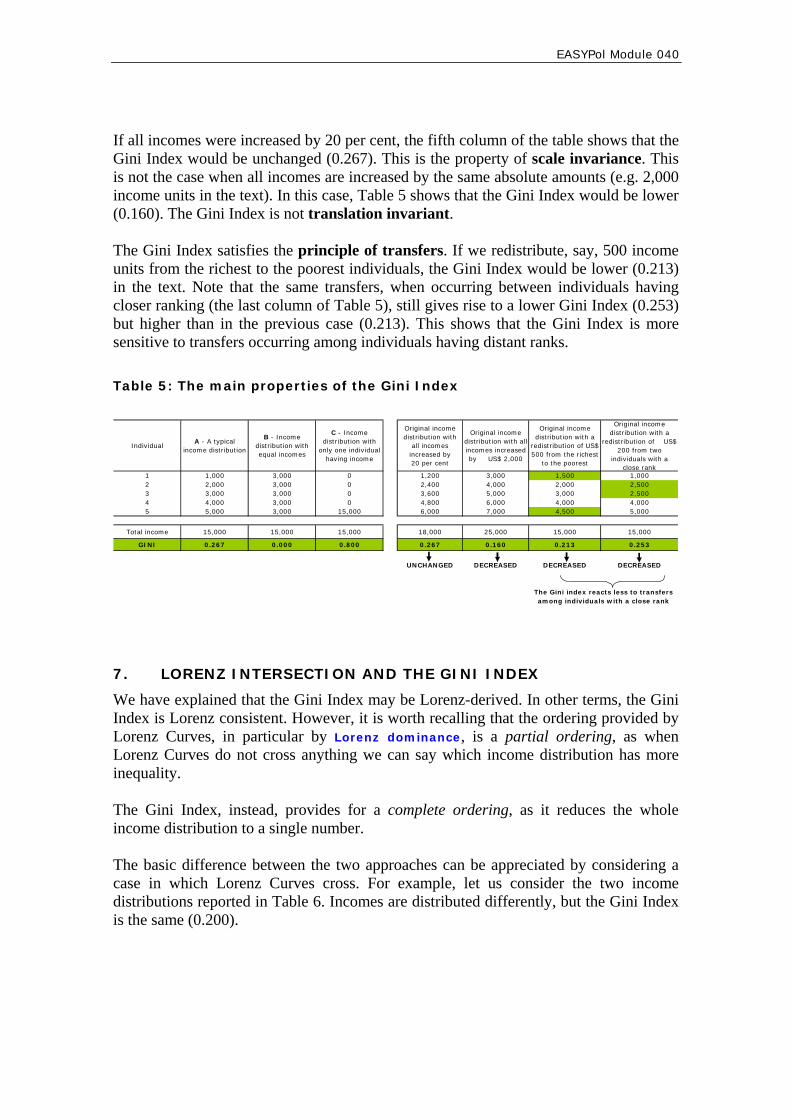
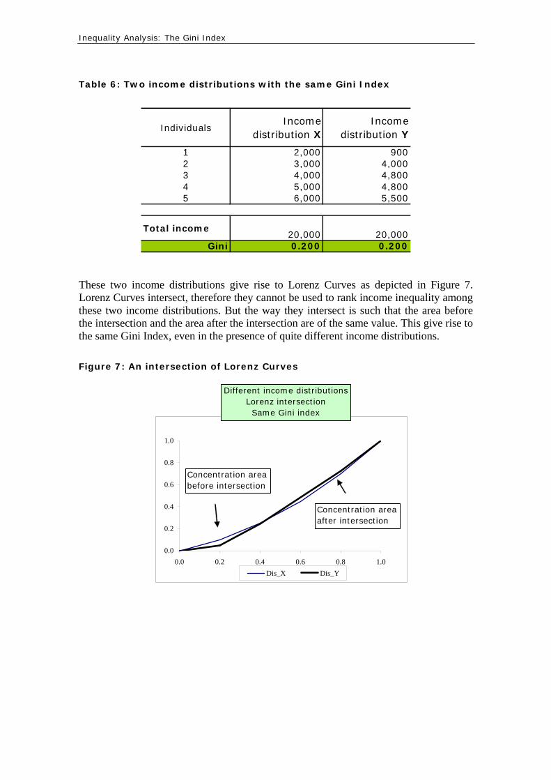
EASYPol Module 040 Analytical Tools
18
8 A SYNTHESIS OF THE MAIN PROPERTIES OF THE GINI INDEX AND OF ITS GENERALISED VERSION
Table 7 gives a synthetic picture of the main properties of the Gini Index and its generalised version These properties reflect the structure of axioms 9
It is worth first noting that the lower limit of the both the standard Gini Index and of its generalised version is zero while the higher limit is differentiated The latter limit is very close to 1 (for very large populations) in the case of the standard Gini Index it tends towards 2v (again for very large populations) in the case of the generalised Gini Index Both versions of the Gini Index respect the principle of transfers However it is worth recalling that the Gini Index is more sensible for income transfers among individuals having a wide distance in their relative position (ranks) in the income distribution Both versions are scale invariant and not translation invariant and respect the principle of population This structure makes the Gini Index and the generalised version of the same index two indices belonging to the class of relative inequality indexes In applied works the characteristics of these indices are very useful hence the reason why they merit a high appeal Table 7 The Gini Index and its desirable properties
LOWER LIMIT
UPPER LIMIT
Principle of transfers
Scale invariance
Translation invariance
Principle of population
Index of relative inequality (RII)
Appeal
Gini 0 (n -1)n
YES more sensible if
individuals have distant ranks
YES NO YES YES High
Gv 0 (2v )(n -1)n
YES more sensible if
individuals have distant ranks
YES NO YES YES High
9 READERSrsquo NOTES
91 EASYPol links
Selected EASYPol modules may be used to strengthen readersrsquo background and to further expand their knowledge on inequality and inequality measurement This module belongs to a set of modules that discuss how to compare on inequality grounds alternative income distributions generated by different policy options It is part of the modules composing a training path addressing Analysis and monitoring of socio-economic impacts of policies
9 As discussed in EASYPol Module 054 Policy Impacts on Inequality Inequality and Axioms for its Measurement
Inequality Analysis The Gini Index 19
The following EASYPol modules form a set of materials logically preceding the current module which can be used to strengthen usersrsquo backgrounds
EASYPol Module 000 Charting Income Inequality The Lorenz Curve
EASYPol Module 001 Ranking Income Distribution with Lorenz Curves
EASYPol Module 007 Impacts of Policies on Poverty Basic Poverty Measures
EASYPol Module 054 Policy Impacts on Inequality Inequality and Axioms for its Measurement
Issues addressed in this module are further elaborated in the following modules
EASYPol Module 002 Social Welfare Analysis of Income Distributions Ranking Income Distribution with Generalised Lorenz Curves
EASYPol Module 041 Social Welfare Analysis of Income Distributions Social Welfare Social Welfare Functions and Inequality-Aversion
A case study presenting the use of the Gini Index to measure inequality impacts in the context an agricultural policy impact simulation exercise with real data is reported in the EASYPol Module 042 Inequality and Poverty Impacts of Selected Agricultural Policies The Case of Paraguay
EASYPol Module 040 Analytical Tools
20
10 APPENDIX I ndash ALTERNATIVE WAYS TO CALCULATE THE GINI INDEX
The geometrical derivation of the Gini Index and an alternative formula
The Lorenz derivation of the Gini Index has a direct correspondence with another rather cumbersome way to calculate the Gini Index
⎟⎠
⎞⎜⎝
⎛ ++++⎟⎠⎞
⎜⎝⎛minus+= minusminus
Yy
nY
yY
yYy
nnG nnn 121 32211 [A1]
Note the peculiarity of the last round bracket where each income share from the highest to the lowest is multiplied by the rank of individuals in the income distribution from the lowest to the highest so that the largest share has rank 1 and the smallest share has rank n This correspondence is best shown by an example with n=3 By recalling the definition of qrsquos and prsquos we get
133 1
032
031
0
0300 0
3321
3
221
2
11
1
00
0
===+++
=
=++
=
=+
=
=====
pY
yyyq
pY
yyq
pY
yq
np
Yy
q
By substituting these values into equation [2] in the text would yield
⎥⎦⎤
⎢⎣⎡ ++minus=⎥
⎦
⎤⎢⎣
⎡⎟⎠⎞
⎜⎝⎛ +
+++
+⎟⎠⎞
⎜⎝⎛ +
++minus=
Yy
Yy
Yy
Yyy
Yyyy
Yy
Yyy
YyG 123213211211
1 35
33
311
31
31
311[A2]
Let us call this definition of the Gini Index G1 Now let us also rewrite expression [A1] as
⎥⎦
⎤⎢⎣
⎡ ++minus+=Yy
Yy
Yy
G 1232 32
32
311 [A3]
Let us call this definition of the Gini Inde x G2
Inequality Analysis The Gini Index 21
Now let us rewrite [A2] and [A3] in a more convenient way by manipulating the square brackets
⎥⎦
⎤⎢⎣
⎡ +minusminus=⎥⎦
⎤⎢⎣
⎡++⎟
⎠
⎞⎜⎝
⎛ ++minus=
Yy
Yy
Yy
Yy
Yyyy
G 12121231 2
32
311
34
32
311 [A4]
⎥⎦⎤
⎢⎣⎡ +minusminus=⎥⎦
⎤⎢⎣⎡ +minusminus+=⎥
⎦
⎤⎢⎣
⎡++⎟
⎠⎞
⎜⎝⎛ ++
minus+=Yy
Yy
Yy
Yy
Yy
Yy
YyyyG 121212123
2 232
3112
32
32
3112
32
311[A5]
as the expression in round brackets in both equations is equal to 1 for n=3 It is quite easy to verify that the two expressions give the same result (G =G1 2) The formula [A1] which is often used in operational applications is therefore entirely based on the geometrical derivation of the Gini Index
101 The Gini Index with the covariance formula
In the text we have shown that the Gini Index might be directly calculated if we know the mean income and the covariance between income levels y and the cumulative distribution function F(y) Analytically
( ))(2 yFyCovy
G = [A6]
This formula is also equivalent to formula [A1] Let us see why
( )[ ] ( )[ ])(1 yFyCovyFyCov minusminus=Using the fact that since the expected value of F(y) is frac12 and the expected value of [1-F(y)] is also frac12 we can rewrite the expression [A6] as
( )[ ])(12 yFyCovy
G minusminus=
The equivalence between formula [A6] and formula [A1] can be shown again for a simplified case n=3 First of all it is worth recalling that
where E denotes the expected value (the mean) of a given variable Second it is worth defining the individual components of the covariance
( ) ( ) ( ) ( )()()( yFEyEyyFEyFyCov minus= )
( ) ( ) ( )32
333
32
31
)( 3
3
31
32
33
)(123
=++
==++
= yFEYyEyyy
yyFE
Therefore taking into account that we can yield 321 yyyY ++=
( ) [ ]13123123 9
192
92
92
91
92
93)( yyyyyyyyyFyCov minus=minusminusminus++=
EASYPol Module 040 Analytical Tools
22
nYy =By considering that the covariance formula for Gini Index becomes
[ ] ⎥⎦
⎤⎢⎣
⎡minus=minussdot
sdot=
Yy
Yy
yyY
G 1313 3
29132
Now considering that for n=3
1321 =++
Yyyy expression [A1] can be rewritten
⎥⎦
⎤⎢⎣
⎡minus=minusminusminusminusminusminus⎟
⎠
⎞⎜⎝
⎛ +++++
Yy
Yy
Yy
Yy
Yy
Yy
Yy
Yy
Yyyy
Yy
Yy
Yy 13111223321321
32
32
32
32
32
32
32
31
which is the same as that obtained with the covariance formula
102 The main properties of the Gini Index
GINI HAS ZERO AS A LOWER LIMIT We can see that for the simplified case where n=3 In the specific case Y=3y Then the formula [A1] ] would yield
034
311
36
32
311
3232
311 =minus+=⎟⎟
⎠
⎞⎜⎜⎝
⎛minus+=⎟
⎠
⎞⎜⎝
⎛ ++minus+=yy
Yy
Yy
Yy
G
GINI HAS (N-1)N AS UPPER LIMIT This can again be shown for n=3 to be Assuming again n=3 when all incomes are zero except for the last expression [3b4] would yield
nn
Yy
YYG 1
32
32
31100
32
311 minus
==minus+=⎟⎠⎞
⎜⎝⎛ ++minus+=
as in this case y=Y GINI IS SCALE INVARIANT We can see this by scaling formula [A1] by α For example with n=3 G would
become ⎟⎠⎞
⎜⎝⎛ ++minus+=⎟
⎠⎞
⎜⎝⎛
αα
+α
α+
αα
minus+=Yy
Yy
Yy
Yy
Yy
YyG 323323 32
32
31132
32
311
GINI IS NOT TRANSLATION INVARIANT This can again be seen through equation [A1] in the case of n=3 Suppose all incomes are increased by Δy = $ 2000 which means that total income will be increased by nΔy ie Equation [A1] would become 00023 sdot
Inequality Analysis The Gini Index 23
( ) ( ) ( ) ⎥⎦
⎤⎢⎣
⎡⎟⎟⎠
⎞⎜⎜⎝
⎛sdot+
++⎟⎟
⎠
⎞⎜⎜⎝
⎛sdot+
++⎟⎟
⎠
⎞⎜⎜⎝
⎛sdot+
+minus+=
000230002
3000230002
2000230002
32
311 123
Yy
Yy
Yy
G
As the numerator and the denominator of all round brackets grow in different ways their ratios are different from those of the original formula There is therefore no reason to expect the same Gini Index GINI SATISFIES THE PRINCIPLE OF TRANSFERS This can be easily seen by considering the derivative of the Gini Index with respect to the i-th income
( ) ⎟⎠⎞
⎜⎝⎛minus+⎟
⎠⎞
⎜⎝⎛minus=
partpart
Yin
nyG
i
112
rank individual43421
GINI REACTS LESS TO TRANSFERS OCCURRING AMONG INDIVIDUALS WITH CLOSER RANKS Let us explain this again by assuming n=3 and assuming first that income is redistributed from the richest person (rank 3) to the poorest person (rank 1) By totally differentiating [A1] with respect to y would yield
( ) dyY
dyY
dyY
dG ⎥⎦⎤
⎢⎣⎡minus=minus⎟
⎠⎞
⎜⎝⎛ sdotminus⎟
⎠⎞
⎜⎝⎛ sdotminus=
3411
323
32
31 y decreasing todueG ofvariation y increasing todueG ofvariation 448447648476
Now let us assume that income is redistributed from the richest individual (rank 3) to the immediately less richer individual (rank 2) In this case differentiation would yield
( ) dyY
dyY
dyY
dG ⎥⎦⎤
⎢⎣⎡minus=minus⎟
⎠⎞
⎜⎝⎛ sdotminus⎟
⎠⎞
⎜⎝⎛ sdotminus=
3211
322
32
32 y decreasing todueG ofvariation y increasing todueG ofvariation 448447648476
which is clearly lower than dG in the first case This property can be generalised by saying that given the rank of the donor (in our example from income y3) the reduction of the Gini Index is higher the more distant the rank of the receiver is from that of the donor As a consequence the Gini Index is more sensible to transfers occurring around the mode of the income distribution where there is higher density of individuals
EASYPol Module 040 Analytical Tools
24
11 REFERENCES AND FURTHER READING
Anand S 1983 Inequality and Poverty in Malaysia Oxford University Press London
UK Cowell F 1977 Measuring Inequality Phillip Allan Oxford UK Dalton H 1920 The Measurement of Inequality of Incomes Economic Journal 30 Gini C 1912 Variabilitagrave e mutabilitagrave Bologna Italy Pigou AC 1912 Wealth and Welfare MacMillan London UK Sen AK 1973 On economic Inequality Calarendon Press Oxford UK Theil H 1967 Economics and Information Theory North-Holland Amsterdam The
Netherlands Yitzhaki S 1983 On the Extension of the Gini Index International Economic Review
24 617-628
Inequality Analysis The Gini Index 25
Module metadata
1 EASYPol module 040
2 Title in original language
English Inequality Analysis
French
Spanish
Other language
3 Subtitle in original language
English The Gini Index
French
Spanish
Other language
4 Summary
This tool addresses the most popular inequality index the Gini Index It discusses its characteristics and the link with another popular graphical tool of representing inequality the Lorenz Curve Extended version of the Gini Index with different weighting schemes are also discussed The use of the Gini Index and of its generalised versions is explained through a step-by-step procedure and numerical examples
5 Date
December 2006
6 Author(s)
Lorenzo Giovanni Bellugrave Agricultural Policy Support Service Policy Assistance Division FAO Rome Italy
Paolo Liberati University of Urbino Carlo Bo Institute of Economics Urbino Italy
7 Module type Thematic overview Conceptual and technical materials
Analytical tools Applied materials Complementary resources
8 Topic covered by Agriculture in the macroeconomic context the module Agricultural and sub-sectoral policies Agro-industry and food chain policies
Environment and sustainability Institutional and organizational development Investment planning and policies Poverty and food security Regional integration and international trade Rural Development
9 Subtopics covered by the module
10 Training path Analysis and monitoring of socio-economic impacts of policies
EASYPol Module 040 Analytical Tools
26
11 Keywords capacity building agriculture agricultural policies agricultural development development policies policy analysis policy impact anlaysis poverty food security analytical tool inequality inequality analysis inequality index inequality measures cost-benefit analysis gini index generalised gini index lorenz curve social welfare analysis
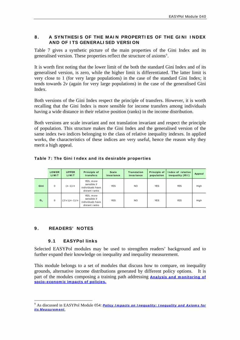

EASYPol Module 040 Analytical Tools
20
10 APPENDIX I ndash ALTERNATIVE WAYS TO CALCULATE THE GINI INDEX
The geometrical derivation of the Gini Index and an alternative formula
The Lorenz derivation of the Gini Index has a direct correspondence with another rather cumbersome way to calculate the Gini Index
⎟⎠
⎞⎜⎝
⎛ ++++⎟⎠⎞
⎜⎝⎛minus+= minusminus
Yy
nY
yY
yYy
nnG nnn 121 32211 [A1]
Note the peculiarity of the last round bracket where each income share from the highest to the lowest is multiplied by the rank of individuals in the income distribution from the lowest to the highest so that the largest share has rank 1 and the smallest share has rank n This correspondence is best shown by an example with n=3 By recalling the definition of qrsquos and prsquos we get
133 1
032
031
0
0300 0
3321
3
221
2
11
1
00
0
===+++
=
=++
=
=+
=
=====
pY
yyyq
pY
yyq
pY
yq
np
Yy
q
By substituting these values into equation [2] in the text would yield
⎥⎦⎤
⎢⎣⎡ ++minus=⎥
⎦
⎤⎢⎣
⎡⎟⎠⎞
⎜⎝⎛ +
+++
+⎟⎠⎞
⎜⎝⎛ +
++minus=
Yy
Yy
Yy
Yyy
Yyyy
Yy
Yyy
YyG 123213211211
1 35
33
311
31
31
311[A2]
Let us call this definition of the Gini Index G1 Now let us also rewrite expression [A1] as
⎥⎦
⎤⎢⎣
⎡ ++minus+=Yy
Yy
Yy
G 1232 32
32
311 [A3]
Let us call this definition of the Gini Inde x G2
Inequality Analysis The Gini Index 21
Now let us rewrite [A2] and [A3] in a more convenient way by manipulating the square brackets
⎥⎦
⎤⎢⎣
⎡ +minusminus=⎥⎦
⎤⎢⎣
⎡++⎟
⎠
⎞⎜⎝
⎛ ++minus=
Yy
Yy
Yy
Yy
Yyyy
G 12121231 2
32
311
34
32
311 [A4]
⎥⎦⎤
⎢⎣⎡ +minusminus=⎥⎦
⎤⎢⎣⎡ +minusminus+=⎥
⎦
⎤⎢⎣
⎡++⎟
⎠⎞
⎜⎝⎛ ++
minus+=Yy
Yy
Yy
Yy
Yy
Yy
YyyyG 121212123
2 232
3112
32
32
3112
32
311[A5]
as the expression in round brackets in both equations is equal to 1 for n=3 It is quite easy to verify that the two expressions give the same result (G =G1 2) The formula [A1] which is often used in operational applications is therefore entirely based on the geometrical derivation of the Gini Index
101 The Gini Index with the covariance formula
In the text we have shown that the Gini Index might be directly calculated if we know the mean income and the covariance between income levels y and the cumulative distribution function F(y) Analytically
( ))(2 yFyCovy
G = [A6]
This formula is also equivalent to formula [A1] Let us see why
( )[ ] ( )[ ])(1 yFyCovyFyCov minusminus=Using the fact that since the expected value of F(y) is frac12 and the expected value of [1-F(y)] is also frac12 we can rewrite the expression [A6] as
( )[ ])(12 yFyCovy
G minusminus=
The equivalence between formula [A6] and formula [A1] can be shown again for a simplified case n=3 First of all it is worth recalling that
where E denotes the expected value (the mean) of a given variable Second it is worth defining the individual components of the covariance
( ) ( ) ( ) ( )()()( yFEyEyyFEyFyCov minus= )
( ) ( ) ( )32
333
32
31
)( 3
3
31
32
33
)(123
=++
==++
= yFEYyEyyy
yyFE
Therefore taking into account that we can yield 321 yyyY ++=
( ) [ ]13123123 9
192
92
92
91
92
93)( yyyyyyyyyFyCov minus=minusminusminus++=
EASYPol Module 040 Analytical Tools
22
nYy =By considering that the covariance formula for Gini Index becomes
[ ] ⎥⎦
⎤⎢⎣
⎡minus=minussdot
sdot=
Yy
Yy
yyY
G 1313 3
29132
Now considering that for n=3
1321 =++
Yyyy expression [A1] can be rewritten
⎥⎦
⎤⎢⎣
⎡minus=minusminusminusminusminusminus⎟
⎠
⎞⎜⎝
⎛ +++++
Yy
Yy
Yy
Yy
Yy
Yy
Yy
Yy
Yyyy
Yy
Yy
Yy 13111223321321
32
32
32
32
32
32
32
31
which is the same as that obtained with the covariance formula
102 The main properties of the Gini Index
GINI HAS ZERO AS A LOWER LIMIT We can see that for the simplified case where n=3 In the specific case Y=3y Then the formula [A1] ] would yield
034
311
36
32
311
3232
311 =minus+=⎟⎟
⎠
⎞⎜⎜⎝
⎛minus+=⎟
⎠
⎞⎜⎝
⎛ ++minus+=yy
Yy
Yy
Yy
G
GINI HAS (N-1)N AS UPPER LIMIT This can again be shown for n=3 to be Assuming again n=3 when all incomes are zero except for the last expression [3b4] would yield
nn
Yy
YYG 1
32
32
31100
32
311 minus
==minus+=⎟⎠⎞
⎜⎝⎛ ++minus+=
as in this case y=Y GINI IS SCALE INVARIANT We can see this by scaling formula [A1] by α For example with n=3 G would
become ⎟⎠⎞
⎜⎝⎛ ++minus+=⎟
⎠⎞
⎜⎝⎛
αα
+α
α+
αα
minus+=Yy
Yy
Yy
Yy
Yy
YyG 323323 32
32
31132
32
311
GINI IS NOT TRANSLATION INVARIANT This can again be seen through equation [A1] in the case of n=3 Suppose all incomes are increased by Δy = $ 2000 which means that total income will be increased by nΔy ie Equation [A1] would become 00023 sdot
Inequality Analysis The Gini Index 23
( ) ( ) ( ) ⎥⎦
⎤⎢⎣
⎡⎟⎟⎠
⎞⎜⎜⎝
⎛sdot+
++⎟⎟
⎠
⎞⎜⎜⎝
⎛sdot+
++⎟⎟
⎠
⎞⎜⎜⎝
⎛sdot+
+minus+=
000230002
3000230002
2000230002
32
311 123
Yy
Yy
Yy
G
As the numerator and the denominator of all round brackets grow in different ways their ratios are different from those of the original formula There is therefore no reason to expect the same Gini Index GINI SATISFIES THE PRINCIPLE OF TRANSFERS This can be easily seen by considering the derivative of the Gini Index with respect to the i-th income
( ) ⎟⎠⎞
⎜⎝⎛minus+⎟
⎠⎞
⎜⎝⎛minus=
partpart
Yin
nyG
i
112
rank individual43421
GINI REACTS LESS TO TRANSFERS OCCURRING AMONG INDIVIDUALS WITH CLOSER RANKS Let us explain this again by assuming n=3 and assuming first that income is redistributed from the richest person (rank 3) to the poorest person (rank 1) By totally differentiating [A1] with respect to y would yield
( ) dyY
dyY
dyY
dG ⎥⎦⎤
⎢⎣⎡minus=minus⎟
⎠⎞
⎜⎝⎛ sdotminus⎟
⎠⎞
⎜⎝⎛ sdotminus=
3411
323
32
31 y decreasing todueG ofvariation y increasing todueG ofvariation 448447648476
Now let us assume that income is redistributed from the richest individual (rank 3) to the immediately less richer individual (rank 2) In this case differentiation would yield
( ) dyY
dyY
dyY
dG ⎥⎦⎤
⎢⎣⎡minus=minus⎟
⎠⎞
⎜⎝⎛ sdotminus⎟
⎠⎞
⎜⎝⎛ sdotminus=
3211
322
32
32 y decreasing todueG ofvariation y increasing todueG ofvariation 448447648476
which is clearly lower than dG in the first case This property can be generalised by saying that given the rank of the donor (in our example from income y3) the reduction of the Gini Index is higher the more distant the rank of the receiver is from that of the donor As a consequence the Gini Index is more sensible to transfers occurring around the mode of the income distribution where there is higher density of individuals
EASYPol Module 040 Analytical Tools
24
11 REFERENCES AND FURTHER READING
Anand S 1983 Inequality and Poverty in Malaysia Oxford University Press London
UK Cowell F 1977 Measuring Inequality Phillip Allan Oxford UK Dalton H 1920 The Measurement of Inequality of Incomes Economic Journal 30 Gini C 1912 Variabilitagrave e mutabilitagrave Bologna Italy Pigou AC 1912 Wealth and Welfare MacMillan London UK Sen AK 1973 On economic Inequality Calarendon Press Oxford UK Theil H 1967 Economics and Information Theory North-Holland Amsterdam The
Netherlands Yitzhaki S 1983 On the Extension of the Gini Index International Economic Review
24 617-628
Inequality Analysis The Gini Index 25
Module metadata
1 EASYPol module 040
2 Title in original language
English Inequality Analysis
French
Spanish
Other language
3 Subtitle in original language
English The Gini Index
French
Spanish
Other language
4 Summary
This tool addresses the most popular inequality index the Gini Index It discusses its characteristics and the link with another popular graphical tool of representing inequality the Lorenz Curve Extended version of the Gini Index with different weighting schemes are also discussed The use of the Gini Index and of its generalised versions is explained through a step-by-step procedure and numerical examples
5 Date
December 2006
6 Author(s)
Lorenzo Giovanni Bellugrave Agricultural Policy Support Service Policy Assistance Division FAO Rome Italy
Paolo Liberati University of Urbino Carlo Bo Institute of Economics Urbino Italy
7 Module type Thematic overview Conceptual and technical materials
Analytical tools Applied materials Complementary resources
8 Topic covered by Agriculture in the macroeconomic context the module Agricultural and sub-sectoral policies Agro-industry and food chain policies
Environment and sustainability Institutional and organizational development Investment planning and policies Poverty and food security Regional integration and international trade Rural Development
9 Subtopics covered by the module
10 Training path Analysis and monitoring of socio-economic impacts of policies
EASYPol Module 040 Analytical Tools
26
11 Keywords capacity building agriculture agricultural policies agricultural development development policies policy analysis policy impact anlaysis poverty food security analytical tool inequality inequality analysis inequality index inequality measures cost-benefit analysis gini index generalised gini index lorenz curve social welfare analysis

EASYPol Module 040 Analytical Tools
22
nYy =By considering that the covariance formula for Gini Index becomes
[ ] ⎥⎦
⎤⎢⎣
⎡minus=minussdot
sdot=
Yy
Yy
yyY
G 1313 3
29132
Now considering that for n=3
1321 =++
Yyyy expression [A1] can be rewritten
⎥⎦
⎤⎢⎣
⎡minus=minusminusminusminusminusminus⎟
⎠
⎞⎜⎝
⎛ +++++
Yy
Yy
Yy
Yy
Yy
Yy
Yy
Yy
Yyyy
Yy
Yy
Yy 13111223321321
32
32
32
32
32
32
32
31
which is the same as that obtained with the covariance formula
102 The main properties of the Gini Index
GINI HAS ZERO AS A LOWER LIMIT We can see that for the simplified case where n=3 In the specific case Y=3y Then the formula [A1] ] would yield
034
311
36
32
311
3232
311 =minus+=⎟⎟
⎠
⎞⎜⎜⎝
⎛minus+=⎟
⎠
⎞⎜⎝
⎛ ++minus+=yy
Yy
Yy
Yy
G
GINI HAS (N-1)N AS UPPER LIMIT This can again be shown for n=3 to be Assuming again n=3 when all incomes are zero except for the last expression [3b4] would yield
nn
Yy
YYG 1
32
32
31100
32
311 minus
==minus+=⎟⎠⎞
⎜⎝⎛ ++minus+=
as in this case y=Y GINI IS SCALE INVARIANT We can see this by scaling formula [A1] by α For example with n=3 G would
become ⎟⎠⎞
⎜⎝⎛ ++minus+=⎟
⎠⎞
⎜⎝⎛
αα
+α
α+
αα
minus+=Yy
Yy
Yy
Yy
Yy
YyG 323323 32
32
31132
32
311
GINI IS NOT TRANSLATION INVARIANT This can again be seen through equation [A1] in the case of n=3 Suppose all incomes are increased by Δy = $ 2000 which means that total income will be increased by nΔy ie Equation [A1] would become 00023 sdot
Inequality Analysis The Gini Index 23
( ) ( ) ( ) ⎥⎦
⎤⎢⎣
⎡⎟⎟⎠
⎞⎜⎜⎝
⎛sdot+
++⎟⎟
⎠
⎞⎜⎜⎝
⎛sdot+
++⎟⎟
⎠
⎞⎜⎜⎝
⎛sdot+
+minus+=
000230002
3000230002
2000230002
32
311 123
Yy
Yy
Yy
G
As the numerator and the denominator of all round brackets grow in different ways their ratios are different from those of the original formula There is therefore no reason to expect the same Gini Index GINI SATISFIES THE PRINCIPLE OF TRANSFERS This can be easily seen by considering the derivative of the Gini Index with respect to the i-th income
( ) ⎟⎠⎞
⎜⎝⎛minus+⎟
⎠⎞
⎜⎝⎛minus=
partpart
Yin
nyG
i
112
rank individual43421
GINI REACTS LESS TO TRANSFERS OCCURRING AMONG INDIVIDUALS WITH CLOSER RANKS Let us explain this again by assuming n=3 and assuming first that income is redistributed from the richest person (rank 3) to the poorest person (rank 1) By totally differentiating [A1] with respect to y would yield
( ) dyY
dyY
dyY
dG ⎥⎦⎤
⎢⎣⎡minus=minus⎟
⎠⎞
⎜⎝⎛ sdotminus⎟
⎠⎞
⎜⎝⎛ sdotminus=
3411
323
32
31 y decreasing todueG ofvariation y increasing todueG ofvariation 448447648476
Now let us assume that income is redistributed from the richest individual (rank 3) to the immediately less richer individual (rank 2) In this case differentiation would yield
( ) dyY
dyY
dyY
dG ⎥⎦⎤
⎢⎣⎡minus=minus⎟
⎠⎞
⎜⎝⎛ sdotminus⎟
⎠⎞
⎜⎝⎛ sdotminus=
3211
322
32
32 y decreasing todueG ofvariation y increasing todueG ofvariation 448447648476
which is clearly lower than dG in the first case This property can be generalised by saying that given the rank of the donor (in our example from income y3) the reduction of the Gini Index is higher the more distant the rank of the receiver is from that of the donor As a consequence the Gini Index is more sensible to transfers occurring around the mode of the income distribution where there is higher density of individuals
EASYPol Module 040 Analytical Tools
24
11 REFERENCES AND FURTHER READING
Anand S 1983 Inequality and Poverty in Malaysia Oxford University Press London
UK Cowell F 1977 Measuring Inequality Phillip Allan Oxford UK Dalton H 1920 The Measurement of Inequality of Incomes Economic Journal 30 Gini C 1912 Variabilitagrave e mutabilitagrave Bologna Italy Pigou AC 1912 Wealth and Welfare MacMillan London UK Sen AK 1973 On economic Inequality Calarendon Press Oxford UK Theil H 1967 Economics and Information Theory North-Holland Amsterdam The
Netherlands Yitzhaki S 1983 On the Extension of the Gini Index International Economic Review
24 617-628
Inequality Analysis The Gini Index 25
Module metadata
1 EASYPol module 040
2 Title in original language
English Inequality Analysis
French
Spanish
Other language
3 Subtitle in original language
English The Gini Index
French
Spanish
Other language
4 Summary
This tool addresses the most popular inequality index the Gini Index It discusses its characteristics and the link with another popular graphical tool of representing inequality the Lorenz Curve Extended version of the Gini Index with different weighting schemes are also discussed The use of the Gini Index and of its generalised versions is explained through a step-by-step procedure and numerical examples
5 Date
December 2006
6 Author(s)
Lorenzo Giovanni Bellugrave Agricultural Policy Support Service Policy Assistance Division FAO Rome Italy
Paolo Liberati University of Urbino Carlo Bo Institute of Economics Urbino Italy
7 Module type Thematic overview Conceptual and technical materials
Analytical tools Applied materials Complementary resources
8 Topic covered by Agriculture in the macroeconomic context the module Agricultural and sub-sectoral policies Agro-industry and food chain policies
Environment and sustainability Institutional and organizational development Investment planning and policies Poverty and food security Regional integration and international trade Rural Development
9 Subtopics covered by the module
10 Training path Analysis and monitoring of socio-economic impacts of policies
EASYPol Module 040 Analytical Tools
26
11 Keywords capacity building agriculture agricultural policies agricultural development development policies policy analysis policy impact anlaysis poverty food security analytical tool inequality inequality analysis inequality index inequality measures cost-benefit analysis gini index generalised gini index lorenz curve social welfare analysis
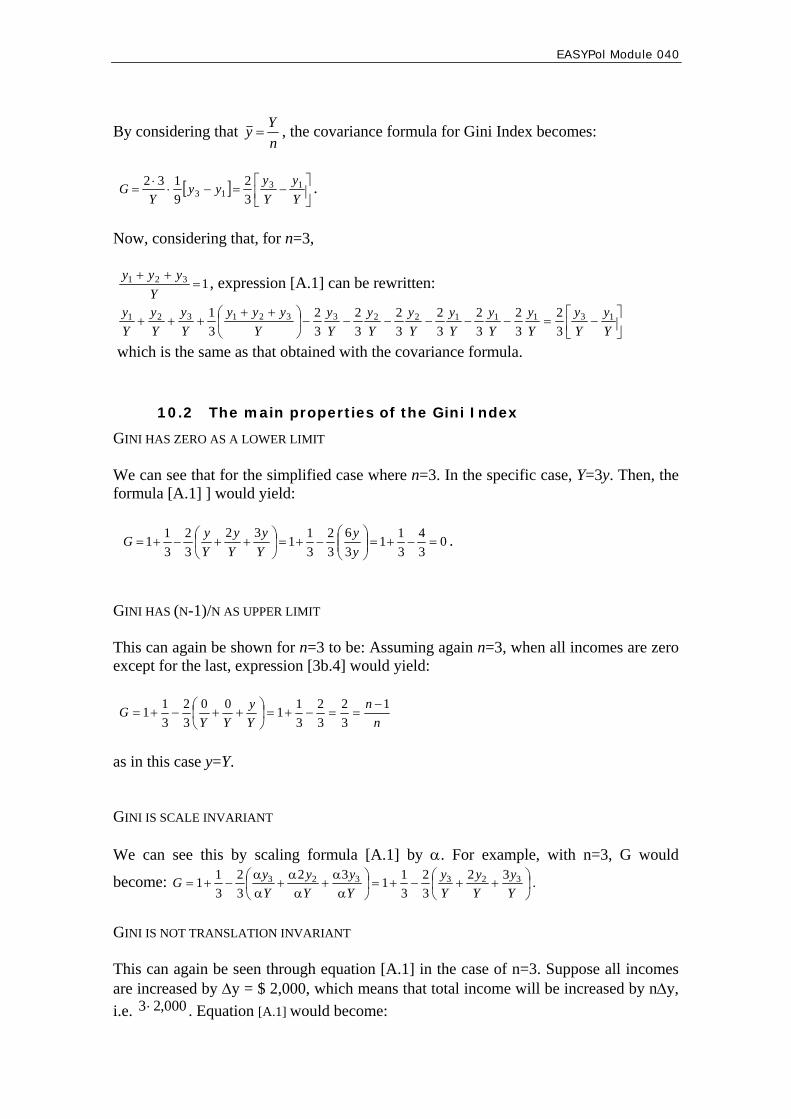
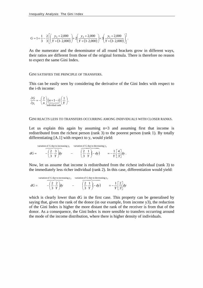
EASYPol Module 040 Analytical Tools
24
11 REFERENCES AND FURTHER READING
Anand S 1983 Inequality and Poverty in Malaysia Oxford University Press London
UK Cowell F 1977 Measuring Inequality Phillip Allan Oxford UK Dalton H 1920 The Measurement of Inequality of Incomes Economic Journal 30 Gini C 1912 Variabilitagrave e mutabilitagrave Bologna Italy Pigou AC 1912 Wealth and Welfare MacMillan London UK Sen AK 1973 On economic Inequality Calarendon Press Oxford UK Theil H 1967 Economics and Information Theory North-Holland Amsterdam The
Netherlands Yitzhaki S 1983 On the Extension of the Gini Index International Economic Review
24 617-628
Inequality Analysis The Gini Index 25
Module metadata
1 EASYPol module 040
2 Title in original language
English Inequality Analysis
French
Spanish
Other language
3 Subtitle in original language
English The Gini Index
French
Spanish
Other language
4 Summary
This tool addresses the most popular inequality index the Gini Index It discusses its characteristics and the link with another popular graphical tool of representing inequality the Lorenz Curve Extended version of the Gini Index with different weighting schemes are also discussed The use of the Gini Index and of its generalised versions is explained through a step-by-step procedure and numerical examples
5 Date
December 2006
6 Author(s)
Lorenzo Giovanni Bellugrave Agricultural Policy Support Service Policy Assistance Division FAO Rome Italy
Paolo Liberati University of Urbino Carlo Bo Institute of Economics Urbino Italy
7 Module type Thematic overview Conceptual and technical materials
Analytical tools Applied materials Complementary resources
8 Topic covered by Agriculture in the macroeconomic context the module Agricultural and sub-sectoral policies Agro-industry and food chain policies
Environment and sustainability Institutional and organizational development Investment planning and policies Poverty and food security Regional integration and international trade Rural Development
9 Subtopics covered by the module
10 Training path Analysis and monitoring of socio-economic impacts of policies
EASYPol Module 040 Analytical Tools
26
11 Keywords capacity building agriculture agricultural policies agricultural development development policies policy analysis policy impact anlaysis poverty food security analytical tool inequality inequality analysis inequality index inequality measures cost-benefit analysis gini index generalised gini index lorenz curve social welfare analysis