INDUSTRIAL STEEL PIPE SYSTEMS UNDER SEISMIC LOADING: A

COMPDYN 2011 3rd ECCOMAS Thematic Conference on

Computational Methods in Structural Dynamics and Earthquake Engineering M. Papadrakakis, M. Fragiadakis, V. Plevris (eds.)

Corfu, Greece, 25–28 May 2011

INDUSTRIAL STEEL PIPE SYSTEMS UNDER SEISMIC LOADING: A COMPARISON OF EUROPEAN AND AMERICAN DESIGN CODES

Gert J. Dijkstra1, Benjamin Francis1, Hildo van der Heden1 and Arnold M. Gresnigt2

1Tebodin Netherlands BV P.O. Box 16029 • 2500 BA The Hague • The Netherlands

[email protected] • [email protected] • [email protected]

2Delft University of Technology P.O. Box 1548 • 2600 GA Delft • The Netherlands

[email protected]

Keywords: Piping System, Seismic Design, Case Studies, American Standards, European Standards, Static and Dynamic Calculation, Pipeline.

Abstract. In the framework of the INDUSE project, which aims at innovative design method-ologies for the seismic design of industrial equipment and piping systems, case studies have been carried out, performing static and dynamic seismic analyses for two existing steel pipe-line systems including steel supporting structures, situated in an area of moderate seismic ac-tivity: a) A long aboveground 10" ammonia transmission line situated on sleepers with a vertical

expansion loop and ending with a fixed point. The system may be typical for long distance above ground pipelines and for pipelines on jetties.

b) A 20" gas transmission pipeline at the interface of a buried pipeline section and an above ground piping section, including a branch connection, a vertical spring support structure and a fixed point, e.g. a tank nozzle. This system is typical for many plant piping systems.

The calculations were made using commercially available software. Both simplified static equivalent (‘uniform load method’) calculations as well as dynamic calculations were made in accordance with American (ASCE-7) and European (EN1998 and EN13480) earthquake design standards to identify differences in approach, differences in resulting seismic response spectra and differences in calculated results. The dynamic and static calculations were made with Caesar II software.

The results of the calculations are presented. Conclusions and recommendations are given with respect to: - The differences between existing earthquake design codes. - The validity of the use of the "static equivalent (uniform load) method". - The need to include guidelines for design and modeling in the next revisions of existing

seismic design standards for (above ground) industrial piping systems.

Gert J. Dijkstra, Benjamin Francis, Hildo van der Heden and Arnold M. Gresnigt

2

1 INTRODUCTION

In the framework of the INDUSE project [1], which aims at innovative design methodolo-gies for the seismic design of industrial equipment and piping systems, a case study was car-ried out, performing static and dynamic seismic analyses for two existing steel pipeline systems including steel supporting structures, situated in an area of moderate seismic activity:

a) A long aboveground 10" ammonia transmission line situated on sleepers with a verti-cal expansion loop and ending with a fixed point. The system may be typical for long distance above ground pipelines and for pipelines on jetties.

b) A 20" gas transmission pipeline at the interface of a buried pipeline section and an above ground piping section, including a branch connection, a vertical spring support struc-ture and a fixed point, e.g. a tank nozzle. This system is typical for many plant piping systems.

Both simplified static equivalent (‘uniform load method’) calculations as well as dynamic calculations were made in accordance with American (ASCE-7 [2]) and European (EN1998-1/4 [3],[4] and EN13480 [5]) earthquake design standards to identify differences in approach, differences in resulting seismic response spectra and differences in calculated results. The dy-namic and static calculations were made with commercially available (Caesar II) software.

2 INVESTIGATED PIPE SYSTEMS

2.1 Ammonia transmission line

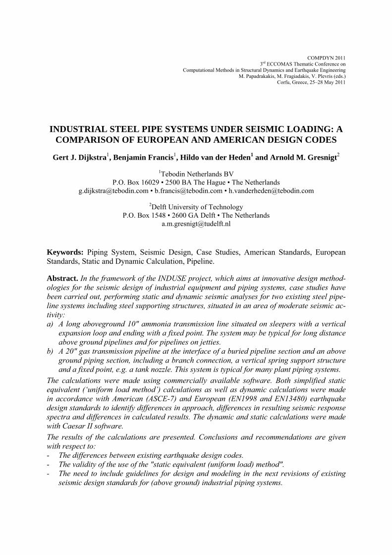
The 10" pipeline to transport liquid ammonia is located in the Algerian desert. It is roughly 9 km long. For practical reasons the modeled section (Figure 1) is 400 m long. Node 1 is modeled as a fixed point, node 650 allows only for rotation. As is expected with such long pipelines, there are loops to deal with thermal- and pressure expansion. Two vertical expan-sion loops have been modeled. The spacing between the supports in the straight pipe sections is not uniform to avoid creating any standing waves when the pipe is vibrating at a mode of its natural frequency. Relevant pipe and process data are given in Table 1.

Figure 1: System layout and node numbers Liquid Ammonia line.


3

Pipe material Steel A333 Gr.6

Pipe Diameter / wall thickness 10" / Std Tensile strength, Rm 415 Nmm-2 Yield strength, Re (65°C) 232 Nmm-2 Design pressure 25 bar(g) Design temperature 65/-35 °C Installation temperature 40 °C Corrosion Allowance 3 mm Medium/ density Liquid Ammonia, 880 kg/m3

Thermal Insulation 100 mm, PU Foam, 80 kg/m3

Table 1: Pipe and process data Ammonia line.

2.2 Gas transmission line

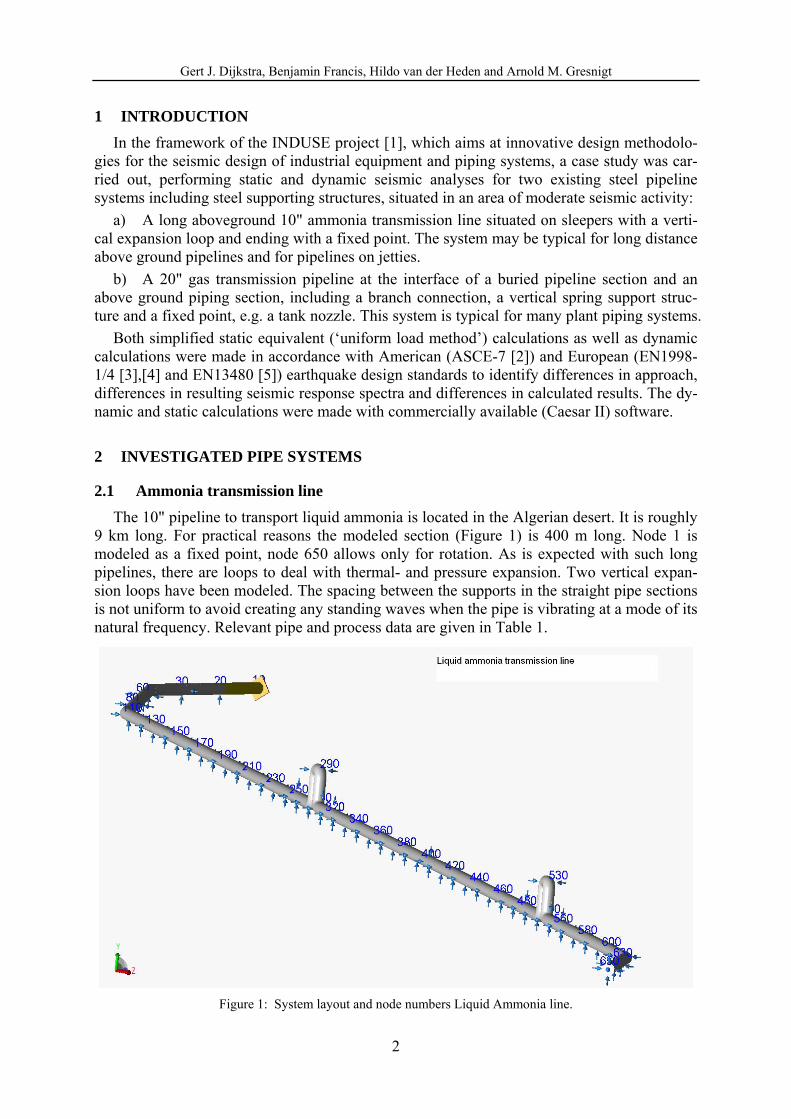
The gas transmission line includes an underground section and is modeled from a point underground to a (nozzle) connection (node 160) and a free end valve (node10) above ground (Figure 2). Relevant pipe and process data are given in Table 2.

Figure 2: System layout and node numbers Gas transmission line.

Pipe material 20" ; branch 16" Pipe Diameter / wall thickness Sch. 60 (16.6 & 20.6mm) Tensile strength, Rm 413 Nmm-2 Yield strength, Re (65°C) 241 Nmm-2

Design pressure 73.5 bar(g) Design temperature 80 °C Installation temperature 40 °C Corrosion Allowance 1.6 mm Medium/ density Natural gas, 1 kg/m3

Table 2: Pipe and process data Gas transmission line.

The pipe is supported by two steel structures, which add a finite amount of stiffness, which have been modeled in Caesar II. The static calculation was made according to ASME B31.8:2007 [8]. For the buried pipe section, the underground pipe modeler in Caesar II calcu-


4

lates pseudo-supports along the pipe to mimic the behavior of the soil acting on the buried pipe. The buried pipe support distance is pre-calculated by Caesar II, based on pipe stiffness and soil characteristics. Where it is not supported, the buried pipe had six degrees of freedom. However, these are considered negligible due to the pseudo-supports.

3 MODELING THE PIPE SYSTEM BEHAVIOUR UNDER SEISMIC LOAD BY SIMPLIFIED STATIC EQUIVALENT (UNIFORM LOAD) ANALYSIS

3.1 General

Commonly used international standards for seismic design allow for a simplified static equivalent analysis method to deduce a loading value to apply to the pipe system in order to model the seismic behavior. Using this method, the systems own response to different vibrat-ing frequencies and damping rates is ignored and instead the displacements and forces in the piping system are calculated using a single equivalent static accelerating force for each prin-cipal direction (X, Y and Z) of the seismic movements. The magnitude of the static loading is directly proportional to the element weight. Earthquake load magnitudes are given in terms of the gravitational acceleration constant, g, i.e. if an earthquake is modeled as having a 0.2 g load in a particular direction, then a factor of 0.2 of the systems weight is turned into a uni-form load and applied in that particular direction. Within the framework of this study this method was worked out for the relevant American and European codes.

3.2 Uniform load analysis according to American standard ASCE-7

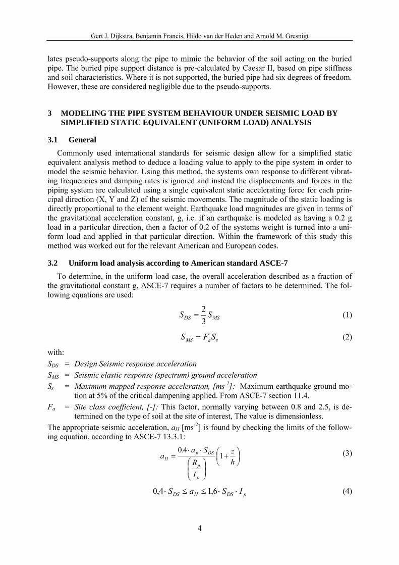
To determine, in the uniform load case, the overall acceleration described as a fraction of the gravitational constant g, ASCE-7 requires a number of factors to be determined. The fol-lowing equations are used:

MSDS SS3

2 (1)

saMS SFS (2)

with:

SDS = Design Seismic response acceleration

SMS = Seismic elastic response (spectrum) ground acceleration

Ss = Maximum mapped response acceleration, [ms-2]: Maximum earthquake ground mo-tion at 5% of the critical dampening applied. From ASCE-7 section 11.4.

Fa = Site class coefficient, [-]: This factor, normally varying between 0.8 and 2.5, is de-termined on the type of soil at the site of interest, The value is dimensionless.

The appropriate seismic acceleration, aH [ms-2] is found by checking the limits of the follow-ing equation, according to ASCE-7 13.3.1:

h

z

I

R

Sa.a

p

p

DSpH 1

40 (3)

pDSHDS ISaS 6,14,0 (4)


5

with:

Ip = Importance factor - : This value ranges from 1-1.5 and relates to the occupancy category which itself is dictated by the amount of risk present based on ASCE-7 table 1-1.

z/h = Component elevation ratio - : The ratio of height of the structure at the point of at-tachment over the average height of the supporting structure.

ap = Component amplification factor - : Constant, based on the relationship between the piping response and the structural response for a piping system, which can be related to the response of a system as affected by the type of seismic attachment. It is deter-mined from table 13.6-1 from ASCE-7. It is an arbitrary constant that varies depend-ing on the mechanical components in question.

Rp = Component response modification factor, -: Similar to ap this is an arbitrary con-stant that varies depending on the mechanical components in question. This value, too, is taken from ASCE-7 table 13.6-1.

Once aH has been determined, the horizontal force Fp is deduced by introducing the total weight of the system, Wp, to the horizontal acceleration term in the equation:

pHp WaF (5)

The uniform load shall be applied to the static analysis, independently in at least two or-thogonal horizontal directions in combination with the service loads associated with the com-ponent. An additional vertical component, which is 0.2 of the horizontal loading, is applied in combination with the two separate horizontal cases.

3.3 Uniform load analysis according to the European code EN13480

EN1998-1 and -4 do not specify an equivalent static uniform load method as an alternative to dynamic analysis, however the European piping design code EN13480 calculates the uni-form load magnitude in a similar way like ASCE-7. The acceleration component of the equa-tion is based on the maximum value arising from the earthquake. The static equivalent acceleration, acqi can be found by the following equation from EN13480-3:2002, A.2.1.2:

1aka icqi (6)

with:

ai is the acceleration defined for the level in direction i, and ki is a factor, dependent on the degree of analyses of the natural frequencies of the system Importance factor -.

ki = 1 when system’s natural frequencies of the piping system can be shown not to coincide within 10% of the peak vibration frequencies in the response spectrum of the struc-ture (or the peak ground acceleration if the pipe work is not mounted on a structure or building.

ki = 1.5 where no check on the coincidence of piping and structure vibration characteristics has been undertaken.

For this study the factor k i= 1.5 is used.

3.4 Resulting design acceleration (Uniform load method, Ammonia and Gas pipeline)

To match the original design calculations according the Algerian Earthquake resistance code RPA99:2003, made with the respective software packages AutoPIPE and ROHR2 for the Ammonia transfer line the gas transmission line, a uniform load of 0.2g and 0.14g hori-


6

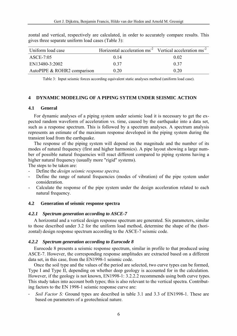
zontal and vertical, respectively are calculated, in order to accurately compare results. This gives three separate uniform load cases (Table 3):

Uniform load case Horizontal acceleration ms-2 Vertical acceleration ms-2

ASCE-7:05 0.14 0.02

EN13480-3:2002 0.37 0.37

AutoPIPE & ROHR2 comparison 0.20 0.20

Table 3: Input seismic forces according equivalent static analyses method (uniform load case).

4 DYNAMIC MODELING OF A PIPING SYTEM UNDER SEISMIC ACTION

4.1 General

For dynamic analyses of a piping system under seismic load it is necessary to get the ex-pected random waveform of acceleration vs. time, caused by the earthquake into a data set, such as a response spectrum. This is followed by a spectrum analyses. A spectrum analysis represents an estimate of the maximum response developed in the piping system during the transient load from the earthquake.

The response of the piping system will depend on the magnitude and the number of its modes of natural frequency (first and higher harmonics). A pipe layout showing a large num-ber of possible natural frequencies will react different compared to piping systems having a higher natural frequency (usually more "rigid" systems). The steps to be taken are: - Define the design seismic response spectra. - Define the range of natural frequencies (modes of vibration) of the pipe system under

consideration. - Calculate the response of the pipe system under the design acceleration related to each

natural frequency.

4.2 Generation of seismic response spectra

4.2.1 Spectrum generation according to ASCE-7

A horizontal and a vertical design response spectrum are generated. Six parameters, similar to those described under 3.2 for the uniform load method, determine the shape of the (hori-zontal) design response spectrum according to the ASCE-7 seismic code.

4.2.2 Spectrum generation according to Eurocode 8

Eurocode 8 presents a seismic response spectrum, similar in profile to that produced using ASCE-7. However, the corresponding response amplitudes are extracted based on a different data set, in this case, from the EN1998-1 seismic code.

Once the soil type and the values of the period are selected, two curve types can be formed, Type I and Type II, depending on whether deep geology is accounted for in the calculation. However, if the geology is not known, EN1998-1: 3.2.2.2 recommends using both curve types. This study takes into account both types; this is also relevant to the vertical spectra. Contribut-ing factors to the EN 1998-1 seismic response curve are:

- Soil Factor S: Ground types are described in table 3.1 and 3.3 of EN1998-1. These are based on parameters of a geotechnical nature.


7

- Damping Factor η: This is the damping correction factor of which the source is internal friction of the materials, imperfect connections between components, sliding friction, and other features. This is governed by the following expression:

0.555

10

(7)

where ξ is the damping ratio of the structure [%]. Throughout this study, the damping ratio was set at 5%, according to EN13480-1 A.2.1.6 where a value of 5% is used for systems with a frequency below 10Hz, thus rendering the damping factor to be unity throughout.

- Behavior Factor q: This is the ratio between the peak ground acceleration (PGA) that produces the ultimate displacement or rotation and the PGA that produces the yielding of the first point of the structure under consideration.

- Ground Acceleration ag: The design ground acceleration on type A ground is defined as:

gRg aa 1 (8)

Where γ1 is the topographic amplification factor, which is always greater than 1.

4.2.3 Vertical design spectrum A major difference between the ASCE-7 and EN1998-1 codes is the magnitude of a vertical com-

ponent to the calculation. According ASCE-7 the vertical spectrum is set to 20% of the amplitude of the horizontal design response spectrum across the entire period range.

According to EN1998-1 two types of curves can be applied, as seen in the design spectrum for the horizontal component, namely type I & II. However, a behavior factor appears in the equation and two ground acceleration values are mentioned in the code in table 3.4 of EN1998-1, resulting in the verti-cal spectra, given in fig. 3a and 3b.

4.2.4 Soil type selection The soil types selected as a basis for the calculations according ASCE 7 and EN1998-1 were best

matched to each other, leading to the choice for soil type C (ASCE-7) and soil type B (EN1998-1) re-spectively.

Soil type C from ASCE-7 is described as "very dense soil and soft rock" with a wave velocity range, as listed in table 20.3-1 ASCE-7, lying between 365-762 ms-1. EN1998-1, which is a little bit more descriptive, describes soil type B as "Deposits of very dense sand, gravel or very stiff clay, at least several tens of meters in thickness, characterized by a gradual increase of mechanical properties with depth." The shear wave velocity range in table 3.1 of EN1998-1 for soil type B is 360-800 ms-1.

For both codes shear wave velocity associated with each soil type is determined in the same way, the difference being constants used to describe the same values. The following equation represents the way that shear wave velocity, vs,30 – at 30 meters - is presented in table 3.1 (2) of EN1998-1. ASCE-7-05 presents in equation 20.4-1 an identical manner, with the thickness term hi presented as di.

,Ni i

is,

v

hv

1

30

30 (9)

4.2.5 Input parameters and design seismic spectrum generation

On basis of the foregoing, the input parameters for generating the design seismic response spectra are generated, Table 4 and Table 5). This results in horizontal and vertical design seis-mic response spectra according to both the ASCE code and the EN1998-1 code. Figure 3 and Figure 4 show the calculated horizontal and vertical design response spectra.


8

CURVE TYPE / VALUE

Parameter EN1998-1 Type I (Horizontal)

Type I (vertical)

Type II (Horizontal)

Type II (Vertical)

Reference EN1998-1

Soil Type B B B B Table 3.1

Importance factor, γ1 1.2 1.2 1.2 1.2 Table 2.1(3)

Ground acceleration, aG 0.25 0.9 0.25 .45 n/a

Soil factor, S1) 1.2 n/a 1.35 n/a Table 3.2

TB1) (start of acc. plateau) 0.15 0.05 0.05 0.05 Table 3.2

TC1)

(end of acc. plateau) 0.5 0.15 0.25 0.15 Table 3.2

TD1) 2 1 1.20 1 Table 3.2

Behavior factor, q 3 3 3 3 Table 6.1 1) Dependent on soil type

Table 4: Input parameters Seismic design spectra EN1998-1.

Parameter ASCE-7 Value Reference ASCE-7

Soil Type C Table 20.3-1

Importance factor, Ip 1.25 Table 11.5-1

Site coefficient, FA 1.1 Table 11.4-1

Site coefficient, FV 1.5 Table 11.4-2 Maximum considered earthquake acceleration parameter, Ss

0.75 Table 11.4-1

Maximum considered earthquake acceleration parameter, S1

0.3 Table 11.4-2

Component amplification factor, ap 2.5 Table 13.6-1

Response modification factor, Rp 12 Table 13.6-1

Elevation ratio, z/h 1 n/a

Table 5: Input parameters Seismic design spectra ASCE-7.

For the liquid ammonia pipeline, Caesar II calculated 250 relevant modes of vibration and periods up to 0.866 seconds. Compared to this (cross country) pipeline, most plant piping sys-tems will be smaller and more rigid (more supporting) resulting in fewer relevant modes of vibration.

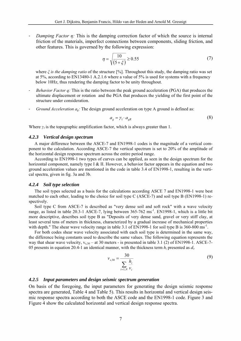
To be able to see how much influence each spectra has on the piping systems output, one must look at the spectra’s period in comparison to the system’s modes of natural frequency. As can be seen in fig 3a, the blue shaded region of the curve represents the range in which this particular system’s natural frequencies lie; the bold lines are sample modes which have been highlighted. The region outside of the shaded area is above a certain cut-off period, which translates for the ammonia line to 0.866 Seconds, which is 1.154 Hz – the 1st mode of the systems natural frequency. Although the peak of the type II horizontal curve is higher, the maximum acceleration with which Caesar II calculates the system at the 1st mode of vibration


9

is 0.15 ms-2 for the type I horizontal curve. The pipes natural frequency is the determining factor on how much the spectra influence the results.

The higher the mode of vibration the lower the periodicity, thus there will be a particular mode of vibration which matches the peaks of each curve. The vertical lines on the graph be-low represent the modes of vibration mode 1 can be seen at 0.866 seconds, the 2nd mode is visible at 0.459 seconds, the 25th and 100th modes are also represented on the graph at 0.132 and 0.060 seconds respectively. Similarly the same can be shown when comparing the ASCE-7 curve with the EN1998-1 curves.

Figure 3: Horizontal and vertical seismic design spectra according EN1998-1 and ASCE-7, with natural fre-

quency range (blue shaded) of the ammonia pipeline system.

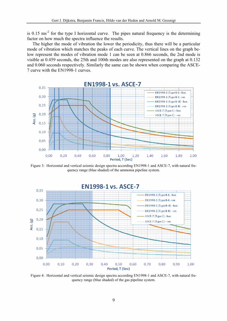
Figure 4: Horizontal and vertical seismic design spectra according EN1998-1 and ASCE-7, with natural fre-

quency range (blue shaded) of the gas pipeline system.


10

The number of modes of the natural frequencies present in the gas transmission line, calcu-lated according 4.3, are much fewer compared to the liquid ammonia transmission line. This is expected as the system is more rigid and shorter. Similarly to the curves seen in dynamic analysis of the liquid ammonia pipeline, Figure 4 shows the relevant area of the curve for the natural gas system.

It’s quite clear to see from Figure 3 that natural frequency mode 1 (T~0.3 S) of the pipe system corresponds to the plateau of the response spectra EN1998, type I and ASCE 7, pro-ducing higher acceleration forces (and stress results) compared to EN1998-1 (type 2) spectra, though the latter has a larger plateau compared to EN1998 (type 1).

4.3 Modeling and determination of the range of natural frequencies of the pipe system

Calculation of natural frequencies

The system’s modes of vibration will respond to the load in the exact same nature as a sin-gle degree of freedom oscillator with the generation of the response spectra, as it obeys New-ton’s second law for damped harmonic oscillators.

xkdt

dxc

dt

xdmF(t)

2

2

(10)

When calculating the modes of vibration and the fundamental frequency of the system, Caesar II, being the software package used for the dynamic calculations, will set the driving force to be zero. Also the damping factor is zero which eliminates the second term of the equation and allows Caesar II to solve the equation harmonically. For simple harmonic mo-tion the displacement can be described as:

tSin ωωxdt

xd

tCos ωωxdt

dx

tSin ωxx

202

2

0

0

(11)

Therefore, substituting in the displacement to the acceleration equation along with the stiffness and mass gives the following equation which Caesar II can use to determine the fun-damental frequency:

xωdt

xd 2

2

2

m

kω (12)

The system’s overall response can be described in terms of displacement, which is shown in the equation below:

2ω

a

ω

vx

(13)

Where x is the displacement from response spectrum at frequency f, v is the velocity, ω is the angular frequency at which response spectrum parameters are taken and a is the accelera-tion from response spectrum at frequency. Caesar II completes the following steps:

1. An Eigen solver algorithm is used to extract the exact modes of vibration from the sys-tem. The subsequent modes have a characteristic frequency and mode shape.


11

2. The maximum response of each mode under the applied load is determined from the spectrum value corresponding to the mode’s natural frequency.

3. The total system response is determined by summing the individual modal responses us-ing the square root of the sums of the squares method, where Ri is the total response in direction, i, Rmi is the peak response due to mode m and n is the total number of signifi-cant modes for the particular system.

2

1mi

n

mi RR

(14)

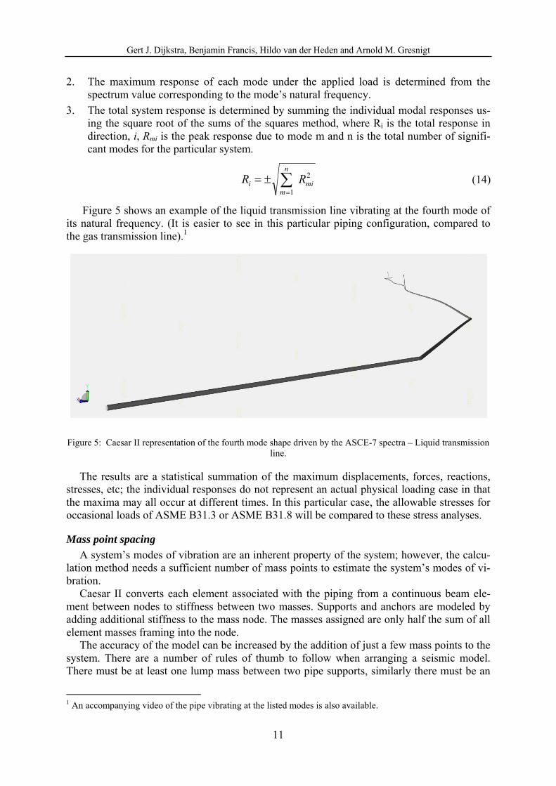
Figure 5 shows an example of the liquid transmission line vibrating at the fourth mode of its natural frequency. (It is easier to see in this particular piping configuration, compared to the gas transmission line).1

Figure 5: Caesar II representation of the fourth mode shape driven by the ASCE-7 spectra – Liquid transmission line.

The results are a statistical summation of the maximum displacements, forces, reactions, stresses, etc; the individual responses do not represent an actual physical loading case in that the maxima may all occur at different times. In this particular case, the allowable stresses for occasional loads of ASME B31.3 or ASME B31.8 will be compared to these stress analyses.

Mass point spacing

A system’s modes of vibration are an inherent property of the system; however, the calcu-lation method needs a sufficient number of mass points to estimate the system’s modes of vi-bration.

Caesar II converts each element associated with the piping from a continuous beam ele-ment between nodes to stiffness between two masses. Supports and anchors are modeled by adding additional stiffness to the mass node. The masses assigned are only half the sum of all element masses framing into the node.

The accuracy of the model can be increased by the addition of just a few mass points to the system. There are a number of rules of thumb to follow when arranging a seismic model. There must be at least one lump mass between two pipe supports, similarly there must be an

1 An accompanying video of the pipe vibrating at the listed modes is also available.


12

even mass distribution on bends and where there is concentration of mass, such as a flange, valve or tee. Table 6 gives the ratio to the exact solution of the number of significant nodes Caesar II can calculate depending on the number of nodes between supports.

Nodes (including end nodes) Ratio (%)

2 69.6 3 88.5 4 93.7

5 95.7 10 97.9

Table 6: Influence of mass point spacing on calculation accuracy.

In the calculation of the liquid ammonia transfer line, having a high number of possible vi-bration modes, extra nodes had to be added between the supports. The average mass spacing needed is approximately 5 nodes between each supports, which gives approximately 95% ra-tio to the exact solution of the modes of the natural frequency. The approximate distance at which to split the sections of pipes is given by the following equation:

4

13

2.9

W

tDL (15)

where: L = distance between two consecutive lumped masses (mm). D = outside diameter of pipe (mm). T = wall thickness of the pipe (mm). W = weight per unit length of the pipe (kg.m-1).

The results are only a guide, as in some cases it is impossible to split the nodes into the re-quired distance because of the piping geometry. The lumped mass distance for the liquid am-monia transmission line was calculated to be 387 mm and the distance for the natural gas transmission line was calculated to be 480 mm.

Support modeling

Throughout both models, the types of supports which have been modeled are simplistic slide or guide supports. Only the frictional effect has been modeled along with the physical barrier which prevents the pipe moving in the specified direction. This technique is common place in pipe modeling. Where a support is very long, occasionally the stiffness factor will be modeled, however, this does not occur in the two systems studied. The aforementioned sys-tem where a steel structure has been modeled Caesar II takes into consideration the stiffness associated with the frame. When modeling the supports as slide or guide supports, the stiff-ness factor was assumed to be negligible.

Restrictions to modeling

Caesar II does not model any ‘slapping’ – where the pipe lifts up from a support in one time frame and slaps down on the support. The pipe must be restricted or free to move. The restraints which are non-linear in the static cases must be made active or inactive to enable an


13

accurate dynamic analysis. It is possible to set non-linear restraints to a configuration found in the static results.

Another effect which is non-linear is the force produced from friction. These must also be set to be linear. A default setting for II is to model the supporting as having no frictional ef-fects. If desired, Caesar II can approximate the frictional force in the dynamic case by assum-ing a +Y restraint the frictional value would instead be added to the X and Z directions and a spring support would be included.

It should be noted that the slapping effect does not arise in a situation where a spring hanger has been modeled in the static stage of the calculation. Therefore, if in one of the load cases a lifting of the pipe occurs at the spring support it will still be modeled as a support at the dynamic stage of the calculation.

5 CALCULATION RESULTS AND DISCUSSION FOR THE AMMONIA TRANSMISSION LINE

The effect of design acceleration on pipe stresses, forces and bending moments was calcu-lated with special focus on the end nozzles.

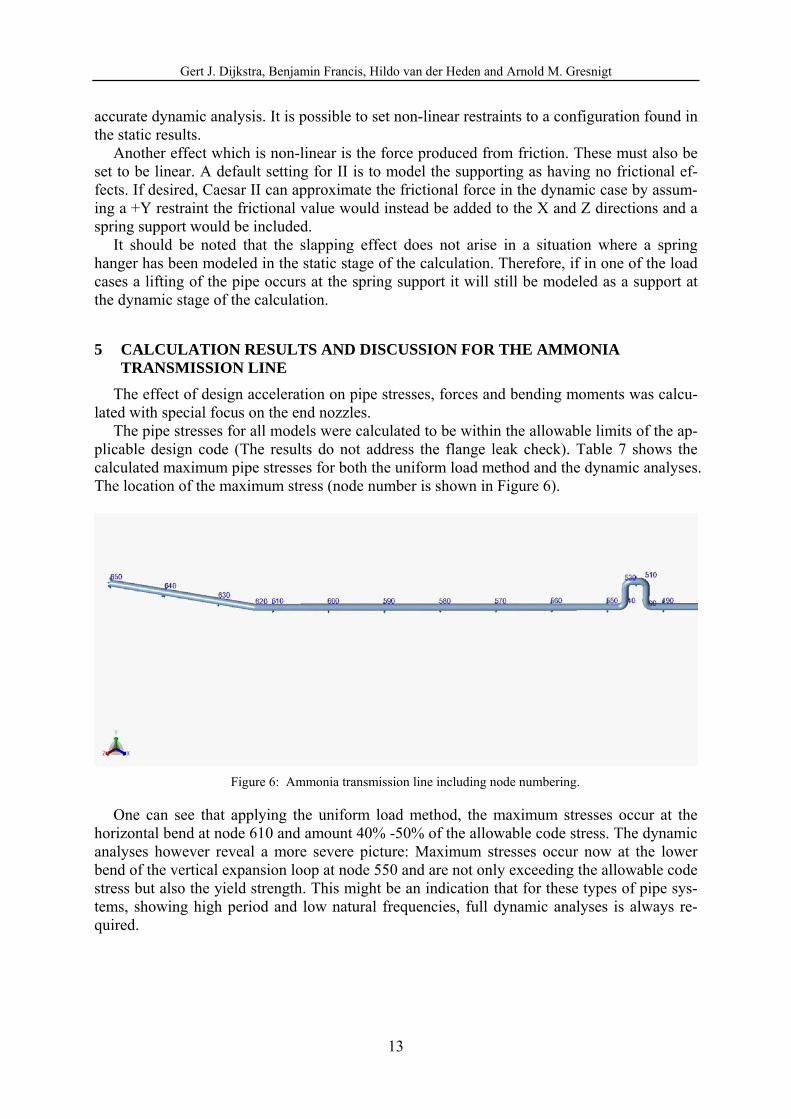
The pipe stresses for all models were calculated to be within the allowable limits of the ap-plicable design code (The results do not address the flange leak check). Table 7 shows the calculated maximum pipe stresses for both the uniform load method and the dynamic analyses. The location of the maximum stress (node number is shown in Figure 6).

Figure 6: Ammonia transmission line including node numbering.

One can see that applying the uniform load method, the maximum stresses occur at the horizontal bend at node 610 and amount 40% -50% of the allowable code stress. The dynamic analyses however reveal a more severe picture: Maximum stresses occur now at the lower bend of the vertical expansion loop at node 550 and are not only exceeding the allowable code stress but also the yield strength. This might be an indication that for these types of pipe sys-tems, showing high period and low natural frequencies, full dynamic analyses is always re-quired.


14

Load case / Design seismic spectrum

Type of calculation

Maximum stress in node

Stress [Nmm-2] (vibration mode) 2)

Allowable stress [Nmm-2] (ASME B31.3)

Ratio [%]

RPA99:2003 (AutoPIPE)

Uniform load

610 71.3 183.4 38.9

ASCE-7 Uniform load

610 66.1 183.4 36.0

Dynamic 550 239.4 (1) 183.4 130.5

EN13480 Uniform load

610 91.3 183.4 49.8

EN1998-1 (Type I)

Dynamic 550 275.1 (1) 183.4 150.0

EN1998-1 (Type II)

Dynamic 550 354.3 (4) 183.4 138.8

Table 7: Calculation results for Ammonia transmission line.

Ammonia transmission line: Nozzle focus

Table 8 and Table 9 present the results for the forces and moments, calculated for respectively the uniform load cases and the dynamic cases on the nozzle (fixed point, e.g. a tank nozzle) situated at node 10 (Figure 2). Code F(x) [N] F(y) [N] F(z) [N] M(x) [Nm] M(y) [Nm] M(z) [Nm]

RPA99:2003 (AutoPIPE)

15755 -5613 2190 239 6069 7209

ASCE-7 14200 -5038 -1652 173 4482 6487

EN13480 22525 -6484 -4028 335 11905 8240

Table 8: UNIFORM LOAD METHOD: Forces and moments on the nozzle at node 10.

Code

F(x) [N] (mode)

F(y) [N] (mode)

F(z) [N] (mode)

M(x) [Nm] (mode)

M(y) [Nm] (mode)

M(z) [Nm] (mode)

ASCE-7 6620 (1) 1434 (14) 2037 (4) 458 (36) 7198 (14) 2529 (1)

EN1998-1 (Type I)

7247 (1) 2261 (1) 1894 (14) 418 (36) 6561 (14) 3910 (1)

EN1998-1 (Type II)

9048 (1) 3381 (1) 2168 (14) 514 (1) 7380 (14) 5788 (1)

Table 9: DYNAMIC ANALYSES: Forces and moments on the nozzle at node 10.

It can be seen that – for this particular location, in general the uniform load cases generate higher forces and bending moments, compared to the results of the dynamic analyses, EN13480 giving the most conservative results.

2) An accompanying video of the pipe vibrating at the listed modes is also available.


15

The maximum values for the dynamic cases occur at different vibration modes. Also differences between results for the different seismic spectra can be observed. In general the calculated forces and moments are rather low.

6 CALCULATION RESULTS FOR THE GAS TRANSMISSION LINE

The effect of design acceleration on pipe stresses, forces and bending moments was calcu-lated with special focus on tees and nozzles and on the influence of a steel support structure, modeled into the dynamic calculations.

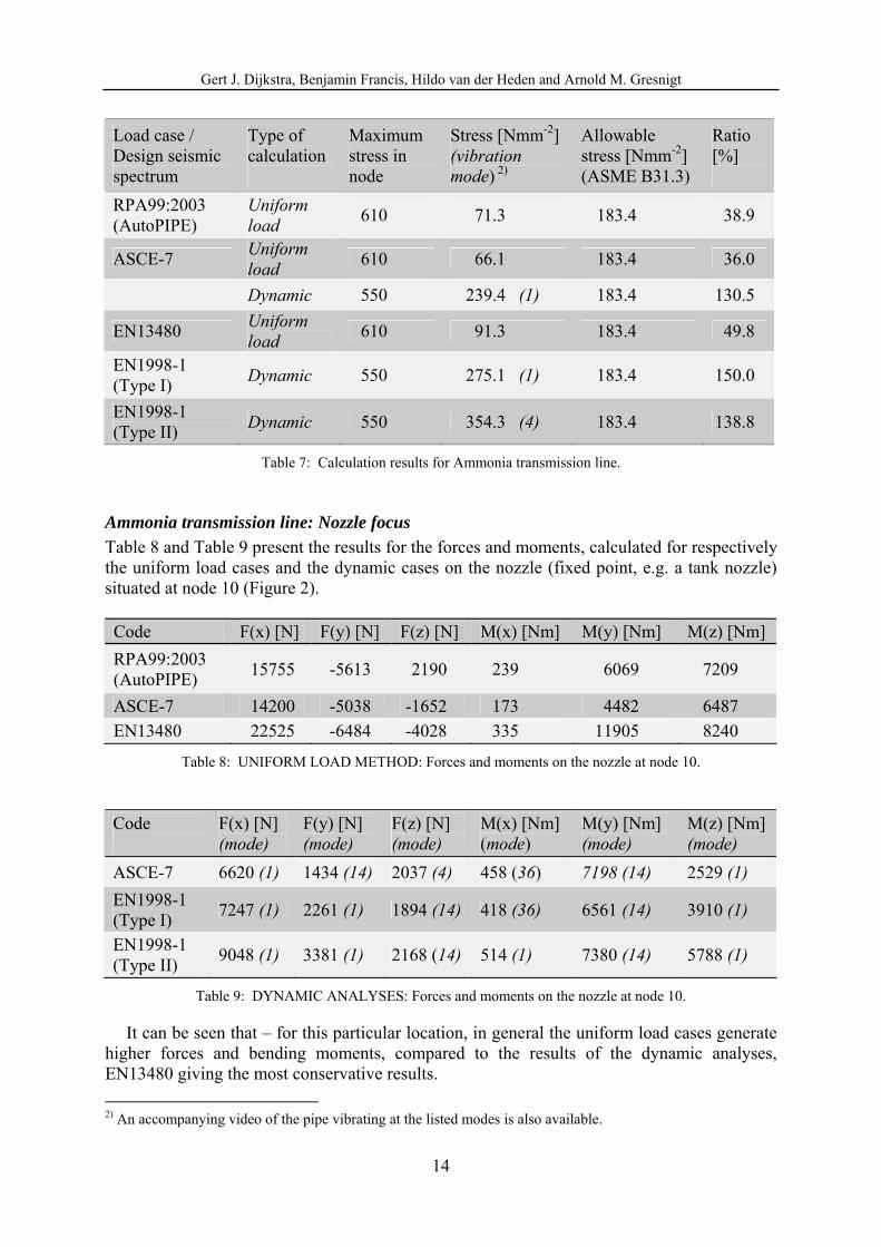
6.1 Calculations including modeling of the steel support structure

In this case the steel supporting structure was also modeled in Caesar II, allowing deforma-tions under load. Between the steel structure and the pipe a spring support is modeled. See Figure 7, (also for node numbers).

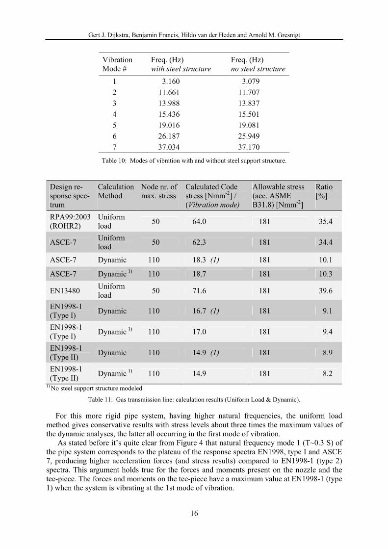
When removing the steel structure from the calculation, the system’s overall mass will be lower. This has an effect on the system’s natural frequency. Table 10 shows the calculated differences in the modes of vibration detected with and without the steel structure.

Table 11 presents the calculation pipe stresses for both the uniform load analysis and the dynamic analyses.

Figure 7: Detail of Gas transmission line, showing steel structure and node numbers.


16

Vibration Mode #

Freq. (Hz) with steel structure

Freq. (Hz) no steel structure

1 3.160 3.079

2 11.661 11.707

3 13.988 13.837

4 15.436 15.501

5 19.016 19.081

6 26.187 25.949

7 37.034 37.170

Table 10: Modes of vibration with and without steel support structure.

Design re-sponse spec-trum

Calculation Method

Node nr. of max. stress

Calculated Code stress [Nmm-2] / (Vibration mode)

Allowable stress

(acc. ASME B31.8) [Nmm-2]

Ratio [%]

RPA99:2003 (ROHR2)

Uniform load

50 64.0 181 35.4

ASCE-7 Uniform load

50 62.3 181 34.4

ASCE-7 Dynamic 110 18.3 (1) 181 10.1

ASCE-7 Dynamic 1) 110 18.7 181 10.3

EN13480 Uniform load

50 71.6 181 39.6

EN1998-1 (Type I)

Dynamic 110 16.7 (1) 181 9.1

EN1998-1 (Type I)

Dynamic 1) 110 17.0 181 9.4

EN1998-1 (Type II)

Dynamic 110 14.9 (1) 181 8.9

EN1998-1 (Type II)

Dynamic 1) 110 14.9 181 8.2

1) No steel support structure modeled

Table 11: Gas transmission line: calculation results (Uniform Load & Dynamic).

For this more rigid pipe system, having higher natural frequencies, the uniform load method gives conservative results with stress levels about three times the maximum values of the dynamic analyses, the latter all occurring in the first mode of vibration.

As stated before it’s quite clear from Figure 4 that natural frequency mode 1 (T~0.3 S) of the pipe system corresponds to the plateau of the response spectra EN1998, type I and ASCE 7, producing higher acceleration forces (and stress results) compared to EN1998-1 (type 2) spectra. This argument holds true for the forces and moments present on the nozzle and the tee-piece. The forces and moments on the tee-piece have a maximum value at EN1998-1 (type 1) when the system is vibrating at the 1st mode of vibration.


17

It is also noticed that, applying the uniform load method, the maximum stresses will occur at the T-Piece (node 50), whereas the dynamic analyses shows the maximum stresses occur in the upper bend at node 110.

Comparison of the calculated stresses with and without modeling of the steel support struc-ture shows that the differences are negligible. The (already very low) stresses in the pipe sys-tem are hardly influenced by the deformation of the steel structure under the horizontal (friction) load.

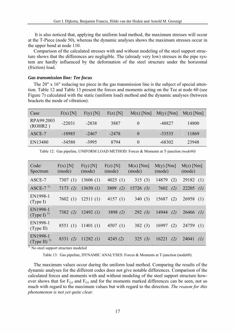
Gas transmission line: Tee focus

The 20" x 16" reducing tee piece in the gas transmission line is the subject of special atten-tion. Table 12 and Table 13 present the forces and moments acting on the Tee at node 60 (see Figure 7) calculated with the static (uniform load) method and the dynamic analyses (between brackets the mode of vibration).

Case F(x) [N] F(y) [N] F(z) [N] M(x) [Nm] M(y) [Nm] M(z) [Nm]

RPA99:2003 (ROHR2 )

-22031 -2838 3887 0 -48827 14800

ASCE-7 -18985 -2467 -2478 0 -33535 11869

EN13480 -34580 -3995 8794 0 -68302 23948

Table 12: Gas pipeline, UNIFORM LOAD METHOD: Forces & Moments at T-junction (node60)

Code/ Spectrum

F(x) [N] (mode)

F(y) [N] (mode)

F(z) [N] (mode)

M(x) [Nm] (mode)

M(y) [Nm] (mode)

M(z) [Nm] (mode)

ASCE-7 7307 (1) 13606 (1) 4025 (1) 315 (3) 14879 (2) 29182 (1)

ASCE-7 1) 7173 (2) 13650 (1) 3809 (2) 15726 (3) 7602 (2) 22205 (1)

EN1998-1 (Type I)

7602 (1) 12511 (1) 4157 (1) 340 (3) 15687 (2) 26958 (1)

EN1998-1 (Type I) 1) 7382 (2) 12492 (1) 3898 (2) 292 (3) 14944 (2) 26466 (1)

EN1998-1 (Type II)

8551 (1) 11401 (1) 4507 (1) 382 (3) 16997 (2) 24759 (1)

EN1998-1 (Type II) 1) 8331 (2) 11282 (1) 4245 (2) 325 (3) 16221 (2) 24041 (1)


Table 13: Gas pipeline, DYNAMIC ANALYSES: Forces & Moments at T-junction (node60).

The maximum values occur during the uniform load method. Comparing the results of the dynamic analyses for the different codes does not give notable differences. Comparison of the calculated forces and moments with and without modeling of the steel support structure how-ever shows that for F(y) and F(z) and for the moments marked differences can be seen, not so much with regard to the maximum values but with regard to the direction. The reason for this phenomenon is not yet quite clear.


18

Gas Transmission line: Nozzle focus

The nozzle situated at node 160 (see Figure 7), modeled as a fixed point, is a flange con-nection and therefore critical with regard to possible leakage. Table 14 and Table 15 represent the results of the forces and moments, calculated for the uniform load cases and for the dy-namic analyses (Between brackets the vibration mode).

Case F(x) [N] F(y) [N] F(z) [N] M(x) [Nm] M(y) [Nm] M(z) [Nm]

RPA99:2003 (ROHR2)

-2900 8066 -7013 -4736 8277 15637

ASCE-7 -2135 6229 -2477 -604 4519 14344

EN13480 -4908 9488 -2564 -127 5423 20083

Table 14: Nozzle focus, UNIFORM LOAD METHOD: Forces and Moments at the nozzle at node 160.

Spectrum

F(x) [N] (mode)

F(y) [N] (mode)

F(z) [N] (mode)

M(x) [Nm] (mode)

M(y) [Nm] (mode)

M(z) [Nm] (mode)

ASCE-7 4523 (1) 1668 (1) 16243 (1) 23074 (1) 20055 (1) 4999 (1)

ASCE-71) 4578 (1) 1419 (1) 16256 (1) 23183 (1) 20129 (1) 4967 (1)

EN1998-1 (Type I)

4307 (1) 1967 (1) 14949 (1) 21134 (1) 18414 (1) 5056 (1)

EN1998-1 (Type I) 1)

4331 (1) 1676 (1) 14881 (1) 21159 (1) 18397 (1) 5017 (1)

EN1998-1 (Type II)

4106 (1) 1802 (1) 13651 (1) 19167 (1) 16742 (1) 4568 (1)

EN1998-1 (Type II) 1)

4000 (1) 1406 (1) 13248 (1) 18738 (1) 16319 (1) 4358 (1)


Table 15: Nozzle focus, DYNAMIC ANALYSES: Forces and Moments at the nozzle at node 160.

The result for the nozzle forces are more or less in contradiction with the results of the cal-culated stresses in the pipes and with the forces and moments for the Tee. Here the maximum forces and moments occur in the dynamic cases. The maximum value for the moment being comparable with the result of the uniform load method (that is for the European code only), the maximum force calculated dynamically is clearly higher. The influence of the modeling of the steel substructure is negligible here.

7 CONCLUSIONS

Spectra comparison

The ASCE and EN seismic codes studied bear similar spectra, be it that that vertical spec-trum of ASCE 7-05 is considerably lower than the vertical spectra acc. to EN1998-1. The re-sults show that the EN1998-1 and ASCE-7 spectra in general yield similar stresses, forces and moments. This is due to the fact that the peaks occur roughly in the same periodicity as each other – relevant to a typical piping system with a natural frequency higher than 5Hz.


19

Dynamic vs. uniform load calculations

A direct comparison between the two methods of seismic calculations shows that in one case studied that the uniform load seismic calculations yielded more conservative results than the dynamic seismic calculations. This supports the already practiced method amongst engi-neers of rather calculating the uniform load stress then modeling the system dynamically. It is perhaps advantageous to carry out a uniform load seismic stress calculations with all earth-quake prone pipelines, provided the natural frequencies are high enough.

However, for loose and long pipe systems, a dynamic analysis is of fundamental impor-tance especially if the natural frequency is lower than 4-5Hz. In such cases the uniform load method might substantially underestimate the stresses and forces

Further investigations are required to determine safe borders for the application of the uni-form load method.

Influence of supporting structure

The effect seen when a steel supporting structure is included and modeled dynamically is that the system becomes more flexible, allowing the system to vibrate freely with the support-ing structure. In this particular case (the gas pipe system and the steel support structure being rather stiff), the influence on the natural frequencies appeared too little to make much differ-ence.

Influence of design

More important than the differences between codes in seismic design spectra is the design of the piping system This is the deciding factor in whether the system will be able to with-stand a particular seismic event. The philosophy of designing a system to be able to withstand loadings that occur during a static situation are that the right amount of flexibility should be included into the design e.g. to deal with expansion. This is often achieved by adding expan-sion loops, or by adjusting the geometry of the system. However, when a system is under seismic loading or any other dynamic situation which is likely to vibrate the system close to its natural frequency, it is desirable to design a system which is rigid. Provisions to prevent ‘slag’ between pipe and support may be necessary. This results in a trade-off between satisfy-ing the needs of the static and dynamic analysis requirements. Often an optimum design can be found by extensive stress analysis. It is recommended to include guidelines for design in the next revision of EN1998-4 and ASCE 7-05.

Influence of computer modeling

When performing dynamic analyses it is very important to apply the correct modeling practice in order to obtain reliable results, however this is not addressed in the present codes.

Non linear modeling of supports during dynamic analyses is not possible yet with com-mercially available software. For systems with more modes of vibration it is also very impor-tant that a sufficient number of nodes between the supports should be applied. It should be checked whether the computer model is able to deal with slag in the supports, etc. It is advised to include recommendations for modeling in the next revision of EN1998-4 and ASCE 7-05

ACKNOWLEDGMENT

This work was carried out with a financial grant from the Research Fund for Coal and Steel of the European Commission, within INDUSE project: "Structural Safety of Industrial Steel


20

Tanks, Pressure Vessels and Piping Systems Under Seismic Loading", Grant No. RFSR-CT-2009-00022.

REFERENCES

[1] INDUSE, Structural Safety of Industrial Steel Tanks, Pressure Vessels and Piping Sys-tems under Seismic Loading. RFCS research project, 2009-2012.

[2] ASCE 7-10, Minimum Design Loads for Buildings and Other Structures. American So-ciety of Civil Engineers, May 2010.

[3] EN1998-1, Eurocode 8: Design of structures for earthquake resistance - Part 1: General rules, seismic actions and rules for buildings, CEN, 2004.

[4] EN1998-4, Eurocode 8 – Design of structures for earthquake resistance – Part 4: Silos, tanks and pipelines, CEN, 2006.

[5] EN13480-3, Metallic industrial piping - Part 3: Design and calculation, CEN, 2002.

[6] ASME B31.3:2006, Code for Pressure Piping, Process Piping, ASME, New York.

[7] ASME B31.4:2006, Pipeline Transportation Systems for Liquid Hydrocarbons & Other Liquids, ASME, New York.

[8] ASME B31.8:2007, Gas Transmission & Distribution Piping Systems, ASME, New York.

[9] E.M. Marino, M. Nakashima, et al. Comparison of European and Japanese seismic de-sign of steel building structures, Engineering Structures 27 827-840, 2005.

[10] ROHR2, Pipe Stress Analysis Static and Dynamic Analysis (http://www.rohr2.com/)

[11] CAESAR II, Pipe Stress Analysis (http://www.codecad.com/Caesarii.htm)

[12] AutoPIPE, Piping Analysis (http://www.bentley.com/en-US/Products/Bentley+AutoPIPE/)

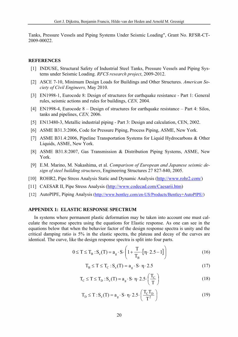
APPENDIX 1: ELASTIC RESPONSE SPECTRUM

In systems where permanent plastic deformation may be taken into account one must cal-culate the response spectra using the equations for Elastic response. As one can see in the equations below that when the behavior factor of the design response spectra is unity and the critical damping ratio is 5% in the elastic spectra, the plateau and decay of the curves are identical. The curve, like the design response spectra is split into four parts.

12.5η

T

T1Sa(T)S :TT0

BgeB (16)

2.5ηSa(T)S :TTT geCB (17)

T

T2.5ηSa(T)S :TTT C

geDC (18)

2

DCgeD T

TT2.5ηSa(T)S :TT (19)


21

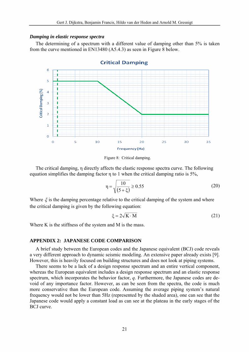
Damping in elastic response spectra

The determining of a spectrum with a different value of damping other than 5% is taken from the curve mentioned in EN13480 (A5.4.3) as seen in Figure 8 below.

Figure 8: Critical damping.

The critical damping, η directly affects the elastic response spectra curve. The following equation simplifies the damping factor η to 1 when the critical damping ratio is 5%,

0.55

ξ5

10η

(20)

Where is the damping percentage relative to the critical damping of the system and where the critical damping is given by the following equation:

MK2ξ (21)

Where K is the stiffness of the system and M is the mass.

APPENDIX 2: JAPANESE CODE COMPARISON

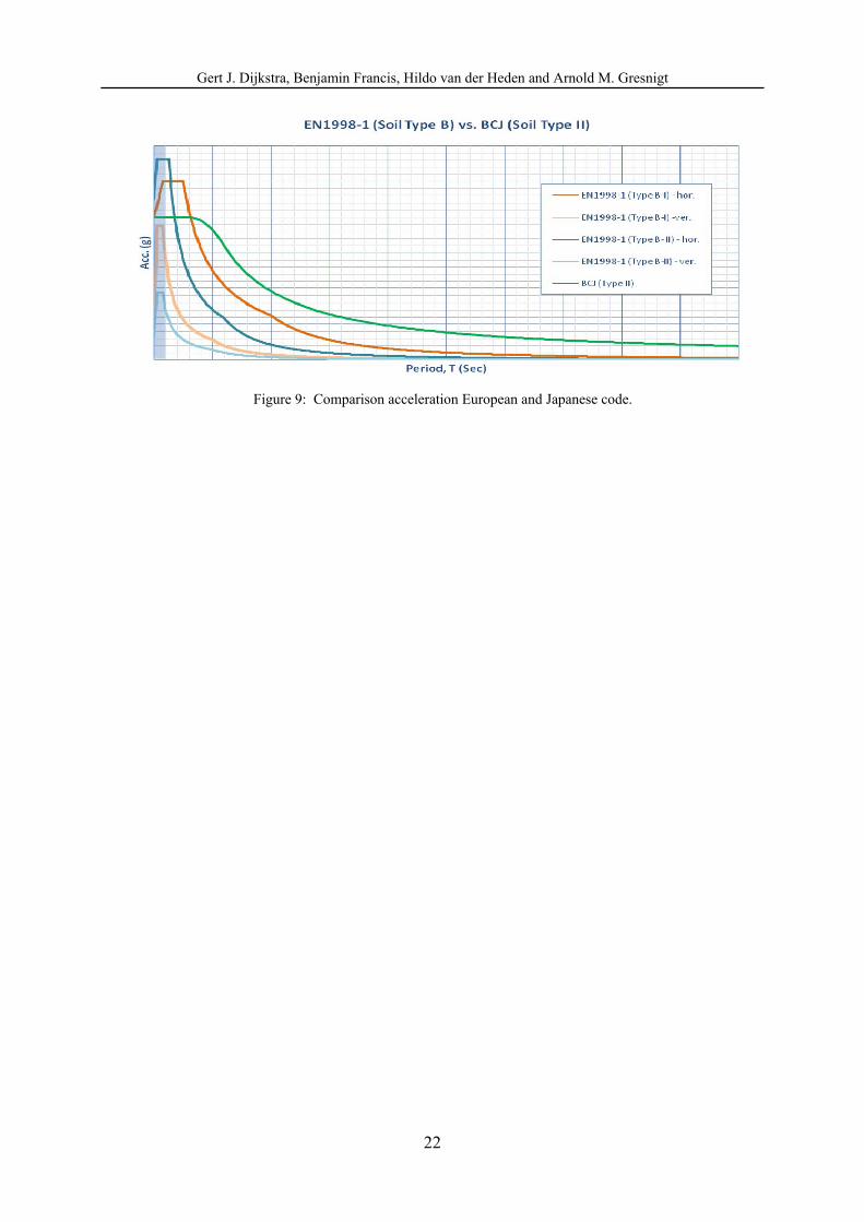
A brief study between the European codes and the Japanese equivalent (BCJ) code reveals a very different approach to dynamic seismic modeling. An extensive paper already exists [9]. However, this is heavily focused on building structures and does not look at piping systems.

There seems to be a lack of a design response spectrum and an entire vertical component, whereas the European equivalent includes a design response spectrum and an elastic response spectrum, which incorporates the behavior factor, q. Furthermore, the Japanese codes are de-void of any importance factor. However, as can be seen from the spectra, the code is much more conservative than the European code. Assuming the average piping system’s natural frequency would not be lower than 5Hz (represented by the shaded area), one can see that the Japanese code would apply a constant load as can see at the plateau in the early stages of the BCJ curve.


22

Figure 9: Comparison acceleration European and Japanese code.

INDUSTRIAL STEEL PIPE SYSTEMS UNDER SEISMIC LOADING: A

Documents

Transcript of INDUSTRIAL STEEL PIPE SYSTEMS UNDER SEISMIC LOADING: A