1

Industrial output fluctuations in developing countries: General equilibrium

consequences of agricultural productivity shocks

Hyojung Lee1

Purdue University

October 22, 2013

Abstract

This paper shows how agricultural productivity shocks can generate large industrial output fluctuations in poor

countries, using a static general-equilibrium model with Stone-Geary preferences. A negative shock to agricultural

productivity increases food prices, which affects manufacturing output through two channels: (1) meeting

subsistence requirements in the face of rising food prices causes poor households to shift consumption away from

manufactures; (2) capital and labor move away from manufacturing and into agriculture in response to the food price

increase. As a result, manufacturing output decreases in response to the decline in agricultural productivity. This

effect is larger the closer is income to the subsistence level. Calibration exercises show that the growth rate of

industrial output fluctuates significantly more in poor countries in response to changes in crop yields, a proxy for

agricultural productivity. In addition, I test the predictions empirically. I utilize annual manufacturing data and

instrument for crop yields using year-to-year changes in rainfall. The results show that a 1% decrease in crop yields

induced by shortages in rainfall decreases manufacturing output by 0.38%, capital investment by 1.56%, and

employment by 0.20% across 44 developing countries. Overall, crop yield variation (instrumented by rainfall

shocks) can explain about 28% of industrial output growth fluctuations in developing countries.

JEL codes: O12, O14, D58, E32

Keywords: two-sector general equilibrium models, economic fluctuations, volatility, instrumental variable

analysis, agricultural productivity

1 I am grateful to David Hummels for his continuous guidance and encouragement. I would like to thank Justin Tobias, Chong Xiang, Phillp Abbott, Mesbah Motamed, Ricardo Lopez, and Anson Soderbery for valuable comments and discussions. All

remaining errors are my own. Contact: Department of Economics, Purdue University, West Lafayette, IN 47907, USA. Tel: +1 (765)586-8592. E-mail: lee485@purdue.edu

2

1 Introduction

An important regularity in macroeconomic data is the frequent and large changes in developing

country growth rates, compared to the relatively stable growth rates in developed countries (Lucas, 1998).

Figure 1 highlights the negative relationship between aggregate output volatility, defined as the standard

deviation of output growth rates, and a country’s per capita income level. The negative association

between the two becomes stronger when manufacturing is considered separately, as shown in Table 1.

After controlling for population, regressing volatility on income reveals that a 10% decrease in per capita

GDP is associated with a 7% increase in industrial output volatility and only a 0.6% increase in aggregate

output volatility. This suggests that studying the causes of industrial output fluctuations can shed light on

aggregate volatility.

Higher output volatility can have negative effects on both the level and the growth path of

income.2 In poor countries, abrupt negative shocks to household incomes can be especially detrimental,

as income levels often barely exceed the level of subsistence.3 Furthermore, developing countries’ ability

to hedge against income fluctuations is limited by their underdeveloped financial system. For these

reasons, analyzing the causes of economic fluctuations in developing countries is particularly important.

A growing body of research has studied the high levels of output fluctuation in poor countries by

focusing primarily on supply side explanations. Many papers assume the existence of shocks that are

unknown or originate in the manufacturing sector and present plausible channels through which their

impact might be larger in poor countries. 4 For example, Koren and Tenreyro (2007) decompose industrial

output volatility and argue that developing countries specialize in more volatile sectors and experience

larger country-specific shocks. Koren and Tenreyro (2013) build a model in which firms in developed

countries use a greater number of input varieties, thus lowering their industrial output volatility through

diversification. Krishna and Levchenko (2012) and Kraay and Ventura (2007) argue that developed

countries exhibit lower volatility because they have a comparative advantage in more complex

technologies.5 In contrast, several papers in the finance literature argue the opposite, that highly

2 Van Wijnbergen (1984) points out that even a temporary decline in manufacturing can have a permanent negative impact on an

economy, assuming that growth occurs through a continuous accumulation of technological progress. In addition, Ramey and Ramey (1991) argue that volatility can reduce mean output ex-post if producers have to make decisions on resources before realizations of shocks. Similarly, Bernanke (1983) and Pindyck (1991) suggest that volatility can cause lower investments that take place in the form of sunk costs. 3 Effects of such shocks on households in poor countries include malnutrition, increased rate of infant mortality, disease, and long-term absence of child education. 4 While most papers focus on sector specific shocks, Tapia (2012) maintains that poor entrepreneurs have incentives to use financed resources for private consumption rather than investment in their firms, an outcome driven by information asymmetry.

He argues that this eventually leads to greater output volatility in poor countries. 5 Kraay and Ventura (2007) argue that industries that use advanced technologies are operated by skilled workers whose labor supply is inelastic, thus leading to less volatile business cycles in developed countries. In addition, Kose (2002) maintains that small open developing countries are largely affected by shocks to world prices as their production depends heavily on imported

3

productive projects are risky, subjecting firms in developed countries to greater shocks (e.g., Saint-Paul

1992; Obstfeld 1994).

This paper provides a novel explanation for industrial output fluctuations highlighting both

demand and supply side explanations. It focuses on a prominent characteristic of developing economies –

a large portion of income spent on food to satisfy subsistence needs – and shows how general equilibrium

linkages can generate larger industrial output fluctuations in response to shocks to agricultural

productivity. This paper departs from the literature in several ways. First, the previous literature does not

identify likely sources of shocks. Rather it only describes mechanisms through which some unidentified

shock is magnified for certain countries. In contrast, I focus on a specific and observable shock to

productivity. I use rainfall shocks to explain year-to-year changes in agricultural productivity in each

country, which allows me to measure the actual varying impact of the shock on manufacturing across

countries. Second, I propose a general equilibrium mechanism in which these shocks are transmitted to

industrial output. In the model, the effects are stronger for low-income countries, because non-homothetic

preferences magnify the consequences of falling agricultural yields in these countries. In contrast, the

literature relies on institutional differences across countries, focuses only on manufacturing sectors in the

models, and does not use non-homothetic preferences.

To develop the idea, I build a two-sector static general equilibrium model featuring Stone-Geary

preferences with a subsistence requirement for food. Under a closed economy, a negative shock to

agricultural productivity causes food prices to rise. This affects manufacturing output through two

channels, an expenditure channel and a resource channel. Meeting subsistence requirements in the face of

rising food prices causes poor households to shift consumption away from manufactures. As for the

resource channel, capital and labor move away from manufacturing and into agriculture in response to the

food price increase as agriculture becomes more profitable. Perversely, the economy shifts resources

toward the sector with declining productivity, sharply curtailing both manufacturing and aggregate

output.6 This positive link between manufacturing output and agricultural productivity becomes stronger

the closer the country is to subsistence levels, which causes output growth to fluctuate more in poor

countries in response to shocks to agricultural productivity.

To understand the quantitative importance of this mechanism, I calibrate the model using data on

endowments, employment shares, and output for 93 countries. Time varying cross-country data on crop

yields is used to proxy for agricultural productivity. The simulation results confirm the positive link

between agricultural productivity and manufacturing output and resources used in manufacturing, and

inputs. However, the paper does not provide empirical evidence that developed countries, in contrast, are less affected by world

prices. 6 In a closed economy with Stone-Geary preferences, agricultural productivity and manufacturing output are positively linked. In contrast, if we assume a small open economy, the link changes signs since manufacturing becomes relatively more productive than agriculture causing resources to reallocate accordingly. The open economy case will also be discussed in the theory section.

4

also confirm that the effect is significantly larger in poor countries. For example, the results show that a

10% increase in agricultural productivity leads to a 13% increase in manufacturing output in Uganda and

only a 0.6% increase in the U.S. As a result, Uganda’s simulated manufacturing output volatility is 15.7%

while it is only 0.6% for the U.S. (the crop yield volatilities for both countries are around 13%).

Next, I turn to panel regressions to look for evidence of these effects in the data and investigate

whether a fall in crop yield (a proxy for agricultural productivity) leads to a fall in industrial output.

However, crop yield may be endogenous, as crop yield, production per unit of land, and manufacturing

output may move together for two reasons. First, an economy-wide rise in total factor productivity will

boost productivity and output in all sectors. Second, some policies may induce factor movements that

affect both variables. For instance, government subsidies to agriculture may attract labor and capital

resources into agriculture and away from manufacturing, which could cause crop yield to rise and

manufacturing output to decline. In this case, a simple regression would understate the size of the channel

I examine.

To address this endogeneity issue, I use cross-country panel data from 1970 to 2002, and regress

changes in manufacturing output on changes in crop yields, employing rainfall shocks as an instrument.7

Rainfall shocks have strong predictive power for crop yields in the first stage. In the second stage,

exogenous declines in crop yield cause significant reductions in manufacturing for 44 developing

countries: a 1% decrease in crop yields leads to a 0.38% decrease in manufacturing output.8 Overall, crop

yield variation (instrumented by rainfall shocks) can explain about 28% of manufacturing output growth

fluctuations in developing countries. Consistent with the theory, the same shock to crop yields generates

no change in manufacturing for high-income countries. In addition, I find that the effect is larger when

financial development is low and when agriculture as a share of GDP is large, which corroborates the

theory.

Moreover, I find direct evidence for the model’s key mechanism. Exogenous declines in crop

yield result in significant declines in both employment and capital investment in manufacturing in

developing countries. The strength of this effect, especially on employment, is found to be greater for

countries whose planting cycles are seasonal rather than year round.9 Furthermore, sector-specific

7 Throughout this paper, all the simulations and empirical analysis are performed over the period 1970-2002. The time series does not go beyond the year 2002 because there has been atypical situation in the world food market since 2004-5 in which food prices started rising rapidly (mainly due to increasing demand for corn for bioenergy). Observing this phenomenon, governments started imposing severe restrictions on food exports, eventually leading to 2007-8 food crisis, in which, for example, world market price for rice has increased by more than 160% within a year. 8 This regression is performed on the aggregated manufacturing output (value added) after dropping manufacturing sectors such as food and textiles (cotton) that use agricultural products as intermediate inputs. Separate analysis for each sector (including textiles and apparel) is also provided. In this paper, developing countries are defined as those countries whose per capita GDP is

less than $4,000 in 2005 international dollars. 9 Countries that are located in the upper-hemisphere (not around the equator) tend to harvest in the fall, and there is not much work to do in agriculture during the winter or until the next harvest. This gives the agricultural workers higher incentive to move to manufacturing after the harvest compared to farmers near the equator.

5

regression results show that the effect of crop yield changes (instrumented by rainfall) on employment in

manufacturing is greater for labor-intensive sectors, while the effect on capital investment is greater for

highly capital-intensive sectors (such as motor vehicles and electric machinery).

Although this paper is motivated by the literature on volatility and development, the core

mechanism of this paper is closely related to studies on the role of agriculture in economic development.

For example, Matsuyama (1990) uses a two-sector model with Stone-Geary preferences, and finds a

positive link between agricultural productivity and manufacturing output for the closed economy and a

negative link for the small open economy. He uses a one-factor model and does not address differing

effects of changes in agricultural productivity on manufacturing in poor and rich countries. In contrast, I

employ a two-factor model, where per capita capital stock and productivity levels determine the income

level of the economy, and show that the strength of the positive link between agricultural productivity and

manufacturing decreases in income. In addition, Matsuyama (1990) focuses on long-term growth, while

this paper investigates how year-to-year changes in agricultural productivity affect manufacturing output

annually (i.e., volatility). Another closely related paper by Restuccia, Yang, and Zhu (2008) analyzes poor

countries’ large share of employment in agriculture and low labor productivity in agriculture using a two-

sector model featuring Stone-Geary preferences.10

The main difference is that their paper focuses on

differences in static economic conditions across countries, while this paper studies changes in general

equilibrium outcomes in response to agricultural productivity variability.

The remainder of the paper is organized as follows. Section 2 presents a model of a two-sector

general equilibrium economy subject to agricultural productivity shocks. Section 3 discusses calibration

and simulation results of the model. Section 4 describes the empirical strategy and data used to test the

model’s predictions. Section 5 presents the empirical results, and section 6 concludes.

2 A two-sector general equilibrium model

This section builds a static general-equilibrium model under the assumption of a closed economy with

two final goods: an agricultural good and a manufacturing good.11

Consumers have non-homothetic

preferences with a subsistence requirement for agricultural goods. The model features two factors, labor

( ) and capital ( ), and wages ) and rents ( ) denote the returns earned by the factors. Both labor and

capital are assumed to be perfectly mobile within countries so that in equilibrium there will be one wage

rate and one capital rental rate per country. In this section I derive competitive equilibrium solutions and

10 This paper also relates to the structural transformation literature, which commonly uses Stone-Geary utility functions and

highlights the demand side explanations such as income effects (e.g., Echevarria, 1997; Gollin, Parente, and Rogerson 2007; Uy, Yi, and Zhang, 2013). 11 Examples of two-sector general equilibrium models can be found in Jones (1965), Matsuyama (1992), and Restuccia, Yang, and Zhu (2008). The last two papers are more closely related to this paper, as they also use Stone-Geary preferences.

6

investigate how changes in agricultural productivity can affect industrial output growth rates differently in

poor and rich countries.

2.1 Preferences

A representative agent has a Cobb-Douglas Stone-Geary utility function: 12

,

where is a subsistence requirement for agricultural goods and is a utility weight over the two goods.

The agent earns income by supplying amounts of labor and lending amounts of capital, which is

, and the budget constraint is given by:

where is the price of agricultural good relative to manufacturing, and the manufacturing price is

normalized to unity. Solving the utility maximization problem of the representative agent subject to the

budget constraint yields expenditure equations for food and manufacturing as follows:

Eqs. (3) and (4) imply that the representative agent first spends amounts of income for units of

agricultural good, and then spends the remaining income on the two goods proportionally

according to the weights of the utility function.

To uncover the key properties of Stone-Geary preferences, I examine the food price elasticity and

income elasticity of expenditure on manufacturing, which are given by:

First, note that the signs of the two elasticities are opposite. Expenditures on manufacturing decrease with

the food prices, while they increase with the level of income. In fact, (5) implies (6), as an increase in

food prices means a decrease in remaining income . That is, (5) and (6) both capture income

effects. In this expenditure system, income can be separated into a subsistence income component

and a residual income component . Food prices affect the division of income into these

components, but do not affect the share of residual income spent on manufacturing (which is simply the

utility weight ). In contrast, suppose that consumers have Constant Elasticity of Substitution (CES)

12 I name this function as Cobb-Douglas Stone-Geary to imply that it is a Cobb-Douglas utility function with a subsistence requirement for agricultural goods. In Appendix C, I extend this to CES Stone-Geary utility function which is a CES utility function with subsistence requirements for agricultural goods.

7

preferences with a subsistence requirement for food. Then a rise in food prices would have competing

effects: (i) substitution effects lower the share of residual income spent on food, and raise the expenditure

on manufacturing; (ii) income effects lower the residual income, and lower the expenditure on

manufacturing. The strength of the income effects decreases with income levels while substitution effects

stay constant, thus substitution effects dominating at high-income levels (the CES case is fully worked

out in Appendix C).

Second, the magnitudes of the two elasticities become arbitrarily large when gets close to the

subsistence level . Importantly, this implies that when the price of food or income fluctuates, one can

anticipate higher demand volatility in poor countries than in rich ones. This is a key feature in this model

that causes differing patterns of volatility in poor and rich countries. Lastly, as tends to infinity, and

approach zero and one, respectively, as the minimum expenditure requirement becomes negligible

compared to the extremely high level of income. When CES Stone-Geary preferences are assumed

instead, approaches a negative constant value, because there still remain substitution effects while

income effects wear off.

2.2 Production technology

On the production side, I assume a perfectly competitive economy. The production technology of

each industry is represented by the Cobb-Douglas production function:

where denotes industry specific total factor productivity, , and . In

addition, assume , which implies that manufacturing is capital intensive relative to

agriculture. We are interested in how equilibrium output responds to shocks to differently at varying

levels of country income. Given the prices, each industry chooses and to maximize profits,

.

The firm’s problem then yields the first order conditions as follows:

2.3 Competitive equilibrium and the effect of a change in agricultural

productivity on manufacturing

8

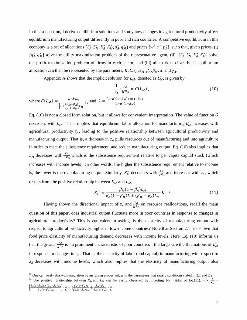
In this subsection, I derive equilibrium solutions and study how changes in agricultural productivity affect

equilibrium manufacturing output differently in poor and rich countries. A competitive equilibrium in this

economy is a set of allocations

and prices , such that, given prices, (i)

solve the utility maximization problem of the representative agent, (ii)

solve

the profit maximization problem of firms in each sector, and (iii) all markets clear. Each equilibrium

allocation can then be represented by the parameters, and .

Appendix A shows that the implicit solution for , denoted as , is given by,

where

and

.

Eq. (10) is not a closed form solution, but it allows for convenient interpretation. The value of function

decreases with .13 This implies that equilibrium labor allocation for manufacturing increases with

agricultural productivity , leading to the positive relationship between agricultural productivity and

manufacturing output. That is, a decrease in pulls resources out of manufacturing and into agriculture

in order to meet the subsistence requirement, and reduce manufacturing output. Eq. (10) also implies that

decreases with

which is the subsistence requirement relative to per capita capital stock (which

increases with income levels). In other words, the higher the subsistence requirement relative to income

is, the lower is the manufacturing output. Similarly, decreases with

and increases with , which

results from the positive relationship between and ,

14

Having shown the directional impact of and

on resource reallocations, recall the main

question of this paper, does industrial output fluctuate more in poor countries in response to changes in

agricultural productivity? This is equivalent to asking, is the elasticity of manufacturing output with

respect to agricultural productivity higher in low-income countries? Note that Section 2.1 has shown that

food price elasticity of manufacturing demand decreases with income levels. Here, Eq. (10) informs us

that the greater

is - a prominent characteristic of poor countries - the larger are the fluctuations of

in response to changes in . That is, the elasticity of labor (and capital) in manufacturing with respect to

decreases with income levels, which also implies that the elasticity of manufacturing output also

13 One can verify this with simulation by assigning proper values to the parameters that satisfy conditions stated in 2.1 and 2.2. 14 The positive relationship between and can be easily observed by inverting both sides of Eq.(11).

9

decreases with income levels. This is a key observation in this model, which leads to higher level of

industrial output volatility in poor countries than in rich ones. The following propositions summarize our

observations on the implicit solutions of the theoretical model.

Proposition 1. Labor and capital move away from manufacturing and into agriculture in response to a

decrease in agricultural productivity. This effect decreases with income levels.

Proposition 2. The elasticity of manufacturing output with respect to agricultural productivity is positive

and decreases with income levels.

In contrast, how does the result differ if we assume the subsistence requirement to be zero?

The utility function then becomes a usual Cobb-Douglas function, and the new general equilibrium

solution for can be obtained using Eq. (10) and as follows:

Note that consumers pay for manufacturing, and Cobb-Douglas production technology implies

that fraction of is spent on labor in manufacturing. Also, fraction of is

spent on labor in agriculture, which justifies Eq. (4). Similarly, equilibrium allocation for capital in

manufacturing is,

Unlike the case with Stone-Geary preferences, we notice that Eqs. (12) and (13) do not involve

productivity terms and . Thus, shocks to agricultural productivity have no effect on manufacturing

output under the assumption of Cobb-Douglas preferences.

In order to illustrate the intuition of the model, Figure 2 presents how equilibrium output changes

in response to a decrease in agricultural productivity using production possibility frontiers (PPF) and

Stone-Geary utility indifference curves. Figure 2 shows that the proportional change in manufacturing

output is larger, when a country’s income is close to subsistence level. The y-axis and x-axis represent the

amounts of agricultural and manufacturing goods, respectively. The outer PPF shrinks vertically to the

inner one in response to a negative shock to agricultural productivity. The top two Stone-Geary

indifference curves that share the ray of origin O1 feature a subsistence requirement that is close to the

income level, while the other two indifference curves with the ray of origin O2 feature a relatively low

subsistence requirement. The equilibrium output occurs at points where the indifference curves and PPFs

are tangent. As for the preferences associated with O1, the equilibrium manufacturing quantity falls from

10

M2 to M1 in response to a decrease in agricultural productivity. Meanwhile, the other two equilibrium

points associated with the low level of subsistence have experienced a decrease in manufacturing from

m2 to m1. From the figure, we notice that

. The change in the PPF in response to a shock to

agricultural productivity is the largest near the y-axis. As a result, the equilibrium points near the location

also experience a large proportional change in manufacturing output, which is possible only when the

country’s income is close to subsistence. In short, the proportional change in manufacturing is large when

the level of subsistence relative to income is high, implying Proposition 2.

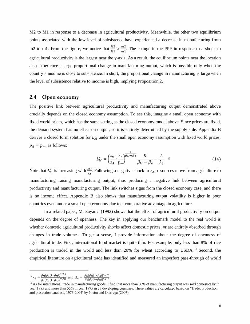
2.4 Open economy

The positive link between agricultural productivity and manufacturing output demonstrated above

crucially depends on the closed economy assumption. To see this, imagine a small open economy with

fixed world prices, which has the same setting as the closed economy model above. Since prices are fixed,

the demand system has no effect on output, so it is entirely determined by the supply side. Appendix B

derives a closed form solution for under the small open economy assumption with fixed world prices,

, as follows:

15

Note that is increasing with

. Following a negative shock to , resources move from agriculture to

manufacturing raising manufacturing output, thus producing a negative link between agricultural

productivity and manufacturing output. The link switches signs from the closed economy case, and there

is no income effect. Appendix B also shows that manufacturing output volatility is higher in poor

countries even under a small open economy due to a comparative advantage in agriculture.

In a related paper, Matsuyama (1992) shows that the effect of agricultural productivity on output

depends on the degree of openness. The key in applying our benchmark model to the real world is

whether domestic agricultural productivity shocks affect domestic prices, or are entirely absorbed through

changes in trade volumes. To get a sense, I provide information about the degree of openness of

agricultural trade. First, international food market is quite thin. For example, only less than 8% of rice

production is traded in the world and less than 20% for wheat according to USDA.16

Second, the

empirical literature on agricultural trade has identified and measured an imperfect pass-through of world

15

and

16 As for international trade in manufacturing goods, I find that more than 80% of manufacturing output was sold domestically in year 1985 and more than 55% in year 1995 in 27 developing countries. These values are calculated based on ‘Trade, production, and protection database, 1976-2004’ by Nicita and Olarrega (2007).

11

food prices to domestic food prices. Countries impose barriers to agricultural trade to protect domestic

markets from international price variability (e.g., Anderson and Nelgen 2012; Gouel 2012; Martin and

Anderson 2012). For example, Anderson and Nelgen (2012) show that the un-weighted average of the

elasticity of international price transmission to domestic markets (for rice, wheat, and maize) was 0.52,

which means that a 1% increase in international prices results in only a 0.52% increase in domestic

prices.17

In short, in the real world with costly trade, a combination of low agricultural trade volumes and

explicit protection of domestic agricultural markets lead to imperfect pass-through of international prices.

Thus, domestic supply and demand play a crucial role in determining equilibrium prices and output. This

is equivalent to saying that the direction of the closed economy results may still hold in an open economy

model with costly trade, but the magnitudes will be attenuated by the presence of international markets

(i.e., rather than food prices rising by 10% in response to a decrease in domestic agricultural productivity,

maybe the food price rise only by 5% in an open economy; see Appendix C, where I extend the model to

allow the partial transmission of international prices). This suggests that the closed economy model can

provide valuable information about the real world.

3 Quantitative analysis

Using the equilibrium solutions of the closed economy model in the previous section, this section

simulates varying effects of agricultural productivity shocks on manufacturing output at different levels of

per capita income. Consistent with the predictions from the previous section, I find that (i) the

proportional change in manufacturing output (and resources used in manufacturing) in response to an

increase in agricultural productivity is positive and decreases with income levels (Propositions 1&2); (ii)

as a result, manufacturing output volatility decreases with the level of income. Note that even though

empirical analysis is provided in the next section, the calibration exercise is also important to understand

the magnitude of the effects implied by the model. Furthermore, the equilibrium solutions of the model

are not closed-form, which makes algebraic comparative statics extremely complex.

3.1 Calibration

Recall that each one of the equilibrium solutions,

is the function of the

parameters, and , whose values need to be assigned for the purpose of simulation.

Labor hour parameter is normalized to 1, and the data on per capita capital stock across countries

17 They use a partial-adjustment geometric distributed lag formulation to estimate elasticities for each key product for 75 countries for the period 1985-2004.

12

come from Weil Lab Data (2011). for each country is normalized by the per capita capital stock of

Ethiopia. Ethiopia is chosen to be a base country, as it is one of the poorest countries in UNIDO (2011)

manufacturing data, and its per capita income is close to the lower poverty line ($275 in 1990 US dollars)

proposed by World Bank (1990).18

The manufacturing production parameter , the capital income share

in manufacturing, comes from the GTAP (2007) input-output table of India and is set to 0.58.19

The

capital income share in agriculture is set to 0.32 according to the same input-output table of India. The

yearly values of for each country are set at each country’s annual cereal yields (measured as kilograms

per hectare of harvested land, includes wheat, rice, maize, etc.; taken from FAO) for the period 1970-

2002 and are normalized by Ethiopia’s minimum cereal yield which is 974kg/hectare. The time-varying

cross-country values of range from 1 to 7.64. For example, the average (during 1970-2002) for the

U.S. is about 4.5, which implies that agricultural productivity in the U.S. is more than four times as high

as Ethiopia’s. Meanwhile, is set to be a free parameter that matches each country’s income from

agriculture and manufacturing. for Ethiopia is normalized to 1, and for other countries are set at

those values so that the incomes implied by the benchmark model are the same as the income data

normalized by Ethiopia’s income level.

The preference parameters, utility weight and the subsistence requirement , are calculated

using data on the employment shares for the U.S. and Ethiopia (note that these parameters are common to

all countries and all time periods). The share of employment in manufacturing, out of the sum of

employment in agriculture and manufacturing, for the U.S. in year 2004 is 0.91. I plug this number back

in in Eq. (12) and solve for , which results in .20

Recall that Eq. (12) is the equilibrium

solution of when . Although we have in our benchmark model that features the Cobb-

Douglas Stone-Geary utility function, the corresponding equilibrium solution Eq. (10) approaches Eq.

(12) as the subsistence relative to income

approaches zero. We assume that it is small enough in the

U.S. such that Eq. (12) is roughly the same as Eq. (10), which gives us the approximate value of for the

Stone-Geary preferences. Actually, in Stone-Geary preferences can also be interpreted as the food

expenditure share, when subsistence relative to income is negligible. Hence, one can also use data on food

expenditure shares directly instead of employment shares, but the problem is that food expenditure data

suffer from inconsistent definitions of food consumption such as food away from home, which includes

service. For this reason, I use employment data to calibrate utility parameters. Similarly, is obtained by

18 Defining the poorest country is important in this model with preferences featuring a subsistent requirement in order to avoid corner solutions. All other parameter values are assigned in a way that it ensures interior solutions for all countries. 19 Capital income share in manufacturing is calculated as the ratio of the value of capital stock used in manufacturing sectors to the sum of capital stock value and labor compensation value from the I-O table. 20 This is a typical way of assigning a value to the parameter in structural change literature. For example, see Restuccia, Yang, and Zhu (2008).

13

plugging the share of employment in manufacturing for Ethiopia, which is 0.07 in 2004, in Eq. (10),

which leads to . To summarize, Table 2 presents the calibrated parameter values and data

source.

3.2 Quantitative results

In this section, I present the results of simulations of the model based on the calibrated parameter

values. For each country in the sample, I compute its yearly equilibrium manufacturing output, output

growth rates, and the standard deviation of the growth rates (volatility). The key questions are: (i) how

does a change in affect the proportional change in equilibrium manufacturing output differently across

countries depending on the level of per capita income?; (ii) what are the quantitative predictions about

volatility in response to shocks to agricultural productivity?

Column 1 in Table 3 reports per capita capital stocks normalized by Ethiopia’s, and column 2

reports country-specific average crop yields over the period 1970 – 2002, denoted as . We see that

the per capita capital stock and the average crop yield (a proxy for agricultural productivity) roughly

increase with countries’ per capita income levels. With these country-specific values for and ,

equilibrium solutions are simulated when and when

. In other words, each

equilibrium is computed at average levels of productivity and at 10% higher levels. For example,

Ethiopia’s average yield is 1.20 which is used in columns 3 – 6 (in the first row), and 1.1 * 1.20 = 1.32 is

used in columns 7 and 8.

Column 3 of Table 3 reports subsistence consumption relative to income implied by the model

when

decreases with income levels from 0.77 (for Ethiopia) to 0.04 (for the U.S.),

consistent with the fact that a large fraction of income is spent on food in Ethiopia while subsistence

consumption matters significantly less in the U.S. Due to the large share of income used to meet the

subsistence requirement, in Ethiopia, a rise of causes a significant reallocation of labor. The share of

labor used in manufacturing rises from 0.15 to 0.20 when increases by 10%, as shown in columns 4

and 6. This leads to a large change (a 29% increase) in manufacturing output.

This seemingly counterintuitive result (labor flows away from the sector with rising productivity)

is due to subsistence requirements in agriculture. When these requirements are small relative to income,

the reallocation is much smaller. For example, in the U.S. the same shock to agricultural productivity

causes the manufacturing output to change only by a factor of 1.004. In short, in response to a positive

shock to agricultural productivity, changes in manufacturing output and resources decrease with income

levels.

14

Table 3 confirmed the Propositions 1 and 2 that elasticities of manufacturing output and labor and

capital used in manufacturing are positive and decrease with income levels. This also implies that the

degree of fluctuations in manufacturing output in response to shocks to agricultural productivity will be

higher in poor countries. Indeed, this is confirmed in Table 4, which reports simulation results on

volatility which is the standard deviation of implied industrial output growth rates over the period 1970-

2002.21

Column 1 in Table 4 reports volatilities of simulated manufacturing output growth rates for each

country (here, is set at the original country specific time-varying crop yields). We see that poor

countries exhibit much higher level of output fluctuations compared to rich countries. For example, the

volatility is about 37.5% for Ethiopia, while it is 0.6% for the U.S. Column 2 displays the standard

deviation of yearly proportional changes in crop yield (yield volatility). Countries that have larger shocks

to agriculture are subject to higher industrial output volatility. For example, even if Portugal is richer than

Bangladesh, Portugal’s implied volatility is slightly higher because crop yield volatility is three times

higher in Portugal than in Bangladesh (It is also partially due to the lower agricultural productivity in

Portugal; as shown in Table 3, the average yield in Portugal is 1.77 while it is 2.36 in Bangladesh).

In order to see volatility patterns after controlling for the size of the shocks, I build common

shocks for all countries by drawing thirty-three times independently from the truncated normal

distribution . This can be considered as rainfall shocks that are common to all countries.

Since the level of agricultural productivity differs across countries, I multiply each by each country’s

average crop yield . Manufacturing output values are then simulated for each country, and the

computed volatilities are reported in column 3 of Table 4. We see that the volatility is monotonically

decreasing in income levels even with the equivalently sized shocks to productivity. Note that if we have

assumed CES Stone-Geary preferences instead of Cobb-Douglas Stone-Geary, the pattern of volatility

against income levels will be U-shaped, as shown in Figure 3. The volatility decreases as income effects

wear off, and starts increasing again when substitution effects become dominant (this case is fully worked

out in Appendix C). The last column in Table 4 displays real manufacturing output volatilities calculated

using UNIDO (2011) manufacturing output (value added) data for the period 1970 – 2002. Consistent

with the theory, in poor countries the implied volatility caused by fluctuations in crop yield tend to

explain a large fraction of the real output volatility. In sum, this simulation exercise helps understand the

mechanisms of the proposed theory and provides a good sense about differing extents to which

agricultural productivity shocks affects volatility across countries with varying levels of per capita

income.

21 Note that the values of output volatility are presented in percentage terms to give a better sense about for the impacts. To illustrate, if a country experiences output growth equal to 1.03, we say that the country’s output grew by 3%. Thus, reporting a country’s output volatility as 37.5% - as an example for Ethiopia – is more intuitive than reporting it as 0.375.

15

3.3 Discussion

The quantitative implementation of the theory potentially bears two concerns: (i) the existence of

international trade may weaken the income effect. As an example, we saw that in a small open economy,

the effect of a shock to agricultural productivity changes signs; (ii) the data on crop yields might be

subject to endogeneity. In order to address the former issue, Appendix C shows how the world food

market affects domestic food prices and presents results on modified calibration exercises in which

shocks to domestic agriculture supply affect domestic food prices only partially. As for the endogeneity

issue, note that crop yields, measured as production quantity per unit of land, also depend on labor and

capital that are used in agriculture. Thus, shocks to the resource supply (e.g., agriculture subsidies and

trade liberalization) may lead to endogenous changes in resource allocation, which results in changes in

both manufacturing output and crop yields. The following section addresses these issues and

complements the theoretical results with instrumental variable regression analysis using data on

manufacturing sectors across countries.

4 Empirical strategy and data

4.1 Empirical Strategy: instrumental variable approach

The theory suggests that a decrease in agricultural productivity shifts resources away from manufacturing

and into agriculture, thus reducing manufacturing output (positive link between agricultural productivity

and manufacturing output). This effect is larger when a country’s income level is low, causing larger

output declines in poor countries. To test these predictions, we need exogenous movements in agricultural

productivity that vary across countries and time. I use crop yield as a proxy for agricultural productivity,

and capture exogenous variation in yields using shocks to rainfall.

The unit of observation is a country in a given year , and the main estimating equation is as

follows:

where is manufacturing output in country in year ; denotes crop yield in country in year

, a proxy for agricultural productivity; is a country fixed effect which captures country specific time

trends of manufacturing output such as technological progress; is an idiosyncratic error term.22

Estimating the model in first-differences simplifies the framework by eliminating country specific and

time invariant effects (e.g., land quality, climate conditions, and industry composition of the country). I

22 I exclude manufacturing sectors that use agricultural products as intermediate inputs (such as food, tobacco, and cotton) in empirical analysis at the aggregated level to avoid the direct consequences of the shocks to agriculture on manufacturing.

16

test whether the coefficient or is significantly positive and whether the effect is larger in poor

countries than in rich ones. While the best way is to include income level interacted with yield growth,

this is avoided due to sample size and multicollinearity with other variables such as financial development

(more details appear below). Importantly, the estimation framework (15) exactly resembles the calibration

exercise associated with Table 3 (where we examined proportional changes in manufacturing output in

response to a 10% increase in ), although it is reduced-form estimation. In addition, I include the lagged

yield growth in Eq. (15) in order to allow a time lag between an agricultural shock and its impact on

manufacturing – for example, in a upper-hemisphere country where the harvest occurs in the fall, the

effect of the shock on the manufacturing can be shown in the data of the following year.

An important concern in estimating Eq. (15) is that crop yields and industrial output can be

determined by factors outside the model, leading to bias in the estimate effect. Consider two examples.

First, suppose there is common technological progress that raises productivity in all sectors of the

economy. This will generate a positive correlation between crop yields and industrial output independent

of the mechanism in this model. Second, crop yield (output per unit of land) is used as a measure of

agricultural productivity because it is consistently available for many countries and time periods. Crop

yields differ from a pure total factor productivity (TFP) measure because yields depend on the amount of

resources such as labor and capital used in agriculture. Since agriculture and manufacturing compete for

resources, changes in policies that favor one sector will induce a negative correlation between crop yields

and manufacturing output. For example, when a government decides to subsidize agriculture, this pulls

resources out of manufacturing and into agriculture, reducing manufacturing output and raising crop

yields at the same time. This generates downward bias in OLS results in Eq. (15).

The solution for both cases is to find a source of exogenous variation in agricultural TFP.

Detailed studies of crop yields show that yields are sensitive to changes in rainfall and changes in

temperature (e.g., Lobell et al. 2007; Schlenker et al. 2009). I use rainfall shocks, as previous studies

argue that heat directly affects manufacturing workers’ productivity (West 2003; Chen 2003; Chan 2009).

The first-stage relationship between crop yield and rainfall is as follows:

where is country fixed effect; includes rainfall growth rates at time and interacted with

tropical region dummy (equal to 1 if a country is in a tropical region); is the error term. In the

17

estimation of Eq. (15), rainfall growth rates at time and and interaction variables serve as

instruments for the endogenous regressors,

and

.

23

The theory suggests that the main channel through which changes in agricultural productivity

affect manufacturing output is the reallocation of labor and capital between the two sectors (Proposition

1). Using data on employment in manufacturing, gross capital investment in manufacturing and the area

of land under cereal production, I test the prediction using similar frameworks:

where ,

and are the number of employees in manufacturing, capital investment in

manufacturing and agricultural land in country in year ; is a country fixed effect. Eq. (16) again

serves as a first-stage estimation framework.

Recall that this paper introduced a relatively simple general equilibrium model with Stone-Geary

preferences, which does not incorporate some features that may be important to other studies. For

example, if a country has a well-developed financial system, the effect of agricultural shocks on resource

reallocation may decline because each sector can hedge against economic shocks by savings and

borrowings. I test how the level of financial development affects the extent to which agricultural shocks

impact manufacturing, using data on private credit provided by banks and other financial institutions

according to Levine et al. (2000). The best way to test this is to include the financial development

measure interacted with yield growth in the estimating equation. However, financial development is

correlated with several other variables such as per capita income level and the share of agriculture

production, and they all significantly affect the extent to which agricultural shocks impact manufacturing.

Given that the number of countries in the sample is just around 100 with less than 2000 observations in

total, including all those relevant measures leads to multicollinearity. Thus, I test the predictions by

restricting the sample to countries at different levels of per capita income, the measure of financial

development, the share of agricultural production, and openness to trade. Then I compare the coefficients

on yield growth.

23 Jayachandran (2006) also uses crop yield as a proxy for agricultural TFP and rainfall shocks to instrument crop yields in order to study changes in agricultural wages in response to productivity shocks. Miguel et al. (2004) uses rainfall growth to instrument income growth in African countries and study the effect of economic conditions on the likelihood of civil conflicts. Dercon (2004) uses panel data from rural Ethiopia and rainfall shocks in order to study consumption growth.

18

4.2 Data

Data on industry-level annual value added, employment, and gross capital investment come from the

2011 UNIDO Industrial Statistics Database. I use INDSTAT2 that reports data according to the two-digit

ISIC Revision 3 classification for the period 1970 – 2002.24

Although the original UNIDO data set

contains 23 sectors, I aggregate those sectors into 8 categories for two reasons. First, many countries

(especially, low-income countries) report values that are aggregated from multiple sectors (for example,

some countries combine metals and machinery together and report as metals). Second, sectors with

similar characteristics are grouped into the same category, and such level of disaggregation (8 categories)

is enough for studying sector specific effects of agricultural productivity on manufacturing output, capital

investment, and employment. The list of sectors is displayed in Table 5. Sector 1, which includes food

and tobacco, is excluded in every regression, as it is directly related to agriculture and not of interest.

Sector 2 which is associated with textile industries is also excluded in aggregate-level regressions since

agricultural products such as cotton might be intensively used as a primary input (I also report results of

this sector in sector-specific analysis).

Precipitation data for the period 1970 – 2002 are taken from United Nations Environment

Programme (UNEP). This dataset reports worldwide annual precipitation at 0.5 0.5 degree resolution

(approximately 56km 56km at the equator).25

The crop distribution data are taken from Agricultural

Lands in the Year 2000, Ramankutty et al. (2008). This dataset contains the distribution of global

agricultural lands in the year 2000 at 5-minute resolution in latitude by longitude (approximately 7km

7km), which I aggregate this to match with the precipitation data at 0.5 0.5 degree resolution. In this data

set, each data point is assigned a value ranging from zero to one, where the value is zero if there is no

crops are grown in the area and is 1 if the area is completely covered in crops. I use Geographic

Information Systems (GIS) software to aggregate the precipitation data to the country-year level,

weighting by the crop distribution. This accurately captures the amount of rainfall that is relevant to

agricultural land in each country.26

The available measure of agricultural productivity is cereal yield, the crop weight (kilograms)

produced per unit (hectare) of harvested land. The cereal yield data come from FAO and include major

24 The original dataset goes from 1963 to 2009. But the data used employed in this paper stops at 2003 because of the unprecedented food crisis that happened in recent years. International food prices started increasing rapidly in 2004 due to the increasing demand for bio-fuels. Accordingly, countries started imposing severe restrictions on food exports, which lead to 2007-8 food crisis. 25 According to UNEP, “the original data took the form of a value for each month and each box on a 0.5 degree latitude/longitude grid. The annual values are the average of their constituent months, which have been calculated by GRID-Geneva. Original Data

Station observations were first collected by national meteorological and related data. These observations were gridded by collaborators at the Climatic Research Unit (www.cru.uea.ac.uk).” 26 Other economic studies related to agriculture use rainfall data weighted by the population distribution or un-weighted rainfall data (e.g. Bastos et al. 2013; Miguel et al. 2004).

19

staple crops such as wheat, rice, maize, barley, oats, rye, millet, etc. The following four datasets are taken

from World bank data set: the share of agricultural value added as a share of GDP, aggregate private

credit provided by banks and other financial institutions as a share of GDP, and land under cereal

production. Note that, consistent with Levine et al. (2000), the second dataset is used as a measure of

financial development. The first two data sets, the share of agriculture and private credit, are used to

estimate the differing effects of shocks to agricultural productivity on manufacturing output depending on

those conditions. Additionally, I use yearly data on the area of land under cereal production in

conjunction with the data on resources in manufacturing in order to forecast the resource movement

between manufacturing and agriculture in response to changes in agricultural productivity. To summarize,

Table 6 presents descriptive statistics for the data used in regression analysis.

5 Empirical results

5.1 Rainfall and crop yield (first-stage)

Table 7 shows the first-stage relationship between yearly log growth rates in crop yield and rainfall.

Column 1 reports the estimates when the sample of countries is restricted by per capita income below

$4,000. A 1% increase in rainfall in current year leads to a 0.33% increase in crop yield in current year

(the t-statistic of the estimate is 11.06). To control for differing effects of rainfall in tropical and non-

tropical countries, I include a tropical region dummy – which is 1 if a country is in a tropical region –

interacted with the rainfall growth. Its estimated coefficient is -0.28 and is significant at the 1% level,

which implies that a tropical climate reduces the impact of rainfall on yield by more than 80%.

Meanwhile, rainfall growth in previous year registers insignificantly. Column 2 shows that the regression

result is highly robust to the inclusion of country fixed effects. In addition, in order to examine the

possible effect of excessive rainfall, I construct a dummy that takes 1 if rainfall in the previous year

exceeds the average rainfall over the period 1970-2002. The result in column 3 shows that excess rain

interacted with rainfall growth registers insignificantly. This implies that outside tropical regions, positive

rainfall growth tends to lead to higher crop yields.

Columns 4 and 5 in Table 7 report regression results with and without fixed effects for countries

with income below $10,000. The coefficients on log rainfall growth are about 0.28, which fell by about

15% while the levels of t-statistic slightly rose, compared to the estimates in the first two columns. When

the per capita income level is restricted between $10,000 and $20,000, the coefficient drops even more to

0.10 while it is still significant at the 1% level (column 7, tropical region interaction terms are not

included as there are no high-income countries in those regions). This implies that the effect of rainfall on

crop yields decreases with a country’s level of economic development, which might be attributable to

20

better irrigation system in developed countries. The F-statistic for high-income country sample is 7.30,

which is reasonably high (generally, a value greater than 10 is considered to be an indication for strong

instruments), but IV-2SLS estimates may be somewhat biased toward OLS estimates. However, we see

that the F-statistics in columns 1-6 are all greater than 36, implying that rainfall instruments are strong.

For the

5.2 Manufacturing output and agricultural productivity (second-stage)

Table 8 presents results of the second-stage estimation on Eq. (15) which is the relationship between log

growth in manufacturing output (value-added) and log growth in crop yield. Column 1 reports OLS

results for countries with per capita income less than $4,000 (in 2005 international dollars). The

coefficient on lagged log growth in cereal yield, which represents the elasticity of manufacturing output

with respect to crop yield, is 0.09. Meanwhile, the 2SLS-IV result on the same coefficient is 0.38 and

significant at the 5% level (column 2), implying that a 1% exogenous increase in crop yield in the

previous year leads to a 0.38% increase in current year manufacturing output for developing countries.

Both results indicate that an increase in agricultural productivity increases manufacturing output

(consistent with Proposition 2), but the magnitude of the OLS result is smaller than the 2SLS-IV result.

As discussed in section 4.1, the fact that manufacturing and agriculture compete for the same resources in

a country can result in a negative correlation between crop yield and manufacturing output, as yield

(output per unit of land) depends on the amount of resources that are used. This makes yield endogenous,

leading to downward bias of the OLS results.

In order to test whether the effect is reduced for higher-income countries, I raise the income cut-

off to $10,000 and find that the 2SLS-IV result on lagged yield growth is 0.33 (column 5) – 0.05 point

less than the coefficient with $4,000 income cut.27

Furthermore, when the sample is restricted to per

capita incomes between $10,000 and $20,000, the estimated effect of yield on manufacturing output turns

out to be insignificant (column 7). These results support Proposition 2 of the theory that the income effect

caused by agricultural shocks on manufacturing volatility wears off as a country becomes richer. In

addition, note that in Table 8 most of the coefficients on lagged yield growth are significantly positive,

while the current yield growth registers insignificantly. As mentioned in section 4.1, a plausible reason

may relate to agricultural seasonality – especially for upper hemisphere countries – and a time lag

between an agricultural shock and its impact on manufacturing.

27 As discussed in section 4.1, I run separate regressions with different income cuts rather than including interaction variables due to multicollnearity problem associated with highly but not perfectly correlated covariates such as the measure of financial development or the share of agriculture.

21

In the theoretical model the key mechanism that causes the link between agricultural productivity

and manufacturing output was resource reallocations between the two sectors. Because the model

assumes no saving and borrowing, the only way to compensate for a negative shock to agriculture – in the

presence of subsistence requirements – is to pull resources away from manufacturing and into agriculture.

Thus, if one can show that the effect of agricultural productivity shocks on manufacturing is larger in

countries with underdeveloped financial systems, the key argument of the theory is strengthened. Indeed,

when the sample is further restricted to the countries with private credit less than 30% of GDP – this is

quite low considering that 80% is the average level for countries with per capita income greater than

$10,000 – and per capita income less than $10,000, the 2SLS-IV result on lagged yield growth jumps to

0.43 at the 5% level significance (see column 3 in Table 9). The estimated value is even larger than the

estimated coefficient when the income cut-off is $4,000, which was 0.31 (column 1). Note that the

average per capita income of the sample in column 3 in Table 9 is almost twice as large as the one in

column 1. This suggests that a country’s financial system plays an important role in predicting the effects

of agricultural shocks on manufacturing volatility. In column 5, the regression additionally restricts the

sample to countries with the share of agriculture to GDP larger than 20%. The estimated coefficient

becomes even larger, 0.47, and is significant at the 1% level. In fact, this result is anticipated by the

theory that if a country has a comparative advantage in agriculture then the effect of agricultural shocks

on manufacturing is large, as agricultural shocks matter more in those countries.

5.3 Resource reallocations and agricultural productivity (second-stage)

Recall that the theory predicts that in poor countries a negative shock to agricultural productivity pulls

resources away from manufacturing and into agriculture in order to meet food subsistence requirements.

Having shown the estimated effects of crop yield on manufacturing output, we now examine the specific

resource channel, using yearly data on the number of employees, gross capital investment in

manufacturing, and land area under cereal production.

Employment in manufacturing

Table 10 reports estimation of Eq. (17), in which I regress log growth in manufacturing

employment on growth rates in crop yield, while varying the minimum latitude in order to take

agricultural seasonality into account. The seasonality consideration is important in examining labor

movements between agriculture and manufacturing, since unlike other inputs labor mobility is especially

limited by time, space and willingness to migrate. As an example, an agricultural worker in a country in

the upper-hemisphere (away from the equator) has higher incentive to move to other sectors after the

harvest in the fall, since there is not much work to do during the winter or probably until the next harvest

22

begins.28

Column 3 in Table 10 shows IV-2SLS results of a regression performed over a subset of

countries (with income below $10,000) that are located above the 10-degrees latitude north. Unlike other

regression results, it is the coefficient on current yield growth that is significantly positive (at the 1%

level), while the coefficient on lagged yield is near zero. The result implies that a 1% increase in cereal

yield in the current year leads to a 0.21% increase in the number of employees in manufacturing the same

year. When the minimum latitude cut is set at 0-degrees, i.e. the equator, the coefficient on current yield

growth decreases from 0.21 to 0.16 (column 4). And, the coefficient further falls to 0.08 (column 5) when

all countries (with per capita income below $10,000) are included in the sample. Interestingly, as shown

in column 6, the yield effect on employment becomes significantly larger when the maximum income cut

is lowered to $4,000 (it increased from 0.20 to 0.28 with the 1% level of significance). A plausible

explanation for this phenomenon is that workers are more willing to move across sectors when they are

extremely poor.

A question to ask is, why does current year yield growth have significant effects

on manufacturing employment growth while the effect of lagged yield growth

is close to zero? In the northern hemisphere countries, when there is a positive shock to yield,

manufacturing demand rises due to income effects, and workers can move out of agricultural fields to

work in manufacturing after the harvest in the fall. For simplicity, assume that ten people work in

manufacturing each year when there is no shock to yield. Also, suppose that a positive shock to yield

occurred in year and one worker moved from agriculture to manufacturing after the harvest in the same

year and continue to work in the industry until the next year before the next harvest. Now, the number

of employees in manufacturing is 11 both in and , while it is still 10 at time . Thus, log

employment growth is log(11/10) at time while it is log(11/11) = 0 at time . Basically, the positive

agricultural shock occurred in year appears to affect the employment growth in year positively, while

the same shock in year has zero effect on the employment growth in year . Thus, this example

explains why the coefficients on current yield growth are significantly positive while the coefficients on

lagged yield growth are close to zero.

Table 11 displays sector-specific regression results. Interestingly, the last two sectors – highly

capital-intensive industries such as electrical machinery and motor vehicles – appear to register

insignificantly. A plausible explanation is that capital-intensive industries are more willing to keep

workers from moving to other sectors, because costly capital assets need to be operated continuously to

28 Postel-Vinay (1994) discusses mobile temporary workers in eighteenth century France as follows: “… every summer thousands of industrial workers left their jobs to work in the grain fields. … Wheat production expanded most in districts where

industrial workers were temporarily available for harvest work…” Given the existence of mobile temporary workers in the eighteenth century, it might be reasonable to expect something similar in developing countries today since transportation and communication technology makes matching between temporary workers and jobs easier. Plus, the willingness for temporary migration for any kind of jobs increases with a worker’s poverty.

23

cover the cost.29

In contrast, other sectors that are relatively more labor-intensive such as wood products

display significant effects of exogenous shocks to yield on manufacturing employment (columns 2-6).

Employment in textiles, on the other hand, appears to be less responsive to changes in yield despite its

labor intensiveness, which might be due to heavy dependence on exports.

Capital investment in manufacturing

Table 12 reports estimation results of Eq. (18), in which I examine the effects of changes in

agricultural productivity on gross capital formation in manufacturing. The 2SLS-IV result in column 2

indicates that a 1% increase in lagged and current yields leads to 1.68% and 1.89% increases in capital

investment in manufacturing, respectively (for observations with per capita income less than $10,000).

Note that both coefficients on lagged and current yield growth are significantly positive, while

manufacturing employment growth appeared to be responsive only to lagged yield growth. This might be

because capital can be invested anytime when there is demand due to less restriction on mobility

compared to labor.

Table 13 shows sector-specific regression results on gross capital formation in manufacturing. I

find that capital investment in relatively more capital-intensive sectors (such as motor vehicles and

electrical machinery) is highly responsive to changes in yield. In contrast, industries related to wood

products (sector 3), which tend to be labor intensive, registers insignificantly. Interestingly, as shown in

Table 11, these results flip when it comes to employment: wood product sector employment was highly

responsive to exogenous changes in yield, while motor vehicle and electrical machinery sectors were not.

This shows that factor intensity of manufacturing sectors matter when it comes to factor-specific response

to agricultural shocks.

Resources in agriculture

Having empirically shown the effect of exogenous shocks to yield on resources in manufacturing,

now we examine the effect of the shocks on resources in agriculture. Table 14 shows 2SLS-IV results of

the relationship between land under cereal production and crop yields. I find that the coefficients on

lagged yield growth are negative and significant at the 5% level (columns 2 and 3). This countercyclical

relationship between agricultural productivity and resources in agriculture is implied by the theory. For

example, if a country experiences a drought in the previous year it expands agricultural land the next year

due to the increased profitability caused by food price increases. Note that, unlike most regressions that

29 This phenomenon also existed in eighteenth century France, and Potel-Vinay (1994) notes with another explanation that “…

many new technologies involved costly investments that needed to be continuously operated to cover their cost. Firms intending to introduce new techniques thus had to raise wages to hold workers through the peak summer season in order to develop an experienced workforce.”

24

are performed over the sample with per capita income below $10,000 or $4,000, the regressions in Table

13 are performed over the sample excluding low-income countries. This is because data on harvested land

are collected by survey, and it is unlikely for poor countries’ data to be informative enough for tracking

subtle yearly changes in land use. This is because the majority of the agricultural fields in poor countries

are privately managed by individuals or families. Nonetheless, I argue that the regression results in Table

13 can be reasonably applied to poor countries. When an adverse shock to crop yield is experienced in the

previous year, relative food prices increase even more in poor countries than in rich ones due to the

subsistence requirement. This gives poor countries a high incentive to invest more in land development

the next year.

5.4 Fluctuations in predicted manufacturing output growth

Table 15 reports standard deviations of predicted manufacturing output growth rates based on the 2SLS-

IV estimation results of Eq. (15) for selected developing countries. Given rainfall data, predicted yield

growth rates are obtained from the first-stage analysis. In the second stage, we can then predict

manufacturing output growth using the first-stage result. Column 1 in Table 15 reports volatilities of the

predicted manufacturing output growth rates, and the average value of such volatilities for the developing

countries is found to be 5.91%. The real manufacturing output volatilities calculated directly from the

data are also presented in column 2, which shows that the average volatility for developing countries is

29.25%. The values in column 3 are obtained simply by dividing volatility of predicted output growth

(column 1) by the real volatility (column 2). The average of such ratios for 44 developing countries is

0.28, which suggests that rainfall shocks to crop yield can explain about 28% of manufacturing output

fluctuations in developing countries.

Let us finish this section with a summary of the empirical findings. Consistent with the

simulation results, I find that the estimated manufacturing output elasticity with respect to agricultural

productivity is significantly positive for developing countries, and it becomes insignificant for high-

income countries. Additionally, I find that the elasticity is larger when a country is financially

underdeveloped and when the share of agriculture in GDP is high, which corroborates the suggested

mechanism. Moreover, the results also show strong evidence for the channel proposed in the theory: (i) a

decrease in agricultural productivity decreases both capital investment in manufacturing and employment

in manufacturing in developing countries; (ii) a decrease in agricultural productivity in the current year

increases land under cereal production the next year. This supports the argument that resources are pulled

out of manufacturing and into agriculture to meet subsistence requirements in response to a negative

shock to agricultural productivity. Finally, by calculating variability of predicted manufacturing output

25

growth based on the estimation results, I find that rainfall shocks to crop yield can account for a

significant fraction of actual manufacturing output volatility.

6. Conclusion

The existing literature attempts to explain why growth rates in industrial output fluctuate more in

developing countries, by focusing on shocks to the supply side of manufacturing and emphasizing

differences in the size of these shocks across countries. Empirically, however, it is difficult to identify and

measure the shocks. Consequently, there is no consensus on whether firms in poor countries are subject to

larger shocks than firms in rich countries.

In contrast, this paper develops a general equilibrium model in which agricultural productivity

shocks are transmitted to industrial output. A key feature is the inclusion of Stone-Geary preferences with

minimum consumption requirements for food. In this environment, adverse shocks to agricultural

productivity require that increased resources be devoted to agriculture to meet subsistence consumption

levels. Resources available to manufacturing fall, as does manufacturing output. Both the calibration

exercise and the empirical analysis show that the strength of the positive link between agricultural

productivity and manufacturing output decreases with income levels, and that the degree of output

fluctuation in response to shocks to agricultural productivity also decreases with income levels.

These findings have important implications for development. First, this paper argues that adverse

shocks to agriculture add considerable uncertainty to manufacturing sectors in developing countries, a

feature which may push investors away and dampen the growth of the economy. Second, subsistence

requirements lead to a perverse counterintuitive situation: resources flow toward the sector with declining

productivity. This sharply curtails the economy’s output and total factor productivity. Therefore,

mitigating the impact of agricultural productivity shocks is a first-order issue for poor countries.

Fortunately, the model suggests a clear solution. A reliable world market for food can help lessen

the impact of agricultural shocks on developing economies. Openness to world trade breaks the link

between domestic productivity and domestic prices. This paper also shows that, in a small open economy,

resources can move to any sector that has become relatively more productive even in the presence of

subsistence consumption. Thus, an economic loss caused by a decrease in agricultural productivity is not

only limited within agriculture but also partly compensated by producing more manufacturing goods.

This implication for international food trade is especially relevant in light of recent developments.

First, climate changes are likely to increase the frequency and severity of droughts (Quiggin 2007; Cline

2008; Lee 2009). Unfortunately, the damages will be the most severe in developing countries, because

they are predominantly located closer to the equator and are already near the thresholds at which further

increases in temperature will reduce agricultural productivity. Second, world leaders are responding to

26

food price shocks by becoming less open to agricultural trade, not more. For example, during the 2007-

2008 world food crisis international prices for rice increased by 160% between 2007 and 2008. In

response, countries tried to insulate their markets from the crisis, restricting food exports, and relying on

storage and self-sufficiency. This paper suggests that such policies are likely to increase industrial output

fluctuations in poor countries caused by agricultural shocks and sheds light on the importance of re-

establishing a reliable world market for food.

Figures and Tables

Figure 1. Aggregate volatility and per capita GDP - standard deviations of per capita GDP growth rates (1970-2002) are plotted against levels of per capita GDP.

27

Figure 2. Changes in equilibrium quantities and a negative shock to agricultural productivity – The production possibility frontier (PPF) contracts vertically in response to a reduction in agricultural productivity. The top two indifference curves are associated with the amount of subsistence requirements close to the income level, representing poor country conditions. The proportional change in manufacturing output is larger for the preferences associated with food subsistence 1 than for the preferences associated with food subsistence 2.

Figure 3. Manufacturing output volatility and per capita capital stock – Equilibrium manufacturing output volatilities are plotted against per capita capital stock under different types of preferences. The same series of agricultural

productivities are applied at each from 20 to 1000 ( less than 20 are omitted for a graphing purpose). [Note: here,

is temporarily assumed as the Matlab had problems solving the implicit solutions for CES preference cases. This will be fixed later, but

the general shape of the above graphs should be the same regardless of the two production function parameter values.]

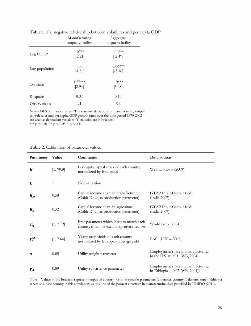
28

Table 1: The negative relationship between volatilities and per capita GDP

Manufacturing output volatility

Aggregate output volatility

Log PGDP -.07** [-2.21]

-.006** [-2.49]

Log population -.03

[-1.56] -.006*** [-3.16]

Constant 1.37*** [2.94]

.19*** [5.28]

R-square 0.07 0.15

Observations 91 91

Note - OLS estimation results. The standard deviations of manufacturing output growth rates and per capita GDP growth rates over the time period 1970-2002 are used as dependent variables. T-statistics are in brackets. *** p < 0.01, ** p < 0.05, * p < 0.1.

Table 2: Calibration of parameter values

Parameter Value Comments Data source

[1, 90.8] Per capita capital stock of each country normalized by Ethiopia’s

Weil Lab Data (2009)

1 Normalization

0.58 Capital income share in manufacturing (Cobb-Douglas production parameter)

GTAP Input-Output table (India 2007)

0.32 Capital income share in agriculture (Cobb-Douglas production parameter)

GTAP Input-Output table (India 2007)

[1, 2.12]

Free parameter which is set to match each country’s income excluding service sectors

World Bank (2004)

[1, 7.64] Yearly crop yields of each country normalized by Ethiopia’s average yield

FAO (1970 – 2002)

0.05 Utility weight parameter Employment share in manufacturing in the U.S. = 0.91 (WB, 2004)

0.89 Utility subsistence parameter Employment share in manufacturing in Ethiopia = 0.07 (WB, 2004))

Note – Values in the brackets represent ranges of country- or time-specific parameters ( denotes country, denotes time). Ethiopia serves as a base country in this simulation, as it is one of the poorest countries in manufacturing data provided by UNIDO (2011).

29

Table 3: Proportional changes in manufacturing output in response to a 10% change in agricultural productivity (simulation results)

Country

Ethiopia 1.00 1.20 0.77 0.15 0.25 0.20 0.32 1.29

Ghana 3.00 1.04 0.63 0.25 0.72 0.30 0.83 1.15

Malawi 2.14 1.19 0.61 0.26 0.62 0.31 0.70 1.14

Uganda 1.28 1.43 0.59 0.28 0.48

0.33 0.54 1.13

India 6.17 1.73 0.29 0.56 1.97 0.59 2.05 1.04

Bangladesh 2.84 2.36 0.27 0.58 1.30 0.61 1.34 1.03

Portugal 60.76 1.77 0.14 0.73 8.92 0.75 9.04 1.02

United States

90.84 4.59 0.04 0.85 12.41 0.86 12.46 1.004

Note – denotes a country-specific average value of cereal yields over the period 1970-2002.

Table 4: Simulated manufacturing output volatility

Country Simulated volatility (country specific

shocks, crop yields) Yield volatility

Simulated volatility (common shocks)

Real manufacturing output volatility

Ethiopia 37.25% 12.15% 30.17% 17.82%

Ghana 19.92% 18.88% 18.47% 42.98%

Malawi 35.03% 44.95% 17.31% 16.47%

Uganda 15.67% 13.61% 16.29% 30.87%

India 3.70% 6.33% 5.50% 10.91%

Bangladesh 2.37% 5.49% 4.95% 24.91%

Portugal 3.07% 16.28% 2.28% 15.13%

United States 0.6% 13.37% 0.7% 6.09%

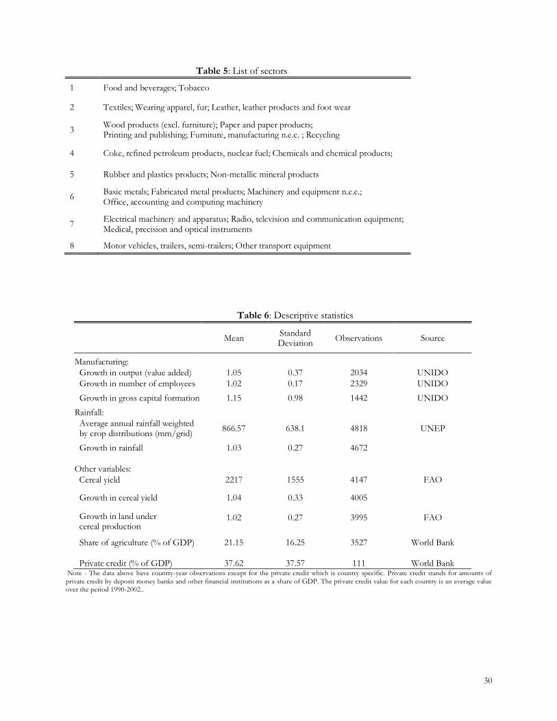
30

Table 5: List of sectors

1 Food and beverages; Tobacco

2 Textiles; Wearing apparel, fur; Leather, leather products and foot wear

3 Wood products (excl. furniture); Paper and paper products; Printing and publishing; Furniture, manufacturing n.e.c. ; Recycling

4 Coke, refined petroleum products, nuclear fuel; Chemicals and chemical products;

5 Rubber and plastics products; Non-metallic mineral products

6 Basic metals; Fabricated metal products; Machinery and equipment n.e.c.; Office, accounting and computing machinery

7 Electrical machinery and apparatus; Radio, television and communication equipment; Medical, precision and optical instruments

8 Motor vehicles, trailers, semi-trailers; Other transport equipment

Table 6: Descriptive statistics

Mean

Standard Deviation

Observations Source

Manufacturing: Growth in output (value added) 1.05 0.37 2034 UNIDO

Growth in number of employees 1.02 0.17 2329 UNIDO

Growth in gross capital formation 1.15 0.98 1442 UNIDO

Rainfall: Average annual rainfall weighted

by crop distributions (mm/grid) 866.57 638.1 4818 UNEP

Growth in rainfall 1.03 0.27 4672

Other variables: Cereal yield 2217 1555 4147 FAO

Growth in cereal yield 1.04 0.33 4005

Growth in land under cereal production

1.02 0.27 3995 FAO

Share of agriculture (% of GDP) 21.15 16.25 3527 World Bank

Private credit (% of GDP) 37.62 37.57 111 World Bank Note - The data above have country-year observations except for the private credit which is country specific. Private credit stands for amounts of

private credit by deposit money banks and other financial institutions as a share of GDP. The private credit value for each country is an average value over the period 1990-2002..

31

Table 7: Crop yield and rainfall (First-stage results)

Dependent variable: Log growth in crop yield,t

PGDP < $4,000 PGDP < $10,000 $10,000 <PGDP <

$20,000 (1) (2) (3) (4) (5) (6) (7)

Log rainfall growth, t

.33*** [11.06]

.33*** [10.85]

.36*** [9.39]

.28*** [12.07]

.28*** [11.88]

.29*** [9.68]

.10*** [3.74]

Tropical region

Log rainfall growth,t

-.28*** [-3.84]

-.28*** [-3.79]

-.31*** [-4.61]

-.23*** [-4.63]

-.23*** [-4.54]

-.26*** [-5.58]

Excess rain,t

Log rainfall growth,t

-.02

[-.34] .01

[.15]

Log rainfall growth, t-1

-.01 [-.25]

-.01 [-.20]

-.01

[-.31] -.01

[-.25]

.06** [2.94]

Tropical region

Log rainfall growth,t-1

.01 [.15]

.01 [.07]

.32

[.62] .32

[.61]

Country fixed effects

no yes yes no yes yes yes

R-square 0.09 0.09 0.09

0.07 0.07 0.07

0.04

F-statistics 38.40 36.83 56.10 46.71 45.16 65.24 7.30

Obervations 1706 1706 1706 2451 2451 2530 395

Note - T-statistics are in brackets. Specifications (2), (5), and (7) are used as first-stage estimations, since excess rain interaction term registers insignificantly. *** p < 0.01, ** p < 0.05, * p < 0.1.

32

Table 8: Manufacturing output and crop yield (Second-stage results)

Dependent variable: Log growth in manufacturing output,t

PGDP < $4,000 PGDP < $10,000 $10,000 <PGDP< $20,000

OLS (1)

IV (2)

FE-OLS (3)

FE-IV (4)

IV (5)

FE-IV (6)

FE-IV (7)

Log yield growth,t-1

.09** [2.20]

.38** [2.49]

.07** [1.55]

.31* [1.91]

.33** [2.57]

.28* [1.85]

-.13 [.42]

Log yield growth,t

.09 [1.47]

.14 [.68]

.09 [1.58]

.06 [.35]

.18

[.84] .12

[.64]

.02 [.03]

Observations 755 720 755 720

1246 1246 290

Average PGDP

$1,851 $1,847 $1,851 $1,847 $3,759 $3,759 $15,312

Note - T-statistics are in brackets. For regressions without fixed effects, error terms are clustered at the country level. The aggregate manufacturing output is in value added and excludes those sectors that use agricultural products as intermediate inputs. The last row reports average per capita income levels of the sample. *** p < 0.01, ** p < 0.05, * p < 0.1.

Table 9: Manufacturing output and crop yield (Second-stage results)

Dependent variable: Log growth in manufacturing output,t

PGDP < $10,000

All Private credit

< 30% Private credit < 30%

& Agriculture > 20%

Exports > 30%

FE-IV (1)

IV (2)

FE-IV (3)

IV (4)

FE-IV (5)

FE-IV (6)

Log yield growth,t-1

.31* [1.91]

.46** [2.29]

.43** [2.46]

.48** [2.20]

.47*** [2.62]

.03 [.07]

Log yield growth,t

.06 [.35]

.18 [1.04]

.15 [.84]

.18

[1.26] .19

[1.05] -.14

[-.25]

Observations 720 783 783 547 547 318

Average PGDP $1,847 $3,435 $3,435 $2,370 $2,370 $4,802

Note - T-statistics are in brackets. For regressions without fixed effects, error terms are clustered at the country level. The aggregate manufacturing output is in value added and excludes those sectors that use agricultural products as intermediate inputs. Private credit represents the amount of credit to private sectors by banks and financial institutions as a share of GDP. Agriculture represents agricultural production share out of GDP. Exports represent the amount of exports in manufacturing as a share of total manufacturing output. *** p < 0.01, ** p < 0.05, * p < 0.1.

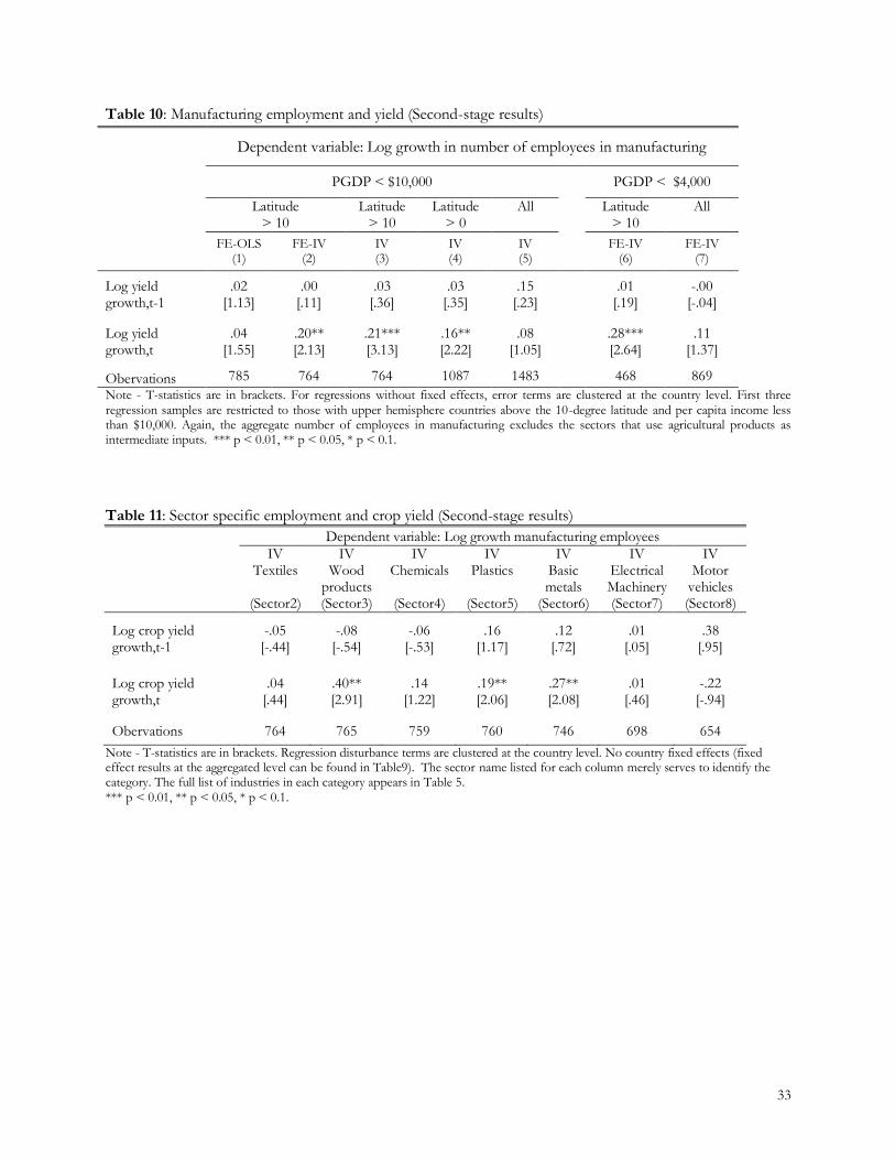
33

Table 10: Manufacturing employment and yield (Second-stage results)

Dependent variable: Log growth in number of employees in manufacturing

PGDP < $10,000 PGDP < $4,000

Latitude > 10

Latitude > 10

Latitude > 0

All

Latitude > 10

All

FE-OLS (1)

FE-IV (2)

IV (3)

IV (4)

IV (5)

FE-IV (6)

FE-IV (7)

Log yield growth,t-1

.02 [1.13]

.00 [.11]

.03 [.36]

.03 [.35]

.15 [.23]

.01 [.19]

-.00 [-.04]

Log yield growth,t

.04 [1.55]

.20** [2.13]

.21*** [3.13]

.16** [2.22]

.08 [1.05]

.28*** [2.64]

.11 [1.37]

Obervations 785 764 764 1087 1483 468 869

Note - T-statistics are in brackets. For regressions without fixed effects, error terms are clustered at the country level. First three regression samples are restricted to those with upper hemisphere countries above the 10-degree latitude and per capita income less than $10,000. Again, the aggregate number of employees in manufacturing excludes the sectors that use agricultural products as intermediate inputs. *** p < 0.01, ** p < 0.05, * p < 0.1.

Table 11: Sector specific employment and crop yield (Second-stage results)

Dependent variable: Log growth manufacturing employees

IV Textiles

(Sector2)

IV Wood

products (Sector3)

IV Chemicals

(Sector4)

IV Plastics

(Sector5)

IV Basic metals

(Sector6)

IV Electrical Machinery (Sector7)

IV Motor

vehicles (Sector8)

Log crop yield growth,t-1

-.05 [-.44]

-.08 [-.54]

-.06 [-.53]

.16 [1.17]

.12 [.72]

.01 [.05]

.38 [.95]

Log crop yield growth,t

.04 [.44]

.40** [2.91]

.14 [1.22]

.19** [2.06]

.27** [2.08]

.01 [.46]

-.22 [-.94]

Obervations 764 765 759 760 746 698 654

Note - T-statistics are in brackets. Regression disturbance terms are clustered at the country level. No country fixed effects (fixed effect results at the aggregated level can be found in Table9). The sector name listed for each column merely serves to identify the category. The full list of industries in each category appears in Table 5. *** p < 0.01, ** p < 0.05, * p < 0.1.

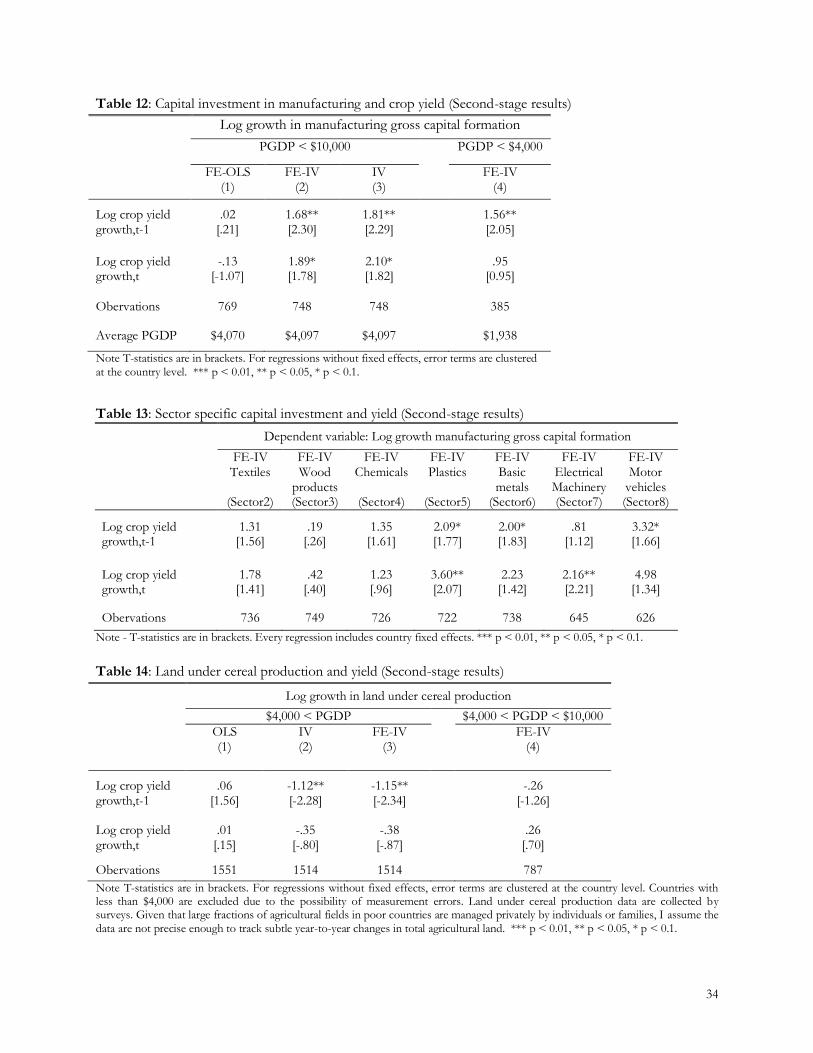
34

Table 12: Capital investment in manufacturing and crop yield (Second-stage results)

Log growth in manufacturing gross capital formation

PGDP < $10,000 PGDP < $4,000

FE-OLS (1)

FE-IV (2)

IV (3)

FE-IV (4)

Log crop yield growth,t-1

.02 [.21]

1.68** [2.30]

1.81** [2.29]

1.56** [2.05]

Log crop yield growth,t

-.13 [-1.07]

1.89* [1.78]

2.10* [1.82]

.95

[0.95]

Obervations 769 748 748 385

Average PGDP $4,070 $4,097 $4,097 $1,938

Note T-statistics are in brackets. For regressions without fixed effects, error terms are clustered at the country level. *** p < 0.01, ** p < 0.05, * p < 0.1.

Table 13: Sector specific capital investment and yield (Second-stage results)

Dependent variable: Log growth manufacturing gross capital formation

FE-IV Textiles

(Sector2)

FE-IV Wood

products (Sector3)

FE-IV Chemicals

(Sector4)

FE-IV Plastics

(Sector5)

FE-IV Basic metals

(Sector6)

FE-IV Electrical Machinery (Sector7)

FE-IV Motor

vehicles (Sector8)

Log crop yield growth,t-1

1.31 [1.56]

.19 [.26]

1.35 [1.61]

2.09* [1.77]

2.00* [1.83]

.81 [1.12]

3.32* [1.66]

Log crop yield growth,t

1.78 [1.41]

.42 [.40]

1.23 [.96]

3.60** [2.07]

2.23 [1.42]

2.16** [2.21]

4.98 [1.34]

Obervations 736 749 726 722 738 645 626

Note - T-statistics are in brackets. Every regression includes country fixed effects. *** p < 0.01, ** p < 0.05, * p < 0.1.

Table 14: Land under cereal production and yield (Second-stage results)

Log growth in land under cereal production

$4,000 < PGDP $4,000 < PGDP < $10,000

OLS (1)

IV (2)

FE-IV (3)

FE-IV (4)

Log crop yield growth,t-1

.06 [1.56]

-1.12** [-2.28]

-1.15** [-2.34]

-.26

[-1.26]

Log crop yield growth,t

.01 [.15]

-.35 [-.80]

-.38 [-.87]

.26

[.70]

Obervations 1551 1514 1514 787

Note T-statistics are in brackets. For regressions without fixed effects, error terms are clustered at the country level. Countries with less than $4,000 are excluded due to the possibility of measurement errors. Land under cereal production data are collected by surveys. Given that large fractions of agricultural fields in poor countries are managed privately by individuals or families, I assume the data are not precise enough to track subtle year-to-year changes in total agricultural land. *** p < 0.01, ** p < 0.05, * p < 0.1.

35

Table 15: Standard deviations of the predicted manufacturing output growth rates

based on the 2SLS-IV results

Countries Volatility of predicted manufacturing output

(%)

Real manufacturing output volatility

(%)

Predicted/Real

Ethiopia 4.13 17.82 0.23

Ghana 4.90 42.98 0.11

Malawi 8.59 16.47 0.52

Uganda 4.53 30.87 0.15

India 2.05 10.91 0.19

Bangladesh 1.98 24.91 0.08

Morocco 17.61 19.69 0.89

44 developing countries (Average values)

5.91 29.25 0.28

Note – The values in column 1 are standard deviations of predicted manufacturing output growth based on the above 2SLS-IV estimation results. Column 2 reports the real manufacturing output volatility directly calculated from the UNIDO (2011) manufacturing output data. “Predicted/real” represents values in column 1 divided

References

Anderson, Kym, and Signe Nelgen. "Trade barrier volatility and agricultural price stabilization." World

Development 40, no. 1 (2012): 36-48.

Anderson, Kym, Maros Ivanic, and Will Martin. "Food Price Spikes, Price Insulation and Poverty." In

The Economics of Food Price Volatility. University of Chicago Press, 2012.

Bastos, Paulo, Odd Rune Straume, and Jaime A. Urrego. "Rain, agriculture, and tariffs." Journal of

International Economics (2013).

Bhalotra, Sonia. "Fatal fluctuations? Cyclicality in infant mortality in India." Journal of Development

Economics 93.1 (2010): 7-19.

Challinor, Andrew, Tim Wheeler, Chris Garforth, Peter Craufurd, and Amir Kassam. "Assessing the

vulnerability of food crop systems in Africa to climate change." Climatic change 83,no. 3 (2007): 81-399.

Chen, Mei-Lien, Chiu-Jung Chen, Wen-Yu Yeh, Ju-Wei Huang, and I-Fang Mao. "Heat stress evaluation

and worker fatigue in a steel plant." AIHA Journal 64, no. 3 (2003): 352-359.

Cline, William R. "Global warming and agriculture: Impact estimates by country." (2008).

36

Dell, Melissa, Benjamin F. Jones, and Benjamin A. Olken. "Temperature shocks and economic growth:

Evidence from the last half century."American Economic Journal:Macroeconomics 4, no. 3(2012): 66-95.

Dercon, Stefan. "Growth and shocks: evidence from rural Ethiopia." Journal of Development Economics

74, no. 2 (2004): 309-329.

Giovanni, Julian di, and Andrei A. Levchenko. "Trade openness and volatility." The Review of Economics

and Statistics 91, no. 3 (2009): 558-585.

Gollin, Douglas, Stephen L. Parente, and Richard Rogerson. "The food problem and the evolution of

international income levels." Journal of Monetary Economics 54, no. 4 (2007): 1230-1255.

Gouel, Christophe. Food price volatility and domestic stabilization policies in developing countries. No.

w18934. National Bureau of Economic Research, 2013.

Haase, Rachel A. Innovation in Emerging Energy Technologies: A case study analysis to inform the path

forward for algal biofuels. Diss. The University of Minnesota, 2012.

Jayachandran, Seema. "Selling labor low: Wage responses to productivity shocks in developing

countries." Journal of Political Economy 114, no. 3 (2006): 538-575.

Jones, Benjamin F., and Benjamin A. Olken. "Climate Shocks and Exports." The American Economic

Review 100, no. 2 (2010): 454-59.

Koren, Miklós, and Silvana Tenreyro. "Technological diversification." The American Economic Review

103, no. 1 (2013): 378-414.

Koren, Miklós, and Silvana Tenreyro. "Volatility and development." The Quarterly Journal of Economics

122, no. 1 (2007): 243-287.

Kose, M. Ayhan. "Explaining business cycles in small open economies:‘How much do world prices

matter?’." Journal of International Economics 56, no. 2 (2002): 299-327.

Kraay, Aart, and Jaume Ventura. "Comparative advantage and the cross‐ section of business cycles."

Journal of the European Economic Association 5, no. 6 (2007): 1300-1333.

Krishna, Pravin, and Andrei A. Levchenko. "Comparative advantage, complexity, and volatility." Journal

of Economic Behavior & Organization (2012).

Lee, Huey-Lin. "The impact of climate change on global food supply and demand, food prices, and land

use." Paddy and water environment 7.4 (2009): 321-331.

Levine, Ross, Norman Loayza, and Thorsten Beck. "Financial intermediation and growth: Causality and

causes." Journal of monetary Economics 46, no. 1 (2000): 31-77.

Lobell, David B., and Christopher B. Field. "Global scale climate–crop yield relationships and the

impacts of recent warming." Environmental Research Letters 2, no. 1 (2007): 014002.

Loening, Josef L., Dick Durevall, and Yohannes A. Birru. "Inflation dynamics and food prices in an

agricultural economy: The case of Ethiopia." (2009).

37

Lucas Jr, Robert E. "On the mechanics of economic development." Journal of monetary economics 22,

no.1 (1988): 3-42.

Martin, Will, and Kym Anderson. "Export restrictions and price insulation during commodity price

booms." American Journal of Agricultural Economics 94, no. 2 (2012): 422-427.

Matsuyama, Kiminori. "Agricultural productivity, comparative advantage, and economic growth."

Journal of economic theory 58, no. 2 (1992): 317-334.

Miguel, Edward, Shanker Satyanath, and Ernest Sergenti. "Economic shocks and civil conflict: An

instrumental variables approach." Journal of political Economy 112, no. 4 (2004): 725-753.

Mundlak, Y., 2001. Production and supply. In: Gardner, B., Rausser, G. (Eds.), Handbook of Agricultural

Economics, vol. 1A. North-Holland, Elsevier, New York, NY, pp. 3–85.

Nicita, Alessandro, and Marcelo Olarreaga. "Trade, production, and protection database, 1976–2004."

The World Bank Economic Review 21, no. 1 (2007): 165-171.

Obstfeld, Maurice. "Models of currency crises with self-fulfilling features." European economic review

40, no. 3 (1996): 1037-1047.

Quiggin, John. "Drought, climate change and food prices in Australia." University of Queensland (2007).

Ramankutty, Navin, Amato T. Evan, Chad Monfreda, and Jonathan A. Foley. "Farming the planet: 1.

Geographic distribution of global agricultural lands in the year 2000." Global Biogeochemical Cycles 22,

no. 1 (2008): GB1003.

Restuccia, Diego, Dennis Tao Yang, and Xiaodong Zhu. "Agriculture and aggregate productivity: A

quantitative cross-country analysis." Journal of Monetary Economics 55, no. 2 (2008): 234-250.

Saint-Paul, Gilles. "Technological choice, financial markets and economic development." European

Economic Review 36, no. 4 (1992): 763-781.

Schlenker, Wolfram, and Michael J. Roberts. "Nonlinear temperature effects indicate severe damages to

US crop yields under climate change." Proceedings of the National Academy of Sciences 106, no. 37

(2009): 15594-15598.

Steger, Thomas. "Economic growth with subsistence consumption." In Transitional Dynamics and

Economic Growth in Developing Countries, pp. 21-60. Springer Berlin Heidelberg, 2000.

Stone, Richard. "Linear expenditure systems and demand analysis: an application to the pattern of British

demand." The Economic Journal 64, no. 255 (1954): 511-527.

Tapia, H., 2012. Volatility and Wealth. mimeo, Columbia University.

United Nations Industrial Development Organization, Industrial Statistics Data-base, 3-digit ISIC, United

Nations Industrial Development Organization,Vienna, 2011.

Van Wijnbergen, Sweder. "The Dutch Disease: a disease after all?." The Economic Journal 94, no. 373

(1984): 41-55.

38

Appendix

A Equilibrium solutions for the closed economy

Appendix A shows the derivation of equilibrium solutions for the benchmark model introduced in section

2 and for the extended model with CES preferences. Recall that a representative agent has a Cobb-

Douglas Stone-Geary utility function:

,

The agent has the following budget constraint:

,

where the manufacturing price is normalized to 1. Solving the utility maximization problem subject to the

budget constraint yields expenditure equations for food and manufacturing as follows:

Also, recall that each industry chooses and to maximize profits,

,

where . The first order conditions are given by,

Using equations A1 and A2, can be expressed in terms of and , and can be expressed in

terms of , yielding

Using the market clearing condition and Eqs. (A1)– (A4), we obtain the following:

Substituting Eq. (A4) for in the above equation, an implicit solution for can be obtained as

follows:

39

where

. All other equilibrium allocations can be obtained from knowing

. 30

CES preferences

Consider a more generalized case with a CES utility function where substitution between expenditures for

food and manufacturing is allowed:

Note that the above utility function converges to the Cobb-Douglas form,

, as . Solving the

above maximization problem yields a manufacturing quantity as follows:

Using the market clearing condition and equations A1 – A4, we obtain the following:

This leads to a non-closed form solution for :

31

where is a function of :

32

CES Stone-Geary preferences

30

31 and

32

.

40

Consider a CES utility function with subsistence consumption on food:

Solving the above maximization problem yields a manufacturing demand as follows:

Using the market clearing condition, and equations A1 – A4, we obtain the following:

33

B Small open economy

In this section, we assume a small open economy where the price is fixed at a world price, .

Note that firms’ profit maximization problems are irrelevant to the demand side since the prices are

already given. Substituting for in Eqs. (A1) and (A2) leads to the following:

Solve for using (A7) and get

.

Combine this with (A4). We can

then derive an equation in terms of only one variable, :

Rearranging the terms, we have a closed form solution for :

34

Notice that the term inside the bracket is increasing with

: if agriculture becomes relatively less

productive than manufacturing, resources shift towards manufacturing. This contrasts with the case of the

closed economy with Stone-Geary preferences in which a negative shock to agricultural productivity,

regardless of the level of manufacturing productivity, pulls resources out of manufacturing and into

agriculture.

33

34

41

Figure A1 plots the relationship between manufacturing output volatility and country’s income

level in open economy. Recall that volatility decreases with income in a closed economy due to the Stone-

Geary effect wearing off. Surprisingly, the figure shows a similar pattern even if consumer’s preference

has nothing to do with output.

Figure A1. Industrial output volatility and development in a small open economy

What drives the negative relationship between volatility and development even in an open

economy? Figure A2 helps answer this question. When resources move between two sectors in response

to shocks, the comparatively disadvantaged sector exhibits higher fluctuation in output growth. This is

because the disadvantaged sector uses a smaller portion of total resources in the economy, so the same

degree of resource reallocation has a larger impact on the disadvantaged sector. In this model, poor

countries have lower amount of capital stock and have a comparative disadvantage in manufacturing,

which leads to the negative relationship between industrial output volatility and income.

Figure A2. Comparative disadvantage and resource movement

42

C Model extensions

This section extends the benchmark model introduced in sections 2 and 3 using a more generalized

version of utility functions, presents simulation results, and compares them with the previous results in

section 3. Moreover, I experiment with the model beyond the assumption of a closed economy in order to

accommodate varying degrees of trade openness to world food markets. By conducting simple alterations

of the original simulation exercises, I examine the differing extent to which agricultural productivity

shocks generate manufacturing output volatility.

C.1 CES preferences

One distinct feature of Cobb-Douglas Stone-Geary preference is that consumers spend a constant fraction

of their residual income on food and manufacturing according to the weights and . In

this section, I relax this condition by replacing Cobb-Douglas Stone-Geary utility functions with CES

Stone-Geary utility functions and study how this changes the results.

Consider a new consumer’s problem with CES Stone-Geary preferences:

35

The above utility function converges to the Cobb-Douglas Stone-Geary utility function,

,

as approaches 1. Solving the above utility maximization problem yields a manufacturing demand

equation as follows:

where

which indicates the fraction of remaining income spent on

manufacturing.

Note that , as . When , has two opposite effects on : (1)

With substitution effects, increases with , as consumers substitute away from food when the

price of food goes up; (2) With income effects, the leftover income decreases with . Since

is inversely related to , the income effect is procyclical with , while the substitution effect is

countercyclical with . In Cobb-Douglas Stone-Geary case, is constant at and there exists only

income effect, while in CES Stone-Geary case both substitution and income effects play roles in

determining equilibrium output in response to shocks to agricultural productivity.

Finally, solving the general equilibrium model with CES Stone-Geary preferences yields the

following implicit solution for (see Appendix A for the derivation):

35 Note that is set at 2.5 for simulations, which means a 1% increase in prices leads to a 2.5% increase in demand.

43

36

where

Simulation results of this new model are presented in Figures A3 and A4 together with the results

from the original model. 37

Note that in the CES Stone-Geary case the degree of the substitution effect is

always constant regardless of the level of income, while the income effect diminishes as a country

becomes richer. Plus, the total effect on manufacturing output caused by an increase in equals the sum

of income effect (positive but decreasing with income level) and substitution effect (negative and

constant). Indeed, manufacturing output elasticity with respect to for CES Stone-Geary is equal to the

elasticity for Cobb-Douglas Stone-Geary plus the substitution effect which is negative. Figure A3 plots

the manufacturing output elasticity against the level of capital stock under the four different assumptions

about preferences: Cobb-Douglas preferences with and without subsistence requirements, and CES

preferences with and without subsistence requirements. Consistent with the analysis, the curve for the

CES Stone-Geary case is placed lower than the one for the Cobb-Douglas Stone-Geary case, and both

elasticities are decreasing with the level of income.

Figure A3. The elasticity of manufacturing output w.r.t. agricultural productivity against per capita capital stock

Figure A4 displays different patterns of manufacturing output volatility against the level of

income across different types of preferences. Note that in the case of CES preferences the volatility is

positive and constant, which is driven solely by the substitution effect – which is counter cyclical - in

36 , , and

37 To generate the figures, I draw an agricultural productivity parameter fifty times independently from a truncated normal

distribution, to construct a series of agricultural productivities,

. For each from 20 to 1000, fifty

corresponding equilibrium manufacturing output values are then calculated for each case. The volatility and elasticity are then calculated based on the equilibrium output values.

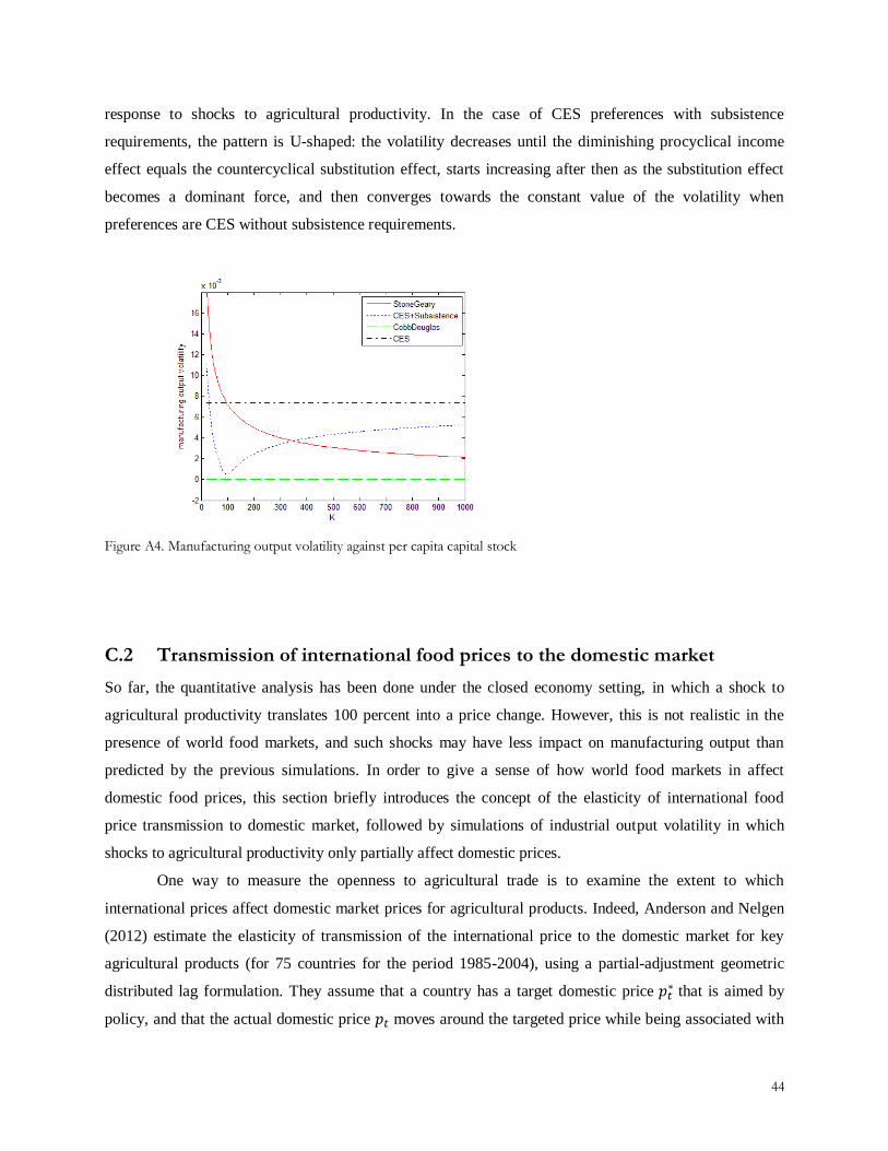
44

response to shocks to agricultural productivity. In the case of CES preferences with subsistence

requirements, the pattern is U-shaped: the volatility decreases until the diminishing procyclical income

effect equals the countercyclical substitution effect, starts increasing after then as the substitution effect

becomes a dominant force, and then converges towards the constant value of the volatility when

preferences are CES without subsistence requirements.

Figure A4. Manufacturing output volatility against per capita capital stock

C.2 Transmission of international food prices to the domestic market

So far, the quantitative analysis has been done under the closed economy setting, in which a shock to

agricultural productivity translates 100 percent into a price change. However, this is not realistic in the

presence of world food markets, and such shocks may have less impact on manufacturing output than

predicted by the previous simulations. In order to give a sense of how world food markets in affect

domestic food prices, this section briefly introduces the concept of the elasticity of international food

price transmission to domestic market, followed by simulations of industrial output volatility in which

shocks to agricultural productivity only partially affect domestic prices.

One way to measure the openness to agricultural trade is to examine the extent to which

international prices affect domestic market prices for agricultural products. Indeed, Anderson and Nelgen

(2012) estimate the elasticity of transmission of the international price to the domestic market for key

agricultural products (for 75 countries for the period 1985-2004), using a partial-adjustment geometric

distributed lag formulation. They assume that a country has a target domestic price that is aimed by

policy, and that the actual domestic price moves around the targeted price while being associated with

45

international price . They suggest a relationship between the target domestic price and the international

market price as follows:

where all prices are expressed in logarithms, and are the domestic and international market prices

in the base period, and is the long-run price transmission elasticity. Anderson and Nelgen (2012)

additionally define the relationship between the target and the actual prices as follows:

where the parameter implies the fraction of the adjustment within 1 year. Substituting (14) into (15)

yields the following estimating equation:

They define the short-run elasticity of price transmission as , which is the regression

coefficient . The long-run elasticity can then be recovered by . The estimated short-run

elasticities for rice, wheat, and maize Anderson and Nelgen (2012) are 0.52, 0.47, and 0.57, respectively.

Similarly, international prices do not fully determine the domestic market prices. This implies that the

domestic supply and demand are partially responsible for fluctuations in domestic agricultural prices.

Meanwhile, the previous regression results are generated under a closed economy, which causes a

change in agricultural productivity to affect the equilibrium food prices 100 percent. However, as can be

seen above, this might not be the case due to the existence of international food market and government

intervention. Thus, taking into account the limiting effect of domestic agriculture supply shock on food

prices, I recalculate manufacturing output volatility while varying the extent to which a change in

agricultural productivity affects food prices and manufacturing output. In order to do that, I introduce a

new agricultural productivity term as follows:

where and stands for domestic agricultural productivity. I subject to shocks while fixing

, which implies that the domestic shocks affect only a fraction of the entire food price. In other

words, can be seen as the degree of openness to the world food market with fixed international

prices. Table A1 reports newly simulated manufacturing output volatilities using with varying based

on the calibrated parameters (I plug crop yield data in in (A8) and obtain that serves as new

agricultural productivity in the original equilibrium model.). The manufacturing output volatility

increases with , which is obvious as impact of the shocks is limited by . Although this approach to

incorporate the partial openness to the world market in the existing model is not quite theoretically

correct, this exercise offers an opportunity to think about alleviating domestic shocks in the presence of a

reliable world food market.

46

Table A1: Varying degrees of transmission of agricultural productivity shocks into equilibrium manufacturing

output with and simulated volatilities

Country

Simulated manufacturing output volatility (%)

a = 0.2 a = 0.4 a = 0.6 a =0.8

Ethiopia 8.06 16.10 24.69 30.83

Ghana 3.21 5.92 9.03 12.33

Malawi 7.54 14.81 22.34 29.19

Uganda 3.39 6.71 9.47 13.05

India 0.46 0.97 1.61 2.48

Bangladesh 0.35 0.72 1.14 1.67

Portugal 0.50 0.97 1.49 2.15

United States 0.12 0.24 0.37 0.51

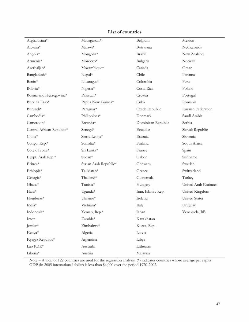
47

List of countries

Afghanistan* Madagascar* Belgium

Mexico

Albania*

Malawi*

Botswana

Netherlands

Angola*

Mongolia*

Brazil

New Zealand

Armenia*

Morocco*

Bulgaria

Norway

Azerbaijan*

Mozambique* Canada

Oman

Bangladesh* Nepal*

Chile

Panama

Benin*

Nicaragua*

Colombia

Peru

Bolivia*

Nigeria*

Costa Rica

Poland

Bosnia and Herzegovina* Pakistan*

Croatia

Portugal

Burkina Faso* Papua New Guinea* Cuba

Romania

Burundi*

Paraguay*

Czech Republic Russian Federation

Cambodia*

Philippines*

Denmark

Saudi Arabia

Cameroon*

Rwanda*

Dominican Republic Serbia

Central African Republic* Senegal*

Ecuador

Slovak Republic

China*

Sierra Leone* Estonia

Slovenia

Congo, Rep.* Somalia*

Finland

South Africa

Cote d'Ivoire* Sri Lanka*

France

Spain

Egypt, Arab Rep.* Sudan*

Gabon

Suriname

Eritrea*

Syrian Arab Republic* Germany

Sweden

Ethiopia*

Tajikistan*

Greece

Switzerland

Georgia*

Thailand*

Guatemala

Turkey

Ghana*

Tunisia*

Hungary

United Arab Emirates

Haiti*

Uganda*

Iran, Islamic Rep. United Kingdom

Honduras*

Ukraine*

Ireland

United States

India*

Vietnam*

Italy

Uruguay

Indonesia*

Yemen, Rep.* Japan

Venezuela, RB

Iraq*

Zambia*

Kazakhstan

Jordan*

Zimbabwe*

Korea, Rep.

Kenya*

Algeria

Latvia

Kyrgyz Republic* Argentina

Libya

Lao PDR*

Australia

Lithuania

Liberia*

Austria

Malaysia

Note – A total of 122 countries are used for the regression analysis. (*) indicates countries whose average per capita GDP (in 2005 international dollar) is less than $4,000 over the period 1970-2002.