
Indoor Location-based Recommender System · 1.2 Thesis Organization ... marketing tool that have...
74
Indoor Location-based Recommender System by Zhongduo Lin A thesis submitted in conformity with the requirements for the degree of Master of Applied Science Graduate Department of Electrical and Computer Engineering University of Toronto Copyright c 2013 by Zhongduo Lin
Transcript of Indoor Location-based Recommender System · 1.2 Thesis Organization ... marketing tool that have...

Indoor Location-based Recommender System
by
Zhongduo Lin
A thesis submitted in conformity with the requirementsfor the degree of Master of Applied Science
Graduate Department of Electrical and Computer EngineeringUniversity of Toronto
Copyright c© 2013 by Zhongduo Lin

Abstract
Indoor Location-based Recommender System
Zhongduo Lin
Master of Applied Science
Graduate Department of Electrical and Computer Engineering
University of Toronto
2013
WiFi-based indoor localization is emerging as a new positioning technology. In this
work, we present our efforts to find the best recommender system based on the indoor
location tracks collected from the Bow Valley shopping mall for one week. The time a user
spends in a shop is considered as an implicit preference and different mapping algorithms
are proposed to map the time to a more realistic rating value. A new distribution error
metric is proposed to examine the mapping algorithms. Eleven different recommender
systems are built and evaluated in terms of accuracy and execution time. The Slope-One
recommender system with a logarithmic mapping algorithm is finally selected with a
score of 1.292, distribution error of 0.178 and execution time of 0.39 seconds for ten runs.
ii

Acknowledgements
I would like to thank my supervisor, Prof. Paul Chow, for his great guidance throughout
the past two years. Thank you for allowing me to explore what I like and giving me full
support when I didn’t do well in my work.
I also want to acknowledge all the support from my group members, who are always
willing to help me whenever needed.
Thank all my colleagues in CISCO Systems, especially my mentor Vince Mammoliti.
Thank you for being such a great friend and philosopher.
I greatly appreciate the encouragement from all my friends in the past two years.
Thank you for cheering me up when I am down.
iii

Contents
1 Introduction 1
1.1 Contribution . . . . . . . . . . . . . . . . . . . . . . . . . . . . . . . . . . 3
1.2 Thesis Organization . . . . . . . . . . . . . . . . . . . . . . . . . . . . . . 3
2 Recommender System Overview 5
2.1 Recommender System Model . . . . . . . . . . . . . . . . . . . . . . . . . 5
2.2 Recommender System Classifications . . . . . . . . . . . . . . . . . . . . 7
2.2.1 Categories based on solutions . . . . . . . . . . . . . . . . . . . . 7
2.2.2 Categories based on information collecting methods . . . . . . . . 9
2.2.3 Categories based on evaluation methods . . . . . . . . . . . . . . 11
2.3 Collaborative Filtering Algorithms . . . . . . . . . . . . . . . . . . . . . 13
2.3.1 User-based CF algorithm . . . . . . . . . . . . . . . . . . . . . . . 14
2.3.2 Item-based CF algorithm . . . . . . . . . . . . . . . . . . . . . . . 15
2.3.3 Slope-One algorithm . . . . . . . . . . . . . . . . . . . . . . . . . 16
2.3.4 Similarity metrics . . . . . . . . . . . . . . . . . . . . . . . . . . . 18
3 Related Work 20
4 Collecting Data 25
4.1 Indoor Localization with WiFi . . . . . . . . . . . . . . . . . . . . . . . . 25
4.2 Data Collection Architecture . . . . . . . . . . . . . . . . . . . . . . . . . 27
iv

4.3 The Bow Valley Square Data Set . . . . . . . . . . . . . . . . . . . . . . 29
4.3.1 Definition of terms . . . . . . . . . . . . . . . . . . . . . . . . . . 29
4.3.2 Building test beds . . . . . . . . . . . . . . . . . . . . . . . . . . . 30
4.3.3 Accuracy analysis . . . . . . . . . . . . . . . . . . . . . . . . . . . 33
4.3.4 Preprocessing algorithms . . . . . . . . . . . . . . . . . . . . . . . 34
4.3.5 Statistical analysis . . . . . . . . . . . . . . . . . . . . . . . . . . 34
5 Building the Recommender Systems 38
5.1 System Overview . . . . . . . . . . . . . . . . . . . . . . . . . . . . . . . 38
5.1.1 Interaction between MSE and device . . . . . . . . . . . . . . . . 40
5.1.2 Interaction between MSE and server . . . . . . . . . . . . . . . . 40
5.1.3 Interaction between server and device . . . . . . . . . . . . . . . . 41
5.2 Mahout . . . . . . . . . . . . . . . . . . . . . . . . . . . . . . . . . . . . 42
5.3 Implicit Preference Mapping Functions . . . . . . . . . . . . . . . . . . . 44
5.3.1 Mapping functions . . . . . . . . . . . . . . . . . . . . . . . . . . 45
5.3.2 Evaluation metrics . . . . . . . . . . . . . . . . . . . . . . . . . . 48
6 Methodology and Evaluation 51
6.1 Methodology . . . . . . . . . . . . . . . . . . . . . . . . . . . . . . . . . 51
6.1.1 Experimental platform . . . . . . . . . . . . . . . . . . . . . . . . 51
6.1.2 Test cases . . . . . . . . . . . . . . . . . . . . . . . . . . . . . . . 52
6.1.3 Evaluation methods . . . . . . . . . . . . . . . . . . . . . . . . . . 52
6.2 Evaluation . . . . . . . . . . . . . . . . . . . . . . . . . . . . . . . . . . . 53
6.2.1 Evaluation of non-scaling mapping functions . . . . . . . . . . . 53
6.2.2 Evaluation of mapping functions with scaling . . . . . . . . . . . 55
6.2.3 Execution time evaluation . . . . . . . . . . . . . . . . . . . . . . 57
7 Conclusion 59
v

8 Future Work 60
Bibliography 62
vi

List of Tables
2.1 Term definitions for different RSs . . . . . . . . . . . . . . . . . . . . . . 6
2.2 A simple example of a utility matrix . . . . . . . . . . . . . . . . . . . . 6
2.3 Classification of recommender systems research [1] . . . . . . . . . . . . . 10
2.4 A simple example of average difference and root-mean-square difference. [2] 12
5.1 GroupLens 1M breakdown . . . . . . . . . . . . . . . . . . . . . . . . . . 50
6.1 Comparison of RSs with non-scaling mapping functions . . . . . . . . . . 54
6.2 Comparison of RSs with scaling mapping functions . . . . . . . . . . . . 56
6.3 Distribution error for scaling mapping functions . . . . . . . . . . . . . . 56
6.4 Comparison in terms of execution time . . . . . . . . . . . . . . . . . . . 58
vii

List of Figures
4.1 Typical wireless controller to AP deployment for location [3] . . . . . . . 27
4.2 MSE High Level Architecture [3] . . . . . . . . . . . . . . . . . . . . . . 28
4.3 Interaction with the MSE API [3] . . . . . . . . . . . . . . . . . . . . . . 32
4.4 Device occurrence distribution . . . . . . . . . . . . . . . . . . . . . . . . 35
4.5 Number of points per path . . . . . . . . . . . . . . . . . . . . . . . . . . 36
4.6 Path duration distribution . . . . . . . . . . . . . . . . . . . . . . . . . . 37
5.1 Service System Overview . . . . . . . . . . . . . . . . . . . . . . . . . . . 39
5.2 Mahout Framework . . . . . . . . . . . . . . . . . . . . . . . . . . . . . . 43
5.3 Implicit recommender system overview . . . . . . . . . . . . . . . . . . . 46
6.1 User-based RS with non-scaling mapping functions . . . . . . . . . . . . 54
6.2 User-based RS with scaling mapping functions . . . . . . . . . . . . . . . 55
viii

Chapter 1
Introduction
In the 2002 movie, Minority Report [4], Tom Cruise walks through a shopping mall and is
targeted with personalized advertising. This is a highly sophisticated form of a Location-
Based Service that provides a service based on the location of a user. The advertising
Cruise receives also recommends products, such as cars and beer. This is a Recommender
System (RS) that utilizes the location-based service to make a recommendation based on
the user’s location. This thesis develops the first WiFi-based Recommender System as a
platform for further exploration of such systems.
With the development of sensing and automated means of perceiving the physical
environment, it is possible to collect much more implicit context with our everyday
electronic devices such as smart phones, or personal digital assistants (PDA). Among
these contexts, Ljungstrand [5] predicted that location-based services (LBSs) [6] will be
the most common form of context-aware computing [7].
Traditionally, LBSs were designed to support outdoor applications such as navigation
and fleet management. While the Global Positioning System (GPS) [8] has achieved a
great success and popularity all over the world in the recent decade, indoor LBSs are a
marketing tool that have the potential to increase business profit. The growing interest in
this technology can be demonstrated by the recent actions of large technology companies.
1

Chapter 1. Introduction 2
1. March 24th, 2013, Apple acquired WiFiSlam [9], an indoor GPS startup that en-
ables a smart phone to pinpoint its location.
2. September 26th, 2012, Cisco announced the acquisition of ThinkSmart Technolo-
gies [10], a startup that analyses indoor location information based on Cisco’s
wireless networking infrastructure.
3. April 27th, 2010, Google [11] submitted a white paper to several national data
protection authorities on vehicle-based collection of WiFi data for use in Google
location-based services.
Often used in conjunction with a LBS is a Recommender System (RS). Recommender
systems [12, 13, 14] are a subclass of information filtering systems that seek to predict the
rating or preference that a user would give to an item (such as music, books, or movies)
or social element (e.g. people or groups) they had not yet considered, using a model
built from the characteristics of an item (content-based approaches) or the user’s social
environment (collaborative filtering approaches). It has become an extremely common
context aware service in recent years. One main area of research has been focused on
building recommender systems based on user trajectories. Application domains include
mobile social networking, tourism guides, urban computing and information retrieval.
While there are a few research papers published recently about location-based recom-
mender systems using GPS tracks, there are even fewer for indoor LBSs due to the lack
of a standard for indoor positioning, which will be discussed in Chapter 4. Compared
to GPS, WiFi-based indoor positioning systems introduce different noise due to the in-
stability of WiFi signals, and present unique characteristics that will be discussed in
Section 4.1.

Chapter 1. Introduction 3
1.1 Contribution
This work details our efforts to find the best recommender system implementation based
on the real-world mobile tracks in a shopping mall, aiming to recommend the shops in the
mall that will interest the customers according to their track history. Over ten thousand
customers are tracked for a week in the Bow Valley Square shopping mall [15]. This data
is used to develop a recommender system to predict the preferences a user will give to
all the shops based on the data set and recommend the top shops to the user.
The main contributions of this work are:
1. The first time building of a location-based recommender system using WiFi posi-
tioning technology;
2. A comparison between different recommender systems using WiFi positioning;
3. The proposal of different mapping functions for implicit information and a new
evaluation metric for the mapping functions
Though this work only focuses on a specific data set, it is expected that the methods
developed in this thesis will work on other applications using the same positioning infras-
tructure. For example, CISCO’s acquisition, ThinkSmart Technology, has demonstrated
success on other applications such as airport planning and museum tour guide systems
using the same positioning system.
1.2 Thesis Organization
The remainder of this thesis is organized as follows. Chapter 2 provides an overview of the
state-of-the-art technologies used in recommender systems and the different categories
of recommender systems. This overview will help with understanding the basic data
collection methods in Chapter 4 and evaluation methodology in Chapter 6. A list of

Chapter 1. Introduction 4
related work, including outdoor location-based recommender systems and generic services
based on indoor location, is presented in Chapter 3. Chapter 4 details our data collecting
method and a simple analysis of the data set. Chapter 5 presents the whole process of
building the recommender systems. Our methodology and evaluation results are detailed
in Chapter 6. Chapter 7 provides the conclusion and Chapter 8 describes future work.

Chapter 2
Recommender System Overview
The interest in recommender systems has been high among industry and academia since
the mid-1990s when the first papers on collaborative filtering were published and proved
to be useful [16, 17, 18]. Then there was a significant boost to research into recommender
systems when NetFlix offered a prize of $1,000,000 to the first person or team to beat
their own recommender algorithm, CineMatch, by 10% [2]. This chapter will briefly
introduce the basic ideas, concepts and techniques for general recommender systems. A
more detailed and comprehensive overview on recommender systems can be found in [19].
2.1 Recommender System Model
There are three subjects in the data sets used to build a recommender system: user,
item and preference. Since the Amazon book recommender system [20] is more familiar
to the audience, it is taken as an analogy to help illustrate these three terms along with
the shop recommender system (Shop RS) developed in this thesis, .
Table 2.1 shows a comparison between the Amazon Book RS and Shop RS in terms
of the definitions of the three subjects. Generally, the users refer to the customers who
make the decisions and are the ones that the recommender systems aim to recommend
items to. The items refer to different objects available for the users to choose. They can
5

Chapter 2. Recommender System Overview 6
Table 2.1: Term definitions for different RSs
Amazon Book RS Shop RS
user customers on the online system customers in the shopping mall
item books on the system shops in the shopping mall
preference ratings given by users to items time users spend in certain shops
Table 2.2: A simple example of a utility matrix
User ID CIBC Copy Centre Rise Bakery Cafe X-Press Second Cup
6 315 931
56 340 1023 80
135 80 648 2156
be books for the Amazon Book RS, places for a tourism recommender system, etc. The
preference refers to the degree that a user likes a certain item. The most popular way
to represent the preference is by the explicit rating values ranging from 1 to 5, which is
used by the Amazon online system [20] and BestBuy [21]. They can also be implied by
user behaviours like clicks or time spent in a certain web page, which will be discussed
later in Section 2.2.
The data set used in a recommender system is always represented by a matrix that is
referred to as a utility matrix. A simple example for Shop RS is illustrated in Table 2.2.
The users are represented by their user IDs such as 56 in the leftmost column, while the
items are represented by the names of the shops. The preference values in the example
are the actual number of seconds the user spent in the shops. Notice that most values
in the preference field are left blank, which indicates that the users have never entered
the corresponding shops. In reality, since a row in the utility matrix will include all the
preferences to each shop in the shopping mall, the matrix will be much more sparse than
that in the example, with the typical user only visiting a tiny fraction of all the available
shops.

Chapter 2. Recommender System Overview 7
2.2 Recommender System Classifications
There are many different ways to classify and identify a recommender system based
on certain attributes or techniques used. Similar to [13], in this section we focus on
the three major attributes that apply to most recommender systems, and can be used to
identify the recommender system developed in this thesis – the recommendation solutions
adopted, the information collection methods and the evaluation methods.
2.2.1 Categories based on solutions
A blank preference can be estimated in different ways using methods from machine
learning, approximation theory and various heuristics. A recommender system solution
refers to the way the recommender system is built. Following the classifications in [22],
the recommender systems can be classified into three categories based on their approach:
1. Content-based recommender: The RS recommends items similar to the ones the
user preferred in the past,
2. Collaborative recommender: The RS recommends items that similar users preferred
in the past,
3. Hybrid recommender: A combined approach using both content-based recom-
mender and collaborative recommender.
In a content-based recommender, a record or collection of records representing im-
portant characteristics of an item, which is often referred to as an item profile, must
be constructed to classify different items. For example, in a music recommender sys-
tem, a profile can include features such as the composer, the singer, the genre and the
year. There are various techniques to automatically extract characteristics from items,
among which the most widely used one is Term Frequency/Inverse Document Frequency
(TF-IDF) that is used to specify keyword weights in text-based items. The idea of

Chapter 2. Recommender System Overview 8
content-based recommender systems is based on the fact that people tend to like items
that are similar to their preference. Assuming that some users like a song from Avril
Lavigne, it is likely that they will like other songs from her. While this approach works
quite well in practice, it suffers from several drawbacks:
1. Limited content analysis: Not only is it time consuming when some features, such
as music genre, have to be entered manually, but it is not sufficient to reflect the
different quality or popularity among items with the same features.
2. Domain-specialization: It is almost impossible to decide a set of general features
for all the items. For example, a book can be well described by its page count,
author and publisher, while none of these features can be applied to a bookmark.
However, one can easily see the connection between a book and a bookmark.
These drawbacks prevent researchers from developing a general framework for content-
based recommender systems [2]. An alternative way is to use collaborative methods,
which is enjoying a high interest among researchers and is also the approach of this
thesis. Instead of depending on the features of items to determine their similarity, it
leverages the similarity of the user ratings for co-rated items. More details about the
collaborative approach will be discussed in Section 2.3. The main limitation of this
approach is the sparsity of the user ratings. In any recommender system, the number of
ratings already obtained is usually very small compared to the number of ratings that
have to be predicted. For example, there may be millions of books in the Amazon book
recommender system, while the average number of books that a user rates may be below
five.
To overcome the limitations of content-based and collaborative recommender sys-
tems, a hybrid approach is proposed by combining collaborative and content-based rec-
ommender techniques. Almost all modern recommender systems can be classified into
this category since they more or less utilize techniques from both content-based and col-

Chapter 2. Recommender System Overview 9
laborative methods. Depending on the different ways to combine these two methods, the
hybrid recommender systems can be further classified as: (1) combining totally separate
recommender systems, (2) adding the characteristics of one to the other, (3) construct-
ing a general unifying model that incorporates the characteristics of both recommender
systems. Since this is not the focus of this thesis, the discussion will end here. More
details can be found in [1].
Table 2.3, reproduced from [1], shows a comprehensive summary of techniques used
in each category and example research efforts. A brief introduction to heuristic-based
and model-based techniques is described in Section 2.3.
2.2.2 Categories based on information collecting methods
Information collecting methods refer to the ways that user feedback is collected. Depend-
ing on the level of user involvement, recommender systems can be classified as follows:
1. Intrusive recommender system: A significant level of user involvement is required
to get the feedback.
2. Non-intrusive recommender system: Little or no explicit user involvement is re-
quired to get the feedback.
Most of the practical recommender systems now fall into the intrusive recommender
systems. The most widely used way to collect user feedback is to explicitly ask users
to rate the items they have reviewed or purchased. For example, in almost all the
online shopping systems such as BestBuy and eBay, customers are encouraged to rate
the items they bought. While being predominant, intrusive recommender systems suffer
from the fact that users are lazy in that they would not bother to even come up with the
appropriate rating [17], resulting in an extremely small number of ratings per user.
An alternative way to get feedback is to leverage certain proxies to estimate the real
rating a user will give to an item. Minimizing intrusiveness while keeping the accuracy

Chapter 2. Recommender System Overview 10
Table 2.3: Classification of recommender systems research [1]
25
Recommendation Technique Recommendation Approach Heuristic-based Model-based
Content-based Commonly used techniques: • TF-IDF (information retrieval) • Clustering
Representative research examples: • Lang 1995 • Balabanovic & Shoham 1997 • Pazzani & Billsus 1997
Commonly used techniques: • Bayesian classifiers • Clustering • Decision trees • Artificial neural networks
Representative research examples: • Pazzani & Billsus 1997 • Mooney et al. 1998 • Mooney & Roy 1999 • Billsus & Pazzani 1999, 2000 • Zhang et al. 2002
Collaborative Commonly used techniques: • Nearest neighbor (cosine, correlation) • Clustering • Graph theory
Representative research examples: • Resnick et al. 1994 • Hill et al. 1995 • Shardanand & Maes 1995 • Breese et al. 1998 • Nakamura & Abe 1998 • Aggarwal et al. 1999 • Delgado & Ishii 1999 • Pennock & Horwitz 1999 • Sarwar et al. 2001
Commonly used techniques: • Bayesian networks • Clustering • Artificial neural networks • Linear regression • Probablistic models
Representative research examples: • Billsus & Pazzani 1998 • Breese et al. 1998 • Ungar & Foster 1998 • Chien & George 1999 • Getoor & Sahami 1999 • Pennock & Horwitz 1999 • Goldberg et al. 2001 • Kumar et al. 2001 • Pavlov & Pennock 2002 • Shani et al. 2002 • Yu et al. 2002, 2004 • Hofmann 2003, 2004 • Marlin 2003 • Si & Jin 2003
Hybrid Combining content-based and collaborative components using:
• Linear combination of predicted ratings • Various voting schemes • Incorporating one component as a part of
the heuristic for the other Representative research examples:
• Balabanovic & Shoham 1997 • Claypool et al. 1999 • Good et al. 1999 • Pazzani 1999 • Billsus & Pazzani 2000 • Tran & Cohen 2000 • Melville et al. 2002
Combining content-based and collaborative components by:
• Incorporating one component as a part of the model for the other
• Building one unifying model Representative research examples:
• Basu et al. 1998 • Condliff et al. 1999 • Soboroff & Nicholas 1999 • Ansari et al. 2000 • Popescul et al. 2001 • Schein et al. 2002
Table 2: Classification of recommender systems research.
3.1. Comprehensive understanding of users and items
As was pointed out in [2, 8, 54, 105], most of the recommendation methods produce ratings that
are based on a limited understanding of users and items as captured by user and item profiles and
do not take full advantage of the information in the user's transactional histories and other
Chapter 2. Recommender System Overview 11
of recommendations is still an important research topic because of its difficulty and
promising potential. The non-intrusive approach is mostly used in online systems such
as newsgroup article recommender systems and the most common proxies are the click
behaviour and the time spent on a article. Morita and Shinoda [23] have found that user
preference to NetNews articles are well reflected by the time spent reading these articles
regardless of the length of the article.
The recommender system described in this thesis is one of the non-intrusive recom-
mender systems, since the time users spend in a certain shop is used as a proxy to estimate
their ratings. After determining the proxy, another important factor that will influence
the efficiency of the recommender system is how to actually derive the appropriate es-
timation of preference from the implicit information. Different mapping functions are
discussed in Chapter 5.
2.2.3 Categories based on evaluation methods
A recommender system is a tool to generate the best recommendations. Therefore, before
making a recommendation to the user, the recommender system should determine which
recommendation is the best one. The ideal recommender would be a psychic that could
know exactly user preferences towards different items. However, unlike cases such as
solving a mathematical problem, where a golden key exists and can be used to examine
an algorithm, no one can know exactly how much a user will like a new item, including
the user itself, in a recommender system. Different recommender systems are trying to
achieve a certain goal that they believe will result in the best recommendation. This
goal, though it will never be perfect, is referred to as the evaluation method. The two
most prevailing evaluation methods are:
1. Scoring: Set aside a small part of the real data set as test data set, then estimate
the test set with the remaining data set, and finally compare the difference between
the estimated values and the real ones.

Chapter 2. Recommender System Overview 12
Table 2.4: A simple example of average difference and root-mean-square difference. [2]
Item 1 Item 2 Item 3
actual value 3.0 5.0 4.0
estimated value 3.5 2.0 5.0
difference 0.5 3.0 1.0
average difference =(0.5+3.0+1.0)/3=1.5
root-mean-square =√
(0.52 + 3.02 + 1.02)/3 = 1.8
2. Precision and recall: Similar to the scoring method, but instead of comparing val-
ues, the top n items are returned for each user. The items are then used to calculate
the precision and recall. Precision is the proportion of top recommendations that
are good recommendations (existing highly rated items) and recall is the proportion
of good recommendations that appear in top recommendations.
The precision and recall method is not used in this thesis because it generally requires
a relatively large number of ratings from the users, which is not applicable to this work.
A more detailed description can be found in [2]. For the scoring evaluation method,
after getting the estimated preference values from a collaborative filtering algorithm, the
recommender systems need to determine the overall error metric they want to minimize.
Average difference and root-mean-square of the differences are the two most common
metrics to use. Table 2.4 gives a simple example to illustrate how these two error metrics
work. The two metrics are similar in terms of the quality of recommendations. The
average difference is adopted in this thesis. A smaller value indicates better performance
of the recommender system.

Chapter 2. Recommender System Overview 13
2.3 Collaborative Filtering Algorithms
A collaborative recommender system tries to estimate the unknown ratings based on
the items previously rated by other users. Therefore, unlike a content-based approach,
a collaborative recommender system can only depend on the ratings rather than any
domain specific information of items. According to Breese [24], collaborative filtering
algorithms can be classified into two groups:
1. Heuristic-based: Make rating estimations based on the entire collection of previ-
ously rated items by the users.
2. Model-based: Use the collection of ratings to learn a model that will be used to
make rating predictions.
The model-based collaborative filtering algorithms are getting more and more atten-
tion recently as the interest in machine learning grows among academia. Many techniques
such as artificial neural networks, singular value decomposition and clustering are lever-
aged to learn different models for recommender systems and are proven to be efficient in
many applications [1]. Despite its great potential, it is not implemented in this thesis.
Instead, the simplest-first approach is taken because the goal is to first implement a com-
plete system that can then be studied and measured to determine where improvements
are required.
The heuristic-based collaborative filtering (CF) algorithms are the focus of this thesis.
They are widely used because of their simplicity and efficiency. They can be further
divided into two categories:
1. User-based CF algorithm: Estimate the unknown ratings based on other similar
users.
2. Item-based CF algorithm: Estimate the unknown ratings based on the similarities
between the target item and other items that are co-rated by the the same user.

Chapter 2. Recommender System Overview 14
2.3.1 User-based CF algorithm
The shopping mall case in this thesis is taken as an example to illustrate how the user-
based CF algorithm works. Around Christmas, there will be many people going to the
shopping mall to prepare for a Christmas party. Most of them will go to the candy shop,
the gift shop and the decoration shop during their visits. So if a customer has already
been to the candy shop and the gift shop, then it can be inferred that he or she is similar
to those who are preparing for a Christmas party and the decoration shop can be a good
recommendation to the customer.
The reasoning is intuitive because people tend to like things that similar customers
like. The first problem is how to define the similarity metrics, which will be discussed in
Section 2.3.4. Several terms, which will be used in this section, need to be defined before
the algorithm is introduced.
1. Similarity: How similar a user is to another one in terms of their ratings to the
items that both rated.
2. Nearest neighbours: The users that are most similar to a certain user according to
the similarity metric.
3. Neighbourhood size: The number of the neighbours used in a user-based recom-
mender system.
Algorithm 1 lists a generic user-based algorithm. The first for loop aims to get
the n nearest neighbours of each user. Note that we can simply ignore this step to
include all the other users in the second for loop, which is equivalent to setting n to
infinity. However, setting an appropriate value to n will accelerate the computation and
always result in better recommendations, because more similar users tend to provide more
reliable predictions. The second for loop estimates the unknown ratings by calculating
a weighted average of ratings that the n nearest neighbours give to the items.

Chapter 2. Recommender System Overview 15
for every other user w do
compute a similarity s between u and w;
retain the top users, ranked by similarity, as a neighbourhood n;
end
for every item i that some user in n has a preference for, but u has no preference
for yet do
for every other user v in n that has a preference for i do
compute a similarity s between u and v;
incorporate v’s preference for i, weighted by s, into a running average;
end
end
Algorithm 1: User-based collaborative filtering algorithm [2]
2.3.2 Item-based CF algorithm
The same example in Section 2.3.1 is taken to illustrate how the item-based CF algorithm
works. Around Christmas, there will be many people going to the candy shop, the gift
shop and the decoration shop. So if a customer has already been to the candy shop
and the gift shop, then it can be concluded that since the candy shop, the gift shop and
the decoration shop tend to be visited altogether, the decoration shop can be a good
candidate to recommend to the customer.
Though the recommendation result of this item-based approach is the same as the
user-based one, the basis to draw the conclusion is different. The recommendation is
based on the similarity of shops regardless of the users. Therefore, the term nearest
neighbours does not exist in the item-based CF algorithms. The similarity, however, still
needs to be calculated though from a different perspective.
Algorithm 2 lists a generic item-based algorithm. The outer for loop iterates all the
items that a user has not rated yet. The inner for loop calculates the weighted average

Chapter 2. Recommender System Overview 16
for every item i that u has no preference for yet do
for every item j that u has a preference for do
compute a similarity s between i and j;
add u’s preference for j, weighted by s, to a running average;
end
end
return the top items, ranked by weighted average;
Algorithm 2: Item-based collaborative filtering algorithm [2]
of the ratings of items that the user has already rated. Note that the similarity s here
refers to the similarity between items instead of users.
There are several advantages of the item-based approach compared to the user-based
one:
1. Scalability: The run time of an item-based recommender system scales up as the
number of items increases, thus if the number of items is relatively low compared
to the number of users, an item-based recommender system is more preferable.
2. Less subject to change: Over time the similarities between items tend to converge,
while user tastes can vary vastly. Therefore, an item-based recommender system
typically can start making reasonable recommendations after a user’s first rating,
while user-based ones need enough ratings to find nearest neighbours.
3. Able to be preprocessed: Since the item-item similarities are more fixed, it is rea-
sonable to precompute them to speed up the execution time.
2.3.3 Slope-One algorithm
The Slope-One item-based collaborative algorithm was proposed by Lemire in 2005 to
reduce over-fitting, improve performance and ease implementation [25]. It has quickly

Chapter 2. Recommender System Overview 17
become popular. The assumption of the Slope-One filtering algorithm is that a certain
linear correlation between the preference values for one item and another exists and can
be used to estimate the preferences for some item Y based on the preferences for item
X, via some linear functions like Y = mX + b.
for every item i do
for every other item j do
for every user u expressing preference for both i and j do
add the difference in u’s preference for i and j to an average;
end
end
end
for every item i the user u expresses no preference for do
for every item j that user u expresses a preference for do
find the average preference difference between j and i;
add this difference to u’s preference value for j;
add this to a running average;
end
end
return the top items, ranked by these averages;
Algorithm 3: Slope-One algorithm [2]
The Slope-One algorithm is shown in Algorithm 3. The first for loop of the algorithm
calculates item-item differences in preference values based on all the user ratings. The
second part of the algorithm estimates each unknown rating that a user gives to a certain
item, by averaging each estimated rating based on another item that the user rated
and the differences between these two items. Finally the top items are returned for
recommendations.

Chapter 2. Recommender System Overview 18
The Slope-One algorithm is attractive since the online portion is fast and scalable.
Moreover, it is easily updated when a preference changes, because only the relevant
difference values need to be updated. However, it suffers from large memory requirements
since O(n2) space is required to store the item-item differences, where n refers to the
number of items.
2.3.4 Similarity metrics
Both user-based and item-based collaborative filtering algorithms require the calculation
of similarity. Note that the utility matrix in Table 2.2 can be described as a set of user
vectors, each one of which refers to a row in the matrix, as well as a set of item vectors,
each of which refers to a column in the matrix. Therefore, both the item-based and
user-based approaches can share the same general vector similarity metrics.
Various similarity metrics can be found in different implementations to calculate the
similarity between two vectors sim(x, y). The common metrics include the Pearson
correlation-based similarity, Euclidean distance-based similarity, cosine measure similar-
ity and log-likelihood test [2]. Or alternatively, a custom one can be implemented to
leverage domain-specific information. For example, if the similarity metric is determined
by the attributes of items instead of ratings, then a content-based recommender system
can be built using the collaborative algorithm.
The similarity used in this thesis is the Pearson correlation-based similarity due to
its popularity and efficiency. Equation (2.1) shows the naive equation of the Pearson
correlation-based similarity for the user-based algorithms. The equation works for the
item-based ones with a slight modification of the notations. Let Sxy be the set of all
items rated by both users x and y, rx,s be the rating user x gives to item s and rx be the

Chapter 2. Recommender System Overview 19
average rating of all the ratings from user x. Then sim(x, y) can be calculated as:
sim(x, y) =
∑s∈Sxy
(rx,s − rx)(ry,s − ry)√ ∑s∈Sxy
(rx,s − rx)2∑
s∈Sxy
(ry,s − ry)2(2.1)
The Pearson correlation is a number between -1 and 1 that measures the tendency of
two vectors. A larger value implies a higher positive linear correlation between the two
vectors.
Intuitively, the more items that are co-rated by both users, the more reliable one
user’s rating can be used to predict the other’s. However, the naive Pearson correlation
fails to consider the number of items over which it is computed. Therefore, a weight that
can reflect the number of common rated items is sometimes added to the equation of the
naive Pearson correlation.

Chapter 3
Related Work
To the best of our knowledge, there has never been any work on an indoor location-
based collaborative recommender system before. A significant reason is the lack of an
indoor positioning technology, which will be discussed in Chapter 4. However, there are
a handful of efforts to enhance user experience in a physical indoor shopping mall with
recommendations.
The consumer-friendly shopping assistance system built by Sae-Ueng [26] is the most
similar attempt to this work. The system collects personal behaviour to a log file auto-
matically with RFID and camera sensors in the ubiquitous environment. By implicitly
inferring customer preferences from their behaviours, such as touching and purchasing
a product, the system can then make customized recommendations to the customers.
However, the fact that they use RFID to identify customers requires all the customers to
wear a customized RFID tag, which generally is not applicable to a shopping mall. And
using cameras to detect customer behaviour not only increases the system cost, but is
not likely to guarantee a correct detection rate in reality, where people may be close to
each other. The data collection method in this thesis is based on standard WiFi-enabled
devices carried by the customers, which generally will not require any specific hardware
from the shopping mall.
20

Chapter 3. Related Work 21
Though not a location-based recommender system, the personalized shopping rec-
ommender built by Hsu [27] tries to predict user preferences based on their transac-
tional histories. Instead of building a collaborative filtering method based on ratings
(e.g., GroupLens [17]) to perform personalized shopping recommendations, they derive
a model-based recommender system based on a customized probabilistic graphic model
called Hybrid Poisson Aspect Modelling (HyPAM) to address data skewness and sparsity.
HyPAM applies a cluster model to cluster customers and an aspect model to model the
relationships between customer clusters and products. Experimental results show that
HyRAM outperforms representatives of the collaborative filtering methods and data min-
ing methods by a large margin. In this thesis, only collaborative filtering algorithms are
implemented to test the performance of different recommender systems.
Asthana [28] designs a shopping assistant service that personalizes the attention pro-
vided to a customer based on individual needs. The system consists of a wireless com-
munication device called a Personal Shopping Assistant, and a centralized server storing
customer profiles. The server provides personalized service by pushing retail information
to the user devices. However, the user cannot update the database, preventing the server
from making recommendations based on user’s purchase history. Also, the devices are
provided by the retailer rather than integrated in a standard hand-held device.
Reischach and Michahelles [29] present a concept called Apriori that enables con-
sumers to access and share product recommendations using their mobile phone. This
work encourages users to submit ratings by providing a better user interface with their
mobile phones. However, the system only enables users to submit their ratings and re-
ceive others’ ratings, but fails to make customized recommendations to users. In this
thesis, the customers are not required to explicitly rate any items and the server can
make recommendations based on their behaviour.
Anacleto [30] describes a customized one-to-one recommendation system inside a
virtual shopping center, considering server, product, and facility at the same time. The

Chapter 3. Related Work 22
system extracts a purchase pattern for each customer from the shopping path history.
Then it provides customized recommendations of certain brands based on the customer’s
current location in the virtual shopping mall to achieve improvement in sales and profit of
a retail company. In this thesis, instead of specific items, shops are being recommended
to customers.
An extensive study on indoor wireless network traces is presented in Hsu [31]. The
data is collected from the networks at the University of South California and the Uni-
versity of Florida over a period of several months. Instead of getting the exact location,
the location is roughly represented by the APs that the mobile devices are associated
with. Though no recommender system is developed in this design, an efficient way for
mobile users to summarize their mobility preferences is constructed based on singular
value decomposition (SVD). Then the mobility summaries are used to calculate the dis-
tance between users and identify user groups in the population based on their mutual
similarities. The location data used in this thesis is in a much finer granularity, with a
precision of 1-2 meter instead of generally tens of meters using APs for localization. In-
stead of focusing on grouping users, we move a step forward by building a recommender
system with the traces.
The B-MAD system (Bluetooth Mobile Advertising) [32] delivers location-aware mo-
bile advertisements to mobile phones using Bluetooth positioning and Wireless Appli-
cation Protocol (WAP) push, with an accuracy of 50 to 100 meters. Each device is
identified by its phone number (MSISDNs). The Ad Server recommends any undeliv-
ered advertisements associated with the location that have not been delivered to the
end user. The basic system architecture of the B-MAD system is similar to the one in
this work. However, the recommendation algorithm running on the Ad server is much
simpler, since advertisements associated with each location are pre-defined. Therefore,
little computation, if any, is required to make recommendations to users.
Another related research area is outdoor location-based recommender systems, which

Chapter 3. Related Work 23
has been receiving great attention recently. While the characteristics of outdoor loca-
tion data are quite different from that of the indoor one (discussed in Chapter 4), the
techniques used in both cases are somewhat similar. However, even for outdoor LBS,
few pure location-based collaborative recommender systems, if any, are found. The main
reason is that the pattern of outdoor activities tends to be more fixed. For example,
people will be in the work place during daytime and go back home at night. With WiFi
indoor localization, the physical mall will be more like an online shopping system, as
people move around fast and arbitrarily, which will be discussed in Section 4.1.
Cyberguide, a mobile context-aware tour guide [33], is designed to be a location-based
tour guide for indoor and outdoor users on a number of different hand-held platforms. The
indoor positioning system is based on using TV remote control units as active beacons
and a special infrared receiver, while standard GPS is used in the outdoor environment.
The goal of this system is to predict tourist destinations based on the current location
and a history of past locations. Cyberguide is designed mainly for navigation and easier
communication between mobile devices. No recommender system is implemented in [33].
Li and Zheng [34] propose a framework called hierarchical graph-based similarity mea-
surement (HGSM) to consistently model each individual’s location history and effectively
measure the similarity among users. Both the sequence property of people’s movement
behaviours and the hierarchy property of geographic spaces are taken into account. The
framework is evaluated by using the GPS data collected by 65 volunteers over a period
of six months in the real world. Though no recommender system is built in [34], the
similarity metric developed can be a good candidate for a location-based recommender
system and can be integrated into the work in this thesis.
Ahn [35] presents a novel advertisement recommendation model for mobile users
called Mobile Advertisement Recommender using Collaborative Filtering (MAR-CF).
The model is a multi-dimensional personalization model based on the traditional CF
algorithm, taking into account user location, interest and time. The utility matrix is

Chapter 3. Related Work 24
modified to incorporate additional contexts to items and a multi-dimensional similarity
metric is developed to replace the conventional Pearson correlation metric. Though a
collaborative filtering recommender system as well, the recommender system developed
in this thesis is a pure location-based recommender system, which means the location
itself is the item. Therefore, only the time and location information is used in this thesis,
as in a physical shopping mall the transaction history is almost impossible to acquire.

Chapter 4
Collecting Data
As a “garbage in, garbage out” filtering algorithm, the performance of a recommender
system depends significantly on the quality of the input data. This chapter presents
the advantages of WiFi-based positioning over the other indoor positioning methods and
the positioning architecture using the CISCO Mobility Service Engine (MSE) [36] in our
experiment. An analysis of the Bow Valley shopping mall data set used in this thesis is
presented.
4.1 Indoor Localization with WiFi
Since its first appearance at the beginning of the 1990s, LBSs have been explored in
conjunction with research on ubiquitous computing. While traditional LBSs were de-
signed for supporting outdoor applications, there has been a growing demand for indoor
LBSs for asset management and better shopping experiences. While GPS has become a
standard and efficient way for outdoor positioning, there are not any known large-scale
indoor positioning systems due to the absence of a standard way for indoor positioning.
Conventional GPS receivers do not work inside buildings due to the signal absorbing
effects of the buildings, while cellular positioning methods generally fail to deliver a sat-
isfactory degree of accuracy [6]. An increasing number of efforts are spent in extracting
25

Chapter 4. Collecting Data 26
values from GPS tracks, for example, mining interesting places. However, compared to
outdoor tracks, analysing indoor location tracks can provide more direct benefits to the
service providers, such as a shopping mall in this thesis, for the following reasons:
1. More total time spent: People spend more than 90% of their time indoors. There-
fore, a collecting period of a meaningful data set for GPS tracks is generally above
half a year for each person, while the lifetime of a user track in this application is
generally less than one hour.
2. Higher mobile frequency: People tend to change their locations more frequently
when they are indoors compared to outdoors. After a move outdoors, people are
likely to stand statically in one area, which is not distinguishable by GPS, for a
long time. But people tend to move frequently when they are in a museum or a
shopping mall.
3. Finer granularity: The physical distance between locations outdoors is generally
greater than indoors, forcing more constraints such as time constraints to a location-
based recommender system. For example, people are not likely to travel two hours
for a lunch even though the recommended restaurant may be a perfect match. On
the other hand, the locations recommended by an indoor location-based recom-
mender system are generally more reachable.
Despite the lack of a standard positioning method, a variety of techniques are ex-
plored by researchers in a limited scale. Among them, the most popular methods include
RFID, Bluetooth, Ultrasound, WiFi and Infrared. WiFi-based positioning systems are
now getting the most interest due to their ability to leverage the existing network archi-
tecture and the popularity of WiFi-enabled devices. Moreover, CISCO has embedded its
positioning hardware engine, MSE, into the CISCO network infrastructure, increasing
the potential of WiFi as a standard way for indoor positioning.

Chapter 4. Collecting Data 27
2-3Context Aw are M obility API W hite Paper
OL-17775-01
Chapter 2 Architectural Overview M obility Services Engine to Application
Figure2-2 Typical wireless controller to AP deployment for location
To calculate location for the laptop shown in Figure 2-2, a MSE running the Context-Aware Mobility Service must collect information from all controllers (and their access points) in the surrounding physical environment, rather than a single wireless controller (and its access points). Because of this, it is necessary to run the Context-Aware Mobility Service on an appliance or server that aggregates all access point measurements from multiple wireless controllers.
In addition, location calculations must be performed at a high rate (and within a matter of a few seconds) to enable context consumers to take advantage of context-aware information. The results of a dedicated platform include a more scalable service that can meet the needs of high performance applications that use contextual information.
M obility Services Engine to ApplicationThe Mobility Services API is an interface that provides management and data access to the services running on the MSE as shown in Figure 2-3.
Figure 4.1: Typical wireless controller to AP deployment for location [3]
4.2 Data Collection Architecture
The CISCO MSE is a platform that runs one or more mobility services including the
Context-Aware mobility service, which can capture information on network equipment,
network sensors, environmental sensors, mobile network devices, and mobile assets. It
can easily integrate device information, such as location, with other systems to improve
their business functionality. With appropriate configuration, the MSE can provide an
accuracy within one meter.
Figure 4.1 shows the infrastructure when the MSE is used in a positioning system.
The laptops or other WiFi-enabled devices being located periodically emit beacons to

Chapter 4. Collecting Data 28
C H A P T E R
2-1Context Aw are M obility API W hite Paper
OL-17775-01
2Architectural Overview
Introduction to Architectural OverviewThe high level architecture of the MSE is shown in Figure 2-1.
Figure 2-1 MSE High Level Architecture
The Context-Aware Mobility Service, like other mobility services, is a software instance running on the MSE.
The Context-Aware Mobility Service has the following characteristics:
• It functions across multiple edge technologies such as 802.11 wireless and 802.3 wired networks.
Figure 4.2: MSE High Level Architecture [3]
several directions at each reference position. The access points (APs) in the surrounding
area receive these beacons and record the associated Receive Signal Strength (RSS).
These data are then transferred to the MSE through the network controllers. Then
the Fingerprinting positioning algorithm [6] is run on the MSE to calculate the exact
locations of the devices in the map, which are then stored to the database inside the
MSE. The advantage of such a network-based mode is that unlike a GPS analysis tool,
no software is required to be installed in the users’ devices, increasing the accessibility of
the positioning system. In addition, since the MSE is integrated into the basic network
infrastructure, the total cost of such an additional function is much cheaper compared
to other indoor positioning systems such as RFID in a network-enabled place.
Figure 4.2 describes the high-level architecture of the MSE. After storing the locations

Chapter 4. Collecting Data 29
of all the devices to the service database, the MSE provides a standard web Application
Programming Interface (API) based on the Simple Object Access Protocol (SOAP),
enabling mobility applications to pull data from it.
4.3 The Bow Valley Square Data Set
The shopping mall we are using to test our recommender system is the Bow Valley
Square in Calgary, Alberta, Canada [15]. There are two floors and over 50 shops and
services inside the shopping mall. The data were collected for a week from 06/13/2012
to 06/19/2012, with 40408 paths and 324962 points.
The data set is collected by CISCO’s acquisition, ThinkSmart. The data comes in
the form of a database, with mainly two tables. The first table specifies the IDs of the
devices and their associated path IDs. The second one has all the locations collected,
with their associated path IDs, three-dimensional coordinates and time information. The
data is noisy and needs to be preprocessed by algorithms discussed in Section 4.3.4. All
the three-dimensional coordinates have to be associated to a physical shop according to
the maps of the Bow Valley mall. Though it is impossible to do experiments on the Bow
Valley shopping mall, a similar test bench was set up in CISCO’s Toronto office to test
the noise and learn the characteristics of MSE positioning systems.
4.3.1 Definition of terms
This section introduces some terminology that is used throughout this thesis and the
database. A point is a Cartesian coordinate in a site map. A map can be divided into
a number of meaningful zones according to the boundary of the shops and the layout of
the mall. Each point is associated with one and only one zone. A track is a sequence of
points that a user visits. A device is the WiFi-enabled device carried by a user and is
used to identify the user. Each device is identified by its Media Access Control address

Chapter 4. Collecting Data 30
(MAC address). Though a user may have more than one device, in reality we find that
it is rather rare. A path length is the number of points in a path. The duration of a
path is the total time spent traversing a path.
4.3.2 Building test beds
The technical report of the Bow Valley Square could not be acquired due to privacy
issues, so a test bed was built in Toronto, aiming to emulate the MSE positioning system
running in the Bow Valley Square.
A location in a MSE positioning system is represented by several hierarchies:
1. Network: The network that the MSE is associated with.
2. Building: A number of buildings can be within the same network.
3. Floor: Each floor inside a building is assigned with a floor ID and a floor name.
4. Coordinate: A three-dimensional coordinate for each location on a floor.
In the Bow Valley Square system, there is only one network and one two-floor building.
The floor ID is a logical floor in the network and not necessarily the same as the physical
layout of the building. For example, the shopping mall in the Bow Valley only occupies
the first and 35th floors of the building, but the floor IDs to the network are 0 and 1.
To see how devices are positioned in a MSE positioning system, two exemplary systems
are built and sample applications are tested for each system. It is impossible to build a
large-scale network as that running in the Bow Valley Square, so only four APs are used
in both test beds.
In the first system, movements across floors are detected. There are three floors in
the CISCO downtown office in Toronto: floors 34, 35 and 36. One AP is placed on each
of the 35th and 36th floors, while two APs are placed on the 34th floor as there are
more employees on the 34th floor. The system works similarly to that in [31], where

Chapter 4. Collecting Data 31
the locations of the devices are determined by their associated APs. In this case, the
precision of such a system is about the size of the floor. The floor that each employee is
on can be determined and the flow of employees moving across floors can be observed.
In the second system, the performance of a standard MSE positioning system is tested.
All four APs are placed on one-meter-high tables on the 35th floor in a relatively small
region. For every location within the area inside the four APs, the device can see all the
four APs for positioning. The area is about 6 meters by 16 meters. The precision of
such a system depends highly on the surrounding obstacles. For example, for places that
are open space without any obstacles nearby, a precision within one meter is achievable.
However, for places behind the meeting room in the office, where only two APs can be
reached without any obstacles on the path, the positioning error sometimes goes beyond
three meters. In reality, a comprehensive field survey can be applied to model all the
obstacles inside the building, ensuring the precision of the positioning system. However,
since the field survey requires a lot of knowledge about material science and is time-
consuming, no survey is done with this test bed.
After setting up the hardware system, sample applications are built to demonstrate
the feasibility of building LBSs based on the MSE positioning systems. The first step
of all the LBS applications is getting data from the MSE. The applications can interact
with the MSE by Web APIs using the Simple Object Access Protocol. Figure 4.3 shows
an overview of interacting with the MSE. Four steps are required to query data from the
MSE:
1. User connects to the MSE API with credentials to the MSE for authentication.
2. The MSE authenticates the service user and provides a business session to the user.
3. User calls a method to get location of all the updated device locations from the
MSE database.
4. User terminates MSE use by closing the business session.

Chapter 4. Collecting Data 32
3-7University Tracker Application
OL-17775-01
Chapter 3 Technical Details Physical Environment API Overview
The following methods are provided by the MSE API for session management:
• Login—Called by the service user when it requires access to other mobility service APIs.
– The service user provides a username and password that is authenticated by the MSE upon method invocation.
• Logout—Called by the service user when it no longer requires access to other mobility service APIs.
– The service user calls this method when it no longer requires active use of the MSE platform. This helps the MSE free up resources for other service users.
• Ping—Called by the service when it wishes to verify that the MSE platform is still active and able to perform its function.
– The MSE discards business sessions that remain inactive for a configurable amount of time.
– By calling this method more frequently than the stale session interval, the service user helps maintain a valid business session with the MSE when the service user is not actively calling other APIs on the MSE.
Physical Environment API OverviewAll mobility services act on networks that are deployed in many different physical environments including office buildings, factories, hospitals, and city streets. To have a common understanding of the physical environment, the MSE platform defines a model that represents the physical environment and is shared by all mobility services running on the MSE. The Context-Aware Mobility Service provides data relating to that physical model which makes it critical that service users understand and can synchronize with the MSE’s physical environment definition.
The primary objects in the physical environment data model include:
Figure 4.3: Interaction with the MSE API [3]
The applications run on a server connected to the MSE and pull data from the MSE
database periodically. All the WiFi-enabled devices in the office are being tracked in
both test beds. For the first test bed, we design an application that reports the number
of users on each floor dynamically. For the second test bed, a device is moved to several
reference points to test the performance of the positioning system in different parts of
the embedded area. In both test beds, three mobility behaviours are observed:
1. Stationary devices: Devices that never or seldom move. For example, in CISCO,
there are many systems set up for demonstration to customers. Such systems will
remain stationary over several months until they are replaced by newer products.
2. Mobile devices: Devices with normal mobility behaviours. Such devices mostly are
smart phones or laptops of the CISCO employees. They appear in the morning and
disappear in the evening. During the daytime on weekdays, they move across the
floors and change locations sometimes.

Chapter 4. Collecting Data 33
3. Abnormal devices: Devices that sometimes present unreasonable mobility behaviours.
There are some devices that change the connection to the network too frequently,
or move too fast. It is likely that the WiFi signals in those locations are not stable,
affecting the accuracy of the positioning algorithm.
By studying the test beds, we are able to determine possible mobility behaviours of
mobile devices in a MSE positioning system, which help to inform the development of
the preprocessing algorithms in Section 4.3.4 when dealing with real-world data.
4.3.3 Accuracy analysis
The quality of the data plays a major part in the performance of a recommender system.
In this case, the quality depends highly on the accuracy of the positioning system. There
are mainly four sources that will reduce the accuracy of the data collected:
1. Structural error: None of the positioning systems can guarantee zero error. For
the MSE positioning infrastructure, CISCO claims that the accuracy can reach one
meter with the AP configuration for positioning.
2. Lack of field survey documents: Unfortunately, the technical field survey report
of the shopping mall is not accessible because of privacy issues. Therefore, the
accuracy of the positioning infrastructure in the shopping mall is assumed to be
able to reach the average accuracy of the CISCO MSE positioning systems, which
is approximately two meters.
3. Agility error: The MSE only records objects that move for greater than a certain
distance, which serves as a noise filter. Therefore, the MSE is unable to detect
movements in a certain range.
4. Environmental noise: A WiFi signal is not stable compared to other indoor posi-
tioning methods. If there are obstacles between an AP and a device, which is quite

Chapter 4. Collecting Data 34
possible in reality, the signal strength will vary, causing error.
4.3.4 Preprocessing algorithms
All the raw data are noisy to some extent. To improve the quality of the input data
to the recommender systems, several preprocessing algorithms are proposed to eliminate
the noise. Since the preprocessing algorithms are not the focus of this thesis, only a brief
description of the main algorithms will be given.
The first algorithm aims to eliminate obvious errors. An intuitive and common error
is that in the same path, the next point is too far away from the previous one. Typically,
the algorithm measures the approximate distance between two consecutive points and
calculates the speed the device is moving, then eliminates the points with speeds that are
higher than a threshold value, which is believed to be unlikely to happen. This algorithm
will filter out many points resulting from environmental noise.
The second preprocessing algorithm aggregates the same zones in the same path.
Though it is possible that a customer will revisit a shop more than once during a visit to
the shopping mall, it is considered as one entry in the utility matrix and the total time
spent in a zone during the same path is used as the preference.
Other preprocessing algorithms include eliminating paths with only one point and
points that are not inside any shops.
4.3.5 Statistical analysis
This section presents three statistical results for the data set. As discussed before, the
quality of the input data plays an essential role in a recommender system. Apart from
the accuracy, there are several properties, such as sparsity, that will affect the quality
of data. This section provides an intuitive sense of the data set to help understand the
mapping functions in Chapter 5.

Chapter 4. Collecting Data 35
Figure 4.4: Device occurrence distribution
In probability theory and statistics, the complementary cumulative distribution func-
tion (CCDF) [2] is the probability for a random variable to exceed a given quantity x. It
is a non-increasing function taking values between the range [0, 1] and is widely used to
represent data distributions. In this section, instead of showing the normalized distribu-
tion, we keep the absolute number to provide a more intuitive view of the data set. The
function can be written as F (x) = CCDF× Range.
Figure 4.4 shows the number of devices with more than a certain number of occurrence
during the experimental week. Note that the y axis of each figure in this section is a
logarithmic scale. The curve decreases rapidly at the start with more than 75% of the
devices appearing only once in the week. Some devices appear too frequently to be
realistic. For example, there are 25 devices appearing more than 40 times. This is due
to the instability of WiFi connections. Even when the devices lose WiFi signal only for
a short time, the MSE will consider it as a new occurrence, resulting in a large number
of occurrence if the devices are in areas with unstable signals. About 90% of the devices

Chapter 4. Collecting Data 36
Figure 4.5: Number of points per path
appear less than seven times.
The path length distribution is shown in Figure 4.5. The curve is similar to that in
Figure 4.4. Over 75% of the paths have a length less than six and 90% less than 16. And
25422 points remain after pruning by the preprocessing algorithms. There are a small
proportion of points with a long length that is not likely to happen in reality, for example
over 100. The instability of WiFi signals accounts for the long path length, since the
Receive Signal Strength will fluctuate if there is noise between the APs and the devices.
Figure 4.6 presents the path duration distribution. The slope of the curve is much
smaller than the ones in Figure 4.4 and 4.5, indicating that the distribution is more
uniform. About 80% of the paths have a duration of less than one hour or 3600 seconds.
Since the range of duration is too wide, only the power of two durations are sampled,
which accounts for the straight line at the end of the curve as there are only two points.
Chapter 5 will show that the details of the last part of the curve is not important to the
mapping functions.

Chapter 4. Collecting Data 37
Figure 4.6: Path duration distribution

Chapter 5
Building the Recommender Systems
This chapter starts with an overview of the ultimate goal of this work, then introduces the
Mahout library that is used to build various recommender system, and finally provides
the mapping functions and the evaluation metrics proposed to evaluate the mapping
functions.
5.1 System Overview
This section presents an overview of the final system this work is aiming to build to
enhance user experience for the shopping mall. Though only the basic functionality has
been implemented at this time, the whole system is presented as it can help to understand
the work in this thesis.
Imagine the following scene: you walk into a shopping mall with a WiFi-enabled smart
phone. While you are walking into a chocolate shop, your phone receives a message telling
you the daily chocolate sales in the shopping mall and other recommended shops that
you may like. By clicking on a shop you are interested in, you can learn more about the
items in the shop and get a guided map to the shop, similar to a GPS navigation system.
This is the ultimate vision. The focus of this work is the collaborative recommender
system running on the server.
38

Chapter 5. Building the Recommender Systems 39
Figure 5.1: Service System Overview
Figure 5.1 shows a high-level overview of the system, which consists of three compo-
nents and interactions between each one of them. The functions of the three components
are:
1. Devices: All the WiFi-enabled devices that are used to identify the customers. A
device can be a laptop, smart phone, PDA and even any WiFi-disabled device with
a WiFi tag.
2. MSE: Mobility Service Engine. This is a server integrated into CISCO’s network
infrastructure for positioning devices and provides APIs for data extraction.
3. Server: The computer that pulls data from the MSE and pushes recommendations
to the devices. It is where the collaborative filtering algorithms developed in this
thesis are running.
The interactions labelled SOAP, Beacon and Recommendation in Figure 5.1, are
described in more detail in the remainder of this section.

Chapter 5. Building the Recommender Systems 40
5.1.1 Interaction between MSE and device
Chapter 4 describes how a device being located will periodically emit beacons to several
directions at each reference position once it enters the network, trying to detect available
networks. The APs in the surrounding area receive these beacons and record the associ-
ated Received Signal Strength. These data are then transferred to the MSE through the
network controllers. Theoretically as long as a device is detectable in the network, the
MSE can determine its location despite whether it is using the network or not.
5.1.2 Interaction between MSE and server
The Mobility Services APIs, hereafter referred to as the APIs, are an interface that
provides management and data access to the services running on the MSE. The key
objective of the APIs is to consistently provide services and data to consumers. All
of the APIs are defined as Simple Object Access Protocol (SOAP)/Extensible Markup
Language (XML) interfaces accessible over HTTP(s). The APIs consist of three service
APIs:
1. Common Service API: Provides the methods and data structures that are used by
all services running on the MSE.
2. Context-aware Mobility API: Consists of five primary APIs and a context-aware
data model that is shared across the context-aware methods. This is the main API
used to get data from the MSE.
3. Administrative API: Provides the methods and data structure that are specific to
the administration of the MSE and its services.
The server running the application in this thesis extracts data from the MSE by
making queries using the APIs. Though the MSE is able to provide data to different
applications, network contention may occur if several applications from different servers

Chapter 5. Building the Recommender Systems 41
are requesting data at the same time. The MSE provides two mechanisms for data
extraction:
1. Polling: The server sends a data request to the MSE to get the new data stored in
the MSE database after a fixed interval.
2. Asynchronous Notification: After setting triggering events to the MSE, the server
receives notification from the MSE whenever a certain event is triggered.
The asynchronous notification method will result in the most efficient network utiliza-
tion. However, it is complicated and not efficient to set triggering events to detect all new
users. On the other hand, the polling method is simple to implement and currently the
most common way to get data from the MSE, when only a small number of applications
are running. Therefore, in this application, the polling method is adopted.
5.1.3 Interaction between server and device
The interaction between the server and a device refers to the way the server provides
recommendations to the devices. After running the collaborative recommender system,
the sever will construct a profile for each device, including the track history and nearest
neighbours for user-based recommender systems. To receive recommendations a device
only has to provide its MAC address. Two user interfaces are explored to push recom-
mendations to the devices.
1. Browser-based: The users open a browser and enter a service website address on
their smart phones. They can then find the updated recommendations based on
their current position and track history. The advantage of this method is that no
applications need to be installed on the smart phones. This is an example of Cloud
Computing, where all the computing tasks are done in the server and only a limited
lightweight task is done on the devices, lowering the requirement on the computing

Chapter 5. Building the Recommender Systems 42
power of the devices. This approach is platform-independent and can work with
different operating systems.
2. App-based: The users need to install a specific application on their smart phones
or laptops to use the services. The application can be case-specific or just a general
one that can work with all of CISCO’s infrastructure. Though there is a minimum
requirement on the computing power of the users’ devices, this method can provide
a better user experience and be more easily integrated with other services that
may need other information on the devices. For example, it is possible to used this
location-based service along with Facebook to provide friendship recommendations.
Considering that low-end smart phones can now provide satisfactory performance for
such an application, CISCO is heading in the App-based direction.
5.2 Mahout
This section discusses the framework that our recommender systems use, Apache Ma-
hout [2]. To build a successful recommender system, there are two major concerns:
1. Accuracy: The recommender system should provide good recommendations to the
users. This is the primary characteristic of a recommender system that most of the
researchers are trying to optimize.
2. Scalability: The recommender system should be able to scale in execution time and
memory consumption as the data set grows. This is an essential characteristic to
build a practical large-scale recommender system. The data set used in this thesis
for testing was collected for only one week, but in reality, a period of months or
years is expected. Building a good but slow recommender system is not desirable.
Mahout is an open source machine learning JAVA library from Apache. The current
version of Mahout includes primarily collaborative filtering recommender engines, clus-

Chapter 5. Building the Recommender Systems 43
Figure 5.2: Mahout Framework
tering and classification algorithms. The most important characteristic of Mahout is its
scalability. It aims to process large data sets and can be built upon Apache’s Hadoop
distributed computation project that is well-known to be scalable in processing big data.
Figure 5.2 shows an overview of the Mahout recommender engine framework. The
framework consists of three basic components: data model, recommender system and
evaluator.
The data model is a combination of the input data and the arrangement method. As
described in Chapter 2, the input data is represented by a utility matrix in recommender
systems. Each entry in the utility matrix can be written as “user, item, preference”, which
makes a single entry of the Mahout input format. Then depending on the category of the
recommender system required, different data structures can be chosen to store the data
to achieve the best memory utilization and improve the query speed. This is equivalent
to representing the utility matrix with row vectors or column vectors. The data model is
then split into a training set and testing set for evaluation.
The recommender system is the focus of this work. Mahout provides basic functions
such as similarity functions, to build different kinds of recommender systems. The major

Chapter 5. Building the Recommender Systems 44
task of the recommender system is to predict empty preferences in the training set.
The evaluator evaluates the accuracy of a recommender system by calculating the
error of the testing set and the predicted preferences, which is referred to as the score.
Since the whole evaluation involves random selection of the input data as a testing set and
training set, the score may vary every time we run the test because different random seeds
are used. Therefore, an average of ten scores is used as a final score. The evaluator is
only required when developing the recommender system. Only the recommender system
will be run in practice.
5.3 Implicit Preference Mapping Functions
A non-intrusive recommender system is a very promising way to gather more information
about users as the users are generally too lazy to rate the items they review. Therefore,
it is widely used in online shopping systems, where the user behaviours, such as clicks,
purchase history and time spent in an item, are stored to the user’s profile. When making
recommendations, the systems will take this implicit information into consideration by
using a function of implicit information to approximate user preference. This function is
referred to as a mapping function, and is the most challenging problem when building the
recommender system for physical shopping malls. This section presents several mapping
functions used in this work.
Despite all the advantages, the non-intrusive approach used in a physical shopping
mall has several deficiencies that have a negative influence on the performance of our
recommender systems.
1. Measurement error: Due to the hardware positioning error, the time measured will
have an inherent error. Unlike an online shopping system where the time a user
spends on a certain page can be accurately recorded, the measurement in a physical
positioning system can never be accurate.

Chapter 5. Building the Recommender Systems 45
2. Less context available: In a physical world, many fewer contexts are available
compared to those in an online system. For example, consider an online shopping
site such as eBay. In addition to the temporal information, the system can easily
record click behaviours, purchase history and ask customers to rate the items.
However, most customers are not willing to answer questionnaires in a physical
mall, and getting purchase history is almost impossible since the mall is not an
agent for transactions.
3. Negative preference: The implicit ratings are well known to be unable to infer
negative preference. For example, if customers enter a shop, it is likely they are
looking for something in that shop. Therefore, the recommender system can only
infer that they are interested in the shop even if they just stay for a little while.
4. Uncertain correlation: The correlation between the inferred information and the
actual preference is still not well understood or believed to be constant in all cases.
Though previous studies [37, 23] show the existence of a positive correlation between
the time users spend on items and the users’ explicit ratings, there are many factors
that affect this correlation. For example, users tend to spend more time in a larger
shop than a smaller one.
Very few, if any, works are found on proposing the best mapping function between pure
temporal information and preference, which is the focus of this section. The remainder
of this section will discuss different mapping functions and the metric we propose to
evaluate them.
5.3.1 Mapping functions
Figure 5.3 shows an overview of an implicit recommender system based on temporal
information. In an explicit recommender system, the utility matrix, which is the input
to the recommender system, is generated directly from the user ratings. In an implicit
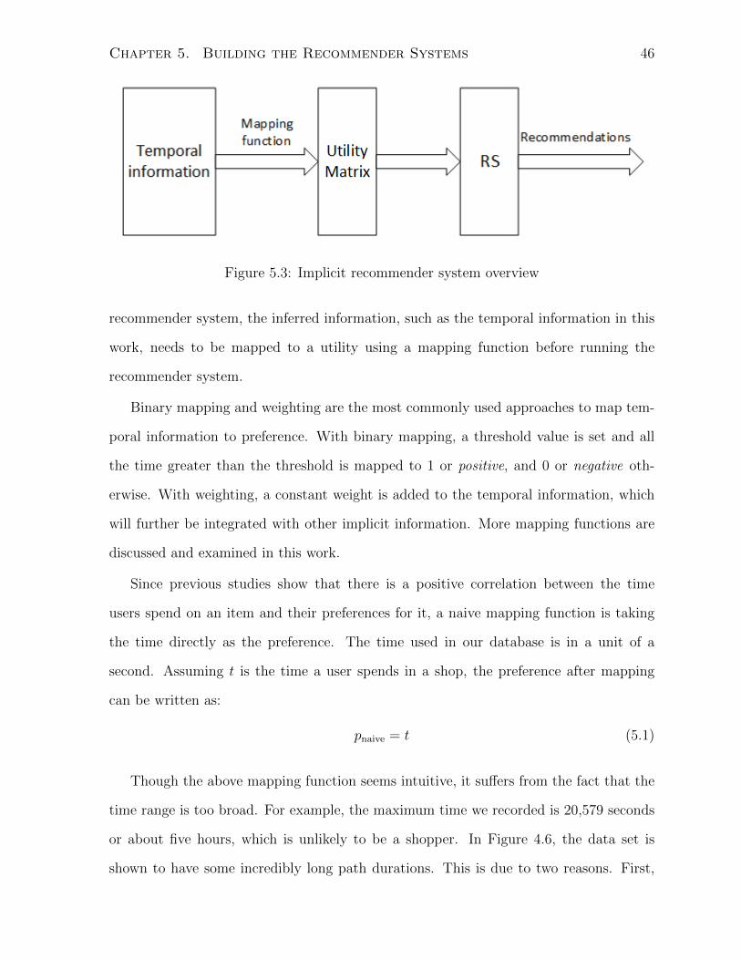
Chapter 5. Building the Recommender Systems 46
Figure 5.3: Implicit recommender system overview
recommender system, the inferred information, such as the temporal information in this
work, needs to be mapped to a utility using a mapping function before running the
recommender system.
Binary mapping and weighting are the most commonly used approaches to map tem-
poral information to preference. With binary mapping, a threshold value is set and all
the time greater than the threshold is mapped to 1 or positive, and 0 or negative oth-
erwise. With weighting, a constant weight is added to the temporal information, which
will further be integrated with other implicit information. More mapping functions are
discussed and examined in this work.
Since previous studies show that there is a positive correlation between the time
users spend on an item and their preferences for it, a naive mapping function is taking
the time directly as the preference. The time used in our database is in a unit of a
second. Assuming t is the time a user spends in a shop, the preference after mapping
can be written as:
pnaive = t (5.1)
Though the above mapping function seems intuitive, it suffers from the fact that the
time range is too broad. For example, the maximum time we recorded is 20,579 seconds
or about five hours, which is unlikely to be a shopper. In Figure 4.6, the data set is
shown to have some incredibly long path durations. This is due to two reasons. First,

Chapter 5. Building the Recommender Systems 47
it is quite possible that the MSE fails to refresh the information of certain devices over
time. Second, the devices belong to employees of the shopping mall who tend to spend
eight hours every day there. No matter which reason it is, these unreasonable data will
impact the performance of the recommender system. Therefore, any time over one hour
or 3600 seconds is assumed to be one hour. If the users do spend more than one hour
looking around a shop, that means they extremely like the shop. With such an upper
bound, the mapping function can be written as:
pub = min(3600, t) (5.2)
Equations (5.1) and (5.2) all deal with real time units, but in real applications such
as eBay and BestBuy, the preferences are always expressed in a much smaller scale. For
example, BestBuy uses the number of stars for rating, which is equivalent to a scale of 1
to 5. Therefore, it makes sense to map the time to smaller scales for a better comparison
to other works in the future. For the next two mapping functions, the time is mapped
to a scale of 0 to 6.
Two rules needs to be satisfied when developing a scaling equation. First, the final
function p = f(t) has to remain non-decreasing. Second, according to the assumption,
one hour will still be the upper bound of the real data, which means all t > 3600 will be
mapped to 6.
A simple method is to use a linear function for scaling, as shown in Equation (5.3).
This is equivalent to adding a constant weight to the temporal information. The ad-
vantage of this approach is that when incorporated with other implicit information to
generate a final preference, adding another weight to this preference will not change the
linearity.
plinear = min(6, t/600) (5.3)
However, the linear approach has its own drawbacks. As shown in Figure 4.6, the

Chapter 5. Building the Recommender Systems 48
data tend to be more intensive when t is smaller. The distribution of the time of each
point is more like a negative exponential function. Therefore, an intuitive idea is to use
a logarithmic function for mapping. The mapping equation can be written as:
pln = min(6, ln(t/10 + 1)) (5.4)
A 1 is added to the equation to make the preference positive. For t = 3600, pln is
about 5.89.
5.3.2 Evaluation metrics
Two metrics are proposed to evaluate the mapping function and recommender system
pair. The first metric is the scoring metric discussed in Section 2.2.3. Since the final
goal is to evaluate the efficiency of the recommender systems, the traditional evaluation
method for recommender systems is still essential here.
However, the scoring metric alone is far from applicable when evaluating mapping
functions with scaling such as plinear and pln in Section 5.3.1. Take a simple example.
Consider the following mapping function:
pfake = t/3600 (5.5)
With such a mapping function, most of the preferences will be mapped to near 0
with only a few points from 1 to 6. Since all the preferences are similar, the predicted
preferences given by the recommender system will be near 0 as well, which will be close
to the real preferences. So unexpectedly the performance of the recommender system
is good with the scoring metric though this mapping function is obviously not useful.
Another metric, therefore, is required to evaluate the mapping functions with scaling.
The other metric proposed is called distribution error, which literally means it deter-
mines the validity of the mapping function by examining the distribution of the resulting
ratings. Assume that all the shop owners are clever in that they are selling popular items

Chapter 5. Building the Recommender Systems 49
to make profits. However, since different customers have their own needs and tastes, some
of them will like the items while others will not, resulting in different ratings. Therefore,
if the number of customers is large enough to include all customers with different needs
and tastes, the distribution of ratings is likely to be random. Since the number of ratings
and the ratings themselves are discrete, a uniform distribution can be interpreted as a
constant number of ratings for every fixed interval of rating. For example, for a scale
of [0, 6] in our case, the probability of ratings belong to [a, a + 1) will be 17, where a is
a number between 0 and 5. The probability of p = 6 itself is 17
since it contains all the
points with t > 3600.
The distribution error metric Ed is a modified version of least square error for discrete
data. Algorithm 4 shows a pseudo code to calculate Ed. If the number of sub-ranges
in the algorithm is n, the error will be in the range [0, n−1n
]. If n→∞, the error will
be in the range[0, 1), which is equivalent to the continuous distribution. Normally the
range r is chosen to be n, resulting in a unit interval when dividing the range in Step 1
of Algorithm 4. For example, if the rating scale is 1 to 5, n will be 5, so the error will be
in the range [0, 0.8]. The closer Ed is to 0, the more random the distribution will be.
1. split the range of rating r into n sub-ranges with constant intervals rn;
2. classify different ratings into the n sub-ranges;
3. record the number of ratings in each sub-range as Ni;
4. calculate the distribution of each sub-range as pi = Ni
N, where N is the total
number of ratings;
5. calculate the least square error: Ed =n∑
i=1
(pi − 1n)2;
Algorithm 4: Distribution error metric
The well-known GroupLens [17] 1M data set is used as a example to evaluate the
distribution error metric. The GroupLens data set is derived from real users’ ratings of
movies. It consists of 1 million ratings from 6000 users on 4000 movies, each of which is

Chapter 5. Building the Recommender Systems 50
Table 5.1: GroupLens 1M breakdown
rating count probability
1 56174 5.6%
2 107557 10.8%
3 261197 26.1%
4 348971 34.9%
5 225310 22.5%
an integer number between 1 and 5. Table 5.1 presents a breakdown of each rating for
the data set. According to the distribution error metric, Ed = 0.056 in a range [0, 0.8],
which strongly supports the assumption of uniform distribution. It can be concluded
that this evaluation metric is sufficient to examine the distribution as the result is near
0.

Chapter 6
Methodology and Evaluation
This chapter shows how various experiments are set up to test both the mapping functions
and the recommender systems. The evaluation results will be provided as well as a
discussion on the results.
6.1 Methodology
This section will introduce the methodology to evaluate different kinds of recommender
systems used in this thesis. Both the hardware and software platforms will be presented.
6.1.1 Experimental platform
The platform is based on the most recent Mahout 7.0 and the most compatible Java
Development Kit (JDK) 6.0.
Though the hardware of the computing platform has no influence on the accuracy
of the recommender systems, it plays an important role in the execution time. The
software is run on a desktop with 4GB DDR3 memory and an Intel Core i5-2500, which
is a quad-core CPU running at 3.3GHz. The operating system is Ubuntu 12.10 64-bit.
51

Chapter 6. Methodology and Evaluation 52
6.1.2 Test cases
A series of user-based RSs with various numbers of neighbours, one item-based RS and
one Slope-One RS are built to compare the performance of different kinds of recommender
systems in this LBS application. Both unweighted and weighted similarity metrics are
tested in all the RSs, but only the unweighted result is shown in this thesis since the
difference is not significant.
To further evaluate the user-based RS, we build nine RSs with various numbers of
neighbours or neighbourhood sizes. Instead of enumerating all the possibilities, only
neighbourhood sizes of powers of 2 are examined: 2, 4, 8 ..., 512.
All the eleven RSs are used to test each mapping function discussed in Section 5.3,
generating a total of 44 results.
6.1.3 Evaluation methods
As discussed in Chapter 2, since the scoring evaluation metric involves random selection
of the input data, the result for each run varies. Therefore, to minimize the effect of
randomization, each case is run ten times, and an average score is taken as the final
score for the case. The scoring metric are used to evaluate the recommender system
only. Therefore, all the temporal information in the input data are first mapped to
preferences using the mapping functions. For all the testing cases, 90% of the preferences
are randomly selected as the training set. The recommender systems then use it to
predict the remaining 10% of the preferences, which is referred to as the testing set. The
score is the average absolute difference between the predicted values and the original
testing set.
Besides the scoring metric, the distribution error metric is used to evaluate the two
mapping functions with scaling.
To measure the execution time, the standard JAVA timer function System.nanoTime()

Chapter 6. Methodology and Evaluation 53
is used. It returns the current value of the most precise available system timer in nanosec-
onds.
6.2 Evaluation
This section shows the evaluation results of the experiments. Each mapping function
and recommender system pair is evaluated by the scoring metric and distribution error
metric if applicable.
6.2.1 Evaluation of non-scaling mapping functions
This section evaluates the following two non-scaling mapping functions. The time t, used
in this section, is in a unit of a second.
pnaive = t
pub = min(3600, t)
Figure 6.1 shows the correlation between scores and the number of neighbours for the
two mapping functions. For all the various neighbourhood sizes, pub outperforms pnaive.
This is because pub can efficiently filter out the abnormal points with an extraordinarily
long time. The trade-off of neighbourhood size is that with a larger number of neighbours,
the effect of counter preferences of some close neighbours will be reduced, while with a
smaller one, the close neighbours can provide a more accurate prediction in some common
preference. The best score for pnaive is achieved when the neighbourhood size is 16, with
the score being 680 seconds. The best score for pub is achieved when the neighbourhood
size is 64, with the score being 550 seconds. Therefore, the best error of the two mapping
functions used in a user-based RS is 550 seconds. In other words, when used to predict
the time a random user spends in a random shop, the RS can generate a prediction within

Chapter 6. Methodology and Evaluation 54
Figure 6.1: User-based RS with non-scaling mapping functions
nine minutes on average. The average time users spend in each location is 654s or about
11 minutes. Therefore, the recommender systems should be improved for real-world
applications as the prediction error is too significant compared to the average time.
A comparison of different kinds of RSs with the two mapping functions are shown in
Table 6.1. The differences between the three kinds of RSs are not significant. There is no
guarantee which one will outperform the others, since the performance depends highly
on how the real data matches the models. However, since each type of RS has its own
Table 6.1: Comparison of RSs with non-scaling mapping functions
RS type pnaive pub
User-based 680 550
Item-based 761 606
Slope-One 657 591

Chapter 6. Methodology and Evaluation 55
Figure 6.2: User-based RS with scaling mapping functions
assumption, it can be concluded that all the assumptions are valid to some extent in this
data set. Specifically, the Slope-One RS performs best with pnaive while the user-based
RS works best with pub. The item-based RS is slightly worse than the other two with
both algorithms.
6.2.2 Evaluation of mapping functions with scaling
This section evaluates the following two mapping functions without scaling. Both plinear
and pln are in a scale of [0, 6].
plinear = min(6, t/600)
pln = min(6, ln(t/10 + 1))

Chapter 6. Methodology and Evaluation 56
Table 6.2: Comparison of RSs with scaling mapping functions
RS type plinear pln
User-based 0.916 1.321
Item-based 1.017 1.377
Slope-One 0.994 1.292
Table 6.3: Distribution error for scaling mapping functions
plinear pln
Ed 0.636 0.178
Figure 6.2 shows the correlation between scores and the number of neighbours for
the two mapping functions. Both of plinear and pln achieve the best score when the
neighbourhood size is 32. The best score for plinear is 0.916, while for pln it is 1.321. With
a neighbourhood size ranging from 2 to 64, the scores for pln are close to each other,
indicating that the similarity between a user and each of its n neighbours is close with
this mapping function. For all the neighbourhood size, plinear outperforms pln significantly.
A comparison of different kinds of RSs is shown in Table 6.2. The user-based approach
performs the best with plinear, while the Slope-One approach is best with pln. The item-
based RS is slightly worse than the other two with both functions. Since a typical score
for the GroupLens data set is about 0.9 with a rating range [1, 5], 0.916 or 1.292 score
with a rating range [0, 6] is acceptable. Similar to the conclusion drawn from the user-
based approach, for all three RS types, plinear outperforms pln significantly. A better score
can be because that the mapping function is really good or the mapped preferences are
compressed. Therefore, the distribution error needs to be taken into consideration.
Table 6.3 presents the distribution errors Ed for both plinear and pln. The Ed is in a
range [0, 0.86]. Apparently, pln is much better than plinear in distribution error, indicating
that the pln is a more realistic mapping function. Recall that in Section 5.3.2, the Ed
of the GroupLens data set is 0.056. The pln is not ideal and can be improved in the

Chapter 6. Methodology and Evaluation 57
future. However, the pln can generate a reasonable performance with a more realistic
distribution, and is thus a better candidate for this application.
6.2.3 Execution time evaluation
Table 6.4 shows the execution time for each type of RS with the pln mapping function.
In the table, user-based (n) means user-based RS with neighbourhood size n. Each RS is
run ten times and the value presented is the total elapsed time. The execution times for
each user-based RS with different neighbourhood sizes is similar. This is simply because
building the RS requires a traversal of the whole data set regardless of the neighbourhood
size. A notable fact is that the item-based RS and Slope-One are much faster than the
user-based approach, as discussed in Chapter 2. In terms of the scalability, when the
data size grows, both the item-based and the Slope-One RS can be pre-computed so that
the online service time can be easily scaled. Therefore, in reality, a Slope-One RS is the
best choice because of its accuracy and speed.

Chapter 6. Methodology and Evaluation 58
Table 6.4: Comparison in terms of execution time
RS Ten Runs (s)
user-based (2) 16.9
user-based (4) 16.3
user-based (8) 16.2
user-based (16) 16.2
user-based (32) 16.4
user-based (64) 16.5
user-based (128) 16.8
user-based (256) 17.1
user-based (512) 17.5
item-based 0.97
Slope-One 0.39

Chapter 7
Conclusion
Indoor localization with WiFi is demonstrating a great potential to increase business
value of the network infrastructures. CISCO has realized the goal of indoor localization
by integrating the MSE into their network infrastructure. However, the tracks collected
by such a system are never studied in spite of its great potential values. This work
aims at analysing the tracks collected from the Bow Valley shopping mall and building
a recommender system for the shopping mall.
The time a user spends in a shop is taken as an implicit preference. Different mapping
algorithms to process the implicit preference are proposed and evaluated in this thesis.
In addition to the traditional scoring metric, we propose using the distribution error as
another metric to evaluate the mapping algorithms.
Eleven recommender systems are built to determine the best one for our application:
nine user-based approaches with various neighbourhood sizes, one item-based approach
and one Slope-One approach. Each recommender system with a certain mapping algo-
rithm is examined in terms of scoring metric, distribution error and execution time. The
Slope-One recommender system with the pln mapping algorithm is finally selected in our
application with a score of 1.292, distribution error of 0.178 and execution time of 0.39
seconds for ten runs.
59

Chapter 8
Future Work
This work only shows our first attempt in finding a suitable recommender system based
on indoor localization tracks. Though we tried our best to cover all the possible solutions,
there are still many directions that we can go in the future.
The first one is to find a better similarity metric. The Pearson correlation-based
similarity is the only metric we are using in this thesis. However, other metrics such
as Spearman correlation-based or Tanimoto coefficient-based similarity metrics are also
good candidates to our application.
Another one is to evaluate the scalability of the recommender systems. The data set
we are using in this thesis is collected for one week with a size of about 500MB. It is
expected that in reality a much larger data set will be used. Therefore, running it on
a high performance distributed computing system such as Hadoop or using customized
accelerators such as Graphic Processing Units (GPU) or Field Programmable Gate Arrays
(FPGAs) will be a very interesting topic in the future.
The third possibility will be to explore other mapping algorithms. First, the preference
can be mapped to binary numbers. For example, if a user has been to a shop, then
the preference is 1, otherwise 0. Though this approach will lose some details, it can
probably provide better performance, since people tend to only go to the shops they like.
60

Chapter 8. Future Work 61
Second, when developing the distribution error metric, we make the assumption that the
distribution in the real world is uniform. However, it may not be necessary since most
people do not give extremely high or extremely low ratings. Therefore, it is quite possible
that a normal distribution can be a better prediction.
As the goal of the current work is to determine the feasibility of building a recom-
mender system for MSE positioning systems, only widely-used and simple recommender
system algorithms are tested. Another test bed with an AP configuration for positioning
will be built and after that more sophisticated algorithms will be explored to develop a
better recommendation system. For example, the singular value decomposition (SVD),
a well-known method for matrix factorization that can be used to reduce the dimension-
ality of sparse ratings matrices, is proved to achieve better performance than traditional
collaborative filtering algorithms [38]. The Support Vector Machine (SVM) is concep-
tually suitable for classification problems and could be possibly used in a model-based
recommender system. Though the SVM is known to perform poorly for collaborative
filtering in a model-based recommender system due to extremely unbalanced class dis-
tributions [39], it can be implemented with user-based recommender systems when more
contexts are available [40].

Bibliography
[1] G. Adomavicius and A. Tuzhilin. Toward the next generation of recommender sys-
tems: a survey of the state-of-the-art and possible extensions. Knowledge and Data
Engineering, IEEE Transactions on, 17(6):734–749, 2005.
[2] Sean Owen, Robin Anil, Ted Dunning, and Ellen Friedman. Mahout in action, 2010.
[3] CISCO. Context-Aware Mobility (Location) API, 2013. URL: http://developer.
cisco.com/web/contextaware/resources.
[4] Minority Report, 2013. URL: http://www.youtube.com/watch?v=uiDMlFycNrw.
[5] Peter Ljungstrand. Context awareness and mobile phones. Personal Ubiquitous
Comput., 5(1):58–61, January 2001.
[6] Axel Kpper. Indoor Positioning, pages 233–245. John Wiley and Sons, Ltd, 2005.
[7] Thomas P. Moran and Paul Dourish. Introduction to this special issue on context-
aware computing. HumanComputer Interaction, 16(2-4):87–95, 2001.
[8] Hofmann-Wellenhof, B. Lichtenegger, H. Collins, J. Springer, and Wien (Austria).
Global Positioning System. Theory and practice. 1993.
[9] Apple Acquires Indoor GPS Startup WiFiSlam, 2013. URL: http://techcrunch.
com/2013/03/24/apple-acquires-indoor-gps-startup-wifislam-for-20m/.
62

Bibliography 63
[10] Cisco Announces Acquisition of ThinkSmart, 2012. URL: http://www.cisco.com/
web/about/ac49/ac0/ac1/ac259/thinksmart.html.
[11] Raphael Leiteritz. Copy of Google’s submission to several national data protection
authorities on vehicle-based collection of WiFi data for use in Google Location
based services, 2010. URL: http://static.googleusercontent.com/external_
content/untrusted_dlcp/www.google.com/en//googleblogs/pdfs/google_
submission_dpas_wifi_collection.pdf.
[12] Francesco Ricci, Lior Rokach, Bracha Shapira, and Paul B. Kantor. Recommender
Systems Handbook. 2011.
[13] Qi Liu, Haiping Ma, Enhong Chen, and Hui Xiong. A survey of context-aware mobile
recommendations. International Journal of Information Technology and Decision
Making, 12(01):139–172, 2013.
[14] Jeffrey D. Ullman Anand Rajaraman, Jure Leskovec. Mining of massive datasets,
2013. URL: http://infolab.stanford.edu/~ullman/mmds.html#latest.
[15] Bow Valley Square, 2013. URL: http://bowvalleysquare.com/directory/.
[16] Upendra Shardanand and Pattie Maes. Social information filtering: algorithms for
automating word of mouth. In Proceedings of the SIGCHI Conference on Human
Factors in Computing Systems, CHI ’95, pages 210–217, New York, NY, USA, 1995.
ACM Press/Addison-Wesley Publishing Co.
[17] Paul Resnick, Neophytos Iacovou, Mitesh Suchak, Peter Bergstrom, and John Riedl.
Grouplens: an open architecture for collaborative filtering of netnews. In Proceedings
of the 1994 ACM conference on Computer supported cooperative work, CSCW ’94,
pages 175–186, New York, NY, USA, 1994. ACM.

Bibliography 64
[18] Will Hill, Larry Stead, Mark Rosenstein, and George Furnas. Recommending and
evaluating choices in a virtual community of use. In Proceedings of the SIGCHI
Conference on Human Factors in Computing Systems, CHI ’95, pages 194–201, New
York, NY, USA, 1995. ACM Press/Addison-Wesley Publishing Co.
[19] Gediminas Adomavicius and Alexander Tuzhilin. Context-aware recommender sys-
tems. In Francesco Ricci, Lior Rokach, Bracha Shapira, and Paul B. Kantor, editors,
Recommender Systems Handbook, pages 217–253. Springer US, 2011.
[20] Amazon Book Department, 2013. URL: http://www.amazon.ca.
[21] BestBuy, 2013. URL: http://www.bestbuy.ca/en-CA/category/
laptops-ultrabooks/20352opt.aspx.
[22] Marko Balabanovic and Yoav Shoham. Fab: content-based, collaborative recom-
mendation. Commun. ACM, 40(3):66–72, March 1997.
[23] Masahiro Morita and Yoichi Shinoda. Information filtering based on user behavior
analysis and best match text retrieval. In Proceedings of the 17th annual interna-
tional ACM SIGIR conference on Research and development in information retrieval,
SIGIR ’94, pages 272–281, New York, NY, USA, 1994. Springer-Verlag New York,
Inc.
[24] John S. Breese, David Heckerman, and Carl Kadie. Empirical analysis of predictive
algorithms for collaborative filtering. In Proceedings of the Fourteenth conference on
Uncertainty in artificial intelligence, UAI’98, pages 43–52, San Francisco, CA, USA,
1998. Morgan Kaufmann Publishers Inc.
[25] Anna Maclachlan Daniel Lemire. Slope one predictors for online rating-based col-
laborative filtering. SDM’05, 2005.

Bibliography 65
[26] S. Sae-Ueng, S. Pinyapong, A. Ogino, and T. Kato. Consumer-friendly shopping
assistance by personal behavior log analysis on ubiquitous shop space. In Asia-
Pacific Service Computing Conference, The 2nd IEEE, pages 496–503, 2007.
[27] Chun-Nan Hsu, Hao-Hsiang Chung, and Han-Shen Huang. Mining skewed and
sparse transaction data for personalized shopping recommendation. Machine Learn-
ing, 57(1-2):35–59, 2004.
[28] A. Asthana, M. Cravatts, and P. Krzyzanowski. An indoor wireless system for
personalized shopping assistance. In Mobile Computing Systems and Applications,
1994. Proceedings., Workshop on, pages 69–74, 1994.
[29] F. von Reischach, D. Guinard, F. Michahelles, and E. Fleisch. A mobile product
recommendation system interacting with tagged products. In Pervasive Comput-
ing and Communications, 2009. PerCom 2009. IEEE International Conference on,
pages 1–6, 2009.
[30] Ricardo Anacleto, Nuno Luz, Ana Almeida, Lino Figueiredo, and Paulo Novais.
Shopping center tracking and recommendation systems. In Emilio Corchado, Vclav
Snel, Javier Sedano, AboulElla Hassanien, JosLuis Calvo, and Dominik lzak, edi-
tors, Soft Computing Models in Industrial and Environmental Applications, 6th In-
ternational Conference SOCO 2011, volume 87 of Advances in Intelligent and Soft
Computing, pages 299–308. Springer Berlin Heidelberg, 2011.
[31] Wei-Jen Hsu. Behavioral analysis, user modeling, and protocol design based on
large-scale wireless network traces. Master’s thesis, University of Florida, 2008.
[32] Lauri Aalto, Nicklas Gothlin, Jani Korhonen, and Timo Ojala. Bluetooth and wap
push based location-aware mobile advertising system. In Proceedings of the 2nd
international conference on Mobile systems, applications, and services, MobiSys ’04,
pages 49–58, New York, NY, USA, 2004. ACM.
Bibliography 66
[33] Gregory D. Abowd, Christopher G. Atkeson, Jason Hong, Sue Long, Rob Kooper,
and Mike Pinkerton. Cyberguide: a mobile context-aware tour guide. Wirel. Netw.,
3(5):421–433, October 1997.
[34] Quannan Li, Yu Zheng, Xing Xie, Yukun Chen, Wenyu Liu, and Wei-Ying Ma.
Mining user similarity based on location history. In Proceedings of the 16th ACM
SIGSPATIAL international conference on Advances in geographic information sys-
tems, GIS ’08, pages 34:1–34:10, New York, NY, USA, 2008. ACM.
[35] Kyoung-jae Kim Hyunchul Ahn and Ingoo Han. Mobile Advertisement Recom-
mender System using Collaborative Filtering: MAR-CF. In Proceeding of The Korea
Society of Management Information Systems, 2006.
[36] CISCO. Cisco Mobility Services Engine Data Sheet, 2013. URL:
http://www.cisco.com/en/US/prod/collateral/wireless/ps9733/ps9742/
data_sheet_c78-475378.html.
[37] Yifan Hu, Y. Koren, and C. Volinsky. Collaborative filtering for implicit feedback
datasets. In Data Mining, 2008. ICDM ’08. Eighth IEEE International Conference
on, pages 263–272, 2008.
[38] Daniel Billsus and Michael J. Pazzani. Learning collaborative inforamtion filters. In
International Conference on Machine Learning, 1998.
[39] Tong Zhang and Vijay S. Iyengar. Recommender systems using linear classifiers. J.
Mach. Learn. Res., 2:313–334, March 2002.
[40] K. Oku, S. Nakajima, J. Miyazaki, and S. Uemura. Context-aware svm for context-
dependent information recommendation. In Mobile Data Management, 2006. MDM
2006. 7th International Conference on, pages 109–109, 2006.