PNNL-13435

Indoor Air Nuclear, Biological, and Chemical Health Modeling and Assessment System R. D. Stenner J. W. Buck D. L. Hadley B. L. Hoopes P. R. Armstrong M. C. Janus March 2001 Prepared for the U.S. Department of Energy under Contract DE-AC06-76RL01830

DISCLAIMER This report was prepared as an account of work sponsored by an agency of the United States Government. Neither the United States Government nor any agency thereof, nor Battelle Memorial Institute, nor any of their employees, makes any warranty, express or implied, or assumes any legal liability or responsibility for the accuracy, completeness, or usefulness of any information, apparatus, product, or process disclosed, or represents that its use would not infringe privately owned rights. Reference herein to any specific commercial product, process, or service by trade name, trademark, manufacturer, or otherwise does not necessarily constitute or imply its endorsement, recommendation, or favoring by the United States Government or any agency thereof, or Battelle Memorial Institute. The views and opinions of authors expressed herein do not necessarily state or reflect those of the United States Government or any agency thereof. PACIFIC NORTHWEST NATIONAL LABORATORY operated by BATTELLE for the UNITED STATES DEPARTMENT OF ENERGY under Contract DE-AC06-76RL01830

This document was printed on recycled paper.

(8/00)

PNNL-13435

Indoor Air Nuclear, Biological, and Chemical Health Modeling and Assessment System R. D. Stenner J. W. Buck D. L. Hadley B. L. Hoopes P. R. Armstrong M. C. Janus March 2001 Prepared for the U.S. Department of Energy under Contract DE-AC06-76RL01830 Pacific Northwest National Laboratory Richland, Washington 99352

iii

Summary Indoor air quality effects on human health are of increasing concern to public health agencies and building owners. The prevention and treatment of ‘sick building’ syndrome and the spread of air-borne diseases in hospitals, for example, are well known priorities. However, increasing attention is being directed to the vulnerability of public buildings and places, public security, and national defense facilities to terrorist attack or the accidental release of airborne biological pathogens, harmful chemicals, or radioactive contaminants. The Indoor Air Nuclear, Biological, and Chemical Health Modeling and Assessment System (IA-NBC-HMAS) was developed to serve as a health impact analysis tool for use in addressing these concerns. The overall goals were (a) to develop a user-friendly fully functional prototype health modeling and assessment system, which will operate under the Pacific Northwest National Laboratory (PNNL) Framework for Risk Analysis in Multimedia Environmental Systems (FRAMES) for ease of use and (b) to maximize its integration with other modeling and assessment capabilities accessible within the FRAMES system (e.g., ambient air fate and transport models, water-borne fate and transport models, physiologically based pharmacokinetic models, etc.). This prototype system was developed as an internally funded Laboratory Directed Research and Development (LDRD) project, which was completed over a two-year period in fiscal years 2000 and 2001. The prototype IA-NBC-HMAS is designed to serve as a functional health modeling and assess-ment system that can be easily tailored to meet specific building analysis needs of a customer. The prototype system was developed and tested using an actual building (i.e., the Churchville Building located at the Aberdeen Proving Ground) and release scenario (i.e., the release and measurement of tracer materials within the building) to ensure realism and practicality in the design and development of the prototype system. A user-friendly “demo” accompanies this report to allow the reader the opportunity for a “hands on” review of the prototype system’s capability. The “demo” was developed to function as a stand-alone executable file for demonstration purposes. However, the actual IA-NBC-HMAS operates under the PNNL-developed FRAMES system for more flexibility and linking with other models and assessment systems, such as ambient air analysis models, toxicokinetic models, etc., for complete analysis of the system of scenarios that would normally be associated with a terrorist attack on a building. However, the IA-NBC-HMAS will operate very efficiently by itself within the FRAMES system for use in “what if” analyses for building planning and emergency response planning purposes.

v

Acronyms BHED Biological Health Effect Database CBNP Chemical and Biological Nonproliferation Program CFD computational fluid dynamics CHED Chemical Health Effects Database DOE Department of Energy DOD Department of Defense DTRA Defense Threat Reduction Agency FEMA Federal Emergency Management Agency FRAMES Framework for Risk Analysis in Multimedia Environmental Systems HVAC heating, ventilation, and air conditioning IA-NBC-HMAS Indoor Air Nuclear, Biological, and Chemical Health Modeling and Assessment System IAQ indoor air quality LDRD Laboratory Directed Research and Development NBC nuclear, biological, and chemical NGA National Governors’ Association PNNL Pacific Northwest National Laboratory VA vulnerability assessment

vii

Acknowledgments The Indoor Air Nuclear, Biological, and Chemical Health Modeling and Assessment System was developed as a Laboratory Directed Research and Development (LDRD) project. The aim of the LDRD program is to foster the development of new or expanding capabilities. The authors wish to acknowledge and thank Dennis Strenge for providing peer review and technical review support for the development of this report.

ix

Contents Summary.................................................................................................................................. iii Acronyms ................................................................................................................................ v Acknowledgments .................................................................................................................... vii 1.0 Introduction ...................................................................................................................... 1.1 1.1 Threat from Chemical and Biological Agents............................................................... 1.1 1.2 Preparedness and Threat Reduction............................................................................ 1.2 2.0 Model and Modeling.......................................................................................................... 2.1 2.1 Building Airflow Models............................................................................................. 2.1 2.2 Dispersion Model of Churchville Test Building............................................................. 2.4 2.3 Whole-Building Airflow Network Characterization by Inverse Modeling........................ 2.7 3.0 Dose Calculation Routine................................................................................................... 3.1 3.1 Chemical Agent Dose Calculation Equation................................................................. 3.1 3.2 Biological Agent Dose Calculation Equation ................................................................ 3.1 4.0 Health Effect Databases ................................................................................................... 4.1 5.0 Integration into FRAMES.................................................................................................. 5.1 6.0 Output Design................................................................................................................... 6.1 7.0 Prototype IA-NBC-HMAS Demonstration ......................................................................... 7.1 8.0 References ...................................................................................................................... 8.1 Appendix A - Whole-Building Airflow Network Characterization by Inverse Modeling.................. A.1 Appendix B - Newton-Raphson Application Details .................................................................... B.1 Appendix C - Example Biological Health Effect Database for Biological Agents........................... C.1 Appendix D - Example Chemical Health Effect Database for Chemical Agents............................ D.1

x

Figures 1.1 Overall IA-NBC-HMAS Design........................................................................................ 1.1 2.1 Illustration of the CONTAM Process of Identifying Building Zones and Resultant

Air Flows ...................................................................................................................... 2.4 2.2 Churchville Test Facility..................................................................................................... 2.5 2.3 CONTAM Sketchpad Rendering of the First Floor of the Churchville Test Facility ................ 2.6 2.4 Measured and Simulated Concentration Histories ................................................................ 2.6 5.1 FRAMES Graphic Layout of Conceptual Model of the Example Churchville Building Analysis ............................................................................................................... 5.1 5.2 First-Floor Layout of the Example Churchville Building........................................................ 5.2 6.1 Example IA-NBC-HMAS Health Effect/Symptom Output Table ......................................... 6.1

Table 2.1 Summary of Building Dispersion Model Characteristics ....................................................... 2.2

1.1

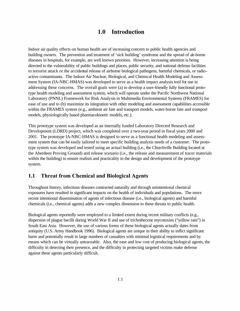
1.0 Introduction Indoor air quality effects on human health are of increasing concern to public health agencies and building owners. The prevention and treatment of ‘sick building’ syndrome and the spread of air-borne diseases in hospitals, for example, are well known priorities. However, increasing attention is being directed to the vulnerability of public buildings and places, public security, and national defense facilities to terrorist attack or the accidental release of airborne biological pathogens, harmful chemicals, or radio-active contaminants. The Indoor Air Nuclear, Biological, and Chemical Health Modeling and Assess-ment System (IA-NBC-HMAS) was developed to serve as a health impact analysis tool for use in addressing these concerns. The overall goals were (a) to develop a user-friendly fully functional proto-type health modeling and assessment system, which will operate under the Pacific Northwest National Laboratory (PNNL) Framework for Risk Analysis in Multimedia Environmental Systems (FRAMES) for ease of use and to (b) maximize its integration with other modeling and assessment capabilities accessible within the FRAMES system (e.g., ambient air fate and transport models, water-borne fate and transport models, physiologically based pharmacokinetic models, etc.). This prototype system was developed as an internally funded Laboratory Directed Research and Development (LDRD) project, which was completed over a two-year period in fiscal years 2000 and 2001. The prototype IA-NBC-HMAS is designed to serve as a functional health modeling and assess-ment system that can be easily tailored to meet specific building analysis needs of a customer. The proto-type system was developed and tested using an actual building (i.e., the Churchville Building located at the Aberdeen Proving Ground) and release scenario (i.e., the release and measurement of tracer materials within the building) to ensure realism and practicality in the design and development of the prototype system.

1.1 Threat from Chemical and Biological Agents Throughout history, infectious diseases contracted naturally and through unintentional chemical exposures have resulted in significant impacts on the health of individuals and populations. The more recent intentional dissemination of agents of infectious disease (i.e., biological agents) and harmful chemicals (i.e., chemical agents) adds a new complex dimension to these threats to public health. Biological agents reportedly were employed to a limited extent during recent military conflicts (e.g., dispersion of plague bacilli during World War II and use of trichothecene mycotoxins (“yellow rain”) in South East Asia. However, the use of various forms of these biological agents actually dates from antiquity (U.S. Army Handbook 1996). Biological agents are unique in their ability to inflict significant harm and potentially result in large numbers of casualties with minimal logistical requirements and by means which can be virtually untraceable. Also, the ease and low cost of producing biological agents, the difficulty in detecting their presence, and the difficulty in protecting targeted victims make defense against these agents particularly difficult.

1.2

Chemical agents, in the modern sense, were first used in World War I when chlorine gas was intentionally released as a warfare agent. Since World War II, there have been several confirmed reports that chemical agents have been used in armed conflicts, including the Iran-Iraq conflict (U.S. Army Handbook 1996). Like biological agents, many chemical agents are also relatively easy to obtain and can be disseminated with relative ease. They can also be difficult to detect and can be disseminated by means that are difficult to trace. In a report to Congress, the Department of Defense (DOD) states that, within the last five years, at least eleven states as well as other nations have experienced terrorist incidents (e.g., World Trade Center bombing, chemical attack on the Tokyo Subway, Oklahoma City bombing, and bombing in Centennial Park during the Olympics). With the increasing availability of raw materials and technology from worldwide sources, the potential use of weapons of mass destruction (which includes chemical and biological agents) by subversive groups has mounted dramatically (DOD 1997). The National Governors’ Association (NGA), in their 1996 workshop, stated that the states did not have adequate resources or training in the arena of chemical and biological terrorism. The NGA also indicated the need for more resources to be made available to combat chemical or biological attacks and for Federal assistance in the areas of monitoring and detection, technical assistance, manpower and recovery efforts (DOD 1997). In their September 1996 meeting, the Federal Emergency Management Agency (FEMA) identified the need for subject matter experts that can provide advice and reference materials delineating the hazards, effects and recommended protective response actions, for their response to chemical or biological agent attacks (DOD 1997). One of the significant needs identified by these various groups and by Congress is the need for adequate tools and training for the “first responders.” In recognition of this significant problem, and in response to Title 50, Subchapter 1 (“Domestic Preparedness”), the DOD has taken on the responsibility of assisting Federal, state and local officials to equip them for responding to threats involving chemical and biological weapons or related materials or technologies. As part of this overall DOD effort, the new Defense Threat Reduction Agency (DTRA) has identified “Counterproliferation” as one of its three primary mission areas. Deputy Secretary of Defense Hamre has remarked that, “the U.S. government, for the most part, has no biological weapons intellectual infrastructure, and that it should be built into the DTRA mission area because of the high potential for a chemical or biological terrorist attack on the continental U.S. sometime in the next decade or two.” He announced the concept of “Homeland Defense,” with respect to chemical and biological terrorist attacks, and included it under the rubric of “Counterproliferation.” Deputy Secretary Hamre called “consequence management” (i.e., dealing with the after-effects of a chemical or biological terrorist attach), the highest priority under “Counterproliferation.”

1.2 Preparedness and Threat Reduction In responding to a building under a chemical or biological agent attack by terrorists, there are two very important questions that need immediate answers: What has been released? and Where has it spread? The answers to these questions form the basis for determining the remaining actions of the “first responders.” Being prepared to answer these and the host of questions that follow them is essential for adequate management of the threat situation (i.e., reducing the threat through knowledge and planning).

1.3

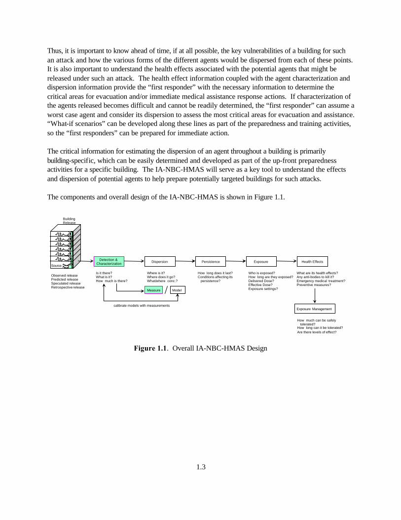
Thus, it is important to know ahead of time, if at all possible, the key vulnerabilities of a building for such an attack and how the various forms of the different agents would be dispersed from each of these points. It is also important to understand the health effects associated with the potential agents that might be released under such an attack. The health effect information coupled with the agent characterization and dispersion information provide the “first responder” with the necessary information to determine the critical areas for evacuation and/or immediate medical assistance response actions. If characterization of the agents released becomes difficult and cannot be readily determined, the “first responder” can assume a worst case agent and consider its dispersion to assess the most critical areas for evacuation and assistance. “What-if scenarios” can be developed along these lines as part of the preparedness and training activities, so the “first responders” can be prepared for immediate action. The critical information for estimating the dispersion of an agent throughout a building is primarily building-specific, which can be easily determined and developed as part of the up-front preparedness activities for a specific building. The IA-NBC-HMAS will serve as a key tool to understand the effects and dispersion of potential agents to help prepare potentially targeted buildings for such attacks. The components and overall design of the IA-NBC-HMAS is shown in Figure 1.1.

Figure 1.1. Overall IA-NBC-HMAS Design

Detection &Characterization

Dispersion Persistence Health EffectsExposure

Exposure Management

Is it there?What is it?How much is there?

Where is it?Where does it go?What/where conc.?

Measure Model

calibrate models with measurements

How long does it last?Conditions affecting its persistence?

What are its health effects?Any anti-bodies to kill it?Emergency medical treatment?Preventive measures?

Who is exposed?How long are they exposed?Delivered Dose?Effective Dose?Exposure settings?

How much can be safely tolerated?How long can it be tolerated?

Are there levels of effect?

BuildingRelease

Observed releasePredicted releaseSpeculated releaseRetrospective release

Source

2.1

2.0 Model and Modeling In order to address some of the “missing pieces” in the development of the integrated IA-NBC-HMAS tool, the following indoor air modeling subtasks were completed:

• demonstrate the ability of existing indoor air quality (IAQ) building dispersion models to predict dispersion of nuclear, biological, and chemical (NBC) simulants

• develop a test/analysis protocol for inverse modeling of building air movement.

2.1 Building Airflow Models Transport modeling of chemical/biological agents in buildings, in the near-building environment, and in the urban/regional environment is a complex issue requiring a suite of models, depending on the spatial scale of phenomenon of interest. No single model is available (nor will their ever likely be one) to address all scales. The problem can be divided into four different scales, or applications:

• transport and dispersion in a single zone in a building

• interzonal transport between multiple zones in a building and transport in/out of a single building

• near-building, single building, and arrays of a few buildings

• urban to regional mesoscale transport. Table 2.1 identifies some of the commonly used models. The choice of model depends on the release point and strength of the source and the intended application of the model. The problem of wind- and thermal-driven air movements must be addressed at all scales. The activity (diffusion, deposition and resuspension, adsorption and desorption, reactions, etc.) of contaminants must also be addressed at all scales. Computational fluid dynamics (CFD) models usually simulate air movement and contaminant dispersion simultaneously. Zonal models usually solve the air movement problem first and then evaluate contaminant dispersion in a second step. CFD models are used in analyzing the internal environment of large spaces, such as atriums, theaters, or coliseums. Such are capable of simulating the stratification of air in a conditioned environment and the diffusion of contaminants in that environment. For this project, CONTAM was selected as the multizone model. Application of the multizone model requires specification of a complete air network model. Definition of the zone and airflow path parame-ters represents the overwhelming bulk of model setup. The parameters must describe all envelope

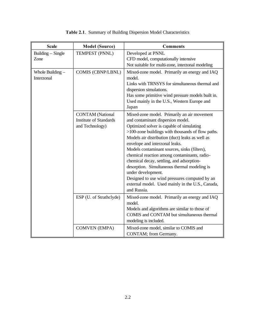
2.2

Table 2.1. Summary of Building Dispersion Model Characteristics

Scale Model (Source) Comments

Building – Single Zone

TEMPEST (PNNL) Developed at PNNL CFD model, computationally intensive Not suitable for multi-zone, interzonal modeling

COMIS (CBNP/LBNL) Mixed-zone model. Primarily an energy and IAQ model. Links with TRNSYS for simultaneous thermal and dispersion simulations. Has some primitive wind pressure models built in. Used mainly in the U.S., Western Europe and Japan

CONTAM (National Institute of Standards and Technology)

Mixed-zone model. Primarily an air movement and contaminant dispersion model. Optimized solver is capable of simulating >100-zone buildings with thousands of flow paths. Models air distribution (duct) leaks as well as envelope and interzonal leaks. Models contaminant sources, sinks (filters), chemical reaction among contaminants, radio-chemical decay, settling, and adsorption-desorption. Simultaneous thermal modeling is under development. Designed to use wind pressures computed by an external model. Used mainly in the U.S., Canada, and Russia.

ESP (U. of Strathclyde) Mixed-zone model. Primarily an energy and IAQ model. Models and algorithms are similar to those of COMIS and CONTAM but simultaneous thermal modeling is included.

Whole Building – Interzonal

COMVEN (EMPA) Mixed-zone model, similar to COMIS and CONTAM; from Germany.

2.3

Table 2.1. (contd)

Scale Model (Source) Comments FEM3 (CBNP/LLNL) CFD model requiring super-computer

computational resources. Massively parallel version being developed. Capable of high resolution flow and agent dispersion in complex flow around a single building or a few-building complex Can be scaled from fine grid resolution around a single building to a coarser grid resolution for a multi-building complex Uses a finite-element approach to simulate the mean flow with the turbulence modeled Under development, not fully operational

Near Building – Near Source

HIGRID (CBNP/LANL)

CFD model runs best in parallel-computing mode. Turn-around time on a workstation can be one week; on a super-computer, a few hours. Large-eddy simulation (LES) model with the small scales of turbulence modeled. Thus, can estimate concentration fluctuations and peak concentrations Many-building model, applies to a larger spatial domain than FEM3 Has submodules (e.g., surface energy budget) to treat important meteorological processes Does not model building interiors Under development, not fully operational

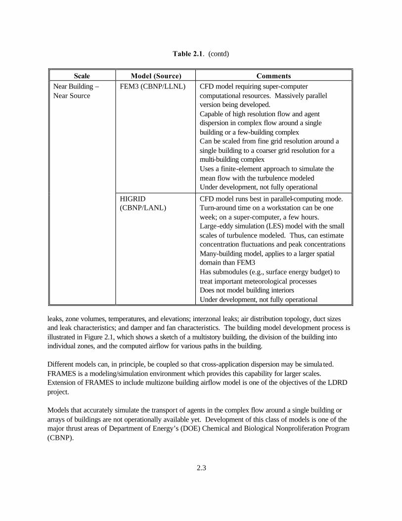
leaks, zone volumes, temperatures, and elevations; interzonal leaks; air distribution topology, duct sizes and leak characteristics; and damper and fan characteristics. The building model development process is illustrated in Figure 2.1, which shows a sketch of a multistory building, the division of the building into individual zones, and the computed airflow for various paths in the building. Different models can, in principle, be coupled so that cross-application dispersion may be simulated. FRAMES is a modeling/simulation environment which provides this capability for larger scales. Extension of FRAMES to include multizone building airflow model is one of the objectives of the LDRD project. Models that accurately simulate the transport of agents in the complex flow around a single building or arrays of buildings are not operationally available yet. Development of this class of models is one of the major thrust areas of Department of Energy’s (DOE) Chemical and Biological Nonproliferation Program (CBNP).

2.4

Figure 2.1. Illustration of the CONTAM Process of Identifying Building Zones (top) and Resultant Air

Flows (bottom)

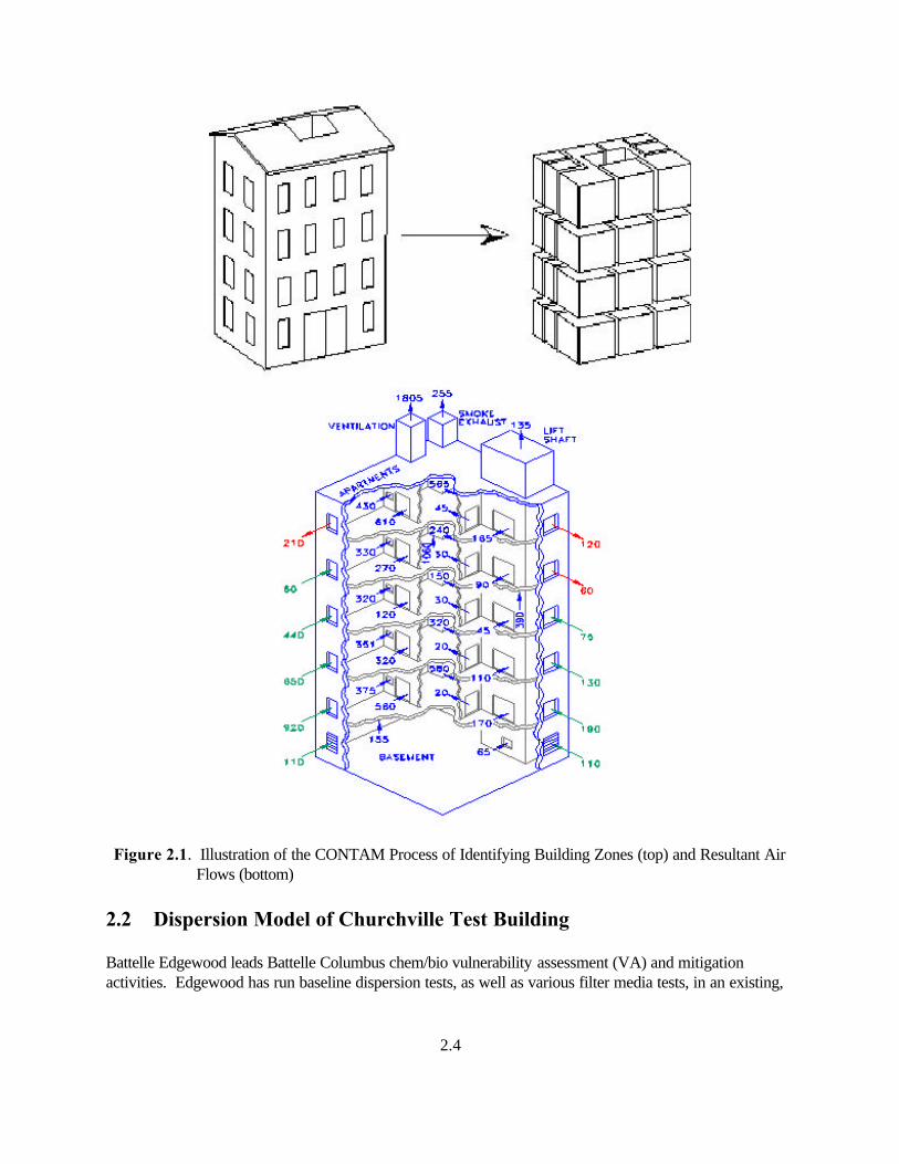
2.2 Dispersion Model of Churchville Test Building Battelle Edgewood leads Battelle Columbus chem/bio vulnerability assessment (VA) and mitigation activities. Edgewood has run baseline dispersion tests, as well as various filter media tests, in an existing,

2.5

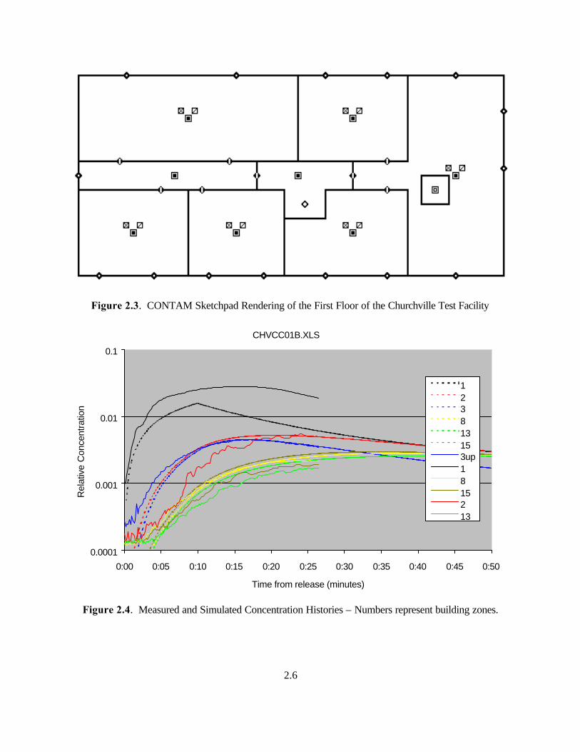
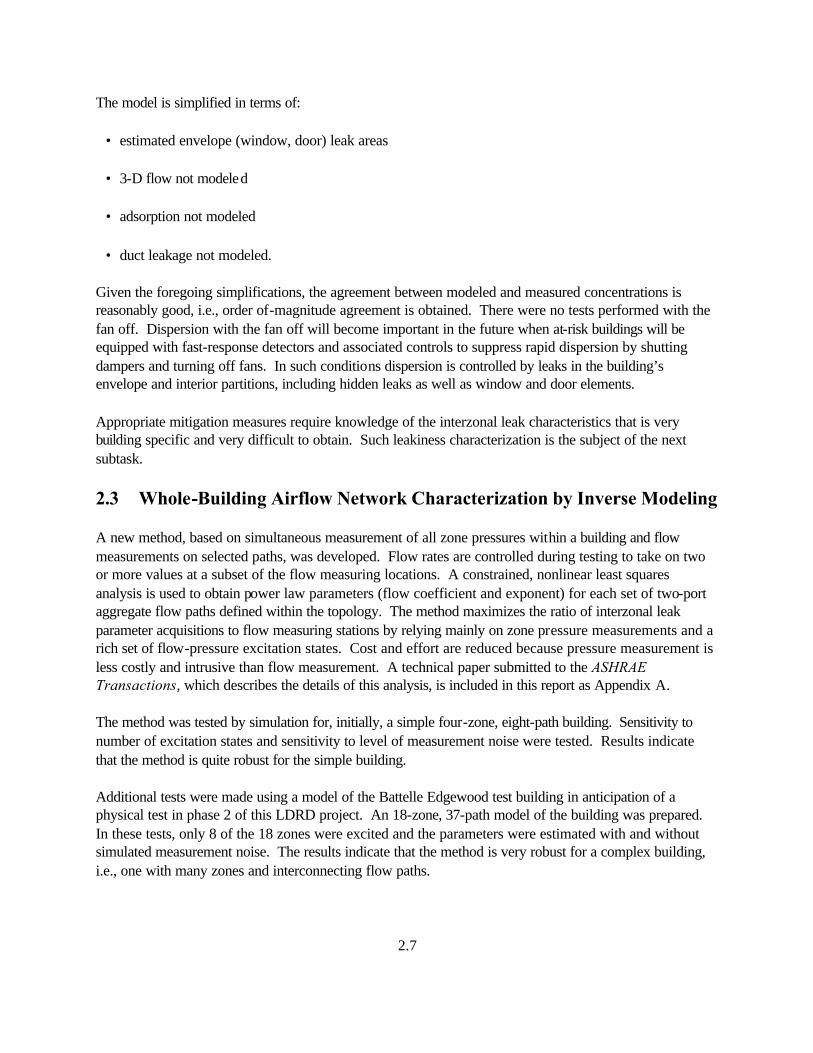
federal-client owned two-story building in Maryland (Figure 2.2). The building is heated and cooled by a single heat pump system consisting of an outdoor compressor/condenser unit and an indoor evaporator/blower unit. Airflows were measured prior to the execution of contaminant dispersion tests. Supply and return airflows were measured at the ceiling registers in each room. During operation of the heating, ventilation, and air conditioning (HVAC) fan, the dispersion rates are dominated by HVAC airflows that effectively cause air from all zones to become mixed at rates determined approximately by room air-change rates. In general, each room has a different air-change rate given by the ratio of room volume to the larger of the supply or return airflow rates. The baseline test was selected for this modeling exercise because validated adsorbing filter models are not yet available. The baseline test was made with the fan on and the outside air intake blocked. Salicylic acid, a good simulant of certain condensable chemical agents, was vaporized over a 10-minute interval in room #1. Sensors were deployed in rooms 1, 2, 3, 8, 13, and 15 to monitor simulant concentrations. The building’s floor plans are shown in the CONTAM “sketch pad” renderings (Figure 2.3). The measured and simulated concentration histories during initial buildup and decay, a 50-minute period, are shown in Figure 2.4. The model is rigorous in terms of:

• accurate room volumes and door openings

• accurate room supply and return flow rates.

Figure 2.2. Churchville Test Facility

2.6

Figure 2.3. CONTAM Sketchpad Rendering of the First Floor of the Churchville Test Facility

CHVCC01B.XLS

0.0001

0.001

0.01

0.1

0:00 0:05 0:10 0:15 0:20 0:25 0:30 0:35 0:40 0:45 0:50

Time from release (minutes)

Rela

tive C

once

ntr

atio

n

1

23

8

13

153up

1

8

152

13

Figure 2.4. Measured and Simulated Concentration Histories – Numbers represent building zones.

2.7

The model is simplified in terms of:

• estimated envelope (window, door) leak areas

• 3-D flow not modeled

• adsorption not modeled

• duct leakage not modeled. Given the foregoing simplifications, the agreement between modeled and measured concentrations is reasonably good, i.e., order of-magnitude agreement is obtained. There were no tests performed with the fan off. Dispersion with the fan off will become important in the future when at-risk buildings will be equipped with fast-response detectors and associated controls to suppress rapid dispersion by shutting dampers and turning off fans. In such conditions dispersion is controlled by leaks in the building’s envelope and interior partitions, including hidden leaks as well as window and door elements. Appropriate mitigation measures require knowledge of the interzonal leak characteristics that is very building specific and very difficult to obtain. Such leakiness characterization is the subject of the next subtask.

2.3 Whole-Building Airflow Network Characterization by Inverse Modeling A new method, based on simultaneous measurement of all zone pressures within a building and flow measurements on selected paths, was developed. Flow rates are controlled during testing to take on two or more values at a subset of the flow measuring locations. A constrained, nonlinear least squares analysis is used to obtain power law parameters (flow coefficient and exponent) for each set of two-port aggregate flow paths defined within the topology. The method maximizes the ratio of interzonal leak parameter acquisitions to flow measuring stations by relying mainly on zone pressure measurements and a rich set of flow-pressure excitation states. Cost and effort are reduced because pressure measurement is less costly and intrusive than flow measurement. A technical paper submitted to the ASHRAE Transactions, which describes the details of this analysis, is included in this report as Appendix A. The method was tested by simulation for, initially, a simple four-zone, eight-path building. Sensitivity to number of excitation states and sensitivity to level of measurement noise were tested. Results indicate that the method is quite robust for the simple building. Additional tests were made using a model of the Battelle Edgewood test building in anticipation of a physical test in phase 2 of this LDRD project. An 18-zone, 37-path model of the building was prepared. In these tests, only 8 of the 18 zones were excited and the parameters were estimated with and without simulated measurement noise. The results indicate that the method is very robust for a complex building, i.e., one with many zones and interconnecting flow paths.

2.8

Refinements, such as using the control system to automate the excitation sequence and using real-time sensitivity analysis to obtain characterizations with minimal test time and effort, are discussed. Applica-tions of the inverse modeling to fault detection, acceptance testing, and continuous commissioning, as well as problems of dispersion of NBC and “everyday” contaminants are outlined in the paper.

3.1

3.0 Dose Calculation Routine The CONTAM model produces airborne concentrations of an agent for each zone considered (i.e., room and area of the building). In order to convert these zonal concentrations to “dose” by zone over time, which is necessary to evaluate the health impact associated with these zonal concentrations, a simple dose calculation routine was developed for the system. The CONTAM model produces airborne concentra-tions by zone at any specific point in time desired. The air concentration output units are in mg/m3. Exposure time is the other necessary component necessary for estimating dose from a specific zonal concentration. Exposure time is set as an input parameter to the system, since it is highly dependent upon the specific scenario/occurrence being assessed. Thus, the user will be asked by the system to estimate the time the people will be (or have been, in the case of an occurrence) in a particular zone (i.e., room and area of the building).

3.1 Chemical Agent Dose Calculation Equation The following equation is used by the system to estimate dose from a chemical agent:

∑=

=n

1iziziczt )C(TDose (3.1)

where Doseczt = chemical dose at the specific zone (z) for the estimated exposure time (Tz) mg-min/m3

Tzi = internal (i) exposure time in the specific zone (z), min Czi = CONTAM estimated concentration in the specific zone (z) for interval (i), mg/m3

n = number of CONTAM calculation intervals in estimated exposure time. That is, the interval CONTAM estimated concentrations for a specific zone times the CONTAM interval time provides the instantaneous interval dose for that interval. The total dose for the estimated exposure time is then the sum of the instantaneous interval doses collected over the estimated exposure time period. In the IA-NBC-HMAS, this summed dose will be displayed in the output along with the health effects information associated with that particular summed dose for the agent being analyzed.

3.2 Biological Agent Dose Calculation Equation The equation for calculating dose from a biological agent is a little more complex in that one needs to consider spore density in the concentration being estimated by the CONTAM model. The SD for anthrax (the agent being considered for this prototype) is 0.9 x 1012 to 1.02 x 1012 spores/gram for dry agent and 2.0 x 1010 spores/gram for wet agent. The packing density for dry anthrax is 0.15 g/cm3 and 1 g/cm3 for wet anthrax (McNally et al. 1993). For the indoor air pathway, it is assumed that the agent will be in the dry form for the most efficient dispersion. Thus, a spore density of 1.0 x 1012 spores/gram was used for

3.2

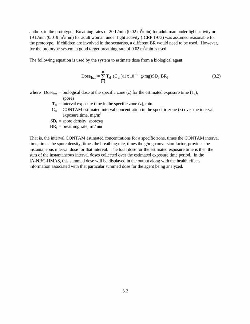
anthrax in the prototype. Breathing rates of 20 L/min (0.02 m3/min) for adult man under light activity or 19 L/min (0.019 m3/min) for adult woman under light activity (ICRP 1973) was assumed reasonable for the prototype. If children are involved in the scenarios, a different BR would need to be used. However, for the prototype system, a good target breathing rate of 0.02 m3/min is used. The following equation is used by the system to estimate dose from a biological agent:

∑=

−=n

1iii

3zizibzt BRSD)mg/g10x1)(C(TDose (3.2)

where Dosebzt = biological dose at the specific zone (z) for the estimated exposure time (Tz), spores Tzi = interval exposure time in the specific zone (z), min Czi = CONTAM estimated interval concentration in the specific zone (z) over the interval exposure time, mg/m3

SDi = spore density, spores/g BRi = breathing rate, m3/min That is, the interval CONTAM estimated concentrations for a specific zone, times the CONTAM interval time, times the spore density, times the breathing rate, times the g/mg conversion factor, provides the instantaneous interval dose for that interval. The total dose for the estimated exposure time is then the sum of the instantaneous interval doses collected over the estimated exposure time period. In the IA-NBC-HMAS, this summed dose will be displayed in the output along with the health effects information associated with that particular summed dose for the agent being analyzed.

4.1

4.0 Health Effect Databases A Biological Health Effect Database (BHED) was developed for evaluating biological agents. The database was developed and populated using anthrax as the example biological agent for the prototype. Likewise a Chemical Health Effects Database (CHED) was developed for evaluating chemical agents. The database was developed and populated using sarin as the example chemical agent for the prototype. The current BHED and CHED are populated only with non-classified information so the prototype system can be demonstrated to a variety of potential clients. In cases where the IA-NBC-HMAS is applied to and tailored to meet specific DOE, DOD, U.S. Department of Justice, and other similar agency assessment needs, the BHED and CHED will likely be populated with classified information on the specific agents of concern. In such cases, the databases and results from an IA-NBC-HMAS run will need to be controlled as classified. Also, the BHED and CHED will need to be populated with health effect information on a variety of biological and chemical agents. It is expected that these databases will grow as the IA-NBC-HMAS is used by clients. The BHED contains the following information fields:

• Agent

• Concentration

• Dose

• Exposure Route

• System of Effect

• Incubation Period

• Contagious Potential

• Acute Health Effects

• Symptoms

• Emergency Medical Action. The CHED contains the following information fields:

• Agent

• Concentration

4.2

• Exposure Time

• Dose

• Acute Health Effect

• Symptoms

• Emergency Medical Action. The data in both databases are all specific to agent concentration levels, so it can be related to specific room or zonal concentration results from the CONTAM model. This allows the health evaluation to be very specific to the different concentration levels resulting from dispersion of the agent throughout the building. Prototype examples of the BHED and CHED are provided in Appendixes C and D, respectively.

5.1

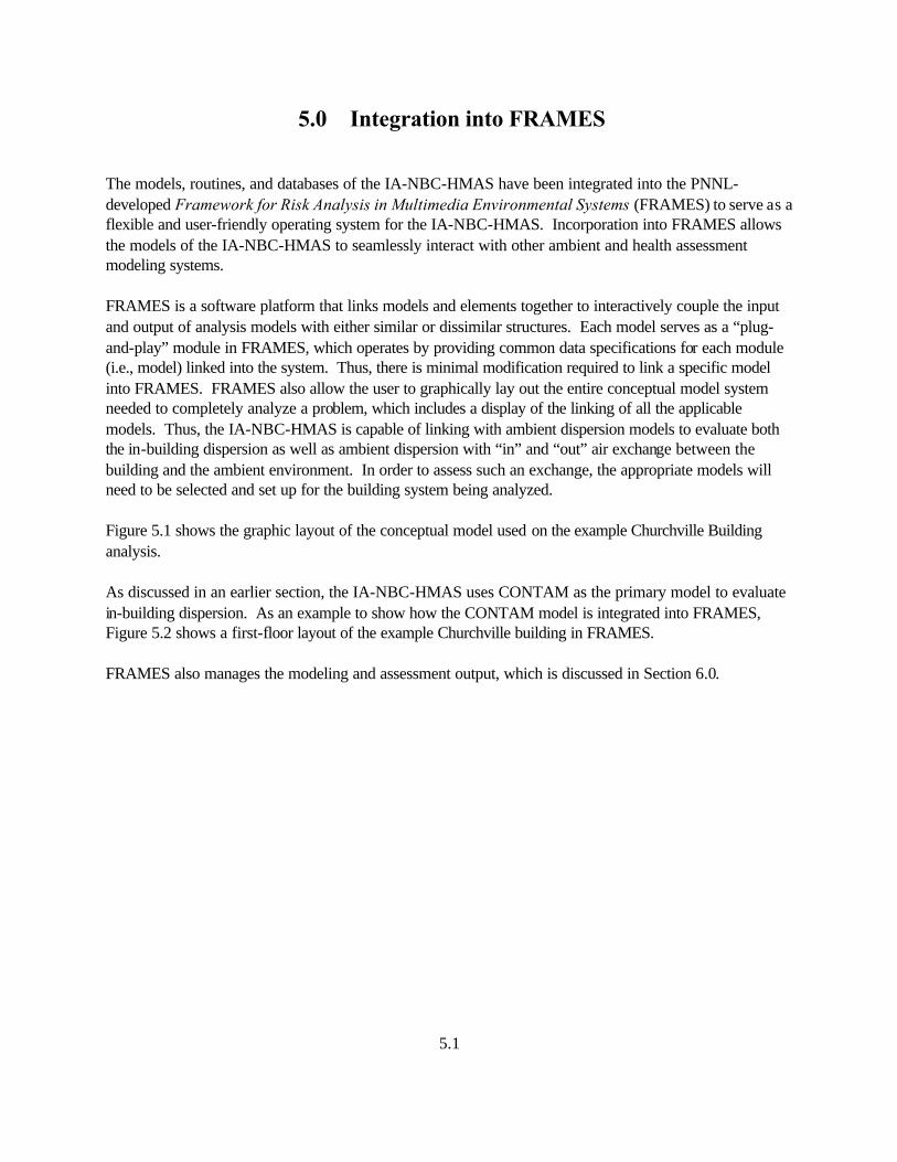
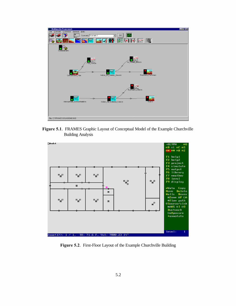
5.0 Integration into FRAMES The models, routines, and databases of the IA-NBC-HMAS have been integrated into the PNNL-developed Framework for Risk Analysis in Multimedia Environmental Systems (FRAMES) to serve as a flexible and user-friendly operating system for the IA-NBC-HMAS. Incorporation into FRAMES allows the models of the IA-NBC-HMAS to seamlessly interact with other ambient and health assessment modeling systems. FRAMES is a software platform that links models and elements together to interactively couple the input and output of analysis models with either similar or dissimilar structures. Each model serves as a “plug-and-play” module in FRAMES, which operates by providing common data specifications for each module (i.e., model) linked into the system. Thus, there is minimal modification required to link a specific model into FRAMES. FRAMES also allow the user to graphically lay out the entire conceptual model system needed to completely analyze a problem, which includes a display of the linking of all the applicable models. Thus, the IA-NBC-HMAS is capable of linking with ambient dispersion models to evaluate both the in-building dispersion as well as ambient dispersion with “in” and “out” air exchange between the building and the ambient environment. In order to assess such an exchange, the appropriate models will need to be selected and set up for the building system being analyzed. Figure 5.1 shows the graphic layout of the conceptual model used on the example Churchville Building analysis. As discussed in an earlier section, the IA-NBC-HMAS uses CONTAM as the primary model to evaluate in-building dispersion. As an example to show how the CONTAM model is integrated into FRAMES, Figure 5.2 shows a first-floor layout of the example Churchville building in FRAMES. FRAMES also manages the modeling and assessment output, which is discussed in Section 6.0.

5.2

Figure 5.1. FRAMES Graphic Layout of Conceptual Model of the Example Churchville Building Analysis

Figure 5.2. First-Floor Layout of the Example Churchville Building

6.1

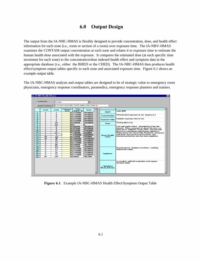
6.0 Output Design The output from the IA-NBC-HMAS is flexibly designed to provide concentration, dose, and health effect information for each zone (i.e., room or section of a room) over exposure time. The IA-NBV-HMAS examines the CONTAM output concentration at each zone and relates it to exposure time to estimate the human health dose associated with the exposure. It compares the estimated dose (at each specific time increment for each zone) to the concentration/dose indexed health effect and symptom data in the appropriate database (i.e., either the BHED or the CHED). The IA-NBC-HMAS then produces health effect/symptom output tables specific to each zone and associated exposure time. Figure 6.1 shows an example output table. The IA-NBC-HMAS analysis and output tables are designed to be of strategic value to emergency room physicians, emergency response coordinators, paramedics, emergency response planners and trainers.

Figure 6.1. Example IA-NBC-HMAS Health Effect/Symptom Output Table

7.1

7.0 Prototype IA-NBC-HMAS Demonstration A demonstration version of the prototype IA-NBC-HMAS is incorporated with this document to allow the reader to examine some of the capabilities of the system. This is a stand-alone demonstration version, in which certain flexible aspects of the CONTAM model and other calculational routines are fixed for simplicity of creating a single file demonstration. As mentioned earlier, the IA-NBC-HMAS operates within the FRAMES systems and potentially couples a variety of models and routines to effect an actual building health assessment. Thus, it is necessary to set up the selected models (i.e., tailor the input parameters) used in an IA-NBC-HMAS analysis to reflect the actual building and environment conditions.

8.1

8.0 References Domestic Preparedness. 50 USC 40, Subchapter 1. International Commission on Radiological Protection (ICRP). 1975. Reference Man: Anatomical Physiological and Metabolic Characteristics. ICRP Publication 23, Pergamon Press, Oxford. McNally, R. E., M. B. Morrison, M. Stark, J. E. Fisher, J. T. Bo'Berry, M. A. Sanzone, and J. E. Berndt. 1993. Effectiveness of Medical Defense Interventions Against Predicted Battlefield Levels of Bacillus Anthacis. F33612-91-D-0652, No. 0002, Science Applications International Corporation, Joppa, Maryland. U.S. Army. 1996. Handbook on the Medical Aspects of NBC Defensive Operations (Part II - Biological and Part III - Chemical). ARMY FIELD MANUAL 8-9 (FM 8-9), NAVMED P-5059, AFJMAN 44-151V1V2V3, U.S. Department of the Army - Office of the Surgeon General, Washington, D.C. U.S. Department of Defense (DOD). 1997. Department of Defense Report to Congress - Domestic Preparedness Program in the Defense Against Weapons of Mass Destruction. U.S. Department of Defense, Washington, D.C. (http://www.defenselink.mil/pubs/domestic/index.html)

Appendix A

Whole-Building Airflow Network Characterization by Inverse Modeling

A.1

Appendix A(a)

Whole-Building Airflow Network Characterization by Inverse Modeling

P. R. Armstrong,(b) P.E., Member

D. L. Hadley,(b) CEM, Member R. D. Stenner,(c) PhD M. C. Janus,(d) P.E., Member

A.1 Abstract Previous efforts to obtain flow-pressure relations and multi-zone network parameters by tracer-gas and other measurements are reviewed. A new method based on simultaneous measurement of all zone pressures within a given control volume and flow measurements on selected inter-zonal paths is presented. Flow rates at a subset of flow measuring locations are controlled during testing to take on two or more values. Constrained, nonlinear least squares analysis produces the power law parameters (flow coefficient and pressure exponent) for each set of two-port aggregate flow paths within the topology. Testing cost and effort are reduced by relying mainly on zone pressure measurements and a rich set of HVAC-induced flow-pressure excitation states with relatively few flow measurements. Results of applying the method to a two-story test building are reported. Application of inverse modeling to fault detection, acceptance testing, continuous commissioning, smoke dispersion and other problems of building performance and operation are outlined.

A.2 Introduction For over 50 years, researchers and weatherization contractors have performed blower door and tracer-gas tests on (mostly detached residential) buildings in order to estimate the energy and IAQ impacts of infiltration and envelope sealing (Dick et al. 1950; Bahnfleth et al. 1957). Similar equipment and procedures have been developed in the last 20 years to estimate duct leakage in the field. Recently, multiply controlled blower-door and multi-tracer-gas test equipment have been marketed to measure leakiness of individual zones and between adjacent zones within a building. On the practical side, test and balance (TAB) technicians routinely make iterative flow measurements at all room air supply points

(a) Paper presented at the ASHRAE 2001 Winter Meeting. For additional information on ASHRAE

publications, contact ASHRAE at www.ashrae.org. (b) Senior Research Engineer, Pacific Northwest National Laboratory, Richland, WA 99352; Armstrong

is currently on educational leave at Massachusetts Institute of Technology. (c) Staff Scientist, Pacific Northwest National Laboratory. (d) Battelle Memorial Institute, Edgewood, MD.

A.2

in newly constructed, renovated, or recommissioned buildings. TAB procedures for tuning distribution and verifying sufficient flow capacity have been with us throughout the history of central heating and cooling. Airflow network(a) modeling became an important research area in the 1980’s. Applications include IAQ and energy modeling, airborne hazard vulnerability assessment & mitigation, and moisture damage research and assessment. Real-time information about building airflows may be extremely useful to new advances in building operation such as continuous commissioning, optimal control, fault detection and diagnosis, and other intelligent building functions. However, a validated, general purpose interzonal model, even in the hands of an experienced user, is not sufficient to ensure accurate predict of air movement in a specific building. Leak parameters input to the model are generally cited as the main source of uncertainty (Sherman 2000), “determining the correct inputs to these models is difficult” (ASHRAE 1997). These assessments are based on the results of field studies that have explored random variations in zone or component leakiness. For example, the normal-ized, log-transformed equivalent leakage area (ELA) distribution in a large sample of apartments of nominally identical construction was found to have a coefficient of variation of over 0.5 (Armstrong et al. 1996); other samples of nominally identical components have turned up correspondingly large variances (Fang and Persily). Many leak sites are inaccessible and it is difficult to isolate the myriad flow paths between zones. The number and aggregate magnitude of these unknown and unintended flow paths is invariably and surprisingly large. “Little information on interzonal leakage has been reported because of the difficulty and expense of measurement” (ASHRAE 1997). Reconciliation of measurements with a corresponding building airflow network model is therefore rarely completed with any degree of analytical rigor, if at all. A practical means of obtaining accurate models of air and contaminant movement in specific buildings with many zones would motivate wider and more effective use of zonal air movement and contaminant dispersion models.

A.3 Background There are several distinct questions that may be posed about air movement in buildings: 1) zone air change rate, 2) interzonal air flow rates, 3) interzonal dispersion of contaminant(s), 4) response of any of the foregoing to wind speed and direction, 5) response of any of the foregoing to a fire. For each of these questions, one can define a forward problem (determining flow rates and zone pressures given system parameters and external pressures) and an inverse problem (determining flow path parameters given measured flow rates, zone pressures, and external pressures). The familiar blower door procedure for determining overall envelope leakiness is, in fact, a simple inverse problem application.

(a) Here we do not address airflows within a zone, which are usually modeled by boundary layer or

computational fluid dynamic models and studied experimentally by flow visualization, interferometry or other special techniques.

A.3

Envelope leakiness is routinely measured in small buildings by blower-door testing (a single-fan pressurization technique) to obtain a power law relation (PLR) between leakage flow rate and indoor-outdoor pressure difference. Multiple fan pressurization techniques are sometimes used to measure inter-zonal air leakage. One such system uses six blower doors operating simultaneously to measure total building envelope leakage area in a 6-unit apartment complex (NEED REF). Modera and Herrlin (1990) refined a two-blower-door tech-nique for measuring the inter-zonal leakage between two adjacent zones in a multi-zone building. A method for measuring airflow rates in HVAC ducts and the building’s airflow system using pulse tracer gas techniques is described by Persily and Axley (1990). It is possible to determine overall leakiness of a building envelope by using the building’s air handling equipment to pressurize the whole building and a constant-injection, tracer gas technique to measure the airflow through the fans (Persily and Grot 1986). The natural pressure differences caused by the stack effect can be used instead of fans to pressurize a building while a tracer technique measures envelope leakage. Opening doors or windows at the top or bottom floors will (de)pressurize the building without using its air handling equipment or external fans (Hayakawa and Togari 1990). These methods all aim to estimate envelope leakiness. They do not provide individual interzonal flow-path parameters needed to model the nonlinear multi-zone airflow network behavior that is characteristic of many single -family houses and most larger buildings. Single-fan measurements with incremental sealing can be used to identify flow parameters for multiple leakage paths. To be reasonably accurate, sealing must be executed in proper sequence (largest to smallest leaks). The method is tedious and often ends with 10-30% of the total ELA unaccounted for. Moreover, the destination (“to-zone”) of leaks identified in one zone (“from-zone”) is often uncertain (Armstrong 1997). Fan pressurization tests characterize envelope leakiness but tell little about air and contaminant movement during normal building operation. A number of methods have been developed for measuring air infil-tration rates in single and multiple zones and rooms. These include constant concentration single tracer gas systems, multi-tracer gas systems using the mass spectrometer, and passive and active perfluoro-carbon multi-tracer systems, capable of measuring average inter-zonal and multi-zonal airflows under changing flow and pressure conditions (Harrje et al. 1990). The simulation of air and contaminant movement is based on well-understood hydrodynamic principles and algorithms. In general, building airflow models fall into two broad categories, multizone models that assume perfect mixing, and single zone, computational fluid dynamic (CFD) models. CFD models usually simulate air movement and contaminant dispersion simultaneously. Zonal models (Walton 1984, Feustel and Dieris 1992) usually solve the air movement problem first and then evaluate contaminant dispersion for a short time step. Transient simulations are executed by repeating the process for many successive time steps. Execution of the multizone forward problem requires specification of a complete air network model. Specification of the zone and airflow path parameters represents the overwhelming bulk of model setup

A.4

work. Parameters describing all envelope leaks, zone volumes, temperatures, and elevations; interzonal leaks; air distribution topology, duct sizes and leak characteristics; damper and fan characteristics must be provided. Musser and Yuill (1999) prepared a very detailed residential building model with 2000 zones and 7000 leakage paths to perform CONTAM(a) simulations of residential infiltration rates. Hiroshi et al. (1999) used COMIS2 to perform an analysis of four kinds of ventilation systems in a residence and used the results to derive a set of predictive equations to evaluate ventilation system performance under any condition. There has been relatively little research (see, e.g., literature review in O’Neill 1989) on the inverse problem, i.e., of identifying a detailed model of a specific building based on its measured response to a range of conditions. In this paper, we develop a method for identifying the parameters for any building that can be modeled as discrete zones connected by airflow paths. The method relies on simultaneous pressure measurement in all zones within a specified control volume and requires relatively few airflow measurements. The zone pressures and (known and unknown) flow rates for a given flow network state describe n mass balance relations, where n is the number of zones. A large number of flow-pressure states can be obtained by varying each of several flow rates independently. A constrained iterative search is used to find the power law relation (PLR) exponents that best (least sum of squared errors) satisfy the mass-balance equations for all states. The PLR coefficients are estimated at each iteration by linear least squares. The governing equations and the solution algorithm are developed and results of numerical experiments are presented.

A.4 Governing Equations A leak path is characterized by a relation between the pressure between its terminating points and the flow through it. Zonal airflow models often characterize leaks by a power law relation defined, for positive flows, by Q = Cpx, where Q is the flow rate, C is a constant, p is the pressure difference between the connected zones, and x is an exponent between 0.5 and 1 (Walton 1997; Walker et al. 1998). What is often considered a single leak is really a complex of flow elements connected in series or parallel or some combination. A window sash, for example, may have different crack widths at the top, bottom, and two sides. The flow-pressure characteristics could be separately measured and the results combined analytically, but it is usual to measure only the aggregate flow and fit a single PLR. Each parallel element can be further decomposed into a set of series elements; for example, there might be two sets of gaskets for the air to pass through. What we accept as being very adequately modeled by a simple two-parameter power law expression is often a complex network of series and parallel paths. A two-port network is a network of any complexity that has only two external terminal nodes. The window sash, as described above, can be considered a two-port network because we can measure and model total leak rate as a function of inside (room node) to outside (ambient node) pressure difference. It

(a) CONTAM and COMIS are widely-used public-domain zonal airflow/IAQ modeling packages

(Feustel).

A.5

is not hard to produce a large number of test cases in CONTAM to demonstrate that the flow-pressure character of most two-port networks of interest in building infiltration problems can be adequately modeled by a single PLR.

A.5 Forward Model Solution Method Zonal flow-pressure models such as CONTAM translate the user-supplied description of a building and its elements into a machine-oriented canonical form. CONTAMX (CONTAM’s solver module) further reduces the description into governing equations that are solved at each time step and integrated over time. CONTAMX represents the system by a pressure-flow relation for each flow path and a mass balance equation for each node. The resulting system of nonlinear equations is solved by the Newton-Raphson (N-R) method. A system of linear equations is constructed by evaluating the partial derivatives of each nonlinear mass-balance equation with respect to each node pressure. A correction vector is evaluated by solving the set of linear equation at each N-R iteration. Upon convergence of zone pressures the flow path equations are evaluated individually to obtain all flow rates. For one section of a 16-story apartment building with about 500 zones and 1000 path elements, the procedure typically converges in about 10 iterations with no wind, and 15 iterations with wind (Armstrong 1996). The pressure drop across each two-port flow element is given by: )zpz(p g )P (P p 221121 −+= (A.1) where p = pressure drop across flow element of interest P1, P2 = pressure at base of from-zone and to-zone ρ = air density g = acceleration of gravity (9.81 m/s2) z1, z2 = entry and exit elevations with respect to base of from-zone and to-zone. Walton (1997) describes three variants of the empirical PLR flow-pressure relation: Volumetric flow rate Q = Cpn Mass flow rate F = Cpn Root-density-corrected flow rate Q = (ño/ñ)½Cpn where ρo = reference density The flow network can be completely described by a list of zones, each described by base elevation and air density, and a list of two-port paths, each described by C, x, from- and to-zone pointers, and from- and to-zone elevations (z1 and z2). A mass balance for the ith zone is given by Ój�i(Fij) = ri where Fij denotes flow from the jth zone to the ith zone and Ój�i denotes summation over all from-zones. Network airflows and pressures for given boundary conditions (fixed pressures and flow rates) are solved by applying Newton-Raphson iteration to the n mass flow equations until all residuals, ri, i=1:n, are forced to zero. Additional details of how N-R is efficiently applied to this special type of problem are outlined in Attachment A.

A.6

A.6 Inverse Model Formulation The forward problem just described may be summarized thus. We have n unknown pressures, and n node equations to be solved for a given set of boundary conditions (fan settings, buoyant forces, and wind pressures). The system of equations comprises a set of linked mass balance equations which can be solved tediously by successive relaxation (Cross 1934) or very efficiently by the Newton-Raphson (N-R) procedure (Martin and Peters 1963; Walton 1984). The inverse problem (with all flow elements modeled by PLRs) has 2m unknowns, where m is the number of two-port paths and, typically, m>>n. The system will still consist of a set of linked mass balance equations, but the n-vector of pressures measured at one network flow state will not provide enough information to solve the 2m unknowns. By exciting the system in different ways, one may effectively produce replicates of the mass balance equations with different boundary conditions. Moreover, by exciting the system in many different ways, one compensates, to large extent, for random measurement error. That is, a richly varying set of boundary conditions reduces the minimum number of flow and pressure measuring stations required. Mass Balance Equations . The inverse problem departs from the forward problem, (wherein the pressures are unknown) in its use of pressure differences instead of zone pressures. The first step in the analysis is to convert zone pressures to flow element pressure differences after which the zone pressures are never again referenced. In the balance of this paper the phrase “flow element pressure” will be understood to mean “signed pressure difference across a given two-port flow element.” The mass balance for zone i is expressed very generally in terms of all flow element pressures, pj, as follows:

∑ ∑= =

β=δm

1j

m

1jjj,i

xjjj,i FpC j (A.2)

where m is the number of two-port paths in the system Cj, xj are the unknown parameters of the jth flow element Fj is the measured flow in the jth flow element âi,j = (-1, 0, 1) is the sign of the measured flow j into zone i äi,j = (-1, 0, 1) is the sign of the unmeasured flow j into zone i. The parameters, â and ä, establish the topology of the system. Nonzero values of ä are assigned only to those paths, j, connected to a given zone, i. The usual sign convention is positive for a flow into the ith zone.

A.7

Every fan-induced flow must be measured(a) and assigned to the appropriate right-hand side (RHS) sum. It is theoretically possible to obtain a useful solution with just one of the equations having a non-zero value on the RHS, provided sufficient accuracy and richness of variation in pressure (wind, temperature, and fan-induced) boundary conditions. However, we expect that in practice the number of measured flows (corresponding to non-zero RHS terms) will have to be a substantial fraction of the number of zones. Note that for any passive measured flow, j, (e.g., at a return air grille flow station) the flow element parameters (Cj,xj) are estimated by the usual blower-door flow-pressure regression independent of the flow-pressure network problem. The corresponding äi,j’s used in the inverse network problem must be set to zero. Topology. The topology matrices, [âi,k] and [äi,k], may be conveniently generated by preparing a CONTAM model of the building of interest. Multiple paths between a given pair of CONTAM zones must be aggregated into a single two-port path. Only zones with measured pressures can be admitted to the model. The CONTAM model (.ndf file) will list m paths. Each measured flow is represented by a constant mass flow rate (fan) element or by a supply or return register associated with a simple (b) air handler. A program has been written to produce the topology matrices, [âi,j] and [äi,j], by reading the CONTAM generated project description file corresponding to the user’s building description(c). A second program was written to produce “data” for initial testing of the inverse modeling analysis. The latter program generates a large number of unique flow excitation states and calls CONTAMX(d) to solve the flow-pressure network at each state. A mix of fan and supply register flow elements may be used to excite the system. The air source/sink for a fan may be zone 0 (outside ambient) or the fan may induce airflow between any pair of (usually adjacent) zones. A flow element representing the aggregate of unmeasured passive flows between adjacent zones may also be included in the model as a separate flow-pressure relation with unknown parameters. This situation is reflected in the topology vectors when ä contains a non-zero element corresponding to a non-zero element of â, i.e., |äi,j | = |âi,j | = 1 for a particular i and j. The training data set contains (sum over topologies, t) Óntst data “points” where nt is the number of zones and st is the number of system excitation states for a given flow measuring topology, t. The simple problems presented in this paper use only one topology, t=1, but flow and pressure monitoring equipment limits may necessitate that a large, complex building be subdivided into isolated or overlapping control volumes each representing a portion of the overall airflow network.

(a) By measuring fan power, speed and pressure with suitable precision, it is possible to infer flow rate by means of a carefully formulated and calibrated fan curve. (b) CONTAM’s “simple air handler” model provides a specified constant flow rate at each register. (c) A baseline topology may be supplemented by one or more alternate test topologies in which selected measured flow elements are added or inserted in place of existing passive flow paths. Some of these topologies may involve only a subset of zones. (d) CONTAMX (public domain) is the solver portion of CONTAM and is command-line callable.

A.8

A.7 Inverse Model Solution Method If the exponent of each power law relation is specified, the over-determined system of equations is linear and can be readily solved by linear least squares. Some flow network problems are but moderately sensitive to the exponent estimates. For example, one can assign an exponent of 0.5 to cracks and other openings wider than 2mm, 0.7 to small cracks, and 0.8 to porous flow elements. The power law coefficients determined by least squares will be quite sensitive to the exponent estimates but the ELAs much less so. One test of this approach—described later in the paper (Test 3)—resulted in root-mean-square (rms) deviation of less than 1% of true flow and maximum deviation of less than 2% of true flow. In cases where it is important that the exponents, as well as the power law coefficients, be determined from field data, the least squares model fitting criterion is still appropriate but the ordinary least squares algorithm is not directly applicable. A hybrid search algorithm has been developed for this purpose. In this hybrid scheme, power law exponents are determined by a constrained, iterative (steepest descent or conjugate gradient) search algorithm. Computational efficiency must be considered when the iterative search is applied to a network with a large number, m, of flow paths. Appropriate sparse matrix methods (Walton 1997) may be beneficially applied to the linear system involving the power law coefficients that must be solved at each iteration. Computational effort is on the order of m3 for the standard least squares problem. Note that the sparse matrix pattern is defined by the LHS topology matrix, [L]. Various optimization methods are available to solve nonlinear least squares problems (Brent 1973, Gill et al. 1981, Press 1992). Most of the results reported in this paper have been obtained by the simple constrained steepest descent algorithm presented in Attachment B and summarized below. The search begins with an initial estimate of x, the vector of all power law exponents. Linear regression is applied to determine the mean-squared mass flow balance error as the exponents are perturbed one by one; the resulting gradient vector, u, defines the steepest descent direction in power law exponent space. Linear regression is performed at points along this line to find the distance, d, to the minimum (mean squared error) point. However, d must be constrained by limiting R = ||r|| such that the feasible region 0.5 � riui � 1.0, within x-space is not violated. Finally, the new base point for the next high-level iteration is evaluated: udsx += One important adjustment can be made at this point to reduce the number of trial distances in successive iterations. If d is much smaller than R, R should be reduced. If, on the other hand, the line search ends at d=R, R should be increased if this can be done without violating an exponent constraint.

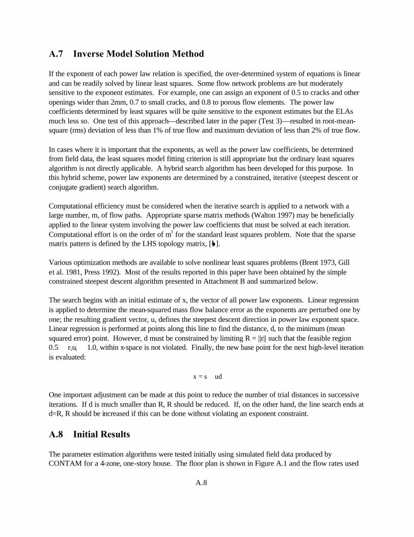
A.8 Initial Results The parameter estimation algorithms were tested initially using simulated field data produced by CONTAM for a 4-zone, one-story house. The floor plan is shown in Figure A.1 and the flow rates used

A.9

12

7

14

2

6

119

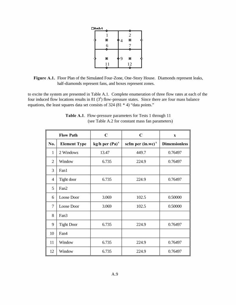
Figure A.1. Floor Plan of the Simulated Four-Zone, One-Story House. Diamonds represent leaks, half-diamonds represent fans, and boxes represent zones. to excite the system are presented in Table A.1. Complete enumeration of three flow rates at each of the four induced flow locations results in 81 (34) flow-pressure states. Since there are four mass balance equations, the least squares data set consists of 324 (81 * 4) “data points.”

Table A.1. Flow-pressure parameters for Tests 1 through 11 (see Table A.2 for constant mass fan parameters)

Flow Path C C x

No. Element Type kg/h per (Pa)x scfm per (in.wc) x Dimensionless

1 2 Windows 13.47 449.7 0.76497

2 Window 6.735 224.9 0.76497

3 Fan1

4 Tight door 6.735 224.9 0.76497

5 Fan2

6 Loose Door 3.069 102.5 0.50000

7 Loose Door 3.069 102.5 0.50000

8 Fan3

9 Tight Door 6.735 224.9 0.76497

10 Fan4

11 Window 6.735 224.9 0.76497

12 Window 6.735 224.9 0.76497

A.10

Table A.2. Excitation Grid Mass Flow Rates for Tests 1 Through 7

Flow Path

No. Element

Excitation Flow Rates (kg/h)

Excitation Flow Rates (scfm)

3 Fan1 204.6 61.4 20.5 100 30 10

5 Fan2 204.6 61.4 20.5 100 30 10

8 Fan3 204.6 61.4 20.5 100 30 10

10 Fan4 204.6 61.4 20.5 100 30 10

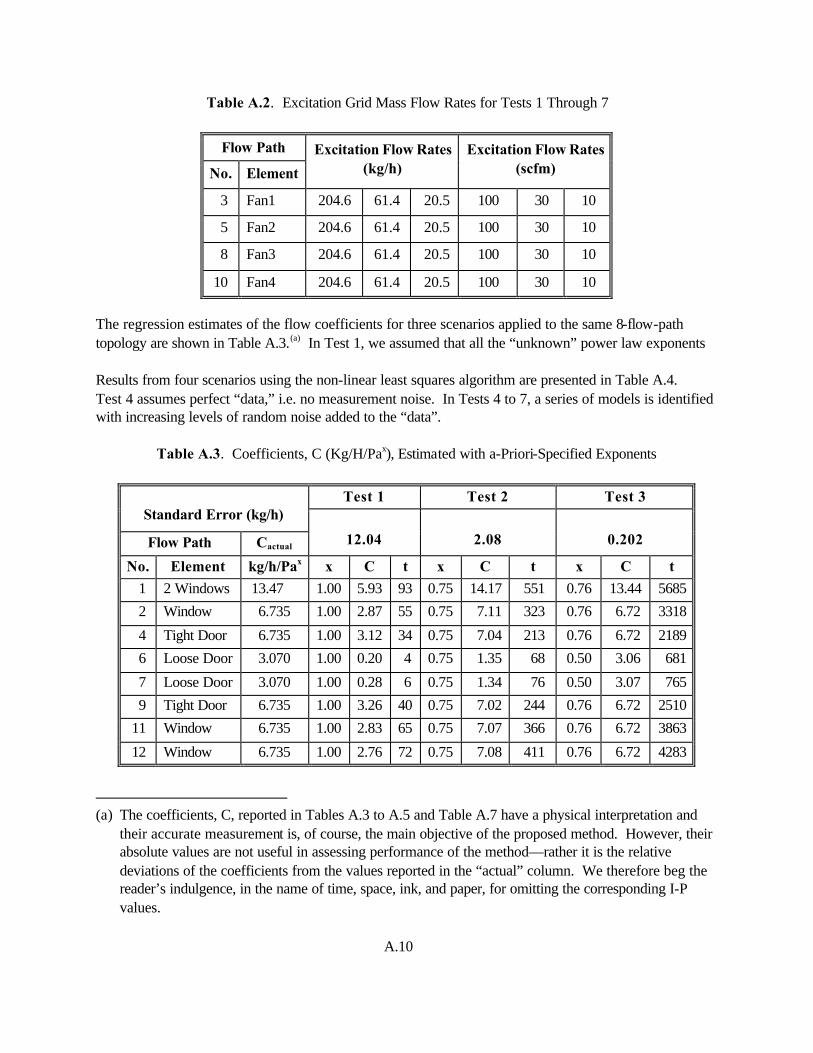
The regression estimates of the flow coefficients for three scenarios applied to the same 8-flow-path topology are shown in Table A.3.(a) In Test 1, we assumed that all the “unknown” power law exponents Results from four scenarios using the non-linear least squares algorithm are presented in Table A.4. Test 4 assumes perfect “data,” i.e. no measurement noise. In Tests 4 to 7, a series of models is identified with increasing levels of random noise added to the “data”.

Table A.3. Coefficients, C (Kg/H/Pax), Estimated with a-Priori-Specified Exponents

Test 1 Test 2 Test 3 Standard Error (kg/h)

Flow Path Cactual 12.04 2.08 0.202

No. Element kg/h/Pax x C t x C t x C t

1 2 Windows 13.47 1.00 5.93 93 0.75 14.17 551 0.76 13.44 5685

2 Window 6.735 1.00 2.87 55 0.75 7.11 323 0.76 6.72 3318

4 Tight Door 6.735 1.00 3.12 34 0.75 7.04 213 0.76 6.72 2189

6 Loose Door 3.070 1.00 0.20 4 0.75 1.35 68 0.50 3.06 681

7 Loose Door 3.070 1.00 0.28 6 0.75 1.34 76 0.50 3.07 765

9 Tight Door 6.735 1.00 3.26 40 0.75 7.02 244 0.76 6.72 2510

11 Window 6.735 1.00 2.83 65 0.75 7.07 366 0.76 6.72 3863

12 Window 6.735 1.00 2.76 72 0.75 7.08 411 0.76 6.72 4283

(a) The coefficients, C, reported in Tables A.3 to A.5 and Table A.7 have a physical interpretation and

their accurate measurement is, of course, the main objective of the proposed method. However, their absolute values are not useful in assessing performance of the method—rather it is the relative deviations of the coefficients from the values reported in the “actual” column. We therefore beg the reader’s indulgence, in the name of time, space, ink, and paper, for omitting the corresponding I-P values.

A.11

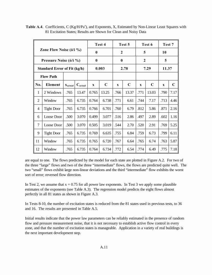
Table A.4. Coefficients, C (Kg/H/Pax), and Exponents, X, Estimated by Non-Linear Least Squares with 81 Excitation States; Results are Shown for Clean and Noisy Data

Test 4 Test 5 Test 6 Test 7 Zone Flow Noise (ó/ì %)

0 2 5 10

Pressure Noise (ó/ì %) 0 0 2 5

Standard Error of Fit (kg/h) 0.003 2.78 7.29 11.37

Flow Path

No. Element xactual Cactual x C x C x C x C

1 2 Windows .765 13.47 0.765 13.25 .766 13.37 .771 13.03 .790 7.17

2 Window .765 6.735 0.764 6.738 .771 6.61 .744 7.17 .713 4.46

4 Tight Door .765 6.735 0.766 6.701 .760 6.79 .812 5.86 .871 2.16

6 Loose Door .500 3.070 0.499 3.077 .516 2.86 .497 2.89 .602 1.16

7 Loose Door .500 3.070 0.505 3.019 .544 2.70 .520 2.91 .769 5.25

9 Tight Door .765 6.735 0.769 6.635 .755 6.84 .759 6.73 .799 6.11

11 Window .765 6.735 0.765 6.720 .767 6.64 .765 6.74 .763 5.87

12 Window .765 6.735 0.764 6.734 .772 6.54 .774 6.49 .775 7.18

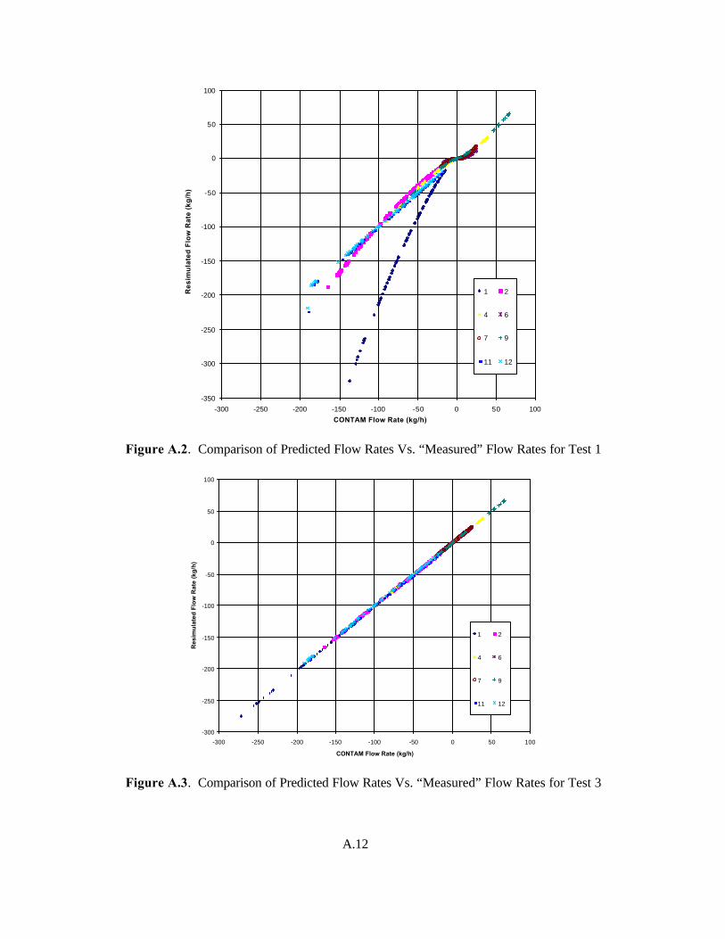
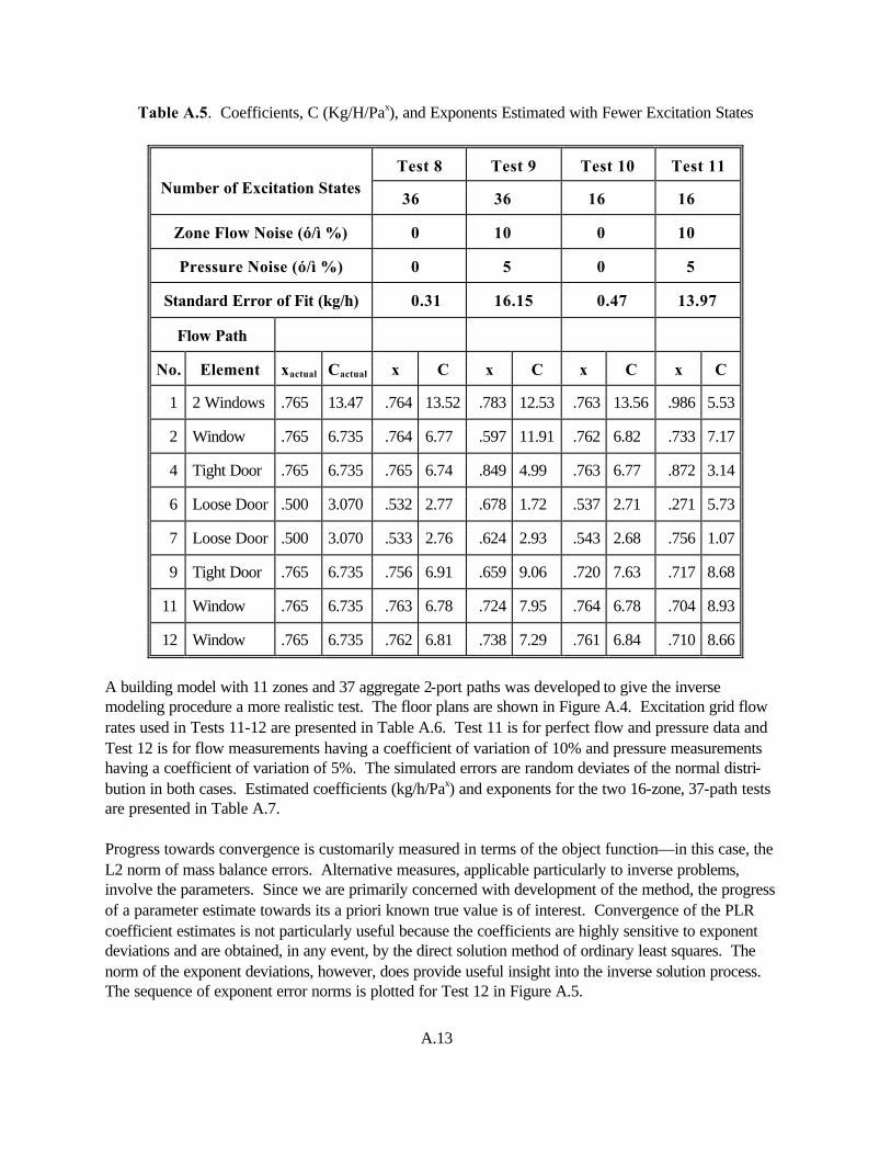
are equal to one. The flows predicted by the model for each state are plotted in Figure A.2. For two of the three “large” flows and two of the three “intermediate” flows, the flows are predicted quite well. The two “small” flows exhibit large non-linear deviations and the third “intermediate” flow exhibits the worst sort of error; reversed flow direction. In Test 2, we assume that x = 0.75 for all power law exponents. In Test 3 we apply some plausible estimates of the exponents (see Table A.3). The regression model predicts the eight flows almost perfectly in all 81 states as shown in Figure A.3. In Tests 8-10, the number of excitation states is reduced from the 81 states used in previous tests, to 36 and 16. The results are presented in Table A.5. Initial results indicate that the power law parameters can be reliably estimated in the presence of random flow and pressure measurement noise, that it is not necessary to establish active flow control in every zone, and that the number of excitation states is manageable. Application in a variety of real buildings is the next important development step.

A.12

-350

-300

-250

-200

-150

-100

-50

0

50

100

-300 -250 -200 -150 -100 -50 0 50 100

CONTAM Flow Rate (kg/h)

Res

imu

late

d F

low

Rat

e (k

g/h

)

1 2

4 6

7 9

11 12

Figure A.2. Comparison of Predicted Flow Rates Vs. “Measured” Flow Rates for Test 1

-300

-250

-200

-150

-100

-50

0

50

100

-300 -250 -200 -150 -100 -50 0 50 100

CONTAM Flow Rate (kg/h)

Res

imul

ated

Flo

w R

ate

(kg/

h)

1 2

4 6

7 9

11 12

Figure A.3. Comparison of Predicted Flow Rates Vs. “Measured” Flow Rates for Test 3

A.13

Table A.5. Coefficients, C (Kg/H/Pax), and Exponents Estimated with Fewer Excitation States

Test 8 Test 9 Test 10 Test 11 Number of Excitation States

36 36 16 16

Zone Flow Noise (ó/ì %) 0 10 0 10

Pressure Noise (ó/ì %) 0 5 0 5

Standard Error of Fit (kg/h) 0.31 16.15 0.47 13.97

Flow Path

No. Element xactual Cactual x C x C x C x C

1 2 Windows .765 13.47 .764 13.52 .783 12.53 .763 13.56 .986 5.53

2 Window .765 6.735 .764 6.77 .597 11.91 .762 6.82 .733 7.17

4 Tight Door .765 6.735 .765 6.74 .849 4.99 .763 6.77 .872 3.14

6 Loose Door .500 3.070 .532 2.77 .678 1.72 .537 2.71 .271 5.73

7 Loose Door .500 3.070 .533 2.76 .624 2.93 .543 2.68 .756 1.07

9 Tight Door .765 6.735 .756 6.91 .659 9.06 .720 7.63 .717 8.68

11 Window .765 6.735 .763 6.78 .724 7.95 .764 6.78 .704 8.93

12 Window .765 6.735 .762 6.81 .738 7.29 .761 6.84 .710 8.66

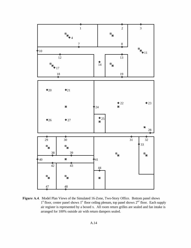
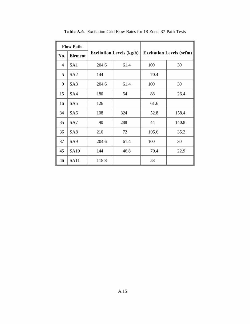
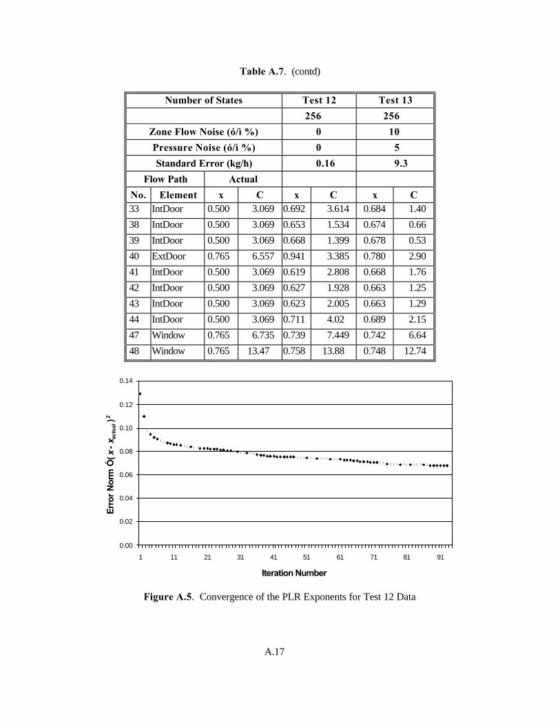
A building model with 11 zones and 37 aggregate 2-port paths was developed to give the inverse modeling procedure a more realistic test. The floor plans are shown in Figure A.4. Excitation grid flow rates used in Tests 11-12 are presented in Table A.6. Test 11 is for perfect flow and pressure data and Test 12 is for flow measurements having a coefficient of variation of 10% and pressure measurements having a coefficient of variation of 5%. The simulated errors are random deviates of the normal distri-bution in both cases. Estimated coefficients (kg/h/Pax) and exponents for the two 16-zone, 37-path tests are presented in Table A.7. Progress towards convergence is customarily measured in terms of the object function—in this case, the L2 norm of mass balance errors. Alternative measures, applicable particularly to inverse problems, involve the parameters. Since we are primarily concerned with development of the method, the progress of a parameter estimate towards its a priori known true value is of interest. Convergence of the PLR coefficient estimates is not particularly useful because the coefficients are highly sensitive to exponent deviations and are obtained, in any event, by the direct solution method of ordinary least squares. The norm of the exponent deviations, however, does provide useful insight into the inverse solution process. The sequence of exponent error norms is plotted for Test 12 in Figure A.5.

A.14

1 2

8

13

7

19

12

11

17

4

10

27

3

24

28

14

26

20 21

22

29

23

25

32 31

38

30

40

33

42 44

39

47

43

41

48

18

Figure A.4. Model Plan Views of the Simulated 16-Zone, Two-Story Office. Bottom panel shows 1st floor, center panel shows 1st floor ceiling plenum, top panel shows 2nd floor. Each supply air register is represented by a boxed x. All room return grilles are sealed and fan intake is arranged for 100% outside air with return dampers sealed.

A.15

Table A.6. Excitation Grid Flow Rates for 18-Zone, 37-Path Tests

Flow Path

No. Element Excitation Levels (kg/h) Excitation Levels (scfm)

4 SA1 204.6 61.4 100 30

5 SA2 144 70.4

9 SA3 204.6 61.4 100 30

15 SA4 180 54 88 26.4

16 SA5 126 61.6

34 SA6 108 324 52.8 158.4

35 SA7 90 288 44 140.8

36 SA8 216 72 105.6 35.2

37 SA9 204.6 61.4 100 30

45 SA10 144 46.8 70.4 22.9

46 SA11 118.8 58

A.16

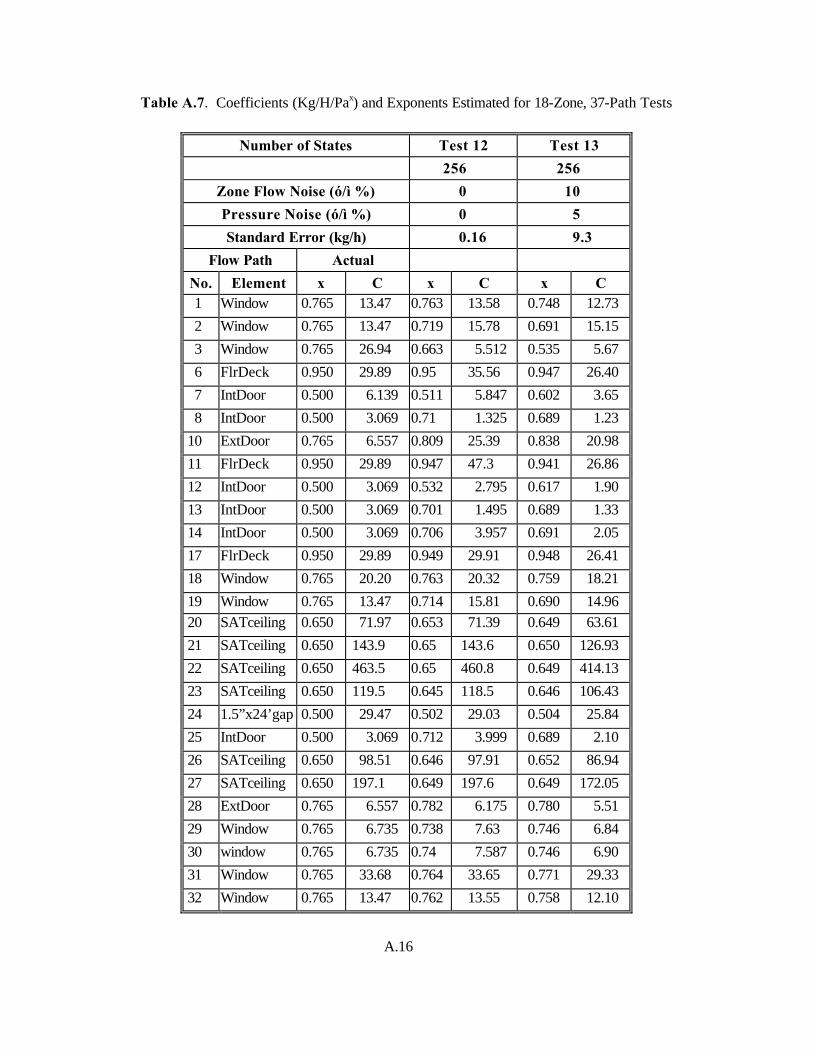
Table A.7. Coefficients (Kg/H/Pax) and Exponents Estimated for 18-Zone, 37-Path Tests

Number of States Test 12 Test 13

256 256

Zone Flow Noise (ó/ì %) 0 10

Pressure Noise (ó/ì %) 0 5

Standard Error (kg/h) 0.16 9.3

Flow Path Actual

No. Element x C x C x C 1 Window 0.765 13.47 0.763 13.58 0.748 12.73

2 Window 0.765 13.47 0.719 15.78 0.691 15.15

3 Window 0.765 26.94 0.663 5.512 0.535 5.67

6 FlrDeck 0.950 29.89 0.95 35.56 0.947 26.40

7 IntDoor 0.500 6.139 0.511 5.847 0.602 3.65

8 IntDoor 0.500 3.069 0.71 1.325 0.689 1.23

10 ExtDoor 0.765 6.557 0.809 25.39 0.838 20.98

11 FlrDeck 0.950 29.89 0.947 47.3 0.941 26.86

12 IntDoor 0.500 3.069 0.532 2.795 0.617 1.90

13 IntDoor 0.500 3.069 0.701 1.495 0.689 1.33

14 IntDoor 0.500 3.069 0.706 3.957 0.691 2.05

17 FlrDeck 0.950 29.89 0.949 29.91 0.948 26.41

18 Window 0.765 20.20 0.763 20.32 0.759 18.21

19 Window 0.765 13.47 0.714 15.81 0.690 14.96 20 SATceiling 0.650 71.97 0.653 71.39 0.649 63.61

21 SATceiling 0.650 143.9 0.65 143.6 0.650 126.93

22 SATceiling 0.650 463.5 0.65 460.8 0.649 414.13

23 SATceiling 0.650 119.5 0.645 118.5 0.646 106.43

24 1.5”x24’gap 0.500 29.47 0.502 29.03 0.504 25.84

25 IntDoor 0.500 3.069 0.712 3.999 0.689 2.10

26 SATceiling 0.650 98.51 0.646 97.91 0.652 86.94

27 SATceiling 0.650 197.1 0.649 197.6 0.649 172.05

28 ExtDoor 0.765 6.557 0.782 6.175 0.780 5.51

29 Window 0.765 6.735 0.738 7.63 0.746 6.84

30 window 0.765 6.735 0.74 7.587 0.746 6.90

31 Window 0.765 33.68 0.764 33.65 0.771 29.33

32 Window 0.765 13.47 0.762 13.55 0.758 12.10

A.17

Table A.7. (contd)

Number of States Test 12 Test 13

256 256

Zone Flow Noise (ó/ì %) 0 10

Pressure Noise (ó/ì %) 0 5

Standard Error (kg/h) 0.16 9.3

Flow Path Actual

No. Element x C x C x C 33 IntDoor 0.500 3.069 0.692 3.614 0.684 1.40

38 IntDoor 0.500 3.069 0.653 1.534 0.674 0.66

39 IntDoor 0.500 3.069 0.668 1.399 0.678 0.53

40 ExtDoor 0.765 6.557 0.941 3.385 0.780 2.90

41 IntDoor 0.500 3.069 0.619 2.808 0.668 1.76

42 IntDoor 0.500 3.069 0.627 1.928 0.663 1.25

43 IntDoor 0.500 3.069 0.623 2.005 0.663 1.29

44 IntDoor 0.500 3.069 0.711 4.02 0.689 2.15

47 Window 0.765 6.735 0.739 7.449 0.742 6.64

48 Window 0.765 13.47 0.758 13.88 0.748 12.74

0.00

0.02

0.04

0.06

0.08

0.10

0.12

0.14

1 11 21 31 41 51 61 71 81 91

Iteration Number

Err

or N

orm

Ó(x

- xac

tual

)2

Figure A.5. Convergence of the PLR Exponents for Test 12 Data

A.18

A.9 Implementation Flows into selected zones and between selected zone pairs can be induced by traditional blower door equipment or by adapting the existing air distribution system to the purpose. If the distribution system is used, duct leakage must be thoroughly characterized and duct pressure measured during zone pressure tests so that leakage flow rates can be evaluated for each flow excitation state. This characterization is needed to model the flow-pressure network during fan operation in any event. Accurate quasi-simultaneous measurement of a large number of pressures, while less a challenge than measuring a similar number of airflows, will be costly. A pneumatic multiplexing scheme (borrowed from wind tunnel research practice) can be used to reduce monitoring costs. Temperature-density corrections must be applied to sampling tubes with vertical runs. Continuing progress in cost-performance value of off-the-shelf sensitive, stable pressure transducers is also helping the situation. In general, it is desirable to measure pressures in all zones with respect to ambient on a calm day while varying the supply airflow rate to each zone. Returns can be fully blocked or can, in many cases, be used as additional flow measurement and regulation stations. Blower doors are still a practical necessity in buildings that lack mechanical air distribution systems and may be used to supplement the manipulation of supply or return airflows as well. Field experience with the new method is needed to determine if it is possible to test on windy days by obtaining simultaneous wind pressure measurements. Guidance on the spatial resolution of wind pressure taps will also be needed.

A.10 Discussion We believe that experience will demonstrate the importance of interactive flow network modeling to rapid acquisition of a network’s main flow path characteristics and to the resolution of problem zones and flow paths. These problem flow elements typically need testing over wide flow or pressure ranges or require greater concentration of local flow and pressure measurement points in a particular subset of zones, duct networks, and chase, plenum or framing cavities. The expense of making such measurements exhaus-tively throughout an entire building would rarely be justified. But with interactive analysis of building airflows and pressures, the few areas where such detailed measurements are really needed can be quickly identified in the field. Additional detailed measurements become very cost effective when it takes only a few such measurements to reward the analyst with a significant reduction in uncertainty (Armstrong 1997). In Tests 1-12 we have treated the residual of each mass balance equation with equal weight. There is some indication that the ratio of residual to total zone flow may give “better” results. Adapting the embedded least-squares routine to compute weighted least-squares power law coefficients presents no great difficulty. The benefits and details of this approach, however, will have to be assessed with extensive field data. The sensitivity of results to errors in the independent variables (pressure differences—which must be error free to be sure of obtaining the good statistical properties customarily attributed to ordinary least squares) should also be assessed and possibly addressed by modification of the least squares analysis.

A.19

Physical reasoning leads us to expect problems when the maximum (under a range of excitations) flow magnitude on a given path is a small fraction of the greater of the two mass air change rates in its associated zones. A software package could re-simulate test conditions and report the path-to-zone flow ratios by magnitude to guide the field engineer in devising additional tests and test conditions. The value of using such re-simulation results, vis-à-vis reliance on t-ratios alone to guide supplemental testing, needs to be explored. Analysis of large, complex networks will tax computing resources in terms of both memory and execution time. Such networks can be decomposed into arbitrarily small sub networks with known boundary conditions. However, problems can be expected when the sample sizes are effectively reduced in pursuing this simplifying measure. Least-squares parameter estimation can be expected to return the best results when applied to control volumes with many zones, measured flow rates, and excitation states.

A.11 Conclusion Zonal modeling has many important applications such as air distribution and ventilation design, estima-tion of energy use, analysis of smoke management and contaminant dispersion, and other IAQ modeling activities. Leak parameters input to a zonal model are frequently cited as the greatest source of uncer-tainty in predicting flow and air change rates. Leak characterization by traditional blower-door methods is difficult and intrusive and leak parameters are not easily derived from tracer data. The number and aggregate magnitude of unknown and unintended flow paths is invariably and surprisingly large. Acquisition of complete leakiness data and reconciliation of measurements with a corresponding building airflow network model has therefore rarely been attempted. To address these problems, a new method, based on simultaneous measurement of pressures in all zones and flow measurements on selected paths, has been developed. A constrained, nonlinear least squares analysis is used to obtain power law parameters (flow coefficient and exponent) for each two-port aggregate flow path defined in the topology. The governing equations and an efficient parameter estimation algorithm have been presented. Numerical “experiments” with the algorithm give very positive results. The inverse modeling method and associated test protocol maximize the ratio of interzonal leak parameters acquired to flow stations deployed by relying mainly on zone pressure measurements and a rich set of flow-pressure excitation states. Cost and effort are reduced because pressure measurement is less costly and intrusive than flow measurement.

A.12 Nomenclature Ci coefficient of the power law flow-pressure relation for ith flow element d distance (from previous search point) along current line of steepest descent Fi measured flow associated with the ith zone, J(x) value of the objective function evaluated at x = [xi] pi signed pressure difference across ith flow element, Pi absolute pressure at the floor of zone i,

A.20

R maximum distance to search on the current line of steepest descent ri positive distance beyond which the ith constraint is violated ui i

th element of the steepest descent unit direction vector, u xi exponent of the power law flow-pressure relation for a two-port flow element âi 0 (-1, 0, 1) ith entry in the topology vector mapping measured flows to zones äi 0 (-1, 0, 1) ith entry in the topology vector mapping unmeasured flows to zones.

A.13 References Armstrong, P. R., J. A. Dirks, Y. Matrosov, J. Olkinaru, D. Saum. 1996. Infiltration and Ventilation in Russian Multi-Family Buildings. ACEEE Summer Study on Energy Efficiency in Buildings. Armstrong, P. R., B. Y. Nekrasov, I. Sultanguzin. 1997. Infiltration Leak Characterization by Blower Door Tests. Report to the Foundation for Enterprise Restructuring and Financial Institutions Development, Moscow. ASHRAE. 1997. 1997 ASHRAE Handbook—Fundamentals, Chapter 25: Ventilation and Infiltration, Atlanta: American Society of Heating, Refrigerating, and Air-Conditioning Engineers, Inc. Bahnfleth, D. R., T. D. Moseley and W. S. Harris. 1957. Measurement of infiltration in two residences. ASHRAE Transactions 63(2):439-452. Brent, R. P. 1973. Algorithms for Minimization without Derivatives. Englewood Cliffs: Prentice-Hall. Cross, H. 1934. Analysis of Flow in Networks of Conduits and Connectors. Bulletin #286, U. Illinois, Engineering Experiment Station. Dick, J. B., Garston, Watford, Herts. 1950. Measurement of ventilation using tracer gas technique. J. HPAC, May. Feustel, H. E. and J. Dieris. 1992. A survey of airflow models for multizone structures. Energy and Buildings, Vol. 18, pp. 79-100. Gill, P. E., W. Murray, and M. H. White. 1981. Practical Optimization. New York: Academic Press. Harrje, D. T., R. N. Dietz, M. H. Sherman, D. L. Bohac, T. W. D’Ottavio and D. J. Dickerhoff. 1990. Tracer Gas Measurement Systems Compared in Multifamily Building. Air Change Rate and Airtightness in Buildings, ASTM STP 1067, M. H. Sherman, Ed. Philadelphia: American Society for Testing and Materials, pp. 5-20. Hayakawa, S. and S. Togari. 1990. Simplified Test Method for Evaluating Exterior Wall Airtightness of Tall Office Buildings. Air Change Rate and Airtightness in Buildings, ASTM STP 1067, M. H. Sherman, Ed. Philadelphia: American Society for Testing and Materials.

A.21

Hiroshi, Y., J. Liu, H. E. Feustel, J-R. Millet, L-G. Mansson. 1999. Numerical analysis of ventilation system performance by the COMIS model. ASHRAE Transactions 105(2). Martin, D. W. and G. Peters. 1963. The application of Newton’s method to network analysis by digital computer. (UK) Journal of the Institute of Water Engineers, V. 17. Modera, M. P. and M. K. Herrlin. 1990. Investigation of a Fan-Pressurization Technique for Measuring Interzonal Air Leakage. ASTM STP 1067, M. H. Sherman, Editor. Philadelphia: American Society for Testing and Materials, pp. 183-192. Musser, A. and G. K. Yuill. 1999. Comparison of residential air infiltration rates predicted by single -zone and multizone models. ASHRAE Transactions 105(2). O’Neill, P.J. and R.R. Crawford. 1989. Multi-zone flow analysis and zone selection using a new pulsed tracer gas technique. Espoo: Proc 10th AIVC Conference. Persily, A. and J. Axley. 1990. Measuring Airflow Rates with Pulse Tracer Techniques. Air Change Rate and Airtightness in Buildings, ASTM STP 1067, M.H. Sherman, Ed., American Society for Testing and Materials, Philadelphia, pp. 31-51. Persily, A.K. and R.A. Grot. 1986. Pressurization Testing of Federal Buildings. Measured Air Leakage of Buildings, ASTM STP 904, H.R. Trechsel and P.L. Lagus, Eds., American Society for Testing and Materials, Philadelphia, pp. 184-200. Press, William H., 1992. Numerical Recipes in FORTRAN : The Art of Scientific Computing, 2nd Edition, Cambridge University Press. Sherman, M.H. and D. Jump. 2000. Energy conservation in buildings, Chapter 6.3 of Handbook of Heating Ventilation and Air Conditioning, Jan Kreider, ed., CRC Press. Walker, I.S., D.J. Wilson and M.H. Sherman.1998. A comparison of the power law to quadratic formulations for air infiltration calculations. Energy and Buildings 27:293-299 Walton, G.N. 1984. A computer algorithm for predicting infiltration and inter-zone airflows. ASHRAE Transactions 90(1). Walton, G.N. 1997. CONTAM96--User Manual, NISTIR 5385. Gaithersberg: National Institute of Standards and Technology.

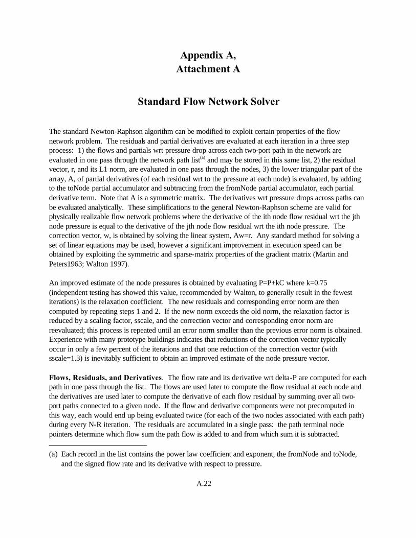
A.22

Appendix A, Attachment A

Standard Flow Network Solver The standard Newton-Raphson algorithm can be modified to exploit certain properties of the flow network problem. The residuals and partial derivatives are evaluated at each iteration in a three step process: 1) the flows and partials wrt pressure drop across each two-port path in the network are evaluated in one pass through the network path list(a) and may be stored in this same list, 2) the residual vector, r, and its L1 norm, are evaluated in one pass through the nodes, 3) the lower triangular part of the array, A, of partial derivatives (of each residual wrt to the pressure at each node) is evaluated, by adding to the toNode partial accumulator and subtracting from the fromNode partial accumulator, each partial derivative term. Note that A is a symmetric matrix. The derivatives wrt pressure drops across paths can be evaluated analytically. These simplifications to the general Newton-Raphson scheme are valid for physically realizable flow network problems where the derivative of the ith node flow residual wrt the jth node pressure is equal to the derivative of the jth node flow residual wrt the ith node pressure. The correction vector, w, is obtained by solving the linear system, Aw=r. Any standard method for solving a set of linear equations may be used, however a significant improvement in execution speed can be obtained by exploiting the symmetric and sparse-matrix properties of the gradient matrix (Martin and Peters1963; Walton 1997). An improved estimate of the node pressures is obtained by evaluating P=P+kC where k=0.75 (independent testing has showed this value, recommended by Walton, to generally result in the fewest iterations) is the relaxation coefficient. The new residuals and corresponding error norm are then computed by repeating steps 1 and 2. If the new norm exceeds the old norm, the relaxation factor is reduced by a scaling factor, sscale, and the correction vector and corresponding error norm are reevaluated; this process is repeated until an error norm smaller than the previous error norm is obtained. Experience with many prototype buildings indicates that reductions of the correction vector typically occur in only a few percent of the iterations and that one reduction of the correction vector (with sscale=1.3) is inevitably sufficient to obtain an improved estimate of the node pressure vector. Flows, Residuals, and Derivatives. The flow rate and its derivative wrt delta-P are computed for each path in one pass through the list. The flows are used later to compute the flow residual at each node and the derivatives are used later to compute the derivative of each flow residual by summing over all two-port paths connected to a given node. If the flow and derivative components were not precomputed in this way, each would end up being evaluated twice (for each of the two nodes associated with each path) during every N-R iteration. The residuals are accumulated in a single pass: the path terminal node pointers determine which flow sum the path flow is added to and from which sum it is subtracted. (a) Each record in the list contains the power law coefficient and exponent, the fromNode and toNode,

and the signed flow rate and its derivative with respect to pressure.

A.23

Derivatives, aij (ith zone flow wrt the jth node pressure), are accumulated in a similar manner during the

same pass through the path list. Note that path pressure drop is based on zone base pressures corrected for relative path elevation and zone air densities.

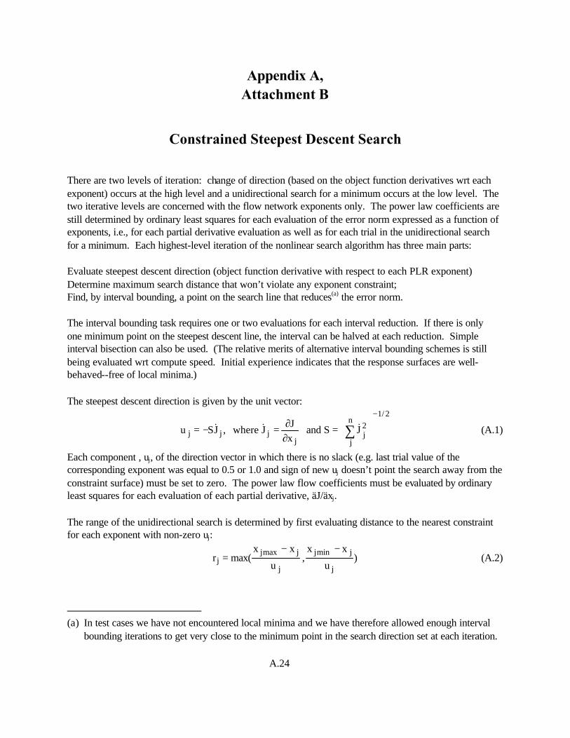
A.24

Appendix A, Attachment B

Constrained Steepest Descent Search There are two levels of iteration: change of direction (based on the object function derivatives wrt each exponent) occurs at the high level and a unidirectional search for a minimum occurs at the low level. The two iterative levels are concerned with the flow network exponents only. The power law coefficients are still determined by ordinary least squares for each evaluation of the error norm expressed as a function of exponents, i.e., for each partial derivative evaluation as well as for each trial in the unidirectional search for a minimum. Each highest-level iteration of the nonlinear search algorithm has three main parts: Evaluate steepest descent direction (object function derivative with respect to each PLR exponent) Determine maximum search distance that won’t violate any exponent constraint; Find, by interval bounding, a point on the search line that reduces(a) the error norm. The interval bounding task requires one or two evaluations for each interval reduction. If there is only one minimum point on the steepest descent line, the interval can be halved at each reduction. Simple interval bisection can also be used. (The relative merits of alternative interval bounding schemes is still being evaluated wrt compute speed. Initial experience indicates that the response surfaces are well-behaved--free of local minima.) The steepest descent direction is given by the unit vector:

2/1n

j

2j

jjjj JSand

xJ

Jwhere,JSu

−

=

∂∂=−= ∑ &&& (A.1)

Each component , uj, of the direction vector in which there is no slack (e.g. last trial value of the corresponding exponent was equal to 0.5 or 1.0 and sign of new uj doesn’t point the search away from the constraint surface) must be set to zero. The power law flow coefficients must be evaluated by ordinary least squares for each evaluation of each partial derivative, äJ/äxj. The range of the unidirectional search is determined by first evaluating distance to the nearest constraint for each exponent with non-zero uj:

)u

xx,

u

xxmax(r

j

jminj

j

jmaxjj

−−= (A.2)

(a) In test cases we have not encountered local minima and we have therefore allowed enough interval

bounding iterations to get very close to the minimum point in the search direction set at each iteration.

A.25

and selecting the minimum of these distance, ignoring no-slack (rj = 0) components, to be the maximum feasible range: R = min(r1, r2,..., rn) (A.3) However, if R is greater than the previous value of R, the previous value is used. A simple adaptive ranging algorithm has been developed to reduce R as the search progresses towards convergence The unidirectional search routine evaluates the object function for a series of diminishing distances, d, starting with d = R. The object function, J(x + ud), is evaluated at each new distance and a test of recent (J,d) pairs determines on which side of d the minimum lies. The routine successively reduces the mini-mum-bracketing interval (as long as the object function continues to drop) until a specified interval reduc-tion (typically 0.001) is reached.

Appendix B

Newton-Raphson Application Details

B.1

Appendix B

Newton-Raphson Application Details

B.1 Standard Airflow Network Solver A Newton-Raphson algorithm is used with a few special features that speed convergence by exploiting certain properties peculiar to network problems. The residuals and partial derivatives are evaluated at each iteration in a three-step process: 1. The flows and partials were pressure drop across each link in the network are evaluated in one pass

through the network description (a vector of link-property structures) and may be stored in this same struct vector.

2. The residuals, D, and their L1 error norm, ENORM, are evaluated in one pass through the nodes. 3. The lower triangular part of the array, A, of partial derivatives of each residual with respect to the

pressure at each node with index less than or equal to the residual node index is evaluated; A is the positive definite symmetric gradient matrix.

This simplification of the Newton-Raphson method is generally valid for physically realizable network problems where the derivative of the ith node residual flow with respect to the jth node pressure is equal to the derivative of the jth node residual flow with respect to the ith node pressure. The correction vector, C, is obtained by solving the linear system, AC=D. Any standard method of solving sets of linear equations may be used. However a significant improvement in execution speed can be obtained by exploiting the symmetric and sparse-matrix properties of the gradient matrix (1963, Walton 1997). An improved estimate of the node pressures is obtained by evaluating P=P+kC where k=0.75 is the relaxation coefficient. Testing showed this value, recommended by Walton, to generally result in the fewest iterations. The new residuals and corresponding error norm are then computed by repeating steps 1 and 2. If the new norm exceeds the old norm, the relaxation factor is reduced by a scaling factor, sscale, and the correction vector and corresponding error norm are reevaluated; this process is repeated until an error norm smaller than the previous error norm is obtained. Experience with many prototype buildings indicates that reductions of the correction vector typically occur in only a few percent of the iterations and that one reduction of the correction vector (with sscale=1.3) is inevitably sufficient to obtain an improved estimate of the node pressure vector. Flows, Residuals, and Derivatives. The flow rate and its derivative with respect to delta-P on each link are computed in one pass through the list. The flows are used later to compute the flow residual at each node and the derivatives are used later to compute the derivative of each flow residual by summing across all links connected to a given node. If the flow and derivative components were not precomputed in this

B.2

way, each would end up being evaluated twice (once for each of the two nodes associated with each link) during each N-R iteration. The residuals are accumulated in a single pass: the link terminal node pointers determine which flow sums the link flow is added to or subtracted from. The derivatives (ith zone flow with respect to the iD

th node pressure) are accumulated in a similar manner during the same pass through the net link vector. Note that link pressure difference is based on zone base pressures corrected for relative link elevations and zone air densities.

B.2 Constrained Steepest Descent Search There are two levels of iteration: change of direction (based on the object function derivatives with respect to each exponent) occurs at the high level and a unidirectional search for a minimum occurs at the low level. The two-level iterative search is concerned with the flow network exponents only. The power law coefficients are still determined by ordinary least squares for each evaluation of the error norm expressed as a function of exponents—i.e., for each partial derivative evaluation as well as for each trial in the unidirectional search for a minimum. The nonlinear search algorithm thus has three main parts: 1. Evaluate steepest descent direction (object function derivative with respect to each PLR exponent). 2. Determine maximum search distance that will not violate any exponent constraint. 3. Find, by interval bounding, a point on the search line that reduces(a) the error norm. The interval bounding task requires one or two evaluations for each interval reduction. If there is only one minimum point on the steepest descent line, the interval can be halved at each reduction. Simple interval bisection can also be used. (The relative merits of alternative interval bounding schemes are still being evaluated with respect to compute speed. Initial experience indicates that the response surfaces are well-behaved, free of local minima.) The steepest descent direction is given by the unit vector:

2/1n

n

2j

jjjj JSand

xJ

Jwhere,SJu−

=

∂∂=−= ∑ (B.1)

Each component, uj, of the direction vector in which there is no slack (e.g., last trial value of the corresponding exponent was equal to 0.5 or 1.0 and sign of new uj does not point the search away from the constraint surface) must be set to zero. The power-law flow coefficients must be evaluated by ordinary least squares for each evaluation of each partial derivative, äJ/äxj.

(a) Even a small norm reduction along each unidirectional search is usually sufficient for eventual

convergence. However, in test cases, we have not encountered local minima. We have, therefore, allowed enough interval iterations to get very close to the minimum point in the direction set at each iteration.

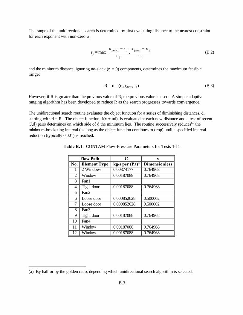
B.3

The range of the unidirectional search is determined by first evaluating distance to the nearest constraint for each exponent with non-zero uj:

−−=

j

jminj

j

jmaxjj u

xx,

u

xxmaxr (B.2)

and the minimum distance, ignoring no-slack (rj = 0) components, determines the maximum feasible range: R = min(r1, r2,..., rn) (B.3) However, if R is greater than the previous value of R, the previous value is used. A simple adaptive ranging algorithm has been developed to reduce R as the search progresses towards convergence. The unidirectional search routine evaluates the object function for a series of diminishing distances, d, starting with d = R. The object function, J(x + ud), is evaluated at each new distance and a test of recent (J,d) pairs determines on which side of d the minimum lies. The routine successively reduces(a) the minimum-bracketing interval (as long as the object function continues to drop) until a specified interval reduction (typically 0.001) is reached.

Table B.1. CONTAM Flow-Pressure Parameters for Tests 1-11

Flow Path C x No. Element Type kg/s per (Pa)x Dimensionless

1 2 Windows 0.00374177 0.764968 2 Window 0.00187088 0.764968 3 Fan1 4 Tight door 0.00187088 0.764968 5 Fan2 6 Loose door 0.000852628 0.500002 7 Loose door 0.000852628 0.500002 8 Fan3 9 Tight door 0.00187088 0.764968

10 Fan4 11 Window 0.00187088 0.764968 12 Window 0.00187088 0.764968

(a) By half or by the golden ratio, depending which unidirectional search algorithm is selected.

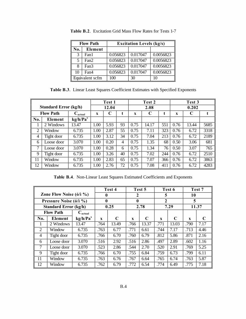
B.4

Table B.2. Excitation Grid Mass Flow Rates for Tests 1-7

Flow Path Excitation Levels (kg/s) No. Element

3 Fan1 0.056823 0.017047 0.0056823 5 Fan2 0.056823 0.017047 0.0056823 8 Fan3 0.056823 0.017047 0.0056823

10 Fan4 0.056823 0.017047 0.0056823 Equivalent scfm 100 30 10

Table B.3. Linear Least Squares Coefficient Estimates with Specified Exponents

Test 1 Test 2 Test 3 Standard Error (kg/h) 12.04 2.08 0.202 Flow Path Cactual x C t x C t x C t

No. Element kg/h/Pax 1 2 Windows 13.47 1.00 5.93 93 0.75 14.17 551 0.76 13.44 5685 2 Window 6.735 1.00 2.87 55 0.75 7.11 323 0.76 6.72 3318 4 Tight door 6.735 1.00 3.12 34 0.75 7.04 213 0.76 6.72 2189 6 Loose door 3.070 1.00 0.20 4 0.75 1.35 68 0.50 3.06 681 7 Loose door 3.070 1.00 0.28 6 0.75 1.34 76 0.50 3.07 765 9 Tight door 6.735 1.00 3.26 40 0.75 7.02 244 0.76 6.72 2510

11 Window 6.735 1.00 2.83 65 0.75 7.07 366 0.76 6.72 3863 12 Window 6.735 1.00 2.76 72 0.75 7.08 411 0.76 6.72 4283

Table B.4. Non-Linear Least Squares Estimated Coefficients and Exponents

Test 4 Test 5 Test 6 Test 7 Zone Flow Noise (ó/ì %) 0 2 5 10 Pressure Noise (ó/ì %) 0 0 2 5 Standard Error (kg/h) 0.25 2.78 7.29 11.37 Flow Path Cactual

No. Element kg/h/Pax x C x C x C x C 1 2 Windows 13.47 .764 13.49 .766 13.37 .771 13.03 .790 7.17 2 Window 6.735 .763 6.77 .771 6.61 .744 7.17 .713 4.46 4 Tight door 6.735 .766 6.70 .760 6.79 .812 5.86 .871 2.16 6 Loose door 3.070 .516 2.92 .516 2.86 .497 2.89 .602 1.16 7 Loose door 3.070 .523 2.86 .544 2.70 .520 2.91 .769 5.25 9 Tight door 6.735 .766 6.70 .755 6.84 .759 6.73 .799 6.11

11 Window 6.735 .763 6.76 .767 6.64 .765 6.74 .763 5.87 12 Window 6.735 .762 6.79 .772 6.54 .774 6.49 .775 7.18

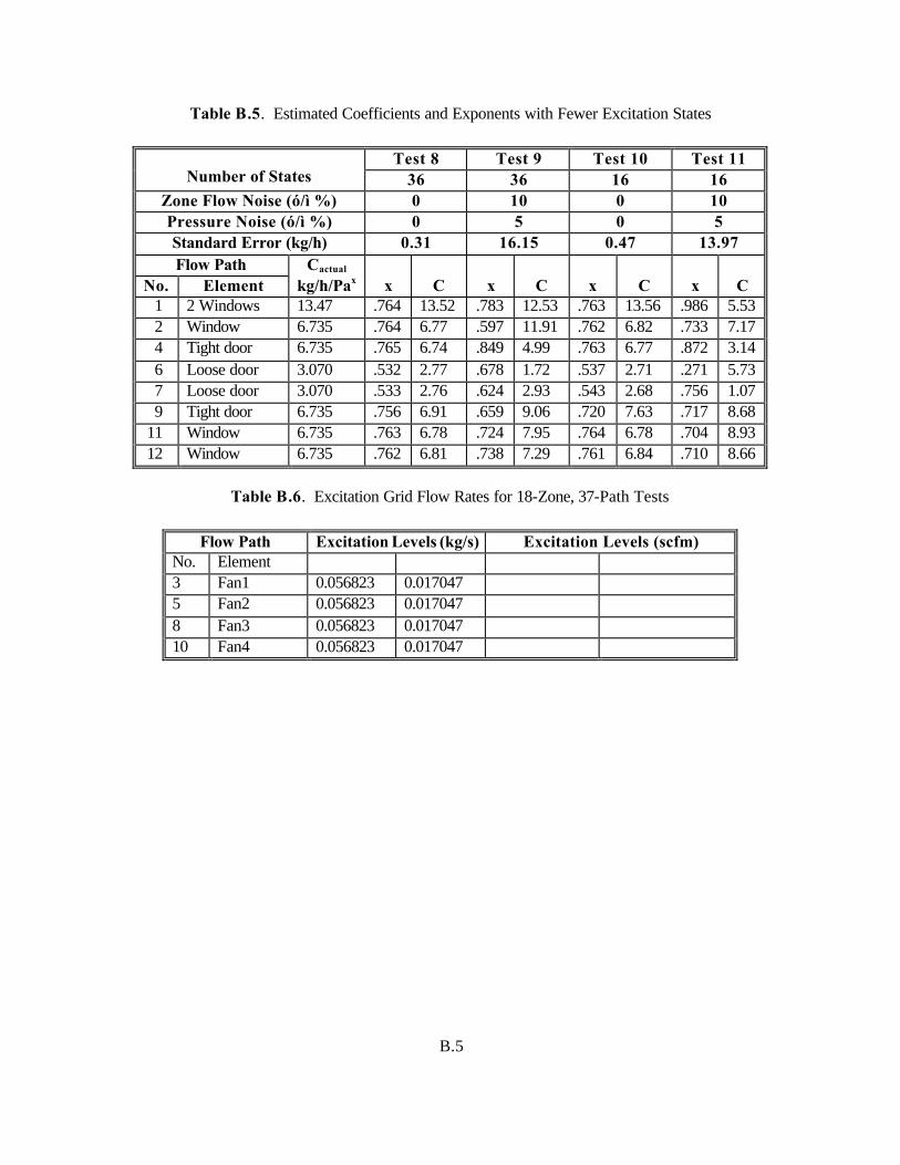
B.5

Table B.5. Estimated Coefficients and Exponents with Fewer Excitation States

Test 8 Test 9 Test 10 Test 11 Number of States 36 36 16 16

Zone Flow Noise (ó/ì %) 0 10 0 10 Pressure Noise (ó/ì %) 0 5 0 5 Standard Error (kg/h) 0.31 16.15 0.47 13.97 Flow Path Cactual

No. Element kg/h/Pax x C x C x C x C 1 2 Windows 13.47 .764 13.52 .783 12.53 .763 13.56 .986 5.53 2 Window 6.735 .764 6.77 .597 11.91 .762 6.82 .733 7.17 4 Tight door 6.735 .765 6.74 .849 4.99 .763 6.77 .872 3.14 6 Loose door 3.070 .532 2.77 .678 1.72 .537 2.71 .271 5.73 7 Loose door 3.070 .533 2.76 .624 2.93 .543 2.68 .756 1.07 9 Tight door 6.735 .756 6.91 .659 9.06 .720 7.63 .717 8.68

11 Window 6.735 .763 6.78 .724 7.95 .764 6.78 .704 8.93 12 Window 6.735 .762 6.81 .738 7.29 .761 6.84 .710 8.66

Table B.6. Excitation Grid Flow Rates for 18-Zone, 37-Path Tests

Flow Path Excitation Levels (kg/s) Excitation Levels (scfm) No. Element 3 Fan1 0.056823 0.017047 5 Fan2 0.056823 0.017047 8 Fan3 0.056823 0.017047 10 Fan4 0.056823 0.017047

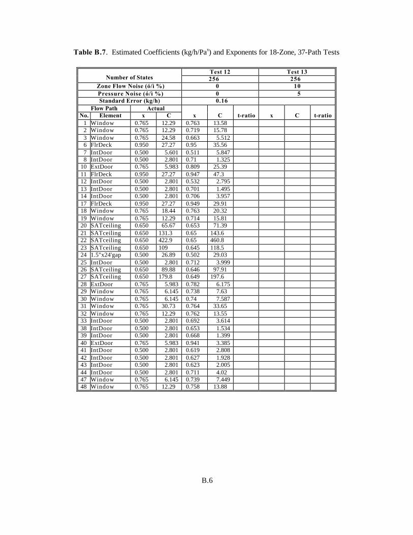
B.6

Table B.7. Estimated Coefficients (kg/h/Pax) and Exponents for 18-Zone, 37-Path Tests

Test 12 Test 13 Number of States 256 256

Zone Flow Noise (ó/ì %) 0 10 Pressure Noise (ó/ì %) 0 5 Standard Error (kg/h) 0.16

Flow Path Actual No. Element x C x C t-ratio x C t-ratio

1 Window 0.765 12.29 0.763 13.58 2 Window 0.765 12.29 0.719 15.78 3 Window 0.765 24.58 0.663 5.512 6 FlrDeck 0.950 27.27 0.95 35.56 7 IntDoor 0.500 5.601 0.511 5.847 8 IntDoor 0.500 2.801 0.71 1.325

10 ExtDoor 0.765 5.983 0.809 25.39 11 FlrDeck 0.950 27.27 0.947 47.3 12 IntDoor 0.500 2.801 0.532 2.795 13 IntDoor 0.500 2.801 0.701 1.495 14 IntDoor 0.500 2.801 0.706 3.957 17 FlrDeck 0.950 27.27 0.949 29.91 18 Window 0.765 18.44 0.763 20.32 19 Window 0.765 12.29 0.714 15.81 20 SATceiling 0.650 65.67 0.653 71.39 21 SATceiling 0.650 131.3 0.65 143.6 22 SATceiling 0.650 422.9 0.65 460.8 23 SATceiling 0.650 109 0.645 118.5 24 1.5"x24'gap 0.500 26.89 0.502 29.03 25 IntDoor 0.500 2.801 0.712 3.999 26 SATceiling 0.650 89.88 0.646 97.91 27 SATceiling 0.650 179.8 0.649 197.6 28 ExtDoor 0.765 5.983 0.782 6.175 29 Window 0.765 6.145 0.738 7.63 30 Window 0.765 6.145 0.74 7.587 31 Window 0.765 30.73 0.764 33.65 32 Window 0.765 12.29 0.762 13.55 33 IntDoor 0.500 2.801 0.692 3.614 38 IntDoor 0.500 2.801 0.653 1.534 39 IntDoor 0.500 2.801 0.668 1.399 40 ExtDoor 0.765 5.983 0.941 3.385 41 IntDoor 0.500 2.801 0.619 2.808 42 IntDoor 0.500 2.801 0.627 1.928 43 IntDoor 0.500 2.801 0.623 2.005 44 IntDoor 0.500 2.801 0.711 4.02 47 Window 0.765 6.145 0.739 7.449 48 Window 0.765 12.29 0.758 13.88

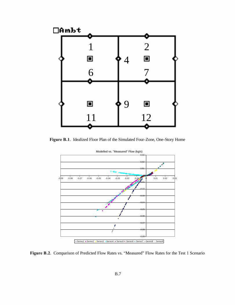
B.7

12

7

14

2

6

119

Figure B.1. Idealized Floor Plan of the Simulated Four-Zone, One-Story Home

Modelled vs. "Measured" Flow (kg/s)

-0.09

-0.08

-0.07

-0.06

-0.05

-0.04

-0.03

-0.02

-0.01

0

0.01

0.02

0.03

-0.09 -0.08 -0.07 -0.06 -0.05 -0.04 -0.03 -0.02 -0.01 0 0.01 0.02 0.03

Series1 Series2 Series3 Series4 Series5 Series6 Series7 Series8 Series9

Figure B.2. Comparison of Predicted Flow Rates vs. “Measured” Flow Rates for the Test 1 Scenario

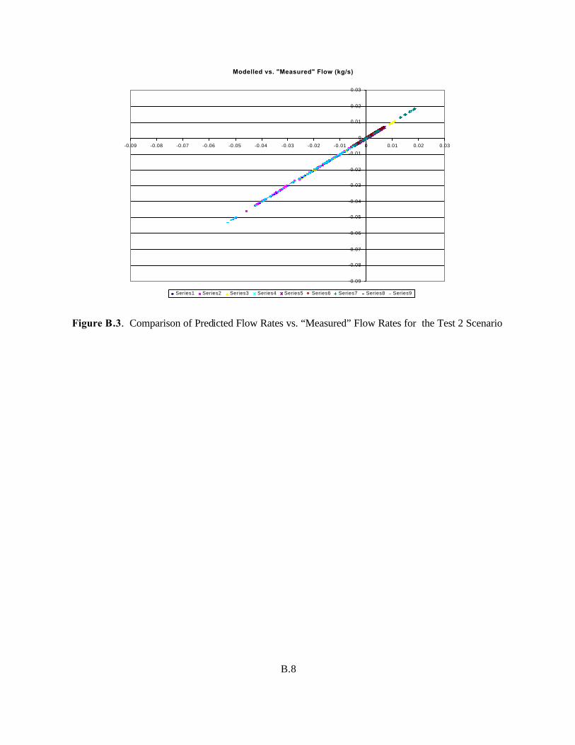
B.8

Modelled vs. "Measured" Flow (kg/s)

-0.09

-0.08

-0.07

-0.06

-0.05

-0.04

-0.03

-0.02

-0.01

0

0.01

0.02

0.03

-0.09 -0.08 -0.07 -0.06 -0.05 -0.04 -0.03 -0.02 -0.01 0 0.01 0.02 0.03

Series1 Series2 Series3 Series4 Series5 Series6 Series7 Series8 Series9

Figure B.3. Comparison of Predicted Flow Rates vs. “Measured” Flow Rates for the Test 2 Scenario

Appendix C

Example Biological Health Effect Database (BHED) for Biological Agents

Appendix C

Example Biological Health Effect Database (BHED) for Biological Agents

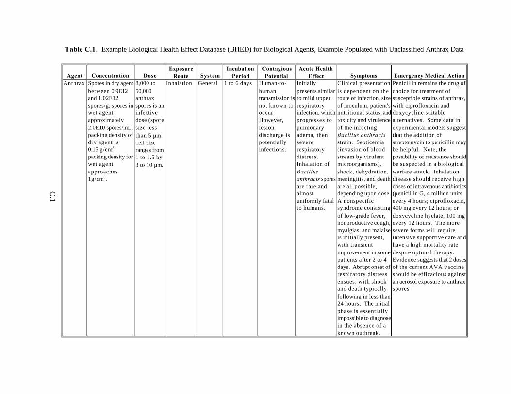
C.1

Table C.1. Example Biological Health Effect Database (BHED) for Biological Agents, Example Populated with Unclassified Anthrax Data

Agent Concentration Dose Exposure

Route System Incubation

Period Contagious Potential

Acute Health Effect Symptoms Emergency Medical Action

Anthrax Spores in dry agent between 0.9E12 and 1.02E12 spores/g; spores in wet agent approximately 2.0E10 spores/mL; packing density of dry agent is 0.15 g/cm3; packing density for wet agent approaches 1g/cm3.

8,000 to 50,000 anthrax spores is an infective dose (spore size less than 5 µm; cell size ranges from 1 to 1.5 by 3 to 10 µm.

Inhalation General 1 to 6 days Human-to-human transmission is not known to occur. However, lesion discharge is potentially infectious.

Initially presents similar to mild upper respiratory infection, which progresses to pulmonary adema, then severe respiratory distress. Inhalation of Bacillus anthracis spores are rare and almost uniformly fatal to humans.

Clinical presentation is dependent on the route of infection, size of inoculum, patient's nutritional status, and toxicity and virulence of the infecting Bacillus anthracis strain. Septicemia (invasion of blood stream by virulent microorganisms), shock, dehydration, meningitis, and death are all possible, depending upon dose. A nonspecific syndrome consisting of low-grade fever, nonproductive cough, myalgias, and malaise is initially present, with transient improvement in some patients after 2 to 4 days. Abrupt onset of respiratory distress ensues, with shock and death typically following in less than 24 hours . The initial phase is essentially impossible to diagnose in the absence of a known outbreak.

Penicillin remains the drug of choice for treatment of susceptible strains of anthrax, with ciprofloxacin and doxycycline suitable alternatives. Some data in experimental models suggest that the addition of streptomycin to penicillin may be helpful. Note, the possibility of resistance should be suspected in a biological warfare attack. Inhalation disease should receive high doses of intravenous antibiotics (penicillin G, 4 million units every 4 hours; ciprofloxacin, 400 mg every 12 hours; or doxycycline hyclate, 100 mg every 12 hours. The more severe forms will require intensive supportive care and have a high mortality rate despite optimal therapy. Evidence suggests that 2 doses of the current AVA vaccine should be efficacious against an aerosol exposure to anthrax spores

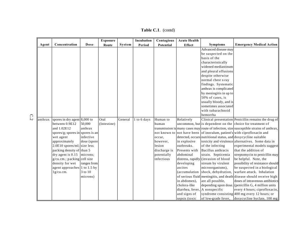
C.2

Table C.1. (contd)

Agent Concentration Dose Exposure

Route System Incubation

Period Contagious Potential

Acute Health Effect Symptoms Emergency Medical Action

Advanced disease may be suspected on the basis of the characteristically widened mediastinum and pleural effusions despite otherwise normal chest x-ray findings. Systematic anthrax is complicated by meningitis in up to 50% of cases, is usually bloody, and is sometimes associated with subarachnoid hemorrha

anthrax spores in dry agent between 0.9E12 and 1.02E12 spores/g; spores in wet agent approximately 2.0E10 spores/ml; packing density of dry agent is 0.15 g/cu.cm.; packing density for wet agent approaches 1g/cu.cm.

8,000 to 50,000 anthrax spores is an infective dose (spore size less than 5 microns; cell size ranges from 1 to 1.5 by 3 to 10 microns)

Oral (Intestine)

General 1 to 6 days Human to human transmission is not known to occur, however, lesion discharge is potentially infectious

Relatively uncommon, but many cases may not have been detected, occurs in explosive outbreaks. Presents with abdominal distress, rapidly developing ascites (accumulation of serious fluid in abdomen), cholera -like diarrhea, fever, and signs of sepsis (toxic

Clinical presentation is dependent on the route of infection, size of inoculum, patient's nutritional status, and toxicity and virulence of the infecting Bacillus anthracis strain. Septicemia (invasion of blood stream by virulent microorganisms), shock, dehydration, meningitis, and death are all possible, depending upon dose. A nonspecific syndrome consisting of low-grade fever,

Penicillin remains the drug of choice for treatment o f susceptible strains of anthrax, with ciprofloxacin and doxycycline suitable alternatives. Some data in experimental models suggest that the addition of streptomycin to penicillin may be helpful. Note, the possibility of resistance should be suspected in a biological warfare attack. Inhalation disease should receive high doses of intravenous antibiotics (penicillin G, 4 million units every 4 hours; ciprofloxacin, 400 mg every 12 hours; or doxycycline hyclate, 100 mg

C.3

Table C.1. (contd)

Agent Concentration Dose Exposure

Route System Incubation

Period Contagious Potential

Acute Health Effect Symptoms Emergency Medical Action

condition resulting from spread of bacteria).

nonproductive cough, myalgias, and malaise is initially present, with transient improvement in some patients after 2 to 4 days. Abrupt onset of respiratory distress ensues, with shock and death typically following in less than 24 hours. The initial phase is essentially impossible to diagnose in the absence of a known outbreak. Advanced disease may be suspected on the basis of the characteristically widened mediastinum and pleural effusions despite otherwise normal chest x-ray findings. Systematic anthrax is complicated by meningitis in up to 50% of cases, is usually bloddy, and is sometimes associated with subarachnoid hemorrha

every 12 hours. The more severe forms will require intensive supportive care and have a high mortality rate despite optimal therapy. Evidence suggests that 2 doses of the current AVA vaccine should b e efficacious against an aerosol exposure to anthrax spores

C.4

Table C.1. (contd)

Agent Concentration Dose Exposure

Route System Incubation

Period Contagious Potential

Acute Health Effect Symptoms Emergency Medical Action

anthrax spores in dry agent between 0.9E12 and 1.02E12 spores/g; spores in wet agent approximately 2.0E10 spores/ml; packing density of dry agent is 0.15 g/cu.cm.; packing density for wet agent approaches 1g/cu.cm.

8,000 to 50,000 anthrax spores is an infective dose (spore size less than 5 microns; cell size ranges from 1 to 1.5 by 3 to 10 microns)

Dermal (Cutaneous)

General 1 to 6 days Human to human transmission is not known to occur, however, lesion discharge is potentially infectious

Most common form, occurring in approximately 95% of patients. Presents with itching (first 2 to 3 hours), followed by a papular, then vesiculated lesion. The mildest cutaneous form develops a necrotic eschar (36 hours) that falls off without scarring. The most serious form, malignant edema, forms an aschar which is surrounded by grossly edematous tissue (2 to 6 days) with necrosis and blistering

Clinical presentation is dependent on the route of infection, size of inoculum, patient's nutritional status, and toxicity and virulence of the infecting Bacillus anthracis strain. Septicemia (invasion of blood stream by virulent microorganisms), shock, dehydration, meningitis, and death are all possible, depending upon dose. A nonspecific syndrome consisting of low-grade fever, nonproductive cough, myalgias, and malaise is initially present, with transient improvement in some patients after 2 to 4 days. Abrupt onset of respiratory distress ensues, with shock and death typically following in less than 24 hours. The initial phase is essentially impossible to diagnose in the absence of a

Penicillin remains the drug of choice for treatment of susceptible strains of anthrax, with ciprofloxacin and doxycycline suitable alternatives. Some data in experimental models suggest that the addition of streptomycin to penicillin may be helpful. Note, the possibility of resistance should be suspected in a biological warfare attack. Inhalation disease should receive high doses of intravenous antibiotics (penicillin G, 4 million units every 4 hours; ciprofloxacin, 400 mg every 12 hours; or doxycycline hyclate, 100 mg every 12 hours. The more severe forms will require intensive supportive care and have a high mortality rate despite optimal therapy. Evidence suggests that 2 doses of the current AVA vaccine should be efficacious against an aerosol exposure to anthrax spores

C.5

Table C.1. (contd)

Agent Concentration Dose Exposure

Route System Incubation

Period Contagious Potential

Acute Health Effect Symptoms Emergency Medical Action

known outbreak. Advanced disease may be suspected on the basis of the characteristically widened mediastinum and pleural effusions despite otherwise normal chest x-ray findings. Systematic anthrax is complicated by meningitis in up to 50% of cases, is usually bloddy, and is sometimes associated with subarachnoid hemorrha

anthrax spores in dry agent between 0.9E12 and 1.02E12 spores/g; spores in wet agent approximately 2.0E10 spores/ml; packing density of dry agent is 0.15 g/cu.cm.; packing density for wet agent approaches 1g/cu.cm.

Acute exposure - all routes

Cardiovascular

1 to 6 days Severe hypotension (abnormally low blood pressure) and shock may result from all routes of anthrax infection. Tachycardia (rapid heart rate) is common

Clinical presentation is dependent on the route of infection, size of inoculum, patient's nutritional status, and toxicity and virulence of the infecting Bacillus anthracis strain. Septicemia (invasion of blood stream by virulent microorganisms), shock, dehydration, meningitis, and death are all possible, depending upon dose. A nonspecific syndrome consisting

Penicillin remains the drug of choice for treatment of susceptible strains of anthrax, with ciprofloxacin and doxycycline suitable alternatives. Some data in experimental models suggest that the addition of streptomycin to penicillin may be helpful. Note, the possibility of resistance should be suspected in a biological warfare attack. Inhalation disease should receive high doses of intravenous antibiotics (penicillin G, 4 million units every 4 hours; ciprofloxacin, 400 mg every 12 hours; or

C.6

Table C.1. (contd)

Agent Concentration Dose Exposure

Route System Incubation

Period Contagious Potential

Acute Health Effect Symptoms Emergency Medical Action

of low-grade fever, nonproductive cough, myalgias, and malaise is initially present, with transient improvement in some patients after 2 to 4 days. Abrupt onset of respiratory distress ensues, with shock and death typically following in less than 24 hours. The initial phase is essentially impossible to diagnose in the absence of a known outbreak. Advanced disease may be suspected on the basis of the characteristically widened mediastinum and pleural effusions despite otherwise normal chest x-ray findings. Systematic anthrax is complicated by meningitis in up to 50% of cases, is usually bloddy, and is sometimes associated with subarachnoid hemorrha

doxycycline hyclate, 100 mg every 12 hours. The more severe forms will require intensive supportive care and have a high mortality rate despite optimal therapy. Evidence suggests that 2 doses of the current AVA vaccine should be efficacious against an aerosol exposure to anthrax spores

C.7

Table C.1. (contd)

Agent Concentration Dose Exposure

Route System Incubation

Period Contagious Potential

Acute Health Effect Symptoms Emergency Medical Action

anthrax spores in dry agent between 0.9E12 and 1.02E12 spores/g; spores in wet agent approximately 2.0E10 spores/ml; packing density of dry agent is 0.15 g/cu.cm.; packing density for wet agent approaches 1g/cu.cm.

Cell size ranges from 1 to 1.5 by 3 to 10 microns

Acute exposure - all routes

Respiratory

1 to 6 days Extensive edema and tracheal compression with severe respiratory distress is most common following inhalation of anthrax spores , but may occur from all routes of infection. Respiratory symptoms develop in a biphasic pattern, with flu-like respiratory symptoms first, followed by sudden respiratory distress. This is almost always fatal.

Clinical presentation is dependent on the route of infection, size of inoculum, patient's nutritional status, and toxicity and virulence of the infecting Bacillus anthracis strain. Septicemia (invasion of blood stream by virulent microorganisms), shock, dehydration, meningitis, and death are all possible, depending upon dose. A nonspecific syndrome consisting of low-grade fever, nonproductive cough, myalgias, and malaise is initially present, with transient improvement in some patients after 2 to 4 days. Abrupt onset of respiratory distress ensues, with shock and death typically following in less than 24 hours. The initial phase is essentially impossible to diagnose in the absence of a

Penicillin remains the drug of choice for treatment of susceptible strains of anthrax, with ciprofloxacin and doxycycline suitable alternatives. Some data in experimental models suggest that the addition of streptomycin to penicillin may be helpful. Note, the possibility of resistance should be suspected in a biological warfare attack. Inhalation disease should receive high doses of intravenous antibiotics (penicillin G, 4 million units every 4 hours; ciprofloxacin, 400 mg every 12 hours; or doxycycline hyclate, 100 mg every 12 hours. The more severe forms will require intensive supportive care and have a high mortality rate despite optimal therapy. Evidence suggests that 2 doses of the current AVA vaccine should be efficacious against an aerosol exposure to anthrax spores

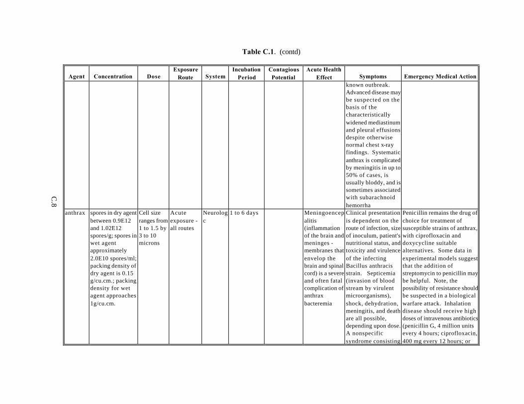
C.8

Table C.1. (contd)

Agent Concentration Dose Exposure

Route System Incubation

Period Contagious Potential

Acute Health Effect Symptoms Emergency Medical Action

known outbreak. Advanced disease may be suspected on the basis of the characteristically widened mediastinum and pleural effusions despite otherwise normal chest x-ray findings. Systematic anthrax is complicated by meningitis in up to 50% of cases, is usually bloddy, and is sometimes associated with subarachnoid hemorrha

anthrax spores in dry agent between 0.9E12 and 1.02E12 spores/g; spores in wet agent approximately 2.0E10 spores/ml; packing density of dry agent is 0.15 g/cu.cm.; packing density for wet agent approaches 1g/cu.cm.

Cell size ranges from 1 to 1.5 by 3 to 10 microns

Acute exposure - all routes

Neurologic

1 to 6 days Meningoencephalitis (inflammation of the brain and meninges - membranes that envelop the brain and spinal cord) is a severe and often fatal complication of anthrax bacteremia

Clinical presentation is dependent on the route of infection, size of inoculum, patient's nutritional status, and toxicity and virulence of the infecting Bacillus anthracis strain. Septicemia (invasion of blood stream by virulent microorganisms), shock, dehydration, meningitis, and death are all possible, depending upon dose. A nonspecific syndrome consisting

Penic illin remains the drug of choice for treatment of susceptible strains of anthrax, with ciprofloxacin and doxycycline suitable alternatives. Some data in experimental models suggest that the addition of streptomycin to penicillin may be helpful. Note, the possibility of resistance should be suspected in a biological warfare attack. Inhalation disease should receive high doses of intravenous antibiotics (penicillin G, 4 million units every 4 hours; ciprofloxacin, 400 mg every 12 hours; or

C.9

Table C.1. (contd)

Agent Concentration Dose Exposure

Route System Incubation

Period Contagious Potential

Acute Health Effect Symptoms Emergency Medical Action

of low-grade fever, nonproductive cough, myalgias, and malaise is initially present, with transient improvement in some patients after 2 to 4 days. Abrupt onset of respiratory distress ensues, with shock and death typically following in less than 24 hours. The initial phase is essentially impossible to diagnose in the absence of a known outbreak. Advanced disease may be suspected on the basis of the characteristically widened mediastinum and pleural effusions despite otherwise normal chest x-ray findings. Systematic anthrax is complicated by meningitis in up to 50% of cases, is usually bloddy, and is sometimes associated with subarachnoid hemorrha

doxycycline hyclate, 100 mg every 12 hours. The more severe forms will require intensive supportive care and have a high mortality rate despite optimal therapy. Evidence suggests that 2 doses of the current AVA vaccine should be efficacious against an aerosol exposure to anthrax spores

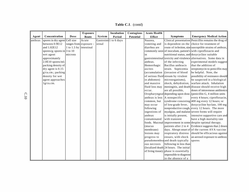
C.10

Table C.1. (contd)

Agent Concentration Dose Exposure

Route System Incubation

Period Contagious Potential

Acute Health Effect Symptoms Emergency Medical Action

anthrax spores in dry agent between 0.9E12 and 1.02E12 spores/g; spores in wet agent approximately 2.0E10 spores/ml; packing density of dry agent is 0.15 g/cu.cm.; packing density for wet agent approaches 1g/cu.cm.

Cell size ranges from 1 to 1.5 by 3 to 10 microns

Acute exposure - intestinal

Gastrointestinal

1 to 6 days Nausea, vomiting and diarrhea are commonly seen in gastrointestinal anthrax. Hemorrhagic ascites (accumulation of serious fluid in abdomen) and massive fluid loss may occur. Oropharyngeal anthrax is less common, but may occur following ingestions of anthrax contaminated foods. Mucosal (mucus membrane) lesions may progress to pseudomembranous necrosis (localized death of living tissue).

Clinical presentation is dependent on the route of in fection, size of inoculum, patient's nutritional status, and toxicity and virulence of the infecting Bacillus anthracis strain. Septicemia (invasion of blood stream by virulent microorganisms), shock, dehydration, meningitis, and death are all possible, depending upon dose. A nonspecific syndrome consisting of low-grade fever, nonproductive cough, myalgias, and malaise is initially present, with transient improvement in some patients after 2 to 4 days. Abrupt onset of respiratory distress ensues, with s hock and death typically following in less than 24 hours. The initial phase is essentially impossible to diagnose in the absence of a

Penicillin remains the drug of choice for treatment of susceptible strains of anthrax, with ciprofloxacin and doxycycline suitable alternatives. Some data in experimental models suggest that the addition of streptomycin to penicillin may be helpful. Note, the possibility of resistance should be suspected in a biological warfare attack. Inhalation disease should receive h igh doses of intravenous antibiotics (penicillin G, 4 million units every 4 hours; ciprofloxacin, 400 mg every 12 hours; or doxycycline hyclate, 100 mg every 12 hours. The more severe forms will require intensive supportive care and have a high mortality rate despite optimal therapy. Evidence suggests that 2 doses of the current AVA vaccine should be efficacious against an aerosol exposure to anthrax spores

C.11

Table C.1. (contd)

Agent Concentration Dose Exposure

Route System Incubation

Period Contagious Potential

Acute Health Effect Symptoms Emergency Medical Action

known outbreak. Advanced disease may be suspected on the basis of the characteristically widened mediastinum and pleural effusions despite otherwise normal chest x-ray findings. Systematic anthrax is complicated by meningitis in up to 50% of cases, is usually bloddy, and is sometimes associated with subarachnoid hemorrha

anthrax spores in dry agent between 0.9E12 and 1.02E12 spores/g; spores in wet agent approximately 2.0E10 spores/ml; packing density of dry agent is 0.15 g/cu.cm.; packing density for wet agent approaches 1g/cu.cm.

Cell size ranges from 1 to 1.5 by 3 to 10 microns

Acute exposure - all routes

Hepatic 1 to 6 days Jaundice has been reported in some patients with anthrax bacteremia

Clinical presentation is dependent on the route of infection, size of inoculum, patient's nutritional status, and toxicity and virulence of the infecting Bacillus anthracis strain. Septicemia (invasion of blood stream by virulent microorganisms), shock, dehydration, meningitis, and death are all possible, depending upon dose. A nonspecific syndrome consisting

Penicillin remains the drug of choice for treatment of susceptible strains of anthrax, with ciprofloxacin and doxycycline suitable alternatives. Some data in experimental models suggest that the addition of streptomycin to penicillin may be helpful. Note, the possibility of resistance should be suspected in a biological warfare attack. Inhalation disease should receive high doses of intravenous antibiotics (penicillin G, 4 million units every 4 hours; ciprofloxacin, 400 mg every 12 hours; or

C.12

Table C.1. (contd)

Agent Concentration Dose Exposure

Route System Incubation

Period Contagious Potential

Acute Health Effect Symptoms Emergency Medical Action

of low-grade fever, nonproductive cough, myalgias, and malaise is initially present, with transient improvement in some patients after 2 to 4 days. Abrupt onset of respiratory distress ensues, with shock and death typically following in less than 24 hours. The initial phase is essentially impossible to diagnose in the absence of a known outbreak. Advanced disease may be suspected on the basis of the characteristically widened mediastinum and pleural effusions des pite otherwise normal chest x-ray findings. Systematic anthrax is complicated by meningitis in up to 50% of cases, is usually bloddy, and is sometimes associated with subarachnoid hemorrha

doxycycline hyclate, 100 mg every 12 hours. The more severe forms will require intensive supportive care and have a high mortality rate despite optimal therapy. Evidence suggests that 2 doses of the current AVA vaccine should be efficacious against an aerosol exposure to anthrax spores

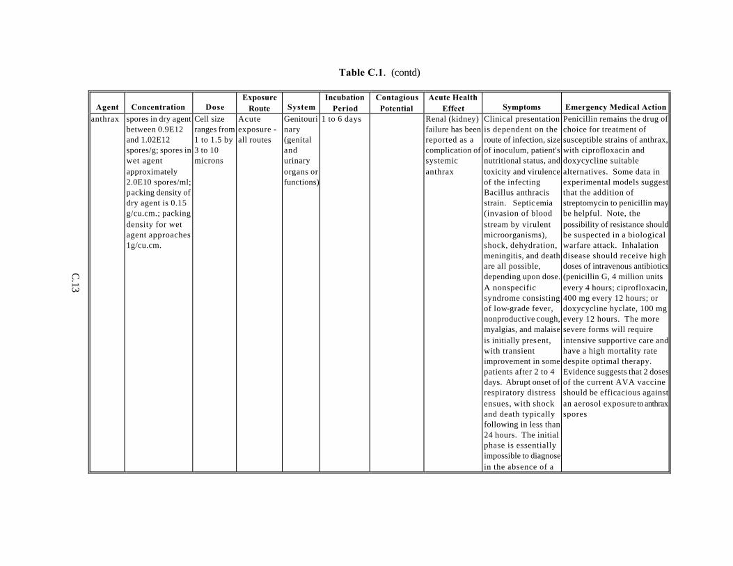
C.13

Table C.1. (contd)

Agent Concentration Dose Exposure

Route System Incubation

Period Contagious Potential

Acute Health Effect Symptoms Emergency Medical Action

anthrax spores in dry agent between 0.9E12 and 1.02E12 spores/g; spores in wet agent approximately 2.0E10 spores/ml; packing density of dry agent is 0.15 g/cu.cm.; packing density for wet agent approaches 1g/cu.cm.

Cell size ranges from 1 to 1.5 by 3 to 10 microns

Acute exposure - all routes

Genitourinary (genital and urinary organs or functions)

1 to 6 days Renal (kidney) failure has been reported as a complication of systemic anthrax

Clinical presentation is dependent on the route of infection, size of inoculum, patient's nutritional status, and toxicity and virulence of the infecting Bacillus anthracis strain. Septicemia (invasion of blood stream by virulent microorganisms), shock, dehydration, meningitis, and death are all possible, depending upon dose. A nonspecific syndrome consisting of low-grade fever, nonproductive cough, myalgias, and malaise is initially present, with transient improvement in some patients after 2 to 4 days. Abrupt onset of respiratory distress ensues, with shock and death typically following in less than 24 hours. The initial phase is essentially impossible to diagnose in the absence of a

Penicillin remains the drug of choice for treatment of susceptible strains of anthrax, with ciprofloxacin and doxycycline suitable alternatives. Some data in experimental models suggest that the addition of streptomycin to penicillin may be helpful. Note, the possibility of resistance should be suspected in a biological warfare attack. Inhalation disease should receive high doses of intravenous antibiotics (penicillin G, 4 million units every 4 hours; ciprofloxacin, 400 mg every 12 hours; or doxycycline hyclate, 100 mg every 12 hours. The more severe forms will require intensive supportive care and have a high mortality rate despite optimal therapy. Evidence suggests that 2 doses of the current AVA vaccine should be efficacious against an aerosol exposure to anthrax spores

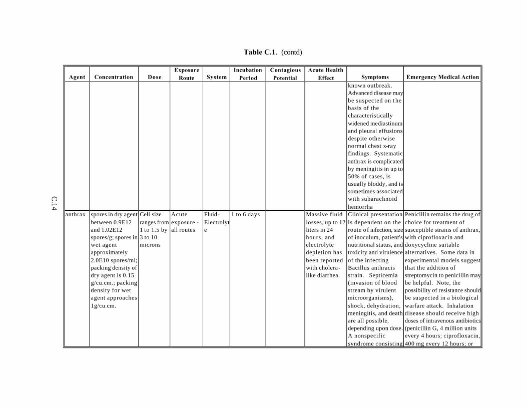
C.14

Table C.1. (contd)

Agent Concentration Dose Exposure

Route System Incubation

Period Contagious Potential

Acute Health Effect Symptoms Emergency Medical Action

known outbreak. Advanced disease may be suspected on t he basis of the characteristically widened mediastinum and pleural effusions despite otherwise normal chest x-ray findings. Systematic anthrax is complicated by meningitis in up to 50% of cases, is usually bloddy, and is sometimes associated with subarachnoid hemorrha

anthrax spores in dry agent between 0.9E12 and 1.02E12 spores/g; spores in wet agent approximately 2.0E10 spores/ml; packing density of dry agent is 0.15 g/cu.cm.; packing density for wet agent approaches 1g/cu.cm.

Cell size ranges from 1 to 1.5 by 3 to 10 microns

Acute exposure - all routes

Fluid-Electrolyte

1 to 6 days Massive fluid losses, up to 12 liters in 24 hours, and electrolyte depletion has been reported with cholera -like diarrhea.

Clinical presentation is dependent on the route o f infection, size of inoculum, patient's nutritional status, and toxicity and virulence of the infecting Bacillus anthracis strain. Septicemia (invasion of blood stream by virulent microorganisms), shock, dehydration, meningitis, and death are all possib le, depending upon dose. A nonspecific syndrome consisting

Penicillin remains the drug of choice for treatment of susceptible strains of anthrax, with ciprofloxacin and doxycycline suitable alternatives. Some data in experimental models suggest that the addition of streptomycin to penicillin may be helpful. Note, the possibility of resistance should be suspected in a biological warfare attack. Inhalation disease should receive high doses of intravenous antibiotics (penicillin G, 4 million units every 4 hours; ciprofloxacin, 400 mg every 12 hours; or

C.15

Table C.1. (contd)

Agent Concentration Dose Exposure

Route System Incubation

Period Contagious Potential

Acute Health Effect Symptoms Emergency Medical Action

of low-grade fever, nonproductive cough, myalgias, and malaise is initially present, with transient improvement in some patients after 2 to 4 days. Abrupt onset of respiratory distress ensues, with shock and death typically following in less than 24 hours. The initial phase is essentially impossible to diagnose in the absence of a known outbreak. Advanced disease may be suspected on the basis of the characteristically widened mediastinum and pleural effusions despite otherwise normal chest x-ray findings. Systematic anthrax is complicated by meningitis in up to 50% of cases, is usually bloddy, and is sometimes associated with subarachnoid hemorrha

doxycycline hyclate, 100 mg every 12 hours. The more severe forms will require intensive supportive care and have a high mortality rate despite optimal therapy. Evidence suggests that 2 doses of the current AVA vaccine should be efficacious against an aerosol exposure to anthrax spores

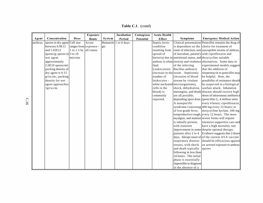
C.16

Table C.1. (contd)

Agent Concentration Dose Exposure

Route System Incubation

Period Contagious Potential

Acute Health Effect Symptoms Emergency Medical Action

anthrax spores in dry agent between 0.9E12 and 1.02E12 spores/g; spores in wet agent approximately 2.0E10 spores/ml; packing density of dry agent is 0.15 g/cu.cm.; packing density for wet agent approaches 1g/cu.cm.

Cell size ranges from 1 to 1.5 by 3 to 10 microns

Acute exposure - all routes

Hematologic

1 to 6 days Sepsis (toxic condition resulting from spread of bacteria) due to anthrax is often fatal. Leukocytosis (increase in the number of leukocytes - white nucleated cells in the blood) is commonly reported.

Clinical presentation is dependent on the route of infection, size of inoculum, patient's nutritional status, and toxicity and virulence of the infecting Bacillus anthracis strain. Septicemia (invasion of blood stream by virulent microorganisms), shock, dehydration, meningitis, and death are all possible, depending upon dose. A nonspecific syndrome consisting of low-grade fever, nonproductive cough, myalgias, and malaise is initially present, with transient improvement in some patients after 2 to 4 days. Abrupt onset of respiratory distress ensues, with shock and death typically following in less than 24 hours. The initial phase is essentially impossible to diagnose in the absence of a

Penicillin remains the drug of choice for treatment of susceptible strains of anthrax, with ciprofloxacin and doxycycline suitable alternatives. Some data in experimental models suggest that the addition of streptomycin to penicillin may be helpful. Note, the possibility of resistance should be suspected in a biological warfare attack. Inhalation disease should receive high doses of intravenous antibiotics (penicillin G, 4 million units every 4 hours; ciprofloxacin, 400 mg every 12 hours; or doxycycline hyclate, 100 mg every 12 hours. The more severe forms will require intensive supportive care and have a high mortality rate despite optimal therapy. Evidence suggests that 2 doses of the current AVA vaccine should be efficacious against an aerosol exposure to anthrax spores

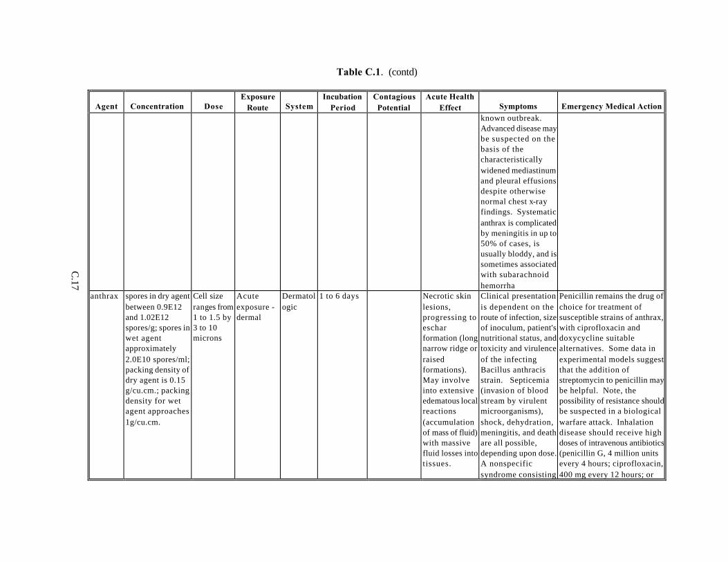
C.17

Table C.1. (contd)

Agent Concentration Dose Exposure

Route System Incubation

Period Contagious Potential

Acute Health Effect Symptoms Emergency Medical Action

known outbreak. Advanced disease may be suspected on the basis of the characteristically widened mediastinum and pleural effusions despite otherwise normal chest x-ray findings. Systematic anthrax is complicated by meningitis in up to 50% of cases, is usually bloddy, and is sometimes associated with subarachnoid hemorrha

anthrax spores in dry agent between 0.9E12 and 1.02E12 spores/g; spores in wet agent approximately 2.0E10 spores/ml; packing density of dry agent is 0.15 g/cu.cm.; packing density for wet agent approaches 1g/cu.cm.

Cell size ranges from 1 to 1.5 by 3 to 10 microns

Acute exposure - dermal

Dermatologic

1 to 6 days Necrotic skin lesions, progressing to eschar formation (long narrow ridge or raised formations). May involve into extensive edematous local reactions (accumulation of mass of fluid) with massive fluid losses into tissues.

Clinical presentation is dependent on the route of infection, size of inoculum, patient's nutritional status, and toxicity and virulence of the infecting Bacillus anthracis strain. Septicemia (invasion of blood stream by virulent microorganisms), shock, dehydration, meningitis, and death are all possible, depending upon dose. A nonspecific syndrome consisting

Penicillin remains the drug of choice for treatment of susceptible strains of anthrax, with ciprofloxacin and doxycycline suitable alternatives. Some data in experimental models suggest that the addition of streptomycin to penicillin may be helpful. Note, the possibility of resistance should be suspected in a biological warfare attack. Inhalation disease should receive high doses of intravenous antibiotics (penicillin G, 4 million units every 4 hours; ciprofloxacin, 400 mg every 12 hours; or

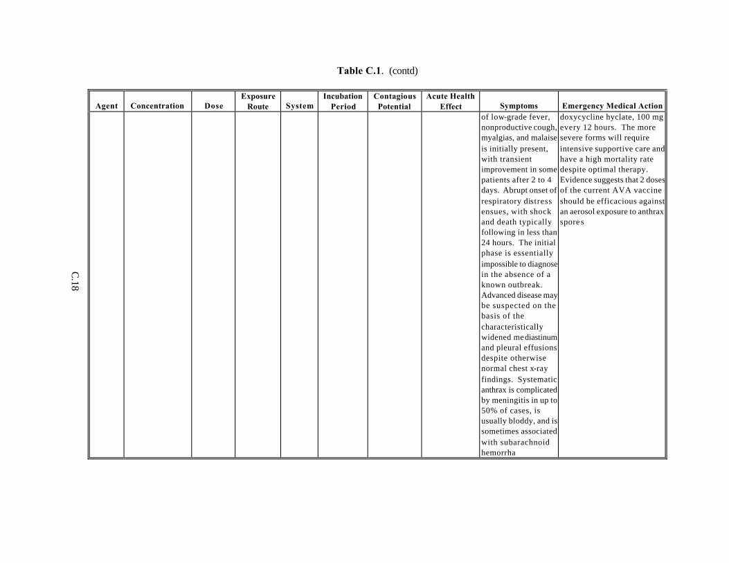
C.18

Table C.1. (contd)

Agent Concentration Dose Exposure

Route System Incubation

Period Contagious Potential

Acute Health Effect Symptoms Emergency Medical Action

of low-grade fever, nonproductive cough, myalgias, and malaise is initially present, with transient improvement in some patients after 2 to 4 days. Abrupt onset of respiratory distress ensues, with shock and death typically following in less than 24 hours. The initial phase is essentially impossible to diagnose in the absence of a known outbreak. Advanced disease may be suspected on the basis of the characteristically widened mediastinum and pleural effusions despite otherwise normal chest x-ray findings. Systematic anthrax is complicated by meningitis in up to 50% of cases, is usually bloddy, and is sometimes associated with subarachnoid hemorrha

doxycycline hyclate, 100 mg every 12 hours. The more severe forms will require intensive supportive care and have a high mortality rate despite optimal therapy. Evidence suggests that 2 doses of the current AVA vaccine should be efficacious against an aerosol exposure to anthrax spore s

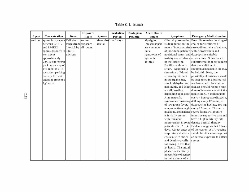
C.19

Table C.1. (contd)

Agent Concentration Dose Exposure

Route System Incubation

Period Contagious Potential

Acute Health Effect Symptoms Emergency Medical Action

anthrax spores in dry agent between 0.9E12 and 1.02E12 spores/g; spores in wet agent approximately 2.0E10 spores/ml; packing density of dry agent is 0.15 g/cu.cm.; packing density for wet agent approaches 1g/cu.cm.

Cell size ranges from 1 to 1.5 by 3 to 10 microns

Acute exposure - all routes

Musculoskeletal

1 to 6 days Myalgias (muscular pain) are common initial symptoms of systemic anthrax

Clinical presentation is dependent on the route of infection, size of inoculum, patient's nutritional status, and toxicity and virulence of the infecting Bacillus anthracis strain. Septicemia (invasion of blood stream by virulent microorganisms), shock, dehydration, meningitis, and death are all possible, depending upon dose. A nonspecific syndrome consisting of low-grade fever, nonproductive cough, myalgias, and malaise is initially present, with transient improvement in some patients after 2 to 4 days. Abrupt onset of respiratory distress ensues, with shock and death typically following in less than 24 hours. The initial phase is essentially impossible to diagnose in the absence of a

Penicillin remains the drug of choice for treatment of susceptible strains of anthrax, with ciprofloxacin and doxycycline suitable alternatives. Some data in experimental models suggest that the addition of streptomycin to penicillin may be helpful. Note, the possibility of resistance should be suspected in a biological warfare attack. Inhalation disease should receive high doses of intravenous antibiotics (penicillin G, 4 million units every 4 hours; ciprofloxacin, 400 mg every 12 hours; or doxycycline hyclate, 100 mg every 12 hours. The more severe forms will require intensive supportive care and have a high mortality rate despite optimal therapy. Evidence suggests that 2 doses of the current AVA vaccine should be efficacious against an aerosol exposure to anthrax spores

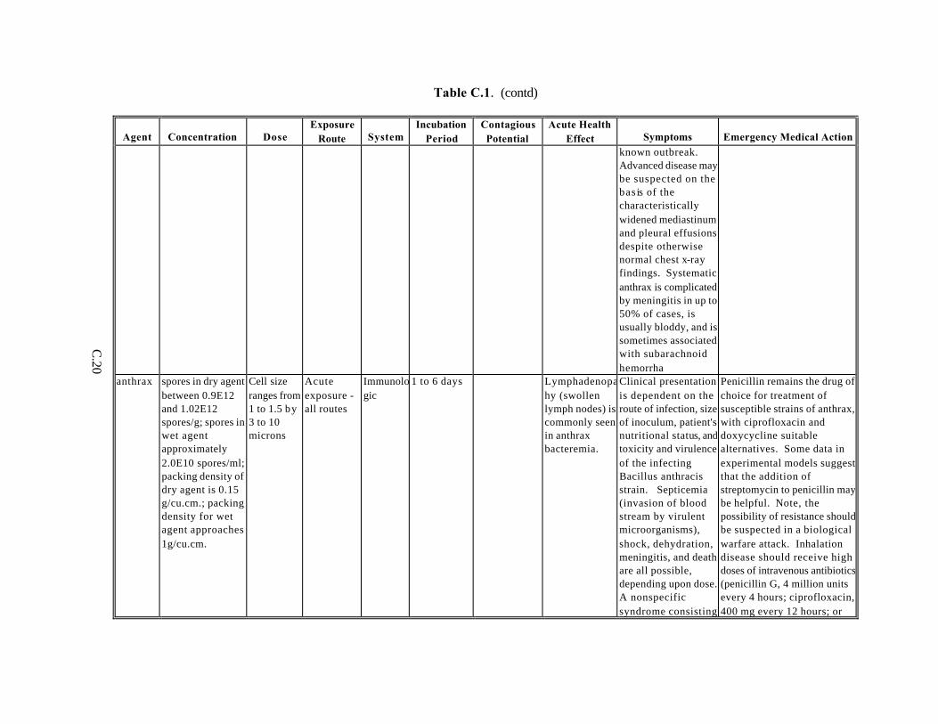
C.20

Table C.1. (contd)

Agent Concentration Dose Exposure

Route System Incubation

Period Contagious Potential

Acute Health Effect Symptoms Emergency Medical Action

known outbreak. Advanced disease may be suspected on the basis of the characteristically widened mediastinum and pleural effusions despite otherwise normal chest x-ray findings. Systematic anthrax is complicated by meningitis in up to 50% of cases, is usually bloddy, and is sometimes associated with subarachnoid hemorrha

anthrax spores in dry agent between 0.9E12 and 1.02E12 spores/g; spores in wet agent approximately 2.0E10 spores/ml; packing density of dry agent is 0.15 g/cu.cm.; packing density for wet agent approaches 1g/cu.cm.

Cell size ranges from 1 to 1.5 by 3 to 10 microns

Acute exposure - all routes

Immunologic

1 to 6 days Lymphadenopathy (swollen lymph nodes) is commonly seen in anthrax bacteremia.

Clinical presentation is dependent on the route of infection, size of inoculum, patient's nutritional status, and toxicity and virulence of the infecting Bacillus anthracis strain. Septicemia (invasion of blood stream by virulent microorganisms), shock, dehydration, meningitis, and death are all possible, depending upon dose. A nonspecific syndrome consisting

Penicillin remains the drug of choice for treatment of susceptible strains of anthrax, with ciprofloxacin and doxycycline suitable alternatives. Some data in experimental models suggest that the addition of streptomycin to penicillin may be helpful. Note, the possibility of resistance should be suspected in a biological warfare attack. Inhalation disease should receive high doses of intravenous antibiotics (penicillin G, 4 million units every 4 hours; ciprofloxacin, 400 mg every 12 hours; or

C.21

Table C.1. (contd)

Agent Concentration Dose Exposure

Route System Incubation

Period Contagious Potential

Acute Health Effect Symptoms Emergency Medical Action

of low-grade fever, nonproductive cough, myalgias, and malaise is initially present, with transient improvement in some patients after 2 to 4 days. Abrupt onset of respiratory distress ensues, with shock and death typically following in less than 24 hours. The initial phase is essentially impossible to diagnose in the absence of a known outbreak. Advanced disease may be suspected on the basis of the characteristically widened mediastinum and pleural effusions despite otherwise normal chest x-ray findings. Systematic anthrax is complicated by meningitis in up to 50% of cases, is usually bloddy, and is sometimes associated with subarachnoid hemorrha

doxycycline hyclate, 100 mg every 12 hours. The more severe forms will require intensive supportive care and have a high mortality rate despite optimal therapy. Evidence suggests that 2 doses of the current AVA vaccine should be efficacious against an aerosol exposure to anthrax spores

Appendix D

Example Chemical Health Effect Database (CHED) for Chemical Agents

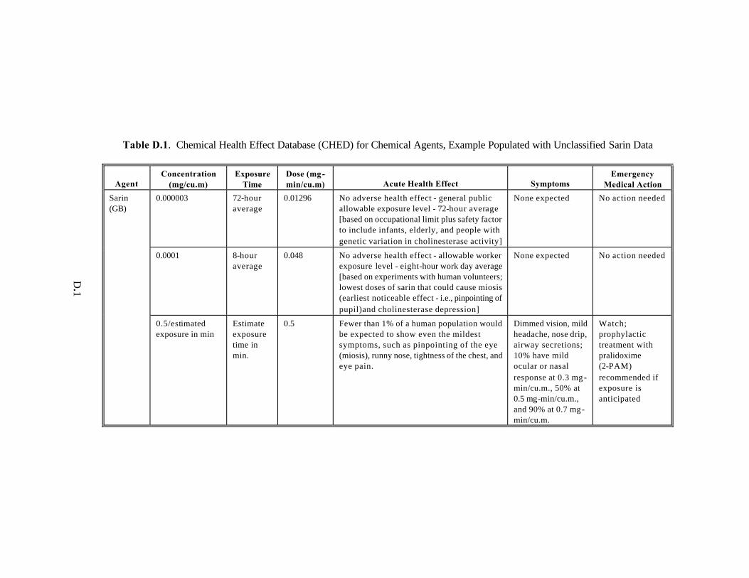
D.1

Table D.1. Chemical Health Effect Database (CHED) for Chemical Agents, Example Populated with Unclassified Sarin Data

Agent Concentration

(mg/cu.m) Exposure

Time Dose (mg-min/cu.m) Acute Health Effect Symptoms

Emergency Medical Action

Sarin (GB)

0.000003 72-hour average

0.01296 No adverse health effect - general public allowable exposure level - 72-hour average [based on occupational limit plus safety factor to include infants, elderly, and people with genetic variation in cholinesterase activity]

None expected No action needed

0.0001 8-hour average

0.048 No adverse health effect - allowable worker exposure level - eight-hour work day average [based on experiments with human volunteers; lowest doses of sarin that could cause miosis (earliest noticeable effect - i.e., pinpointing of pupil)and cholinesterase depression]

None expected No action needed

0.5/estimated exposure in min

Estimate exposure time in min.

0.5 Fewer than 1% of a human population would be expected to show even the mildest symptoms, such as pinpointing of the eye (miosis), runny nose, tightness of the chest, and eye pain.

Dimmed vision, mild headache, nose drip, airway secretions; 10% have mild ocular or nasal response at 0.3 mg -min/cu.m., 50% at 0.5 mg-min/cu.m., and 90% at 0.7 mg-min/cu.m.

Watch; prophylactic treatment with pralidoxime (2-PAM) recommended if exposure is anticipated

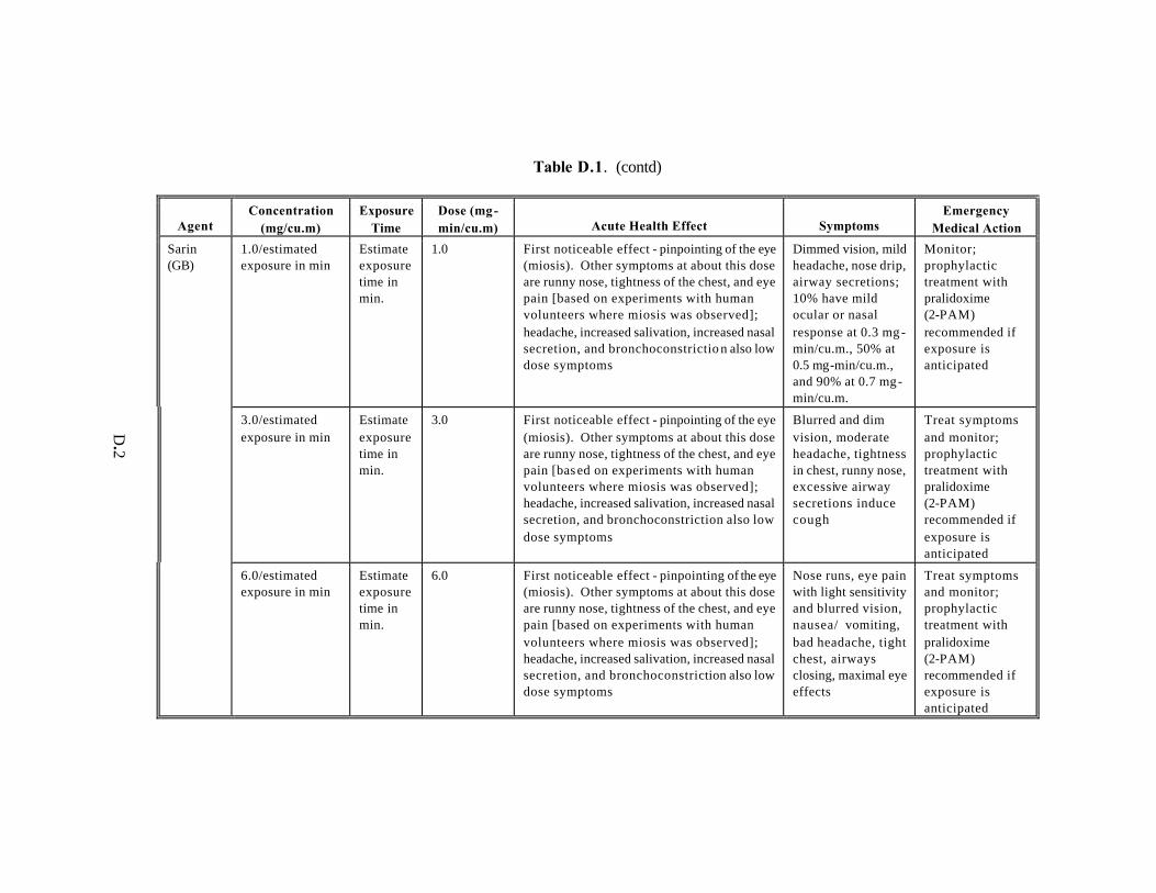
D.2

Table D.1. (contd)

Agent Concentration

(mg/cu.m) Exposure

Time Dose (mg-min/cu.m) Acute Health Effect Symptoms

Emergency Medical Action

Sarin (GB)

1.0/estimated exposure in min

Estimate exposure time in min.

1.0 First noticeable effect - pinpointing of the eye (miosis). Other symptoms at about this dose are runny nose, tightness of the chest, and eye pain [based on experiments with human volunteers where miosis was observed]; headache, increased salivation, increased nasal secretion, and bronchoconstrictio n also low dose symptoms

Dimmed vision, mild headache, nose drip, airway secretions; 10% have mild ocular or nasal response at 0.3 mg -min/cu.m., 50% at 0.5 mg-min/cu.m., and 90% at 0.7 mg-min/cu.m.

Monitor; prophylactic treatment with pralidoxime (2-PAM) recommended if exposure is anticipated

3.0/estimated exposure in min

Estimate exposure time in min.

3.0 First noticeable effect - pinpointing of the eye (miosis). Other symptoms at about this dose are runny nose, tightness of the chest, and eye pain [bas ed on experiments with human volunteers where miosis was observed]; headache, increased salivation, increased nasal secretion, and bronchoconstriction also low dose symptoms

Blurred and dim vision, moderate headache, tightness in chest, runny nose, excessive airway secretions induce cough

Treat symptoms and monitor; prophylactic treatment with pralidoxime (2-PAM) recommended if exposure is anticipated

6.0/estimated exposure in min

Estimate exposure time in min.

6.0 First noticeable effect - pinpointing of the eye (miosis). Other symptoms at about this dose are runny nose, tightness of the chest, and eye pain [based on experiments with human volunteers where miosis was observed]; headache, increased salivation, increased nasal secretion, and bronchoconstriction also low dose symptoms

Nose runs, eye pain with light sensitivity and blurred vision, nausea/ vomiting, bad headache, tight chest, airways closing, maximal eye effects

Treat symptoms and monitor; prophylactic treatment with pralidoxime (2-PAM) recommended if exposure is anticipated

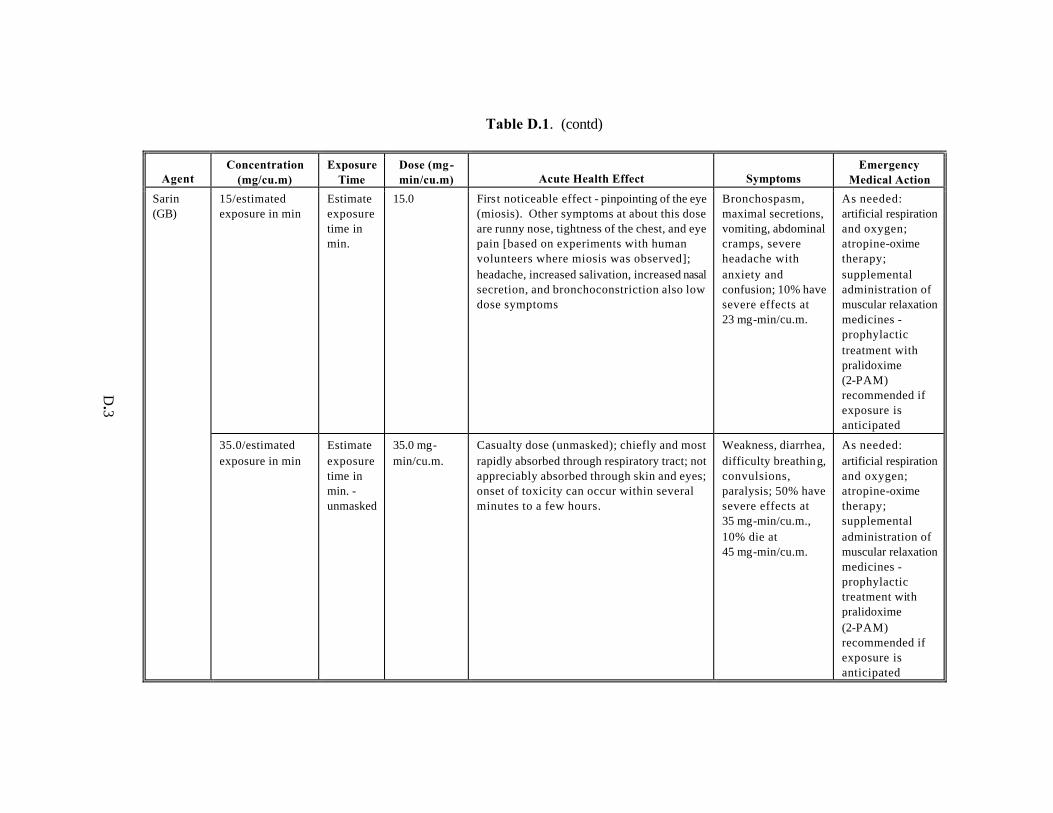
D.3

Table D.1. (contd)

Agent Concentration

(mg/cu.m) Exposure

Time Dose (mg-min/cu.m) Acute Health Effect Symptoms

Emergency Medical Action

Sarin (GB)

15/estimated exposure in min

Estimate exposure time in min.

15.0 First noticeable effect - pinpointing of the eye (miosis). Other symptoms at about this dose are runny nose, tightness of the chest, and eye pain [based on experiments with human volunteers where miosis was observed]; headache, increased salivation, increased nasal secretion, and bronchoconstriction also low dose symptoms

Bronchospasm, maximal secretions, vomiting, abdominal cramps, severe headache with anxiety and confusion; 10% have severe effects at 23 mg-min/cu.m.

As needed: artificial respiration and oxygen; atropine-oxime therapy; supplemental administration of muscular relaxation medicines - prophylactic treatment with pralidoxime (2-PAM) recommended if exposure is anticipated

35.0/estimated exposure in min

Estimate exposure time in min. - unmasked

35.0 mg-min/cu.m.

Casualty dose (unmasked); chiefly and most rapidly absorbed through respiratory tract; not appreciably absorbed through skin and eyes; onset of toxicity can occur within several minutes to a few hours.

Weakness, diarrhea, difficulty breathing, convulsions, paralysis; 50% have severe effects at 35 mg-min/cu.m., 10% die at 45 mg-min/cu.m.

As needed: artificial respiration and oxygen; atropine-oxime therapy; supplemental administration of muscular relaxation medicines - prophylactic treatment with pralidoxime (2-PAM) recommended if exposure is anticipated

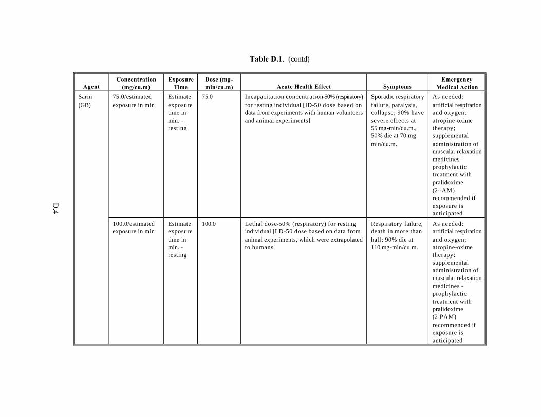
D.4

Table D.1. (contd)

Agent Concentration

(mg/cu.m) Exposure

Time Dose (mg-min/cu.m) Acute Health Effect Symptoms

Emergency Medical Action

75.0/estimated exposure in min

Estimate exposure time in min. - resting

75.0 Incapacitation concentration-50% (respiratory) for resting individual [ID-50 dose based on data from experiments with human volunteers and animal experiments]

Sporadic respiratory failure, paralysis, collapse; 90% have severe effects at 55 mg-min/cu.m., 50% die at 70 mg-min/cu.m.

As needed: artificial respiration and oxygen; atropine-oxime therapy; supplemental administration of muscular relaxation medicines - prophylactic treatment with pralidoxime (2--AM) recommended if exposure is anticipated

Sarin (GB)

100.0/estimated exposure in min

Estimate exposure time in min. -resting

100.0 Lethal dose-50% (respiratory) for resting individual [LD-50 dose based on data from animal experiments, which were extrapolated to humans]

Respiratory failure, death in more than half; 90% die at 110 mg-min/cu.m.

As needed: artificial respiration and oxygen; atropine-oxime therapy; supplemental administration of muscular relaxation medicines - prophylactic treatment with pralidoxime (2-PAM) recommended if exposure is anticipated