Indicator Constraints in Mixed-Integer Programming · Andrea Lodi University of Bologna, Italy -...
47
Indicator Constraints in Mixed-Integer Programming Andrea Lodi University of Bologna, Italy - [email protected] Amaya Nogales-Gómez, Universidad de Sevilla, Spain Pietro Belotti, FICO, UK Matteo Fischetti, Michele Monaci, Domenico Salvagnin, University of Padova, Italy Pierre Bonami, IBM, Spain SCIP Workshop 2014 @ Berlin (Germany), October 2, 2014 1
Transcript of Indicator Constraints in Mixed-Integer Programming · Andrea Lodi University of Bologna, Italy -...

Indicator Constraintsin Mixed-Integer Programming
Andrea LodiUniversity of Bologna, Italy - [email protected]
Amaya Nogales-Gómez, Universidad de Sevilla, Spain
Pietro Belotti, FICO, UK
Matteo Fischetti, Michele Monaci, Domenico Salvagnin, University of Padova, Italy
Pierre Bonami, IBM, Spain
SCIP Workshop 2014 @ Berlin (Germany), October 2, 2014
1
Introduction Deactivating Linear Constraints
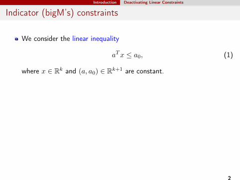
Indicator (bigM’s) constraints
We consider the linear inequality
aTx ≤ a0, (1)
where x ∈ Rk and (a, a0) ∈ Rk+1 are constant.
It is a well-known modeling trick in Mixed-Integer Linear Programming(MILP) to use a binary variable y multiplied by a sufficiently big(positive) constant M in order to deactivate constraint (1)
aTx ≤ a0 +My. (2)
It is also well known the risk of such a modeling trick, namelyweak Linear Programming (LP) relaxations, andnumerical issues.
2

Introduction Deactivating Linear Constraints
Indicator (bigM’s) constraints
We consider the linear inequality
aTx ≤ a0, (1)
where x ∈ Rk and (a, a0) ∈ Rk+1 are constant.It is a well-known modeling trick in Mixed-Integer Linear Programming(MILP) to use a binary variable y multiplied by a sufficiently big(positive) constant M in order to deactivate constraint (1)
aTx ≤ a0 +My. (2)
It is also well known the risk of such a modeling trick, namelyweak Linear Programming (LP) relaxations, andnumerical issues.
2
Introduction Deactivating Linear Constraints
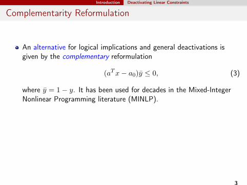
Complementarity Reformulation
An alternative for logical implications and general deactivations isgiven by the complementary reformulation
(aTx− a0)y ≤ 0, (3)
where y = 1− y. It has been used for decades in the Mixed-IntegerNonlinear Programming literature (MINLP).
The obvious drawback of the above reformulation is its nonconvexity.Thus, the complementary reformulation has been used so far if (andonly if) the problem at hand was already nonconvex, as it is often thecase, for example, in Chemical Engineering applications.
3

Introduction Deactivating Linear Constraints
Our goal
In this talk we argue against this common rule of always pursuing alinear reformulation for logical implications.
We do that by exposing a class of Mixed-Integer Convex QuadraticProgramming (MIQP) problems arising in Supervised Classificationwhere the Global Optimization (GO) solver Couenne usingreformulation (3) is out-of-the-box consistently faster than virtuallyany state-of-the-art commercial MIQP solver like IBM-Cplex, Gurobiand Xpress.
This is quite counter-intuitive because, in general, convex MIQPsadmit more efficient solution techniques both in theory and inpractice, especially because they benefit of virtually all machinery ofMILP solvers.
4

A class of surprising problems Supervised Classification
Support Vector Machine (SVM)
5

A class of surprising problems Supervised Classification
The input data
Ω: the population.Population is partitioned into two classes, −1,+1.For each object in Ω, we have
x = (x1, . . . , xd) ∈ X ⊂ Rd: predictor variables.y ∈ −1,+1: class membership.
The goal is to find a hyperplane ω>x+ b = 0 that aims at separating,if possible, the two classes.Future objects will be classified as
y = +1 if ω>x+ b > 0
y = −1 if ω>x+ b < 0 (4)
6

A class of surprising problems Supervised Classification
Soft-margin approach
minω>ω
2+
n∑i=1
g(ξi)
subject to
yi(ω>xi + b) ≥ 1− ξi i = 1, . . . , n
ξi ≥ 0 i = 1, . . . , n
ω ∈ Rd, b ∈ R
where n is the size of the population and g(ξi) = Cn ξi the most popular
choice for the loss function.
7
A class of surprising problems Supervised Classification
Ramp Loss Model (Brooks, OR, 2011)
Ramp Loss Function g(ξi) = (minξi, 2)+ yielding the Ψ-learningapproach, with (a)+ = maxa, 0.
minω>ω
2+C
n(
n∑i=1
ξi+2n∑
i=1
zi)
s.t. (RLM)
yi(ω>xi + b) ≥ 1− ξi−Mzi ∀i = 1, . . . , n
0 ≤ ξi≤ 2 ∀i = 1, . . . , n
z ∈ 0, 1nω ∈ Rd, b ∈ R
with M > 0 big enough constant.
8

A class of surprising problems Supervised Classification
Ramp Loss Model (Brooks, OR, 2011)
Ramp Loss Function g(ξi) = (minξi, 2)+ yielding the Ψ-learningapproach, with (a)+ = maxa, 0.
minω>ω
2+C
n(
n∑i=1
ξi+2
n∑i=1
zi)
s.t. (RLM)
yi(ω>xi + b) ≥ 1− ξi−Mzi ∀i = 1, . . . , n
0 ≤ ξi≤ 2 ∀i = 1, . . . , n
z ∈ 0, 1nω ∈ Rd, b ∈ R
with M > 0 big enough constant.
8

A class of surprising problems Raw Computational Results
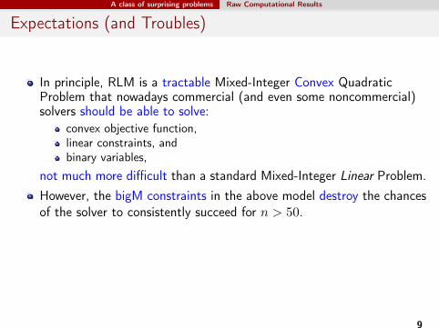
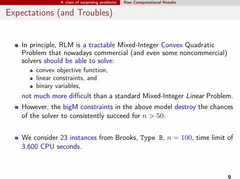
Expectations (and Troubles)
In principle, RLM is a tractable Mixed-Integer Convex QuadraticProblem that nowadays commercial (and even some noncommercial)solvers should be able to solve:
convex objective function,linear constraints, andbinary variables,
not much more difficult than a standard Mixed-Integer Linear Problem.
However, the bigM constraints in the above model destroy the chancesof the solver to consistently succeed for n > 50.
We consider 23 instances from Brooks, Type B, n = 100, time limit of3,600 CPU seconds.
9
A class of surprising problems Raw Computational Results
Expectations (and Troubles)
In principle, RLM is a tractable Mixed-Integer Convex QuadraticProblem that nowadays commercial (and even some noncommercial)solvers should be able to solve:
convex objective function,linear constraints, andbinary variables,
not much more difficult than a standard Mixed-Integer Linear Problem.However, the bigM constraints in the above model destroy the chancesof the solver to consistently succeed for n > 50.
We consider 23 instances from Brooks, Type B, n = 100, time limit of3,600 CPU seconds.
9

A class of surprising problems Raw Computational Results
Solving the MIQP by IBM-Cplex
23 instances from Brooks,Type B, n = 100,time limit of 3,600 CPU seconds.
IBM-Cplex is able to find theoptimal solution (%gap of theupper bound, ub) BUT
it fails to improve thecontinuous relaxation byterminating after 1h with a large%gap for the lower bound, lb.
3 A Raw Set of Computational Results
We have tested the nonconvex MINLP formulation proposed in Section 2 on allartificial datasets proposed by Brooks [3]. However, in this section we concentrateon a subset of them (23 instances of size n = 100, Type B, see [3] for details)showing the surprising behavior that Couenne out-of-the-box performs betterthan IBM-Cplex. Table 1 reports the straightforward comparison. Computingtimes (time) in CPU seconds, number of nodes (nodes), percentage gap of theupper (ub) and lower (lb) bounds are reported, as well as the optimal value ofeach instance for future reference. A time limit of 1 hour is provided to each runand in case such a limit is reached the entry in the column “time” indicates a“tl”. For instances solved to optimality gaps are reported as “–”.
Table 1. Computational results for Couenne and IBM-Cplex. Instances of Type B [3],n = 100, time limit of 1 hour.
Couenne IBM-Cplex
% gap % gapoptimal value time (sec.) nodes ub lb time (sec.) nodes ub lb
1 157,995.00 163.61 17,131 – – 3,438.49 16,142,440 – –2 179,368.00 1,475.68 181,200 – – tl 12,841,549 – 23.613 220,674.00 tl 610,069 14.96 15.38 tl 20,070,294 – 37.824 5,225.99 160.85 25,946 – – tl 20,809,936 – 9.375 5,957.08 717.20 131,878 – – tl 17,105,372 – 26.176 11,409,600.00 1,855.16 221,618 – – tl 13,865,833 – 22.677 11,409,100.00 482.19 56,710 – – tl 14,619,065 – 21.408 10,737,700.00 491.26 55,292 – – tl 13,347,313 – 14.599 5,705,360.00 1,819.42 216,831 – – tl 12,257,994 – 22.22
10 5,704,800.00 807.95 89,894 – – tl 13,054,400 – 23.1311 5,369,020.00 536.40 62,291 – – tl 14,805,943 – 12.3712 2,853,240.00 1,618.79 196,711 – – tl 12,777,936 – 21.9713 2,852,680.00 630.18 83,676 – – tl 14,075,300 – 23.3214 2,684,660.00 533.77 65,219 – – tl 13,994,099 – 12.4815 1,427,170.00 2,007.62 211,157 – – tl 10,671,225 – 23.0816 1,426,620.00 641.05 72,617 – – tl 12,984,857 – 22.7217 1,342,480.00 728.93 73,142 – – tl 12,564,000 – 14.1118 714,142.00 1,784.93 193,286 – – tl 11,217,844 – 23.4519 713,583.00 752.50 84,538 – – tl 12,854,704 – 22.7220 671,396.00 412.16 48,847 – – tl 14,018,831 – 12.4321 357,626.00 2,012.62 223,702 – – tl 11,727,308 – 23.5522 357,067.00 768.73 104,773 – – tl 15,482,162 – 18.6723 335,852.00 706.39 70,941 – – tl 12,258,164 – 14.88
The results of Table 1 are quite straightforward to interpret, with a strictdominance of Couenne with respect to IBM-Cplex. In the unique instance Couenneis unable to solve to optimality (instance 3) the issue is probably that the upperbound is not improved enough, thus being unable to propagate (see next sec-tion) and strengthen the formulation. Conversely, IBM-Cplex is always able tofind the right upper bound (namely, the optimal solution value) but the lowerbound value remains far from the optimal value, thus being unable to proveoptimality.
Due to space reasons, we reported in Table 1 detailed numbers only forIBM-Cplex but we solved the convex MIQP model (4)–(9) with the convex MIQPsolvers developed extending the three major MILP solvers, namely Gurobi andXpress, and IBM-Cplex itself. The three solvers behave very similarly in theconsidered instances, thus indicating that the weakness shown in Table 1 is
10

A class of surprising problems Raw Computational Results
Reformulating by Complementarity
minω>ω
2+C
n
(n∑
i=1
ξi+2
n∑i=1
(1− zi))
(yi(ω>xi + b)− 1 + ξi)·zi ≥ 0 ∀i = 1, . . . , n
0 ≤ ξi ≤ 2 ∀i = 1, . . . , n
z ∈ 0, 1nω ∈ Rd
b ∈ R,
where zi = 1− zi, andthe resulting model is a Mixed-Integer Nonconvex QuadraticallyConstrained Problem (MIQCP) that IBM-Cplex, like all othercommercial solvers initially developed for MILP, cannot solve (yet).
11

A class of surprising problems Raw Computational Results
Solving the MIQCP by Couenne
Despite thenonconvexity ofthe aboveMIQCP, there areseveral options torun the newmodel as it is andone of them isthe open-sourcesolver Couennebelonging to theCoin-OR arsenal.
3 A Raw Set of Computational Results
We have tested the nonconvex MINLP formulation proposed in Section 2 on allartificial datasets proposed by Brooks [3]. However, in this section we concentrateon a subset of them (23 instances of size n = 100, Type B, see [3] for details)showing the surprising behavior that Couenne out-of-the-box performs betterthan IBM-Cplex. Table 1 reports the straightforward comparison. Computingtimes (time) in CPU seconds, number of nodes (nodes), percentage gap of theupper (ub) and lower (lb) bounds are reported, as well as the optimal value ofeach instance for future reference. A time limit of 1 hour is provided to each runand in case such a limit is reached the entry in the column “time” indicates a“tl”. For instances solved to optimality gaps are reported as “–”.
Table 1. Computational results for Couenne and IBM-Cplex. Instances of Type B [3],n = 100, time limit of 1 hour.
Couenne IBM-Cplex
% gap % gapoptimal value time (sec.) nodes ub lb time (sec.) nodes ub lb
1 157,995.00 163.61 17,131 – – 3,438.49 16,142,440 – –2 179,368.00 1,475.68 181,200 – – tl 12,841,549 – 23.613 220,674.00 tl 610,069 14.96 15.38 tl 20,070,294 – 37.824 5,225.99 160.85 25,946 – – tl 20,809,936 – 9.375 5,957.08 717.20 131,878 – – tl 17,105,372 – 26.176 11,409,600.00 1,855.16 221,618 – – tl 13,865,833 – 22.677 11,409,100.00 482.19 56,710 – – tl 14,619,065 – 21.408 10,737,700.00 491.26 55,292 – – tl 13,347,313 – 14.599 5,705,360.00 1,819.42 216,831 – – tl 12,257,994 – 22.22
10 5,704,800.00 807.95 89,894 – – tl 13,054,400 – 23.1311 5,369,020.00 536.40 62,291 – – tl 14,805,943 – 12.3712 2,853,240.00 1,618.79 196,711 – – tl 12,777,936 – 21.9713 2,852,680.00 630.18 83,676 – – tl 14,075,300 – 23.3214 2,684,660.00 533.77 65,219 – – tl 13,994,099 – 12.4815 1,427,170.00 2,007.62 211,157 – – tl 10,671,225 – 23.0816 1,426,620.00 641.05 72,617 – – tl 12,984,857 – 22.7217 1,342,480.00 728.93 73,142 – – tl 12,564,000 – 14.1118 714,142.00 1,784.93 193,286 – – tl 11,217,844 – 23.4519 713,583.00 752.50 84,538 – – tl 12,854,704 – 22.7220 671,396.00 412.16 48,847 – – tl 14,018,831 – 12.4321 357,626.00 2,012.62 223,702 – – tl 11,727,308 – 23.5522 357,067.00 768.73 104,773 – – tl 15,482,162 – 18.6723 335,852.00 706.39 70,941 – – tl 12,258,164 – 14.88
The results of Table 1 are quite straightforward to interpret, with a strictdominance of Couenne with respect to IBM-Cplex. In the unique instance Couenneis unable to solve to optimality (instance 3) the issue is probably that the upperbound is not improved enough, thus being unable to propagate (see next sec-tion) and strengthen the formulation. Conversely, IBM-Cplex is always able tofind the right upper bound (namely, the optimal solution value) but the lowerbound value remains far from the optimal value, thus being unable to proveoptimality.
Due to space reasons, we reported in Table 1 detailed numbers only forIBM-Cplex but we solved the convex MIQP model (4)–(9) with the convex MIQPsolvers developed extending the three major MILP solvers, namely Gurobi andXpress, and IBM-Cplex itself. The three solvers behave very similarly in theconsidered instances, thus indicating that the weakness shown in Table 1 is
12

Interpreting the numbers Why are the results surprising?
What does Couenne do?
Although,Convex MIQP should be much easier than nonconvex MIQCP, andIBM-Cplex is by far more sophisticated than Couenne
one can still argue that a comparison in performance between twodifferent solution methods and computer codes is anyway hard toperform.
However, the reported results are rather surprising, especially if onedigs into the way in which Couenne solves the problem, namelyconsidering three aspects:
1 McCormick Linearization,2 Branching, and3 alternative L1 norm.
13
Interpreting the numbers Why are the results surprising?
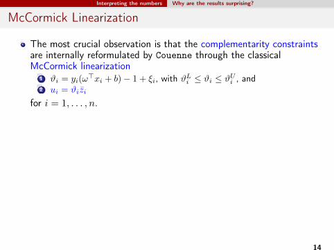
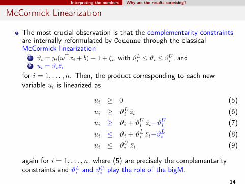
McCormick Linearization
The most crucial observation is that the complementarity constraintsare internally reformulated by Couenne through the classicalMcCormick linearization
1 ϑi = yi(ω>xi + b)− 1 + ξi, with ϑLi ≤ ϑi ≤ ϑUi , and
2 ui = ϑizi
for i = 1, . . . , n.
Then, the product corresponding to each newvariable ui is linearized as
ui ≥ 0 (5)ui ≥ ϑLi zi (6)ui ≥ ϑi + ϑUi zi−ϑUi (7)ui ≤ ϑi + ϑLi zi−ϑLi (8)ui ≤ ϑUi zi (9)
again for i = 1, . . . , n, where (5) are precisely the complementarityconstraints and ϑLi and ϑUi play the role of the bigM.
14
Interpreting the numbers Why are the results surprising?
McCormick Linearization
The most crucial observation is that the complementarity constraintsare internally reformulated by Couenne through the classicalMcCormick linearization
1 ϑi = yi(ω>xi + b)− 1 + ξi, with ϑLi ≤ ϑi ≤ ϑUi , and
2 ui = ϑizi
for i = 1, . . . , n. Then, the product corresponding to each newvariable ui is linearized as
ui ≥ 0 (5)ui ≥ ϑLi zi (6)ui ≥ ϑi + ϑUi zi−ϑUi (7)ui ≤ ϑi + ϑLi zi−ϑLi (8)ui ≤ ϑUi zi (9)
again for i = 1, . . . , n, where (5) are precisely the complementarityconstraints and ϑLi and ϑUi play the role of the bigM.
14

Interpreting the numbers Why are the results surprising?
Branching
It is well known that a major component of GO solvers is the iterativetightening of the convex (most of the time linear) relaxation of thenonconvex feasible region by branching on continuous variables.
However, the default version of Couenne does not take advantage ofthis possibility and branches (first) on binary variables z’s.
Thus, again it is surprising that such a branching strategy leads to animprovement over the sophisticated branching framework ofIBM-Cplex.
15
Interpreting the numbers Why are the results surprising?
Alternative L1 norm
A natural question is if the reported results are due to the somehowless sophisticated evolution of MILP solvers in their MIQP extensionswith respect to the MILP one.
In order to answer this question we performed an experiment in whichthe quadratic part of the objective function has been replaced by itsL1 norm making the entire bigM model linear. Ultimately, theabsolute value of ω is minimized.
Computationally, this has no effect and Couenne continues toconsistently outperform MILP solvers on this very special (modified)class of problems.
16

Interpreting the numbers Bound Reduction in nonconvex MINLPs
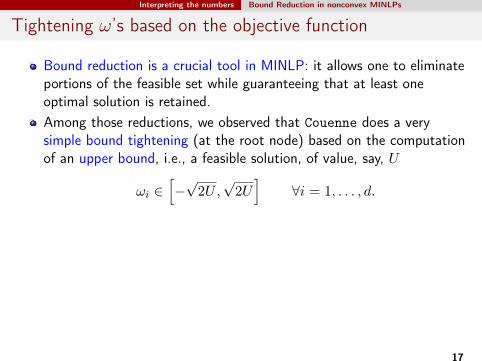
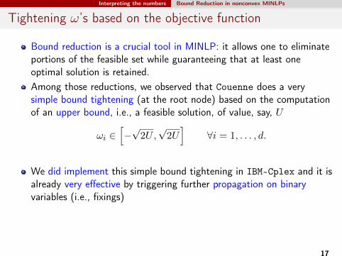
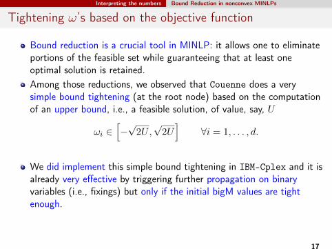
Tightening ω’s based on the objective function
Bound reduction is a crucial tool in MINLP: it allows one to eliminateportions of the feasible set while guaranteeing that at least oneoptimal solution is retained.
Among those reductions, we observed that Couenne does a verysimple bound tightening (at the root node) based on the computationof an upper bound, i.e., a feasible solution, of value, say, U
ωi ∈[−√
2U,√
2U]
∀i = 1, . . . , d.
We did implement this simple bound tightening in IBM-Cplex and it isalready very effective by triggering further propagation on binaryvariables (i.e., fixings) but only if the initial bigM values are tightenough.In other words, when the bigM values are large it is very hard to solvethe problem without changing them during search.
17
Interpreting the numbers Bound Reduction in nonconvex MINLPs
Tightening ω’s based on the objective function
Bound reduction is a crucial tool in MINLP: it allows one to eliminateportions of the feasible set while guaranteeing that at least oneoptimal solution is retained.Among those reductions, we observed that Couenne does a verysimple bound tightening (at the root node) based on the computationof an upper bound, i.e., a feasible solution, of value, say, U
ωi ∈[−√
2U,√
2U]
∀i = 1, . . . , d.
We did implement this simple bound tightening in IBM-Cplex and it isalready very effective by triggering further propagation on binaryvariables (i.e., fixings)
but only if the initial bigM values are tightenough.In other words, when the bigM values are large it is very hard to solvethe problem without changing them during search.
17
Interpreting the numbers Bound Reduction in nonconvex MINLPs
Tightening ω’s based on the objective function
Bound reduction is a crucial tool in MINLP: it allows one to eliminateportions of the feasible set while guaranteeing that at least oneoptimal solution is retained.Among those reductions, we observed that Couenne does a verysimple bound tightening (at the root node) based on the computationof an upper bound, i.e., a feasible solution, of value, say, U
ωi ∈[−√
2U,√
2U]
∀i = 1, . . . , d.
We did implement this simple bound tightening in IBM-Cplex and it isalready very effective by triggering further propagation on binaryvariables (i.e., fixings) but only if the initial bigM values are tightenough.
In other words, when the bigM values are large it is very hard to solvethe problem without changing them during search.
17
Interpreting the numbers Bound Reduction in nonconvex MINLPs
Tightening ω’s based on the objective function
Bound reduction is a crucial tool in MINLP: it allows one to eliminateportions of the feasible set while guaranteeing that at least oneoptimal solution is retained.Among those reductions, we observed that Couenne does a verysimple bound tightening (at the root node) based on the computationof an upper bound, i.e., a feasible solution, of value, say, U
ωi ∈[−√
2U,√
2U]
∀i = 1, . . . , d.
We did implement this simple bound tightening in IBM-Cplex and it isalready very effective by triggering further propagation on binaryvariables (i.e., fixings) but only if the initial bigM values are tightenough.In other words, when the bigM values are large it is very hard to solvethe problem without changing them during search.
17
Interpreting the numbers Bound Reduction in nonconvex MINLPs
Much more sophisticated propagation
It has to be noted that Couenne internal bigM values (namely ϑLi andϑUi ) are much more conservative (and safe) than those used in theSVM literature.
Nevertheless, the sophisticated bound reduction loop implemented byGO solvers does the job. Iteratively,
new feasible solutions propagate on the ω variables,that leads to strengthen MC constraints (by changing the ϑi bounds),that in turn propagates on binary variables.Conversely, branching on the zieither (zi = 0) increases the lower bound,thus triggering additional ω tightening,or (zi = 1) tightens the bounds on ϑi, thuspropagating again on ω.
Switching off in Couenne any of these components leads to a dramaticdegradation in the results.
18

Interpreting the numbers Bound Reduction in nonconvex MINLPs
Much more sophisticated propagation
It has to be noted that Couenne internal bigM values (namely ϑLi andϑUi ) are much more conservative (and safe) than those used in theSVM literature.Nevertheless, the sophisticated bound reduction loop implemented byGO solvers does the job.
Iteratively,new feasible solutions propagate on the ω variables,that leads to strengthen MC constraints (by changing the ϑi bounds),that in turn propagates on binary variables.Conversely, branching on the zieither (zi = 0) increases the lower bound,thus triggering additional ω tightening,or (zi = 1) tightens the bounds on ϑi, thuspropagating again on ω.
Switching off in Couenne any of these components leads to a dramaticdegradation in the results.
18

Interpreting the numbers Bound Reduction in nonconvex MINLPs
Much more sophisticated propagation
It has to be noted that Couenne internal bigM values (namely ϑLi andϑUi ) are much more conservative (and safe) than those used in theSVM literature.Nevertheless, the sophisticated bound reduction loop implemented byGO solvers does the job. Iteratively,
new feasible solutions propagate on the ω variables,that leads to strengthen MC constraints (by changing the ϑi bounds),that in turn propagates on binary variables.
Conversely, branching on the zieither (zi = 0) increases the lower bound,thus triggering additional ω tightening,or (zi = 1) tightens the bounds on ϑi, thuspropagating again on ω.
Switching off in Couenne any of these components leads to a dramaticdegradation in the results.
18

Interpreting the numbers Bound Reduction in nonconvex MINLPs
Much more sophisticated propagation
It has to be noted that Couenne internal bigM values (namely ϑLi andϑUi ) are much more conservative (and safe) than those used in theSVM literature.Nevertheless, the sophisticated bound reduction loop implemented byGO solvers does the job. Iteratively,
new feasible solutions propagate on the ω variables,that leads to strengthen MC constraints (by changing the ϑi bounds),that in turn propagates on binary variables.Conversely, branching on the zieither (zi = 0) increases the lower bound,thus triggering additional ω tightening,or (zi = 1) tightens the bounds on ϑi, thuspropagating again on ω.
Switching off in Couenne any of these components leads to a dramaticdegradation in the results.
18

Interpreting the numbers Bound Reduction in nonconvex MINLPs
Much more sophisticated propagation
It has to be noted that Couenne internal bigM values (namely ϑLi andϑUi ) are much more conservative (and safe) than those used in theSVM literature.Nevertheless, the sophisticated bound reduction loop implemented byGO solvers does the job. Iteratively,
new feasible solutions propagate on the ω variables,that leads to strengthen MC constraints (by changing the ϑi bounds),that in turn propagates on binary variables.Conversely, branching on the zieither (zi = 0) increases the lower bound,thus triggering additional ω tightening,or (zi = 1) tightens the bounds on ϑi, thuspropagating again on ω.
Switching off in Couenne any of these components leads to a dramaticdegradation in the results.
18

With a little help of my friends Bound tightening by enumeration
Initial Bound tightening
Bound reduction at the root node can make use of enumeration.
Iterative domain reductionwhile (hope_to_improve) do
for each i ∈ [1, d] doli = minωi : (w, ξ, zi) ∈ P,Z(w, ξ, zi) ≤ Uui = maxωi : (w, ξ, zi) ∈ P,Z(w, ξ, zi) ≤ U
where:- P is the set of feasible solutions (including bound constraints),- Z(w, ξ, zi) is the cost of solution (w, ξ, zi), and- U is the value of an upper bound.
The MILPs need not to be solved to optimality: li and ui are thebounds returned by the MIP within a node limit.Improve lower and upper bounds for ωi variables → possibly fix someωi and/or zi variables.
19
With a little help of my friends Bound tightening by enumeration
Initial Bound tightening
Bound reduction at the root node can make use of enumeration.Iterative domain reduction
while (hope_to_improve) dofor each i ∈ [1, d] doli = minωi : (w, ξ, zi) ∈ P,Z(w, ξ, zi) ≤ Uui = maxωi : (w, ξ, zi) ∈ P,Z(w, ξ, zi) ≤ U
where:- P is the set of feasible solutions (including bound constraints),- Z(w, ξ, zi) is the cost of solution (w, ξ, zi), and- U is the value of an upper bound.
The MILPs need not to be solved to optimality: li and ui are thebounds returned by the MIP within a node limit.Improve lower and upper bounds for ωi variables → possibly fix someωi and/or zi variables.
19

With a little help of my friends Bound tightening by enumeration
Iterated domain reduction
Iterate domain reduction can be seen as a preprocessing tool.The better the initial solution U , the more effective the reduction.It can be time consuming, but dramatically improves the results:
Use IBM-Cplex for 100k nodes (+ 10 polish nodes) to compute theinitial solution U .Use IBM-Cplex for 100k nodes for each lower/upper bound tightening.All instances with d = 2 solved to optimality:
average CPU time ' 30 secondsaverage # of nodes: 412k
Iterating the process allows IBM-Cplex’s internal preprocessing toolsto propagate the current domain of the variables.
20

With a little help of my friends Bound tightening and bigM reduction
IBM-Cplex work in progress
3 A Raw Set of Computational Results
We have tested the nonconvex MINLP formulation proposed in Section 2 on allartificial datasets proposed by Brooks [?]. However, in this section we concentrateon a subset of them (23 instances of size n = 100, Type B, see [?] for details)showing the surprising behavior that Couenne out-of-the-box performs betterthan IBM-Cplex. Table 1 reports the straightforward comparison. Computingtimes (time) in CPU seconds, number of nodes (nodes), percentage gap of theupper (ub) and lower (lb) bounds are reported, as well as the optimal value ofeach instance for future reference. A time limit of 1 hour is provided to each runand in case such a limit is reached the entry in the column “time” indicates a“tl”. For instances solved to optimality gaps are reported as “–”.
Table 1. Computational results for Couenne and IBM-Cplex. Instances of Type B [?],n = 100, time limit of 1 hour.
CPLEX 12.6.0 CPLEX w.i.p.optimal value time time time ratio
1 157,995.00 6799.8 253.8 0.042 179,368.00 10000.0 3467.2 0.353 220,674.00 10000.0 10000.0 1.004 5,225.99 10000.0 314.8 0.035 5,957.08 10000.0 10000.0 1.006 11,409,600.00 10000.0 7995.7 0.807 11,409,100.00 10000.0 521.9 0.058 10,737,700.00 10000.0 2300.0 0.239 5,705,360.00 10000.0 10000.0 1.00
10 5,704,800.00 10000.0 1015.0 0.1011 5,369,020.00 10000.0 10000.0 1.0012 2,853,240.00 10000.0 10000.0 1.0013 2,852,680.00 10000.0 871.4 0.0914 2,684,660.00 10000.0 2552.6 0.2615 1,427,170.00 10000.0 10000.0 1.0016 1,426,620.00 10000.0 2656.3 0.2717 1,342,480.00 10000.0 10000.0 1.0018 714,142.00 10000.0 3841.2 0.3819 713,583.00 10000.0 942.3 0.0920 671,396.00 10000.0 8653.7 0.8721 357,626.00 10000.0 2608.0 0.2622 357,067.00 10000.0 1094.2 0.1123 335,852.00 10000.0 10000.0 1.00
The results of Table 1 are quite straightforward to interpret, with a strictdominance of Couenne with respect to IBM-Cplex. In the unique instance Couenneis unable to solve to optimality (instance 3) the issue is probably that the upperbound is not improved enough, thus being unable to propagate (see next sec-tion) and strengthen the formulation. Conversely, IBM-Cplex is always able tofind the right upper bound (namely, the optimal solution value) but the lowerbound value remains far from the optimal value, thus being unable to proveoptimality.
Due to space reasons, we reported in Table 1 detailed numbers only forIBM-Cplex but we solved the convex MIQP model (4)–(9) with the convex MIQPsolvers developed extending the three major MILP solvers, namely Gurobi andXpress, and IBM-Cplex itself. The three solvers behave very similarly in theconsidered instances, thus indicating that the weakness shown in Table 1 isstructurally associated with solving the big-M formulation, or, conversely, thatsolving the nonconvex formulation through a GO solver is e↵ective.
21
Conclusions
In a broad sense, we have used the SVM with the ramp loss toinvestigate the possibility of exploiting tools from (nonconvex) MINLPin MILP or (convex) MIQP, essentially, the reverse of the commonpath.
More precisely, we have argued that sophisticated (nonconvex) MINLPtools might be very effective to face one of the most structural issuesof MILP, which is dealing with the weak continuous relaxationsassociated with bigM constraints.
We have shown that the crucial bound reduction can be obtained apriori, in this special case by solving MILPs on the weak bigMformulation.
More generally, a full integration of such a bound reduction tool forindicator constraints can be obtained by local cuts.
22

Disclaimer
IBM’s statements regarding its plans, directions, and intent are subject tochange or withdrawal without notice at IBM’s sole discretion. Informationregarding potential future products is intended to outline our generalproduct direction and it should not be relied on in making a purchasingdecision. The information mentioned regarding potential future products isnot a commitment, promise, or legal obligation to deliver any material,code or functionality. Information about potential future products may notbe incorporated into any contract. The development, release, and timing ofany future features or functionality described for our products remains atour sole discretion. Performance is based on measurements and projectionsusing standard IBM benchmarks in a controlled environment. The actualthroughput or performance that any user will experience will varydepending upon many factors, including considerations such as the amountof multiprogramming in the user’s job stream, the I/O configuration, thestorage configuration, and the workload processed. Therefore, no assurancecan be given that an individual user will achieve results similar to thosestated here.
23
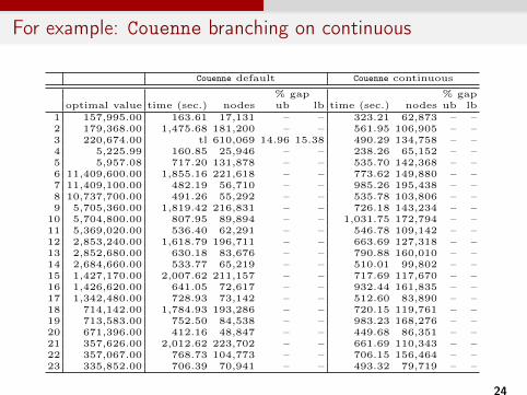
For example: Couenne branching on continuous
5.4 Even better: Branching on Continuous Variables
As anticipated in Section 4, even better performance for Couenne could beobtained by branching on continuous variables. Namely, instructed to branchpreferably on continuous Couenne always selects # variables, which clearly leadto additional bound tightening with respect to branch on binaries. Indeed, if ina given relaxation we have #i = c, the two branches #i c OR #i c propagateas follows: (i) if c < 0 then #i c implies zi = 0 OR (ii) if c > 0 then #i cimplies zi = 1. This is in addition to the already discussed bidirectional boundtightening of ! and b. The results are reported in Table 2 and clearly show thecomputational advantage of this choice.
Table 2. Computational results for Couenne default and Couenne branching emphasison continuous variables. Instances of Type B [3], n = 100, time limit of 1 hour.
Couenne default Couenne continuous
% gap % gapoptimal value time (sec.) nodes ub lb time (sec.) nodes ub lb
1 157,995.00 163.61 17,131 – – 323.21 62,873 – –2 179,368.00 1,475.68 181,200 – – 561.95 106,905 – –3 220,674.00 tl 610,069 14.96 15.38 490.29 134,758 – –4 5,225.99 160.85 25,946 – – 238.26 65,152 – –5 5,957.08 717.20 131,878 – – 535.70 142,368 – –6 11,409,600.00 1,855.16 221,618 – – 773.62 149,880 – –7 11,409,100.00 482.19 56,710 – – 985.26 195,438 – –8 10,737,700.00 491.26 55,292 – – 535.78 103,806 – –9 5,705,360.00 1,819.42 216,831 – – 726.18 143,234 – –
10 5,704,800.00 807.95 89,894 – – 1,031.75 172,794 – –11 5,369,020.00 536.40 62,291 – – 546.78 109,142 – –12 2,853,240.00 1,618.79 196,711 – – 663.69 127,318 – –13 2,852,680.00 630.18 83,676 – – 790.88 160,010 – –14 2,684,660.00 533.77 65,219 – – 510.01 99,802 – –15 1,427,170.00 2,007.62 211,157 – – 717.69 117,670 – –16 1,426,620.00 641.05 72,617 – – 932.44 161,835 – –17 1,342,480.00 728.93 73,142 – – 512.60 83,890 – –18 714,142.00 1,784.93 193,286 – – 720.15 119,761 – –19 713,583.00 752.50 84,538 – – 983.23 168,276 – –20 671,396.00 412.16 48,847 – – 449.68 86,351 – –21 357,626.00 2,012.62 223,702 – – 661.69 110,343 – –22 357,067.00 768.73 104,773 – – 706.15 156,464 – –23 335,852.00 706.39 70,941 – – 493.32 79,719 – –
6 Conclusions
We have shown that the nonconvex reformulation of so-called big-M constraintsand the consequent use of a general-purpose MINLP solver instead of a MIQPsolver can lead, surprisingly, to faster computing times for a special class of clas-sification problems. Through a careful analysis of Couenne features and compo-nents we have been able to isolate those that make a di↵erence, namely aggressivebound tightening and iterative strengthening of the McCormick linearization. Itis conceivable that similar reformulations tightened in the same way can be ef-fective for other problems involving logical implications and disjunctions of thistype.
The biggest challenge at the moment is to export these techniques, or better,their more extensive use, in solvers like IBM-Cplex. The current attempts in theform of cut generators strengthening the big-M values of formulation (4)–(9),
24