Index numbers and their relationship with the economy
154
ECLAC Methodologies Index numbers and their relationship with the economy Federico Dorin Daniel Perrotti Patricia Goldszier
Transcript of Index numbers and their relationship with the economy

ECLAC Methodologies
Inde
x nu
mbe
rs a
nd th
eir r
elat
ions
hip
wit
h th
e ec
onom
yN
o. 1
Index numbers and their relationship with the economy
Federico Dorin Daniel Perrotti
Patricia Goldszier

ECLACPublications
Thank you for your interest in
this ECLAC publication
Please register if you would like to receive information on our editorial
products and activities. When you register, you may specify your particular
areas of interest and you will gain access to our products in other formats.
www.cepal.org/en/publications
Publicaciones www.cepal.org/apps

Alicia BárcenaExecutive Secretary
Mario CimoliDeputy Executive Secretary
Raúl García-BuchacaDeputy Executive Secretary for Management and Programme Analysis
Rolando OcampoChief, Statistics Division
Ricardo PérezChief, Publications and Web Services Division
This publication was prepared by Federico Dorin, Daniel Perrotti and Patricia Goldszier under the auspices of the Statistics Division of the Economic Commission for Latin America and the Caribbean (ECLAC) and the ECLAC office in Washington, D.C.
The authors are grateful to Salvador Marconi and Mara Riestra for their detailed reading of the document and valuable comments, and to Pascual Gerstenfeld, Inés Bustillo and Giovanni Savio for their support for its preparation.
The views expressed in this document are those of the authors and do not necessarily reflect the views of the Organization.
United Nations publicationISBN: 978-92-1-122038-4 (print)ISBN: 978-92-1-004737-1 (pdf)ISBN: 978-92-1-358272-5 (ePub)Sales No.: E.18.II.G.13LC/PUB.2018/12-PDistribution: GCopyright © United Nations, 2020All rights reservedPrinted at United Nations, SantiagoS.19-01059
This publication should be cited as: F. Dorin, D. Perrotti and P. Goldszier, Index numbers and their relationship with the economy, ECLAC Methodologies, No. 1 (LC/PUB.2018/12-P), Santiago, Economic Commission for Latin America and the Caribbean (ECLAC), 2020.
Applications for authorization to reproduce this work in whole or in part should be sent to the Economic Commission for Latin America and the Caribbean (ECLAC), Publications and Web Services Division, [email protected]. Member States and their governmental institutions may reproduce this work without prior authorization, but are requested to mention the source and to inform ECLAC of such reproduction.

Contents
Introduction ................................................................................................................11
Chapter I Direct comparison and choice of an index from the consumer’s standpoint ............ 13A. Averages approach ............................................................................................14
1. Simple or elementary indices .....................................................................142. Complex indices ......................................................................................... 15
B. Fixed-basket approach ...................................................................................... 241. Laspeyres price index ................................................................................ 252. Paasche price index ................................................................................... 263. Laspeyres price index and type of mean .................................................... 274. Paasche price index and type of mean ...................................................... 28
C. Axiomatic approach .......................................................................................... 32D. Stochastic approach ......................................................................................... 34E. Economic approach .......................................................................................... 36
1. The “real” cost of living index...................................................................... 372. Choice of a consumption basket ................................................................ 40
Chapter II Direct comparison and the producer perspective ................................................... 53
Chapter III Indirect comparison and chain-linked indices .......................................................... 61A. Indirect comparison ........................................................................................... 61B. Chain-linked indices .......................................................................................... 63
Chapter IV Purchasing power parity .......................................................................................... 69A. Law of one price ................................................................................................ 70B. What is purchasing power parity? ....................................................................... 71C. What are PPPs used for? ................................................................................... 73D. Comparing international prices ......................................................................... 73
1. Creation of the baskets of goods and services .......................................... 742. Collection and validation of price data ....................................................... 753. Collection and validation of data for weighting .......................................... 754. Estimating purchasing power parity .......................................................... 76
E. International comparison of volumes over time ................................................. 88F. International Comparison Program ................................................................... 89
1. Presentation of the Program and background ........................................... 892. Information requirements ......................................................................... 903. The prices .................................................................................................. 914. The weights ............................................................................................... 925. Other components of GDP ......................................................................... 93
G. Results of the 2011 round of the International Comparison Program .................. 95
Bibliography .............................................................................................................101

4 Economic Commission for Latin America and the Caribbean (ECLAC)Contents
Annexes................................................................................................................... 107
Annex A1 ...................................................................................................................109Annex A2 ................................................................................................................... 111Annex A3 ...................................................................................................................113
Stage 1: Cost minimization at initial prices ........................................................113Stage 2: Cost minimization at updated prices ...................................................114Stage 3: Estimating the cost of living ................................................................115
Annex A4 ...................................................................................................................1161. Definitionofthefunction ...........................................................................1162. Budget constraint .....................................................................................1173. Maximizing production: direct and indirect production function ................1174. Minimization of production costs ..............................................................1205. Elasticity of substitution between factors ................................................ 123
Annex A5 .................................................................................................................. 126Annex A6 .................................................................................................................. 127Annex A7 .................................................................................................................. 136
Exercise 1: Calculation of PPP for a basic heading ............................................ 136Exercise 2: Aggregation of two basic headings ................................................144
Annex A8 .................................................................................................................. 1461. Quaranta tables ........................................................................................ 1462. Dikhanov tables ........................................................................................1483. Reference parities ....................................................................................150
Tables
I.1 Hypothetical prices of wine and bread for an exercise to calculate the general price level................................................................... 13
I.2 Application of the elementary price index formula to the wine and bread example........................................................................................... 15
I.3 Calculation of the price level using the simple arithmetic mean ....................... 16I.4 Calculation of the price level using the simple harmonic mean ........................ 17I.5 Calculation of the price level using the simple geometric mean ....................... 17I.6 Verificationofthechange-of-unitproperty ..................................................... 18I.7 Verificationofpassage-of-timeproperty .........................................................19I.8 Price indices and percentage changes of simple arithmetic,
harmonic and geometric means ......................................................................19I.9 Calculating the value of the basket with a price of wine that doubles
and a price of bread that halves ...................................................................... 20I.10 Weights ...........................................................................................................21I.11 Alternative mean and weighting combinations ................................................21I.12 Formulae for the alternative of mean and weighting combinations ................. 22I.13 Formulae for the various mean and weighting combinations,
expressed in terms of elementary price indices .............................................. 22I.14 Rates of change in the general price level from 2013 to 2014 (equal weights) ........ 23I.15 Rates of change in the general price level from 2013 to 2014 (variable weights) .... 23I.16 Data from the example of wine and bread prices with handpicked quantities ....... 25I.17 Fleetwood Price Index (arithmetic mean with 2013 prices
and handpicked quantities) ............................................................................. 25

5Index numbers and their relationship with the economy Contents
I.18 Laspeyres price index and its percentage change .......................................... 26I.19 Paasche price index and its percentage change ............................................. 27I.20 Indices for the alternatives combinations of mean and weighting ................... 28I.21 Fisher price index (geometric mean of Laspeyres and Paasche indices) ........... 29I.22 Törnqvist price index (geometric mean of the geometric
Laspeyres and Paasche indices) ..................................................................... 29I.23 Walsh price index ............................................................................................. 31I.24 Basic and additional criteria applicable to the indices,
accordingtothefirstaxiomaticapproach ...................................................... 32I.25 Axioms applicable to the indices, according to the second
axiomatic approach ....................................................................................... 36I.26 Data of the exercise ........................................................................................ 42I.27 Cost of living index according to different price index formulas ...................... 46I.28 Exact price indices for different cost-of-living indices derived
from utility functions ...................................................................................... 46I.29 Results of the main price indices for selected utility functions ....................... 46II.1 Initial situation ................................................................................................ 55II.2 Successive unit increases in the factor K ........................................................ 55II.3 Doubling of factors K and L ............................................................................. 56III.1 Prices used in the indirect comparison exercise, 2013-2017 ............................. 61III.2 Quantities used in the indirect comparison exercise, 2013-2017 ....................... 61III.3 Fisher price index ........................................................................................... 62III.4 Change of base year in each new year ............................................................. 63III.5 Fisher price indices with base years 2013, 2014, 2015, 2016 and 2017 ............... 64III.6 Annual rates of variation in the Fisher price index ........................................... 64III.7 Chain-linked Fisher price index with reference period 2013 = 1 ........................ 65III.8 Selected countries: formulas used to calculate consumer price indices ......... 66III.9 Selected countries: formulas used to measure gross
domestic product (GDP) volume indices .......................................................... 67IV.1 Product data for basic heading 1 ......................................................................77IV.2 Example of the structure of the basket of goods and services
used in the International Comparison Program for the individual household consumption component ............................................................... 91
IV.3 Latin America and the Caribbean and selected countries of the Organization for Economic Cooperation and Development (OECD): individual household consumption expenditure, according to the International Comparison Program, 2011 ......................................................... 97
IV.4 Latin America and the Caribbean and selected countries of the Organization for Economic Cooperation and Development (OECD): gross domestic product, International Comparison Program, 2011 .................. 99
A1.1 Variable prices and quantities ........................................................................109A1.2 Weighted arithmetic price index, 2013 ...........................................................109A1.3 Weighted arithmetic price index, 2014 ...........................................................109A1.4 Weighted harmonic price index, 2013 .............................................................109A1.5 Weighted harmonic price index, 2014 ............................................................. 110A1.6 Weighted geometric price index, 2013 ........................................................... 110A1.7 Weighted geometric price index, 2014 ........................................................... 110

6 Economic Commission for Latin America and the Caribbean (ECLAC)Contents
A2.1 Variable prices and quantities ......................................................................... 111A2.2 Weighted arithmetic price index, 2013 ............................................................ 111A2.3 Weighted arithmetic price index, 2014 ............................................................ 111A2.4 Weighted harmonic price index, 2013 .............................................................. 111A2.5 Weighted harmonic price index, 2014 ..............................................................112A2.6 Weighted geometric price index, 2013 ............................................................112A2.7 Weighted geometric price index, 2014 ............................................................112A5.1 Frequency of chaining and problem of “drift” in the case
ofpriceandquantityfluctuations .................................................................. 126A6.1 Gross value added by sector and GDP............................................................. 127A6.2 Gross value added by sector and GDP............................................................. 127A6.3 Elementary volume indices ............................................................................ 128A6.4 Annual weights at current prices ................................................................... 129A6.5 Elementary volume indices ............................................................................ 129A6.6 Links ..............................................................................................................130A6.7 Chain-linked index and GDP as a chain-volume measure
in monetary terms referenced to 2005 ...........................................................130A6.8 GDP at constant 2005 prices and statistical discrepancy due
to non-additivity .............................................................................................131A6.9 Gross domestic product by expenditure component ...................................... 132A6.10 Gross domestic product by expenditure component ...................................... 132A6.11 Chain-linked volume index (reference year: 2005) and GDP
as a chain-volume measure in monetary terms referenced to 2005, measured on the expenditure side ................................................................. 133
A6.12 Gross value added by sector, with further breakdown and gross domestic product (GDP) ................................................................................. 134
A6.13 Gross value added by sector, with further disaggregation, GDP ..................... 134A6.14 Chain-linked volume index (reference year: 2005) and GDP
according to the 2005 monetary chain, with further breakdown, from the production approach ....................................................................... 135
A7.1 Price matrix ................................................................................................... 136A7.2 Country A as a base ....................................................................................... 136A7.3 Country B as a base ....................................................................................... 137A7.4 Country C as a base ....................................................................................... 138A7.5 Country D as a base ....................................................................................... 138A7.6 Summary of the purchasing power parity of a basic heading ......................... 139A7.7 Transitivity ..................................................................................................... 139A7.8 Price matrix ...................................................................................................140A7.9 Country A as base ..........................................................................................140A7.10 Country B as base ...........................................................................................141A7.11 Country C as base ...........................................................................................141A7.12 Country D as a base .......................................................................................142A7.13 Summary of the non-transitive purchasing power parity
of a basic heading .......................................................................................... 143A7.14 Non-transitive ............................................................................................... 143A7.15 Purchasing power parity. Jevons-GEKS ........................................................ 143A7.16 Parity matrix ..................................................................................................144

7Index numbers and their relationship with the economy Contents
A7.17 Expenditure matrix ........................................................................................144A7.18 Calculation of Laspeyres indices using the base country expenditure ................144A7.19 Calculation of the Paasche indices ................................................................144A7.20 Calculation of Fisher indices .......................................................................... 145A7.21 Application of the Jevons-GEKS method ....................................................... 145A7.22 Transitivity ..................................................................................................... 145A7.23 Change of base .............................................................................................. 145A8.1 Quaranta table ............................................................................................... 146A8.2 Dikhanov table ...............................................................................................148A8.3 Table..............................................................................................................150
Figures
I.1 Lagrange multiplier – graphical solution ......................................................... 43I.2 New situation: increase in the price of product Qx .......................................... 44I.3 Graphical representation of the new unobservable basket ............................. 44I.4 Functions with homothetic preferences .......................................................... 51I.5 Functions with non-homothetic preferences .................................................. 52
Boxes
I.1 Hicksian substitution and income effects ...................................................... 45I.2 Homothetic utility functions and cost of living index ....................................... 50III.1 Basechange:fixed-baseorchain-linked ....................................................... 68IV.1 The Big Mac Index ........................................................................................... 72A4.1 Roy’s identity .................................................................................................120A4.2 Shephard’s Lemma ........................................................................................ 123


Symbols and abbreviations
α CommoninflationrateB0 Minimum expenditure to maximize utilityσ Elasticity of substitutionεi Independently distributed random variables, with mean 0 and variance σ2
gt Geometric meanht Harmonic meanI IncomeCLIt Cost of living indexCIt-x,t Chained-linked index of t referenced to period t-xGLIt Geometric Laspeyres indexGPIt Geometric Paasche indexDPIt Drobisch price indexelPI Elementary price indexFlPIt Fleetwood price indexFPIt Fisher price indexGYPIt Geometric Young price indexLMPIt Lloyd-Moulton price indexLoPIt Lowe price indexLPIt Laspeyres price indexPPIt Paasche price indexQMrt Quadratic-mean-of-order-r price indexThPIt Theil price indexTPIt Tornqvist price indexWPIt Walsh price indexYPIt Young price indexPIt Basic price indexIt-1,t Index of t referenced to prices in period in t-1mt Arithmetic mean in period tN Number of observationsPt Price of the good in period tpi Probability, expected valueQh Hicksian or compensated demandQ Quantity of “handpicked” good iQm Marshallian demandQ Quantity of good i in period tQ * Quantity of goods that in time t produce a utility equal to that of t-1ri ri= ln (p0
i / wti) values taken by a discrete random variable, R
Vt Utility level in period tw Weighting of good i in period tX Variable i at time t


Introduction
Index numbers are the basic tool for synthesizing economic statistics, to enable the formulae used to express and describe variables such as a country’s economic growth or an economy’s inflationrate,andalsotomakeinternationalcomparisons.Ifdifferentformulaeare used, the results vary, and comparisons are not valid; so it is important to understand the formulae being used. Moreover, countries and international organizations need to promote common practices that harmonize and standardize measurements.
Although index numbers are associated with macroeconomics, their theoretical foundation lies in microeconomics. The recommended practices and microeconomic theoretical underpinning are disseminated in manuals compiled by various international agencies, including the United Nations Statistics Division, the International Monetary Fund (IMF),theWorldBank,theInternationalLabourOrganization(ILO),theStatisticalOfficeof the European Union (Eurostat) and the Organization for Economic Cooperation and Development (OECD).
This publication summarizes the links between price and volume indices and microeconomic theory; and it presents the formulae that are recommended for international measurements, and explains how to use them in international price and volume comparisons.


Chapter IDirect comparison1 and choice of an index from the consumer’s standpoint
Imagine an economy that has just two products (wine and bread), with prices in two periods (2013 and 2014) as shown in table I.1. From 2013 to 2014, the price of wine doubles (from US$ 20toUS$ 40),andthepriceofbreadhalves(fromUS$ 20toUS$ 10).Thequestionis:how much does the general price level vary from one year to the other?
■ Table I.1 Hypothetical prices of wine and bread for an exercise to calculate the general price level
YearPrice of wine(dollars/litre)
Price of bread(dollars/kg)
General price level
2013 20 20?
2014 40 10
Source: Prepared by the authors.
The geneice level is a type of “index number”, a “price index” (PI)2whichshouldreflectthe general movement of prices in the economy.
1 Direct, bilateral or binary indices compare two periods directly, while ignoring intermediate periods. The comparison can be made between consecutive periods, for example, one year and the next (or the previous year), or between periods that are further apart in time.
2 The other types of index number are quantity or volume indices and value indices (the latter take account of both price and volume changes). Spatial indices are also compiled to compare prices of the same product in different regions or countries; these make it possible to calculate currency purchasing power parities and are discussed in chapter IV of this document. Lastly, relative price indices are compiled to compare prices of different products.

14 Economic Commission for Latin America and the Caribbean (ECLAC)Chapter I
In this example, there are theoretically three possible answers to the question: (i) a rise in the general price level between 2013 and 2014; (ii) a fall in the general price level; or (iii)nochange.Sinceastatisticalofficecannotgivethreeanswerstothesamequestion,theory and practice need to be considered, along with the epistemological elements of the discipline, to provide a single solution.
Logical reasoning can also be applied: if the prices of the goods are known in two periods, and the price of one of the goods doubles but the other price halves, the aggregate price level should be the same in both periods, so that the overall price change would be 0%.
Whetherthisfirstapproximationsurvivesscrutinyfromotherscientificperspectives,such as statistics or economics, will be considered below. In doing so, answers are sought usingtheaveragesapproachandthoseproposedinILOandothers(2006),thefixed-basketapproach, the axiomatic (or test) approach, the stochastic approach and the economic approach. This initial analysis uses the consumer’s perspective, while chapter II approaches the problem from the producer’s standpoint.
A. Averages approach
The averages approach, as its name implies, consists of applying an average to prices or price indices to obtain a general measure of the price or index in question. Before considering this definition,adistinctionshouldbemadebetweensimpleorelementaryindicesandcomplexindices.
1. Simple or elementary indices
Apriceindexthatisdefinedforanindividualproductisreferredtoassimpleorelementaryprice index (elPI), because it applies to a single product.3 Its formula is: 4
where:
: elementary price index in period t, referenced to the price5 in period 0
Pt : price of the good in period t
P0 : price of the good in period 0
3 The “single product” concept means a homogeneous product. At the macroeconomic level, international productclassifiers(suchastheCentralProductClassification–CPC)groupdifferentproductclassesunderone category. This makes it impossible to rigorously estimate an elementary index for a country, since it will always group different classes of products under a single heading. In the example used in this study, bread or wine encompass different classes of such products, with different qualities, characteristics, and prices. However, in these cases the “elementary index” concept is maintained.
4 This elementary price index formula is also called the “price relative”.5 The term “base price” refers to the period against which the other prices are compared, in this case period 0.
See the distinction between the “base price”, the “base weighting” and the “base index” in chapter III.

15Index numbers and their relationship with the economy Chapter I
Applying the elementary price index formula to the example in table I.1 gives the result shown in table I.2.
■ Table I.2 Application of the elementary price index formula to the wine and bread example
YearPrice of wine(dollars/litre)
Price of bread(dollars/kg)
Wine price index(base 100=2013)
Bread price index(base 100=2013)
2013 20 20 100 100
2014 40 10 200 50
Source: Prepared by the authors.
Thus,theelementarypriceindexforwineis100in2013and200in2014.Thisreflectsthe fact that the price doubled between those two periods (the price per litre went from US$ 20toUS$ 40).Incontrast,theindexforbreadwas100in2013buthadfallento50in2014,sincethepriceperkilogramhalvedfromUS$ 20toUS$ 10.
2. Complex indices
If, instead of calculating elementary price (or quantity) indices, the aim is to compile an aggregate index that considers the behaviour of prices as a whole, or the general level of prices (or quantities), the problem of aggregation arises: how should heterogeneous products such as wine and bread be added together?
In the example, the price of wine doubles between 2013 and 2014 and the price of bread halves. This is a simple example, since the basket contains only two goods. However, the initial question again arises: what happens to the general price index of the basket of goods, does it rise, fall, or stay the same? The price index is no longer elementary or simple but complex: it is composed of two or more prices.
Theproblemcouldbesolvedbycalculatinganaveragewhich:(i)isweighted;(ii) allowsseveralobservationstobeconflatedintoasinglevalue;and(iii)reflectsatypicalstandardthat is comparable at different times.
However, the calculation is complicated by two selection problems: (i) the choice of the average (one type of average must be selected from among the many that exist); and (ii) thechoiceofweight(theweightingperiodmustbeselected—theinitialperiod(2013),thefinalperiod(2014)orsomeother.
(a) Choice of the average
The most common averages are the mean, which can be arithmetic, harmonic, or geometric; the median,6 which is the central value in a set of numbers ordered by size; and the mode,7 which is the value that occurs most frequently.
6 For the data set {2, 2, 3, 6, 8, 10, 15], the median is 6.7 From the same data set, the mode is 2.

16 Economic Commission for Latin America and the Caribbean (ECLAC)Chapter I
Use of the median and mode is ruled out, as they are less sophisticated averages than the mean and, generally, are seldom used. Returning to the example, the general price level is calculated below by applying each of the three types of mean.
(i) Simple arithmetic mean
This is expressed by the following formula:
where:
mt : arithmetic mean in period t
: variable representing the good i to be averaged (price, quantity or other measurement) at time t
N : number of observations
Applying the arithmetic mean to the prices of wine and bread gives the result shown in table I.3.
■ Table I.3 Calculation of the price level using the simple arithmetic mean
YearPrice of wine(dollars/litre)
Price of bread(dollars/kg)
Arithmetic mean Price index, arithmetic mean
Percentage variation in price level
2013 20 20 20 100 -
2014 40 10 25 125 25
Source: Prepared by the authors.
Thus, according to the arithmetic mean, the price index of the basket containing wine and bread rises by 25% between 2013 and 2014.
(ii) Simple harmonic mean
The formula in this case is:
This is calculated using the following procedure. First the arithmetic mean of the inverses of the X values is calculated:
Then the inverse of that operation is obtained, and the result is multiplied by 100. Applying the formula to the bread and wine example gives the result shown in table I.4.

17Index numbers and their relationship with the economy Chapter I
■ Table I.4 Calculation of the price level using the simple harmonic mean
Year1/Price of wine
(dollars/litre)1/Price of bread
(dollars/kg)
Arithmetic mean
(dollars)
Inverse of the average
Price index, harmonic
mean
Percentage change in price
level
2013 0.05 0.05 0.05 20 100 -
2014 0.025 0.1 0.0625 16 80 -20
Source: Prepared by the authors.
As the table shows, the general price level calculated using the harmonic mean reports the opposite trend to that obtained with the arithmetic mean. While the price index calculated with arithmetic mean reports an increase, when the harmonic is used it registers a decrease. The harmonic-mean price index follows the price that falls. In the example, the price of bread falls, and the general price index tends to follow the evolution of the price that becomes lower and lower. The opposite occurs with the arithmetic mean, for which the general price level follows the rising price (in this case the wine).
(iii) Simple geometric mean
The formula for the geometric mean consists of the nth root of the product of the N values:
Applying this to the example gives the results shown in table I.5.
■ Table I.5 Calculation of the price level using the simple geometric mean
YearPrice of wine(dollars/litre)
Price of bread(dollars/kg)
Geometric mean Price index, geometric mean
Percentage change in price level
2013 20 20 20 100 -
2014 40 10 20 100 0
Source: Prepared by the authors.
This results in a 0% change in the price level. This index is generally used for the purpose of averaging rates of change.
(b) Choosing the best mean
When trying to obtain a general index of the price level of a basket consisting of two products, three different answers were obtained: with the arithmetic mean, the general price level rises; with the harmonic mean, it falls; and, with the geometric mean, it does not vary. Which of the three is the “true” rate of variation of the general price level? To see whethertheseresultsarejustified,itisnecessarytoexaminetwopropertiesorstatisticaltests: (i) change of unit; and (ii) passage of time.

18 Economic Commission for Latin America and the Caribbean (ECLAC)Chapter I
(i) Change of unit8
The change-of-unit property states that the price index does not change if the units in which the products are measured are changed.
In the example, multiplying the price of wine each year by 100 gives the results shown in table I.6.
■ Table I.6 Verification of the change-of-unit property
YearPrice of
wine(dollars/litre)
Price of bread(dollars/kg)
Arithmetic mean
Price index,
arithmetic mean
Harmonic mean
Price index,
harmonic mean
Geometric mean
Price index,
geometric mean
2013 2 000 20 1010 100 39.6039 100 200 100
2014 4 000 10 2005 198.51 19.9501 50.37 200 100
Source: Prepared by the authors.
Thetableshowsthatonlythegeometricmeansatisfiesthechange-of-unitproperty.The arithmetic mean follows the extreme high value (wine), since the index reports a higher rate of variation than that calculated in table I.3 (98.51% compared to 25%, respectively). The harmonic mean tracks the extreme low value (the bread), since the index registers a higher rate of variation (in absolute-value terms) than that of table I.4 (-49.6% compared to -20%).
(ii) Passage of time
According to this property, the rise or fall in the general price level should not be affected by the passage of time.
In the example, the price variation repeats itself every year: the price of wine doubles and the price of bread halves. At the elementary level, the behaviour of prices is the same each year (the price of wine doubles and the price of bread halves). However, the variation in the general price level varies from year to year using either the arithmetic mean and the harmonic average. This is not the case in the geometric mean, where the aggregate rate of variationforallyearsis0%.Onlythegeometricmeansatisfiesthepassage-of-timeproperty.
The analysis can also be extended to additional periods, repeating the year-on-year price changes, that is assuming that the price of wine doubles and the price of bread halves every year, as shown in table I.7.
8 This test is the “commensurability criterion” (test 10 in the axiomatic approach discussed in section C).

19Index numbers and their relationship with the economy Chapter I
■ Table I.7 Verification of passage-of-time property
YearPrice of wine
(dollars)Price of bread
(dollars)Wine price index(base 2003=100)
Bread price index(base 2003=100)
2013 20 20 100 100.00
2014 40 10 200 50.00
2015 80 5 400 25.00
2016 160 2.5 800 12.50
2017 320 1.25 1 600 6.25
2018 640 0.625 3 200 3.13
2019 1 280 0.313 6 400 1.56
2020 2 560 0.156 12 800 0.78
2021 5 120 0.078 25 600 0.39
2022 10 240 0.039 51 200 0.20
2023 20 480 0.020 102 400 0.10
Source: Prepared by the authors.
Applying the three types of mean produces the results shown in table I.8.
■ Table I.8 Price indices and percentage changes of simple arithmetic, harmonic and geometric means
Year
Price index, arithmetic
mean(base
2003=100)
Percentage variation in price level, arithmetic
mean
Price index, harmonic
mean(base
2003=100)
Percentage variation in price level,
harmonic mean
Price index, geometric
mean(base
2003=100)
Percentage variation in price level, geometric
mean
2013 100.00 - 100.00 - 100.00 -
2014 125.00 25 80.00 -20.00 100.00 0
2015 212.50 70 47.06 -41.18 100.00 0
2016 406.25 91.18 24.62 -47.69 100.00 0
2017 803.13 97.69 12.45 -49.42 100.00 0
2018 1 601.56 99.42 6.24 -49.85 100.00 0
2019 3 200.78 99.85 3.12 -49.96 100.00 0
2010 6 400.39 99.96 1.56 -49.99 100.00 0
2011 12 800.20 99.99 0.78 -50.00 100.00 0
2012 25 600.10 100.00 0.39 -50.00 100.00 0
2013 51 200.05 100.00 0.20 -50.00 100.00 0
Source: Prepared by the authors.
The variations in the general price level obtained with the arithmetic mean are positive every year, with trend that increases each year before stabilizing at 100%, and they are biased by the extreme high values, in this case, the price of the product for which the price rises (wine).

20 Economic Commission for Latin America and the Caribbean (ECLAC)Chapter I
Variations in the general price level calculated using the harmonic mean are negative every year, with an increasing trend until they stabilize around -50%. They are biased by the extreme low values, in this case, the price of the product whose price decreases (bread).
The variation in the general price level estimated with the geometric mean is 0% in all periods, which shows that it is not biased by extreme values, whether high or low.
Insummary,sincethegeometricmeanistheonlyonethatsatisfiesthetwopropertiesin question (change of unit and passage of time), it can be considered as the mean that gives an optimal result, or “true” value. The “correct” rate of change in the example is 0%, which is consistent with the logical reasoning applied at the beginning.
However, the problem remains of selecting the weight, as thus far only simple (unweighted) averages have been used, when in fact the proportion of each product in the shopping basket varies from period to period.
(c) Choice of weighting
In the two-period example, two quantity weightings are possible, the initial period or the finalperiod,althoughthesharesofthebreadandthewineinthebasketarestillnotknown.
Generalizing, the weighting must be calculated for each of the i products in the basket in period t:
where:
: weighting of good i in period t
: price of good i in period t
: quantity of good i in period t
Tofindtheweighting , both price and quantity data are needed. Table I.9 presents quantity data for each good, in addition to the price data already known.
■ Table I.9 Calculating the value of the basket with a price of wine that doubles and a price of bread that halves
YearWine Bread Basket
Price(dollars/litre)
Quantity(litres)
Total(dollars)
Price(dollars/kg)
Quantity(kg)
Total(dollars)
Total(dollars)
2013 20 1 20 20 1 20 40
2014 40 0,5 20 10 2 20 40
Source: Prepared by the authors.

21Index numbers and their relationship with the economy Chapter I
The weights of both goods in 2013 and 2014 are as shown in table I.10.
■ Table I.10 Weights
Year Wine weighting Bread weighting Total
2013 0.5 0.5 1.0
2014 0.5 0.5 1.0
Source: Prepared by the authors.
The weights for wine and bread are kept constant at 0.5 in the two periods,9 in order to simplify the calculations; but this is an extreme example. Generally, the weights change over time.
(d) Joint selection of the mean and weight
In the exercise proposed,10 if the choice of the mean is combined with the choice of the weighting, six possibilities arise, as shown in table I.11.
■ Table I.11 Alternative mean and weighting combinations
Initial weighting Final weighting
Arithmetic mean 1 4
Geometric mean 2 5
Harmonic mean 3 6
Source: H. Maletta, “Sustitución en el consumo, medición del costo de vida y tipo de cambio real en la Argentina, 1960-1995”, Buenos Aires, 1996, unpublished
For each of the means, either the initial or the final weight can be chosen. The formulae for simple averages are then re-expressed as weighted-average formulae.
(i) Weighted averages
Weighted arithmetic mean:
Weighted harmonic mean:
9 In2013,theweightingofthewineisobtainedbymultiplyingitsprice(US$ 20)byitsquantity(1litre),whichgivesanexpenditureofUS$ 20.Dividingthisbythetotalbasketexpenditure(US$ 40),givesaweightof0.5.The same operations are performed to calculate the bread weighting in that year.
10 If the analysis is extended to additional periods, the weights of the intermediate periods can also be chosen.
22 Economic Commission for Latin America and the Caribbean (ECLAC)Chapter I
Weighted geometric mean:
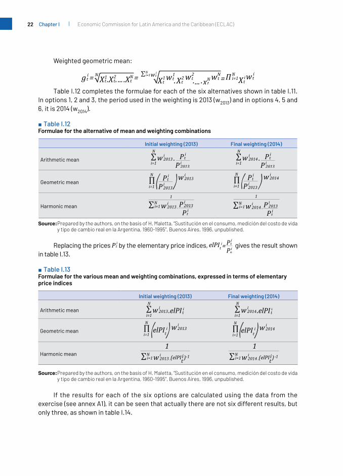
Table I.12 completes the formulae for each of the six alternatives shown in table I.11. In options 1, 2 and 3, the period used in the weighting is 2013 (w2013) and in options 4, 5 and 6, it is 2014 (w2014).
■ Table I.12 Formulae for the alternative of mean and weighting combinations
Initial weighting (2013) Final weighting (2014)
Arithmetic mean
Geometric mean
Harmonic mean
Source: Prepared by the authors, on the basis of H. Maletta, “Sustitución en el consumo, medición del costo de vida y tipo de cambio real en la Argentina, 1960-1995”, Buenos Aires, 1996, unpublished.
Replacing the prices by the elementary price indices, gives the result shown in table I.13.
■ Table I.13 Formulae for the various mean and weighting combinations, expressed in terms of elementary price indices
Initial weighting (2013) Final weighting (2014)
Arithmetic mean
Geometric mean
Harmonic mean
Source: Prepared by the authors, on the basis of H. Maletta, “Sustitución en el consumo, medición del costo de vida y tipo de cambio real en la Argentina, 1960-1995”, Buenos Aires, 1996, unpublished.
If the results for each of the six options are calculated using the data from the exercise (see annex A1), it can be seen that actually there are not six different results, but only three, as shown in table I.14.

23Index numbers and their relationship with the economy Chapter I
■ Table I.14 Rates of change in the general price level from 2013 to 2014 (equal weights)
(Percentages)
Initial weighting (2013) Final weighting (2014)
Arithmetic mean 25.0 37,5
Harmonic mean -20.0 -16.1
Geometric mean 0.0 12.2
Source: Prepared by the authors, on the basis of H. Maletta, “Sustitución en el consumo, medición del costo de vida y tipo de cambio real en la Argentina, 1960-1995”, Buenos Aires, 1996, unpublished.
One result is obtained for each mean. As the 2013 product weights are the 2014 weightings (0.5 for both wine and bread), the results for each of the means coincide, whether the weighting corresponds to 2013 or to 2014. Moreover, the result for each mean is the same as calculated above, because the weighting of each good is equal to 0.5.
In the exercise, the simple average coincides with the weighted average. However, this is generally not the case (as the weights are altered from period to period and are not constrained to be 0.5), so there are six different results. In annex A2 the quantity of the product wine is changed for 2014, and the results for the six means are recalculated, as presented in table I.15.
■ Table I.15 Rates of change in the general price level from 2013 to 2014 (variable weights)
(Percentages)
Initial weighting (2013) Final weighting (2014)
Arithmetic mean 25.0 37.5
Harmonic mean -20.0 -11.1
Geometric mean 0.0 12.2
Source: Prepared by the authors, on the basis of H. Maletta, “Sustitución en el consumo, medición del costo de vida y tipo de cambio real en la Argentina, 1960-1995”, Buenos Aires, 1996, unpublished.
It should be noted that, to determine an index number, three elements need to be defined: the elementary indices, the weights, and the formula for aggregating the elementary indices.
Under the weighted-averages approach, to check whether the formula of the weighted geometric mean is still “best”, as was the case with the simple geometric mean, the corresponding test must be performed, and its results compared with those obtained from the weighted arithmetic and harmonic means. This issue will be addressed later in sectionCwhentheaxiomaticapproachisdiscussed.Thefixed-basketapproachisnowpresented below.

24 Economic Commission for Latin America and the Caribbean (ECLAC)Chapter I
B. Fixed-basket approach
Thisapproachstemsfromthe“intuitive”ideaofdefiningabasketofproductsinagivenperiodand observing how prices vary relative to another period, while keeping the quantities constant.
ThefirstknownhistoricalrecordofthisapproachisfoundintheworkoftheBishopof Ely (United Kingdom), William Fleetwood (1656-1723), who in 1707 wrote Chronicum Preciosum. In that work, the author asked: what would £5 today buy at the prices prevailing in 1440? The £5 amount referred to a scholarship received by students at Oxford University.
To answer that question, Bishop Fleetwood had to compose a student’s “typical consumption basket”. Since there were no surveys available, he handpicked the products for the basket, including bread, drink, meat, clothes and, obviously, books. The goods handpicked by the bishop made up the basket for which the prices were to be measured.
Once the measurement was made, it was concluded that £5 in 1440 was equivalent to £28 or £30 in 1707 (Fleetwood, 1707); in other words, to maintain the purchasing power that £5 would have had in 1440, a grant of £28 to £30 should be paid in 1707, according to the value calculated from the Fleetwood basket:
Where:
:Fleetwood price index for period t
:price of good i in period t
:quantity of handpicked good i
:price of good i in period 0
If only two periods are considered in the comparison (1440 and 1707 in Fleetwood’s example), there are, in principle, two possibilities: (i) consider the initial situation (1440) as fixedtheconsumptionbasket;or(ii)considerthesituationatthefinalmoment(1707)asthefixedconsumptionbasket
As he did not have the data for the 1440 and 1707 baskets, Bishop Fleetwood chose a third alternative, which was to use a handpicked basket.
In 1823, Joseph Lowe developed the formula used by Fleetwood,11 establishing what is known as the Lowe Price Index. A comparison of the Fleetwood-Lowe formula with those developed in table I.10 shows that it is a weighted arithmetic mean:
with
11 For that reason, Diewert (1988) called Lowe the “father of price indices”.
25Index numbers and their relationship with the economy Chapter I
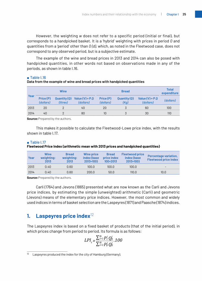
However, the weighting w does not refer to a specific period (initial or final), but corresponds to a handpicked basket. It is a ‘hybrid’ weighting with prices in period 0 and quantities from a ‘period’ other than 0 (d), which, as noted in the Fleetwood case, does not correspond to any observed period, but is a subjective estimate.
The example of the wine and bread prices in 2013 and 2014 can also be posed with handpicked quantities, in other words not based on observations made in any of the periods, as shown in table I.16.
■ Table I.16 Data from the example of wine and bread prices with handpicked quantities
YearWine Bread Total
expenditure
Price (P)(dollars)
Quantity (Q)(litres)
Value (V) = P.Q(dollars)
Price (P)(dollars)
Quantity (Q)(Kg)
Value (V) = P.Q(dollars)
(dollars)
2013 20 2 40 20 3 60 100
2014 40 2 80 10 3 30 110
Source: Prepared by the authors.
This makes it possible to calculate the Fleetwood-Lowe price index, with the results shown in table I.17.
■ Table I.17 Fleetwood Price Index (arithmetic mean with 2013 prices and handpicked quantities)
YearWine
weighting: 2013
Bread weighting:
2013
Wine price index (base 2013=100)
Bread price index
100=2013
Fleetwood price index (base 2013=100)
Percentage variation, Fleetwood price index
2013 0.40 0.60 100.0 100.0 100.0 -
2014 0.40 0.60 200.0 50.0 110.0 10.0
Source: Prepared by the authors.
Carli (1764) and Jevons (1865) presented what are now known as the Carli and Jevons price indices, by estimating the simple (unweighted) arithmetic (Carli) and geometric (Jevons) means of the elementary price indices. However, the most common and widely used indices in terms of basket selection are the Laspeyres (1871) and Paasche (1874) indices.
1. Laspeyres price index12
TheLaspeyresindexisbasedonafixedbasketofproducts(thatoftheinitialperiod), inwhich prices change from period to period. Its formula is as follows:
12 Laspeyres produced the index for the city of Hamburg (Germany).
26 Economic Commission for Latin America and the Caribbean (ECLAC)Chapter I
where:
:Laspeyres price index in period t
:price of good i in period t
:quantity of good i in period 0
:price of good i in period 0
Using the example of the basket containing just wine and bread, the result is as shown in table I.18.
■ Table I.18 Laspeyres price index and its percentage change
Year Laspeyres price index Percentage variation
2013 100 -
2014 125 25
Source: Prepared by the authors.
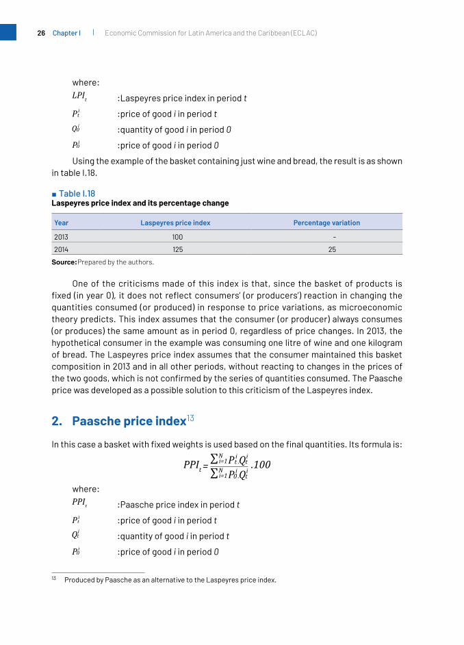
One of the criticisms made of this index is that, since the basket of products is fixed(inyear0), itdoesnotreflectconsumers’ (orproducers’)reaction inchangingthequantities consumed (or produced) in response to price variations, as microeconomic theory predicts. This index assumes that the consumer (or producer) always consumes (or produces) the same amount as in period 0, regardless of price changes. In 2013, the hypothetical consumer in the example was consuming one litre of wine and one kilogram of bread. The Laspeyres price index assumes that the consumer maintained this basket composition in 2013 and in all other periods, without reacting to changes in the prices of thetwogoods,whichisnotconfirmedbytheseriesofquantitiesconsumed.ThePaascheprice was developed as a possible solution to this criticism of the Laspeyres index.
2. Paasche price index13
Inthiscaseabasketwithfixedweightsisusedbasedonthefinalquantities.Itsformulais:
where:
:Paasche price index in period t
:price of good i in period t
:quantity of good i in period t
:price of good i in period 0
13 Produced by Paasche as an alternative to the Laspeyres price index.

27Index numbers and their relationship with the economy Chapter I
Applying this to the example gives the result shown in table I.19.
■ Table I.19 Paasche price index and its percentage change
Year Paasche price index Percentage variation
2013 100 -
2014 80 -20
Source: Prepared by the authors.
The question then is whether the Paasche index solves the Laspeyres index problem. It was noted that the Laspeyres index assumes consumer behaviour to be invariant to price changes. How is consumer behaviour treated in the Paasche index? It measures the variation in the prices of the basket of products consumed in the present projected back to the past. It assumes that the consumer has always consumed the most recent basket (the current one), regardless of past prices . What the Paasche index does is to measure the past with current consumption patterns. The consumer maintains the 2014 basket in 2013, regardlessofpricechanges.Thedataagaindonotconfirmthisassumption.Theproblemthat the Laspeyres index suffers from also appears in the Paasche index: the pattern of consumer (producer) behaviour is invariant to price changes. Consumption is the same irrespective of relative prices change. Neither index captures the substitution bias, as noted in the System of National Accounts:
“From the point of view of economic theory, the observed quantities may be assumedtobefunctionsoftheprices,asspecifiedinsomeutilityorproductionfunction. (Commission of the European Communities and others, 1993).
The following section discusses what type of mean the Laspeyres and Paasche indices are.
3. Laspeyres price index and type of mean
The formula is:
where .
This is an arithmetic mean with initial weights, corresponding to cell 1 of tables I.11, I.12 and I.13.
28 Economic Commission for Latin America and the Caribbean (ECLAC)Chapter I
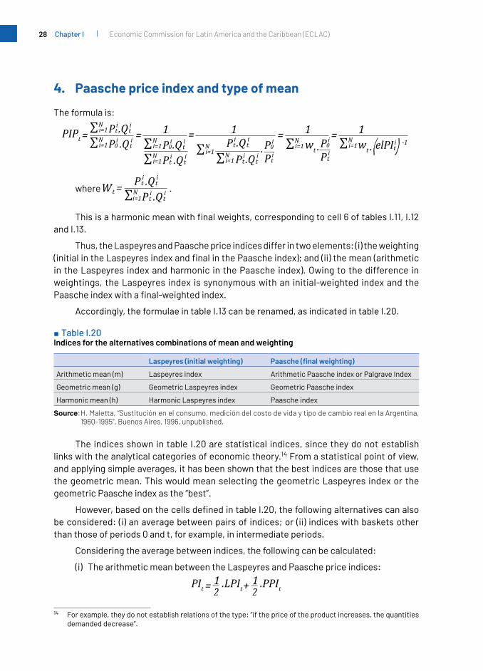
4. Paasche price index and type of mean
The formula is:
where .
Thisisaharmonicmeanwithfinalweights,correspondingtocell6oftablesI.11,I.12and I.13.
Thus, the Laspeyres and Paasche price indices differ in two elements: (i) the weighting (initialintheLaspeyresindexandfinalinthePaascheindex);and(ii)themean(arithmeticin the Laspeyres index and harmonic in the Paasche index). Owing to the difference in weightings, the Laspeyres index is synonymous with an initial-weighted index and the Paascheindexwithafinal-weightedindex.
Accordingly, the formulae in table I.13 can be renamed, as indicated in table I.20.
■ Table I.20 Indices for the alternatives combinations of mean and weighting
Laspeyres (initial weighting) Paasche (final weighting)
Arithmetic mean (m) Laspeyres index Arithmetic Paasche index or Palgrave Index
Geometric mean (g) Geometric Laspeyres index Geometric Paasche index
Harmonic mean (h) Harmonic Laspeyres index Paasche index
Source: H. Maletta, “Sustitución en el consumo, medición del costo de vida y tipo de cambio real en la Argentina, 1960-1995”, Buenos Aires, 1996, unpublished.
The indices shown in table I.20 are statistical indices, since they do not establish links with the analytical categories of economic theory.14 From a statistical point of view, and applying simple averages, it has been shown that the best indices are those that use the geometric mean. This would mean selecting the geometric Laspeyres index or the geometric Paasche index as the “best”.
However,basedonthecellsdefinedintableI.20,thefollowingalternativescanalsobe considered: (i) an average between pairs of indices; or (ii) indices with baskets other than those of periods 0 and t, for example, in intermediate periods.
Considering the average between indices, the following can be calculated:
(i) The arithmetic mean between the Laspeyres and Paasche price indices:
14 For example, they do not establish relations of the type: “if the price of the product increases, the quantities demanded decrease”.

29Index numbers and their relationship with the economy Chapter I
(ii) The harmonic mean of the Laspeyres and Paasche price indices:
(iii) Or the geometric mean of the two indices:
ThearithmeticmeanproposalwasdevelopedbyDrobisch,whospecificallyadvocatedusing this formula, thereby giving rise to the Drobisch price index.
In contrast, Fisher proposed using the geometric mean, giving rise to the Fisher price index, which, as analysed later, is considered a “superlative index”:
The result of applying the Fisher price index to the exercise reported in table I.9 is presented in table I.21.
■ Table I.21 Fisher price index (geometric mean of Laspeyres and Paasche indices)
Year Laspeyres price index (base 2013=100)
Paasche price index (base 2013=100)
Fisher price index (base 2013=100)
Percentage variation
2013 100 100 100 -
2014 125 80 100 0
Source: Prepared by the authors.
It is also possible to select cells 2 and 5 of table I.11, or the geometric Laspeyres and Paasche indices of table I.20, and obtain a geometric mean of the two, which is referred to as the Törnqvist price index:
Applying Törnqvist’s formula to the exercise in table I.9 gives the result shown in table I.22.
■ Table I.22 Törnqvist price index (geometric mean of the geometric Laspeyres and Paasche indices)
YearGeometric Laspeyres
price index (base 2013=100)
Geometric Paasche price index
(base 2013=100)
Törnqvist price index (base 2013=100)
Percentage variation
2013 100.0 100.0 100.0 -
2014 100.0 100.0 100.0 0.0
Source: Prepared by the authors.

30 Economic Commission for Latin America and the Caribbean (ECLAC)Chapter I
The Törnqvist price index can also be expressed as:
Considering the alternative of baskets other than those of periods 0 and t, a Lowe priceindexcanbedefined(accordingtothe1823formula)asfollows:
where:
As noted above, Lowe’s formula is the same as that used to calculate the Fleetwood price index, which is an arithmetic mean of the relative prices using hybrid weights w, as the prices are those of period 0 (pi
0) and the quantities refer to period b (qib).15
Young’s price index can also be calculated (according to the formula he released in 1812), as follows:
where:
Young’s formula is also an arithmetic mean of the relative prices, using a weight that corresponds to a ‘b’ period, other than periods 0 and t. It differs from the Fleetwood-Lowe price index in that the weighting is not hybrid, since the prices and quantities both refer to period b.
Young’s formula can also be expressed using a geometric mean of relative price ratios, resulting in the geometric Young price index:
P it
P io
i=1∏Nib=GYPIt=
w P1t
P1o
1b.
w P2t
P2o
2bw P N
t
P No
Nbw
. ... .
where:
Similarly, a geometric mean of quantities or weights and prices can also be calculated, to obtain the Walsh index:16
Applying this index to the example in table I.9 gives the result shown in table I.23.
15 The difference is that the Lowe index uses observed quantities whereas the Fleetwood index uses subjectively estimated ones.
16 Ascanbeseen,thefirstexpressionintheWalshpriceindexissimilartotheLowepriceindex (LoPI), as it multiplies therelativepricesbyabasket,whichturnsouttobethegeometricmeanoftheinitialandfinalbasket.

31Index numbers and their relationship with the economy Chapter I
■ Table I.23 Walsh price index
Year Wine weights
Bread weights
Wine price index(base 2013=100)
Bread price index
(base 2013=100)
Walsh price index
(base 2013=100)
Percentage variation
2013 0.50 0.50 100.0 100.0 100.0 -
2014 0.50 0.50 200.0 50.0 100.0 0.0
Source: Prepared by the authors.
The quadratic-mean-of-order-r index is also proposed, as follows:
The Fisher, Törnqvist and Walsh price indices and the quadratic-mean-of order-r index are symmetric indices, because they treat the available data symmetrically: the Fisher price index in relation to the Laspeyres and Paasche indices; the Törnqvist price index relative to the Laspeyres and Paasche geometric indices; the Walsh price index in relation to prices and quantities or weights; and the quadratic-mean-of order-r index maintains symmetry between weights and prices in both the numerator and the denominator.
Similarly, the quadratic-mean-of order-r index is a generalization of the Fisher, Törnqvist and Walsh price indices, since it is equal to the Fisher price index if r tends to 2; equal to the Walsh index if r tends to 1, and close to the Törnqvist index if r tends to 0.
Lastly, another price index formula is the Lloyd-Moulton index, which introduces an economicconceptintoitsdefinition,namelytheelasticityofsubstitution:
where σ is the value of the elasticity of substitution.17 Note that the Lloyd-Moulton index uses the same information as the Laspeyres index, while also incorporating an estimate of the elasticity of substitution. The concept of elasticity of substitution is discussed in greater detail in section E on the economic approach.
Different alternatives (and results) of price baskets or basket averages are available, andthosethatbestreflectthebehaviourofthegeneralpricelevelshouldbeselected.Noconclusion can be drawn from the pure basket analysis except that it would be better (again on logical grounds) to include more than one basket in the weights, in order to capture the substitution bias in some way. Using this criterion, the selected indices would be the quadratic-mean-of-order-r index, and the Fisher, Törnqvist and Walsh indices, but not the Laspeyres and Paasche indices.18
17 ThisconceptisdefinedinsectionE,paragraph2ofthischapter.18 Note also that, if the formulae are applied to the example proposed in table I.7, the results of the Fisher, Törnqvist
and Walsh indices are identical.

32 Economic Commission for Latin America and the Caribbean (ECLAC)Chapter I
Here again, tests, criteria or axioms have to be used, and the analysis involves using an axiomatic approach.
C. Axiomatic approach
The axiomatic approach investigates the capacity of each type of index to satisfy certain tests or properties, which enable it to be considered appropriate for measuring the behaviour of a variable, according to the following principle: “If a formula turns out to have rather undesirable properties, this casts doubts on its suitability as an index that could be used by a statistical agency as a target index” (ILO and others, 2006).
This approach proposes certain desirable properties for the indices and then attempts to determine whether the various formulae satisfy those properties. The index thatsatisfiedthepropertiescouldbeconsidered“thebest”.
Twenty basic criteria (or axioms) and two additional ones are detailed in the Consumer Price Index Manual: Theory and Practice (ILO and others, 2004) and are presented in table I.24
■ Table I.24 Basic and additional criteria applicable to the indices, according to the first axiomatic approach
Title CriterionBasic tests (20)
T1 Positivity
T2 Continuity
T3 Identity or constant prices
T4 Fixed basket or constant quantities
T5 Proportionality in current period prices
T6 Inverse proportionality in base period prices
T7 Invariance to proportional changes in current quantities
T8 Invariance to proportional changes in base quantities
T9 Commodity reversal
T10 Commensurability
T11 Time reversal
T12 Quantity reversal
T13 Price reversal
T14 Mean value test for prices
T15 Mean value test for quantities
T16 Paasche and Laspeyres bounding test
T17 Monotonicity in current prices
T18 Monotonicity in base prices
T19 Monotonicity in current quantities
T20 Monotonicity in base quantities
Additional criteria (2)
T21 Factor reversal
T22 Additivity
Source: International Labour Organization (ILO) and others, Consumer Price Index Manual: Theory and Practice, Washington, D.C., 2004 [online] https://www.ilo.org/wcmsp5/groups/public/---dgreports/---stat/documents/presentation/wcms_331153.pdf.

33Index numbers and their relationship with the economy Chapter I
Of the 20 basic tests, three are considered important in analysing the results of the index numbers: T1 (positivity), T10 (commensurability) and T11 (time reversal). Of the two additional criteria, T21 (factor reversal) can also be considered crucial.
T1 (positivity) postulates that the price index and its constituent vectors of prices and quantities should be positive:
P(P0, P1, Q0, Q1)>0T10 (commensurability) has already been analysed in the section that discusses
the tests applicable to arithmetic, harmonic and geometric means (unit change test). It postulates that the price index does not change if the units in which the products are measured are changed.
T11 (time reversal) states that the same result should be obtained whether the index change is measured forward in time (from 0 to 1), or backward (from 1 to 0):
T21 (Factor reversal) postulates that, if the price index is multiplied by the volume index, a result identical to the value index should be obtained:
Theonlyindexthatsatisfiesall20testsandalsothefactorreversaltest(T21)istheFisher price index. The only criterion that Fisher index would not satisfy is that of additivity (T22), which postulates that “changes in the subaggregates of a quantity index should add up to the changes in the totals” (ILO and others, 2004, p. 8), although the total percentage variationcanbebrokendownintoadditivecomponentsthatreflectthevariationofpricesor quantities.
The Laspeyres and Paasche indices fail three of the 20 basic tests and pass 17. The criteria on which they fail are T11 (time reversal), T12 (quantity reversal) and T13 (price reversal). Failure to satisfy T11 is considered a major defect. They also fail in T21 (factor reversal), although they satisfy it weakly; in other words, multiplying a Laspeyres price index by a Paasche volume index gives the value index; and multiplying a Paasche price index by a Laspeyres volume index also gives the value index. Both indices satisfy T22 (additivity).
Walsh’s index fails four19andsatisfies16ofthe20basictests.ItalsofailsT21(factorreversal),butsatisfiesbothT11(timereversal)andT22(additivity).
Törnqvist’s index fails nine20 and passes 11 of the 20 basic tests. It fails T21 (factor reversal)andT22(additivity),butsatisfiesT11 (timereversal).However,sinceitsatisfiesthreeofthefourcriteriaconsideredimportant—T1(positivity),T10(commensurability)andT11(timereversal)—and“approximatestheFisherindexquitecloselyusing ‘‘normal’’timeseries data that are subject to relatively smooth trends.”
19 T13 (price reversal), T16 (Paasche and Laspeyres bounding test), T19 (monotonicity in current quantities) and T20 (monotonicity in base quantities).
20 T4(fixedbasket),T12(quantityreversal),T13(pricereversal),T15(meanvaluetestforquantities),T16(Paascheand Laspeyres bounding test) and the criteria T17, T18, T19 and T20 (all referring to monotonicity).
34 Economic Commission for Latin America and the Caribbean (ECLAC)Chapter I
The axiomatic approach thus shows that the “best” index is the Fisher price index, followed by the Walsh and then the Törnqvist indices. In the proposed exercise, these three indices report 0% rates of change in the general price level. Their results coincide with the logical reasoning applied at the outset and also with the initial evaluations made using the simple geometric mean. The Fisher price index is a geometric mean of the Laspeyres and the Paasche indices. The Törnqvist price index is also a geometric mean, but of the geometric Laspeyres and Paasche indices. The Walsh price index uses geometric means to average weights and prices.
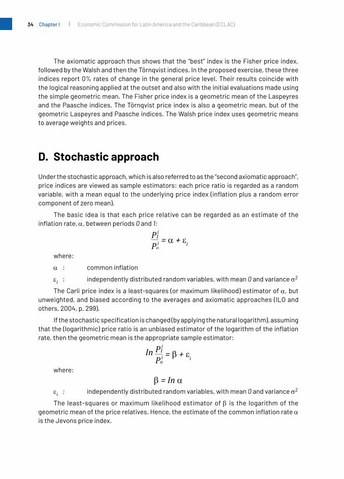
D. Stochastic approach
Under the stochastic approach, which is also referred to as the “second axiomatic approach”, price indices are viewed as sample estimators: each price ratio is regarded as a random variable,withameanequaltotheunderlyingprice index(inflationplusarandomerrorcomponent of zero mean).
The basic idea is that each price relative can be regarded as an estimate of the inflationrate,α, between periods 0 and 1:
where:
α : commoninflation
εi : independently distributed random variables, with mean 0 and variance σ2
The Carli price index is a least-squares (or maximum likelihood) estimator of α, but unweighted, and biased according to the averages and axiomatic approaches (ILO and others, 2004, p. 299).
Ifthestochasticspecificationischanged(byapplyingthenaturallogarithm),assumingthatthe(logarithmic)priceratioisanunbiasedestimatorofthelogarithmoftheinflationrate, then the geometric mean is the appropriate sample estimator:
where:
εi : independently distributed random variables, with mean 0 and variance σ2
The least-squares or maximum likelihood estimator of β is the logarithm of the geometricmeanofthepricerelatives.Hence,theestimateofthecommoninflationrateα is the Jevons price index.

35Index numbers and their relationship with the economy Chapter I
One criticism made of the Carli and the Jevons price indices, is that they assign the same weighting to all price relatives. Keynes also criticized these indices on economic grounds (ILO and others, 2004, p. 299) by arguing that, instead of “independence” between the errors in the observations, there is “connexity”: (i) a movement in the price of one commoditynecessarilyinfluencesthemovementinthepricesofothers;(ii)pricesarenotdistributed independently from each other and from quantities, but quantity movements are functionally related to price movements; and (iii) price movements must be weighted by their economic importance, that is by quantities or expenditures (the issue of weighting appears again).
Theil (1967) proposed a solution to the lack of weighting in the Jevons index, giving rise to the weighted stochastic approach:
As can be seen, the formula for this index is the same as for the Törnqvist index.
ThesamplingapproachisderivedfromTheil:thefirsttermontheleft-handsideofTheil’s formula ( ) can be interpreted as a probability pi (the expected value),21 and
the last term ( ) as the ri values22 taken by a discrete random variable, R. In other
words,theTheilpriceindexcanbedefinedintermsofprobabilities,suchthattheexpected
value of the discrete random variable R is
Generally speaking, the n discrete price relatives have a discrete statistical
probability, where the i-th probability pi is a function of the shares of output i in total expenditure in the two situations considered, and . Different price indices result, depending on how the discrete price and probability (weighting) functions are chosen (ILO and others, 2004, p. 303). Thus, each formula of the price indices analysed thus far can be expressed in terms of price functions and probabilities. In the case of the Theil price index, the discrete price function is the natural logarithm, and the probability function is the unweighted arithmetic mean.
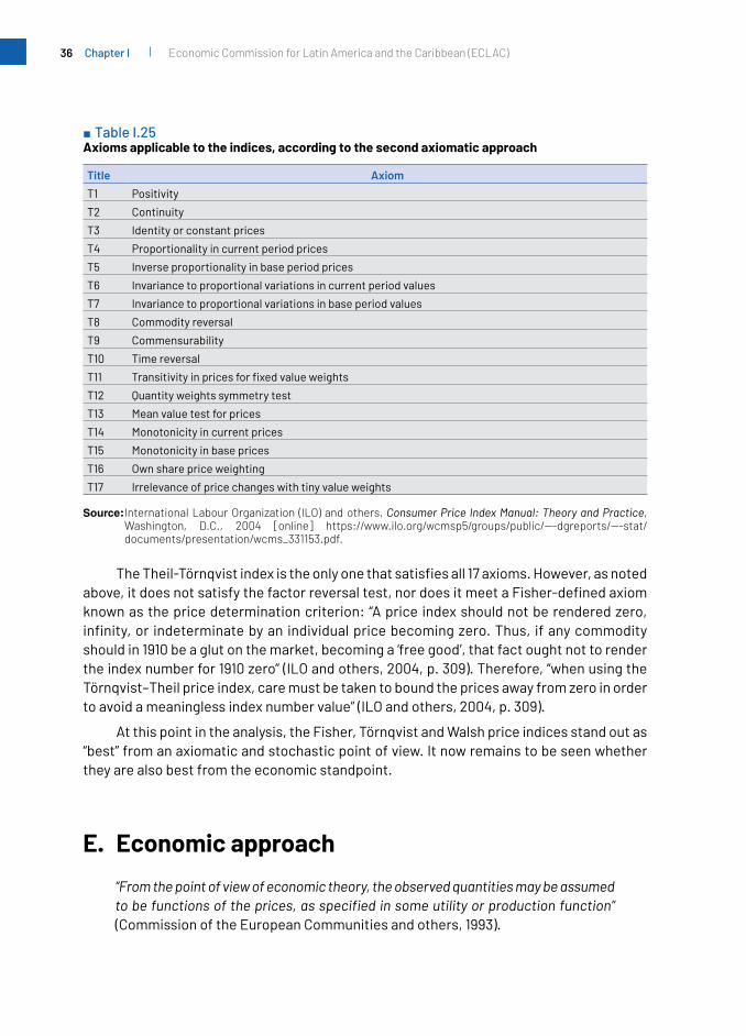
To determine which of the price index formulae is “best” from the standpoint of the sampling approach or weighted stochastic approach, axioms can again be applied to each of them, thus giving rise to the “second axiomatic approach” (ILO and others, 2004, p. 303). The applicable axioms are the 17 shown in table I.25.
21 Where p i= ½ (w0
i + wti ). Since the weights (w0
i + w1i) add up to 1 for each product i, the probabilities p
i will also sum to 1.
22 Where ri = ln (p0i / wt
i ).
36 Economic Commission for Latin America and the Caribbean (ECLAC)Chapter I
■ Table I.25 Axioms applicable to the indices, according to the second axiomatic approach
Title Axiom
T1 Positivity
T2 Continuity
T3 Identity or constant prices
T4 Proportionality in current period prices
T5 Inverse proportionality in base period prices
T6 Invariance to proportional variations in current period values
T7 Invariance to proportional variations in base period values
T8 Commodity reversal
T9 Commensurability
T10 Time reversal
T11 Transitivityinpricesforfixedvalueweights
T12 Quantity weights symmetry test
T13 Mean value test for prices
T14 Monotonicity in current prices
T15 Monotonicity in base prices
T16 Own share price weighting
T17 Irrelevance of price changes with tiny value weights
Source: International Labour Organization (ILO) and others, Consumer Price Index Manual: Theory and Practice, Washington, D.C., 2004 [online] https://www.ilo.org/wcmsp5/groups/public/---dgreports/---stat/documents/presentation/wcms_331153.pdf.
TheTheil-Törnqvistindexistheonlyonethatsatisfiesall17axioms.However,asnotedabove,itdoesnotsatisfythefactorreversaltest,nordoesitmeetaFisher-definedaxiomknown as the price determination criterion: “A price index should not be rendered zero, infinity,or indeterminatebyan individualpricebecomingzero.Thus, ifanycommodityshould in 1910 be a glut on the market, becoming a ‘free good’, that fact ought not to render the index number for 1910 zero’’ (ILO and others, 2004, p. 309). Therefore, “when using the Törnqvist–Theil price index, care must be taken to bound the prices away from zero in order to avoid a meaningless index number value” (ILO and others, 2004, p. 309).
At this point in the analysis, the Fisher, Törnqvist and Walsh price indices stand out as “best” from an axiomatic and stochastic point of view. It now remains to be seen whether they are also best from the economic standpoint.
E. Economic approach
“From the point of view of economic theory, the observed quantities may be assumed to be functions of the prices, as specified in some utility or production function” (Commission of the European Communities and others, 1993).

37Index numbers and their relationship with the economy Chapter I
Introducing the economic perspective into the analysis of index numbers means recognizing that the quantities consumed or produced are not price-independent variables; in other words, Q=f (P).23 Moreover, their dependence is guided by the postulates of economic theory, which seeks to identify the behaviour of consumers (demand theory) and producers (production theory), and then to link the two through the operation of the market.
Neoclassical economic theory postulates rational consumer and producer behaviour, assuming that: (i) the consumer tends to ‘minimize costs’ and ‘maximize utility’ by adjusting thequantitieshe/shebuysinresponsetochangesinrelativeproductprices;and(ii) theproducer also tends to ‘minimize costs’ and, at the same time, ‘maximize output’ by adjusting the quantities used as inputs or supplied as outputs in response to changes in their relative prices.
Both cases are economic optimization problems: minimize costs or maximize utilities, or both. In other words, economic theory is based on the optimizing behaviour of economic agents, whether consumers or producers, who react by varying the relative quantities they consume or produce in response to changes in relative prices.
The prices vector, P, is assumed to be a set of “observed data”; and the vector of quantities, Q, is the solution to a cost minimization and/or utility maximization problem faced by the consumer, and also the solution to a cost minimization and/or output maximization problem faced by the producer.
The economic approach is now considered from the consumer’s perspective.
1. The “real” cost of living index
Comparing the consumption basket of a consumer in 2014 with that of the same consumer in 2013 will reveal how the consumption basket has changed. The same is true if the comparison is made with the 2004 basket, when the consumer was ten years younger.
The comparison between two baskets of the same consumer between two periods involves changes in both prices and volumes;24 so the difference between the two is a difference in value. To ascertain how much of the change in value corresponds to the price variation and how much to the volume changes, the foregoing analysis is repeated.
Tocalculatethepricevariation,oneofthe“best”formulaeshouldbeused—eithertheFisher,ortheTörnqvistortheWalshindex—sincethesesatisfythepropertiesoraxiomsand therefore have statistical support, although it has not yet been determined whether they are supported in economic theory.
23 AstheArgentinescholarManuelFernándezLópez(1942-2013)recalled,thisrelationshipwasfirstpostulatedby Antoine Augustin Cournot (1801-1877), who, in 1841, published a treatise on the theory of functions and infinitesimalcalculus(Cournot,1841).Inthatwork,hearguedthatquantitiesdemandedQd are a function of prices f (P) (when prices increase, the quantities demanded decrease); and that quantities supplied Qs are also a function of prices f (P) (when prices increase, the quantities supplied increase). This revolutionized economics textswhich,untilthen,haddefinedpricesasafunctionofthequotientbetweendemandandsupply,P = f (D/S).
24 Changes in volume include both changes in the quantities of products and changes in their quality.

38 Economic Commission for Latin America and the Caribbean (ECLAC)Chapter I
The economic approach also postulates the existence of economically “best” price indices, which, from the perspective of individual consumer theory, are equal or approximate to the “true” cost of living index.
The cost of living is the minimum expenditure needed to attain a certain level of utility.
Utility is traditionally defined as the subjective feeling of pleasure that a person experiencesasaresultofconsumingaproduct.Amoreelaboratedefinition,suchasthatof Jeremy Bentham (1789), sees utility as “That property in any object, whereby it tends toproducebenefit,advantage,pleasure,good,orhappiness[…]or[…]topreventthehappening of mischief, pain, evil or unhappiness”.25
Utility is a controversial concept, because of the degree of abstraction needed to understand it and the fact that it cannot be observed. However, following Triplett (2000), it can be associated with the concept of level or standard of living.26 The standard of living is as abstract and unobservable as the level of utility, but it generates less controversy, because it is a more widely used concept and is easier to understand for economists and non-economists alike.
Assume that, in period 0, the individual consumer selects a physical basket of products, whichcanbedefinedbyapositivevectorconsistingofthen products: , and is constrained by his/her level of disposable income (or budget constraint) and the prices, P0, prevailing in period 0.
Each of those n products provide a certain level of utility or standard of living: U=f (Q). The consumer is seeking the minimum consumption expenditure C0 that would enable him/her to obtain the maximum standard of living, given his/her disposable income and preferences and the price vector P0:
The cost of living index is defined as the ratio of the minimum consumption expenditure that allows the consumer to maintain the same standard of living between two periods,givenaspecificpricevector:27
25 “Thatpropertyinanyobject,wherebyittendstoproducebenefit,advantage,pleasure,good,orhappiness[…]or[…]topreventthehappeningofmischief,pain,evilorunhappiness”.
26 Strictly speaking, the two concepts are not exactly synonymous, since one of the characteristics of utility functions is that they are monotonic transformations and establish homothetic preference relations. This implies, among other things, that the tastes and weights of the products consumed in the basket do not vary according to the consumer’s income level. However, it is well known that different tastes and spending patterns correspond to each standard of living; so existence of non-homothetic utility functions is a practical reality. Nonetheless, as explained in part 2 of this section E, the results obtained from superlative index numbers that areaccurateorclosetocost-of-livingindices,derivedfromvariousutilityfunctions,donotdiffersignificantlyaccording to whether or not preferences are assumed to be homothetic. Accordingly, the concepts of utility level and standard of living are used interchangeably in this study.
27 The origin of cost-of-living index theory is attributed to the economist Konüs (1939).

39Index numbers and their relationship with the economy Chapter I
Thus, the cost-of-living index formula involves not only the minimum expenditure of period 0, but also the minimum expenditure of another period against which the comparison is made, for example period 1.
In period 1, and given the prices in force in 1 (which are different from those prevailing in period 0), the consumption basket that would enable the consumer to maintain the same standard of living as in period 0 is C*1 where
.Accordingly:
As can be seen, the product basket is not the same as .Despite having a different product composition, however, both consumption baskets provide the same standard of living (utility). This means that when the price vector changes (between P0 and P1), the individual consumer reacts by trying to keep the standard of living obtained from consumption constant, rather than the physical quantities consumed. What remains constant is the standard of living obtained (its utility level), not the physical quantities consumed.
That is why the formula for the cost of living index is also expressed in terms of standard of living or utility U:
28
where:
: Minimum expenditure function of period 1, which depends on the utility level V0 of period 0 and price vector P1 in period 1
: Minimum expenditure function of period 0, which depends on the utility level V0 of period 0 and the price vector P0 in period 0
28 This solution for obtaining the cost of living index (also known as the Konüs-Laspeyres index) involves selecting the utility level prevailing at time 0 (U0). An alternative (which gives the Konüs-Paasche cost of living index) is to choose the utility level in period 1 (U1). Insofar as there is a negative correlation between changes in relative prices and changes in relative quantities, the Laspeyres price index is a higher bound or benchmark than the Konüs-Laspeyres ‘true’ index; and the Paasche price index is a lower bound or benchmark than the Konüs-Paasche ‘true’index.Asnotedinthefixed-basketapproach,itispossibletocalculateanaveragebetweentheLaspeyresand Paasche indices, where the geometric mean results in the Fisher price index. For the Laspeyres/Paasche indices to constitute a higher/lower benchmark, consumer (producer) preferences must be homothetic (see section E.2).

40 Economic Commission for Latin America and the Caribbean (ECLAC)Chapter I
The utility function V contained in the minimum expenditure formula is an indirect utility function.29
If maintaining the period-0 standard of living becomes more expensive between periods 0 and 1 (C*
1 > C0), the cost of living index rises; conversely, if C*1 < C0, the cost of living index falls.
However, the baskets that make up the cost-of-living index formula are not observable; they only exist in abstract in economic theory. It is therefore worth asking: what is the link between the unobservable consumption baskets, C0 and C*
1, which make up the theoretical formula of the cost of living index, and the observable baskets inferred from consumption expenditure surveys; are they the same baskets or are they different? The question can also be posed in terms of index numbers: does the cost of living index derived from unobservable economic theory coincide with any of the statistical indices obtained from observable reality?
2. Choice of a consumption basket
A consumer’s choice of the products in basket Q depends on many variables, including: his/her income level, standard of living, tastes and preferences, his/her physical and social environment, and the price vector prevailing at any given time.
All of these variables affect the choice that the individual consumer makes in real life, in a given period 0, of a basket of products at the prices prevailing in period 0, namely
. This results in a basket of prices and quantities that can actually be observed, namely .
At the starting point of the analysis, in period 0, consumption basket C0 is the same as the C0 that appears in the denominator of the formula CLI = C*
1 / C0, so it can be assumed that the consumption basket C0 is observable and can be perfectly integrated into the domain of “unobservable” economic theory.
Throughout his/her lifetime, an individual consumes successive baskets of products; for example, in period 1 the consumer will spend his/her income on the basket . But between periods 0 and 1, in addition to price changes, the consumer’s income level and/or preferences may also vary. The question then arises as to whether the observable basket C1, consisting of the quantities and the prices is the same as the unobservable basket C*1 in the numerator of the CLI 1= C*
1 /C0.
TheformuladefinedforC*1 in the cost of living index was , which differs from the consumption basket in terms of quantities ( , ), but not prices.
29 See paragraph 2 of this section E and annex A3. The indirect utility function is obtained from the direct utility function, by substituting the formula of the Xm or ordinary Marshallian quantities demanded, as obtained in the utility maximization process. While the direct utility function depends on the quantities demanded (U=f (q)), the indirect utility function V depends on the available income (budget constraint I) and the price vector P such that V=f(I, P).

41Index numbers and their relationship with the economy Chapter I
The difference between the consumption sets is that, in the unobservable basket of quantities , the only change between periods 0 and 1 is assumed to be the price vector P (which changes from P0 to P1) faced by the individual consumer; while the “observable” basket of quantities may also include variations in income level, standard of living or consumer preferences.
In other words, while the observable ratio C1/C0 is an index of value, the unobservable ratio C*
1/C0 ofthecostof livingindexisapriceindex—not justanyindex,butthe“true”price index. In both cases, prices and quantities change between periods 0 and 1; but the difference is in the standard of living provided by those quantities. In the case of the unobservable cost of living index, they provide the same standard of living in both periods (constant utility, see figure I.3), whereas the observable amounts provide a different standard of living (utility). This analysis then answers the question of whether the baskets that make up the cost of living index can match any observable basket: the answer is yes in the case of B0 but no in the case of B*
1.
The second question remains to be answered; that is, whether the ratio C*1/C0 that
definesthecostoflivingindex,andwhichincludestheunobservablecomponentC*1 in its
numerator, matches or approximates any of the index number formulae.
To answer this question, microeconomic optimization must be introduced into the analysis in terms of cost minimization or utility maximization, or both, which assumes that economic agents (consumers and producers) display optimizing behaviour.
In the theory of the individual consumer:
(i) The maximization problem involves choosing the optimal amounts for consumption, so as to maximize the standard of living given the existing price vector and income level, which operates as a budget constraint. Analytically, the problem can be expressed as:
max U (Q0, Q1) subject to I = Q0.P00+Q1.P1
0
(ii) The minimization problem is to select the optimal quantities for consumption, so as to minimize costs given the existing price vector and a certain level of utility to be achieved. This can be formulated as:
min I = Q0.P00+Q1.P1
0 , subject to U (Q0, Q1)
where:
U (Q0, Q1) :utility function (standard of living); and
I = Q0.P00+Q1.P1
0 :income or budget line, which is obtained by multiplying the amounts Q0 of product 0 and Q1 of product 1 by the prices prevailing in period 0
The solution to the problem of maximizing U(Qx, Qy) is found through “Marshallian” or “ordinary” demand quantities (Qm), whereas the minimization problem is solved through “Hicksian” or “compensated” demand (Qh). In both cases the mathematical solution is obtained using the Lagrange multiplier method.
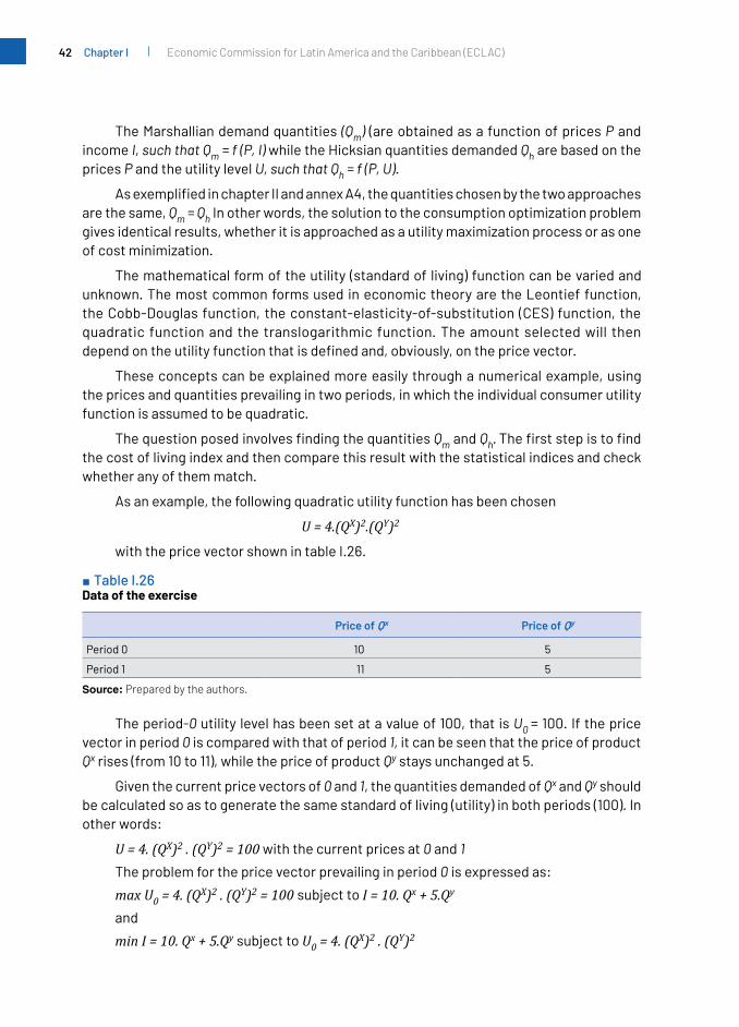
42 Economic Commission for Latin America and the Caribbean (ECLAC)Chapter I
The Marshallian demand quantities (Qm) (are obtained as a function of prices P and income I, such that Qm = f (P, I) while the Hicksian quantities demanded Qh are based on the prices P and the utility level U, such that Qh = f (P, U).
AsexemplifiedinchapterIIandannexA4,thequantitieschosenbythetwoapproachesare the same, Qm = Qh In other words, the solution to the consumption optimization problem gives identical results, whether it is approached as a utility maximization process or as one of cost minimization.
The mathematical form of the utility (standard of living) function can be varied and unknown. The most common forms used in economic theory are the Leontief function, the Cobb-Douglas function, the constant-elasticity-of-substitution (CES) function, the quadratic function and the translogarithmic function. The amount selected will then dependontheutilityfunctionthatisdefinedand,obviously,onthepricevector.
These concepts can be explained more easily through a numerical example, using the prices and quantities prevailing in two periods, in which the individual consumer utility function is assumed to be quadratic.
ThequestionposedinvolvesfindingthequantitiesQm and Qh. Thefirststepistofindthe cost of living index and then compare this result with the statistical indices and check whether any of them match.
As an example, the following quadratic utility function has been chosen
U = 4.(QX)2.(QY)2
with the price vector shown in table I.26.
■ Table I.26 Data of the exercise
Price of Qx Price of Qy
Period 0 10 5
Period 1 11 5
Source: Prepared by the authors.
The period-0 utility level has been set at a value of 100, that is U0 = 100. If the price vector in period 0 is compared with that of period 1, it can be seen that the price of product Qx rises (from 10 to 11), while the price of product Qy stays unchanged at 5.
Given the current price vectors of 0 and 1, the quantities demanded of Qx and Qy should be calculated so as to generate the same standard of living (utility) in both periods (100). In other words:
U = 4. (QX)2 . (QY)2 = 100 with the current prices at 0 and 1
The problem for the price vector prevailing in period 0 is expressed as:
max U0 = 4. (QX)2 . (QY)2 = 100 subject to I = 10. Qx + 5.Qy
and
min I = 10. Qx + 5.Qy subject to U0 = 4. (QX)2 . (QY)2

43Index numbers and their relationship with the economy Chapter I
Lagrange multipliers30 are applied to obtain the optimum demand quantities:
Qm31 = Qh
32 = (Qx = 1.58; Qy = 3.16)
Multiplying the prices by the quantities33 in period 0 gives the minimum expenditure C0 = 31.6 needed to obtain a standard of living (utility) valued at 100 (U0 = 100), which absorbs total income available at time 0 (line I0).
Graphically,theproblemissolvedinthequantitiesspace(seefigureI.1).Giventheprices prevailing in period 0 (10 for product Qx and 5 in the case of product Qy, together with the budget line or available income I0 and the indifference curves derived from the utility function U, the geometric solution of the optimization point or (observable) basket C0 chosen in period 0 is found at the point where indifference curve U0 is tangent to the budget line I0.
■ Figure I.1 Lagrange multiplier – graphical solution
Qy
3.16
Qx1.58
Optimization pointfor basket C0:
(Qx = 1.58; Qy = 3.16)
Indifference curve U0 obtained from utility function U0
Budget line I0I=10.Qx + 5.Qy
I0 U0 = 100
Source: Prepared by the authors.
InfigureI.2,theriseinthepriceofproductQx from 10 to 11 is indicated by pivoting budget line I down and to the left (from I0 to I1), while keeping its intersection with the verticalaxisatthesamepointasinfigureI.1(sincethepriceofproductQy does not change), and moving the intersection with the X-axis to the left (the price of product Qx increases). The new (observable) basket C1, selected as an optimization point, shows a consumption vector of 3.16 units of Qy and 1.44 units of Qx34.reflectingadecreaseinconsumptionoftheproduct Qx (from 1.58 to 1.44) following its price in rise.
30 The optimization process is set out in full in annex A3.31 The formula obtained from the Lagrange multipliers to calculate the Marshallian demand quantities is Xm = I /
(2 x pX) and Ym = I / (2 x pY).32 The formula obtained from Lagrange multipliers to calculate the Hicksian demand quantities is Xh = (U x pY2 /
4 x pX2)¼ and Yh = (U x pX2 / 4 x pY2)¼.33 10 x 1.58 + 5 x 3.16.34 With the same disposable income (31.6), and with the price of product Qx rising from 10 to 11, the consumption
basket is 11 x 1.44 + 5 x 3.16. Graphically, I0 pivots to I1 following the change in the price of product Qx, since changesintheslopeofthebudgetlineIreflectchangesintherelativepricesofproductsQx and Qy.

44 Economic Commission for Latin America and the Caribbean (ECLAC)Chapter I
■ Figure I.2 New situation: increase in the price of product Qx
Qy
3.16
Qx1.581.44
Basket C0:(Qx = 1.58;Qy = 3.16)
Basket C1:(Qx = 1.44;Qy = 3.16)
I0I1
U0 = 100
U1
Source: Prepared by the authors.
In the new consumption situation C1, indifference curve U1 is located below and to the left of U0, which means that the new utility level (standard of living) is lower than the value 100 obtained from U0.35
As noted above, calculating the cost of living index entails estimating the unobservable consumption set C*
1. Graphically, it involves drawing a budget line parallel to I1 (labelled I*1
andidentifiedbyadottedline),tangenttotheoriginalindifferencecurveU0, which results from the utility function U0(seefigureI.3).
■ Figure I.3 Graphical representation of the new unobservable basket
Qy
3.16
3.32
Qx1.581.44 1.51
Basket C0:(Qx = 1.58;Qy = 3.16)
Basket C*1:(Qx = 1.51;Qy = 3.32)
Basket C1:(Qx = 1.44;Qy = 3.16)
I1 I*1
U0 = 100
U1
Source: Prepared by the authors.
35 The utility level attained with the U1 indifference curve is 82.65.

45Index numbers and their relationship with the economy Chapter I
With the period-1 price vector, the optimal quantities demanded are: Qm = Qh = (Qx = 1.51;
Qy = 3.32). By multiplying the period-1 prices by those quantities demanded, the (unobservable) minimum expenditure is obtained as C*1 = 33.2 which affords the same standard of living (utility) as in period 0 equal to 100 (U0 = 100).ThisisshowninfigureI.3,where it can be seen that the observable consumption basket C0 and the unobservable consumption set C1 are located on the same U0 indifference curve, thus producing a movement “along” the U0 curve.
When faced with a rise the price of product Qx (from 10 to 11), the individual consumer reacts by decreasing his/her consumption of that product and increasing the consumption of product Qy. The exact value of the change in quantities depends on how the utility function Uisspecified,whichinthiscaseisquadratic.
■ Box I.1 Hicksian substitution and income effects
The rise in the price of product Qx reduces its consumption by 0.14 units, from 1.58 units to 1.44; this the total effect. At the same time, the consumer continues to demand the same amount of product Qy (3.16 units, total effect zero). The difference between the quantities demanded in the original basket C0 and those demanded in C*
1 represent the Hicksian “substitution effect”. Consumption set C*
1 answers the question, what basket would the consumer choose to keep utility constant at the new price ratio P1? For product Qx, the answer is 1.51 units, which is a reduction of 0.07 units (1.51 - 1.58 = -0.07). In the case of product Qy, the answer is 3.32 units, a decrease of 0.16 units (3.32 - 3.16 = 0.16). The difference between the total effect and the substitution effect is known as the “income effect”: for product Qx this is -0.07 units (-0.14 - (-0.07) = -0.07) and for product Qy it is -0.16 units (0 - 0.16 = -0.16). In the “substitution effect” the consumer moves “along” the U0 indifference curve, thus maintaining his/her utility level (standard of living). For this to be viable, the consumer must be assumed to receive an “imaginary” monetary compensation, to be able to maintain his/her monetary income and the same level of utility (standard of living) given the new price vector P1.
Source: Prepared by the authors.
Once the values of C0 and C*1 are obtained, the cost-of-living index quotient can be
calculated:
The cost of living index rises by 4.9% between period 0 and period 1. Figure I.3 shows the composition of the two consumption sets being compared in ICV1, namely C0 and C*
1.
With the price and quantity-demanded data thus obtained, the price index formulae can be applied, and the results compared with the cost-of-living index, as shown in table I.27.

46 Economic Commission for Latin America and the Caribbean (ECLAC)Chapter I
■ Table I.27 Cost of living index according to different price index formulas
Laspeyres price index
Paasche price index
Fisher price index
Laspeyres geometric
index
Paasche geometric
index
Lloyd Moulton price indexa
Törnqvist price index
Walsh price index
1.05000 1.04762 1.04881 1.04881 1.04881 1.04881 1.04881 1.04881
Source: Prepared by the authors.a σ tends to 1.
As can be seen, the formulae of the Fisher, Lloyd-Moulton, Törnqvist and Walsh price indices, as well as those of the geometric Laspeyres and Paasche indices, all give a 4.9% increase in the cost of living index.
Ofalltheseformulae,theexactindexistheFisherpriceindex(highlightedintable I.27),since “if the preferences can be represented by a homogeneous quadratic utility function, theFisherindexprovidesanexactmeasureofthe[costoflivingindex]”(ILOandothers,2004). For this reason, the Fisher price index is an “exact” index, because it gives an exact result; in other words, it tracks the exact evolution of the cost of living index that results from the quadratic utility function.
Similarly, other “exact” indices can be defined for cost-of-living indices that are derived from other utility functions, as detailed in table I.28.
■ Table I.28 Exact price indices for different cost-of-living indices derived from utility functions
Price index Utility function from which the cost of living index is derived
Fisher price index Quadratic
Törnqvist price index Translogarithmic
Geometric Laspeyres index (GLI) Cobb-Douglas
Lloyd-Moulton price index Constant elasticity of substitution
Laspeyres price index/Paasche price Index Leontief
Source: Prepared by the authors.
Examples are given below for each of these functions (see table I.29).36 In each case, the cost of living index and the exact price index are highlighted.
■ Table I.29 Results of the main price indices for selected utility functions
A. Cobb-Douglas utility function
Utility function Parameters Quantities ( , )Cobb-Douglas ( , ) = =
. ( ) . ( )10
0.6 8.91 11.88 100 148.6
0.4 8.58 12.58 100 157.3 1.05885
36 SeeDelfino(2002)forasimilaranalysis.

47Index numbers and their relationship with the economy Chapter I
Laspeyres price index (LPI)
Paasche price index
(PPI)
Fisher price index(FPI)
Geometric Laspeyres
index(GLI)
Geometric Paasche
index(GPI)
Lloyd Moulton
price index (LMPI) a
Törnqvist price index
(TPI)
Walsh price index(WPI)
1.06000 1.05769 1.05885 1.05885 1.05885 1.05885 1.05885 1.05885a σ tends to 1.
B. Constant-elasticity-of-substitution (CES) utility function
Utility function Parameters Quantities( , )
CES
. ( ) ]
( , ) = = . [ . (
1
0.3
0.7 41.32 153.04 100 1 178.4
-0.17647 39.21 157.47 100 1 218.6 1.03414
1
LPI PPI FPI GLI GPI LMPIa TPI WPI
1.03506 1.03324 1.03415 1.03398 1.03414 1.03414 1.03414 1.03415a σ = 0.85.
C. Translogarithmic utility function
Utility function Parameters Quantities
( , )TRANSLOG
( , )) )= ( )
+ ( )
+ ( )
+ . ( ) . ( )
)2+ . ( ) . ( )+ . ( )2 + . (
1
0.5
0.5 73.34 137.72 100 1.422
0.0125 70.33 144.02 100 1.493.8 1.05049
0.0125
-0.0125
-0.0125
LPI PPI FPI GLI GPI LMPIa TPI WPI
1.05157 1.04941 1.05049 1.05038 1.0560 1.05049 1.05049 1.05049a σ = 0.91.
D. Leontief utility function
Utility function Parameters Quantities ( , )Leontief
( , ) = =( ; ) 0.4 40 60 100 700
0.6 40 60 100 740 1.05714
LPI PPI FPI GLI GPI LMPIa TPI WPI
1.05714 1.05714 1.05714 1.05597 1.05831 1.05597 1.05714 1.05714
Source: Prepared by the authors.a σ tends to 1.
Table I.29 (conclusion)

48 Economic Commission for Latin America and the Caribbean (ECLAC)Chapter I
As can be seen, the result depends on the utility function that supposedly rationalizes the consumer’s behaviour; there will be as many solutions for the cost of living index as there are utility functions. One could then make the following proposal: “Show me your utility function and I’ll tell the price index that corresponds exactly to the cost of living index”.
As noted above, economic theory rules out utility functions that postulate that the individual consumer does not change the quantities demanded in response to price changes, or that he/she always reacts in the same way to such changes, regardless of the level of consumption or scale. In economic theory, the degree to which an individual consumer reacts to price changes is measured by the concept of elasticity of substitution:
“the elasticity of substitution, denoted as σ, is a measure of the change in the quantity of, say, item i relative to item j, that would arise from a unit change in the price of item i relative to item j. A value of zero would imply that a change in price would lead to no substitution between the consumption of items and σ>1 implies that the change in expenditure arising as a result of substituting items is positive: it is worth switching (ILO and others, 2004, Appendix 8.2, paragraph 1).
An extreme case is the “Leontief-type” consumer, who does not react to price changes (his/her elasticity of substitution is equal to 0), and thus keeps the consumption basket exactly the same. That is why Leontief’s utility function is ruled out as representative of consumer behaviour.37
It is also recognized that “consumers’ preferences are unlikely to conform exactly” to the quadratic functional form (ILO and others, 2004, p. 11).
Moreover, although still used, the Cobb-Douglas and CES functional forms have lost popularity, among other reasons, because they impose a priorifixedvaluesfortheelasticitiesof substitution (1 in the case of the Cobb-Douglas and constant in the CES function).38
The translogarithmic function39 and other functional forms, such as generalized Cobb-Douglas or generalized Box-Cox, have gained traction, since they do not impose restrictions on the values of the elasticity of substitution and are more realistic.
Diewert (1976) showed that the Fisher, Törnqvist and Walsh price indices are superlative indices, when these statistical indices are accurate for a cost of living index based on “a certain
37 Although, the consumer might rationalize his/her behaviour along “Leontief” lines for certain groups of products, by demanding the same amount irrespective of price changes. This type of behaviour can be applied to goods thatareconsidered“inelastic”orinflexiblewithrespecttochangesintheirprices,suchasmedicines,fuelsand “vices” (drugs or alcoholic beverages). In such cases, large price variations do not elicit changes in the quantities demanded, for reasons of necessity in consumption.
38 According to laboratory simulations using basic prices in the United States spanning December 1986 to December 2000, elasticities of substitution are unstable over time within the range of 0.06 to 2.78. See Cage, Greenlees and Jackman (2013), Introducing the Chained Consumer Price Index, Paris, France. On the other hand, Maletta (1996)notesthat“[m]ostempiricalstudiesindifferentcountriesandperiods,usingdifferentassumptionsabout consumer behaviour, have found elasticities of substitution with values concentrated between 0.3 and 1.5. Only certain goods with very rigid demand (such as salt) have elasticities of substitution close to zero; and only highly substitutable goods have elasticities of substitution greater than 2”.
39 Christensen, Jorgenson and Lau (1975) introduced this function in the economic literature.

49Index numbers and their relationship with the economy Chapter I
functionalformandwhenthatfunctionalformisflexible”40 (ILO and others, 2004, p. 11). Flexible functions are those that can provide a second-order approximation to other functions that are twice-differentiable around the same point or within a certain range of values.41
Thus, quadratic and translogarithmic functions can give a “second order differential approximationtoavastrangeofneoclassical-typeutilityfunctions”(Maletta,1996,p. 39).These indices are considered very close approximations of the true consumer cost of living index, even relaxing the assumption that they maximize their utility in ways that are compatible with demand theory, and even though the demand function has not been specifiedorestimated(Maletta,1996,p.39).
Since the utility function is unobservable, its mathematical form is generally unknown; so if one calculates any of the superlative indices (the Fisher, Törnqvist or Walsh indices), one canbesurethattheyconstitutea“fairlycloseapproximationtotheunderlying[costoflivingindex] in a wide range of circumstances” (ILO and others p.11) and therefore approximate the results of an underlying cost of living index with an unknown utility function.
The practical results of applying the Fisher and Törnqvist superlative indices show that all bilateral comparisons (between two periods, e.g. 0 and 1) “differ by just 0.1% on average”, so their results are likely to be “very similar” and for ‘normal’ time-series data, these three indices will give virtually the same answer” (ILO and others, 2004, p. 325).
This idea can be summarized as follows: the precise specification of the utility function is unimportant, because the calculation of a superlative index is certain to produce a result that approximates to the underlying cost of living index, which can be derived from a wide range of utility functions. As Maletta (1996, p. 61) argues, if all the ideal indices give very similar results, and each of them is accurate or superlative for several frequently used utility functions, then specifying and estimating the utility function is no longer a requirement for estimating the cost of living index.
The Fisher, Törnqvist and Walsh superlative indices are “best” because they are supported economically, axiomatically and stochastically. In general, these superlative indicesarewithintherangedefinedbytheLaspeyresandPaascheindices.Indeed,fromthe consumer’s perspective, the Laspeyres price index represents an upper bound for the cost of living index, and the Paasche price index represents a lower bound.42
From the standpoint of producer theory, the reverse is the case, with the Paasche priceindexconstitutingaceilingandtheLaspeyresprice indexafloor.43 These biases arise because the indices in question do not incorporate the substitution effect.
40 This term is introduced by Diewert (1974, p. 133).41 Given an arbitrary function f*, the class of homogeneous functions contains a homogeneous quadratic function
, which is a second-order approximation to f* in a q* environment. So, fisflexible,suchthatthelevelandallfirst-andsecond-orderpartialderivativescoincideinq*.
42 For this to happen, quantities and prices need to move in opposite directions, for example if prices rise, quantities need to fall.
43 For this to happen, quantities and prices need to move in the same direction, for example if prices rise, quantities must also rise.
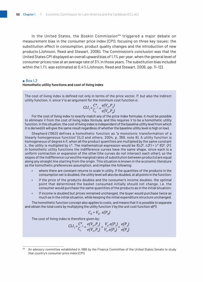
50 Economic Commission for Latin America and the Caribbean (ECLAC)Chapter I
In the United States, the Boskin Commission44 triggered a major debate on measurement bias in the consumer price index (CPI), focusing on three key issues: the substitution effect in consumption, product quality changes and the introduction of new products (Johnson, Reed and Stewart, 2006). The Commission’s conclusion was that the United States CPI displayed an overall upward bias of 1.1% per year, when the general level of consumer prices rose at an average rate of 3% in those years. The substitution bias included within the 1.1% was estimated at 0.4% (Johnson, Reed and Stewart, 2006, pp. 11–12).
■ Box I.2 Homothetic utility functions and cost of living index
44 An advisory committee established in 1995 by the Finance Committee of the United States Senate to study that country’s consumer price index (CPI).
Thecostoflivingindexisdefinednotonlyintermsofthepricevector,P, but also the indirect utility function, V, since V is an argument for the minimum cost function e:
For the cost of living index to exactly match any of the price index formulae, it must be possible to eliminate V from the cost of living index formula, and this requires V to be a homothetic utility function. In this situation, the cost of living index is independent of the baseline utility level from which it is derived (it will give the same result regardless of whether the baseline utility level is high or low).
Shephard (1953) defines a homothetic function as “a monotonic transformation of a linearly homogeneous function” (ILO and others, 2004, p. 369, note 8). A utility function is homogeneous of degree k if, when all the product quantities are multiplied by the same constant λ, the utility is multiplied by λk. The mathematical expression would be f(λQx, λQy) = λk f(Qx, Qy). In homothetic utility functions the indifference curves have the same shape, since each is a uniform contraction or expansion of the other (the curves do not intersect each other), so the slopes of the indifference curves (the marginal rates of substitution between products) are equal along any straight line starting from the origin. This situation is known in the economic literature as the homothetic preferences assumption, and implies the following:
• where there are constant returns to scale in utility, if the quantities of the products in the consumption set is doubled, the utility level will also be doubled, at all points in the function;
• if the price of the products doubles and the consumer’s income doubles, the optimal point that determined the basket consumed initially should not change, i.e. the consumer would purchase the same quantities of the products as in the initial situation;
• if income is doubled but prices remained unchanged, the buyer would purchase twice as much as in the initial situation, while keeping the initial expenditure structure unchanged.
The homothetic function concept also applies to costs, and means that it is possible to separate and obtain the total costs by multiplying the utility function V by the unit cost function e(P):
The cost of living index is therefore given by:

51Index numbers and their relationship with the economy Chapter I
The cost of living index is no longer a ratio of expenditures but a ratio of prices, and the utility function has disappeared from the argument, so a cost of living index can be expressed in cardinal terms. This also means, for example, that if the prices of the products in the basket double, the cost of living index (constant cost returns to scale) doubles, regardless of the utility level.
Although this homothetic preferences assumption “is not strictly justified from the viewpoint of actual economic behaviour” (ILO and others, 2004, paragraph 17.18), as it implies “equal expenditure structures for all income levels” (Maletta, 1996, p. 10), “it can be seen that the assumption of homotheticity will usually not be empirically misleading in the index number context” (ILO and others, 2004, p. 316, note 9).
If preferences are assumed non-homothetic, then returns to scale vary, such that some points in the function may display constant returns to scale, while others may display increasing or decreasing returns; and, more realistically, cost structures vary according to different income levels.Inthiscase,theuseoftheTörnqvist-Theilindexisjustified(ILOandothers,2004).Sincethisindex is superlative and, as noted above, it yields very similar results to those of the other superlative indices(FisherandWalsh),thecostoflivingindexwillnotdiffersignificantly,regardlessofwhetherpreferences are assumed homothetic or non-homothetic. In fact, as Maletta (1996) notes, indirect translogarithmic utility functions do not have to be homothetic (Christensen, Jorgenson and Lau, 1975, p. 368). Furthermore, Diewert (1976, pp. 122-123) shows that the Törnqvist-Theil index is accurate for the non-homothetic translogarithmic functional form.
In conclusion, the superlative formulae of the Fisher, Törnqvist and Walsh indices give similar results for the cost of living index, irrespective of the mathematical form of the utility function, or whether homothetic preferences are assumed or not, and regardless of whether consumers have altered their consumption basket.
Source: Prepared by the authors, on the basis of International Labour Organization (ILO) and others, Consumer Price Index Manual: Theory and Practice, Washington, D.C., 2004 [online] https://www.ilo.org/wcmsp5/groups/public/---dgreports/---stat/documents/presentation/wcms_331153.pdf; H. Maletta, “Sustitución en el consumo, medición del costo de vida y tipo de cambio real en la Argentina, 1960-1995”, Buenos Aires, 1996, unpublished; L. Christensen, D. Jorgenson and L. Lau, “Transcendental logarithmic utility functions”, The American Economic Review, vol. 65, No. 3, American Economic Association, 1975 [online] http://www.jstor.org/stable/1804840; and W. E. Diewert, “Exact and superlative index numbers”, Journal of Econometrics, No. 4, Amsterdam, North-Holland Publishing Company, 1976 [online] http://www.researchgate.net/publication/4856926_Exact_and_superlative_index_numbers.
■ Figure I.4 Functions with homothetic preferences
Qy
Qx
U1
U0
U2
Source: Prepared by the authors.
■ Box I.2 (concluded)

52 Economic Commission for Latin America and the Caribbean (ECLAC)Chapter I
■ Figure I.5 Functions with non-homothetic preferences
Qy
Qx
U1
U0
U2
Source: Prepared by the authors.

Chapter IIDirect comparison and the producer perspective
The approaches made from the consumer’s point of view can also be applied from the standpoint of the producer, so the axiomatic, stochastic and economic approaches will again beanalysedinthischapter.However,theeconomicapproachneedsanumberofclarifications.
The cost-of-living index theory discussed in the previous chapter assumes that consumers behave optimally and are price takers.1 Similarly, price index theory from the producer’s standpoint2 presupposes the existence of a perfect competitive market structure, and also assumes that producers behave optimally and are price takers.
If market structures other than perfect competition prevail (such as monopolistic competition, monopoly or oligopoly), then the producer’s actions may affect market prices. In this case, the economic approach, as presented, is not valid and must be amended to take account of such situations.
As noted above, introducing the economic perspective into index-number analysis means recognizing that quantities consumed or produced are not price-independent variables. The optimistic and rational behaviour attributed to the producer leads it to “minimize costs” and, at the same time, to “maximize production” by adjusting the quantities it uses as inputs or those it supplies as outputs in response to changes in their relative prices.
From the producer perspective, the following need to be estimated: (i) the production function, which represents the industrial-technological relationship between output and the factor inputs, and, within that framework, returns to scale and the level of output; (ii) the cost function, which makes it possible to determine the minimum cost of producing a given basket of products; (iii) returns to scale and costs; and (iv) the elasticity of substitution between the factors of production (inputs).
1 This theory was developed by Konüs (1939).2 Prepared by Fisher and Shell (1972), and by Archibald (1977).

54 Economic Commission for Latin America and the Caribbean (ECLAC)Chapter II
Theseconceptscanalsobedefinedinconsumertheory(infact,someofthemwerediscussed in chapter I). The following analogies can be established: the concept of utility U is replaced by production Q; the utility function U(Qx, Qy) is reinterpreted as the production function Q(QK, QL); the products that make up the consumption basket, Qx and Qy, are replaced by the factor inputs, QK and QL (capital and labour, respectively); and the product prices, Px and Py, are replaced by factor prices, PL and PK. Lastly, it is important to note that while the level of utility U cannot be observed, the level of production Q is observable.
The functional forms that the production function can adopt are analogous to those of the consumer utility function described in the previous chapter. Accordingly, the Leontief, quadratic, constant elasticity of substitution (CES), Cobb-Douglas or translogarithmic formulae are all possible.
The production function f(K, L) will be analysed through a microeconomic lens, assuming constant elasticity of factor substitution:3
f (K, L) = Q = A * (α * K-ρ + β L-ρ )-ν/ρ
where:
K: capital input
L: labour input
Q: output
A: technology parameter
α: parameter representing the ratio of capital K to total income
β: parameter representing the ratio of labour L to total income (α + β = 1)
ρ: parameter representing the Allen partial elasticity of substitution σKL, where ρ = (σ-1)/σ
ν: parameter representing the return to scale or degree of homotheticity of the function, such that ν = 1 implies constant returns to scale (a homogeneous function of degree 1); ν < 1 means decreasing returns to scale (a homogeneous function of degree n < 1), and ν > 1 indicates increasing returns to scale (a homogeneous function of degree n > 1)
Assume the following parameter values for the CES function: A = 1, α= 0.3, β = 0.7(note that α + β = 1 isverified), ρ = 0.17647 (so σKL= 0.85) and ν = 1.
Accordingly, it is a function of constant returns to scale and homogeneous of degree 1:
Q = 1 * (0.3 K -0.17647 + 0.7 L -0.17647) - ( 1 / 0.17647)
Solving for L gives:
L = (Q ^ -0.17647 / 1 - 0.3 * K -0.17647) / 0.7) 1 / 0.017647
3 This production function is also referred to as direct, and depends on the factors of production: Q = f (K, L). It differs from the indirect production function which depends on the factor prices and the budget available to remunerate them for their participation in the production process Q = G (R, PK, PL).

55Index numbers and their relationship with the economy Chapter II
Thus, for example, starting from an initial situation with a production level of 100 units (Q=100) and a capital input of 100 units (K=100), it is possible to use the CES production function to determine the number of units labour (L) needed (see table II.1). The result is 100.
■ Table II.1 Initial situation
Q α β K L
100 0.3 0.7 100 100
Source: Prepared by the authors.
If the capital input is increased by one unit successively, the relative decrease in labour input can be calculated (see table II.2).4
■ Table II.2 Successive unit increases in the factor K
Q α β K L
100 0.3 0.7 100 100.00
100 0.3 0.7 101 99.57
100 0.3 0.7 102 99.16
100 0.3 0.7 103 98.75
100 0.3 0.7 104 98.34
100 0.3 0.7 105 97.94
100 0.3 0.7 106 97.55
100 0.3 0.7 107 97.17
100 0.3 0.7 108 96.79
100 0.3 0.7 109 96.41
100 0.3 0.7 110 96.04
100 0.3 0.7 111 95.68
100 0.3 0.7 112 95.32
100 0.3 0.7 113 94.97
100 0.3 0.7 114 94.63
100 0.3 0.7 115 94.28
100 0.3 0.7 116 93.95
100 0.3 0.7 117 93.62
100 0.3 0.7 118 93.29
100 0.3 0.7 119 92.96
100 0.3 0.7 120 92.65
100 0.3 0.7 121 92.33
Source: Prepared by the authors.
4 Production becomes more capital-intensive and less labour-intensive.

56 Economic Commission for Latin America and the Caribbean (ECLAC)Chapter II
Doubling the quantities of capital and labour used for each K-L combination, as shown in table II.2, means that output Qalsodoubles(reflectingconstantreturnstoscale) (seetable II.3).
■ Table II.3 Doubling of factors K and L
K L Q
200 200.00 200
202 199.15 200
204 198.31 200
206 197.49 200
208 196.68 200
210 195.89 200
212 195.10 200
214 194.33 200
216 193.57 200
218 192.82 200
220 192.09 200
222 191.36 200
224 190.65 200
226 189.95 200
228 189.25 200
230 188.57 200
232 187.89 200
234 187.23 200
236 186.58 200
238 185.93 200
240 185.29 200
242 184.67 200
Source: Prepared by the authors.
However, in this exercise, an important element has been omitted, namely factor prices, which determine the budget constraint R = f(P,F). Given the price vector P, factor demand F will be determined by the available budget.
Assuming factor prices of PK = 10 (one unit of the factor service provide by capital is pricedatUS$ 10)and PL = 5 (the unit price of labour services is US$5), the budget constraint will be given by the following equation:
R = PK . K + PL . L = 10 . K + 5 . L
The (direct) production function Q = f (K, L) can be used to determine different combinations of the factors K and L needed to produce different quantities of output Q,

57Index numbers and their relationship with the economy Chapter II
depending on the available technology. However, it does not establish a relation with factor prices, so it does not indicate how many units of K and L should be used to obtain the maximum output Q, given their current prices, PK and PL, and the budget constraint R. This maximumoutputlevelmustbeefficient,inotherwordscompatiblewithaminimumlevelof costs (minimum factor demand given their prices).
Analogously to the discussion in consumer theory, two problems emerge from this analysis: one related to the maximization of production and the other to the minimization of costs. The maximization analysis is also known as the primal problem, and the minimization analysis is known as the dual.
The primal problem entails selecting optimal levels of demand for factors K and L, so as to obtain a maximum level of output Q, given the existing price vector, (PK, PL), and a budget constraint R. Analytically, it can be expressed as follows:
max Q(K, L), subject to R = K.PK0 + L.PL0
In contrast, the dual involves selecting the optimal levels of demand for factors K and L,suchthatcostsareminimized,giventheexistingfactorpricevectorandthespecificproduction level to be achieved. It can be formulated as:
max Q(K, L), subject to R = K.PK0 + L.PL0
where:
Q(K, L) is production function Q, and
R = K.PK0 + L.PL0 is the budget line that results from multiplying the quantities of the inputs, K and L, by their prices in period 0, namely PK0 and PL0.
The problem of maximizing Q (K, L)issolvedbyfindingthe“Marshallian”or“ordinary”factor demand quantities (Km and Lm). The solution to the minimization problem involves calculating the “Hicksian” or “compensated” quantities (Kh and Lh). In both cases, the mathematical solution is obtained using Lagrange multipliers.
The Marshallian demand quantities (Km and Lm) are obtained on the basis of prices (PK and PL) and the budget constraint R, such that, Km = f (Pk, R) and Lm = f (PL, R). The Hicksian quantities demanded (Kh and Lh) are a function of prices (PK and PL) and the production level Q, Kh = f (PK, Q) and Lh = f (PL, Q).
Analogously to the consumer theory result , in producer theory the quantities selected by the two methods coincide, Km = Kh and Lm = Lh. In other words, the solution to the output optimization problem is identical, whether obtained through output maximization or through cost minimization.
As noted above, the mathematical form of the production function can be varied and unknown. The functional forms most widely used in economic theory are the Leontief, Cobb-Douglas, CES function, quadratic function and translogarithmic functions.

58 Economic Commission for Latin America and the Caribbean (ECLAC)Chapter II
Thequantityselectedwillthendependontheproductionfunctiontobedefined,andobviously on the prevailing price vector and the budget constraint.
The CES production function selected was:
Q = 1 * (0.3 K -0.17647 + 0.7 L -0.17647) - ( 1 / 0.17647)
The exercise consists of obtaining the quantities (Km and Kh; Lm and Lh) that will make it possible to attain maximum output Q, given the period 0 price vector (PK0 = 10 and PL0 = 5) andanavailablebudgetofUS$ 1,178.4topaythefactorcost.
The maximization problem can be expressed mathematically as:
max subject to
and the cost minimization problem is given by:
min subject to
Applying Lagrange multipliers,5 the optimum quantities demanded are: Km = Kh and Lm = Lh (K = 41.32, L= 153.04).6
Multiplying the current prices by the quantities obtained7 in period 0 gives a budget constraintofUS$ 1,178.4,whichallowsforaproductionlevelof100(Q0 = 100).
Accordingly, the solution to the initial maximization problem is that, if the current factor prices are PK0 = 10 and PL0=5,thebudgetisUS$ 1,178.4anditisdesiredtoproduce100 unitsofQ, then the optimal factor combination (Marshallian demand) is 41.32 units of K and 153.04 units of L to be used in the production process (given the CES function described).
The solution to the minimization problem is as follows: if the aim is to produce 100 units of Q, current factor prices are PK0 = 10 and PL0 = 5 and it is desired to minimize costs, then the optimum factor combination (Hicksian demand) to be used in the production process is 41.32 units of K and 153.04 units of L (given the CES function as described). The factor demand basket, given the prices prevailing in period 0, isdefinedasfollows:C0 = (K=41.32 ; L=153.04).
The solutions to the output maximization and cost minimization problems are identical intermsoftheamountofeachfactordemanded.Inthefirstcase,theaimistoobtainthedemand for factors of production for maximum output, given their prices and the budget constraint R. In the second case, the aim is also to calculate factor demand, this time minimizing the cost, given the quantities Q to be produced and the prevailing factor prices.
While solving the problem of maximizing Q (K, L) and obtaining the Marshallian factor demands,anequationwillalsobeobtainedthatdefinestheindirectproductionfunction
5 The complete optimization process is set out in annex A4.6 The formula obtained by using Lagrange multipliers to calculate the Marshallian quantities demanded is:
Km=( α . PL ) σ . R / ( ασ . PK . PL σ + βσ . PL . PKσ) and Lm = ( β . PK ) σ . R / ( βσ . PL . PK σ + ασ . PK *PL
σ).7 10 x 41.32 + 5 x 153.04.
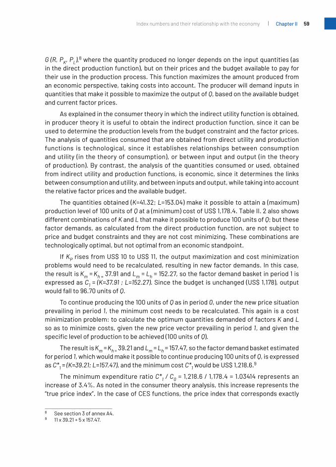
59Index numbers and their relationship with the economy Chapter II
G (R, PK, PL),8 where the quantity produced no longer depends on the input quantities (as in the direct production function), but on their prices and the budget available to pay for their use in the production process. This function maximizes the amount produced from an economic perspective, taking costs into account. The producer will demand inputs in quantities that make it possible to maximize the output of Q, based on the available budget and current factor prices.
As explained in the consumer theory in which the indirect utility function is obtained, in producer theory it is useful to obtain the indirect production function, since it can be used to determine the production levels from the budget constraint and the factor prices. The analysis of quantities consumed that are obtained from direct utility and production functions is technological, since it establishes relationships between consumption and utility (in the theory of consumption), or between input and output (in the theory of production). By contrast, the analysis of the quantities consumed or used, obtained from indirect utility and production functions, is economic, since it determines the links between consumption and utility, and between inputs and output, while taking into account the relative factor prices and the available budget.
The quantities obtained (K=41.32; L=153.04) make it possible to attain a (maximum) production level of 100 units of Qata(minimum)costofUS$ 1,178.4.TableII.2alsoshowsdifferent combinations of K and L that make it possible to produce 100 units of Q; but these factor demands, as calculated from the direct production function, are not subject to price and budget constraints and they are not cost minimizing. These combinations are technologically optimal, but not optimal from an economic standpoint.
If KP risesfromUS$ 10toUS$ 11, theoutputmaximizationandcostminimizationproblems would need to be recalculated, resulting in new factor demands. In this case, the result is Km = Kh = 37.91 and Lm = Lh = 152.27, so the factor demand basket in period 1 is expressed as C1 = (K=37.91 ; L=152.27).Sincethebudgetisunchanged(US$ 1,178),outputwould fall to 96.70 units of Q.
To continue producing the 100 units of Q as in period 0, under the new price situation prevailing in period 1, the minimum cost needs to be recalculated. This again is a cost minimization problem: to calculate the optimum quantities demanded of factors K and L so as to minimize costs, given the new price vector prevailing in period 1, and given the specificlevelofproductiontobeachieved(100unitsofQ).
The result is Km = Kh = 39.21 and Lm = Lh = 157.47, so the factor demand basket estimated for period 1, which would make it possible to continue producing 100 units of Q, is expressed as C*1 = (K=39.21; L=157.47), and the minimum cost C*1wouldbeUS$ 1,218.6.
9
The minimum expenditure ratio C*1 / C0 = 1,218.6 / 1,178.4 = 1.03414 represents an increase of 3.4%. As noted in the consumer theory analysis, this increase represents the “true price index”. In the case of CES functions, the price index that corresponds exactly
8 See section 3 of annex A4.9 11 x 39.21 + 5 x 157.47.

60 Economic Commission for Latin America and the Caribbean (ECLAC)Chapter II
to the index derived from the minimum cost ratio is that proposed by Lloyd-Moulton, as definedinthepreviouschapter:
where σ is the Allen partial elasticity of substitution σKL, which is obtained from the parameter ρ through the ratio ρ = (σ-1) / σ.
The data for the parameters of the CES production function given at the start of the exercise included the following: σKL= 0.85 (ρ = 0.17647).
Calculating the Lloyd-Moulton price index based on the price vectors prevailing in periods 0 and 1, produces a value of 1.03414, which exactly matches the “true” price index derived from the CES production function. The complete analysis of the CES production function is given in Annex A4.

Chapter IIIIndirect comparison and chain-linked indices
A. Indirect comparison
Supposethatastatisticalofficehaspriceandquantitydata(seetablesIII.1andIII.2)fortheperiod 2013-2017 and selects a Fisher price index to calculate the general price level (see table III.3).
■ Table III.1 Prices used in the indirect comparison exercise, 2013-2017
Periods Agriculture Energy Manufacturing industry
Information technology Services Communications
2013 1.0 1.0 1.0 1.0 1.0 1.0
2014 1.3 2.0 1.3 0.7 1.4 0.8
2015 1.0 1.0 1.5 0.5 1.7 0.6
2016 0.7 0.5 1.6 0.3 1.9 0.4
2017 1.0 1.0 1.7 0.2 2.0 0.2
Source: Prepared by the authors.
■ Table III.2 Quantities used in the indirect comparison exercise, 2013-2017
Periods Agriculture Energy Manufacturing industry
Information technology Services Communications
2013 30 10 40 10 45 5
2014 28 8 39 13 47 6
2015 30 11 38 30 50 8
2016 32 14 39 60 56 13
2017 29 12 40 100 65 25
Source: Prepared by the authors.

62 Economic Commission for Latin America and the Caribbean (ECLAC)Chapter III
■ Table III.3 Fisher price index
Periods Laspeyres price index Paasche price index Fisher price index Percentage variation
in Fisher price index
2013 1.0000 1.0000 1.0000 -
2014 1.3214 1.2965 1.3089 30.9
2015 1.3179 1.2144 1.2651 -3.3
2016 1.2893 1.0346 1.1549 -8.7
2017 1.4357 0.9742 1.1826 2.4
Source: Prepared by the authors.
ThefinalcolumnoftableIII.3showstheyear-on-yearratesofvariation;forexample,the general price level in 2017 is 2.4% higher than in 2016.
The question is, is that the “best” rate that can be calculated? The analysis of the previous chapter, based on direct comparisons, would suggest yes, since it is a Fisher price index—inotherwords,asuperlativeindexunderpinnedbyeconomictheoryandbasedonthe statistical and axiomatic approaches.
However, this statement is only valid for direct binary comparisons; that is prices (and quantities) that are compared directly between two periods, one of which is the “current” period (for example 2017 in table III.3) and the other is the base period (2013 in table III.3).1
If the aim is to compare prices in the current period with those of a period other than the base year (for example 2017 relative to 2016), the rate of variation is no longer necessarily “best”, even if a superlative index such as the Fisher price index is used. As explained above, the Fisher price index is a geometric mean of the Laspeyres and Paasche indices.
If, in the example given in table III.3, the Laspeyres price index is used to calculate the rate of change in 2017 relative to 2016, the result will be 11.4%. The following calculation is made for comparison purposes:
1716
=
17. 13=1
13. 13=1
16. 13=1
13. 13=1
= 17. 13=1
16. 13=1
In effect, this result is the price variation between 2017 and 2016 weighted by the 2013 quantities. Numerator prices (P17) are different than the denominator prices (P16), while the numerator and denominator quantities are identical (Q13).
If the same comparison is made, but using the Paasche price index (which gives a rate of change of -5.8% between 2017 and 2016), the formula would be as follows:
1 The concept of “base period” historically meant the period in which new weights were incorporated in the nationalaccounts(andinpricestatistics),toreflectstructuralchangesintheeconomy,affectingbothsupplyand demand, and the consequent appearance of new products and disappearance of existing ones or changes in their quality.

63Index numbers and their relationship with the economy Chapter III
1716
=
17. 17=1
13. 17=1
16. 16=1
13. 16=1
= 17. 17=1 . 13. 16=1
13. 17=1 . 16. 16=1
This result is not a price variation, but a value variation, because the difference between the numerator and the denominator includes quantities as well as prices. This is why it is not valid to make a comparison between any two periods when using the Paasche formula. Since the Fisher price index is the geometric mean of the Laspeyres and Paasche price indices, it also suffers from this problem.
In the example, the valid comparisons, that is those that produce the best result, would be between each year and the base period 2013, but not between each year and any otheryear.Thisconclusionisverybadnewsforstatisticsoffices,sinceitwouldbeissuinga negative signal about the current situation, which is the information most frequently demanded by users. The solution to this problem has given rise to “chain-linked indices”.
B. Chain-linked indices
The approach to the problem is shown in table III.4.2
■ Table III.4 Change of base year in each new year
Final year
Initial year
2013 2014 2015 2016 2017
2013 I13,13
2014 I13,14 I14,14
2015 I13,15 I14,15 I15,15
2016 I13,16 I14,16 I15,16 I16,16
2017 I13,17 I14,17 I15,17 I16,17 I17,17
Source: Prepared by the authors.
Each index (I) in the table represents a value that can be calculated using any index number formula; but, as noted above, it is best to choose the formula of a superlative index, such as the Fisher price index. Thus, I16,17 is the geometric mean of the Laspeyres and Paasche price indices, using the 2016 and 2017 weights. Analogously, in I13,17 the 2013 and 2017 weights are used.
Using the data in tables III.1 and III.2 and the Fisher price index formula, the approach in table III.4 can be translated into index numbers, producing the results shown in table III.5.
2 This table follows the rationale of the example in Triplett (1992).

64 Economic Commission for Latin America and the Caribbean (ECLAC)Chapter III
■ Table III.5 Fisher price indices with base years 2013, 2014, 2015, 2016 and 2017
Year 2013 2014 2015 2016 2017
2013 1.0000
2014 1.3089 1.0000
2015 1.2651 0.9925 1.0000
2016 1.1549 0.9359 0.9455 1.0000
2017 1.1826 0.9903 1.0019 1.0594 1.0000
Source: Prepared by the authors.
The corresponding rates of variation can also be calculated and are presented in table III.6.
■ Table III.6 Annual rates of variation in the Fisher price index(Percentages)
Year 2013 2014 2015 2016
2013 -
2014 30.9
2015 -3.3 -0.8
2016 -8.7 -5.7 -5.4
2017 2.4 5.8 6.0 5.9
Source: Prepared by the authors.
If a user wants to know by how much prices rose between 2017 and 2016, four different measures are available, depending on the base year chosen: by 2.4% relative to base year 2013; 5.8% relative to 2014; 6.0% relative to 2015, and 5.9% relative to 2016.
However, as noted above, the 2.4% rate of change produced by the Fisher price index, with 2013 as the base year, includes the use of the Paasche index in the Fisher formula. This is not a pure price index because it contains a quantity component, since it measures the change between two periods (2016 and 2017) other than the base year 2013. Accordingly, the correct rate of change (between 2016 and 2017) is the one that has 2016 as the base year (5.9%). Consequently, the “best” rates of variation for each pair of years are those shown in the main diagonal in table III.6: that is 30.9% (2014 relative to 2013), -0.8% (2015 relative to 2014), -5.4% (2016 relative to 2015) and 5.9% (2017 relative to 2016).
On the other hand, if a user wants to know by how much prices changed between 2015 and 2014, the “best” answer would use 2014 as the base year in table III.5 (0.9925/1.000=-0.8%),andnot2013(1.2651/1.3089=-3.3%).Asaresult,thestatisticsofficewouldhavetogiveaspecificresponsetoeachuserrequest,whichdoesnotseemoptimal.
In the case of a long series, it is advisable to compile chain-linked indices, by calculating the variations between each pair of years and then accumulating (multiplying) these variations over time. In the proposed example, the procedure would be as follows:

65Index numbers and their relationship with the economy Chapter III
CI13,17 = I13, 14 . I14, 15 . I15, 16 . I16, 17
where:
CI13,17: chain-linked index for 2017 with reference period 2013 = 13
I13, 14: 2014 price index with reference period 2013
I14, 15: 2015 price index with reference period 2014
I15, 16: 2016 price index with reference period 2015 and
I16, 17: 2017 price index with reference period 2016
As can be seen, in each case this series takes the best year-on-year variations to construct the long series. This means “changing base” every year,4 to keep the weights of the basket up to date. Even if the Laspeyres formula is used, the basket will never be more than one year old with annual updating. The series, using the example, is as presented in table III.7.
■ Table III.7 Chain-linked Fisher price index with reference period 2013 = 1
Year Chain-linked Fisher price index Rates(percentages)
2013 1.0000 -
2014 1.3089 30.9
2015 1.2990 -0.8
2016 1.2283 -5.4
2017 1.3013 5.9
Source: Prepared by the authors.
The advantage of using chain-linked indices is that they provide the “best” rate of change between “neighbouring” periods (in this case, the year-on-year rate), because they allow valid (“pure”) price comparisons to be made between pairs of periods (years in this example). If, in addition, any of the superlative index formulae are used, an index and a rate of change will be obtained that will have statistical and economic underpinning.
However, these rates also have a disadvantage. In comparisons between two non-consecutive years, the result will not be “best”, and there may also be a “problem of
3 In chain-linked price indices, the concept of reference period is used with different meanings, depending on whether it is the index reference period, the price reference period or the weight reference period. The index reference period means the period for which the index value is set to 1 (or 100). The price reference period is the period against which the prices of other periods are compared (in this case, the immediately preceding year), and therefore the period for which prices are used in the denominator of the index calculation. The weight period is the period for which prices and quantities are used to weight each product in the total basket, and usually covers one year (if the formula used is the Laspeyres formula, that year is the previous year; if the formula is the Paasche formula, it is the current year; and if the formula is the Fisher formula, weights from both periods are used) (ILO and others, 2004, p. 195).
4 Themeaningof“baseperiod”changesinthecontextofchain-linkedindices.Intheanalysisofthefixedbaseperiod, it means the weight period. In chain-linked volume indices, it is the period that appears in the denominator of the index calculation formula (similar to the “price reference period” concept used in chain-linked price indices).

66 Economic Commission for Latin America and the Caribbean (ECLAC)Chapter III
drift”.5 An example of this type of situation is given in annex A5. Accordingly, the use of chain-linked indices is recommended if the priority is to obtain a good response on the current situation, even though the response on the long-term situation may not be optimal. This is why the System of National Accounts 2008 states that, “it is generally recommended that annual indices be chained” (European Commission and others, 2008, p. 300).
In recent years an increasing number of countries have been using chain-linked indices to measure variations in consumer prices and to calculate volume changes in gross domestic product (GDP) in the national accounts. The countries that have adopted them have generally used the Laspeyres formula, both for prices (in price statistics) and for volumes (in the national accounts).Therearetworeasonstoavoidusinganyofthesuperlativeindexformulae.Thefirstis practical, because, as noted above, the application of current-period weights requires more information, which is generally not available. The second reason is that, when relative prices do notvarymuchandinflationislow,thechain-linkedLaspeyresindexcanbeconsideredasanadequate approximation to the corresponding Fisher index (Eurostat, 2000).
Table III.8 shows the formulae used to calculate consumer price indices (CPIs) in selected countries.
■ Table III.8 Selected countries: formulas used to calculate consumer price indices
Country Formula Basket update
Germany Fixed Laspeyres index Five-yearly
Australia Fixed Laspeyres index Five-yearly
Canada Fixed Laspeyres index Quadrennial
United States
Chain-linked Laspeyres index (for the Consumer Price Index for All Urban Consumers (CPI-U) and the Consumer Price Index for Urban Wage Earners and Clerical Workers (CPI-W))
Biennial in the chain-linked Laspeyres’ index formulaa
Tornqvist index (for the Chain-linked Consumer Price Index for All Urban Consumers (C-CPI-U))
Monthly in the chain-linked Tornqvist index formulab
Spain Chain-linked Laspeyres index Annual
Netherlands Chain-linked Laspeyres index Annual
United Kingdom Chain-linked Laspeyres index Annual
Italy Chain-linked Laspeyres index Annual
JapanFixed Laspeyres index Five-yearly
Chain-linked Laspeyres index Annual
Source: Prepared by the authors.a These two indices are chain-linked every two years, as the weights are also updated biennially. Within each two-year
period, the weights remain fixed. For example, to calculate the period 2014-2015, the weights for the period 2011-2012 are used, which are obtained from the Consumer Expenditure Surveys.
b This is a monthly chain-linked index, as the price weights are updated every month.
5 Another disadvantage of using chain-linked indices is that they do not satisfy the additivity criterion; in other words, an aggregate cannot be obtained by adding up the parts, which leads to a statistical discrepancy. Lack of additivity occurs, for example, in volume measures, when the index number series is transformed into a series of values at the prices of a given reference year. As the chain-linked series aggregate is based on rates of variation in which the weights are updated every year, if the series aggregate is reconstructed from the sum of the elementary components, the result will differ from the chain-linked series.

67Index numbers and their relationship with the economy Chapter III
Table III.9 presents the formulas used for measuring GDP volume indices in the national accounts.
■ Table III.9 Selected countries: formulas used to measure gross domestic product (GDP) volume indices
Country Formula
Germany Chain-linked Laspeyres index
Australia Chain-linked Laspeyres index
Canada Chain-linked Fisher index
United States Chain-linked Fisher index
Spain Chain-linked Laspeyres index
Netherlands Chain-linked Laspeyres index
United Kingdom Chain-linked Laspeyres index
Italy Chain-linked Laspeyres index
Japan Chain-linked Laspeyres index
Source: Prepared by the authors.
Countries in Latin America and the Caribbean have not yet adopted chain-linked indices to measure their CPIs. although Mexico’s National Institute of Statistics and Geography is currently considering introducing one.6
Nonetheless, seven Latin American countries (Brazil, Chile, Colombia, Costa Rica, the Dominican Republic, Guatemala and Nicaragua) have incorporated the chain-linked Laspeyres formula for measuring GDP volumes in their national account measurements.
As noted in the System of National Accounts 2008, (15.44):
“On balance, situations favourable to the use of chain Laspeyres and Paasche indices over time seem more likely than those that are unfavourable. The underlying economic forces that are responsible for the observed long-term changes in relative prices and quantities, such as technological progress and increasing incomes, do not often go into reverse. Hence, it is generally recommended that annual indices be chained. The price and volume components of monthly and quarterly data are usually subject to much greater variation than their annual counterparts due to seasonality and short-term irregularities. Therefore, the advantages of chaining at thesehigherfrequenciesarelessandchainingshoulddefinitelynotbeappliedtoseasonaldatathatarenotadjustedforseasonalfluctuations.”
However, it is worth reiterating that chain-linked indices are better suited to short-term and conjunctural analysis, thereby renouncing a more structural and long-term viewofcertaineconomicfundamentals,suchasoutputandinflation(seeboxIII.1).
6 See[online]http://www.inegi.org.mx/est/contenidos/Proyectos/INP/PreguntasINPC.aspx.

68 Economic Commission for Latin America and the Caribbean (ECLAC)Chapter III
■ Box III.1 Base change: fixed-base or chain-linked
Historically,nationalaccountsofficesusedtochangethebaseyeareveryfewyears,ideallyevery five. The “new base year” was considered to require certain characteristics, such as the availability of complete information (population censuses, economic censuses or at least representative economic and household expenditure and income surveys), a normal economic situation(lowinflation,growthinGDPandanormalunemploymentrate)andasituationofpoliticalnormality (absence of war). By incorporating chain-linked volume measures, which require the “base year” to be updated annually, the criteria of “complete information” and “normality” become obsolete, since the weights have to be updated annually regardless, sometimes with complete information and sometimes without; and the situation may or may or not be one of economic and political “normality”. Changing the national accounts base year also means changing the weights. In the chain-linked series, the base year is changed every year, as the base itself is mobile and updated annually. As noted above, it is very unlikely that all of the basic statistical data needed will become available in the same period. Generally, the year of the population census does not coincide with that of the household income and expenditure survey, nor with the year of the data in a census or economic survey. The basic statistics are constantly changing; and international classifiersandstandardsalsoundergorevision.Eachnationalaccountsofficehastodecidewhen to incorporate these changes. The use of chain-linked series has changed the meaning of the change of base year; and it now referred to as a change in the reference year. Major modifications,suchlevelchangesinGDPorinmeasurementmethods,canbemadewheneverthe reference year is updated. At the same time, the base, that is the weights with which volume changes are measured in the following year, has to be changed annually. In other words, in 2016 the volume is measured using the weights of 2015, in 2017 those of 2016 and so on.
Source: Prepared by the authors.
Three practical exercises using annually chain-linked volume measures are presented in annex A6.

Chapter IV Purchasing power parity
It is often necessary to compare values and volumes of different products in different countries. For example, when travelling abroad, one frequently wants to know the price of a coffee or a bus ride, or the cost of buying a book at the destination. The nominal or market exchange rate is generally used for this calculation. The exchange rate between two countries is the price at which trade takes place between them, in other words, the relative price of the two countries’ currencies.
Within a single country, the same coffee, of similar quality and in a similar restaurant, can be sold at different prices. Since the currency used is the same everywhere in a given country, this difference could be due to price-level differences from one place to another, rather than to differences in the market exchange rate. In view of this situation, when calculating the price of a coffee in another country using the market exchange rate, there may be differences due to price level variations within that country. Accordingly, the real exchange rate, or the relative price of goods in two countries, must also be considered. This exchange rate expresses the rate at which goods from one country can be traded for those of another country. The real exchange rate at which domestic and foreign goods are exchanged depends on the price levels of each country and the nominal exchange rate at which their currencies are traded.
This chapter aims to explain the closely related concept of purchasing power parity (PPP). The main use of PPPs is to enable volume comparisons to be made between different countries in terms of both individual products and economic aggregates. They are a fundamental tool in calculations to compare the size of economies and to gain an idea of their inhabitants’ well-being.
ThefollowingsectionspresenttheconceptsanddefinitionsinvolvedinestimatingPPPs, the information on which the calculations are based, the formulae used, their main uses and the differences with respect to the volume comparison over time, in other words the constant-price calculation performed in the national accounts context.

70 Economic Commission for Latin America and the Caribbean (ECLAC)Chapter IV
Purchasing power parities are estimated by the World Bank, as part of its International Comparison Program (ICP), which involves many international agencies and stakeholder countries.Atotalof199countriesparticipatedinthe2011ICPround.Thefinalsectionsofthis chapter provide details of the ICP methodology and the results obtained.
A. Law of one price
The theoretical framework underlying PPPs is the law of one price; in other words, in an integrated market, every product has a unique price. Assuming that the local and foreign markets are closely linked for a given set of products, so the products can be easily traded between the two countries, the law of one price states that the prices of such products must be the same in both. The problem is that the products are priced using the local currency in each case. As the law of one price requires prices to be equal when expressed in a single currency, an exchange rate must be used to express the two prices in the same currency.
Suppose the foreign-currency price of a product in the foreign market is p*. To express that price in local currency, it must be multiplied by the exchange rate E. The law of one price states that the price of a product expressed in local currency, p, is equal to the foreign-currency price multiplied by the exchange rate: p=Ep*.
Thelawofonepriceisfulfilledthrougharbitrage.Ifthepriceinthe“homecountry”is lower than its equivalent in the foreign country, competition between importers would cause everyone to try to buy cheaply in the home country and then resell at a higher price abroad. This would drive up the price on the home market and bring it into line with the foreign price.
The doctrine of purchasing power parity seeks to extend the law of one price for individual products to a basket of products used to determine the average price level of an economy as a whole. The law of one price must be applied to each product traded internationally; so it is generally applied to the local price level P, which is a weighted average of the prices of individual products. This should be equal to the foreign price index P* multiplied by the exchange rate E. The expression P = PE* is the simplest way of expressing purchasing power parity. This relationship is only valid under the following assumptions: (i) there are no natural barriers to trade, such as transport and insurance costs; (ii)therearenoartificialbarriers,suchastariffsandquotas; (iii)allproductsaretraded internationally; and (iv) local and foreign price indices contain the same products and have been calculated using the same weights.
In practice, it is very unlikely that all of these conditions will be satisfied. A less rigorousdefinitionallowsforaslightdeviationofthe localpriceindexfromtheforeignindexmultipliedbytheexchangerate,owingtonaturalorartificialbarriers.Underthisdefinition, ifthebarriersarestableovertime,thenpercentagechanges inP should be approximately equal to the percentage changes in EP*. The percentage change in EP* can

71Index numbers and their relationship with the economy Chapter IV
be approximated as the sum of the percentage changes in E and P*. Thus, according to PPP,thedomesticinflationratewouldbeequaltotherateofdepreciationofthedomesticcurrencyplustheforeigninflationrate.However,thelessrigorousdefinitionisalsounlikelyto be met in practice, because some goods are not traded internationally.
The real exchange rate is defined as e = EP*/P. When foreign goods in domestic currency become more expensive relative to domestic goods, e rises; in other words, the real exchange rate depreciates. Conversely, when foreign goods become relatively cheaper, the real exchange rate appreciates (e moves lower). It is important to note that movements in the real exchange rate reflect the combined behaviour of the nominal exchange rate (E) and relative movements in the two countries’ domestic price levels (P and P*). The assumption underlying PPPs is that e (the real exchange rate) remains constant, or nearly so, through time.
B. What is purchasing power parity?
Purchasing power parity is a relative price. For a single product, PPP is simply the ratio of prices expressed in a country’s local currency relative to those of another country chosen as a base. For example, if 1 kg of red apples of a certain quality costs US$ 2 in country A and 800 pesos in country B, then the PPP, assuming country A is the base country, can be calculated as 800 divided by 2. For every dollar spent in country A to buy 1 kg of red apples of a certain quality, 400 pesos must be spent to obtain exactly the same product in country B. In performing this calculation, it is essential to obtain prices for exactly the same product, in terms of both quality and quantity, in each of the countries being compared.
The same procedure can be used to calculate the relative price of a group of products, and even the value of gross domestic product (GDP) of the economy as a whole. In this case data from the nominal GDP calculation are used, and mathematical formulae applied to synthesize price and quantity data into a single indicator.
Purchasingpowerparitycanbedefinedtechnicallyasthenumberofunitsofdomesticcurrency needed to purchase what can be bought with one unit of the base-country currency.
The main purpose of the PPP calculation is to enable volume comparisons to be made between countries. International of GDP comparisons that use the market exchange rate to convert values ignore the different price levels prevailing in different countries. For that reason, PPP “exchange rates” should be used, since they not only convert currencies, but also express values at a uniform price level. In other words, PPPs also take account of price-level differences between the countries in the comparison. One indicator that is based on the PPP concept, but applied to a single product, is the Big Mac index (see box IV.1).

72 Economic Commission for Latin America and the Caribbean (ECLAC)Chapter IV
■ Box IV.1 The Big Mac Index
The Big Mac index was created by The Economist magazine in 1986, as an informal way to judge whether exchange rates are at the “correct” level. It is based on the theory of purchasing power parity and on the idea that market exchange rates should converge in the long run towards the ratio between the prices of baskets of identical goods and services (in this case, a hamburger) in any given pair of countries.
For example, the average price of the Big Mac hamburger in the United States in July 2014 wasUS$ 4.80andinBrazil itwas13reais (orUS$ 5.86usingtheprevailingmarketexchangerate of 2.22 reais per dollar). In this case the Big Mac index is calculated as 2.71, which is obtainedbydividing13reaisbyUS$ 4.80.Comparingthisindexwiththemarketexchangerate(2.71/2.22 = 1.22), suggests that the Brazilian real was 22% overvalued (in other words, the nominal exchange rate was too low) at that time.
This index was not conceived as an accurate estimate of currency misalignment, but simply as a tool to help understand exchange-rate theory. Nonetheless, the Big Mac index became a global standard and has been included in several textbooks; it has also been the subject of at least 20 academic studies.
The table below shows the prices of the Big Mac hamburger in selected Latin American countries as of July 2014, along with the price in the United States, both in local currency and when converted to US dollars using the market exchange rate at the time of comparison. As explained in the example above, the index is obtained by comparing the local-currency price of the Big Mac hamburger in each country with the current price of the same product in the United States.
Latin America (selected countries) and the United States: Big Mac Burger Prices, July 2014
CountryPrice
in local currency
Market exchange
rate
Price in dollars PPP exchange rate
Dollar valuation(percentages)
Argentina 21.00 8.17 2.57 4.38 -46
Brazil 13.00 2.22 5.86 2.71 22
Chile 2 100.00 564.14 3.72 437.96 -22
Colombia 8 600.00 1 847.65 4.65 1 793.53 -3
Costa Rica 2 150.00 537.30 4.00 448.38 -17
Mexico 42.00 12.93 3.25 8.76 -32
Peru 10.00 2.79 3.59 2.09 -25
Uruguay 113.00 22.97 4.92 23.57 3
Venezuela (Bolivarian Republic of) 75.00 11.00 6.82 15.64 42
United States 4.80 1.00 4.80 1.00 0
Source: Prepared by the authors, on the basis of The Economist, various issues.

73Index numbers and their relationship with the economy Chapter IV
C. What are PPPs used for?
Purchasing power parities are used by governments, researchers, specialist journalists, the private sector, and international agencies to conduct various types of analysis. Governments need information on the size of the domestic economy relative to the global economy, and on its performance and the level of well-being of the population. To this end, a variety of indicators are calculated, including real GDP and real GDP per capita. Having quality statistics and suitable indicators available enhances public policy formulation. Specialist journalists use the information obtained from PPPs to comment on and critique the policies adopted and to disseminate this information to society. In the private sector, it is essential to analyse competitiveness and evaluate pricing strategy when placing products on the market, both nationally and internationally. Researchers focus their attention on the economic and social development of different countries. Lastly, international agencies use PPPs to calculate the human development index (United Nations Development Programme – UNDP), the poverty line (for example in the context of the Sustainable Development Goals) and International Monetary Fund (IMF) membership dues, among other items.
One concept in which both the private and the public sectors are interested is the equilibrium, or long-term, nominal exchange rate. There are many debates surrounding this concept, and in particular how to calculate it; and it is often proxied by purchasing power parity. In the International Comparison Program, PPPs are calculated for a reference year,andthentheseriesareproducedbyextrapolationfrominflationratesandnominalexchange rate movements. As the reference-year PPP is estimated using various mathematical formulae and statistical data, caution is needed when using it as a proxy for the equilibrium exchange rate.
D. Comparing international prices
The process of comparing prices internationally involves a number of steps. The starting point is to create a basket of goods and services for which the participating countries will need to obtain prices. In the second stage these are validated, using the basket of goods definedtogetherwiththespecificationsofeachgoodorservice.Itisessentialtousethepricesofproductsclosesttothespecifications,since,thisbeingaglobalanalysis,thesame product must be priced in all countries for the prices to be compared. The third step, which is almost simultaneous with the previous ones, entails compiling the information on weights from the national accounts, in order to calculate the PPP aggregates. The fourth stage consists of estimating the PPPs, using the most disaggregated known level of the PPP structure, for example the basic heading. These are then aggregated at higher levels up to the main components of GDP, using various mathematical methods. The following sections explain each of the steps involved in the process.

74 Economic Commission for Latin America and the Caribbean (ECLAC)Chapter IV
1. Creation of the baskets of goods and services
Asnotedintheprevioussections,pricecomparisonscanbemadebothforaspecificproductand for a group of products, and also for the macroeconomic aggregates. When comparing the prices of a basket of products between different countries, an issue arises as to which products to include in the basket. Should products that are representative of the country be included? Should products be included that are comparable with those from other countries, even though they may not be representative? These questions illustrate the dilemma that countries face when proposing a basket of products for comparison. Each country must be abletoinclude“representative”products—thoseonwhichitsinhabitantsspendasignificantamount of money, and represent a substantial share in the country’s total consumer spending. Non-representative products usually have higher prices, so if one country decides to include non-representative products and another country includes representative ones, there will be differences in the price levels of the comparison.
For the comparison to be robust, the basket needs to include “comparable” products, in other words products with very similar characteristics that can be found in the participating countries. The methodological handbook of the 2005 ICP round (World Bank, 2008) states that two or more products are considered comparable if their physical and economiccharacteristicsareidentical,oriftheyaresufficientlysimilarthatconsumersaregenerally indifferent between them. In other words, two similar products are comparable if consumers are indifferent as to which they consume. This implies that consumers are not willing to pay more for one than for the other.
If a product that is representative in one country is not consumed in others, the product in question is not comparable. Conversely, some products are present in all marketsandarecomparable,buttheymaynotberepresentativeinaspecificcountry.Thistension is inherent in the construction of an international product basket. Accordingly, when deciding which products to collect prices for, it is essential to consider both representativity and comparability.
Thefirststep inmakingpricecomparisons istodefineabasketofproductsandclassify them into groups, classes and categories. The International Comparison Program adoptsthe“basicheading”asthelowestlevelintheclassificationstructureoftheproductbasket. The basic heading is the most disaggregated level for which the national accounts can provide a weighting, in order to subsequently aggregate the information until the macroeconomic aggregates are obtained. In the 2005 and 2011 PPP measurements (the 2005 and 2011 ICP rounds), each country’s GDP was divided into 155 basic headings. In addition, each basic heading encompasses a set of products with homogeneous characteristics for which a purchasing power parity can be calculated. There is an extremely detailed description for each product in a basic heading, which will be taken into account by price collectorsinthefield.Theconceptof“basicheading”isanalogoustothatof“elementaryindex” when calculating the consumer price index

75Index numbers and their relationship with the economy Chapter IV
Following the ICP aggregation structure used, the basic headings are grouped into “classes”, which then form “groups”. The groups form “divisions” and these form a main aggregate, such as “Individual Consumption Expenditure by Households”.
2. Collection and validation of price data
Oncethelistofproductshasbeendefined,theirspecificationsagreeduponandtheproductsclassified,thefieldoperationisthencarriedouttocollecttherequiredpricedata.Beforestarting, however, the establishments to be surveyed to obtain the price of each product must be selected. Each country uses different techniques to collect prices. Some use paper spreadsheetscontainingproductspecificationsandothersusetechnologicaltoolssuchas laptop computers. Entering the data into a database is a key step, because the more accurate the database, the better prepared is the information for the data validation stage. Atthisstage,itiscommontofinddataentryerrorsincountriesthatlackthetechnologytocollect price data in digital form.
Once the price collection process is complete, the data are validated. This procedure involves evaluating the quality of the data collected, detecting extreme values and correcting errors. In the international price comparison, this is a two-stage procedure. Thefirst isdoneineachparticipatingcountryandisknownasintra-countryvalidation.The second stage consists of validation between countries, which is precisely when the comparability of the data collected is assessed. These procedures are carried out using Quaranta and Dikhanov tables, among other statistical instruments.
3. Collection and validation of data for weighting
Simultaneously with the collection of price data, information on the weights of each of the basic headings that comprise GDP should be obtained from the national accounts. Although all countries calculate GDP using one of the established methods, the International Comparison Program requires countries to have expenditure-side GDP data. If a country only calculates its GDP from the production standpoint, an estimate with the required structure must be made for the international comparison.
It should also be noted that the latest international comparisons were based on the System of National Accounts 1993 (SNA 1993). Currently, some countries are making progress in implementing the 2008 System of National Accounts (SNA 2008), but there are several that have not yet implemented the earlier SNA 1993 recommendations. This makes itdifficulttocompareGDPcomponents.
Not all countries have GDP data at a high level of disaggregation, so they must draw on other data sources to obtain the disaggregation requested. These include household expenditure surveys, goods and services supply and use tables, and input-output matrices.

76 Economic Commission for Latin America and the Caribbean (ECLAC)Chapter IV
As is the case with the information on the price component, the weights must be thoroughly validated, in both the intracountry and the intercountry stages. Steps must be taken to ensure that the structures are comparable, because the weights have a major impact on the estimation of the aggregate levels of PPP.
4. Estimating purchasing power parity
Broadly speaking, PPP estimation consists of two fundamental stages: at the basic heading level and then aggregation to obtain the higher levels of the components of GDP. At each stage, various mathematical-statistical methods are used, including the following in particular.
(a) Estimation of purchasing power parity at the basic heading level
It is essential to identify the data needed at the basic heading level in order to estimate PPPs. This issue relates to the quantity of products for which each country provides price data.
The number of products for which prices are collected in a given basic heading, together with the data overlap between countries, may produce different results depending on the calculation method used. If all participating countries provide prices for all products in a basic heading,themainmethodsforestimatingPPPsatthebasicheadinglevel—thecountry-product-dummy (CPD) method and the Jevons index method combined with the GEKS method—1 will give identical PPPs. In this case, it is unnecessary to choose between them.
As noted above, the basic heading is the highest level of disaggregation for which weights are available from the system of national accounts. Levels below the basic heading lack information on weights. The main inputs for estimating PPPs at the basic heading level are the average prices of the component products. As explained in the section on comparisons over time, there are three types of formula for calculating the average price, using the arithmetic mean, the geometric mean or the harmonic mean. The International Comparison Program chose to use the arithmetic mean.
In terms of data availability, there are three possible scenarios. Suppose N is the number of products in a given basic heading, C is the number of countries participating in the price comparison in a region and is the price of product i in country c (i = 1, ..., N and c = 1, ..., C), where the price is assumed to be strictly positive. The following three scenarios are possible: (i) all countries provide prices for all basic heading products (complete matrix); (ii) not all products are priced in all countries, resulting in an incomplete price matrix; or (iii) some products can only be priced in a single country in the region.
In the example shown in matrix 1 of table IV.1, while certain products are not priced in some countries, PPPs can be calculated for this basic heading because there is a data overlap between the countries involved in the comparison. The price of product 4 is only available in country A, so it cannot be used to calculate PPP. To include a product in the
1 Namedaftertheinitialsofitsauthors:Gini,1924and1931;ÉltetőandKöves,1964,andSzulc,1964.

77Index numbers and their relationship with the economy Chapter IV
PPP calculation of a given basic heading, it must be priced in at least two countries. In matrix 2, the prices of products 1 and 5 are available in countries A and B; and the prices of products 2 and 3 are available in countries C and D. While it is possible to compare prices between countries A and B, on the one hand, and C and D, on the other, a comparison between the four countries is not possible because overlapping product prices are not available for all countries in the comparison. Three conclusions can be drawn: (i) if a price matrix is incomplete, a price comparison between all countries in the participating region can be made only if there are overlaps in the products that are priced; (ii) if the price of a product is available in one country only, this will not affect the calculation of the PPP of a given basic heading; and (iii) when only an incomplete matrix is available, the robustness of the PPP estimate will depend on the interconnections and overlaps in prices between the participating countries.
■ Table IV.1 Product data for basic heading 1
Basic heading 1
Matrix 1 Matrix 2
Country A Country B Country C Country D Country A Country B Country C Country D
Product 1 10 40 50 100 10 40
Product 2 12 16 25 55
Product 3 15 30 15 40
Product 4 4 4
Product 5 25 100 25 80
Source: Prepared by the authors.
Before starting the PPP calculation, the properties expected from the estimation methodsneedtobeidentified.ThiscanbedonewithasimpleexampleofPPPsforasingleproduct between two countries. It should be recalled that the PPP between the currencies ofcountriesAandBisdefinedasthenumberofcountry-Amonetaryunitsthathavethesame purchasing power as one monetary unit of country B.
Assume that and are, respectively, the prices of product i in countries j and k. The product i PPP for country k with respect to country jisdefinedas
(equation 1)
ThePPPisspecifictotheselectedproduct i. For a given product i, the following transitivity property holds:
(equation 2)
This equation shows that the PPP between countries j and k is equal to the indirect comparison obtained via a third country m. This equation ensures the level of internal consistency needed for international comparisons, which is known as the “transitivity”

78 Economic Commission for Latin America and the Caribbean (ECLAC)Chapter IV
property.Theequationshowsthatthispropertyisautomaticallysatisfied,whenestimatingPPPs for a single product.
The multilateral PPP, represented by the PPP matrix of comparisons between all pairs of participating countries, and based on more than one product, is transitive if, for any group of three countries in the comparison, such as j, k and m, the direct PPP for country k with respect to country j is equal to the indirect PPP obtained through the third country, m:
(equation 3)
The last term of the equation requires PPPjm to be the reciprocal of PPPmj. Since PPPs definedforasingleproductareautomaticallytransitive,andPPPsbasedonpricedatafrom multiple products in a basic heading require some form of averaging, only methods that maintain the transitivity property should be considered.
Another important property that multilateral PPPs must satisfy is base-country invariance, to ensure that all countries involved in the comparison are treated symmetrically with no country being granted special status.
Traditionally, two methods have been used to calculate PPPs at the basic heading level. One of these is the Jevons index, which is used in the computation of elementary price indices, combined with the GEKS method. An alternative approach, developed originally by Summers (1973), makes use of a regression model known as the Country ProductDummy(CPD)asawayoffillingorimputingmissingpricedata.However, itwasalso used as a method of aggregation below the basic heading level in the earlier rounds of the ICP conducted by Kravis and his associates (Kravis, Heston, and Summers 1982). In recent years, the model has received attention through the work of Rao (1990, 2004, 2005, 2009), Sergeev (2002, 2003), Diewert (2004b, 2005, 2010b), Rao and Timmer (2003), and Hill and Timmer (2006). Both methods are explained in the following sections. This explanation has been based on chapters 4 and 5 of the ICP publication Measuring the Real Size of the World Economy: The Framework, Methodology, and Results of the International Comparison Program-ICP (World Bank, 2013).
(i) Jevons-GEKS method
TheStatisticalOfficeoftheEuropeanUnion(Eurostat)hasusedtheJevons-GEKSmethod to calculate parities at the basic heading level since 1980. This method is also used in ICP, led by Eurostat and the Organization for Economic Cooperation and Development (OECD). The basic element of the calculation is the Jevons index, which is the main index number formula used to calculate the elementary price indices for the consumer price index. On its own, the Jevons index does not allow for transitive comparisons, except in thespecificcasewhereallcountriesprovidepricesforallproductsinthebasicheading.This index is appropriately transformed by the GEKS method for use in calculating PPPs at the basic heading level. As the Eurostat/OECD programme collects reliable data on the representativityofcertainproducts,theJevons-GEKSmethodismodifiedtotakeaccountof this additional information.

79Index numbers and their relationship with the economy Chapter IV
The following scenarios are possible:
• Allproductsarepricedinallparticipatingcountries,withnoweightsreflectingrepresentativity or importance. In that case, the Jevons index is used.
• An incomplete data matrix is available, in which not all products are priced in all countries, but all products are treated with equal weight. In this case, the Jevons-GEKS method is used to obtain a transitive comparison.
• The latter scenario refers to the most general case where the price matrix is incomplete. At the same time, a distinction is made between representative and unrepresentative commodities. Because representative products are marked with an asterisk (*), the method used in this case is denoted as the Jevons-GEKS*.
Scenario 1: Complete price matrix, no weights
This is the simplest case, where all N products are priced in all C countries, and all are treated as equally important. The PPPs for a given basic heading can be calculated as follows:
(equation 4)
for all j, k = 1, ..., C
This index is a simple geometric mean of all price relatives in countries j and k, for all products in a basic heading. The PPPs resulting from this calculation are transitive and base-country-invariant.
Scenario 2: Incomplete price matrix, no weights
In these cases not all countries price all of the products in a basic heading. Suppose Nj is the number of products, out of a total of N in a basic heading, which are priced in country j. Further, assume that all price data are connected so that comparison is possible. It should be noted that any binary comparison between countries j and k can be based on overlapping price data consisting of the commonly priced items. If a product is not priced in either country, it cannot be included in the PPP calculation. Suppose Njk represents the set and number of products in the basic heading which are priced in both country j and country k. Then, the PPP for a binary comparison between countries j and k is given by the following equation:
(equation 5)
The binary PPP expressed in equation 5, based on the products that are priced in both countries, is not transitive. The GEKS method is a technique that generates transitive multilateral indices (PPPs), which can be expressed as using the following equation:

80 Economic Commission for Latin America and the Caribbean (ECLAC)Chapter IV
(equation 6)
The PPPs obtained by the Jevons-GEKS method satisfy the transitivity and base-country invariance properties.
Scenario 3: Incomplete price matrix, with asterisks indicating important products
Now consider cases where products are identified as “representative” and “unrepresentative” in different countries, the former being marked with an asterisk. To take representativityintoaccount,theJevons-GEKSindexismodifiedsuchthatforanypairofcountries j and k, there can be: (i) a set of products that are priced in both countries and are considered representative; (ii) a set of priced products that are representative in country j but not in country k; (iii) a set of priced products that are representative in country k but not in country j; or (iv) a set of priced products that are not representative in either country. In these cases, the following notation is used:
represents the number of products that are representative either in country j or in country k and for which price data are reported in both countries;
represents the set and number of products that are representative in country j and that are also priced in country k (they may not all be representative in country k); and
represents the set and number of products that are representative in country k and are also priced in country j (they may not all be representative in country j).
The PPP for a binary comparison between k and j, based only on products that are representative in country j, is given by:
(equation 7)
An equally meaningful PPP measure can be calculated using the representative products that are also priced in country k, as follows:
(equation 8)
From a statistical or analytical standpoint, the two PPP measures given in equations 7 and 8 are equally desirable, because each makes use of the representative products that are priced in a given country and also in the other participating country. Thus, PPPs based on a Jevons-asterisk (*) index between country k and country j can be defined using a geometric mean of the PPPs in equations 7 and 8. The Jevons index which takes representativityintoaccountcanbedefinedasfollows:
(equation 9)

81Index numbers and their relationship with the economy Chapter IV
Because only uses information on countries j and k from the price matrix, the resulting PPPs are not transitive, even if the price matrix is complete. It is therefore necessary to use the GEKS procedure, which results in transitive PPPs that take representativity into account:
(equation 10)
These PPPs are transitive and base-country-invariant.
(ii) Country product dummy (CPD) method
The CPD method, introduced by Summers (1973), proposed a simple regression model to impute the missing data for the price matrix of a basic heading. This method has been used in successive ICP rounds to calculate PPPs at the basic heading level.
This method estimates PPPs through linear regression, where the independent variables are dummies for country and product, and the dependent variable is the logarithm of the product price. The PPPs are calculated using one country as a base.
For a given country pair, the CPD model assumes that the PPPs for the individual products of a basic heading are constant, subject to a random error. This is tantamount to accepting that the relative prices of the various products that make up a basic heading are the same.
Maintaining the notation used in the previous sections, suppose is the price of product i in country j (i = 1, ..., N; j = 1, ..., C). It is extremely useful to formulate the CPD model in a way that is directly related to international comparisons. The basic statistical model underlying the CPD method can be stated as follows:
(equation 11)
Where:
: purchasing power parity of the country j currency
: average international price of product i
: independent and identically distributed random variables
It is assumed that these variables have a lognormal distribution, or that the ln( ) are normally distributed, with mean zero and variance σ2.
A number of observations are in order here. Firstly, the prices used in the CPD model can be interpreted as individual price observations for each product, in each of the countries inwhichtheproduct ispriced.Themodelhastheflexibilitytoaccommodatemore than one observation per product and per country. Secondly, ICP uses just one individual observation representing the mean annual price in a country. If information is available on the standard error associated with the mean price, that information can be incorporated into the model, using different variances for different products. Third, the model in equation 11 is often referred to as the “law of one price” because it starts from

82 Economic Commission for Latin America and the Caribbean (ECLAC)Chapter IV
a single average price for a product in all countries , and a single measure of the price level for each country, represented by . Lastly, the CPD model can be described as a hedonic regression model, in which the characteristics used are the country and product specifications.TheCPDmodelcanbeformulatedasastandardhedonicregressionmodel,using logarithmic prices. If logarithms are used on both sides of the equation, the following is obtained:
(equation 12)
where are random error terms that are independent and identically (normally) distributed, with mean zero and variance σ2. The CPD model can also be considered a simplefixed-effectsmodel,inwhichthecountryeffectsprovideestimatesofPPPsandthecommodity-specificeffectsprovideestimatesofinternationalprices.
The parameter is interpreted as the general price level in country j relative to those of other countries included in the comparison. It can be expressed relative to a reference country, for example country 1. So represents the PPP of country j, that is the number of country j monetary units that have the same purchasing power as one monetary unit of the reference country 1:
(equation 13)
As the estimated PPP depends on the values of the estimated parameters, the standard errors associated with the PPPj can be derived, which is impossible when using the Jevons index.
This is called the country product dummy model because it can be expressed as a regression equation in which all the explanatory variables (regressors) are essentially dummy or simulated variables (one for each country and one for each product). The basic model can be expressed as:
(equation 14)
ij ln (p ) D D ... D D D ... D vji
1 1 2 2 c c 1 1*
2 2*
N N*
ij= = + + + + + + +c a a a h h h
where D (j 1, ..., C),2j = and D (i 1, ..., N)*i = are the country and product dummy variables, respectively.
Equation 14 can also be formulated as:
y x vij ij ij= +b
where ... ...x D D D D D D* * *ij c N1 2 1 2= 6 @ and [ ... ... ]1 2 c 1 2 N=b a a a h h h and the values of
the dummy variables are determined in the i-j observation.
The situation in which all products in a basic heading are priced in all countries is now considered. In this case, for aggregation at the basic heading level where there are no weights, the aj and ni can be estimated using a simple ordinary least squares method without weights, minimizing the following expression:
(equation 15)

83Index numbers and their relationship with the economy Chapter IV
Thefirst-orderconditionsforoptimizationwithrespectto and lead to a system of C+N equations and the same number of unknowns:
(equation 16)
for j = 1, 2, ..., C
and (equation 17)
for all i = 1, 2, ..., N
This system can be solved by imposing linear constraints on the unknown parameters. For example, if a1=0, it can be easily shown that, for j = 2, ..., C:
(equation 18)
or also (equation 19)
Using the solutions to equation 15, the comparison of price levels between countries j and k, represented by the PPPjk can be derived as follows:
(equation 20) PPP exp( )exp( )
pp
jkj
k
jiki
i 1
N N1
= ==%α
α
The PPP obtained using the CPD model is identical to the Jevons index discussed in the previous sections; and it is also transitive and base-country-invariant. The only difference is that, since the CPD method uses a regression model, a standard error associated with each PPPjk can be derived. Prasada Rao (2004) showed that the estimated variance of is given by:
(equation 21)
where is an unbiased estimator of given by
(equation 22)
where is the least-squares residual.
Using equation 22, the estimated variance of PPAjk with country 1 as the base country, can be expressed as:
(equation 23) Est var (PPP ) Est var j j2
jk $. a aW WWhen the price matrix is incomplete, the CPD method can be used provided the
data in the matrix have overlaps between countries. The CPD model and its least-squares estimationcanbeusedwithcertainmodifications.

84 Economic Commission for Latin America and the Caribbean (ECLAC)Chapter IV
The basic model can be extended to take account of product representativity and thus avoid the bias caused by the fact that representative products tend to be cheaper than unrepresentative ones. This means that, in addition to the country and product dimensions used in the CPD model, the representativity dimension is seen as critical and should also be included.
The representativity concept is incorporated quite directly through a dummy variable, R, defined for each price observation, which takes the value 1 if representative and 0 otherwise. The basic model can be extended to incorporate representativity, as follows:
(equation 24):
D D R vj 1
c
i 1
N
j j i i*
ij= + + +a h d= =/ /
The parameters of this model can be estimated by ordinary least-squares, after imposing a numerical constraint setting one of the αj equal to 1. The PPP estimates thus obtained are essentially adjusted for the upward bias caused by unrepresentative price observations. In the general case in which unrepresentative products are more expensive, the δ estimator would be expected to be positive.
Owing to the conceptual problems that arise in determining a product’s representativity, theconceptofimportancewasintroduced.Inthe2011ICPround,theproductsidentifiedasimportant had a weight of 3, while the unimportant ones had a weight of 1, as suggested by the Technical Advisory Group of the 2011 ICP round. Weighting the price observations in the CPD model is easy, because it is equivalent to running a weighted least-squares regression, rather than an unweighted one, with wij the weight attached to the observation of the price of product i in country j. So, the weighted least-squares method minimizes the following expression with respect to the unknown parameters:
(equation 25)
w (ln(p ) )i 1
N
ijj 1
C
ji
j i2- -a c
= =/ /
lnw ( (p ) D D ... D D D ... D )i 1
N
ijj 1
C
ji
1 2 2 c c 1 1*
2 2 N N* 2= - - - - - - - -a a a h h h
= =/ / 1
If information on the true expenditure weight of each product were available, it could easily be incorporated into the PPP estimation.
(iii) Linking regions at the basic heading level
In the International Comparison Program, countries participate in an initial round of regional comparisons. The methods described thus far for estimating PPPs at the basic heading level are applied in each region. But how are the comparisons made worldwide?
In the 2005 ICP round, the regions were linked through “ring” countries, which represented their respective regions in the global comparison. The most important

85Index numbers and their relationship with the economy Chapter IV
elementwastheprincipleof“fixity”,whichstatesthattherelativitiesbetweenthePPPsofthe currencies of a region’s countries must remain unchanged in the process of conversion to obtain a global currency.
The steps taken in 2005 were as follows:
PPPs were compiled for the currencies of the countries in each of the regions, using one currency as the regional numeraire for the 155 basic headings that comprise GDP.
Asetofcountrieswasidentifiedtoparticipateinthecomparative“ring”.
All ring countries collected additional prices from a “ring” price list, which was preparedbytheICPGlobalOfficefromtheregionallists.Thisprocedurewasusedonlyforthe household consumption aggregate, as other components were always listed globally.
Pricedatafromtheringlistwereusedtocalculatelinkagecoefficients,whichinturnwere used to convert the numeraire currency into the global currency, in this case the United States dollar.
Inthe2011round,anothermethodwasused, inwhichtheGlobalOfficepreparedaglobal list of 600 products that could be found in all countries, irrespective of their level of development. The procedure involved the following steps:
Products from the global list were included in the lists for each region.
The regions were asked to provide prices for as many of the products on the global list as possible.
Products from the global list and regional lists were used to calculate PPPs in the basic headings.
Steps were taken to ensure that the linkage factors of the PPPs of the basic headings at the regional level used the prices of products from the global list and the regional list.
The CPD method was then applied, using prices from the global list of all countries participating in the 2011 round.
(iv) Aggregation of purchasing power parities higher than the basic heading
There are several methods for aggregating PPPs from the basic heading to higher levels. In earlier ICP rounds, the most frequently used methods were GEKS and the Geary-Khamis method, which is additive.
GEKS method
Suppose N is 155 (which is the number of basic headings in the ICP) and K the number of countries in the regional comparison for a given reference year. The PPP for a basic heading in product category n, in country k, is denoted as p 0n
k2 . The corresponding expenditure (in local currency units) in product category n in country k is enk for n = 1, ..., N and k = 1, ..., K. Based on this information, explicit volumes or quantity levels q p
enk
nknk
/canbedefinedforeachofthen basic headings and for each country k,asexpendituredeflatedbythecorrespondingPPP:

86 Economic Commission for Latin America and the Caribbean (ECLAC)Chapter IV
(equation 1) q pe
nk
nknk
/
for n = 1, ..., N and k = 1, ..., K
Itisusefultodefineacountry’sgoodsexpenditureweightsas ese
nk n
k
iN
ik
1
// =
for basic heading n and for country k, as follows:
(equation 2) ese
nk n
k
iN
ik
1
// =
for n = 1, ..., N and k = 1, ..., K
ThecountryPPPvectorsatthebasicheadinglevelaredefinedas p p , ...,pk1k k T/ 7 AN .
Thecountryvolumevectorsatthebasicheadinglevelaredefinedasq q , ...,qk1k
Nk T/ 7 A . The
country expenditure vectors are denoted e e , ..., ek1k
Nk/ 6 @ , and the country weighting
vectors as s s , ..., sk1k
Nk T/ 6 @ for k = 1, ..., K.
TodefinetheGEKSparitiesp1, p2, ..., pk, among the K countries participating in the comparison,firsttheFisherbilateralidealpriceindex,PF ,isdefinedforcountryj relative to country k:
(equation 3) P (p ,p ,q ,q ) p q p qp q p q
k j k k
j j j k 21
Fk j k j
$ $
$ $/ = G
for j = 1, ..., K and for k = 1, ..., K
The Fisher price index is the geometric mean of the Laspeyres price index between countries j and k, , , , .
.( ) and the Paasche price index , , , .
.( ) .
The aggregate PPP for country j,pjisdefinedas:
(equation 4)
for j = 1, ..., K
Once the GEKS pj have been defined using equation 4, the corresponding GEKS real expenditures or volumes Qjcanbedefinedastheexpenditurepercountryp
j.qj in the reference year, divided by the corresponding GEKS PPP, Pj:
(equation 5) Q Pp qj
j
j j$
/
for j = 1, ..., K
If all of the P j definedbyequation4aredividedbyapositivenumberα, all Qjdefinedby equation 5 can be multiplied by the same α without materially changing the multilateral GEKS method. If country 1 is chosen as the reference country for the region, α should be matched to P1definedinequation4with j = 1; and the resulting price level pj can be interpreted as the number of units of country j’s currency required to purchase one unit of country 1’s currency to obtain an equivalent amount of utility. The rescaled Qj can then be interpreted as the country jvolumeoffinaldemandinthecurrencyunitofcountry1.

87Index numbers and their relationship with the economy Chapter IV
It is also possible to standardize each country ’s real aggregate expenditure in common units Qk by dividing each Qk by the sum of Qj 1
k j=/ to express each country’s real
expenditure,orrealfinaldemand,asafractionorshareoftotalrealregionalexpenditure,definingcountryk’s share of regional real expenditure as Sk:
(equation 6) SQ
Qj 1k j
kK /
=/for k = 1, ..., K
After rescaling the PPPs by a scalar α, thecountryshares inrealfinaldemandSk remain unchanged.
Geary-Khamis Method
This method was initially proposed by Geary (1958); and Khamis (1972) subsequently demonstrated that the equations defining it have a positive solution under certain conditions.
The Geary-Khamis system of equations includes K price levels or PPPs, p1, p2, ..., pk
and N international reference prices of basic heading items π1,...,πN. The equations that determine these unknowns (up to a scalar multiple) are the following:
(equation 7)
for n = 1, ..., N
(equation 8)
qp q
Pkk
k k
=r
,for k = 1, ..., K
where , ..., N1/r r r6 @ is the Geary-Khamis vector of regional average reference prices.
If a solution to equations 7 and 8 exists, then multiplying all the countries’ prices Pk by a positive scalar λ and dividing all reference prices by the same scalar λ, gives another solution for equations 7 and 8. So, Mn and Pk are determined only up to a scalar multiple, and further normalization is necessary, for example:
(equation 9) P1=1
To be able to uniquely determine the parities, it can also be shown that N+K-1 of the N equations 7 and 8 are independent. Once the parities Pk are determined, the actual expenditure or volume for country k, Qkcanbedefinedasthenominalvalueofthefinaldemand of country k, pk, qk, divided by its PPP, Pk:
(equation 10) QP
p qkk
k k
=
for k = 1, ..., K

88 Economic Commission for Latin America and the Caribbean (ECLAC)Chapter IV
The above is equal to the using πqk equation 8.
The second term in equation 10 characterizes the additive method; that is, each country’srealfinaldemandcanbeexpressedasthesumofthevolumecomponentsofthefinaldemandofthebasicheadingineachcountry,whereeachcomponentoftherealfinaldemand is weighted by an international price that is constant across countries.
Lastly, if equation 10 is substituted in the regional weighting equations (equations 6), country k’s share in the regional real expenditure is
(equation 11) S qqk
k
rr
=
for k = 1, ..., K
where the regional total volume vector qisdefinedasthesumofthecountryvolumevectors q qj
K j1/ =/ .
Equations10showthebenefitanadditivemultilateralcomparisonmethod:whenthecountries’ products are valued at international reference prices the values can be summed across countries and between products. However, if there are more than two countries involved in the comparison, then multilateral additive methods are not consistent with useful economic comparisons between countries. Moreover, equation 7 shows that larger countrieswillhaveagreaterinfluenceontheinternationalpriceπn, so those international prices will be more representative for larger countries than for the smaller ones participating in the comparison.
There are other approaches, such as the Ikle-Dikhanov-Balk method, which are additiveandsolvetheproblemoflargercountrieshavingrelativelygreaterinfluence(fora detailed explanation and further elaboration on all calculation methods, see World Bank, 2013). Two exercises applying the formulae explained are presented in Annex A7.
E. International comparison of volumes over time
ThenationalaccountsofficesinindividualcountriesprovideinformationonGDPanditscomponents measured in both current and constant prices. The constant price data are used to track the trend of volume over time. In most cases, a base or reference year is taken, from which data are extrapolated using different indicators to calculate GDP, at both current and constant prices. This makes information available for comparisons over time for a given country.
The indices that were explained in the previous sections to calculate the parities (Laspeyres, Paasche, Fisher and others) are also used with various functions in the context of national accounts. Instead of taking a reference country, a reference period or year is usedforfixed-basketconsumerprice,producerprice,andotherindices.

89Index numbers and their relationship with the economy Chapter IV
When making international comparisons, the usual practice is to take the current prices in each of the countries and convert them into a common currency, using the market exchange rate relative to a reference country. As noted earlier, this type of comparison ignores differentials in price levels, so the volume comparison is not entirely accurate. Accordingly, PPPs should be used, since they allow for intercountry volume comparisons for a given point in time.
In short, time series at current and constant prices are available for each country, which means that volumes can be compared over time for each country separately. Moreover, ICP provides a comparison of volumes between countries at any given moment.
But, how can country volumes be compared over time? Ideally, it should be possible to make an international comparison with a common basket, taking a country and a reference period, and then calculate a constant-price series using PPPs. This would serve as a type of “double anchor”, in terms of both time and geography, for which the data to calculate PPPs every year would need to be available, together with other inputs. In addition to beingextremelycostly,thisidealpathwouldbedifficulttoimplementsimultaneouslyinallparticipating countries.
In view of this, a number of alternative methodologies have been studied. One of the most widely used takes PPPs from the ICP reference years and extrapolates them through the individual country price indices and those of the reference country. Inputs for this calculation are GDP estimates, at current and constant prices, and price indices of the participating countries, together with the PPPs calculated by ICP in a reference year. While this methodology is simple and economical, it also has a number of disadvantages. As noted by Epstein and Marconi (2014), if the reference year, used as a basis for extrapolation, and the year of estimation are far apart, the quality of the results may be impaired owing to drift (biases caused by changes in relative prices, changes in the structure or weighting of components, among others), which accumulate year by year. In some cases, the trend of pricescalculatedusingnationalaccountdeflators,ortheCPIsthemselves,maynotreflectthe real situation prevailing in a country, thus introducing distortions in the economic analysis and in the formulation and evaluation of public policies.
F. International Comparison Program
1. Presentation of the Program and background
The International Comparison Program is a global statistical project that aims to collect comparable price data from a wide basket of products and compile detailed GDP values from the expenditure side, in order to calculate PPPs. Since PPPs are used to convert levels of macroeconomic aggregates rather than market exchange rates, it is possible to compare the output of the economies and the well-being of their inhabitants in real terms, in other words taking each country’s purchasing power into account.
90 Economic Commission for Latin America and the Caribbean (ECLAC)Chapter IV
The Program is coordinated by the World Bank, through the Global Office; and countriesaregroupedinregions,whichhaveregionalcoordinationoffices. Inthecaseof Latin America and the Caribbean, regional coordination is the responsibility of the Economic Commission for Latin America and the Caribbean (ECLAC).
The International Comparison Program was established in 1968, as a result of joint work between the United Nations Statistics Division and the International Comparison Unit of the University of Pennsylvania. Its aim was to develop comparable indicators according to the purchasing power of different currencies. Although it began life as a modest research project involving ten countries, its overarching goal was to estimate PPPs at a global level.
This objective was pursued in the subsequent rounds, which were held in 1970, 1973, 1975, 1980, 1985, 1993 and 2005, with number of participating countries increasing each time. Throughout this period, the focus was on calculating GDP on the expenditure side, mainly because the implementation techniques were simpler, and the idea of using both approaches (production and expenditure) was abandoned.
In 1993, the World Bank took over the global coordination of this project. That year’s round involved 117 countries, and a regional comparison of results was presented for the firsttime. Itwasnotuntilthe2005round,however,thatglobalcomparabilityofresultswas achieved. On that occasion, 146 countries participated. In the 2011 round, 199 countries participated in the global comparison.
2. Information requirements
Estimating PPPs requires two types of data: prices and weights. The latter come from the breakdown of GDP, measured through expenditure. As noted above, the highest level of disaggregation for which weights are available from the national accounts is the basic heading. The International Comparison Program has established 155 basic headings on which participating countries have to report. In the case of prices, the starting point involves specifying baskets of products from which the prices in the participating countries should subsequently be obtained. Each basic heading encompasses a set of homogeneous products forwhichpricesaresought,accordingtocertainspecifications.Thebasicheadingsaregrouped into “classes”, which then form “groups”. The groups form “divisions” and these form a main aggregate, such as “Household Individual Consumption Expenditure”. The structure of thebasketofgoodsandservicesforthehouseholdconsumptioncomponentisexemplifiedbelow in table IV.2.
The 2011 ICP round was launched globally in 2010, using 2011 as the reference year. TheGlobalOfficeproducedalistofproductsforthecomponentsofGDPonexpenditureside (household consumption and gross capital formation, among others), which made it possible to estimate average prices for each basic heading. The list of household consumptionproductswastakenfromtheclassificationofexpenditurebypurpose,whichisbasedontheClassificationofIndividualConsumptionbyPurpose.2
2 See[online]http://unstats.un.org/unsd/cr/registry/regcst.asp?Cl=5g=3.

91Index numbers and their relationship with the economy Chapter IV
■ Table IV.2 Example of the structure of the basket of goods and services used in the International Comparison Program for the individual household consumption component
1 Gross domestic product
11 Household individual consumption Aggregate
1101 Food and non-alcoholic beverages Division
11011 Food Group
110111 Bread and cereals Class
1101111 Rice
Basic heading
1101112 Othercereals,flourandotherproducts
1101113 Bread
1101114 Other bakery products
1101115 Pasta
110111501 Short pasta
Product
110111502 Spaghetti
110111503 Dried noodles
110111504 Instant noodles
110111505 Vermicelli (angel hair)
110111506 Macaroni
Source: Prepared by the authors, on the basis of International Comparison Program (ICP), “ICP Global Core List”, paper presented at the 3rd Technical Advisory Group Meeting, Paris, 10 and 11 June 2010.
3. The prices
Within the ICP framework, once the list of goods and services in each of the regions had been agreed upon, four price collections were made for 2011, one per quarter, in each of the participating regions, in accordance with their collection schedules. The participating countries collected the information and entered it in the data validation software. In some cases, the countryofficesusedin-housesoftwareforthispurpose.TheWorldBankrecommendedtheuse of the ICP KIT program, which is specially designed for processing ICP data.
Using these tools, the average prices of each product were obtained, in each of the countries, in the different price compilations. All countries were required to perform an initial validation of the data collected, taking into account certain essential attributes, such as date of collection, city code, establishment code, quantity, unit of measurement and price. With this information, the indicators that were analysed for each product were subsequently estimated. These indicators are as follows:
• Minimum/maximumratio:valuesaround≥0.5 indicatethatthedataarenotwidely dispersed.
• Coefficientofvariation:acoefficient≤30%wasconsideredastheacceptancevalue.Allproductswithahighercoefficientwerereviewedand,whenthecountryconfirmedthevalue,justificationwasrequired.

92 Economic Commission for Latin America and the Caribbean (ECLAC)Chapter IV
Thus, each country detected its extreme values and data entry errors. This first validation step is called intracountry validation.
The second step is intercountry validation, which is done by the regional coordinator after receiving the information from the participating countries. Tools such as the Quaranta and Dikhanov tables can be used for this purpose. Both aim to evaluate national average prices, in order to detect possible errors by comparing the average prices of the same productindifferentcountries.Possibleerrorsareflaggedwithavarietyofindicators(seeAnnex A8 for more information).
The Quaranta table makes it possible to detect a number of data-quality problems, including the following:
• high variation in prices for a given product within each country;
• high variation in prices for a given product in the group of countries analysed;
• high variation in the products that make up a basic heading for a given country;
• extreme “nominal” average price (high or low) in certain countries, by comparing all countries with each other, converting prices using the market exchange rate;
• extreme “real” average price (high or low) for certain countries when comparing all countries with each other, converting prices to PPP, and
• average price of some products that do not follow the behaviour pattern generally seen in that country in relation to the others (for example, when the prices of all the products of a basic heading for a country are between 15% and 25% below the average of all the countries, but one product is 30% higher than the regional average price).
The Dikhanov table consists of a set of charts that can be used to validate PPPs in aggregate and at the basic heading level. It is used, along with the Quaranta table, to diagnose possible data problems. The main difference between the two is that in the Dikhanov table, the products are not analysed in groups according to the basic heading, but are studied individually and simultaneously. This facilitates the analysis of products that are the only representatives of a basic heading, or cases where a basic heading consists of just a few products.
The third stage of data validation is global. Each regional coordinator sends the cross-countryvalidationdatatotheGlobalOfficeforvalidationofallregionsasawhole.TheGlobalOfficeusesthesametoolsastheregions,butincorporatesinformationfromall participating countries. This makes it possible to detect extreme values in a particular region and correct the data accordingly.
4. The weights
Each country participating in ICP must provide an estimate of GDP measured by expenditure, broken down into the required 155 basic headings. While some countries calculate GDP on the expenditure side, others only calculate it through production. The regional coordinators,

93Index numbers and their relationship with the economy Chapter IV
inconjunctionwiththeGlobalOffice,providetechnicalassistancetocountriesonhowtomake a rough estimate so that the information required in ICP can be provided.
The 2011 ICP round introduced a tool to validate the weighting data from the national accounts offices of participating countries, namely the Model Report on Expenditure Statistics (MORES). This tool makes it possible to enter detailed expenditure values for each of the basic headings, as well as information on the different indicators used to estimate those values. It has seven Excel spreadsheets, where the following information is requested: the initial estimated expenditure values; information on the different partitioning approaches for each basic heading and for all national accounts data indicators; and the estimated expenditure value for the last available year, or for 2011.
In those tables, the country should explain the calculation method used for each heading,specifyingwhichofthefollowingfiveapproacheswasused:directestimation;extrapolation; loans by value per capita or value/volume; structure loans; or expert opinion.
Once the information on the weights had been collected, the regional coordinators analysed the consistency of the data, both intra- and intercountry. In the intracountry validation, it was essential to verify the additivity of the GDP components, along with their signs and the coverage of the basic headings. Cross-country validation compared structures and levels of per capita consumption between countries, with the aim of detecting extreme values or large differences within homogeneous country groupings. Per capita consumption was compared in the same currency, and also by estimating the implicit volume measures, using the expenditure quotient of the national accounts and the average prices of each basic heading.
5. Other components of GDP
Estimation on the expenditure side should also include government consumption (both individualandcollective),expenditurebynon-profitinstitutionsservinghouseholds,grossfixedcapital formation (machineryandequipment,andconstruction)andexportsandimports of goods and services. Within the ICP framework, a series of special surveys were carried out to provide background information for estimating these other components, which also made it possible to strengthen some components of household consumption. These surveys covered private education, housing services, construction, machinery and equipment, and government.
Abasketofproductswithitsspecificationswasdefinedforeachsurvey;instructionswere given on intra-country validation; and once this step was completed, intercountry validation was performed, using the same tools as for the basic headings of the household consumption expenditure component. Each regional coordinator was authorized to adapt thelistsofproductsprovidedbytheGlobalOfficetotherealitiesprevailingineachregion.
Inthecaseoftheprivateeducationsurvey,sevenproductsweredefinedwiththeirspecifications, according to the United Nations Educational, Scientific and Cultural

94 Economic Commission for Latin America and the Caribbean (ECLAC)Chapter IV
Organization(UNESCO)InternationalStandardClassificationofEducation:3 primary, lower secondary school, upper secondary school, tertiary (a degree in computer science), tertiary (a degree in the humanities or social science), other education programmes (a foreign language course or instruction) and other education programmes (a private lesson in mathematics outside school hours). Each country’s school calendar was also requested for the analysis.
Inthesurveyofhousingservices,theGlobalOfficedefined64typesofhousing,fromwhichtheannualrentalpriceinnationalcurrencywastobecollected.Thespecificationsincluded information on the type of dwelling (single-family villa/house, semi-detached house, apartment or studio, one-bedroom apartment, two-bedroom apartment, traditional dwellings), whether there was water, electricity, kitchen and bathroom inside the dwelling, whether the dwelling had air conditioning, the age of the structure and the size of the dwelling. In addition, information was requested on location (urban or rural).
The construction survey analysed three basic heading: residential construction, non-residential construction, and civil works. The form provided for this purpose included the following:
• Materials: 37 materials are examined that can be used indistinctly in the three types of construction analysed.
• Equipment rental: five items of equipment are included for rental, with or without a driver; in this case, the type of machinery to be examined is clearly specified.
• Labour: hourly pay is requested for seven types of activities undertaken in construction, and whether or not this includes social security.
• Shares: for each type of construction, the share of each component mentioned above inthecoststructuremustbe indicated. Inaddition,contractorprofitmargins and professional fees are also requested.
Inthemachineryandequipmentsurvey,theGlobalOfficeprovidedalistof177products,organizedinacatalogueofspecificationsandphotos.Basedonthis list,eachregionalcoordinator had to verify the existence of the products and adapt the list to the region.
In the government survey, the information requested consisted of the wages of 44 occupationspreviouslydefinedbytheGlobalOffice,togetherwithnationalaccountsdata,in particular the production accounts of the public administration, health and education sectors, as well as overall aggregate data for each country. The required occupations were grouped into three basic headings: health, education and public services. For each type of occupation, information was requested on four length-of-service categories (initial, 5 years, 10 years and 20 years of service). In countries where there is more than one level of government (national, provincial, state, municipal or other), it was requested that remuneration be recorded and indicated by level of government.
3 http://unesdoc.unesco.org/images/0014/001470/147002s.pdf.

95Index numbers and their relationship with the economy Chapter IV
For basic headings where it was very costly to conduct a special survey, reference paritieswereused.Theseareclassifiedinthreecategories,basedon:(i)prices(specificorneutral);(ii)volume;and(iii)the(official)marketexchangerate.
The Global Office provided guidelines for a total of 42 basic headings. Detailed information on each of them can be found in Annex A8.
G. Results of the 2011 round of the International Comparison Program
In Latin America and the Caribbean, ECLAC was in charge of the regional coordination of the 2011 ICP round. The participating Latin American countries were the Bolivarian Republic of Venezuela, Brazil, Colombia, Costa Rica, Dominican Republic, Ecuador, El Salvador, Guatemala, Haiti, Honduras, Nicaragua, Panama, Paraguay, Peru, the Plurinational State of Bolivia and Uruguay. The participating Caribbean countries and territories were Anguilla, Antigua and Barbuda, Aruba, Bahamas, Barbados, Belize, Bermuda, Bonaire, British Virgin Islands, Cayman Islands, Curaçao, Dominica, Grenada, Jamaica, Montserrat, Saint Kitts and Nevis, Saint Lucia, Saint Vincent and the Grenadines, Suriname, Trinidad and Tobago, and the Turks and Caicos Islands. In this round, Chile and Mexico were part of the OECD region, Argentinachosenottoparticipate,andCubaparticipateddirectlywiththeGlobalOffice.
The main results of the 2011 round are presented below, using a set of indicators relevant to the analysis:
• Real GDP: this indicator is obtained by dividing nominal GDP in national currency by the estimated PPPs; it measures the real size of the country’s economy and allows volume comparisons to be made.
• Real GDP per capita: this is real GDP divided by the population; it is a proxy for the population’s well-being.
• Price level index: this is the quotient between PPP and the market exchange rate of each country; with this indicator, a country’s price level can be analysed relative to the regional average, thus providing knowledge about how expensive or cheap the country is in relation to the average for the region.
In order to make the comparison across the entire continent, data from Chile and Mexico, obtained from the OECD region, were included. Taking real GDP indicators for the region as a whole, the largest economies in Latin America and the Caribbean were Brazil and Mexico, followed by Colombia and the Bolivarian Republic of Venezuela. The other end of the spectrum included economies such as Anguilla and Montserrat. In terms of real GDP per capita, that enjoyed the highest levels of well-being according to this indicator were Bermuda and the Cayman Islands among Caribbean countries, and Chile and Uruguay in Latin America. At the opposite extreme were the Plurinational State of Bolivia, Honduras, Nicaragua and Haiti.

96 Economic Commission for Latin America and the Caribbean (ECLAC)Chapter IV
An analysis of the region’s price level index, taking the world average as a reference, shows that the Caribbean countries and territories have high price levels, as is the case with Bermuda, the British Virgin Islands, Barbados and the Turks and Caicos Islands. Countries with lower price levels include Guatemala, Haiti, Nicaragua and the Plurinational State of Bolivia. An intermediate group comprising Anguilla, Saint Martin and Uruguay have price levels that are near the world average.
Brazil and Mexico display the individual household consumption expenditure component in PPP terms, while the economies with the lowest levels of consumption are Bonaire and Montserrat. In real per capita terms, the economies with the highest levels of consumption are Bermuda and the Cayman Islands, and those with the lowest are Honduras, Nicaragua and Haiti. With regard to the consumer price level, the highest indices are in Bermuda and the Turks and Caicos Islands and the levels are in Haiti, Guatemala, the Plurinational State of Bolivia and Nicaragua. The results are summarized in tables IV.3 and IV.4.

97Index numbers and their relationship with the economy Chapter IV
■Ta
ble
IV.3
La
tin
Am
eric
a an
d th
e Ca
ribb
ean
and
sele
cted
cou
ntri
es o
f the
Org
aniz
atio
n fo
r Eco
nom
ic C
oope
rati
on a
nd D
evel
opm
ent (
OEC
D):
indi
vidu
al h
ouse
hold
co
nsum
ptio
n ex
pend
itur
e, a
ccor
ding
to th
e In
tern
atio
nal C
ompa
riso
n Pr
ogra
m, 2
011a
Indi
vidu
al
hous
ehol
d
cons
umpt
ion
ex
pend
itur
e
Expe
ndit
ure
(bill
ions
of d
olla
rs)
Expe
ndit
ure
pe
r cap
ita
(dol
lars
)Pr
ice
le
vel
inde
x (w
orld
=100
)
Expe
ndit
ure
per c
apit
a in
dex
Shar
es (W
orld
=100
)
Exch
ange
ra
te
(US$
=1.0
00)
Ben
chm
ark
data
Wor
ld=1
00U
nite
d St
ates
=100
Expe
ndit
ure
Popu
lati
onEx
chan
ge
rate
(U
S$=1
.000
)
Popu
lati
on(m
illio
ns)
Expe
ndit
ure
in n
atio
nal
curr
ency
(bill
ions
)Ec
onom
yB
ased
on
PPPs
bB
ased
on
XR
scB
ased
on
PPP
sB
ased
on
XR
sB
ased
on
PPP
sB
ased
on
XR
sB
ased
on
PPP
sB
ased
on
XR
sB
ased
on
PPP
sB
ased
on
XR
s
OECD
Chi
leC
HL
190.
015
3.8
11 002
8 909
96.6
154.
014
8.8
32.0
26.0
0.4
0.4
0.3
391 6
4448
3 66
817
.27
74 405.2
Mex
ico
ME
X1 078.4
776.
09 322
6 708
85.8
130.
511
2.0
27.2
19.5
2.2
1.9
1.7
8 94
012
423
115.
689 640.8
Uni
ted
Stat
esU
SA10 711.8
10 711.8
34 329
34 329
119.
348
0.5
573.
210
0.0
100.
022
.326
.64.
61 0
001 0
0031
2.04
10 711.8
Latin America
Bol
ivia
(P
luri
nati
onal
St
ate
of)
BO
L34
.914
.63 436
1 439
50.0
48.1
24.0
10.0
4.2
0.1
0.0
0.2
2 90
66
937
10.1
510
1.3
Bra
zil
BR
A1 506.8
1 494.2
7.83
37.
767
118.
310
9.6
129.
722
.822
.63.
13.
72.
91 6
591 6
7319
2.38
2 499.5
Col
ombi
aC
OL
318.
620
6.3
6 765
4 381
77.3
94.7
73.2
19.7
12.8
0.7
0.5
0.7
1 196955
1 848139
47.0
9381 323.0
Cos
ta R
ica
CR
I39
.426
.88 586
5 838
81.1
120.
297
.525
.017
.00.
10.
10.
134
3 78
650
5 66
44.
5913 555.4
Cub
aC
UB
……
……
……
……
……
……
0 29
2…
11.1
7…
Dom
inic
an
Rep
ublic
DO
M88
.448
.18 810
4 795
64.9
123.
380
.125
.714
.00.
20.
10.
120
741
38 10
910
.04
1 833.7
Ecu
ador
EC
U89
.048
.75 832
3 192
65.3
81.6
53.3
17.0
9.3
0.2
0.1
0.2
0 54
71 0
0015
.27
48.7
El S
alva
dor
SLV
40.7
21.6
6 503
3 452
63.3
91.0
57.6
18.9
10.1
0.1
0.1
0.1
0 53
11 0
006.
2521
.6G
uate
mal
aG
TM81
.740
.75 565
2 769
59.3
77.9
46.2
16.2
8.1
0.2
0.1
0.2
3 87
37
785
14.6
931
6.6
Hai
tiH
TI16
.18.
21 612
823
61.0
22.6
13.7
4.7
2.4
0.0
0.0
0.1
20 7
0640
523
10.0
133
4.0
Hon
dura
sH
ND
25.8
13.8
3 321
1 772
63.6
46.5
29.6
9.7
5.2
0.1
0.0
0.1
10 0
8018
895
7.77
260.
1N
icar
agua
NIC
18.3
7.5
3 113
1 272
48.7
43.6
21.2
9.1
3.7
0.0
0.0
0.1
9 16
022
424
5.89
168.
1Pa
nam
aPA
N34
.118
.99 154
5 066
66.0
128.
184
.626
.714
.80.
10.
00.
10
553
1 000
3.72
18.9
Para
guay
PRY
31.9
17.7
4 862
2 689
66.0
68.1
44.9
14.2
7.8
0.1
0.0
0.1
2 3094304 176066
6.57
73 739.5
Peru
PER
188.
710
7.5
6 332
3 606
67.9
88.6
60.2
18.4
10.5
0.4
0.3
0.4
1 569
2 75
429
.80
296.
0U
rugu
ayU
RY
37.1
31.5
10 962
9 321
101.
415
3.4
155.
631
.927
.20.
10.
10.
116
424
19 3
143.
3860
9.2
Vene
zuel
a (B
oliv
aria
n R
epub
lic o
f)
VEN
256.
917
4.6
8 710
5 919
81.1
121.
998
.825
.417
.20.
50.
40.
42
915
4 28
929
.49
748.
8
Tota
l17
2 808.5
2 280.6
7 073
5 743
96.9
99.0
95.9
20.6
16.7
5.8
5.7
5.9
……
397.
09…

98 Economic Commission for Latin America and the Caribbean (ECLAC)Chapter IV
Indi
vidu
al
hous
ehol
d
cons
umpt
ion
ex
pend
itur
e
Expe
ndit
ure
(bill
ions
of d
olla
rs)
Expe
ndit
ure
pe
r cap
ita
(dol
lars
)Pr
ice
le
vel
inde
x (w
orld
=100
)
Expe
ndit
ure
per c
apit
a in
dex
Shar
es (W
orld
=100
)
Exch
ange
ra
te
(US$
=1.0
00)
Ben
chm
ark
data
Wor
ld=1
00U
nite
d St
ates
=100
Expe
ndit
ure
Popu
lati
onEx
chan
ge
rate
(U
S$=1
.000
)
Popu
lati
on(m
illio
ns)
Expe
ndit
ure
in n
atio
nal
curr
ency
(bill
ions
)Ec
onom
yB
ased
on
PPPs
bB
ased
on
XR
scB
ased
on
PPP
sB
ased
on
XR
sB
ased
on
PPP
sB
ased
on
XR
sB
ased
on
PPP
sB
ased
on
XR
sB
ased
on
PPP
sB
ased
on
XR
s
The Caribbean
Ang
uilla
AIA
0.3
0.2
18 416
17 674
114.
525
7.8
295.
153
.651
.50.
00.
00.
02
591
2 70
00.
010.
7A
ntig
ua a
nd
Bar
buda
ATG
0.8
0.7
9 708
7 910
97.2
135.
913
2.1
28.3
23.0
0.0
0.0
0.0
2 20
02
700
0.09
1.8
Aru
baA
BW
1.7
1.6
17 040
15 734
110.
123
8.5
262.
749
.645
.80.
00.
00.
01 6
531 7
900.
102.
9B
aham
asB
HS
4.9
5.6
13 249
15 248
137.
318
5.5
254.
638
.644
.40.
00.
00.
01 1
511 0
000.
375.
6B
arba
dos
BR
B2.
93.
610 453
12 611
143.
914
6.3
210.
630
.436
.70.
00.
00.
02
413
2 00
00.
287.
1B
eliz
eB
LZ1.
81.
15 718
3 381
70.5
80.0
56.5
16.7
9.8
0.0
0.0
0.0
1 183
2 00
00.
322.
1B
erm
uda
BM
U2.
03.
730 343
57 654
226.
742
4.7
962.
788
.416
7.9
0.0
0.0
0.0
1 900
1 000
0.06
3.7
Bon
aire
BO
N0.
20.
212 119
11 141
109.
716
9.6
186.
035
.332
.5…
……
0 91
91 0
000.
020.
2B
riti
sh V
irgi
n Is
land
sVG
B0.
30.
39 147
11 436
149.
112
8.0
191.0
26.6
33.3
0.0
0.0
0.0
1 250
1 000
0.03
0.3
Cay
man
Isla
ndsC
YM1.
71.
629 497
27 918
112.
941
2.9
466.
285
.981
.30.
00.
00.
01 1
361 2
000.
061.
9C
uraç
aoC
UW
2.6
2.1
17 354
13 856
95.2
242.
923
1.4
50.6
40.4
0.0
0.0
0.0
1 429
1 790
0.15
3.8
Dom
inic
aD
MA
0.5
0.4
7 347
5 630
91.4
102.
894
.021
.416
.40.
00.
00.
02
069
2 70
00.
071.
1G
rena
daG
RD
0.9
0.7
8 603
6 665
92.4
120.
411
1.3
25.1
19.4
0.0
0.0
0.0
2 09
22
700
0.11
1.9
Jam
aica
JAM
16.8
12.4
6 094
4 495
88.0
85.3
75.1
17.8
13.1
0.0
0.0
0.0
63 3
5485
892
2.75
1 063
.5M
onts
erra
tM
SR0.
10.
010 589
9 161
103.
214
8.2
153.
030
.826
.70.
00.
00.
02
336
2 70
00.
010.
1Sa
int K
itts
an
d N
evis
KN
A0.
60.
511 441
9 409
98.1
160.
215
7.1
33.3
27.4
0.0
0.0
0.0
2 22
12
700
0.05
1.3
Sain
t Luc
iaLC
A1.
10.
96 299
4 990
94.5
88.2
83.3
18.3
14.5
0.0
0.0
0.0
2 13
92
700
0.18
2.4
Sain
t Mar
tin
SXM
0.6
0.6
16 375
15 346
111.
822
9.2
256.
347
.744
.70.
00.
00.
01 6
781 7
900.
041.0
Sain
t Vin
cent
an
d th
e G
rena
dine
s
VCT
0.7
0.6
6 727
5 081
90.1
94.2
84.8
19.6
14.8
0.0
0.0
0.0
2 03
92
700
0.11
1.5
Suri
nam
eSU
R2.
81.
65 239
3 022
68.8
73.3
50.5
15.3
8.8
0.0
0.0
0.0
1 885
3 26
80.
545.
3Tr
inid
ad
and
Toba
goTT
O15
.010
.811 225
8 090
86.0
157.
113
5.1
32.7
23.6
0.0
0.0
0.0
4 61
96
409
1.33
69.1
Turk
s an
d C
aico
s Is
land
sTC
A0.
20.
36 421
8 235
153.
089
.913
7.5
18.7
24.0
0.0
0.0
0.0
1 282
1 000
0.03
0.3
Tota
l22
58.3
49.2
8 719
7 358
100.
712
2.0
122.
925
.421
.40.
10.
10.
1…
…6.
69…
So
urc
e: P
repa
red
by th
e au
thor
s, o
n th
e ba
sis
of E
cono
mic
Com
mis
sion
for L
atin
Am
eric
a an
d th
e C
arib
bean
(EC
LAC
), “R
esul
ts o
f the
Inte
rnat
iona
l Com
pari
son
Prog
ram
(IC
P)
2011
for L
atin
Am
eric
a an
d th
e C
arib
bean
”, Cu
ader
nos
Esta
díst
icos
, No.
42
(LC
/G.2
630-
P), S
anti
ago,
Jan
uary
201
5.a I
n th
is ro
und,
Chi
le a
nd M
exic
o w
ere
part
of t
he O
EC
D re
gion
.b P
PP: p
urch
asin
g po
wer
par
ity.
c XR
: exc
hang
e ra
te.
Tabl
e IV
.3 (c
oncl
uded
)

99Index numbers and their relationship with the economy Chapter IV
■Ta
ble
IV.4
La
tin
Am
eric
a an
d th
e Ca
ribb
ean
and
sele
cted
cou
ntri
es o
f the
Org
aniz
atio
n fo
r Eco
nom
ic C
oope
rati
on a
nd D
evel
opm
ent (
OEC
D):
gro
ss d
omes
tic
prod
uct,
Inte
rnat
iona
l Com
pari
son
Prog
ram
, 201
1a
Gros
s D
omes
tic
Prod
uct
Econ
omie
s
Expe
ndit
ure
(bill
ions
of d
olla
rs)
Expe
ndit
ure
pe
r cap
ita
(dol
lars
)Pr
ice
le
vel
inde
x (w
orld
=100
)
Expe
ndit
ure
per c
apit
a in
dex
Shar
e (W
orld
= 10
0)
PPP
(US$
=1.0
00)
Ref
eren
ce d
ata
Wor
ld=1
00U
nite
d St
ates
=100
Expe
ndit
ure
Popu
lati
onEx
chan
ge
rate
(U
S$=1
.000
)
Popu
lati
on(m
illio
ns)
Expe
ndit
ure
in n
atio
nal
curr
ency
uni
t(b
illio
ns)
Bas
ed
on P
PPsb
Bas
ed
on X
Rsc
Bas
ed
on P
PPs
Bas
ed
on X
Rs
Bas
ed
on P
PPs
Bas
ed
on X
Rs
Bas
ed
on P
PPs
Bas
ed
on X
Rs
Bas
ed
on P
PPs
Bas
ed
on X
Rs
(00)
(01)
(02)
(03)
(04)
(05)
(06)
(07)
(08)
(09)
(10)
(11)
(12)
(13)
(14)
(15)
(16)
OECD
Chi
leC
HL
349.
125
1.2
20 216
14 546
92.8
150.
213
9.4
40.6
29.2
0.4
0.4
0.3
348
017
483
668
17.2
7121 492.7
Mex
ico
ME
X1 8
94.6
1 170
.116 377
10 115
79.6
121.
796
.932
.920
.32.
11.
71.
77
673
12 4
2311
5.68
14 536.9
Uni
ted
Stat
esU
SA15
533
.815
533
.849 782
49 782
129.
036
9.8
476.
910
0.0
100.
017
.122
.14.
61 0
001 0
0031
2.04
15 533.8
Latin America
Bol
ivia
(P
lurin
atio
nal
Stat
e of
)
BO
L56
.423
.95 557
2 360
54.8
41.3
22.6
11.2
4.7
0.1
0.0
0.2
2 94
66
937
10.1
516
6.1
Bra
zil
BR
A2 816.3
2 476.6
14 639
12 874
113.
410
8.8
123.
329
.425
.93.
13.
52.
91 4
711 6
7319
2.38
4 143.0
Col
ombi
aC
OL
535.
033
6.3
11 360
7 142
81.1
84.4
68.4
22.8
14.3
0.6
0.5
0.7
1 161910
1 848139
47.0
9621 615.0
Cos
ta R
ica
CR
I59
.841
.013 030
8 935
88.4
96.8
85.6
26.2
17.9
0.1
0.1
0.1
346
738
505
664
4.59
20 748.0
Cub
aC
UB
……
……
……
……
……
……
0 32
2…
11.1
7…
Dom
inic
an
Rep
ublic
DO
M10
9.0
55.6
10 858
5 541
65.8
80.7
53.1
21.8
11.1
0.1
0.1
0.1
19 4
4938
109
10.0
42
119.
3
Ecu
ador
EC
U15
1.6
79.8
9 932
5 226
67.9
73.8
50.1
20.0
10.5
0.2
0.1
0.2
0 52
61 0
0015
.27
79.8
El S
alva
dor
SLV
46.0
23.1
7 357
3 701
64.9
54.7
35.5
14.8
7.4
0.1
0.0
0.1
0 50
31 0
006.
2523
.1G
uate
mal
aG
TM10
2.4
47.7
6 971
3 247
60.1
51.8
31.1
14.0
6.5
0.1
0.1
0.2
3 62
67
785
14.6
937
1.3
Hai
tiH
TI15
.67.
31 557
734
60.8
11.6
7.0
3.1
1.5
0.0
0.0
0.1
19 10
840
523
10.0
129
7.7
Hon
dura
sH
ND
33.8
17.7
4 349
2 282
67.7
32.3
21.9
8.7
4.6
0.0
0.0
0.1
9 91
518
895
7.77
335.
0N
icar
agua
NIC
24.2
9.6
4 111
1 635
51.3
30.5
15.7
8.3
3.3
0.0
0.0
0.1
8 91
922
424
5.89
216.
1Pa
nam
aPA
N57
.231
.315 369
8 411
70.6
114.
280
.630
.916
.90.
10.
00.
10
547
1 000
3.72
31.3
Para
guay
PRY
47.2
25.2
7 193
3 836
68.8
53.4
36.8
14.4
7.7
0.1
0.0
0.1
2 227340
4 176066
6.57
105 203.2
Peru
PER
327.
218
0.7
10 981
6 066
71.2
81.6
58.1
22.1
12.2
0.4
0.3
0.4
1 521
2 75
429
.80
497.
8U
rugu
ayU
RY
58.7
46.4
17 343
13 722
102.
012
8.8
131.
534
.827
.60.
10.
10.
115
282
19 3
143.
3889
6.8
Vene
zuel
a (B
oliv
aria
n R
epub
lic o
f)
VEN
500.
331
6.5
16 965
10 731
81.6
126.
010
2.8
34.1
21.6
0.6
0.5
0.4
2 71
34
289
29.4
91 357.5
Tota
l17
4 940.8
3 719.1
12 443
9 366
97.1
92.4
89.7
25.0
18.8
5.5
5.3
5.9
……
397.
09…

100 Economic Commission for Latin America and the Caribbean (ECLAC)Chapter IV
Gros
s D
omes
tic
Prod
uct
Econ
omie
s
Expe
ndit
ure
(bill
ions
of d
olla
rs)
Expe
ndit
ure
pe
r cap
ita
(dol
lars
)Pr
ice
le
vel
inde
x (w
orld
=100
)
Expe
ndit
ure
per c
apit
a in
dex
Shar
e (W
orld
= 10
0)
PPP
(US$
=1.0
00)
Ref
eren
ce d
ata
Wor
ld=1
00U
nite
d St
ates
=100
Expe
ndit
ure
Popu
lati
onEx
chan
ge
rate
(U
S$=1
.000
)
Popu
lati
on(m
illio
ns)
Expe
ndit
ure
in n
atio
nal
curr
ency
uni
t(b
illio
ns)
Bas
ed
on P
PPsb
Bas
ed
on X
Rsc
Bas
ed
on P
PPs
Bas
ed
on X
Rs
Bas
ed
on P
PPs
Bas
ed
on X
Rs
Bas
ed
on P
PPs
Bas
ed
on X
Rs
Bas
ed
on P
PPs
Bas
ed
on X
Rs
The Caribbean
Ang
uilla
AIA
0.4
0.3
27 274
20 982
99.2
202.
620
1.054
.842
.10.
00.
00.
02
077
2 70
00.
010.
8A
ntig
ua a
nd
Bar
buda
ATG
1.8
1.1
20 540
13 172
82.7
152.
612
6.2
41.3
26.5
0.0
0.0
0.0
1 731
2 70
00.
093.
0
Aru
baA
BW
3.7
2.6
36 017
25 355
90.8
267.
624
2.9
72.3
50.9
0.0
0.0
0.0
1 260
1 790
0.10
4.6
Bah
amas
BH
S8.
37.
922 639
21 490
122.
416
8.2
205.
945
.543
.20.
00.
00.
00
949
1 000
0.37
7.9
Bar
bado
sB
RB
4.3
4.4
15 354
15 483
130.
011
4.1
148.
330
.831
.10.
00.
00.
02
017
2 00
00.
288.
7B
eliz
eB
LZ2.
61.
58 212
4 721
74.1
61.0
45.2
16.5
9.5
0.0
0.0
0.0
1 150
2 00
00.
323.
0B
erm
uda
BM
U3.
65.
654 899
85 839
201.
640
7.9
822.
411
0.3
172.
40.
00.
00.
01 5
641 0
000.
065.
6B
onai
reB
ON
……
……
……
……
……
……
……
……
Bri
tish
Vir
gin
Isla
nds
VGB
0.9
0.9
30 290
32 580
138.
722
5.0
312.
160
.865
.40.
00.
00.
01 0
761 0
000.
030.
9
Cay
man
Is
land
sC
YM2.
82.
249 686
39 699
103.
036
9.1
380.
399
.879
.70.
00.
00.
00
959
1 200
0.06
2.7
Cur
açao
CU
W4.
23.
027 781
20 055
93.1
206.
419
2.1
55.8
40.3
0.0
0.0
0.0
1 292
1 790
0.15
5.4
Dom
inic
aD
MA
0.7
0.5
9 983
6 881
88.9
74.2
65.9
20.1
13.8
0.0
0.0
0.0
1 861
2 70
00.
071.
3G
rena
daG
RD
1.2
0.8
11 221
7 410
85.2
83.4
71.0
22.5
14.9
0.0
0.0
0.0
1 783
2 70
00.
112.
1Ja
mai
caJA
M22
.914
.58 329
5 248
81.3
61.9
50.3
16.7
10.5
0.0
0.0
0.0
54 12
285
892
2.75
1 241.8
Mon
tser
rat
MSR
0.1
0.1
15 762
11 343
92.8
117.
110
8.7
31.7
22.8
0.0
0.0
0.0
1 943
2 70
00.
010.
2Sa
int K
itts
an
d N
evis
KN
A1.
10.
720 582
13 744
86.1
152.
913
1.7
41.3
27.6
0.0
0.0
0.0
1 803
2 70
00.
052.
0
Sain
t Luc
iaLC
A1.
81.
29 893
6 755
88.1
73.5
64.7
19.9
13.6
0.0
0.0
0.0
1 844
2 70
00.
183.
3Sa
int M
arti
nSX
M1.
21.0
32 972
25 402
99.3
245.
024
3.4
66.2
51.0
0.0
0.0
0.0
1 379
1 790
0.04
1.7
Sain
t Vin
cent
an
d th
e G
rena
dine
s
VCT
1.1
0.7
9 883
6 191
80.8
73.4
59.3
19.9
12.4
0.0
0.0
0.0
1 691
2 70
00.
111.
8
Suri
nam
eSU
R7.
84.
414 463
8 082
72.1
107.
477
.429
.116
.20.
00.
00.
01 8
263
268
0.54
14.3
Trin
idad
an
d To
bago
TTO
38.3
23.5
28 743
17 660
79.2
213.
516
9.2
57.7
35.5
0.0
0.0
0.0
3 93
86
409
1.33
150.
9
Turk
s an
d C
aico
s Is
land
sTC
A0.
70.
720 878
22 971
141.
915
5.1
220.
141
.946
.10.
00.
00.
01 1
001 0
000.
030.
7
Tota
l22
109.
377
.516 351
11 586
91.4
121.
511
1.032
.823
.30.
10.
10.
1…
…6.
69…
So
urc
e: P
repa
red
by th
e au
thor
s, o
n th
e ba
sis
of E
cono
mic
Com
mis
sion
for L
atin
Am
eric
a an
d th
e C
arib
bean
(EC
LA
C),
“Res
ults
of t
he In
tern
atio
nal C
ompa
riso
n Pr
ogra
m
(ICP)
201
1 for
Lat
in A
mer
ica
and
the
Car
ibbe
an”,
Cuad
erno
s Es
tadí
stic
os, N
o. 4
2 (L
C/G
.263
0-P)
, San
tiag
o, J
anua
ry 2
015.
a In
this
roun
d, C
hile
and
Mex
ico
wer
e pa
rt o
f the
OE
CD
regi
on.
b PPP
: pur
chas
ing
pow
er p
arit
y.c X
R: e
xcha
nge
rate
.
Tabl
e IV
.4 (c
oncl
uded
)

Bibliography


103
Archibald, R. B. (1977), “On the theory of industrial price measurement: output price indexes”, Annals of Economic and Social Measurement, No. 6, National Bureau of Economic Research (NBER).
Bentham, J. (1789), An Introduction to the Principles of Morals and Legislation, London, T. PayneandSon.
Bloem, A., R. Dippelsman and N. Maehle (2001), Quarterly National Accounts Manual: Concepts, Data Sources, and Compilation, Washington, D.C., International Monetary Fund (IMF)[online]https://www.imf.org/external/pubs/ft/qna/2000/textbook/index.htm.
Cage, R., J. Greenlees and P. Jackman (2003),“Introducing the chained consumer price index”, paper presented at the Seventh Meeting of the International Working Group on Price Indices, Paris, May [online] https://www.bls.gov/cpi/additional-resources/chained-cpi-introduction.pdf.
Carli, G. (1764), “Del valore e della proporzione de metalli monetati”, Scrittori classici italiani di economía politica, vol. 13, Milan.
Christensen, L., D. Jorgenson and L. Lau (1975), “Transcendental logarithmic utility functions”, The American Economic Review, vol. 65, No. 3, American Economic Association[online]http://www.jstor.org/stable/1804840.
Commission of the European Communities and others (1993), System of National Accounts 1993,Brussels[online]https://unstats.un.org/unsd/nationalaccount/docs/1993sna.pdf.
Coremberg, A. (ed.) (2015), Progresos en medición de la economía, Buenos Aires, Argentine AssociationofPoliticalEconomy[online]http://www.aaep.org.ar/publicaciones/download/medicion_economia.pdf.
Cournot, A. A. (1841), Traité élémentaire de la théorie des fonctions et du calcul infinitésimal, Paris, L. Hachette.
Delfino,J.A.(2002),“Introducciónalateoríaeconómicadelosnúmerosíndices”,Working Paper, No. 14, Córdoba, National University at Córdoba.
Diewert, W. E. (2010), “Understanding PPPs and PPP-based national accounts: comment”, American Economic Journal: Macroeconomics, vol. 2, No. 4, American Economic Association.(2005), “Progress in service sector productivity measurement: review article on ‘productivity in the U.S. services sector: new sources of economic growth’”, International Productivity Monitor, vol. 11, Centre for the Study of Living Standards.(2004), “On the stochastic approach to linking the regions in the ICP”, Discussion Paper, No. 04–16, Vancouver, Department of Economics, University of British Columbia.(1996), “Price and quantity measures”, Inflation Accounting: A Manual on National Accounting Under Conditions of High Inflation, Paris, OECD Publishing.(1988), “The early history of price index research”, NBER Working Paper Series, No. 2713, Cambridge, Massachusetts, National Bureau of Economic Research (NBER).(1976), “Exact and superlative index numbers”, Journal of Econometrics, No. 4, Amsterdam, North-HollandPublishingCompany[online]http://www.researchgate.net/publication/4856926_Exact_and_superlative_index_numbers.(1974), “Applications of duality theory”, Frontiers of Quantitative Economics, vol. II, M. D. Intriligator and D. A. Kendrick (comps.), Amsterdam, North-Holland Publishing Company.
Index numbers and their relationship with the economy Bibliography

104 Economic Commission for Latin America and the Caribbean (ECLAC)Bibliography
ECLAC (Economic Commission for Latin America and the Caribbean) (2016), “Programa de Comparación Internacional Ronda 2011: documento metodológico”, Project Documents (LC/W.699),Santiago[online]http://www.cepal.org/es/publicaciones/40358-programa-comparacion-internacional-ronda-2011-documento-metodologico.
Éltető, Ö. and P. Köves (1964), “On an index computation problem in internationalcomparisons” (in Hungarian), Statisztikai Szemle, vol. 42, No. 5, Budapest, Hungarian CentralStatisticalOffice.
Epstein, H. and S. Marconi (2016), “Purchasing power parities for Latin America and the Caribbean, 2005-2013: methods and results”, CEPAL Review, No. 119 (LC/G.2683-P), Santiago,EconomicCommissionforLatinAmericaandtheCaribbean(ECLAC)[online]https://repositorio.cepal.org/bitstream/handle/11362/40782/1/RVI119_Epstein.pdf.(2014), “América Latina y el Caribe: estimación de las series en paridades de poder adquisitivo(PPA):unejerciciopreliminarparaelperíodo2000-2011”,Statistical Studies series, No. 85 (LC/L.3781), Santiago, Economic Commission for Latin America and the Caribbean(ECLAC)[online]http://repositorio.cepal.org/bitstream/handle/11362/35895/S2014047_es.pdf?sequence=1.
Erro Azcárate, L. and R. Olinto Ramos (2006), “Medidas de volumen recomendadas por el SCN1993:aplicacióndeíndicesencadenadosenAméricaLatina.InformefinaldelGrupode Trabajo”, paper presented at the Latin American Seminar on National Accounts, 2006, Guatemala City, 23-25 October [online] http://www.cepal.org/deype/noticias/noticias/3/26983/gt_erro_olinto.pdf.
European Commission and others (2009), System of National Accounts 2008, Brussels [online]https://unstats.un.org/unsd/nationalaccount/docs/SNA2008.pdf.
Eurostat (Statistical Office of the European Union) (2000), “Manual de cuentastrimestrales”, Manuales series, No. 9 (LC/L.1379-P), Santiago, Economic Commission for Latin America and the Caribbean (ECLAC) [online] http://repositorio.cepal.org/bitstream/handle/11362/5561/1/S0005464_es.pdf.
Fisher, F. M. and K. Shell (1972), “The pure theory of the national output deflator”, The Economic Theory of Price Indices: Two Essays on the Effects of Taste, Quality, and Technological Change, New York, Academic Press.
Fleetwood, W. (1707), Chronicum Preciosum: Or, an Account of English Money, the Price of Corn and Other Commodities for the Last 600 Years,London[online]https://archive.org/details/chroniconprecios00flee.
Gini, C. (1931), “On the circular test of index numbers”, Metron, vol. 9, Rome, National Institute of Statistics.(1924), “Quelques considérations au sujet de la construction des nombres indices des prix et des questions analogues”, Metron, vol. 4, Rome, Institute of Statistics.
Hill, R. J. and M. P. Timmer (2006), “Standard errors as weights in multilateral price indexes”, Journal of Business & Economic Statistics, American Statistical Association, vol. 24, No. 3,July.
ILO (International Labour Organization) and others (2004), Consumer Price Index Manual: Theory and Practice, Washington, D.C. [online] https://www.ilo.org/wcmsp5/groups/public/---dgreports/---stat/documents/presentation/wcms_331153.pdf.

105Index numbers and their relationship with the economy Bibliography
IMF (International Monetary Fund) (n/d), “Special Data Dissemination Standard”, Dissemination Standards Bulletin Board [online] http://dsbb.imf.org/Pages/SDDS/CountryList.aspx.
Jevons (1865), The Coal Question: An Inquiry Concerning the Progress of the Nation, and the Probable Exhaustion of our Coal-Mines, London, Macmillan and Co.
Johnson, D., S. Reed and K. Stewart (2006), “Price measurement in the United States: a decade after the Boskin Report”, Monthly Labor Review, Washington, D.C., Bureau of LaborStatistics,Washington,D.C.,May[online]http://www.bls.gov/opub/mlr/2006/05/art2full.pdf.
Konüs, A. A. (1939), “The problem of the true index of the cost of living”, Econometrica,vol. 7,No. 1, The Econometric Society.
Kravis, I. B., A. Heston and R. Summers (1982), World Product and Income: International Comparisons of Real Gross Product, Washington, D.C., World Bank.
Laspeyres, E. (1871), “Die Berechnung einer mittleren Waarenpreissteigerung”, Journal of Economics and Statistics, vol. 16, Lucius & Lucius Verlagsgesellschaft mbH.
Maletta, H. (1996), “Sustitución en el consumo, medición del costo de vida y tipo de cambio real en la Argentina, 1960-1995”, Buenos Aires, unpublished.
OECD (Organization for Economic Cooperation and Development) (n/d), “Main economic indicators”[online]http://stats.oecd.org/mei/default.asp?lang=e&subject=8.
Paasche, H. (1874), “Über die Preisentwicklung der letzten Jahre nach den Hamburger Borsennotirungen”, Jahrbücher für Nationalökonomie und Statistik, vol. 12, Lucius & Lucius Verlagsgesellschaft mbH.
Prasada Rao, D. S. (2009), “Generalised Éltetö-Köves-Szulc (EKS) and country-product-dummy (CPD) methods for international comparisons”, Purchasing Power Parities of Currencies: Recent Advances in Methods and Applications, D. S. Prasada Rao (ed.), Cheltenham, Edward Elgar.(2005), “On the equivalence of weighted country-product-dummy (CPD) method and the Rao-system for multilateral price comparisons”, The Review of Income and Wealth, series 51, No. 4, International Association for Research in Income and Wealth (IARIW), December.(2004), “The country-product-dummy method: a stochastic approach to the computation of purchasing power parities in the ICP”, CEPA Working Papers Series, No. WP032004, School of Economics, University of Queensland.(1990), “A system of log-change index numbers for multilateral comparisons”, Comparisons of Prices and Real Products in Latin America, J. Salazar-Carrillo and D. S. Prasada Rao (eds.), Amsterdam, North-Holland.
Prasada Rao, D. S. and M. P. Timmer (2003), “Purchasing power parities for industry comparisons using weighted Elteto-Koves-Szulc (EKS) methods”, The Review of Income and Wealth, International Association for Research in Income and Wealth, vol. 49, No. 4, December.
Sachs, J. and F. Larraín (1993), Macroeconomics in the Global Economy, Mexico City, Prentice Hall.
Sergeev,S. (2003), “Equi-representativityandsomemodificationsof theEKSMethodatthe basic heading level”, paper presented at the ECE/Eurostat/OECD Joint Consultation on the ECP, Geneva.

106 Economic Commission for Latin America and the Caribbean (ECLAC)Bibliography
(2002), “Calculation of equi-characteristic PPPs at the basic heading level (modification of the method of ‘asterisks’)”, paper presented at the Meeting of the Working Group on Purchasing Power Parities, Luxembourg, Eurostat, 12–13 June.
Statistics Bureau of Japan (n/d), “Q&A about the consumer price index (answers)”, Ministry of Internal Affairs and Communications [online] http://www.stat.go.jp/english/data/cpi/1585.htm.
Summers, R. (1973), “International price comparisons based upon incomplete data”, The Review of Income and Wealth, vol. 19, No. 1, International Association for Research in Income and Wealth (IARIW).
Szulc, B. (1964), “Indices for multiregional comparisons”, Przeglad Statystyczny, No. 3.Theil, H. (1967), Economics and Information Theory, Amsterdam, North Holland.Triplett, J. (2000), “Should the cost-of-living index provide the conceptual framework for aconsumerprice index?”,Brookings Institution,Washington,D.C.,November[online]https://www.brookings.edu/wp-content/uploads/2016/06/20001130.pdf. (1992), “Economic theory and BEA’s alternative quantity and price indexes”, Survey of Current Business,vol.72,No.4,April,BureauofEconomicAnalysis(BEA)[online]http://www.bea.gov/scb/account_articles/national/0492trip/maintext.htm.
World Bank (2015), Purchasing Power Parities and the Real Size of the World Economies: A Comprehensive Report of the 2011 International Comparison Program,Washington, D.C.[online]http://siteresources.worldbank.org/ICPEXT/Resources/2011-ICP-Global-Report.pdf.(2013), Measuring the Real Size of the World Economy: The Framework, Methodology, and Results of the International Comparison Program-ICP,Washington,D.C. [online]https://openknowledge.worldbank.org/bitstream/handle/10986/13329/9780821397282.pdf?sequence=5.(2008), “Global purchasing power parities and real expenditures: 2005 International Comparison Program”, Working Paper,No.45196,Washington,D.C. [online]http://documents.worldbank.org/curated/en/842221468166145357/pdf/451960REPLACEM0me0box0info00PUBLIC0.pdf.

Annexes


Annex A1
The case of time-invariant weights
■ Table A1.1 Variable prices and quantities
YearWine price
(P)(dollars)
Quantity of wine (Q)(litres)
Expenditure on wine (V=P.Q)
Price of bread (P)(dollars)
Quantity of bread (Q)
(kg)
Expenditure on bread
V=P.Q
Total expenditure
(dollars)
2013 20 1 20 20 1 20 40
2014 40 0.5 20 10 2 20 40
Source: Prepared by the authors.
■ Table A1.2 Weighted arithmetic price index, 2013
YearWine
weighting: 2013
Bread weighting:
2013
Wine price index(100=2013)
Bread price index
(100=2013)
Price index, arithmetic mean
(100=2013)
Percentage change in
arithmetic mean
2013 0.5 0.5 100 100 100 -
2014 0.5 0.5 200 50 125 25
Source: Prepared by the authors.
■ Table A1.3 Weighted arithmetic price index, 2014
YearWine
weighting: 2014
Bread weighting:
2014
Wine price index(100=2013)
Bread price index
(100=2013)
Price index, arithmetic mean
(100=2013)
Percentage change in
arithmetic mean
2013 0.5 0.5 100 100 100 -
2014 0.5 0.5 200 50 125 25
Source: Prepared by the authors.
■ Table A1.4 Weighted harmonic price index, 2013
YearWine
weighting: 2013
Bread weighting:
2013
Wine price index
(100=2013)
Bread price index
(100=2013)
Price index, arithmetic mean
(100=2013)
Percentage change in
arithmetic mean
2013 0.5 0.5 100 100 100 -
2014 0.5 0.5 200 50 80 -20
Source: Prepared by the authors.

110 Economic Commission for Latin America and the Caribbean (ECLAC)Annexes
■ Table A1.5 Weighted harmonic price index, 2014
YearWine
weighting: 2014
Bread weighting:
2014
Wine price index
(100=2013)
Bread price index
(100=2013)
Price index, arithmetic mean
(100=2013)
Percentage change in
arithmetic mean
2013 0.5 0.5 100 100 100 -
2014 0.5 0.5 200 50 80 -20
Source: Prepared by the authors.
■ Table A1.6 Weighted geometric price index, 2013
YearWine
weighting: 2013
Bread weighting:
2013
Wine price index
(100=2013)
Bread price index
(100=2013)
Price index, arithmetic mean
(100=2013)
Percentage change in
arithmetic mean
2013 0.5 0.5 100 100 100 -
2014 0.5 0.5 200 50 100 0
Source: Prepared by the authors.
■ Table A1.7 Weighted geometric price index, 2014
YearWine
weighting: 2014
Bread weighting:
2014
Wine price index
(100=2013)
Bread price index
(100=2013)
Price index, arithmetic mean
(100=2013)
Percentage change in
arithmetic mean
2013 0.5 0.5 100 100 100 -
2014 0.5 0.5 200 50 100 0
Source: Prepared by the authors.

111Index numbers and their relationship with the economy Annexes
Annex A2
The case of time-varying weights
■ Table A2.1 Variable prices and quantities
YearWine price
(P)(dollars)
Quantity of wine (Q)(litres)
Expenditure on wine(V=P.Q)
Price of bread (P)
(dollars)
Quantity of bread (Q)
(kg)
Expenditure on bread
V=P.Q
Total expenditure
(dollars)
2013 20 1 20 20 1 20 40
2014 40 0,7 28 10 2 20 48
Source: Prepared by the authors.
■ Table A2.2 Weighted arithmetic price index, 2013
YearWine
weighting: 2013
Bread weighting:
2013
Wine price index(100=2013)
Bread price index
(100=2013)
Price index, arithmetic mean
(100=2013)
Percentage change in
arithmetic mean
2013 0.5 0.5 100 100 100 -
2014 0.5 0.5 200 50 125 25
Source: Prepared by the authors.
■ Table A2.3 Weighted arithmetic price index, 2014
YearWine
weighting: 2014
Bread weighting:
2014
Wine price index
(100=2013)
Bread price index
(100=2013)
Price index, arithmetic mean
(100=2013)
Percentage change in
arithmetic mean
2013 0.58 0.42 100 100 100 -
2014 0.58 0.42 200 50 137.5 37.5
Source: Prepared by the authors.
■ Table A2.4 Weighted harmonic price index, 2013
YearWine
weighting: 2013
Bread weighting:
2013
Wine price index
(100=2013)
Bread price index
(100=2013)
Price index, arithmetic mean
(100=2013)
Percentage change in
arithmetic mean
2013 0.5 0.5 100 100 100 -
2014 0.5 0.5 200 50 80 -20
Source: Prepared by the authors.

112 Economic Commission for Latin America and the Caribbean (ECLAC)Annexes
■ Table A2.5 Weighted harmonic price index, 2014
YearWine
weighting: 2014
Bread weighting:
2014
Wine price index
(100=2013)
Bread price index
(100=2013)
Price index, arithmetic
mean (100=2013)
Percentage change in arithmetic
mean
2013 0.58 0.42 100 100 100 -
2014 0.58 0.42 200 50 88.89 -11.1
Source: Prepared by the authors.
■ Table A2.6 Weighted geometric price index, 2013
YearWine
weighting: 2013
Bread weighting:
2013
Wine price index
(100=2013)
Bread price index
(100=2013)
Price index, arithmetic mean
(100=2013)
Percentage change in
arithmetic mean
2013 0.5 0.5 100 100 100 -
2014 0.5 0.5 200 50 100 0
Source: Prepared by the authors.
■ Table A2.7 Weighted geometric price index, 2014
YearWine
weighting: 2014
Bread weighting:
2014
Wine price index
(100=2013)
Bread price index
(100=2013)
Price index, arithmetic mean
(100=2013)
Percentage change in
arithmetic mean
2013 0.58 0.42 100 100 100 -
2014 0.58 0.42 200 50 112.25 12.2
Source: Prepared by the authors.

113Index numbers and their relationship with the economy Annexes
Annex A3
Cost minimization based on a quadratic utility function
Stage 1: Cost minimization at initial prices
Arepresentativeconsumerhaspreferencesasspecifiedinthefollowingutilityfunction:
4( ) ( )U Q Q2 2
tx
ty
=
The consumer knows the price of the goods (P0x = 10 and P0
y = 5) and wants to minimize the cost of attaining a utility level of 100.
Solution
Thefirststepistospecifythetwofunctionsthatarerelevanttotheoptimization,namely the budget constraint and the Lagrangian function.
The budget line is given by the following equation:
I P Q P Qtx
1x
ty
ty= +$ $
Entering in the prices, gives:
10 5I Q Qtx
ty+= $ $
From this point on, the Lagrangian function is applied:
L P Q P Q U u(Q ;Q )0x
0x
0y
0y 0
0x
0y= + + -$ $ $m 7 A
L Q Q (Q Q )4 ) (10 5 1000x
0y
0x
0y2 2= + + -$ $ $m 7 A
Thefirst-orderconditionsareasfollows:
(i) xL 10 8 Q (Q ) 00
x0y= - =
22 m
(ii) L 8 Q (Q ) 05y
0 0y x 2= - =
22 m
(iii) L (Q ) (Q ) 0y100 4 0 0
x y2 2= - =22
Solving for λinthefirsttwoequationsgives:
(i) Q Q45x y0 0
2m= ^ h
(ii) Q Q45y x0 0
2m= ^ h
Hence:
4Q (Q )5
8Q (Q )5 4Q (Q ) 8Q (Q ) Q 2
1 Q0x
0y 2
0y
0x 2 0
x0y 2
0y
0x 2
0x
0y= = =& &

114 Economic Commission for Latin America and the Caribbean (ECLAC)Annexes
Substituting in equation (iii), gives:
L 100 4(Q ) (Q ) 0 100 4 (21 Q ) (Q ) 0 100 (Q ) 0 Q 3 16 ; Q 1 58. .0
x 20y 2
0y 2
0y 2
0y 4
0y
0x= - = - = - = = =& & &$ $ $
22m
Thus, the optimal consumption basket will be (Qx=1.58; Qy=3.16). The minimum cost required to attain the 100 utility level is obtained by substituting the optimal basket quantities into the budget equation:
I 10 Q 5 Q I 10 1,58 5 3,16 I 31,620x
0y= + = + =& &$ $ $ $
Lastly, the desired level of utility can be checked by substituting the optimal basket quantities into the utility function:
U 4(Q ) (Q )0x 2
0y 2=
U 4(1.58) (3.16) 1002 2= =
Stage 2: Cost minimization at updated prices
Assume now that the prices of the goods change as follows: the price of good x rises to P1
x = 11, and the price of good y remains unchanged at P1y = 5. What will be cost of maintaining
the initial utility level?
The Lagrangian in this case is:
L P Q P Q U u(Q ;Q ) L 11 Q 5 Q 100 4(Q ) Q1x
1x
1y
10
1x
1y
1x
1y
1x 2
1yy= + - = + + -$ $ $ $ $ $m m+ 7 7A A
Thefirst-orderconditionsare:
(i) xL 11 8 Q (Q ) 01
x1y 2= - =
22 m
(ii) L 8 Q (Q ) 05 1 12y x= - =
22 my
(iii) L (Q ) (Q ) 0100 4 12
12x y= - =
22m
Solving for λinthefirsttwoequations,gives:
(i) 8Q (Q )111x
1y 2=m
(ii) 8Q (Q )5
1 12y x=m
Consequently, the relationship becomes:
8Q (Q )11
8Q (Q )5
Q (Q )11
Q (Q )5 Q 5
11Q1x
1y 2
1y
1x 2
1x
1y 2
1y
1x 2 1
y1x= = =& &
Substituting in equation (iii), gives: L 100 4(Q ) (Q ) 0 100 4 (Q ) Q ) 0 100 (Q ) 0 Q 3 ; Q 1 5( 4 ( ) . . 1Q
511
25121 32x 2 y 2 2 2 y x
1 1 12
1 1x x x x
1 1 12= - = - = - = = =& & &$ $$ $ $
22m
Thus, the optimal consumption basket will be (Q1x=1.51; Q1
y=3.32). The minimum cost
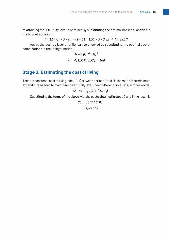
115Index numbers and their relationship with the economy Annexes
of attaining the 100 utility level is obtained by substituting the optimal basket quantities in the budget equation:
I 11 Q 5 Q I 11 1.51 5 3.32 I 33.171x
1y= + = + =& &$ $ $ $
Again, the desired level of utility can be checked by substituting the optimal basket combinations in the utility function:
U 4(Q ) (Q )1x 2
1y 2=
U 4(1.51)2 (3.32)2 = 100=
Stage 3: Estimating the cost of living
The true consumer cost of living index (CLI) between periods 0 and 1 is the ratio of the minimum expenditure needed to maintain a given utility level under different price sets, in other words:
CLI1 = C (U0, P1) / C (U0, P0)
Substituting the terms of the above with the costs obtained in steps 0 and 1, the result is
CLI1 = 33.17 / 31.62
CLI1 = 4.9%

116 Economic Commission for Latin America and the Caribbean (ECLAC)Annexes
Annex A4
Constant elasticity of substitution (CES) production function: output maximization, cost minimization and price indices
This annex provides a comprehensive analysis of the output maximization and cost minimization processes, and their connection to price indices. The following steps can be applied to any type of production function (production theory) or utility function (consumer theory). In this case, they will apply to a constant elasticity of substitution production function.
1. Definition of the function
Theconstantelasticityofsubstitutionfunctionisdefinedas
f (K,L) Q A ( K L )* * v/p= = +a b --p -p
Where:
K: capital input
L: labour input
Q: output quantity
A: technology parameter
α: parameter representing the ratio of capital K to total income
β: parameter representing the ratio of labour L to total income (α + β = 1)
ρ: parameter representing the Allen partial elasticity of substitution σKL, where ρ = (σ-1)/σ
ν: parameter representing economy of scale or degree of homotheticity of the function, such that ν = 1 implies constant returns to scale (a homogeneous function of degree 1); ν< 1 means decreasing returns to scale (a homogeneous function of degree n < 1), and ν >1 indicates increasing returns to scale (a homogeneous function of degree n > 1)
Assume the following values for the CES function:
Q = 1 * (0.3 K -0.17647 + 0.7 L -0.17647) - ( 1 / 0.17647)
Consequently, A = 1, α= 0.3, β = 0.7 (note that the condition α + β= 1 isverified), ρ = 0.17647 (so σKL= 0.85) andν = 1. Accordingly, the function displays constant returns to scale and is homogeneous of degree 1.
The production function Q = f(K, L) is called the direct production function, since it directly relates the factors of production to the quantities (Q) produced, and implicitly includes the underlying technology in the production process. The arguments of the Q function are the elements that make up the value added of production. If intermediate consumption is included, the Q will also cover the products used as inputs in production.
117Index numbers and their relationship with the economy Annexes
2. Budget constraint
The budget constraint is given by the following equation
R = PK . K + PL . L
where:
A: budget constraint
PK: capital factor price
K: capital input quantity
PL: labour factor price
L: labour input quantity
Once the production function Q=f(K,L) and the budget constraint R have been defined,twooptimizationprocessescanbeperformed:outputmaximizationandcostminimization. Both processes make it possible to determine the optimal factor demand needed to maximize production at minimum cost. The output maximization process is called the primal analysis, and the cost minimization process is the dual. By performing both processes, it will be seen that the amounts demanded of the factors coincide; in other words, the same result is reached, either by maximizing production or by minimizing costs.
3. Maximizing production: direct and indirect production function
The primal problem entails selecting optimal levels of demand for factors K and L, so as to obtain a maximum level of output Q, given the existing price vector (PK, PL) and a budget constraint R. Analytically, it can be expressed as follows:
max Q (K,L), subject to R=K.PK0+L.PL0
where:
Q (K,L) is production function Q, and
R = K.PK0 + L.PL0 is the budget line that results from multiplying the quantities of the inputs, K and L, by their prices in period 0, namely PK0 and PL0.
The solution to the problem of maximizing Q(K, L) requires determining the “Marshallian” or “ordinary” quantities of capital and labour demanded (Km and Lm). The mathematical solution is found by using the Lagrange multiplier method. Along with the Marshallian factordemands,anequationwillalsobeobtainedthatdefinesthe indirectproductionfunction, G(R, PK, PL), in which the quantity produced no longer depends on the quantities of the productive factors, but on the budget constraint and the factor prices. This function maximizes the amount produced from an economic perspective, taking costs into account. The producer will demand factors in quantities that make it possible to maximize the output of Q, given the available budget and prevailing factor prices.

118 Economic Commission for Latin America and the Caribbean (ECLAC)Annexes
Given the factor prices prevailing in period 0, namely PK0 = 10 and PL0 = 5, and an availablebudgetofUS$ 1,178.4forfactorcosts,theproblemistodeterminethefactorquantities (Km and Lm) that make it possible maximize production Q.
This can be expressed as
max Q 1.(0.3 . K 0.7 . L )0.176470
0.17647 (0.176471 )= + -- - subject to R = 10 . K + 5.L = 1,178 . 4
Applying Lagrange multipliers gives:
γ(Q, K, L, λ) = f (K, L) + λ . (R - pK . K + pL . L)
= (α K -ρ + β L -ρ) - (ν / ρ) + λ . (R - pK . K + pL).
Thefirst-orderconditionsareasfollows:
(i) γK = fK - λ . pK = 0, where fK = α Kρ-1 (α Kρ + β Lρ) (1-ρ / ρ) - λ pK = 0
(ii) γL = fL - λ . pL = 0, where fL = β Lρ-1 (α Kρ + β Lρ) (1-ρ / ρ) - λ pL = 0
(iii) γΛ = I - pK . K - pL . L = 0
Equations (i) and (ii) above can be combined to give:
(iv) pK / pL = f K / f L
pK / pL = f K / f L = (α / β) . (L / K) (ρ − 1)
Solving for L and K gives:
(v) L = K * (pK . β/(pL . α))(1/(ρ − 1))
K = L * (pL . α/(pK . β))(1/(ρ − 1))
If K and L are substituted in the budget line R according to the values of (v):
R = pK . K + pL . K . (pK . β/(pL . α))(1/(ρ-1)) = R = pK . K + pL . K . (pK . β/(pL . α)) -σ
R = K . [pK + pL . (pK . β/(pL . α))(1/(ρ − 1))] = R = K . [pK + pL . (pK . β/(pL . α))-σ]
Solving for K and L, gives the Marshallian quantities demanded, Km and Lm:
Km = R/[pK + pL . (pK . β/(pL . α ))-σ]
Km = (α . pL)σ . R/(ασ . pK . pLσ + βσ . pL . pKσ)
Lm = R/[pL + pK . (pL . α/(pK . β))-σ]
Lm = (β . pK) σ . R/(bσ . pL . pKσ + aσ . pL . pKσ)

119Index numbers and their relationship with the economy Annexes
As can be seen, the Marshallian demand quantities have been expressed in terms of parameters, prices and budget constraints.
If the values of the parameters given by the CES production function are incorporated into the Marshallian demands, along with the period-0 factor prices (PK0 = 10 and PL0 = 5) and themonetaryvalueofthebudgetconstraint(US$ 1,178.4),thequantitiesoffactorsK and L demanded can be calculated as K=41.32 and L=153.04.
If these quantities are substituted into in the CES direct production function, Q = f(K, L), the value of the function indicates the optimal quantity to be produced (100 units of Q):
Q = 1 * (0.3 . 41.32-0.17647 + 0.7 . 153.04-0.17647)- ( 1 / 0.17647) = 100
Inotherwords,withabudgetofUS$ 1,178.4,thepricesprevailingattime0(PK0 = 10 and PL0 = 5) and the technology given by the constant CES direct production function, the maximum attainable output is 100 units of Q, using 41.32 units of factor K and 153.04 units of L.
The indirect production function is obtained by substituting the Marshallian demands in the objective function, the direct production function:
Q = f (K,L) = A . (α . K-ρ + β L-ρ )-ν/ρ = A . (α . Km-ρ + β Lm-ρ)-ν/ρ
Through successive operations, the indirect production function G can be obtained as:
G = f (R, PK, PL)
= R . [ασ * PL σ-1 + βσ * PK σ-1] 1 /(σ-1) / (PK * PL)
= R . [ασ * PK 1-σ + βσ * PL 1-σ]-1 /(1-σ)
This function makes it possible to calculate maximum output levels Q, for different K and L factor prices and the budget available to remunerate the factors used in the production process.
The Marshallian demands can also be obtained from Roy’s identity:
Km = - GpK / GR
Lm = - GpL / GR
where:
GpK: derivative of the indirect production function G with respect to factor K prices
GpL: derivative of the indirect production function G with respect to factor L prices
GR: derivative of the indirect production function G with respect to budget line R
Calculating the derivatives gives the following:
GpK = 1/(1-σ) . (ασ . PK1-σ + βσ . PL
1-σ)-(1 + 1/(1-σ)) * R . (1-σ) . ασ . PK(1-σ)-1
GpL = 1/(1-σ) . (ασ . PK1-σ + βσ . PL
1-σ)-(1 + 1/(1-σ)) . R * (1-σ) . βσ . PL(1-σ)-1

120 Economic Commission for Latin America and the Caribbean (ECLAC)Annexes
Roy’s identity makes it possible to obtain the Marshallian demands from a single equation, in a much simpler way than the traditional estimation in which a series of equations have to be solved using the Lagrange multiplier method. Given any factor price and any budget, it is possible to obtain the factor quantity needed to maximize production.
A possible economic explanation for Roy’s identity would be as follows. The Marshallian quantities demanded (for example, Km) are equal to a quotient of partial derivatives of the indirect production function G, with a negative sign (-GpK / GR). The partial derivative GpK indicates the effect on production of a unit change in the price of the capital factor Pk. The partial derivative GR indicates how output is changed by a one-unit change in the budget line R. The partial derivative GpK would represent the way in which Pk is transformed into G units produced, and GR the way in which the budget constraint R is transformed into G units produced. Since GR is in the denominator of Roy’s identity, it is in fact the inverse of that derivative. It therefore means the way in which the budget line R is altered by a variation in production G; or, equivalently, it expresses the change that occurs in production expressed in the same units as the budget R, namely monetary values. Inshort,firstly,itisknownhowmuchtheoutputG varies in response to a change in price Pk (GpK) and, subsequently, that output G is converted into R, that is, into monetary values (GR
-1). In short, the multiplication GpK. GR
-1 expresses in monetary terms how a change in Pk affects production. Since production expressed in monetary values is the cost of production, Roy’s identity can be interpreted as the effect on the cost of production of a one unit increase in the factor price Pk. In the example given, if Roy’s identity yields a value of 41.32 for K, it means that a one unit change in Pk generates a change of 41.32 units in the cost of production. In other words, Roy’s identity makes it possible to match the quantities demanded Km with the cost, in terms of production, of a variation in its unit price.
Source: Prepared by the authors.
GR = [ασ . PK1-σ + βσ . PL
1-σ]-1/(1-σ)
ItcanbeconfirmedthatthesamevaluesoftheMarshalliandemandfunctionsareobtained: K=41.32 and L=153.04.
4. Minimization of production costs
The minimization problem (the dual) entails choosing the optimal quantities of demand for factors K and L, such that costs are minimized, taking into account the existing price vector andthespecificlevelofproductiontobeattained.Itcanbeformulatedasfollows:
min R= K.PK0 + L.PL0, subject to Q (K,L)
Solving the minimization problem involves calculating the “Hicksian” or “compensated” factor demands (Kh and Lh), for which the mathematical solution is obtained through the Lagrange multiplier method.
■ Box A4.1 Roy’s identity

121Index numbers and their relationship with the economy Annexes
Hicksian demand quantities (Kh and Lh) are a function of prices (PK and PL) and the production level Q, such that Kh = f(PK,Q) and Lh = f(PL,Q).
Given the factor prices prevailing in period 0, PK0 = 10 and PL0 = 5, and the desired production level of 100 units of Q, the problem involves determining the factor quantities (Kh and Lh) that make it possible to minimize costs.
In other words:
Applying Lagrange multipliers gives:
(Q, K, L, ) = R + * (Q - f (K,L)) = PK * K + PL * L + * (Q - f (K,L))
Thefirstorderconditionsare:
(i) γK = PK - λ * fK = 0, where fK = PK - λ . α K ρ-1 . (α Kρ + β Lρ)(1-ρ / ρ) = 0
(ii) γL = PL - λ * fL = 0, where fL = PL - λ . β Lρ-1 . (α Kρ + β Lρ)(1-ρ / ρ) = 0
(iii) γΛ = Q - fKL = 0
Combining (i) and (ii) gives:
(iv) PK/PL = f K/f L = (α/β) . (K/L) (1 + ρ)
The latter expression is the marginal rate of substitution between factors K and L (see section 5 of this annex), where K and L can be solved as:
(v) L = K . (PK . β/(PL . α ))(1/(1+ρ))
K = L . (PL . α/(PK . β ))(1/(ρ − 1))
Substituting for L in the direct production function Q = A.(α.K-ρ + β.L-ρ )-ν/ρ gives:
Q = A * {α∗K-ρ + β * [K * (pK * β/(pL * α))(1/(1+ρ))]-p]-ν/p}
Solving for K in this function gives the Hicksian or compensated demand function Kh:
K = (Q/A)1/ν [α + β . (pK . β/(pL . α))(-ρ/(1+ρ))](1/ρ)
Kh = (Q/A)1/ν . (α/pK)(1/(1+ρ)) . [α(1/1+ρ)) . pK(ρ/(1+ρ)) + β(1/(1+ρ)) . pL(ρ/(1+ρ))](1/ρ)
Similarly, solving for L gives the Hicksian demand Lh:
Lh = (Q/A)1/ν . (β/pL)(1/(1+ρ)) . [β(1/1+ρ)) . pL(ρ/(1+ρ)) + α(1/(1+ρ)) . pK(ρ/(1+ρ))](1/ρ)
As can be seen, the Hicksian demands are obtained from the parameters, factor prices and the quantities to be produced.
Substituting the values of the parameters given by the CES production function into the Hicksian demands, along with the prices prevailing in period 0 (PK0 = 10 and PL0 = 5) and the number of units of Q to be produced (100), makes it possible to calculate the quantities

122 Economic Commission for Latin America and the Caribbean (ECLAC)Annexes
demanded of the factors K and L: K=41.32 and L=153.04. As can be seen, these quantities are the same as the Marshallian demand quantities obtained in Chapter III, so Kh = Km and Lh = Lm.
If in the objective function, the budget line, K and L are replaced by the Hicksian demands, Kh and Lh, and the relevant operations are performed, the following minimum cost function e is obtained:
e = Q . [ασ . pK1-σ + βσ . pL1-σ]1 /(1-σ) = Q . C(1,P)
where the function C(1,P) is the unit cost of production. The minimum cost is thus obtained by multiplying the quantities Q to be produced by the unit cost C(1,P). This is a minimum cost because it has been calculated from the cost minimization process.
Substituting the period-0 prices (PK0 = 10 and PL0 = 5) and the parameters of the example of the CES function gives C(1,P)=US$ 11.78.Multiplyingthedesiredoutputof100 units of QbyUS$ 11.78givesUS$ 1,178.4,whichistheamountneededtopayforthe41.32 units of factor K,atapriceofUS$ 10,andthe153.04unitsofL,atapriceofUS$ 5.TheUS$ 1,178.4representsthevalueofthebudgetconstraint imposedontheoutputmaximization process.
Oncetheunitcostofproductionfunctionhasbeenobtained,itisverysimpletofindthe minimum cost for any desired level of output. For example, for an output of 1,500 units of Q,multiplyingthatvaluebyUS$ 11,784givesabudgetofUS$ 17,675.7.1 It is also possible to findthenecessaryfactorquantities(orHicksiandemands)Kh = 619.8 and Lh = 2,295.6 units.
In the unit cost function, the average cost and minimum cost are the same, since, once the cost minimization process has been completed, e = R.
Replacing e by R in the minimum cost function e = Q . C(1,P), , gives:
R = Q . C(1,P)
Replacing Q (the direct production function) by G (the indirect production function), gives:
R = G . C(1,P)So G = R/C(1,P) = R . C(1,P)
-1
In other words, the indirect production function G is the budget line R multiplied by the inverse of the unit cost function C(1,P)
-1,whichisanotherwayofdefiningtheindirectproduction function G obtained in the (primal) output maximization analysis.
Differentiating the minimum cost function e = G . [ασ . PK1-σ + βσ . PL
1-σ]1/(1-σ) with respect to PK, gives the following derivative:
ePK = G * ασ∗ pK-σ* (aσ∗ pK(1-σ) + βσ* pL) (σ/1-σ)
1 Assumingconstantreturnstoscale,asspecifiedinthisexample.

123Index numbers and their relationship with the economy Annexes
According to Shephard’s Lemma, this expression represents the value of the Hicksian demand Kh, so:
Kh = G * ασ ∗ pK-σ * (ασ ∗ pK(1-σ) + βσ * pL)(σ/1-σ) Similarly:
Lh = ePL = G * βσ ∗ pL-σ * (ασ ∗ pK(1-σ) + βσ * pL)(σ/1-σ)
This is another way of obtaining Hicksian factor demands: the quantity demanded of a factor is the variation in cost resulting from a change in its price, holding output constant (since the latter is optimal).
Shephard’s Lemma makes it possible to obtain Hicksian demand functions from the derivatives of the expenditure function. As with Roy’s Identity, Shepard’s Lemma obviates the need for a more complex procedure (in this case, solving the expenditure minimization problem) by solving a single equation.
■ Box A4.2 Shephard’s Lemma
The economic interpretation of Shephard’s lemma is straightforward: when the price of a factor (PL for example) rises by one unit, the unit cost of production increases according to the quantities demanded of that factor (Lh).
Source: Prepared by the authors.
5. Elasticity of substitution between factors
The factor prices prevailing in period 0 (PK0 = 10; PL0 = 5) may change in period 1. For example, if PKinperiod1risestoUS$ 11(PK1=11) and PL1remainsunchangedatUS$ 5(PL1=5), the relative factor price increases by 10% between periods 0 and 1: the relative price PK0/PL0 = 10/5 = 2 would become PK1/PL1 = 11/5 = 2.2.
In response to such a change, rational and optimizing behaviour leads the producer to increase the use of the factor whose relative price has fallen (L) and to decrease the use of the factor whose relative price has risen (K). Obviously, for this to be viable, it is assumed that the available technology allows the producer to alter the intensity of factor use, through an economic decision that allows the level of production to be kept constant at 100 (Q0=Q1=100), at minimum cost. Following a 10% increase in the relative price, there is a wide range of possible combinations of K and L, but there will only be one that guarantees that the level of production can be maintained at minimum cost. The problem is to determine the new levels of K and L that keep production at 100 and minimize costs in response to a change in the relative factor price PK1/PL1 = 11/5 = 2.2. In other words, what are the new optimum demands for factors K and L following a 10% increase in the price of PK relative to PL?

124 Economic Commission for Latin America and the Caribbean (ECLAC)Annexes
The answer to this question depends on the elasticity of substitution between the two factors, which is derived below for the CES case. As noted above, in the CES function this elasticity is denoted by σ, which, in this example, takes the value σ= 0.85. This means that, following a 10% change in the price PK relative to PL, the producer will have to increase the quantity demanded of L relative to K by 8.5% (10% x 0.85) in order to keep the level of production at 100 units at a minimum cost. As this is a CES function, the elasticity of substitution is constant at any output level Q.
Calculating the value of the elasticity of substitution is based on the equation presented in section 4(iv) on minimizing production costs, which was as follows:
PK/PL = f K/f L = (α/β) . (K/L) (1 + ρ)
Rearranging gives:
(i) L/K = [(β/α) * (PK/PL)](1/(1+ρ)) = (β/α)1/(1+ρ) * (PK/PL)1/(1+ρ))
Differentiating with respect to PK / PL, gives:
(ii) d (L/K)/d (PK/PL) = (1/(1+ ρ)) * (β/α)1/(1+ρ) * (PK/PL)(1/(1+ρ)-1)
The elasticity of substitution σ measures how a percentage change in relative prices affects the quantities demanded; in this case, how PK/PL affects L/K, in other words:
(iii) α= percentage change in L/K / percentage change in PK / PL
= (d (L/K)/(L/K))/(d(PK/PL)/(PK/PL))
= (d (L/K)/d(PK/PL)) * ((PK/PL)/(L/K))
In (ii), replacing (d (L/K)/d(PK/PL)) by (1/(1+ ρ)) * (β/α)1/(1+ρ) * (PK/PL) (1/(1+ρ)-1), gives:
σ = [(1/(1+ ρ)) * (β/α)1/(1+ρ) * (PK/PL)(1/(1+ρ)-1) ] * ((PK/PL)/(L/K))
In (i) replacing (L/K) with (β/α)1/(1+ρ) * (PK/PL)1/(1+ρ), gives
σ = [(1/(1+ρ)) * (β/α)1/(1+ρ) * (PK/PL)(1/(1+ρ)-1)] * [(PK/PL)/((β / α)1/(1+ρ) * (PK/PL)1/(1+ρ))]
Eliminating (β/α) 1/(1+ρ) gives
σ = [(1/(1+ ρ)) * (PK/PL)(1/(1+ρ)-1) * [(PK/PL)]/(PK/PL)1/(1+ρ)) = [(1/(1+ ρ)) * (PK/PL)1/(1+ρ)]/(PK/PL)1/(1+ρ))
Furthersimplificationshowsthat,intheCESfunction,σ = 1/(1+ ρ).
Substituting the latter expression in (i) gives:
L/K = (β/α)1/(1+ρ) * (PK/PL)1/(1+ρ))
= (β/α)σ * (PK/PL)σ

125Index numbers and their relationship with the economy Annexes
Accordingly, given the parameters α, β and σ the prices PK and PL, the value of the elasticity of substitution can be checked. Assuming the situation in period 0, with prices (PK0 = 10 and PL0 = 5) and optimum quantities (K=41.32 and L=153.04), then:
L/K = 153.04/41.32 = 3.70 and
(β/α)σ * (PK/PL)σ = (0.70/0.30)0.85 * (10/5)0.85 = 3.70
If the price ratio in situation 0 (PK/PL = 10/5 = 2) increases by 10% to 2.2, due to the 10% increase in PK (PK/PL = 11/5 = 2.2), then (β/α)σ * (PK/PL)σ= (0.70/0.30)0.85 * (11/5)0.85= 4.02, is recalculated,sothat4.02/3.70representsanincreaseof8.44%,reflectingtheriseinL/K caused by a 10% rise in PK. The value of 8.44% coincides with the value of the elasticity of substitution σ =0.85andwiththenewoptimumpointofuseofthefactorsforperiod 1.If the relative quantities of period 1 (L/K =157.47/39.21=4.016) are compared with those of period 0 (L/K =153.04/41.32=3.704), the use of L increases by 8.44% relative to K.

126 Economic Commission for Latin America and the Caribbean (ECLAC)Annexes
Annex A5
The problem of drift
This example, taken from the International Monetary Fund’s Quarterly National Accounts Manual: concepts, data sources and compilation,2 shows a situation where prices and quantities of two products (A and B) are the same in the initial period (quarter 1)3andinthefinalperiod(quarter4).Ascanbeseen,theLaspeyres,PaascheandFisherfixed-basevolumeindicesgive a value of 100 for both periods (as expected), while the Laspeyres, Paasche and Fisher chain-linked indices report a value of 100 in the initial period, but a different value in the finalperiod.
■ Table A5.1 Frequency of chaining and problem of “drift” in the case of price and quantity fluctuations
Observation/Quarter Quarter 1 Quarter 2 Quarter 3 Quarter 4
Price item A (pA) 2 3 4 2
Price item B (pB) 5 4 2 5
Quantities item A (qAt) 50 40 60 50
Quantities item B (qBt) 60 70 30 60
Total value (Vt) 400 400 300 400
Volume indices q1 q2 q3 q4
Fixed-base Laspeyres (Q1-based) 100.0 107.5 67.5 100.0
Fixed-base Paasche (Q1-based) 100.0 102.6 93.8 100.0
Fixed-base Fisher (Q1-based) 100.0 105.0 79.6 100.0
Quarterly chain-linked Laspeyres 100.0 107.5 80.6 86.0
Quarterly chain-linked Paasche 100.0 102.6 102.6 151.9
Quarterly chain-linked Fisher 100.0 105.0 90.9 114.3
Source: Prepared by the authors on the basis of A. Bloem, R. Dippelsman and N. Maehle, Quarterly National Accounts Manual: Concepts, Data, Sources and Compilation, Washington, D.C., International Monetary Fund (IMF), 2001, chapter 9, p.156.
2 See A. Bloem, R. Dippelsman and N. Maehle, Quarterly National Accounts Manual: Concepts, Data, Sources and Compilation,Washington,D.C.,InternationalMonetaryFund(IMF),2001[online]https://www.imf.org/external/pubs/ft/qna/2000/textbook/index.htm.
3 In the example, quarters are used as periods, but the example can also be extended to annual periods, with the same values.

127Index numbers and their relationship with the economy Annexes
Annex A6
Practical exercises: annual chain-linked volume measures
This annex includes three exercises to apply the chain-linked volume index calculation formula.
Tables A6.1 and A6.2 present the GDP series of a country from 2001 to 2015, at current and constant 2005 prices, respectively, disaggregated into production sectors.
■ Table A6.1 Gross value added by sector and GDP
(Thousands of current pesos)
Sectors Agriculture Mining Manufacturing Information technology Total GDP
2001 150 300 370 200 1 020
2002 150 320 379 190 1 039
2003 160 340 386 180 1 066
2004 170 360 393 170 1 093
2005 180 380 400 160 1 120
2006 190 400 405 150 1 145
2007 200 420 410 140 1 170
2008 150 370 375 120 1 015
2009 160 390 383 110 1 043
2010 170 410 390 100 1 070
2011 180 430 397 90 1 097
2012 190 450 404 80 1 124
2013 200 470 411 70 1 151
2014 210 490 418 60 1 178
2015 220 510 425 50 1 205
Source: Prepared by the authors.
■ Table A6.2 Gross value added by sector and GDP
(Thousands of pesos at constant 2005 prices)
Sectors Agriculture Mining Manufacturing Information technology Total GDP
2001 160 340 380 80 960
2002 165 350 385 100 1 000
2003 170 360 390 120 1 040
2004 175 370 395 140 1 080
2005 180 380 400 160 1 120
2006 185 390 405 180 1 160
2007 190 400 410 200 1 200
2008 180 350 380 190 1 100

128 Economic Commission for Latin America and the Caribbean (ECLAC)Annexes
Sectors Agriculture Mining Manufacturing Information technology Total GDP
2009 185 360 385 210 1 140
2010 190 370 390 230 1 180
2011 195 380 395 250 1 220
2012 200 390 400 270 1 260
2013 205 400 405 290 1 300
2014 210 410 410 310 1 340
2015 215 420 415 330 1 380
Source: Prepared by the authors.
The aim is to calculate the chain-linked index, with 2005 as the reference year, as well as GDP expressed as a chain-volume measure in monetary terms referenced to 2005.
Solution
Step 1: Calculate the elementary indices (2005=100).
■ Table A6.3 Elementary volume indices
(Base 2005=100)
Sectors Agriculture Mining Manufacturing Information technology
2001 88.89 89.47 95.00 50.00
2002 91.67 92.11 96.25 62.50
2003 94.44 94.74 97.50 75.00
2004 97.22 97.37 98.75 87.50
2005 100.00 100.00 100.00 100.00
2006 102.78 102.63 101.25 112.50
2007 105.56 105.26 102.50 125.00
2008 100.00 92.11 95.00 118.75
2009 102.78 94.74 96.25 131.25
2010 105.56 97.37 97.50 143.75
2011 108.33 100.00 98.75 156.25
2012 111.11 102.63 100.00 168.75
2013 113.89 105.26 101.25 181.25
2014 116.67 107.89 102.50 193.75
2015 119.44 110.53 103.75 206.25
Source: Prepared by the authors.
Table A6.2 (concluded)

129Index numbers and their relationship with the economy Annexes
Step 2: Calculate the annual weights at current prices.
■ Table A6.4 Annual weights at current prices
Sectors Agriculture Mining Manufacturing Information technology Total
2001 0.1471 0.2941 0.3627 0.1961 1.0000
2002 0.1444 0.3080 0.3648 0.1829 1.0000
2003 0.1501 0.3189 0.3621 0.1689 1.0000
2004 0.1555 0.3294 0.3596 0.1555 1.0000
2005 0.1607 0.3393 0.3571 0.1429 1.0000
2006 0.1659 0.3493 0.3537 0.1310 1.0000
2007 0.1709 0.3590 0.3504 0.1197 1.0000
2008 0.1478 0.3645 0.3695 0.1182 1.0000
2009 0.1534 0.3739 0.3672 0.1055 1.0000
2010 0.1589 0.3832 0.3645 0.0935 1.0000
2011 0.1641 0.3920 0.3619 0.0820 1.0000
2012 0.1690 0.4004 0.3594 0.0712 1.0000
2013 0.1738 0.4083 0.3571 0.0608 1.0000
2014 0.1783 0.4160 0.3548 0.0509 1.0000
2015 0.1826 0.4232 0.3527 0.0415 1.0000
Source: Prepared by the authors.
Step 3: Calculate the elementary volume indices (previous year=100)
■ Table A6.5 Elementary volume indices(Previous year = 100)
Sectors Agriculture Mining Manufacturing Information technology
2001
2002 103.13 102.94 101.32 125.00
2003 103.03 102.86 101.30 120.00
2004 102.94 102.78 101.28 116.67
2005 102.86 102.70 101.27 114.29
2006 102.78 102.63 101.25 112.50
2007 102.70 102.56 101.23 111.11
2008 94.74 87.50 92.68 95.00
2009 102.78 102.86 101.32 110.53
2010 102.70 102.78 101.30 109.52
2011 102.63 102.70 101.28 108.70
2012 102.56 102.63 101.27 108.00
2013 102.50 102.56 101.25 107.41
2014 102.44 102.50 101.23 106.90
2015 102.38 102.44 101.22 106.45
Source: Prepared by the authors.

130 Economic Commission for Latin America and the Caribbean (ECLAC)Annexes
Step 4: Calculate the links by multiplying the annual weights by the volume indices (previous year=100).
■ Table A6.6 Links
Sectors Agriculture Mining Manufacturing Information technology Total
2001
2002 15.17 30.28 36.75 24.51 106.70
2003 14.87 31.68 36.95 21.94 105.45
2004 15.45 32.78 36.67 19.70 104.61
2005 16.00 33.83 36.41 17.78 104.01
2006 16.52 34.82 36.16 16.07 103.57
2007 17.04 35.83 35.81 14.56 103.24
2008 16.19 31.41 32.48 11.37 91.45
2009 15.19 37.49 37.43 13.07 103.18
2010 15.75 38.43 37.20 11.55 102.93
2011 16.31 39.35 36.92 10.16 102.73
2012 16.83 40.23 36.65 8.86 102.57
2013 17.33 41.06 36.39 7.64 102.43
2014 17.80 41.85 36.15 6.50 102.30
2015 18.25 42.61 35.92 5.42 102.20
Source: Prepared by the authors.
Step 5: Calculate the chain index (reference year: 2005) and GDP as a chain-volume measure in monetary terms referenced to 2005.
■ Table A6.7 Chain-linked index and GDP as a chain-volume measure in monetary terms referenced to 2005
YearChain-linked index
(Reference year: 2005)
GDP(Chain-volume measure in monetary
terms referenced to 2005)Percentage change
2001 81.68 915
2002 87.16 976 6.7
2003 91.91 1 029 5.4
2004 96.14 1 077 4.6
2005 100.00 1 120 4.0
2006 103.57 1 160 3.6
2007 106.92 1 198 3.2
2008 97.78 1 095 -8.5
2009 100.89 1 130 3.2
2010 103.86 1 163 2.9

131Index numbers and their relationship with the economy Annexes
YearChain-linked index
(Reference year: 2005)
GDP(Chain-volume measure in monetary
terms referenced to 2005)Percentage change
2011 106.69 1 195 2.7
2012 109.43 1 226 2.6
2013 112.09 1 255 2.4
2014 114.67 1 284 2.3
2015 117.19 1 313 2.2
Source: Prepared by the authors.
Table A6.8 calculates GDP at constant 2005 prices, in order to compare the results of the annual rates of change and the statistical discrepancy due to non-additivity in the chain-linkedfigures.4
■ Table A6.8 GDP at constant 2005 prices and statistical discrepancy due to non-additivity
Year Fixed base Percentage change, fixed base Statistical discrepancy
2001 960 -45
2002 1 000 4.2 -24
2003 1 040 4.0 -11
2004 1 080 3.8 -3
2005 1 120 3.7 -
2006 1 160 3.6 -
2007 1 200 3.4 -2
2008 1 100 -8.3 -5
2009 1 140 3.6 -10
2010 1 180 3.5 -17
2011 1 220 3.4 -25
2012 1 260 3.3 -34
2013 1 300 3.2 -45
2014 1 340 3.1 -56
2015 1 380 3.0 -67
Source: Prepared by the authors.Note: The highlighted figure indicates that the rate of change of the first consecutive year (2006) with respect to
the base year (2005) coincides with the rate of change of the chain-linked index presented in table A6.7.
Tables A6.9 and A6.10 present the previous year’s GDP, but measured from the expenditure side. The aim is to calculate the chain-linked index, taking 2005 as the reference year, and GDP according to 2005 chain-linked currency.
4 ThisisthedifferencebetweentheGDPfiguresinchain-linkedcurrencyof2005andGDPatconstant2005prices.
Table A6.7 (concluded)

132 Economic Commission for Latin America and the Caribbean (ECLAC)Annexes
■ Table A6.9 Gross domestic product by expenditure component
(Thousands of current pesos)
Sectors Consumption Capital formation Exports Imports Total GDP
2001 650 300 400 -330 1 020
2002 670 305 405 -341 1 039
2003 690 310 400 -334 1 066
2004 710 320 405 -342 1 093
2005 730 325 410 -345 1 120
2006 750 330 415 -350 1 145
2007 770 335 420 -355 1 170
2008 760 280 410 -435 1 015
2009 780 295 415 -447 1 043
2010 800 300 420 -450 1 070
2011 820 305 425 -453 1 097
2012 840 315 427 -458 1 124
2013 860 320 432 -461 1 151
2014 880 325 437 -464 1 178
2015 900 330 442 -467 1 205
Source: Prepared by the authors.
■ Table A6.10 Gross domestic product by expenditure component
(Thousands of pesos at constant 2005 prices)
Sectors Consumption Capital formation Exports Imports Total GDP
2001 710 285 390 -425 960
2002 715 295 395 -405 1 000
2003 720 305 400 -385 1 040
2004 725 315 405 -365 1 080
2005 730 325 410 -345 1 120
2006 735 335 415 -325 1 160
2007 740 345 430 -315 1 200
2008 730 295 410 -335 1 100
2009 735 305 420 -320 1 140
2010 740 315 425 -300 1 180
2011 745 325 430 -280 1 220
2012 750 335 435 -260 1 260
2013 755 345 440 -240 1 300
2014 760 355 445 -220 1 340
2015 765 365 450 -200 1 380
Source: Prepared by the authors.

133Index numbers and their relationship with the economy Annexes
This exercise is completed by repeating the steps of the previous exercise. The results are shown in table A6.11.
■ Table A6.11 Chain-linked volume index (reference year: 2005) and GDP as a chain-volume measure in monetary terms referenced to 2005, measured on the expenditure side
YearChain-linked
index(reference year: 2005)
GDP expenditure
approach(monetary-term chain-
volume measure
referenced to 2005)
Percentage change,
expenditure approach
Production approach
(monetary-term chain-
volume measure
referenced to 2005)
Percentage change,
production approach
Difference (expenditure approach minus
production approach)(monetary-term
chain-volume measure referenced to 2005)
2001 87.05 975 915 60
2002 90.10 1 009 3.5 976 6.7 33
2003 93.31 1 045 3.6 1 029 5.4 16
2004 96.57 1 082 3.5 1 077 4.6 5
2005 100.00 1 120 3.5 1 120 4.0 -
2006 103.57 1 160 3.6 1 160 3.6 -
2007 107.25 1 201 3.6 1 198 3.2 4
2008 97.99 1 098 -8.6 1 095 -8.5 2
2009 102.26 1 145 4.4 1 130 3.2 15
2010 106.95 1 198 4.6 1 163 2.9 35
2011 111.93 1 254 4.7 1 195 2.7 59
2012 117.26 1 313 4.8 1 226 2.6 88
2013 123.01 1 378 4.9 1 255 2.4 122
2014 129.24 1 448 5.1 1 284 2.3 163
2015 136.05 1 524 5.3 1 313 2.2 211
Source: Prepared by the authors.
The GDP results from the production approach obtained in year 1 have also been included for comparison purposes.
Exercise 3. Tables A6.12 and A6.13 present the GDP series for year 1, disaggregated down by sector, with a further disaggregation of the manufacturing sector.
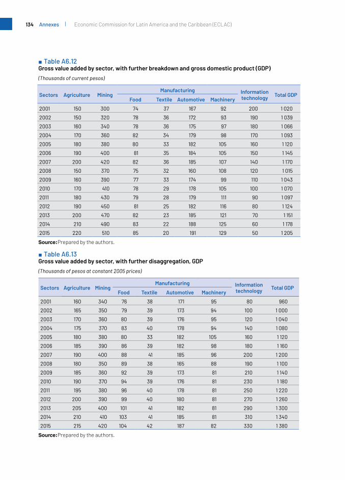
134 Economic Commission for Latin America and the Caribbean (ECLAC)Annexes
■ Table A6.12 Gross value added by sector, with further breakdown and gross domestic product (GDP)
(Thousands of current pesos)
Sectors Agriculture MiningManufacturing Information
technology Total GDPFood Textile Automotive Machinery
2001 150 300 74 37 167 92 200 1 020
2002 150 320 78 36 172 93 190 1 039
2003 160 340 78 36 175 97 180 1 066
2004 170 360 82 34 179 98 170 1 093
2005 180 380 80 33 182 105 160 1 120
2006 190 400 81 35 184 105 150 1 145
2007 200 420 82 36 185 107 140 1 170
2008 150 370 75 32 160 108 120 1 015
2009 160 390 77 33 174 99 110 1 043
2010 170 410 78 29 178 105 100 1 070
2011 180 430 79 28 179 111 90 1 097
2012 190 450 81 25 182 116 80 1 124
2013 200 470 82 23 185 121 70 1 151
2014 210 490 83 22 188 125 60 1 178
2015 220 510 85 20 191 129 50 1 205
Source: Prepared by the authors.
■ Table A6.13 Gross value added by sector, with further disaggregation, GDP
(Thousands of pesos at constant 2005 prices)
Sectors Agriculture MiningManufacturing Information
technology Total GDPFood Textile Automotive Machinery
2001 160 340 76 38 171 95 80 960
2002 165 350 79 39 173 94 100 1 000
2003 170 360 80 39 176 95 120 1 040
2004 175 370 83 40 178 94 140 1 080
2005 180 380 80 33 182 105 160 1 120
2006 185 390 86 39 182 98 180 1 160
2007 190 400 88 41 185 96 200 1 200
2008 180 350 89 38 165 88 190 1 100
2009 185 360 92 39 173 81 210 1 140
2010 190 370 94 39 176 81 230 1 180
2011 195 380 96 40 178 81 250 1 220
2012 200 390 99 40 180 81 270 1 260
2013 205 400 101 41 182 81 290 1 300
2014 210 410 103 41 185 81 310 1 340
2015 215 420 104 42 187 82 330 1 380
Source: Prepared by the authors.

135Index numbers and their relationship with the economy Annexes
The exercise is completed by repeating the steps of the previous exercises. Table A6.14 shows the results and the comparison with the results of exercise 1.
■ Table A6.14 Chain-linked volume index (reference year: 2005) and GDP according to the 2005 monetary chain, with further breakdown, from the production approach
YearChain-linked
index(reference year: 2005)
GDP expenditure focus
(monetary-term chain-volume
measure referenced to
2005)
Variation Percentage
GDP production approach
(year 1)(monetary-term
chain-volume measure referenced
to 2005)
Percentage change
Difference from the production approach
of year 1(monetary-term
chain-volume measure referenced to 2005)
2001 81.58 914 915 -1
2002 87.05 975 6.7 976 6.7 -1
2003 91.79 1 028 5.5 1 029 5.4 -1
2004 96.01 1 075 4.6 1 077 4.6 -2
2005 100.00 1 120 4.2 1 120 4.0 -
2006 103.57 1 160 3.6 1 160 3.6 -
2007 106.88 1 197 3.2 1 198 3.2 -0
2008 97.69 1 094 -8.6 1 095 -8.5 -1
2009 100.57 1 126 2.9 1 130 3.2 -4
2010 103.49 1 159 2.9 1 163 2.9 -4
2011 106.27 1 190 2.7 1 195 2.7 -5
2012 108.94 1 220 2.5 1 226 2.6 -6
2013 111.51 1 249 2.4 1 255 2.4 -6
2014 114.04 1 277 2.3 1 284 2.3 -7
2015 116.53 1 305 2.2 1 313 2.2 -7
Source: Prepared by the authors.

136 Economic Commission for Latin America and the Caribbean (ECLAC)Annexes
Annex A7
Practical exercises : Purchasing power parities (PPPs)
Exercise 1: Calculation of PPP for a basic heading
Thisexercise involvescalculatingthePPPofafive-productbasicheadingamongfourcountries (A, B, C, D).
(i) Based on the matrix in table A7.1, calculate the PPP of the basic heading in the case of a complete information matrix, using the Jevons method. Perform the calculationbyfirsttakingcountryAasthebasecountry,thencountryBandsoon.
■ Table A7.1 Price matrix
Country A Country B Country C Country D
Product 1 10 25 12 15
Product 2 100 75 80 110
Product 3 5 7 12 6
Product 4 56 60 54 62
Product 5 20 22 30 25
Source: Prepared by the authors.
Answer
■ Table A7.2 Country A as a base
Country A Country B Purchasing power parity (B/A)
Product 1 10 25 2.5
Product 2 100 75 0.75
Product 3 5 7 1.4
Product 4 56 60 1.071429
Product 5 20 22 1.1 1.253421
Country A Country C Purchasing power parity (C/A)
Product 1 10 12 1.2
Product 2 100 80 0.8
Product 3 5 12 2.4
Product 4 56 54 0.964286
Product 5 20 30 1.5 1.272201
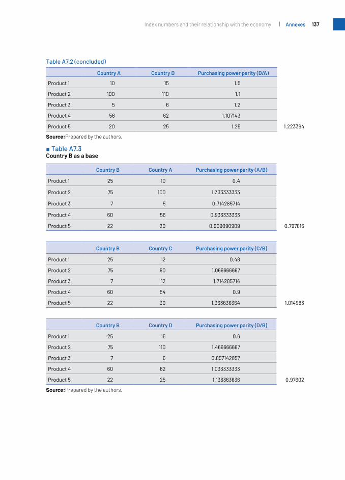
137Index numbers and their relationship with the economy Annexes
Country A Country D Purchasing power parity (D/A)
Product 1 10 15 1.5
Product 2 100 110 1.1
Product 3 5 6 1.2
Product 4 56 62 1.107143
Product 5 20 25 1.25 1.223364
Source: Prepared by the authors.
■ Table A7.3 Country B as a base
Country B Country A Purchasing power parity (A/B)
Product 1 25 10 0.4
Product 2 75 100 1.333333333
Product 3 7 5 0.714285714
Product 4 60 56 0.933333333
Product 5 22 20 0.909090909 0.797816
Country B Country C Purchasing power parity (C/B)
Product 1 25 12 0.48
Product 2 75 80 1.066666667
Product 3 7 12 1.714285714
Product 4 60 54 0.9
Product 5 22 30 1.363636364 1.014983
Country B Country D Purchasing power parity (D/B)
Product 1 25 15 0.6
Product 2 75 110 1.466666667
Product 3 7 6 0.857142857
Product 4 60 62 1.033333333
Product 5 22 25 1.136363636 0.97602
Source: Prepared by the authors.
Table A7.2 (concluded)

138 Economic Commission for Latin America and the Caribbean (ECLAC)Annexes
■ Table A7.4 Country C as a base
Country C Country A Purchasing power parity (A/C)
Product 1 12 10 0.833333
Product 2 80 100 1.25
Product 3 12 5 0.416667
Product 4 54 56 1.037037
Product 5 30 20 0.666667 0.786039
Country C Country B Purchasing power parity (B/C)
Product 1 12 25 2.083333
Product 2 80 75 0.9375
Product 3 12 7 0.583333
Product 4 54 60 1.111111
Product 5 30 22 0.733333 0.985238
Country C Country D Purchasing power parity (D/C)
Product 1 12 15 1.25
Product 2 80 110 1.375
Product 3 12 6 0.5
Product 4 54 62 1.148148
Product 5 30 25 0.833333 0.961612
Source: Prepared by the authors.
■ Table A7.5 Country D as a base
Country D Country A Purchasing Power Parity (P/P)
Product 1 15 10 0.666667
Product 2 110 100 0.909091
Product 3 6 5 0.833333
Product 4 62 56 0.903226
Product 5 25 20 0.8 0.817418

139Index numbers and their relationship with the economy Annexes
Country D Country B Purchasing power parity (B/D)
Product 1 15 25 1.666667
Product 2 110 75 0.681818
Product 3 6 7 1.166667
Product 4 62 60 0.967742
Product 5 25 22 0.88 1.024569
Country D Country C Purchasing power parity (C/D)
Product 1 15 12 0.8
Product 2 110 80 0.727273
Product 3 6 12 2
Product 4 62 54 0.870968
Product 5 25 30 1.2 1.03992
Source: Prepared by the authors.
■ Table A7.6 Summary of the purchasing power parity of a basic heading
A B C D
Base A 1.0000 1.2534 1.2722 1.2234
Base B 0.7978 1.0000 1.0150 0.9760
Base C 0.7860 0.9852 1.0000 0.9616
Base D 0.8174 1.0246 1.0399 1.0000
Source: Prepared by the authors.
(ii) Check the transitivity of the parities obtained.
■ Table A7.7 Transitivity
Parity B/A 1.253
Parity B/C * C/A 1.253
Parity B/D * D/A 1.253
Source: Prepared by the authors.
(iii) Based on the matrix in table A7.8, calculate the PPP of the basic heading in the case of an incomplete matrix, using the Jevons-GEKS (Gini-Eltetö-Köves-Szulc) method.PerformthecalculationbyfirsttakingcountryAasthebasecountry,then country B and so on.
Table A7.5 (concluded)

140 Economic Commission for Latin America and the Caribbean (ECLAC)Annexes
■ Table A7.8 Price matrix
Country A Country B Country C Country D
Product 1 10 12 15
Product 2 100 75 110
Product 3 7 12
Product 4 56 60 54
Product 5 22 30 25
Quantity of products j by country (Nj) 3 4 4 3
Source: Prepared by the authors.
Answer
■ Table A7.9 Country A as base
Country A Country B Purchasing power parity (B/A)
Product 1 10
Product 2 100 75 0.75
Product 3 7
Product 4 56 60 1.071428571
Product 5 22 0.896421
Country A Country C Purchasing power parity (C/A)
Product 1 10 12 1.2
Product 2 100
Product 3 12
Product 4 56 54 0.964285714
Product 5 30 1.075706
Country A Country D Purchasing power parity (D/A)
Product 1 10 15 1.5
Product 2 100 110 1.1
Product 3
Product 4 56
Product 5 25 1.284523
Source: Prepared by the authors.

141Index numbers and their relationship with the economy Annexes
■ Table A7.10 Country B as base
Country B Country A Purchasing power parity (A/B)
Product 1 10
Product 2 75 100 1.333333
Product 3 7
Product 4 60 56 0.933333
Product 5 22 1.115547
Country B Country C Purchasing power parity (C/B)
Product 1 12
Product 2 75
Product 3 7 12 1.714286
Product 4 60 54 0.9
Product 5 22 30 1.363636 1.281371
Country B Country D Purchasing power parity (D/B)
Product 1 15
Product 2 75 110 1.466667
Product 3 7
Product 4 60
Product 5 22 25 1.136364 1.290994
Source: Prepared by the authors.
■ Table A7.11 Country C as base
Country C Country A Purchasing power parity (A/C)
Product 1 12 10 0.833333
Product 2 100
Product 3 12
Product 4 54 56 1.037037
Product 5 30 0.929622

142 Economic Commission for Latin America and the Caribbean (ECLAC)Annexes
Table A7.11 (concluded)
Country C Country B Purchasing power parity (B/C)
Product 1 12
Product 2 75
Product 3 12 7 0.583333
Product 4 54 60 1.111111
Product 5 30 22 0.733333 0.780414
Country C Country D Purchasing power parity (D/C)
Product 1 12 15 1.25
Product 2 110
Product 3 12
Product 4 54
Product 5 30 25 0.833333 1.020621
Source: Prepared by the authors.
■ Table A7.12 Country D as a base
Country D Country A Purchasing power parity (A/D)
Product 1 15 10 0.666667
Product 2 110 100 0.909091
Product 3
Product 4 56
Product 5 25 0.778499
Country D Country B Purchasing power parity (B/D)
Producto 1 15
Producto 2 110 75 0.681818
Producto 3 7
Producto 4 60
Producto 5 25 22 0.88 0.774597

143Index numbers and their relationship with the economy Annexes
Country D Country C Purchasing power parity (C/D)
Producto 1 15 12 0.8
Producto 2 110
Producto 3 12
Producto 4 54
Producto 5 25 30 1.2 0.979796
Source: Prepared by the authors.
■ Table A7.13 Summary of the non-transitive purchasing power parity of a basic heading
A B C D
Base A 1.0000 0.8964 1.0757 1.2845
Base B 1.1155 1.0000 1.2814 1.2910
Base C 0.9296 0.7804 1.0000 1.0206
Base D 0.7785 0.7746 0.9798 1.0000
Source: Prepared by the authors.
(iv) Check transitivity before applying the Jevons-GEKS method.
■ Table A7.14 Non-transitive
Parity B/A 0.896
Parity B/C * C/A 0.839
Parity B/D * D/A 0.995
Source: Prepared by the authors.
(v) Check transitivity after applying the Jevons-GEKS method.
■ Table A7.15 Purchasing power parity. Jevons-GEKS
A B C D
Base A 1.0000 0.9051 1.1373 1.2033
Base B 1.1048 1.0000 1.2565 1.0581
Base C 0.8793 0.7959 1.0000 1.0581
Base D 0.9869 0.7522 0.9451 1.0000
Transitive
Parity B/A 0.905
Parity B/C * C/A 0.905
Parity B/D * D/A 0.905
Source: Prepared by the authors.
Table A7.12 (concluded)
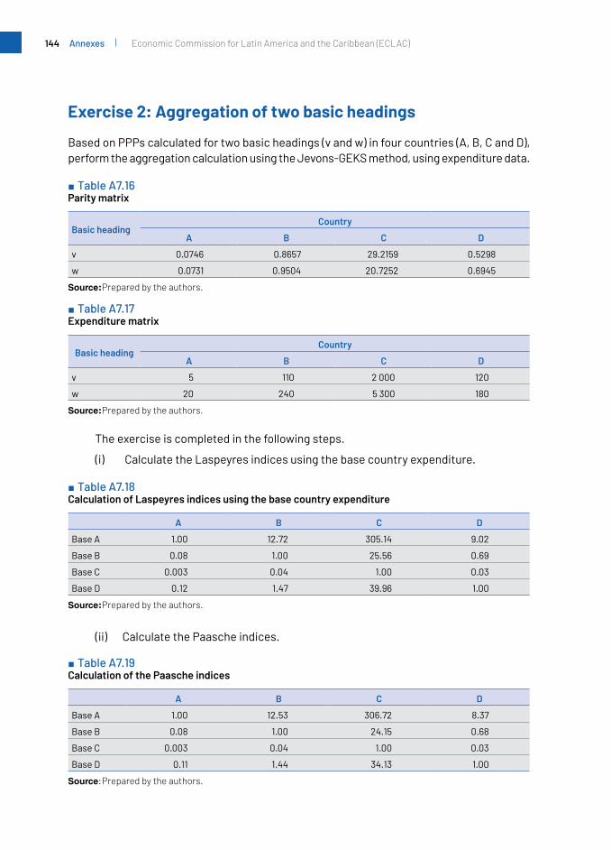
144 Economic Commission for Latin America and the Caribbean (ECLAC)Annexes
Exercise 2: Aggregation of two basic headings
Based on PPPs calculated for two basic headings (v and w) in four countries (A, B, C and D), perform the aggregation calculation using the Jevons-GEKS method, using expenditure data.
■ Table A7.16 Parity matrix
Basic headingCountry
A B C D
v 0.0746 0.8657 29.2159 0.5298
w 0.0731 0.9504 20.7252 0.6945
Source: Prepared by the authors.
■ Table A7.17 Expenditure matrix
Basic headingCountry
A B C D
v 5 110 2 000 120
w 20 240 5 300 180
Source: Prepared by the authors.
The exercise is completed in the following steps.
(i) Calculate the Laspeyres indices using the base country expenditure.
■ Table A7.18 Calculation of Laspeyres indices using the base country expenditure
A B C D
Base A 1.00 12.72 305.14 9.02
Base B 0.08 1.00 25.56 0.69
Base C 0.003 0.04 1.00 0.03
Base D 0.12 1.47 39.96 1.00
Source: Prepared by the authors.
(ii) Calculate the Paasche indices.
■ Table A7.19 Calculation of the Paasche indices
A B C D
Base A 1.00 12.53 306.72 8.37
Base B 0.08 1.00 24.15 0.68
Base C 0.003 0.04 1.00 0.03
Base D 0.11 1.44 34.13 1.00
Source: Prepared by the authors.

145Index numbers and their relationship with the economy Annexes
(iii) Calculate the Fisher indices.
■ Table A7.20 Calculation of Fisher indices
A B C D
Base A 1.0000 12.6244 305.9281 8.6893
Base B 0.0792 1.0000 24.8438 0.6857
Base C 0.0033 0.0403 1.0000 0.0271
Base D 0.1151 1.4583 36.9331 1.0000
Source: Prepared by the authors.
(iv) Apply the Jevons-GEKS method.
■ Table A7.21 Application of the Jevons-GEKS method
A B C D
Base A 1.0000 12.5578 311.5419 8.5779
Base B 0.0796 1.0000 24.8086 0.6831
Base C 0.0032 0.0403 1.0000 0.0275
Base D 0.1166 1.4640 36.3190 1.0000
Source: Prepared by the authors.
(v) Check transitivity.
■ Table A7.22 Transitivity
EKSa A/C = 0.0032
EKS A/B / EKS C/B 0.0032
EKS A/D / EKS C/D 0.0032
Source: Prepared by the authors.a EKS: Eltetö-Köves-Szulc.
Multiplying, by EKS A/B, all the elements in the row that takes country A as the base, gives the row that takes country B as base.
■ Table A7.23 Change of base
A B C D
Base A 1.0000 12.5578 311.5419 8.5779
EKSa A/B 0.0796 0.0796 0.0796 0.0796
Base B 0.0796 1.0000 24.8086 0.6831
Source: Prepared by the authors.a EKS: Eltetö-Köves-Szulc.

146 Economic Commission for Latin America and the Caribbean (ECLAC)Annexes
Annex A8
Quaranta tables, Dikhanov tables and benchmark parities
1. Quaranta tables
TheQuarantatableiscomposedoffoursubtables.Thefirstshowsthenameofthebasicheading, the code, the date on which the table was prepared, the period to which it refers, the method used to calculate the average prices of each of the products making up the basic heading, and the method used to calculate the basic heading parities.
The second subtable presents the information in summary form, for example the number of products included in the basic heading analysis, the number of countries that priced products, the country being used as a base for calculating the PPP, the average weightofthebasicheadinginthenationalaccountsandtheaveragecoefficientofvariation.The latter takes into account the variability of all basic heading products in all countries.
A Quaranta table is produced for each basic heading included in the product list. Its format is shown in table A8.1, using rice as an example.
■ Table A8.1 Quaranta table
DIAGNOSTIC ANALYSIS BY QUARANTUM TABLE - Rice
Data selection criteria
Basic heading code 99.11.01.11.1 Period of time AnnualDate of production of table
4/13/2011
Method of obtaining the average
Arithmetic mean Imputation CPD
Summary Information
Number of products included in the analysis 6 of 6 Average weight of the basic
heading in total expenditure 0.0
Number of countries included in the analysis 18 of 18 Averagecoefficientofvariation 27.4
Base country United States
Country level details
# The weights are multiplied by 10 000
Countries XR PPP PLI (%) Weight# Items Coeff. var.
Country 1 4.42 1.815 48.08 0 2;*0 7.2
Country 2 959.04 718.277 74.90 0 5;*0 8.2
Country 3 1 018.4 2.7696 0.27 0 2;*0 33.8

147Index numbers and their relationship with the economy Annexes
Details at the product level
99.11.01.11.1.01 Long grain rice, pre-packaged Coeff. var. 25.9 1-kg
Countries NC-price Price quotes
Coeff. var. XR-price XR-ratio CUP-price CUP-ratio Pref. UoM
Country 1 1,500 151 11.2 0.34 45.89 0.83 95.02 n.a.
Country 2 - - - - - - - n.a.
Country 3 766,381 10 3 72.93 9 857.6 1.14 130.66 n.a.
Source: Prepared by the authors. Note: CPD: country-product-dummy method In the details at the country level, XR: market exchange rate
between the national currency and that of the base country; PPP: purchasing power parity; PLI: price level index (PPP/XR); Weight: weighting of the basic heading provided by the national accounts offices; Items: the first number indicates the quantity of products quoted and the second the quantity of products that are important; Coeff. var.: coefficient of variation within each country for all products that make up the basic heading. In the details at the product level, NC-price: average price of the product expressed in national currency; Price quotes: number of observations; Coeff. var coefficient of variation of product observations in each country; XR-price: average domestic price converted into the base country’s currency, using the market exchange rate; XR-ratio: XR-price/average XR-price; CUP-price: national average price of each country converted into the base country currency, using PPPs; CUP-ratio: PPP price/average PPP price; Pref. UoM: preferred unit of measure; n.a.: not available.
The indicators in Subtable 3 (country level details) are explained below:
• XR: market exchange rate between the national and base country currency.
• PPP: purchasing power parity. This is calculated for the basic heading from the average prices, using the CPD method. It is expressed in units of the domestic currency per unit of the base country currency. It is a PPP-based exchange rate.
• PLI: Price level index (PPP/XR). A PLI higher than 100 means that the prices in the country concerned are higher than those in the base country.
• Weight: the weighting of the basic heading provided by the national accounts offices,multipliedby10,000. It isusedtogainanideaoftheimportanceofthebasic heading.
• Items:thefirstnumberindicatesthenumberofproductspricedandthesecondindicates the number of products that are important.
• Coeff.var.:thecoefficientofvariationwithineachcountryforallproductsthatmake up the basic heading.
The indicators included in subtable 4 (output level details) are explained below:
• NC-Price: average price of the product expressed in national currency.
• Price quotes: number of observations.
• Coeff.var.:coefficientofvariationofproductobservationsineachcountry
• XR-price: the national average price converted into the base country currency, using the market exchange rate. The geometric mean of all countries is shown.
• XR-ratio: (XR-price/average XR-price) gives a notion of the drift of the average price from the regional average, using the market exchange rate.
Table A8.1 (concluded)

148 Economic Commission for Latin America and the Caribbean (ECLAC)Annexes
• CUP-price: each country’s national average price converted into the base country currency, using PPPs. The geometric mean price is shown.
• CUP-ratio: (PPP-price/average PPP-price) gives an idea of the drift of the average price from the regional average, using PPPs.
• Pref UoM: is the preferred unit of measurement.
Productswithacoefficientofvariationabove33%,orwheretheratioswereoutsidethe range (80%–125%), were taken as critical values for review. The validation ranges proposed in the ICP KIT programme were also used, highlighting the magnitude of the deviations from the average prices with different colours.
2. Dikhanov tablesThe Dikhanov table consists of two subtables, the format of which is shown in table A8.2.
■ Table A8.2 Dikhanov table
Dikhanov temporal analysis Country 1 Country 2 Country 3
Period Annual–2005 Annual–2005 Annual–2005
PPP 2.934690064 658.1289976 4.040426119
STD 0.245237431 0.256006128 0.291549487
No. of priced items 420 513 572
ER (LCU/US$) 2.43 527.47 5.78
Rebased_XR 4.418181818 959.0363636 10.50909091
PLI 0.664230261 0.686239878 0.384469613
Details at the aggregate or basic heading level Country 1 Country 2 Country 3
Item code Item name Annual–2005 Annual–2005 Annual–2005
99.11.01.11.1 Rice
PPP 1.81507 718.297 4.84856
STD 0.05109 0.0726994 0.274263
PLI 0.410819 0.748978 0.461368
No. of priced items 2 5 6
99.11.01.11.1.01 Long grain rice. pre-packaged -0.5109 - 0.26746
Average price 1.5 - 5.51
No. of observations 151 - 10
Coefficientofvariation 11.2214 - 3
XR ratio 70.4386 - 108.78
Source: Prepared by the authors, on the basis of a tool developed by Dikhanov and provided by the World Bank, with fictitious data.
Note: PPP: purchasing power parity; STD: standard deviation of the country-product-dummy (CPD) or country-product-representative-dummy (CPRD) method; No. of priced items: quantity of products specified in the basic heading or in the aggregate; ER (LCU/US$): market exchange rate expressed as the number of local currency units per United States dollar; Rebased_XR: Exchange rates rebased in terms of the representative currency; PLI: price level index; Item code: code of the basic heading or aggregate; Item name: name of the basic heading or aggregate; Average price: average price in local currency; No. of observations: number of price observations; Coeff. var.: coefficient of variation of price observations; XR ratio: price ratios based on prices converted through the exchange rate.

149Index numbers and their relationship with the economy Annexes
Theindicatorsinthefirstsubtablearedetailedbelow:
• Period: period in which the prices of the products shown in the table were collected.
• PPP: Purchasing power parity for the basic heading or aggregate analysed in the table, expressed as the number of units of local currency per unit of the chosen base currency. The prices used to calculate the PPP are the average prices, expressed in local currency, provided by the countries on the products they priced for the basic heading or aggregate, in other words the average prices.
• STD: standard deviation of the residuals of the CPD or CPRD method of each country for the basic heading with the aggregate. This can be converted into a country’scoefficientofvariationbymultiplyingby100.
• No.ofpriceditems:quantityofproductsspecifiedinthebasicheadingorintheaggregate.
• ER (LCU/US$): Market exchange rate expressed as the number of local currency units per United States dollar.
• Rebased_XR: exchange rates rebased in terms of the base currency. Number of local currency units per unit of the base currency.
• PLI: Price level index. The PPPs expressed as the ratio of the corresponding exchange rates.
The second subtable contains the following information at the basic heading or aggregate level:
• Item code: code of the basic heading or aggregate shown in the table.
• Item name: name of the basic heading or aggregate shown in the table.
• PPP: PPP for the basic heading or aggregate analysed in the table, expressed as the number of units of local currency per units of the chosen base currency. The prices used to calculate the PPP are the average prices, expressed in local currency, provided by the countries on the products they priced for the basic heading or the aggregate, in other words the average prices.
• STD: standard deviation of the residuals of the CPD or CPRD method of each country for the basic heading with the aggregate. This can be converted into a country’scoefficientofvariationbymultiplyingby100.
• PLI: price level index. The PPPs expressed as the ratio of the corresponding exchange rates.
• No. of priced items: quantity of products specified in the basic heading or aggregate.
• Average price: average price in local currency.
• No. of observations: number of price observations on which the average price is based.
• Coefficientofvariation:Coefficientofvariationofthepriceobservations.
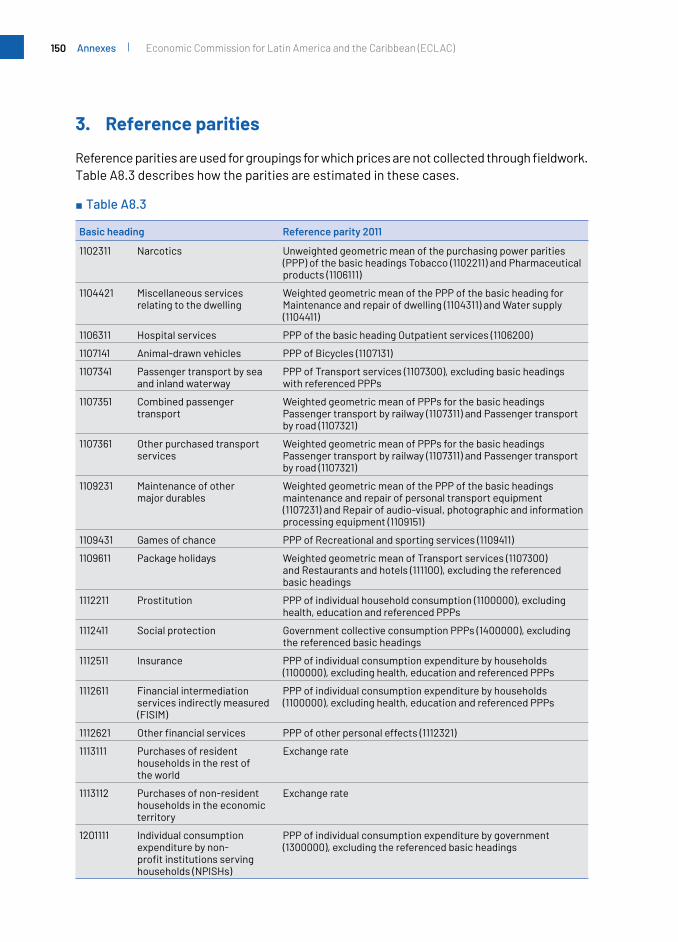
150 Economic Commission for Latin America and the Caribbean (ECLAC)Annexes
3. Reference parities
Referenceparitiesareusedforgroupingsforwhichpricesarenotcollectedthroughfieldwork.Table A8.3 describes how the parities are estimated in these cases.
■ Table A8.3
Basic heading Reference parity 2011
1102311 Narcotics Unweighted geometric mean of the purchasing power parities (PPP) of the basic headings Tobacco (1102211) and Pharmaceutical products (1106111)
1104421 Miscellaneous services relating to the dwelling
Weighted geometric mean of the PPP of the basic heading for Maintenance and repair of dwelling (1104311) and Water supply (1104411)
1106311 Hospital services PPP of the basic heading Outpatient services (1106200)
1107141 Animal-drawn vehicles PPP of Bicycles (1107131)
1107341 Passenger transport by sea and inland waterway
PPP of Transport services (1107300), excluding basic headings with referenced PPPs
1107351 Combined passenger transport
Weighted geometric mean of PPPs for the basic headings Passenger transport by railway (1107311) and Passenger transport by road (1107321)
1107361 Other purchased transport services
Weighted geometric mean of PPPs for the basic headings Passenger transport by railway (1107311) and Passenger transport by road (1107321)
1109231 Maintenance of other major durables
Weighted geometric mean of the PPP of the basic headings maintenance and repair of personal transport equipment (1107231) and Repair of audio-visual, photographic and information processing equipment (1109151)
1109431 Games of chance PPP of Recreational and sporting services (1109411)
1109611 Package holidays Weighted geometric mean of Transport services (1107300) and Restaurants and hotels (111100), excluding the referenced basic headings
1112211 Prostitution PPP of individual household consumption (1100000), excluding health, education and referenced PPPs
1112411 Social protection Government collective consumption PPPs (1400000), excluding the referenced basic headings
1112511 Insurance PPP of individual consumption expenditure by households (1100000), excluding health, education and referenced PPPs
1112611 Financial intermediation services indirectly measured (FISIM)
PPP of individual consumption expenditure by households (1100000), excluding health, education and referenced PPPs
1112621 Otherfinancialservices PPP of other personal effects (1112321)
1113111 Purchases of resident households in the rest of the world
Exchange rate
1113112 Purchases of non-resident households in the economic territory
Exchange rate
1201111 Individual consumption expenditure by non-profitinstitutionsservinghouseholds (NPISHs)
PPP of individual consumption expenditure by government (1300000), excluding the referenced basic headings

151Index numbers and their relationship with the economy Annexes
Basic heading Reference parity 2011
1301111 Housing (government) PPP of current or imputed rent (1104111)
1302124 Hospital services (government)
PPP of government production of health services (1302200), excluding the referenced basic headings
1302221 Intermediate consumption (health services)
PPP of individual consumption expenditure by households (1100000), excluding health, education and referenced PPPs
1302231 Gross operating surplus (health services)
PPP of Gross capital formation (1500000), excluding the referenced basic headings
1302241 Net taxes on production (health services)
PPP of government production of health services (1302200), excluding the referenced basic headings
1302251 Receipts from sales (health) PPP of government production of health services (1302200), excluding the referenced basic headings
1303111 Recreation and culture (government)
Weighted geometric mean of PPPs of Recreational and sporting services (1109411) and Cultural services (1109421)
1304111 Educationbenefitsandreimbursements
PPP of Government production of education services (1304200), excluding the referenced basic headings
1304221 Intermediate consumption (education)
PPP of Individual consumption by households (1100000), excluding health, education and reference PPPs
1304231 Gross operating surplus (education)
PPP of Gross capital formation (1500000), excluding the referenced basic headings
1304241 Net taxes on production (education)
PPP of Government production of education services (1304200), excluding the referenced basic headings
1304251 Receipts from sales (education)
PPP of Government production of education services (1304200), excluding the referenced basic headings
1305111 Social protection (government)
PPP of Collective consumption expenditure by government (1400000), excluding the referenced basic heading
1401121 Intermediate consumption (collective services)
PPP of Individual consumption by households (1100000), excluding health, education and referenced PPPs
1401131 Gross operating surplus (collective services)
PPP of Gross capital formation (1500000), excluding the referenced basic headings
1401141 Net taxes on production (collective services)
PPP of Collective consumption expenditure by government (1400000), excluding the referenced basic headings
1401151 Receipts from sales (collective services)
PPP of Collective consumption expenditure by government (1400000), excluding the referenced basic headings
1501212 Other road transport PPP of Motor vehicles, trailers and semi-trailers (1501211)
1501221 Other transport equipment PPP of Machinery and equipment (1501000), excluding the referenced basic headings
1503111 Other products PPP of Gross capital formation (1500000), excluding the referenced basic headings
1601111 Opening value of inventories PPP of goods
1601112 Closing value of inventories PPP of goods
1602111 Acquisitions of valuables Exchange rate
1602112 Disposals of valuables Exchange rate
1701111 Exports of goods and services Exchange rate
1701112 Imports of goods and services Exchange rate
Source: Prepared by the authors, on the basis of World Bank, ICP Classification [online] pubdocs.worldbank.org/en/.../06-26-2017-ICP-Classification.xlsx.
Table A8.3 (concluded)

Inde
x nu
mbe
rs a
nd th
eir r
elat
ions
hip
wit
h th
e ec
onom
yN
o. 1
Index numbers are the basic tool for synthesizing economic statistics, to
enable the formulae used to express and describe variables such as a
country’s economic growth or an economy’s inflation rate, and also to make
international comparisons. If different formulae are used, the results vary,
and comparisons are not valid; so it is important to understand the formulae
being used. Moreover, countries and international organizations need to
promote common practices that harmonize and standardize measurements.
Although index numbers are associated with macroeconomics, their theoretical
foundation lies in microeconomics.
This publication summarizes the links between price and volume indices and
microeconomic theory; and it presents the formulae that are recommended for
international measurements, and explains how to use them in international
price and volume comparisons.
The ECLAC Methodologies collection disseminates the conceptual bases,
technical specifications and applications of the quantitative and qualitative
instruments produced and used by ECLAC as part of its work. The ultimate
aim of the collection is to contribute more and better tools for evidence-
based policymaking to foster sustainable development with equality.


![Bernoulli Numbers and Various Consequences[3] In order to actually find out how the Bernoulli numbers behave, we can actually use a relationship between the Bernoulli numbers and the](https://static.fdocuments.us/doc/165x107/5e2b805e125b4477d37689bf/bernoulli-numbers-and-various-consequences-3-in-order-to-actually-find-out-how.jpg)