PDF generated using the open source mwlib toolkit. See http://code.pediapress.com/ for more information.PDF generated at: Mon, 25 Oct 2010 08:51:59 UTC

Neuro Fuzzy

ContentsArticles

Artificial neural network 1Supervised learning 12Semi-supervised learning 18Active learning (machine learning) 19Structured prediction 20Learning to rank 21Unsupervised learning 27Reinforcement learning 28Fuzzy logic 37Fuzzy set 44Fuzzy number 46

ReferencesArticle Sources and Contributors 47Image Sources, Licenses and Contributors 48

Article LicensesLicense 49

Artificial neural network 1

Artificial neural networkAn artificial neural network (ANN), usually called "neural network" (NN), is a mathematical model orcomputational model that is inspired by the structure and/or functional aspects of biological neural networks. Itconsists of an interconnected group of artificial neurons and processes information using a connectionist approach tocomputation. In most cases an ANN is an adaptive system that changes its structure based on external or internalinformation that flows through the network during the learning phase. Modern neural networks are non-linearstatistical data modeling tools. They are usually used to model complex relationships between inputs and outputs orto find patterns in data.

An artificial neural network is an interconnected group of nodes, akin to the vast networkof neurons in the human brain.

Background

The original inspiration for the termArtificial Neural Network came fromexamination of central nervoussystems and their neurons, axons,dendrites and synapses whichconstitute the processing elements ofbiological neural networks investigatedby neuroscience. In an artificial neuralnetwork simple artificial nodes, calledvariously "neurons", "neurodes","processing elements" (PEs) or "units",are connected together to form anetwork of nodes mimicking thebiological neural networks — hencethe term "artificial neural network".

Because neuroscience is still full ofquestions and because there are manylevels of abstraction and many ways totake inspiration from the brain, there isno single formal definition of what an artificial neural network is. Most would agree that it involves a network ofsimple processing elements which can exhibit complex global behavior determined by the connections between theprocessing elements and element parameters. While an artificial neural network does not have to be adaptive per se,its practical use comes with algorithms designed to alter the strength (weights) of the connections in the network toproduce a desired signal flow.These networks are also similar to the biological neural networks in the sense that functions are performedcollectively and in parallel by the units, rather than there being a clear delineation of subtasks to which various unitsare assigned (see also connectionism). Currently, the term Artificial Neural Network (ANN) tends to refer mostly toneural network models employed in statistics, cognitive psychology and artificial intelligence. Neural networkmodels designed with emulation of the central nervous system (CNS) in mind are a subject of theoreticalneuroscience and computational neuroscience.In modern software implementations of artificial neural networks, the approach inspired by biology has for the most part been abandoned for a more practical approach based on statistics and signal processing. In some of these systems, neural networks or parts of neural networks (such as artificial neurons) are used as components in larger systems that combine both adaptive and non-adaptive elements. While the more general approach of such adaptive

Artificial neural network 2

systems is more suitable for real-world problem solving, it has far less to do with the traditional artificial intelligenceconnectionist models. What they do have in common, however, is the principle of non-linear, distributed, paralleland local processing and adaptation.

ModelsNeural network models in artificial intelligence are usually referred to as artificial neural networks (ANNs); these areessentially simple mathematical models defining a function or a distribution over or both and , butsometimes models also intimately associated with a particular learning algorithm or learning rule. A common use ofthe phrase ANN model really means the definition of a class of such functions (where members of the class areobtained by varying parameters, connection weights, or specifics of the architecture such as the number of neuronsor their connectivity).

Network function

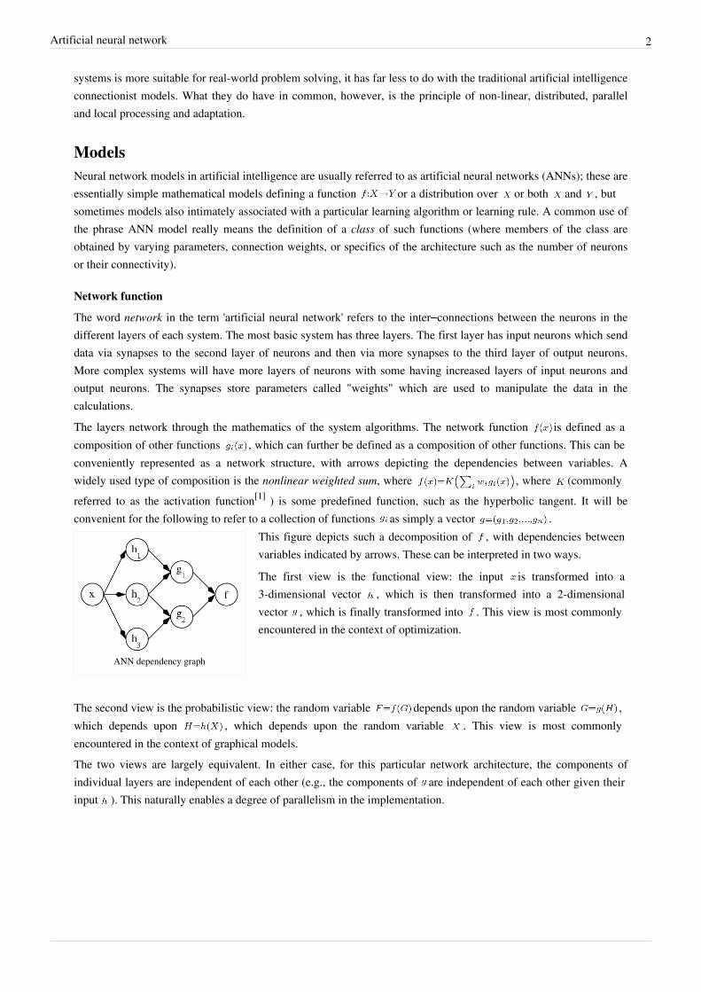
The word network in the term 'artificial neural network' refers to the inter–connections between the neurons in thedifferent layers of each system. The most basic system has three layers. The first layer has input neurons which senddata via synapses to the second layer of neurons and then via more synapses to the third layer of output neurons.More complex systems will have more layers of neurons with some having increased layers of input neurons andoutput neurons. The synapses store parameters called "weights" which are used to manipulate the data in thecalculations.The layers network through the mathematics of the system algorithms. The network function is defined as acomposition of other functions , which can further be defined as a composition of other functions. This can beconveniently represented as a network structure, with arrows depicting the dependencies between variables. Awidely used type of composition is the nonlinear weighted sum, where , where (commonlyreferred to as the activation function[1] ) is some predefined function, such as the hyperbolic tangent. It will beconvenient for the following to refer to a collection of functions as simply a vector .

ANN dependency graph

This figure depicts such a decomposition of , with dependencies betweenvariables indicated by arrows. These can be interpreted in two ways.

The first view is the functional view: the input is transformed into a3-dimensional vector , which is then transformed into a 2-dimensionalvector , which is finally transformed into . This view is most commonlyencountered in the context of optimization.

The second view is the probabilistic view: the random variable depends upon the random variable ,which depends upon , which depends upon the random variable . This view is most commonlyencountered in the context of graphical models.The two views are largely equivalent. In either case, for this particular network architecture, the components ofindividual layers are independent of each other (e.g., the components of are independent of each other given theirinput ). This naturally enables a degree of parallelism in the implementation.

Artificial neural network 3

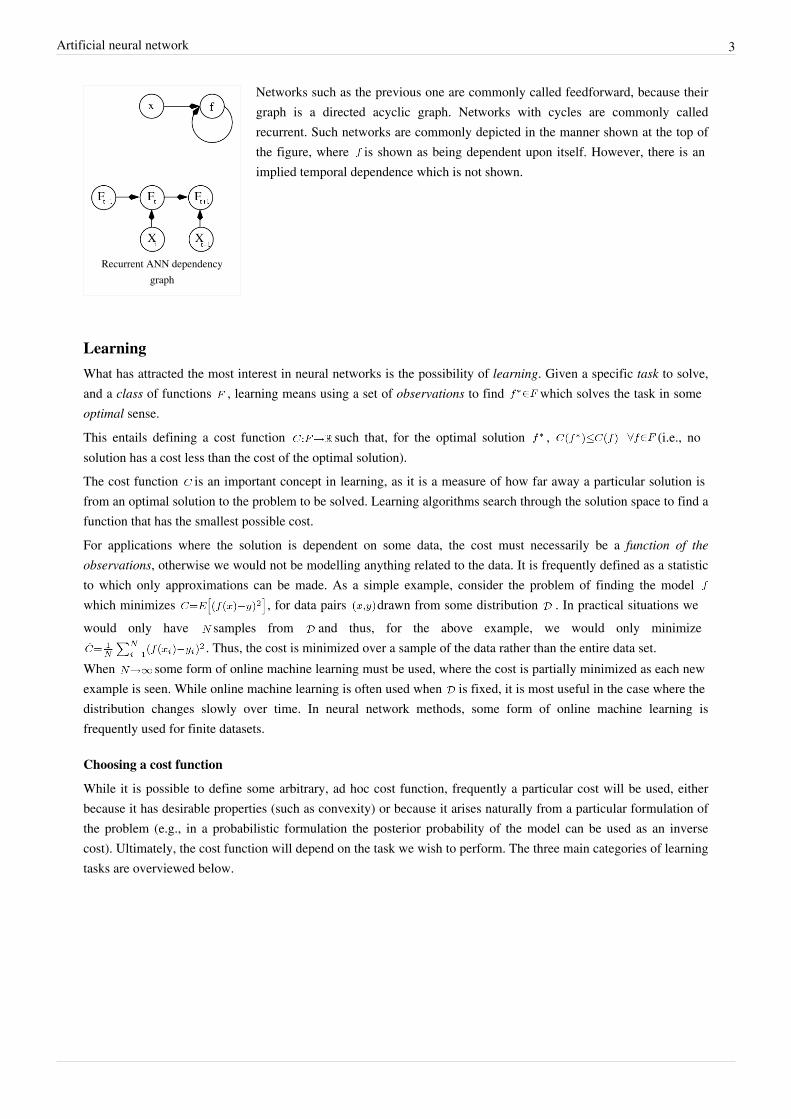
Recurrent ANN dependencygraph

Networks such as the previous one are commonly called feedforward, because theirgraph is a directed acyclic graph. Networks with cycles are commonly calledrecurrent. Such networks are commonly depicted in the manner shown at the top ofthe figure, where is shown as being dependent upon itself. However, there is animplied temporal dependence which is not shown.

LearningWhat has attracted the most interest in neural networks is the possibility of learning. Given a specific task to solve,and a class of functions , learning means using a set of observations to find which solves the task in someoptimal sense.This entails defining a cost function such that, for the optimal solution , (i.e., nosolution has a cost less than the cost of the optimal solution).The cost function is an important concept in learning, as it is a measure of how far away a particular solution isfrom an optimal solution to the problem to be solved. Learning algorithms search through the solution space to find afunction that has the smallest possible cost.For applications where the solution is dependent on some data, the cost must necessarily be a function of theobservations, otherwise we would not be modelling anything related to the data. It is frequently defined as a statisticto which only approximations can be made. As a simple example, consider the problem of finding the model which minimizes , for data pairs drawn from some distribution . In practical situations wewould only have samples from and thus, for the above example, we would only minimize

. Thus, the cost is minimized over a sample of the data rather than the entire data set.When some form of online machine learning must be used, where the cost is partially minimized as each newexample is seen. While online machine learning is often used when is fixed, it is most useful in the case where thedistribution changes slowly over time. In neural network methods, some form of online machine learning isfrequently used for finite datasets.

Choosing a cost function

While it is possible to define some arbitrary, ad hoc cost function, frequently a particular cost will be used, eitherbecause it has desirable properties (such as convexity) or because it arises naturally from a particular formulation ofthe problem (e.g., in a probabilistic formulation the posterior probability of the model can be used as an inversecost). Ultimately, the cost function will depend on the task we wish to perform. The three main categories of learningtasks are overviewed below.

Artificial neural network 4

Learning paradigmsThere are three major learning paradigms, each corresponding to a particular abstract learning task. These aresupervised learning, unsupervised learning and reinforcement learning. Usually any given type of networkarchitecture can be employed in any of those tasks.

Supervised learning

In supervised learning, we are given a set of example pairs and the aim is to find a function in the allowed class of functions that matches the examples. In other words, we wish to infer the mapping implied bythe data; the cost function is related to the mismatch between our mapping and the data and it implicitly containsprior knowledge about the problem domain.A commonly used cost is the mean-squared error which tries to minimize the average squared error between thenetwork's output, f(x), and the target value y over all the example pairs. When one tries to minimize this cost usinggradient descent for the class of neural networks called Multi-Layer Perceptrons, one obtains the common andwell-known backpropagation algorithm for training neural networks.Tasks that fall within the paradigm of supervised learning are pattern recognition (also known as classification) andregression (also known as function approximation). The supervised learning paradigm is also applicable to sequentialdata (e.g., for speech and gesture recognition). This can be thought of as learning with a "teacher," in the form of afunction that provides continuous feedback on the quality of solutions obtained thus far.

Unsupervised learning

In unsupervised learning we are given some data and the cost function to be minimized, that can be any functionof the data and the network's output, .The cost function is dependent on the task (what we are trying to model) and our a priori assumptions (the implicitproperties of our model, its parameters and the observed variables).As a trivial example, consider the model , where is a constant and the cost . Minimizingthis cost will give us a value of that is equal to the mean of the data. The cost function can be much morecomplicated. Its form depends on the application: for example, in compression it could be related to the mutualinformation between x and y, whereas in statistical modelling, it could be related to the posterior probability of themodel given the data. (Note that in both of those examples those quantities would be maximized rather thanminimized).Tasks that fall within the paradigm of unsupervised learning are in general estimation problems; the applicationsinclude clustering, the estimation of statistical distributions, compression and filtering.

Reinforcement learning

In reinforcement learning, data are usually not given, but generated by an agent's interactions with theenvironment. At each point in time , the agent performs an action and the environment generates an observation

and an instantaneous cost , according to some (usually unknown) dynamics. The aim is to discover a policy forselecting actions that minimizes some measure of a long-term cost; i.e., the expected cumulative cost. Theenvironment's dynamics and the long-term cost for each policy are usually unknown, but can be estimated.More formally, the environment is modeled as a Markov decision process (MDP) with states and actions

with the following probability distributions: the instantaneous cost distribution , the observationdistribution and the transition , while a policy is defined as conditional distribution overactions given the observations. Taken together, the two define a Markov chain (MC). The aim is to discover thepolicy that minimizes the cost; i.e., the MC for which the cost is minimal.ANNs are frequently used in reinforcement learning as part of the overall algorithm.

Artificial neural network 5

Tasks that fall within the paradigm of reinforcement learning are control problems, games and other sequentialdecision making tasks.See also: dynamic programming, stochastic control

Learning algorithmsTraining a neural network model essentially means selecting one model from the set of allowed models (or, in aBayesian framework, determining a distribution over the set of allowed models) that minimizes the cost criterion.There are numerous algorithms available for training neural network models; most of them can be viewed as astraightforward application of optimization theory and statistical estimation. Recent developments in this field useparticle swarm optimization and other swarm intelligence techniques.Most of the algorithms used in training artificial neural networks employ some form of gradient descent. This is doneby simply taking the derivative of the cost function with respect to the network parameters and then changing thoseparameters in a gradient-related direction.Evolutionary methods, simulated annealing, expectation-maximization and non-parametric methods are somecommonly used methods for training neural networks. See also machine learning.Temporal perceptual learning relies on finding temporal relationships in sensory signal streams. In an environment,statistically salient temporal correlations can be found by monitoring the arrival times of sensory signals. This isdone by the perceptual network.

Employing artificial neural networksPerhaps the greatest advantage of ANNs is their ability to be used as an arbitrary function approximation mechanismwhich 'learns' from observed data. However, using them is not so straightforward and a relatively goodunderstanding of the underlying theory is essential.• Choice of model: This will depend on the data representation and the application. Overly complex models tend to

lead to problems with learning.• Learning algorithm: There are numerous tradeoffs between learning algorithms. Almost any algorithm will work

well with the correct hyperparameters for training on a particular fixed dataset. However selecting and tuning analgorithm for training on unseen data requires a significant amount of experimentation.

• Robustness: If the model, cost function and learning algorithm are selected appropriately the resulting ANN canbe extremely robust.

With the correct implementation, ANNs can be used naturally in online learning and large dataset applications. Theirsimple implementation and the existence of mostly local dependencies exhibited in the structure allows for fast,parallel implementations in hardware.

ApplicationsThe utility of artificial neural network models lies in the fact that they can be used to infer a function fromobservations. This is particularly useful in applications where the complexity of the data or task makes the design ofsuch a function by hand impractical.

Real life applicationsThe tasks to which artificial neural networks are applied tend to fall within the following broad categories:• Function approximation, or regression analysis, including time series prediction, fitness approximation and

modeling.• Classification, including pattern and sequence recognition, novelty detection and sequential decision making.

Artificial neural network 6

• Data processing, including filtering, clustering, blind source separation and compression.• Robotics, including directing manipulators, Computer numerical control.Application areas include system identification and control (vehicle control, process control), quantum chemistry,[2]

game-playing and decision making (backgammon, chess, racing), pattern recognition (radar systems, faceidentification, object recognition and more), sequence recognition (gesture, speech, handwritten text recognition),medical diagnosis, financial applications (automated trading systems), data mining (or knowledge discovery indatabases, "KDD"), visualization and e-mail spam filtering.

Neural networks and neuroscienceTheoretical and computational neuroscience is the field concerned with the theoretical analysis and computationalmodeling of biological neural systems. Since neural systems are intimately related to cognitive processes andbehaviour, the field is closely related to cognitive and behavioural modeling.The aim of the field is to create models of biological neural systems in order to understand how biological systemswork. To gain this understanding, neuroscientists strive to make a link between observed biological processes (data),biologically plausible mechanisms for neural processing and learning (biological neural network models) and theory(statistical learning theory and information theory).

Types of models

Many models are used in the field defined at different levels of abstraction and modelling different aspects of neuralsystems. They range from models of the short-term behaviour of individual neurons, models of how the dynamics ofneural circuitry arise from interactions between individual neurons and finally to models of how behaviour can arisefrom abstract neural modules that represent complete subsystems. These include models of the long-term, andshort-term plasticity, of neural systems and their relations to learning and memory from the individual neuron to thesystem level.

Current research

While initially research had been concerned mostly with the electrical characteristics of neurons, a particularlyimportant part of the investigation in recent years has been the exploration of the role of neuromodulators such asdopamine, acetylcholine, and serotonin on behaviour and learning.Biophysical models, such as BCM theory, have been important in understanding mechanisms for synaptic plasticity,and have had applications in both computer science and neuroscience. Research is ongoing in understanding thecomputational algorithms used in the brain, with some recent biological evidence for radial basis networks andneural backpropagation as mechanisms for processing data.Computational devices have been created in CMOS for both biophysical simulation and neuromorphic computing.More recent efforts show promise for creating nanodevices for very large scale principal components analyses andconvolution. If successful, these effort could usher in a new era of neural computing that is a step beyond digitalcomputing, because it depends on learning rather than programming and because it is fundamentally analog ratherthan digital even though the first instantiations may in fact be with CMOS digital devices.

Artificial neural network 7

Neural network softwareNeural network software is used to simulate, research, develop and apply artificial neural networks, biologicalneural networks and in some cases a wider array of adaptive systems.

Types of artificial neural networksArtificial neural network types vary from those which have only one or two layers of single direction logic tocomplicated multi–input many directional feedback loop and layers. On the whole these sytems use algorithms intheir programming to determine control and organisation of their functions. Some may be as simple, one neuronlayer with an input and an output, and others can mimic complex systems such as dANN which can mimicchromosomal DNA through sizes at cellular level, into artificial organisms and simulate reproduction, mutation andpopulation sizes.[3]

Most sytems use "weights" to change the parameters of the throughput and the varying connections to the neurons.Artificial neural networks can be autonomous and learn by input from outside "teachers" or even self-teaching fromwritten in rules.

Theoretical properties

Computational powerThe multi-layer perceptron (MLP) is a universal function approximator, as proven by the Cybenko theorem.However, the proof is not constructive regarding the number of neurons required or the settings of the weights.Work by Hava Siegelmann and Eduardo D. Sontag has provided a proof that a specific recurrent architecture withrational valued weights (as opposed to full precision real number-valued weights) has the full power of a UniversalTuring Machine[4] using a finite number of neurons and standard linear connections. They have further shown thatthe use of irrational values for weights results in a machine with super-Turing power.

CapacityArtificial neural network models have a property called 'capacity', which roughly corresponds to their ability tomodel any given function. It is related to the amount of information that can be stored in the network and to thenotion of complexity.

ConvergenceNothing can be said in general about convergence since it depends on a number of factors. Firstly, there may existmany local minima. This depends on the cost function and the model. Secondly, the optimization method used mightnot be guaranteed to converge when far away from a local minimum. Thirdly, for a very large amount of data orparameters, some methods become impractical. In general, it has been found that theoretical guarantees regardingconvergence are an unreliable guide to practical application.

Generalisation and statisticsIn applications where the goal is to create a system that generalises well in unseen examples, the problem of overtraining has emerged. This arises in overcomplex or overspecified systems when the capacity of the network significantly exceeds the needed free parameters. There are two schools of thought for avoiding this problem: The first is to use cross-validation and similar techniques to check for the presence of overtraining and optimally select hyperparameters such as to minimize the generalisation error. The second is to use some form of regularisation. This is a concept that emerges naturally in a probabilistic (Bayesian) framework, where the regularisation can be performed by selecting a larger prior probability over simpler models; but also in statistical learning theory, where

Artificial neural network 8

the goal is to minimize over two quantities: the 'empirical risk' and the 'structural risk', which roughly corresponds tothe error over the training set and the predicted error in unseen data due to overfitting.

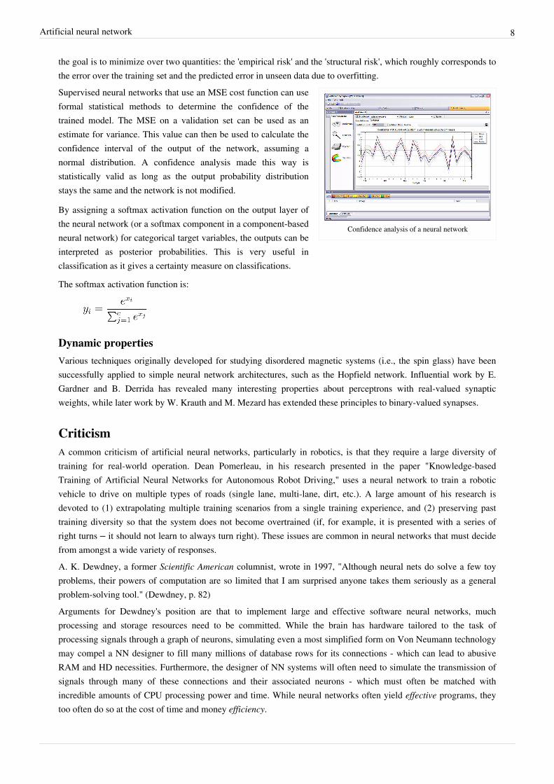
Confidence analysis of a neural network

Supervised neural networks that use an MSE cost function can useformal statistical methods to determine the confidence of thetrained model. The MSE on a validation set can be used as anestimate for variance. This value can then be used to calculate theconfidence interval of the output of the network, assuming anormal distribution. A confidence analysis made this way isstatistically valid as long as the output probability distributionstays the same and the network is not modified.

By assigning a softmax activation function on the output layer ofthe neural network (or a softmax component in a component-basedneural network) for categorical target variables, the outputs can beinterpreted as posterior probabilities. This is very useful inclassification as it gives a certainty measure on classifications.

The softmax activation function is:

Dynamic propertiesVarious techniques originally developed for studying disordered magnetic systems (i.e., the spin glass) have beensuccessfully applied to simple neural network architectures, such as the Hopfield network. Influential work by E.Gardner and B. Derrida has revealed many interesting properties about perceptrons with real-valued synapticweights, while later work by W. Krauth and M. Mezard has extended these principles to binary-valued synapses.

CriticismA common criticism of artificial neural networks, particularly in robotics, is that they require a large diversity oftraining for real-world operation. Dean Pomerleau, in his research presented in the paper "Knowledge-basedTraining of Artificial Neural Networks for Autonomous Robot Driving," uses a neural network to train a roboticvehicle to drive on multiple types of roads (single lane, multi-lane, dirt, etc.). A large amount of his research isdevoted to (1) extrapolating multiple training scenarios from a single training experience, and (2) preserving pasttraining diversity so that the system does not become overtrained (if, for example, it is presented with a series ofright turns – it should not learn to always turn right). These issues are common in neural networks that must decidefrom amongst a wide variety of responses.A. K. Dewdney, a former Scientific American columnist, wrote in 1997, "Although neural nets do solve a few toyproblems, their powers of computation are so limited that I am surprised anyone takes them seriously as a generalproblem-solving tool." (Dewdney, p. 82)Arguments for Dewdney's position are that to implement large and effective software neural networks, muchprocessing and storage resources need to be committed. While the brain has hardware tailored to the task ofprocessing signals through a graph of neurons, simulating even a most simplified form on Von Neumann technologymay compel a NN designer to fill many millions of database rows for its connections - which can lead to abusiveRAM and HD necessities. Furthermore, the designer of NN systems will often need to simulate the transmission ofsignals through many of these connections and their associated neurons - which must often be matched withincredible amounts of CPU processing power and time. While neural networks often yield effective programs, theytoo often do so at the cost of time and money efficiency.

Artificial neural network 9

Arguments against Dewdney's position are that neural nets have been successfully used to solve many complex anddiverse tasks, ranging from autonomously flying aircraft[5] to detecting credit card fraud.[6] Technology writer RogerBridgman commented on Dewdney's statements about neural nets:

Neural networks, for instance, are in the dock not only because they have been hyped to high heaven,(what hasn't?) but also because you could create a successful net without understanding how it worked:the bunch of numbers that captures its behaviour would in all probability be "an opaque, unreadabletable...valueless as a scientific resource". In spite of his emphatic declaration that science is nottechnology, Dewdney seems here to pillory neural nets as bad science when most of those devising themare just trying to be good engineers. An unreadable table that a useful machine could read would still bewell worth having.[7]

Some other criticisms came from believers of hybrid models (combining neural networks and symbolic approaches).They advocate the intermix of these two approaches and believe that hybrid models can better capture themechanisms of the human mind (Sun and Bookman 1994).

Gallery

A single-layer feedforwardartificial neural network. Arrowsoriginating from are omittedfor clarity. There are p inputs to

this network and q outputs. Thereis no activation function (orequivalently, the activation

function is ). In thissystem, the value of the qth

output, would be calculatedas

A two-layerfeedforward

artificial neuralnetwork.

See also• 20Q• Adaptive resonance theory• Artificial life• Associative memory• Autoencoder• Biological neural network• Biologically inspired computing• Blue brain• Cascade Correlation• Clinical decision support system• Connectionist expert system• Decision tree• Expert system

Artificial neural network 10

• Fuzzy logic• Genetic algorithm• In Situ Adaptive Tabulation• Linear discriminant analysis• Logistic regression• Memristor• Multilayer perceptron• Nearest neighbor (pattern recognition)• Neural network• Neuroevolution, NeuroEvolution of Augmented Topologies (NEAT)• Neural network software• Ni1000 chip• Optical neural network• Particle swarm optimization• Perceptron• Predictive analytics• Principal components analysis• Regression analysis• Simulated annealing• Systolic array• Time delay neural network (TDNN)

References[1] "The Machine Learning Dictionary" (http:/ / www. cse. unsw. edu. au/ ~billw/ mldict. html#activnfn). .[2] Roman M. Balabin, Ekaterina I. Lomakina (2009). "Neural network approach to quantum-chemistry data: Accurate prediction of density

functional theory energies". J. Chem. Phys. 131 (7): 074104. doi:10.1063/1.3206326. PMID 19708729.[3] "DANN:Genetic Wavelets" (http:/ / wiki. syncleus. com/ index. php/ DANN:Genetic_Wavelets). dANN project. . Retrieved 12 July 2010.[4] Siegelmann, H.T.; Sontag, E.D. (1991). "Turing computability with neural nets" (http:/ / www. math. rutgers. edu/ ~sontag/ FTP_DIR/

aml-turing. pdf). Appl. Math. Lett. 4 (6): 77–80. doi:10.1016/0893-9659(91)90080-F. .[5] "NASA NEURAL NETWORK PROJECT PASSES MILESTONE" (http:/ / www. nasa. gov/ centers/ dryden/ news/ NewsReleases/ 2003/

03-49. html). NASA. . Retrieved 12 July 2010.[6] "Counterfeit Fraud" (http:/ / www. visa. ca/ en/ personal/ pdfs/ counterfeit_fraud. pdf) (PDF). VISA. p. 1. . Retrieved 12 July 2010. "Neural

Networks (24/7 Monitoring):"[7] Roger Bridgman's defence of neural networks (http:/ / members. fortunecity. com/ templarseries/ popper. html)

Bibliography• Bar-Yam, Yaneer (2003). Dynamics of Complex Systems, Chapter 2 (http:/ / necsi. org/ publications/ dcs/

Bar-YamChap2. pdf).• Bar-Yam, Yaneer (2003). Dynamics of Complex Systems, Chapter 3 (http:/ / necsi. org/ publications/ dcs/

Bar-YamChap3. pdf).• Bar-Yam, Yaneer (2005). Making Things Work (http:/ / necsi. org/ publications/ mtw/ ). Please see Chapter 3• Bhadeshia H. K. D. H. (1999). " Neural Networks in Materials Science (http:/ / www. msm. cam. ac. uk/

phase-trans/ abstracts/ neural. review. pdf)". ISIJ International 39: 966–979. doi:10.2355/isijinternational.39.966.• Bhagat, P.M. (2005) Pattern Recognition in Industry, Elsevier. ISBN 0-08-044538-1• Bishop, C.M. (1995) Neural Networks for Pattern Recognition, Oxford: Oxford University Press. ISBN

0-19-853849-9 (hardback) or ISBN 0-19-853864-2 (paperback)• Cybenko, G.V. (1989). Approximation by Superpositions of a Sigmoidal function, Mathematics of Control,

Signals and Systems, Vol. 2 pp. 303–314. electronic version (http:/ / actcomm. dartmouth. edu/ gvc/ papers/

Artificial neural network 11

approx_by_superposition. pdf)• Duda, R.O., Hart, P.E., Stork, D.G. (2001) Pattern classification (2nd edition), Wiley, ISBN 0-471-05669-3• Egmont-Petersen, M., de Ridder, D., Handels, H. (2002). "Image processing with neural networks - a review".

Pattern Recognition 35 (10): 2279–2301. doi:10.1016/S0031-3203(01)00178-9.• Gurney, K. (1997) An Introduction to Neural Networks London: Routledge. ISBN 1-85728-673-1 (hardback) or

ISBN 1-85728-503-4 (paperback)• Haykin, S. (1999) Neural Networks: A Comprehensive Foundation, Prentice Hall, ISBN 0-13-273350-1• Fahlman, S, Lebiere, C (1991). The Cascade-Correlation Learning Architecture, created for National Science

Foundation, Contract Number EET-8716324, and Defense Advanced Research Projects Agency (DOD), ARPAOrder No. 4976 under Contract F33615-87-C-1499. electronic version (http:/ / www. cs. iastate. edu/ ~honavar/fahlman. pdf)

• Hertz, J., Palmer, R.G., Krogh. A.S. (1990) Introduction to the theory of neural computation, Perseus Books.ISBN 0-201-51560-1

• Lawrence, Jeanette (1994) Introduction to Neural Networks, California Scientific Software Press. ISBN1-883157-00-5

• Masters, Timothy (1994) Signal and Image Processing with Neural Networks, John Wiley & Sons, Inc. ISBN0-471-04963-8

• Ness, Erik. 2005. SPIDA-Web (http:/ / www. conbio. org/ cip/ article61WEB. cfm). Conservation in Practice6(1):35-36. On the use of artificial neural networks in species taxonomy.

• Ripley, Brian D. (1996) Pattern Recognition and Neural Networks, Cambridge• Siegelmann, H.T. and Sontag, E.D. (1994). Analog computation via neural networks, Theoretical Computer

Science, v. 131, no. 2, pp. 331–360. electronic version (http:/ / www. math. rutgers. edu/ ~sontag/ FTP_DIR/nets-real. pdf)

• Sergios Theodoridis, Konstantinos Koutroumbas (2009) "Pattern Recognition" , 4th Edition, Academic Press,ISBN 978-1-59749-272-0.

• Smith, Murray (1993) Neural Networks for Statistical Modeling, Van Nostrand Reinhold, ISBN 0-442-01310-8• Wasserman, Philip (1993) Advanced Methods in Neural Computing, Van Nostrand Reinhold, ISBN

0-442-00461-3

Further reading• Dedicated issue of Philosophical Transactions B on Neural Networks and Perception. Some articles are freely

available. (http:/ / publishing. royalsociety. org/ neural-networks)

External links• Performance comparison of neural network algorithms tested on UCI data sets (http:/ / tunedit. org/ results?e=&

d=UCI/ & a=neural+ rbf+ perceptron& n=)• A close view to Artificial Neural Networks Algorithms (http:/ / www. learnartificialneuralnetworks. com)• Neural Networks (http:/ / www. dmoz. org/ Computers/ Artificial_Intelligence/ Neural_Networks/ ) at the Open

Directory Project• A Brief Introduction to Neural Networks (D. Kriesel) (http:/ / www. dkriesel. com/ en/ science/ neural_networks)

- Illustrated, bilingual manuscript about artificial neural networks; Topics so far: Perceptrons, Backpropagation,Radial Basis Functions, Recurrent Neural Networks, Self Organizing Maps, Hopfield Networks.

• Neural Networks in Materials Science (http:/ / www. msm. cam. ac. uk/ phase-trans/ abstracts/ neural. review.html)

• A practical tutorial on Neural Networks (http:/ / www. ai-junkie. com/ ann/ evolved/ nnt1. html)

Artificial neural network 12

• Applications of neural networks (http:/ / www. peltarion. com/ doc/ index.php?title=Applications_of_adaptive_systems)

• Flood3 - Open source C++ library implementing the Multilayer Perceptron (http:/ / www. cimne. com/ flood/ )

Supervised learningSupervised learning is the machine learning task of inferring a function from supervised training data. The trainingdata consist of a set of training examples. In supervised learning, each example is a pair consisting of an input object(typically a vector) and a desired output value (also called the supervisory signal). A supervised learning algorithmanalyzes the training data and produces an inferred function, which is called a classifier (if the output is discrete, seeclassification) or a regression function (if the output is continuous, see regression). The inferred function shouldpredict the correct output value for any valid input object. This requires the learning algorithm to generalize from thetraining data to unseen situations in a "reasonable" way (see inductive bias). (Compare with unsupervised learning.)The parallel task in human and animal psychology is often referred to as concept learning.

OverviewIn order to solve a given problem of supervised learning, one has to perform various steps:1. Determine the type of training examples. Before doing anything else, the engineer should decide what kind of

data is to be used as an example. For instance, this might be a single handwritten character, an entire handwrittenword, or an entire line of handwriting.

2. Gather a training set. The training set needs to be representative of the real-world use of the function. Thus, a setof input objects is gathered and corresponding outputs are also gathered, either from human experts or frommeasurements.

3. Determine the input feature representation of the learned function. The accuracy of the learned function dependsstrongly on how the input object is represented. Typically, the input object is transformed into a feature vector,which contains a number of features that are descriptive of the object. The number of features should not be toolarge, because of the curse of dimensionality; but should contain enough information to accurately predict theoutput.

4. Determine the structure of the learned function and corresponding learning algorithm. For example, the engineermay choose to use support vector machines or decision trees.

5. Complete the design. Run the learning algorithm on the gathered training set. Some supervised learningalgorithms require the user to determine certain control parameters. These parameters may be adjusted byoptimizing performance on a subset (called a validation set) of the training set, or via cross-validation.

6. Evaluate the accuracy of the learned function. After parameter adjustment and learning, the performance of theresulting function should be measured on a test set that is separate from the training set.

A wide range of supervised learning algorithms is available, each with its strengths and weaknesses. There is nosingle learning algorithm that works best on all supervised learning problems (see the No free lunch theorem).There are four major issues to consider in supervised learning:

Bias-variance tradeoffA first issue is the tradeoff between bias and variance[1] . Imagine that we have available several different, but equally good, training data sets. A learning algorithm is biased for a particular input if, when trained on each of these data sets, it is systematically incorrect when predicting the correct output for . A learning algorithm has high variance for a particular input if it predicts different output values when trained on different training sets. The prediction error of a learned classifier is related to the sum of the bias and the variance of the learning algorithm[2] .

Supervised learning 13

Generally, there is a tradeoff between bias and variance. A learning algorithm with low bias must be "flexible" sothat it can fit the data well. But if the learning algorithm is too flexible, it will fit each training data set differently,and hence have high variance. A key aspect of many supervised learning methods is that they are able to adjust thistradeoff between bias and variance (either automatically or by providing a bias/variance parameter that the user canadjust).

Function complexity and amount of training dataThe second issue is the amount of training data available relative to the complexity of the "true" function (classifieror regression function). If the true function is simple, then an "inflexible" learning algorithm with high bias and lowvariance will be able to learn it from a small amount of data. But if the true function is highly complex (e.g., becauseit involves complex interactions among many different input features and behaves differently in different parts of theinput space), then the function will only be learnable from a very large amount of training data and using a "flexible"learning algorithm with low bias and high variance. Good learning algorithms therefore automatically adjust thebias/variance tradeoff based on the amount of data available and the apparent complexity of the function to belearned.

Dimensionality of the input spaceA third issue is the dimensionality of the input space. If the input feature vectors have very high dimension, thelearning problem can be difficult even if the true function only depends on a small number of those features. This isbecause the many "extra" dimensions can confuse the learning algorithm and cause it to have high variance. Hence,high input dimensionality typically requires tuning the classifier to have low variance and high bias. In practice, ifthe engineer can manually remove irrelevant features from the input data, this is likely to improve the accuracy ofthe learned function. In addition, there are many algorithms for feature selection that seek to identify the relevantfeatures and discard the irrelevant ones. This is an instance of the more general strategy of dimensionality reduction,which seeks to map the input data into a lower dimensional space prior to running the supervised learning algorithm.

Noise in the output valuesA fourth issue is the degree of noise in the desired output values (the supervisory targets). If the desired outputvalues are often incorrect (because of human error or sensor errors), then the learning algorithm should not attemptto find a function that exactly matches the training examples. This is another case where it is usually best to employa high bias, low variance classifier.

Other factors to considerOther factors to consider when choosing and applying a learning algorithm include the following:1. Heterogeneity of the data. If the feature vectors include features of many different kinds (discrete, discrete

ordered, counts, continuous values), some algorithms are easier to apply than others. Many algorithms, includingSupport Vector Machines, linear regression, logistic regression, neural networks, and nearest neighbor methods,require that the input features be numerical and scaled to similar ranges (e.g., to the [-1,1] interval). Methods thatemploy a distance function, such as nearest neighbor methods and support vector machines with Gaussiankernels, are particularly sensitive to this. An advantage of decision trees is that they easily handle heterogeneousdata.

2. Redundancy in the data. If the input features contain redundant information (e.g., highly correlated features),some learning algorithms (e.g., linear regression, logistic regression, and distance based methods) will performpoorly because of numerical instabilities. These problems can often by solved by imposing some form ofregularization.

Supervised learning 14

3. Presence of interactions and non-linearities. If each of the features makes an independent contribution to theoutput, then algorithms based on linear functions (e.g., linear regression, logistic regression, Support VectorMachines, naive Bayes) and distance functions (e.g., nearest neighbor methods, support vector machines withGaussian kernels) generally perform well. However, if there are complex interactions among features, thenalgorithms such as decision trees and neural networks work better, because they are specifically designed todiscover these interactions. Linear methods can also be applied, but the engineer must manually specify theinteractions when using them.

When considering a new application, the engineer can compare multiple learning algorithms and experimentallydetermine which one works best on the problem at hand (see cross validation. Tuning the performance of a learningalgorithm can be very time-consuming. Given fixed resources, it is often better to spend more time collectingadditional training data and more informative features than it is to spend extra time tuning the learning algorithms.The most widely used learning algorithms are Support Vector Machines, linear regression, logistic regression, naiveBayes, linear discriminant analysis, decision trees, k-nearest neighbor algorithm, and Neural Networks (Multilayerperceptron).

How supervised learning algorithms workGiven a set of training examples of the form , a learning algorithm seeks a function

, where is the input space and is the output space. The function is an element of some spaceof possible functions , usually called the hypothesis space. It is sometimes convenient to represent using ascoring function such that is defined as returning the value that gives the highest score:

. Let denote the space of scoring functions.Although and can be any space of functions, many learning algorithms are probabilistic models where takes the form of a conditional probability model , or takes the form of a joint probabilitymodel . For example, naive Bayes and linear discriminant analysis are joint probabilitymodels, whereas logistic regression is a conditional probability model.There are two basic approaches to choosing or : empirical risk minimization and structural risk minimization[3]

. Empirical risk minimization seeks the function that best fits the training data. Structural risk minimize includes apenalty function that controls the bias/variance tradeoff.In both cases, it is assumed that the training set consists of a sample of independent and identically distributed pairs,

. In order to measure how well a function fits the training data, a loss function isdefined. For training example , the loss of predicting the value is .The risk of function is defined as the expected loss of . This can be estimated from the training data as

.

Empirical risk minimization

In empirical risk minimization, the supervised learning algorithm seeks the function that minimizes .Hence, a supervised learning algorithm can be constructed by applying an optimization algorithm to find .When is a conditional probability distribution and the loss function is the negative log likelihood:

, then empirical risk minimization is equivalent to maximum likelihood estimation.When contains many candidate functions or the training set is not sufficiently large, empirical risk minimizationleads to high variance and poor generalization. The learning algorithm is able to memorize the training exampleswithout generalizing well. This is called overfitting.

Supervised learning 15

Structural risk minimizationStructural risk minimization seeks to prevent overfitting by incorporating a regularization penalty into theoptimization. The regularization penalty can be viewed as implementing a form of Occam's razor that prefers simplerfunctions over more complex ones.A wide variety of penalties have been employed that correspond to different definitions of complexity. For example,consider the case where the function is a linear function of the form

.

A popular regularization penalty is , which is the squared Euclidean norm of the weights, also known as the

norm. Other norms include the norm, , and the norm, which is the number of non-zero s.

The penalty will be denoted by .The supervised learning optimization problem is to find the function that minimizes

The parameter controls the bias-variance tradeoff. When , this gives empirical risk minimization with lowbias and high variance. When is large, the learning algorithm will have high bias and low variance. The value of

can be chosen empirically via cross validation.

The complexity penalty has a Bayesian interpretation as the negative log prior probability of , , inwhich case is the posterior probabability of .

Generative trainingThe training methods described above are discriminative training methods, because they seek to find a function that discriminates well between the different output values (see discriminative model). For the special case where

is a joint probability distribution and the loss function is the negative log likelihood

a risk minimization algorithm is said to perform generative training, because can be

regarded as a generative model that explains how the data were generated. Generative training algorithms are oftensimpler and more computationally efficient than discriminative training algorithms. In some cases, the solution canbe computed in closed form as in naive Bayes and linear discriminant analysis.

Generalizations of supervised learningThere are several ways in which the standard supervised learning problem can be generalized:1. Semi-supervised learning: In this setting, the desired output values are provided only for a subset of the training

data. The remaining data is unlabeled.2. Active learning: Instead of assuming that all of the training examples are given at the start, active learning

algorithms interactively collect new examples, typically by making queries to a human user. Often, the queries arebased on unlabeled data, which is a scenario that combines semi-supervised learning with active learning.

3. Structured prediction: When the desired output value is a complex object, such as a parse tree or a labeled graph,then standard methods must be extended.

4. Learning to rank: When the input is a set of objects and the desired output is a ranking of those objects, thenagain the standard methods must be extended.

Supervised learning 16

Approaches and algorithms• Analytical learning• Artificial neural network• Backpropagation• Boosting• Bayesian statistics• Case-based reasoning• Decision tree learning• Inductive logic programming• Gaussian process regression• Kernel estimators• Learning Automata• Minimum message length (decision trees, decision graphs, etc.)• Naive bayes classifier• Nearest Neighbor Algorithm• Probably approximately correct learning (PAC) learning• Ripple down rules, a knowledge acquisition methodology• Symbolic machine learning algorithms• Subsymbolic machine learning algorithms• Support vector machines• Random Forests• Ensembles of Classifiers• Ordinal Classification• Data Pre-processing• Handling imbalanced datasets• Statistical relational learning

Applications• Bioinformatics• Cheminformatics

• Quantitative structure-activity relationship• Database marketing• Handwriting recognition• Information retrieval

• Learning to rank• Object recognition in computer vision• Optical character recognition• Spam detection• Pattern recognition• Speech recognition• Forecasting Fraudulent Financial Statements

Supervised learning 17

General issues• Computational learning theory• Inductive bias• Overfitting (machine learning)• (Uncalibrated) Class membership probabilities• Version spaces

Notes[1] Geman et al., 1992[2] James, 2003[3] Vapnik, 2000

References• L. Breiman (1996). Heuristics of instability and stabilization in model selection. Annals of Statistics 24(6),

2350-2382.• G. James (2003) Variance and Bias for General Loss Functions, Machine Learning 51, 115-135. (http:/ /

www-bcf. usc. edu/ ~gareth/ research/ bv. pdf)• S. Geman, E. Bienenstock, and R. Doursat (1992). Neural networks and the bias/variance dilemma. Neural

Computation 4, 1–58.• Vapnik, V. N. The Nature of Statistical Learning Theory (2nd Ed.), Springer Verlag, 2000.

External links• Several supervised machine learning algorithm implementations in Ruby (http:/ / ai4r. rubyforge. org)

Semi-supervised learning 18

Semi-supervised learningIn computer science, semi-supervised learning is a class of machine learning techniques that make use of bothlabeled and unlabeled data for training - typically a small amount of labeled data with a large amount of unlabeleddata. Semi-supervised learning falls between unsupervised learning (without any labeled training data) andsupervised learning (with completely labeled training data). Many machine-learning researchers have found thatunlabeled data, when used in conjunction with a small amount of labeled data, can produce considerableimprovement in learning accuracy. The acquisition of labeled data for a learning problem often requires a skilledhuman agent to manually classify training examples. The cost associated with the labeling process thus may render afully labeled training set infeasible, whereas acquisition of unlabeled data is relatively inexpensive. In suchsituations, semi-supervised learning can be of great practical value.One example of a semi-supervised learning technique is co-training, in which two or possibly more learners are eachtrained on a set of examples, but with each learner using a different, and ideally independent, set of features for eachexample.An alternative approach is to model the joint probability distribution of the features and the labels. For the unlabelleddata the labels can then be treated as 'missing data'. Techniques that handle missing data, such as Gibbs sampling orthe EM algorithm, can then be used to estimate the parameters of the model.

See also• Constrained clustering• Transductive learning

References1. Abney, S., Semisupervised Learning for Computational Linguistics. Chapman & Hall/CRC, 2008.2. Blum, A., Mitchell, T. Combining labeled and unlabeled data with co-training [1]. COLT: Proceedings of the

Workshop on Computational Learning Theory, Morgan Kaufmann, 1998, p. 92-100.3. Chapelle, O., B. Schölkopf and A. Zien: Semi-Supervised Learning. MIT Press, Cambridge, MA (2006). Further

information [2].4. Huang T-M., Kecman V., Kopriva I. [3], "Kernel Based Algorithms for Mining Huge Data Sets, Supervised,

Semisupervised and Unsupervised Learning", Springer-Verlag, Berlin, Heidelberg, 260 pp. 96 illus., Hardcover,ISBN 3-540-31681-7, 2006.

5. O'Neill, T. J. (1978) Normal discrimination with unclassified observations. Journal of the American StatisticalAssociation, 73, 821–826.

6. Theodoridis S., Koutroumbas K. (2009) "Pattern Recognition" , 4th Edition, Academic Press, ISBN:978-1-59749-272-0.

7. Zhu, X. Semi-supervised learning literature survey [4].8. Zhu, X., Goldberg, A. Introduction to Semi-Supervised Learning [5]. Morgan & Claypool Publishers, 2009.

Semi-supervised learning 19

References[1] http:/ / www. cs. wustl. edu/ ~zy/ paper/ cotrain. ps[2] http:/ / www. kyb. tuebingen. mpg. de/ ssl-book/[3] http:/ / www. learning-from-data. com[4] http:/ / www. cs. wisc. edu/ ~jerryzhu/ pub/ ssl_survey. pdf[5] http:/ / www. morganclaypool. com/ doi/ abs/ 10. 2200/ S00196ED1V01Y200906AIM006

Active learning (machine learning)Active learning is a form of supervised machine learning in which the learning algorithm is able to interactivelyquery the user (or some other information source) to obtain the desired outputs at new data points. In statisticsliterature it is sometimes also called optimal experimental design.[1]

There are situations in which unlabeled data is abundant but labeling data is expensive. In such a scenario thelearning algorithm can actively query the user/teacher for labels. This type of iterative supervised learning is calledactive learning. Since the learner chooses the examples, the number of examples to learn a concept can often bemuch lower than the number required in normal supervised learning. With this approach there is a risk that thealgorithm might focus on unimportant or even invalid examples.Active learning can be especially useful in biological research problems such as Protein engineering where a fewproteins have been discovered with a certain interesting function and one wishes to determine which of manypossible mutants to make next that will have a similar function[2] .

DefinitionsLet be the total set of all data under consideration. For example, in a protein engineering problem, wouldinclude all proteins that are known to have a certain interesting activity and all additional proteins that one mightwant to test for that activity.During each iteration, , is broken up into three subsets

1. : Data points where the label is known.2. : Data points where the label is unknown.3. : A subset of that is chosen to be labeled.Most of the current research in active learning involves the best method to chose the data points for .

Minimum Marginal HyperplaneSome active learning algorithms are built upon Support vector machines (SVMs) and exploit the structure of theSVM to determine which data points to label. Such methods usually calculate the margin, , of each unlabeleddatum in and treat as an n-dimensional distance from that datum to separating hyperplane.Minimum Marginal Hyperplane methods assume that the data with the smallest are those that the SVM is mostuncertain about and therefore should be placed in to be labeled. Other similar methods, such as MaximumMarginal Hyperplane, choose data with the largest . Tradeoff methods choose a mix of the smallest and largest

s.

Active learning (machine learning) 20

Maximum CuriosityAnother active learning method, that typically learns a data set with fewer examples than Minimum MarginalHyperplane but is more computationally intensive and only works for discrete classifiers is Maximum Curiosity[3] .

Maximum curiosity takes each unlabeled datum in and assumes all possible labels that datum might have. Thisdatum with each assumed class is added to and then the new is cross-validated. It is assumed that whenthe datum is paired up with its correct label, the cross-validated accuracy (or correlation coefficient) of willmost improve. The datum with the most improved accuracy is placed in to be labeled

Notes[1] Settles, Burr (2009), "Active Learning Literature Survey" (http:/ / pages. cs. wisc. edu/ ~bsettles/ pub/ settles. activelearning. pdf), Computer

Sciences Technical Report 1648. University of Wisconsin–Madison, , retrieved 2010-09-14.[2] Danziger, S.A., Swamidass, S.J., Zeng, J., Dearth, L.R., Lu, Q., Chen, J.H., Cheng, J., Hoang, V.P., Saigo, H., Luo, R., Baldi, P., Brachmann,

R.K. and Lathrop, R.H. Functional census of mutation sequence spaces: the example of p53 cancer rescue mutants, (2006) IEEE/ACMtransactions on computational biology and bioinformatics, 3, 114-125.

[3] Danziger, S.A., Zeng, J., Wang, Y., Brachmann, R.K. and Lathrop, R.H. Choosing where to look next in a mutation sequence space:Active Learning of informative p53 cancer rescue mutants,(2007) Bioinformatics, 23(13), 104-114. (http:/ / bioinformatics. oxfordjournals.org/ cgi/ reprint/ 23/ 13/ i104. pdf)

Structured predictionStructured prediction is an umbrella term for machine learning and regression techniques that involve predictingstructured objects. For example, the problem of translating a natural language sentence into a semantic representationsuch as a parse tree can be seen as a structured prediction problem in which the structured output domain is the set ofall possible parse trees. Structured prediction generalizes supervised learning where the output domain is usually asmall or simple set.Probabilistic graphical models form a large class of structured prediction models. In particular, Bayesian networksand random fields are popularly used to solve structured prediction problems in a wide variety of applicationdomains including bioinformatics, natural language processing, speech recognition, and computer vision.Similar to commonly used supervised learning techniques, structured prediction models are typically trained bymeans of observed data in which the true prediction value is used to adjust model parameters. Due to the complexityof the model and the interrelations of predicted variables the process of prediction using a trained model and oftraining itself is often computationally infeasible and approximate inference and learning methods are used.Another commonly used term for structured prediction is structured output learning.

Learning to rank 21

Learning to rankLearning to rank[1] or machine-learned ranking (MLR) is a type of supervised or semi-supervised machinelearning problem in which the goal is to automatically construct a ranking model from training data. Training dataconsists of lists of items with some partial order specified between items in each list. This order is typically inducedby giving a numerical or ordinal score or a binary judgment (e.g. "relevant" or "not relevant") for each item. Rankingmodel's purpose is to rank, i.e. produce a permutation of items in new, unseen lists in a way, which is "similar" torankings in the training data in some sense.Learning to rank is a relatively new research area which has emerged in the past decade.

Applications

In information retrieval

A possible architecture of a machine-learned search engine.

Ranking is a central part of many information retrievalproblems, such as document retrieval, collaborativefiltering, sentiment analysis, computational advertising(online ad placement).

When applied to document retrieval, the task oflearning to rank is to construct a ranking function for asearch engine. In this case each list in training datarepresents documents which match a search query andthey are ordered according to relevance to the query.

A possible architecture of a machine-learned searchengine is shown in the figure to the right.Training data consists of queries and documentsmatching them together with relevance degree of eachmatch. It may be prepared manually by humanassessors (or raters, as Google calls them), who checkresults for some queries and determine relevance ofeach result. It is not feasible to check relevance of all documents, and so typically a technique called pooling is used— only top few documents, retrieved by some existing ranking models are checked. Alternatively, training data maybe derived automatically by analyzing clickthrough logs (i.e. search results which got clicks from users),[2] querychains,[3] or such search engines' features as Google's SearchWiki.

Training data is used by a learning algorithm to produce a ranking model which computes relevance of documentsfor actual queries.Typically, users expect a search query to complete in a short time (such as a few hundred milliseconds for websearch), which makes it impossible to evaluate a complex ranking model on each document in the corpus, and so atwo-phase scheme is used.[4] First, a small number of potentially relevant documents are identified using simplerretrieval models which permit fast query evaluation, such as vector space model, boolean model, weighted AND[5] ,BM25. This phase is called top- document retrieval and many good heuristics were proposed in the literature toaccelerate it, such as using document's static quality score and tiered indexes.[6] In the second phase, a more accuratebut computationally expensive machine-learned model is used to re-rank these documents.

Learning to rank 22

In other areasLearning to rank algorithms have been applied in areas other than information retrieval:• In machine translation for ranking a set of hypothesized translations;[7]

• In computational biology for ranking candidate 3-D structures in protein structure prediction problem.[7]

• In proteomics for the identification of frequent top scoring peptides.[8]

Feature vectorsFor convenience of MLR algorithms, query-document pairs are usually represented by numerical vectors, which arecalled feature vectors. Such approach is sometimes called bag of features and is analogous to bag of words andvector space model used in information retrieval for representation of documents.Components of such vectors are called features, factors or ranking signals. They may be divided into three groups(features from document retrieval are shown as examples):• Query-independent or static features — those features, which depend only on the document, but not on the query.

For example, PageRank or document's length. Such features can be precomputed in off-line mode duringindexing. They may be used to compute document's static quality score (or static rank), which is often used tospeed up search query evaluation.[6] [9]

• Query-dependent or dynamic features — those features, which depend both on the contents of the document andthe query, such as TF-IDF score or other non-machine-learned ranking functions.

• Query features, which depend only on the query. For example, the number of words in a query.Some examples of features, which were used in the well-known LETOR dataset:[10]

• TF, TF-IDF, BM25, and language modeling scores of document's zones (title, body, anchors text, URL) for agiven query;

• Lengths and IDF sums of document's zones;• Document's PageRank, HITS ranks and their variants.Selecting and designing good features is an important area in machine learning, which is called feature engineering.

Evaluation measuresThere are several measures (metrics) which are commonly used to judge how well an algorithm is doing on trainingdata and to compare performance of different MLR algorithms. Often a learning-to-rank problem is reformulated asan optimization problem with respect to one of these metrics.Examples of ranking quality measures:• Mean average precision (MAP);• DCG and NDCG;• Precision@n, NDCG@n, where "@n" denotes that the metrics are evaluated only on top n documents;• Mean reciprocal rank;• Kendall's tauDCG and its normalized variant NDCG are usually preferred in academic research when multiple levels of relevanceare used.[11] Other metrics such as MAP, MRR and precision, are defined only for binary judgements.Recently, there have been proposed several new evaluation metrics which claim to model user's satisfaction withsearch results better than the DCG metric:• Expected reciprocal rank (ERR);[12]

• Yandex's pfound.[13]

Learning to rank 23

Both of these metrics are based on the assumption that the user is more likely to stop looking at search results afterexamining a more relevant document, than after a less relevant document.

ApproachesTie-Yan Liu of Microsoft Research Asia in his paper "Learning to Rank for Information Retrieval"[1] and talks atseveral leading conferences has analyzed existing algorithms for learning to rank problems and categorized them intothree groups by their input representation and loss function:

Pointwise approachIn this case it is assumed that each query-document pair in the training data has a numerical or ordinal score. Thenlearning-to-rank problem can be approximated by a regression problem — given a single query-document pair,predict its score.A number of existing supervised machine learning algorithms can be readily used for this purpose. Ordinalregression and classification algorithms can also be used in pointwise approach when they are used to predict scoreof a single query-document pair, and it takes a small, finite number of values.

Pairwise approachIn this case learning-to-rank problem is approximated by a classification problem — learning a binary classifierwhich can tell which document is better in a given pair of documents. The goal is to minimize average number ofinversions in ranking.

Listwise approachThese algorithms try to directly optimize the value of one of the above evaluation measures, averaged over allqueries in the training data. This is difficult because most evaluation measures are not continuous functions withrespect to ranking model's parameters, and so continuous approximations or bounds on evaluation measures have tobe used.

List of methodsA partial list of published learning-to-rank algorithms is shown below with years of first publication of each method:

Year Name Type Notes

2000 Ranking SVM [14] pairwise application to ranking using clickthrough logs is described in [2]

2002 Pranking [15] pointwise ordinal regression

2003 RankBoost [16] pairwise

2005 RankNet [17] pairwise

2006 IR-SVM [18] pairwise based on Ranking SVM

2006 LambdaRank [19] listwise

2007 AdaRank [20] listwise

2007 FRank [21] pairwise based on RankNet

2007 GBRank [22] pairwise

Learning to rank 24

2007 ListNet [23] listwise

2007 McRank [24] pointwise

2007 QBRank [25] pairwise

2007 RankCosine [26] listwise

2007 RankGP [27] listwise

2007 RankRLS [28] pairwise

2007 SVMmap [29] listwise

2008 LambdaMART [30] listwise Winning entry in the recent Yahoo Learning to Rank competition used an ensemble ofLambdaMART models.[31]

2008 ListMLE [32] listwise based on ListNet

2008 PermuRank [33] listwise

2008 SoftRank [34] listwise

2008 Ranking Refinement[35]

pairwise A semi-supervised approach to learning to rank that uses Boosting [36]

2008 SSRankBoost [37] pairwise An extension of RankBoost to learn with partially labeled data (semi-supervised learning torank)[38] . The code [37] is available for research purpose.

2008 SortNet [39] pairwise SortNet, an adaptive ranking algorithm which orders objects using a neural network as acomparator[40] .

2009 MPBoost [41] pairwise Magnitude-preserving variant of RankBoost. The idea is that the more unequal are labels of a pair ofdocuments, the harder should the algorithm try to rank them.

2009 BoltzRank [42] listwise Unlike earlier methods, BoltzRank produces a ranking model that looks during query time not just ata single document, but also at pairs of documents.

2009 BayesRank [43] listwise Based on ListNet.

2009 NDCG_Boost [44] listwise A boosting approach to optimize NDCG.[45]

2010 GBlend [46] pairwise Extends GBRank to the learning-to-blend problem of jointly solving multiple learning-to-rankproblems with some shared features.

2010 IntervalRank [47] pairwise &listwise

Note: as most supervised learning algorithms can be applied to pointwise case, only those methods which arespecifically designed with ranking in mind are shown above.

Learning to rank 25

HistoryC. Manning et al.[48] trace earliest works on learning to rank problem to papers in late 1980s and early 1990s. Theysuggest that these early works achieved limited results in their time due to little available training data and poormachine learning techniques.In mid-1990s Berkeley researchers used logistic regression to train a successful ranking function at TRECconference.Several conferences, such as NIPS, SIGIR and ICML had workshops devoted to the learning-to-rank problem sincemid-2000s, and this has stimulated much of academic research.

Practical usage by search enginesCommercial web search engines began using machine learned ranking systems since 2000s. One of the first searchengines to start using it was AltaVista (then Overture, now part of Yahoo), which launched a gradientboosting-trained ranking function in April 2003.[49] [50]

Bing's search is said to be powered by RankNet algorithm,[51] which was invented at Microsoft Research in 2005.In November 2009 a Russian search engine Yandex announced[52] that it had significantly increased its searchquality due to deployment of a new proprietary MatrixNet algorithm, a variant of gradient boosting method whichuses oblivious decision trees.[53] Recently they have also sponsored a machine-learned ranking competition "InternetMathematics 2009"[54] based on their own search engine's production data. Yahoo has announced a similarcompetition in 2010.[55]

As of 2008, Google's Peter Norvig denied that their search engine exclusively relies on machine-learned ranking.[56]

Cuil's CEO, Tom Costello, suggests that they prefer hand-built models because they can outperform machine-learnedmodels when measured against metrics like click-through rate or time on landing page, which is becausemachine-learned models "learn what people say they like, not what people actually like".[57]

References[1] Tie-Yan Liu (2009), Learning to Rank for Information Retrieval, Foundations and Trends in Information Retrieval: Vol. 3: No 3,

pp. 225–331, doi:10.1561/1500000016, ISBN 978-1-60198-244-5. Slides from Tie-Yan Liu's talk at WWW 2009 conference are availableonline (http:/ / www2009. org/ pdf/ T7A-LEARNING TO RANK TUTORIAL. pdf)

[2] Joachims, T. (2003), "Optimizing Search Engines using Clickthrough Data" (http:/ / www. cs. cornell. edu/ people/ tj/ publications/joachims_02c. pdf), Proceedings of the ACM Conference on Knowledge Discovery and Data Mining,

[3] Joachims T., Radlinski F. (2005), "Query Chains: Learning to Rank from Implicit Feedback" (http:/ / radlinski. org/ papers/Radlinski05QueryChains. pdf), Proceedings of the ACM Conference on Knowledge Discovery and Data Mining,

[4] B. Cambazoglu, H. Zaragoza, O. Chapelle, J. Chen, C. Liao, Z. Zheng, and J. Degenhardt., "Early exit optimizations for additive machinelearned ranking systems." (http:/ / olivier. chapelle. cc/ pub/ wsdm2010. pdf), WSDM '10: Proceedings of the Third ACM InternationalConference on Web Search and Data Mining, 2010. (to appear),

[5] Broder A., Carmel D., Herscovici M., Soffer A., Zien J. (2003), "Efficient query evaluation using a two-level retrieval process" (http:/ / cis.poly. edu/ westlab/ papers/ cntdstrb/ p426-broder. pdf), Proceedings of the twelfth international conference on Information and knowledgemanagement: 426–434, ISBN 1-58113-723-0,

[6] Manning C., Raghavan P. and Schütze H. (2008), Introduction to Information Retrieval, Cambridge University Press. Section 7.1 (http:/ / nlp.stanford. edu/ IR-book/ html/ htmledition/ efficient-scoring-and-ranking-1. html)

[7] Kevin K. Duh (2009), Learning to Rank with Partially-Labeled Data (http:/ / ssli. ee. washington. edu/ people/ duh/ thesis/ uwthesis. pdf),[8] Henneges C., Hinselmann G., Jung S., Madlung J., Schütz W., Nordheim A., Zell A. (2009), Ranking Methods for the Prediction of Frequent

Top Scoring Peptides from Proteomics Data (http:/ / www. omicsonline. com/ ArchiveJPB/ 2009/ May/ 01/ JPB2. 226. pdf),[9] Richardson, M.; Prakash, A. and Brill, E. (2006). "Beyond PageRank: Machine Learning for Static Ranking" (http:/ / research. microsoft.

com/ en-us/ um/ people/ mattri/ papers/ www2006/ staticrank. pdf). . pp. 707–715. .[10] LETOR 3.0. A Benchmark Collection for Learning to Rank for Information Retrieval (http:/ / research. microsoft. com/ en-us/ people/

taoqin/ letor3. pdf)[11] http:/ / www. stanford. edu/ class/ cs276/ handouts/ lecture15-learning-ranking. ppt[12] Olivier Chapelle, Donald Metzler, Ya Zhang, Pierre Grinspan (2009), "Expected Reciprocal Rank for Graded Relevance" (http:/ / research.

yahoo. com/ files/ err. pdf), CIKM,

Learning to rank 26

[13] Gulin A., Karpovich P., Raskovalov D., Segalovich I. (2009), "Yandex at ROMIP'2009: optimization of ranking algorithms by machinelearning methods" (http:/ / romip. ru/ romip2009/ 15_yandex. pdf), Proceedings of ROMIP'2009: 163–168, (in Russian)

[14] http:/ / research. microsoft. com/ apps/ pubs/ default. aspx?id=65610[15] http:/ / citeseerx. ist. psu. edu/ viewdoc/ summary?doi=10. 1. 1. 20. 378[16] http:/ / jmlr. csail. mit. edu/ papers/ volume4/ freund03a/ freund03a. pdf[17] http:/ / research. microsoft. com/ en-us/ um/ people/ cburges/ papers/ ICML_ranking. pdf[18] http:/ / research. microsoft. com/ en-us/ people/ tyliu/ cao-et-al-sigir2006. pdf[19] http:/ / research. microsoft. com/ en-us/ um/ people/ cburges/ papers/ lambdarank. pdf[20] http:/ / research. microsoft. com/ en-us/ people/ junxu/ sigir2007-adarank. pdf[21] http:/ / research. microsoft. com/ apps/ pubs/ default. aspx?id=70364[22] http:/ / www. cc. gatech. edu/ ~zha/ papers/ fp086-zheng. pdf[23] http:/ / research. microsoft. com/ apps/ pubs/ default. aspx?id=70428[24] http:/ / research. microsoft. com/ apps/ pubs/ default. aspx?id=68128[25] http:/ / www. stat. rutgers. edu/ ~tzhang/ papers/ nips07-ranking. pdf[26] http:/ / research. microsoft. com/ en-us/ people/ hangli/ qin_ipm_2008. pdf[27] http:/ / citeseerx. ist. psu. edu/ viewdoc/ download?doi=10. 1. 1. 90. 220& rep=rep1& type=pdf[28] http:/ / tucs. fi/ publications/ attachment. php?fname=inpPaTsAiBoSa07a. pdf[29] http:/ / www. cs. cornell. edu/ People/ tj/ publications/ yue_etal_07a. pdf[30] ftp:/ / ftp. research. microsoft. com/ pub/ tr/ TR-2008-109. pdf[31] C. Burges. (2010). From RankNet to LambdaRank to LambdaMART: An Overview (http:/ / research. microsoft. com/ en-us/ um/ people/

cburges/ tech_reports/ MSR-TR-2010-82. pdf).[32] http:/ / research. microsoft. com/ en-us/ people/ tyliu/ icml-listmle. pdf[33] http:/ / research. microsoft. com/ en-us/ people/ junxu/ sigir2008-directoptimize. pdf[34] http:/ / research. microsoft. com/ apps/ pubs/ ?id=63585[35] http:/ / www. cse. msu. edu/ ~valizade/ Publications/ ranking_refinement. pdf[36] Rong Jin, Hamed Valizadegan, Hang Li, Ranking Refinement and Its Application for Information Retrieval (http:/ / www. cse. msu. edu/

~valizade/ Publications/ ranking_refinement. pdf), in International Conference on World Wide Web (WWW), 2008.[37] http:/ / www-connex. lip6. fr/ ~amini/ SSRankBoost/[38] Massih-Reza Amini, Vinh Truong, Cyril Goutte, A Boosting Algorithm for Learning Bipartite Ranking Functions with Partially Labeled

Data (http:/ / www-connex. lip6. fr/ ~amini/ Publis/ SemiSupRanking_sigir08. pdf), International ACM SIGIR conference, 2008.[39] http:/ / phd. dii. unisi. it/ PosterDay/ 2009/ Tiziano_Papini. pdf[40] Leonardo Rigutini, Tiziano Papini, Marco Maggini, Franco Scarselli, "SortNet: learning to rank by a neural-based sorting algorithm" (http:/ /

research. microsoft. com/ en-us/ um/ beijing/ events/ lr4ir-2008/ PROCEEDINGS-LR4IR 2008. PDF), SIGIR 2008 workshop: Learning toRank for Information Retrieval, 2008

[41] http:/ / itcs. tsinghua. edu. cn/ papers/ 2009/ 2009031. pdf[42] http:/ / www. cs. toronto. edu/ ~zemel/ Papers/ boltzRank-ICML2009. pdf[43] http:/ / www. iis. sinica. edu. tw/ papers/ whm/ 8820-F. pdf[44] http:/ / www. cse. msu. edu/ ~valizade/ Publications/ NDCG_Boost. pdf[45] Hamed Valizadegan, Rong Jin, Ruofei Zhang, Jianchang Mao, Learning to Rank by Optimizing NDCG Measure (http:/ / www. cse. msu.

edu/ ~valizade/ Publications/ NDCG_Boost. pdf), in Proceeding of Neural Information Processing Systems (NIPS), 2010.[46] http:/ / arxiv. org/ abs/ 1001. 4597[47] http:/ / wume. cse. lehigh. edu/ ~ovd209/ wsdm/ proceedings/ docs/ p151. pdf[48] Manning C., Raghavan P. and Schütze H. (2008), Introduction to Information Retrieval, Cambridge University Press. Sections 7.4 (http:/ /

nlp. stanford. edu/ IR-book/ html/ htmledition/ references-and-further-reading-7. html) and 15.5 (http:/ / nlp. stanford. edu/ IR-book/ html/htmledition/ references-and-further-reading-15. html)

[49] Jan O. Pedersen. The MLR Story (http:/ / jopedersen. com/ Presentations/ The_MLR_Story. pdf)[50] U.S. Patent 7197497 (http:/ / www. google. com/ patents?vid=7197497)[51] Bing Search Blog: User Needs, Features and the Science behind Bing (http:/ / www. bing. com/ community/ blogs/ search/ archive/ 2009/

06/ 01/ user-needs-features-and-the-science-behind-bing. aspx?PageIndex=4)[52] Yandex corporate blog entry about new ranking model "Snezhinsk" (http:/ / webmaster. ya. ru/ replies. xml?item_no=5707& ncrnd=5118)

(in Russian)[53] The algorithm wasn't disclosed, but a few details were made public in (http:/ / download. yandex. ru/ company/ experience/ GDD/

Zadnie_algoritmy_Karpovich. pdf) and (http:/ / download. yandex. ru/ company/ experience/ searchconf/Searchconf_Algoritm_MatrixNet_Gulin. pdf).

[54] Yandex's Internet Mathematics 2009 competition page (http:/ / imat2009. yandex. ru/ academic/ mathematic/ 2009/ en/ )[55] Yahoo Learning to Rank Challenge (http:/ / learningtorankchallenge. yahoo. com/ )[56] Rajaraman, Anand (2008-05-24). "Are Machine-Learned Models Prone to Catastrophic Errors?" (http:/ / www. webcitation. org/

5sq8irWNM). Archived from the original (http:/ / anand. typepad. com/ datawocky/ 2008/ 05/are-human-experts-less-prone-to-catastrophic-errors-than-machine-learned-models. html) on 2010-09-18. .

Learning to rank 27

[57] Costello, Tom (2009-06-26). "Cuil Blog: So how is Bing doing?" (http:/ / www. webcitation. org/ 5sq7DX3Pj). Archived from the original(http:/ / www. cuil. com/ info/ blog/ 2009/ 06/ 26/ so-how-is-bing-doing) on 2010-09-15. .

External linksCompetitions and public datasets• LETOR: A Benchmark Collection for Research on Learning to Rank for Information Retrieval (http:/ / research.

microsoft. com/ en-us/ um/ people/ letor/ )• Yandex's Internet Mathematics 2009 (http:/ / imat2009. yandex. ru/ en/ )• Yahoo! Learning to Rank Challenge (http:/ / learningtorankchallenge. yahoo. com/ )• Microsoft Learning to Rank Datasets (http:/ / research. microsoft. com/ en-us/ projects/ mslr/ default. aspx)

Unsupervised learningIn machine learning, unsupervised learning is a class of problems in which one seeks to determine how the data areorganized. Many methods employed here are based on data mining methods used to preprocess data. It isdistinguished from supervised learning (and reinforcement learning) in that the learner is given only unlabeledexamples.Unsupervised learning is closely related to the problem of density estimation in statistics. However unsupervisedlearning also encompasses many other techniques that seek to summarize and explain key features of the data.One form of unsupervised learning is clustering. Another example is blind source separation based on IndependentComponent Analysis (ICA).Among neural network models, the Self-organizing map (SOM) and Adaptive resonance theory (ART) arecommonly used unsupervised learning algorithms. The SOM is a topographic organization in which nearby locationsin the map represent inputs with similar properties. The ART model allows the number of clusters to vary withproblem size and lets the user control the degree of similarity between members of the same clusters by means of auser-defined constant called the vigilance parameter. ART networks are also used for many pattern recognition tasks,such as automatic target recognition and seismic signal processing. The first version of ART was "ART1", developedby Carpenter and Grossberg(1988).

Bibliography• Geoffrey Hinton, Terrence J. Sejnowski (editors) (1999): Unsupervised Learning: Foundations of Neural

Computation, MIT Press, ISBN 0-262-58168-X (This book focuses on unsupervised learning in neural networks.)• Richard O. Duda, Peter E. Hart, David G. Stork: Unsupervised Learning and Clustering, Ch. 10 in Pattern

classification (2nd edition), p. 571, Wiley, New York, ISBN 0-471-05669-3, 2001.• Ranjan Acharyya (2008): A New Approach for Blind Source Separation of Convolutive Sources, ISBN

978-3639077971 (this book focuses on unsupervised learning with Blind Source Separation)

Unsupervised learning 28

See also• Artificial neural network• Blind Source Separation• Data clustering• Data mining• Expectation-maximization algorithm• Generative topographic map• Multivariate analysis• Radial basis function network• Self-organizing map• Time Adaptive Self-Organizing Map

Reinforcement learningInspired by old behaviorist psychology, reinforcement learning is an area of machine learning in computer science,concerned with how an agent ought to take actions in an environment so as to maximize some notion of cumulativereward. The problem, due to its generality, is studied in many other disciplines, such as control theory, operationsresearch, information theory, simulation-based optimization, statistics, and Genetic Algorithm. In the operationsresearch and control literature the field where reinforcement learning methods are studied is called approximatedynamic programming. The problem has been studied in the theory of optimal control, though most studies there areconcerned with existence of optimal solutions and their characterization, and not with the learning or approximationaspects. In economics and game theory, reinforcement learning may be used to explain how equilibrium may ariseunder bounded rationality.In machine learning, the environment is typically formulated as a Markov decision process (MDP), and manyreinforcement learning algorithms for this context are highly related to dynamic programming techniques. The maindifference to these classical techniques is that reinforcement learning algorithms do not need the knowledge of theMDP and they target large MDPs where exact methods become infeasible.Reinforcement learning differs from standard supervised learning in that correct input/output pairs are neverpresented, nor sub-optimal actions explicitly corrected. Further, there is a focus on on-line performance, whichinvolves finding a balance between exploration (of uncharted territory) and exploitation (of current knowledge). Theexploration vs. exploitation trade-off in reinforcement learning has been most thoroughly studied through themulti-armed bandit problem and in finite MDPs.The basic reinforcement learning model consists of:1. a set of environment states ;2. a set of actions ;3. rules of transitioning between states;4. rules that determine the scalar immediate reward of a transition; and5. rules that describe what the agent observes.The rules are often stochastic. The observation typically involves the scalar immediate reward associated to the lasttransition. In many works, the agent is also assumed to observe the current environmental state, in which case wetalk about full observability, whereas in the opposing case we talk about partial observability. Sometimes the set ofactions available to the agent is restricted (e.g., you cannot spend more money than what you posses).A reinforcement learning agent interacts with its environment in discrete time steps. At each time , the agent receives an observation , which typically includes the reward . It then chooses an action from the set of actions available, which is subsequently sent to the environment. The environment moves to a new state and

Reinforcement learning 29

the reward associated with the transition is determined. The goal of a reinforcement learning agent is to collect asmuch reward as it is possible. The agent can choose any action as a function of the history and it can even randomizeits action selection.When the agent's performance is compared to that of an agent which acts optimally from the beginning, thedifference in performance gives rise to the notion of regret. Note that in order to act near optimally, the agent mustreason about the long term consequences of its actions: In order to maximize my future income I better go to schoolnow, although the immediate monetary reward associated with this might be negative.Thus, reinforcement learning is particularly well suited to problems which include a long-term versus short-termreward trade-off. It has been applied successfully to various problems, including robot control, elevator scheduling,telecommunications, backgammon and chess (Sutton and Barto 1998, Chapter 11).Two components make reinforcement learning powerful: The use of samples to optimize performance and the use offunction approximation to deal with large environments. Thus, reinforcement learning is most successful when theenvironment is big or cannot be precisely described. However, reinforcement learning methods can also be appliedwhen the environment is big, but can be reasonably simulated, a problem studied in simulation-based optimization.

ExplorationThe reinforcement learning problem as described requires clever exploration mechanisms. Randomly selectingactions is known to give rise to very poor performance. The case of (small) finite MDPs is relatively well understoodby now. However, due to the lack of algorithms that would provably scale well with the number of states (or scale toproblems with infinite state spaces), in practice people resort to simple exploration methods. One such method is -greedy, when the agent chooses the action that it believes has the best long-term effect with probability , andit chooses an action uniformly at random, otherwise. Here, is a tuning parameter, which is sometimeschanged, either according to a fixed schedule (making the agent explore less as time goes by), or adaptively based onsome heuristics (Tokic, 2010).

Algorithms for control learningEven if the issue of exploration is disregarded and even if the state was observable (which we assume from now on),the problem remains to find out which actions are good based on past experience.

Criterion of optimalityFor simplicity, assume for a moment that the problem studied is episodic, an episode ending when some terminalstate is reached. Assume further that no matter what course of actions the agent takes, termination is inevitable withprobably one. Under some additional mild regularity conditions the expectation of the total reward is thenwell-defined, for any policy and any initial distribution over the states. Given a fixed initial distribution , wecan thus assign the expected return to policy :

where the random variable denotes the return and is defined by

where is the reward received after the -th transition, the initial state is sampled at random from andactions are selected by policy . Here, denotes the (random) time when a terminal state is reached, i.e., the timewhen the episode terminates.In the case of non-episodic problems the return is often discounted,

Reinforcement learning 30

giving rise to the total expected discounted reward criterion. Here is the so-called discount-factor.Since the undiscounted return is a special case of the discounted return, from now on we will assume discounting.Although this looks innocent enough, discounting is in fact problematic if one cares about online performance. Thisis because discounting makes the initial time steps more important. Since a learning agent is likely to make mistakesduring the first few steps after its "life" starts, no uninformed learning algorithm can achieve near-optimalperformance under discounting even if the class of environments is restricted to that of finite MDPs. (This does notmean though that, given enough time, a learning agent cannot figure how to act near-optimally, if time wasrestarted.)The problem then is to specify an algorithm that can be used to find a policy with maximum expected return. Fromthe theory of MDPs it is known that, without the loss of generality, the search can be restricted to the set of theso-called stationary policies. A policy is called stationary if the action-distribution returned by it depends only thelast state visited (which is part of the observation history of the agent, by our simplifying assumption). In fact, thesearch can be further restricted to deterministic stationary policies. A deterministic stationary policy is one whichdeterministically selects actions based on the current state. Since any such policy can be identified with a mappingfrom the set of states to the set of action, these policies can be identified with such mappings with no loss ofgenerality.

Brute forceThe naive brute force approach entails the following two steps:1. For each possible policy, sample returns while following it2. Choose the policy with the largest expected returnOne problem with this is that the number of policies can be extremely large, or even infinite. Another is that varianceof the returns might be large, in which case a large number of samples will be required to accurately estimate thereturn of each policy.These problems can be ameliorated if we assume some structure and perhaps allow samples generated from onepolicy to influence the estimates made for another. The two main approaches for achieving this are value functionestimation and direct policy search.

Value function approachesValue function approaches attempt to find a policy that maximizes the return by maintaining a set of estimates ofexpected returns for some policy (usually either the "current" or the optimal one).These methods rely on the theory of MDPs, where optimality is defined in a sense which is stronger than the aboveone: A policy is called optimal if it achieves the best expected return from any initial state (i.e., initial distributionsplay no role in this definition). Again, one can always find an optimal policy amongst stationary policies.To define optimality in a formal manner, define the value of a policy by

where stands for the random return associated with following from the initial state . Define as themaximum possible value of , where is allowed to change:

A policy which achieves these optimal values in each state is called optimal. Clearly, a policy optimal in this strongsense is also optimal in the sense that it maximizes the expected return , since , where is astate randomly sampled from the distribution .

Reinforcement learning 31

Although state-values suffice to define optimality, it will prove to be useful to define action-values. Given a state ,an action and a policy , the action-value of the pair under is defined by

where, now, stands for the random return associated with first taking action in state and following ,thereafter.

It is well-known from the theory of MDPs that if someone gives us for an optimal policy, we can always chooseoptimal actions (and thus act optimally) by simply choosing the action with the highest value at each state. Theaction-value function of such an optimal policy is called the optimal action-value function and is denoted by . Insummary, the knowledge of the optimal action-value function alone suffices to know how to act optimally.Assuming full knowledge of the MDP, there are two basic approaches to compute the optimal action-value function,value iteration and policy iteration. Both algorithms compute a sequence of functions ( )which converge to . Computing these functions involves computing expectations over the whole state-space,which is impractical for all, but the smallest (finite) MDPs, never mind the case when the MDP is unknown. Inreinforcement learning methods the expectations are approximated by averaging over samples and one uses functionapproximation techniques to cope with the need to represent value functions over large state-action spaces.

Monte Carlo methods

The simplest Monte Carlo methods can be used in an algorithm that mimics policy iteration. Policy iteration consistsof two steps: policy evaluation and policy improvement. The Monte Carlo methods are used in the policy evaluationstep. In this step, given a stationary, deterministic policy , the goal is to compute the function values (or a good approximation to them) for all state-action pairs . Assume (for simplicity) that the MDP is finiteand in fact a table representing the action-values fits into the memory. Further, assume that the problem is episodicand after each episode a new one starts from some random initial state. Then, the estimate of the value of a givenstate-action pair can be computed by simply averaging the sampled returns which originated from over time. Given enough time, this procedure can thus construct a precise estimate of the action-value function

. This finishes the description of the policy evaluation step. In the policy improvement step, as it is done in thestandard policy iteration algorithm, the next policy is obtained by computing a greedy policy with respect to :Given a state , this new policy returns an action that maximizes . In practice one often avoids computingand storing the new policy, but uses lazy evaluation to defer the computation of the maximizing actions to when theyare actually needed.A few problems with this procedure are as follows:• The procedure may waste too much time on evaluating a suboptimal policy;• It uses samples inefficiently in that a long trajectory is used to improve the estimate only of the single state-action

pair that started the trajectory;• When the returns along the trajectories have high variance, convergence will be slow;• It works in episodic problems only;• It works in small, finite MDPs only.

Reinforcement learning 32

Temporal difference methods

The first issue is easily corrected by allowing the procedure to change the policy (at all, or at some states) before thevalues settle. However good this sounds, this may be dangerous as this might prevent convergence. Still, mostcurrent algorithms implement this idea, giving rise to the class of generalized policy iteration algorithm. We note inpassing that actor critic methods belong to this category.The second issue can be corrected within the algorithm by allowing trajectories to contribute to any state-action pairin them. This may also help to some extent with the third problem, although a better solution when returns have highvariance is to use Sutton's temporal difference (TD) methods which are based on the recursive Bellman equation.Note that the computation in TD methods can be incremental (when after each transition the memory is changed andthe transition is thrown away), or batch (when the transitions are collected and then the estimates are computed oncebased on a large number of transitions). Batch methods, a prime example of which is the least-squares temporaldifference method due to Bradtke and Barto (1996), may use the information in the samples better, whereasincremental methods are the only choice when batch methods become infeasible due to their high computational ormemory complexity. In addition, there exist methods that try to unify the advantages of the two approaches. Methodsbased on temporal differences also overcome the second but last issue.In order to address the last issue mentioned in the previous section, function approximation methods are used. Inlinear function approximation one starts with a mapping that assigns a finite dimensional vector to eachstate-action pair. Then, the action values of a state-action pair are obtained by linearly combining thecomponents of with some weights :

.

The algorithms then adjust the weights, instead of adjusting the values associated with the individual state-actionpairs. However, linear function approximation is not the only choice. More recently, methods based on ideas fromnonparametric statistics (which can be seen to construct their own features) have been explored.So far, the discussion was restricted to how policy iteration can be used as a basis of the designing reinforcementlearning algorithms. Equally importantly, value iteration can also be used as a starting point, giving rise to theQ-Learning algorithm (Watkins 1989) and its many variants.The problem with methods that use action-values is that they may need highly precise estimates of the competingaction values, which can be hard to obtain when the returns are noisy. Though this problem is mitigated to someextent by temporal difference methods and if one uses the so-called compatible function approximation method,more work remains to be done to increase generality and efficiency. Another problem specific to temporal differencemethods comes from their reliance on the recursive Bellman equation. Most temporal difference methods have aso-called parameter that allows one to continuously interpolate between Monte-Carlo methods(which do not rely on the Bellman equations) and the basic temporal difference methods (which rely entirely on theBellman equations), which can thus be effective in palliating this issue.

Direct policy searchAn alternative method to find a good policy is to search directly in (some subset) of the policy space, in which casethe problem becomes an instance of stochastic optimization. The two approaches available are gradient-based andgradient-free methods.Gradient-based methods (giving rise to the so-called policy gradient methods) start with a mapping from a finitedimensional (parameter) space to the space of policies: given the parameter vector , let denote the policyassociated to . Define the performance function by

Reinforcement learning 33

Under mild conditions this function will be differentiable as a function of the parameter vector . If the gradient ofwas known, one could use gradient ascent. Since an analytic expression for the gradient is not available, one must

rely on a noisy estimate. Such an estimate can be constructed in many ways, giving rise to algorithms like Williams'REINFORCE method (which is also known as the likelihood ratio method in the simulation-based optimizationliterature). Policy gradient methods have received a lot of attention in the last couple of years (e.g., Peters et al.(2003)), but they remain an active field. The issue with many of these methods is that they may get stuck in localoptima (as they are based on local search).A large class of methods avoids relying on gradient information. These include simulated annealing, cross-entropysearch or methods of evolutionary computation. Many gradient-free methods can achieve (in theory and in the limit)a global optimum. In a number of cases they have indeed demonstrated remarkable performance.The issue with policy search methods is that they may converge slowly if the information based on which they act isnoisy. For example, this happens when in episodic problems the trajectories are long and the variance of the returnsis large. As argued beforehand, value-function based methods that rely on temporal differences might help in thiscase. In recent years, several actor-critic algorithms have been proposed following this idea and were demonstratedto perform well on various benchmarks.

TheoryThe theory for small, finite MDPs is quite mature. Both the asymptotic and finite-sample behavior of mostalgorithms is well-understood. As mentioned beforehand, algorithms with provably good online performance(addressing the exploration issue) are known. The theory of large MDPs needs more work. Efficient exploration islargely untouched (except for the case of bandit problems). Although finite-time performance bounds appeared formany algorithms in the recent years, these bounds are expected to be rather loose and thus more work is needed tobetter understand the relative advantages, as well as the limitations of these algorithms. For incremental algorithmasymptotic convergence issues have been settled. Recently, new incremental, temporal-difference-based algorithmshave appeared which converge under a much wider set of conditions than was previously possible (for example,when used with arbitrary, smooth function approximation).

Current researchCurrent research topics include: adaptive methods which work with fewer (or no) parameters under a large numberof conditions, addressing the exploration problem in large MDPs, large scale empirical evaluations, learning andacting under partial information (e.g., using Predictive State Representation), modular and hierarchical reinforcementlearning, improving existing value-function and policy search methods, algorithms that work well with large (orcontinuous) action spaces, transfer learning, lifelong learning, efficient sample-based planning (e.g., based onMonte-Carlo tree search). Multiagent or Distributed Reinforcement Learning is also a topic of interest in currentresearch. There is also a growing interest in real life applications of reinforcement learning. Successes ofreinforcement learning are collected on here [1] and here [2].Reinforcement learning algorithms such as TD learning are also being investigated as a model for Dopamine-basedlearning in the brain. In this model, the dopaminergic projections from the substantia nigra to the basal gangliafunction as the prediction error. Reinforcement learning has also been used as a part of the model for human skilllearning, especially in relation to the interaction between implicit and explicit learning in skill acquisition (the firstpublication on this application was in 1995-1996, and there have been many follow-up studies). See http:/ / webdocs.cs. ualberta. ca/ ~sutton/ RL-FAQ. html#behaviorism for further details of these research areas above.

Reinforcement learning 34

Literature

Conferences, journalsMost reinforcement learning papers are published at the major machine learning and AI conferences (ICML, NIPS,AAAI, IJCAI, UAI, AI and Statistics) and journals (JAIR [3], JMLR [4], Machine learning journal [5]). Some theorypapers are published at COLT and ALT. However, many papers appear in robotics conferences (IROS, ICRA) andthe "agent" conference AAMAS. Operations researchers publish their papers at the INFORMS conference and, forexample, in the Operation Research [6], and the Mathematics of Operations Research [7] journals. Control researcherspublish their papers at the CDC and ACC conferences, or, e.g., in the journals IEEE Transactions on AutomaticControl [8], or Automatica [9], although applied works tend to be published in more specialized journals. The WinterSimulation Conference [10] also publishes many relevant papers. Other than this, papers also published in the majorconferences of the neural networks, fuzzy, and evolutionary computation communities. The annual IEEE symposiumtitled Approximate Dynamic Programming and Reinforcement Learning (ADPRL) and the biannual EuropeanWorkshop on Reinforcement Learning (EWRL) are two regularly held meetings where RL researchers meet.

See also• Temporal difference learning• Q learning• SARSA• Fictitious play• Optimal control• Dynamic treatment regimes• Error-driven learning

Implementations• RL-Glue [11] provides a standard interface that allows you to connect agents, environments, and experiment

programs together, even if they are written in different languages.• Maja Machine Learning Framework [12] The Maja Machine Learning Framework (MMLF) is a general

framework for problems in the domain of Reinforcement Learning (RL) written in python.• Software Tools for Reinforcement Learning (Matlab and Python) [13]

• PyBrain(Python) [14]

• TeachingBox [15] is a Java reinforcement learning framework supporting many features like RBF networks,gradient decent learning methods, ...

• Open source C++ implementations [16] for some well known reinforcement learning algorithms.• Orange, a free data mining software suite, module orngReinforcement [17]

References• Sutton, Richard S. (1984). Temporal Credit Assignment in Reinforcement Learning [18]. (PhD thesis).• Williams, Ronald J. (1987). "A class of gradient-estimating algorithms for reinforcement learning in neural

networks" [19]. Proceedings of the IEEE First International Conference on Neural Networks [19].• Sutton, Richard S. (1988). "Learning to predict by the method of temporal differences" [20]. Machine Learning

(Springer) 3: 9–44. doi:10.1007/BF00115009.• Watkins, Christopher J.C.H. (1989). Temporal Credit Assignment in Reinforcement Learning [21]. (PhD thesis).• Bradtke, Steven J.; Andrew G. Barto (1996). "Learning to predict by the method of temporal differences" [22].

Machine Learning (Springer) 22: 33–57. doi:10.1023/A:1018056104778.

Reinforcement learning 35

• Bertsekas, Dimitri P.; John Tsitsiklis (1996). Neuro-Dynamic Programming [23]. Nashua, NH: Athena Scientific.ISBN 1-886529-10-8.

• Kaelbling, Leslie P.; Michael L. Littman; Andrew W. Moore (1996). "Reinforcement Learning: A Survey" [24].Journal of Artificial Intelligence Research 4: 237–285.

• Sutton, Richard S.; Andrew G. Barto (1998). Reinforcement Learning: An Introduction [25]. MIT Press.ISBN 0-262-19398-1.

• Peters, Jan; Sethu Vijayakumar; Stefan Schaal (2003). "Reinforcement Learning for Humanoid Robotics" [26].IEEE-RAS International Conference on Humanoid Robots [26].

• Powell, Warren (2007). Approximate dynamic programming: solving the curses of dimensionality [27].Wiley-Interscience. ISBN 0470171553.

• Auer, Peter; Thomas Jaksch; Ronald Ortner (2010). "Near-optimal regret bounds for reinforcement learning" [28].Journal of Machine Learning Research 11: 1563–1600.

• Szita, Istvan; Csaba Szepesvari (2010). "Model-based Reinforcement Learning with Nearly Tight ExplorationComplexity Bounds" [29]. ICML 2010 [29]. Omnipress. pp. 1031–1038.

• Bertsekas, Dimitri P. (August 2010). "Chapter 6 (online): Approximate Dynamic Programming" [30]. DynamicProgramming and Optimal Control. II (3 ed.).

• Busoniu, Lucian; Robert Babuska ; Bart De Schutter ; Damien Ernst (2010). Reinforcement Learning andDynamic Programming using Function Approximators [31]. Taylor & Francis CRC Press.ISBN 978-1-4398-2108-4.

• Tokic, Michel (2010). "Adaptive e-Greedy Exploration in Reinforcement Learning Based on Value Differences"[32]. KI 2010: Advances in Artificial Intelligence. Lecture Notes in Computer Science. 6359. Springer Berlin /Heidelberg. pp. 203–210.

External links• Reinforcement Learning Repository [33]

• Reinforcement Learning and Artificial Intelligence [34] (Sutton's lab at the University of Alberta)• Autonomous Learning Laboratory [35] (Barto's lab at the University of Massachusetts Amherst)• RL-Glue [36]

• Software Tools for Reinforcement Learning (Matlab and Python) [13]

• The UofA Reinforcement Learning Library (texts) [37]

• The Reinforcement Learning Toolbox from the (Graz University of Technology) [38]

• Hybrid reinforcement learning [39]

• Piqle: a Generic Java Platform for Reinforcement Learning [40]

• A Short Introduction To Some Reinforcement Learning Algorithms [41]

• Reinforcement Learning applied to Tic-Tac-Toe Game [42]

• Scholarpedia Reinforcement Learning [43]

• Scholarpedia Temporal Difference Learning [44]

• Annual Reinforcement Learning Competition [45]

Reinforcement learning 36

References[1] http:/ / umichrl. pbworks. com/ Successes-of-Reinforcement-Learning/[2] http:/ / rl-community. org/ wiki/ Successes_Of_RL/[3] http:/ / www. jair. org[4] http:/ / www. jmlr. org[5] http:/ / www. springer. com/ computer/ ai/ journal/ 10994[6] http:/ / or. pubs. informs. org[7] http:/ / mor. pubs. informs. org[8] http:/ / www. nd. edu/ ~ieeetac/[9] http:/ / www. elsevier. com/ locate/ automatica[10] http:/ / www. wintersim. org/[11] http:/ / glue. rl-community. org/[12] http:/ / mmlf. sourceforge. net/[13] http:/ / www. dia. fi. upm. es/ ~jamartin/ download. htm[14] http:/ / www. pybrain. org/[15] http:/ / servicerobotik. hs-weingarten. de/ en/ teachingbox. php[16] http:/ / people. cs. uu. nl/ hado/ code. html[17] http:/ / www. ailab. si/ orange/ doc/ modules/ orngReinforcement. htm[18] http:/ / webdocs. cs. ualberta. ca/ ~sutton/ papers/ Sutton-PhD-thesis. pdf[19] http:/ / citeseerx. ist. psu. edu/ viewdoc/ summary?doi=10. 1. 1. 129. 8871[20] http:/ / citeseerx. ist. psu. edu/ viewdoc/ summary?doi=10. 1. 1. 81. 1503[21] http:/ / www. cs. rhul. ac. uk/ ~chrisw/ new_thesis. pdf[22] http:/ / citeseerx. ist. psu. edu/ viewdoc/ summary?doi=10. 1. 1. 143. 857[23] http:/ / www. athenasc. com/ ndpbook. html[24] http:/ / www. cs. washington. edu/ research/ jair/ abstracts/ kaelbling96a. html[25] http:/ / www. cs. ualberta. ca/ ~sutton/ book/ ebook/ the-book. html[26] http:/ / www-clmc. usc. edu/ publications/ p/ peters-ICHR2003. pdf[27] http:/ / www. castlelab. princeton. edu/ adp. htm[28] http:/ / jmlr. csail. mit. edu/ papers/ v11/ jaksch10a. html[29] http:/ / www. icml2010. org/ papers/ 546. pdf[30] http:/ / web. mit. edu/ dimitrib/ www/ dpchapter. pdf[31] http:/ / www. dcsc. tudelft. nl/ rlbook/[32] http:/ / www. hs-weingarten. de/ ~tokicm/ web/ tokicm/ publikationen/ papers/ AdaptiveEpsilonGreedyExploration. pdf[33] http:/ / www-anw. cs. umass. edu/ rlr/[34] http:/ / rlai. cs. ualberta. ca/[35] http:/ / www-all. cs. umass. edu/[36] http:/ / glue. rl-community. org[37] http:/ / rlai. cs. ualberta. ca/ RLR/ index. html[38] http:/ / www. igi. tugraz. at/ ril-toolbox[39] http:/ / www. cogsci. rpi. edu/ ~rsun/ hybrid-rl. html[40] http:/ / sourceforge. net/ projects/ piqle/[41] http:/ / people. cs. uu. nl/ hado/ rl_algs/ rl_algs. html[42] http:/ / www. lwebzem. com/ cgi-bin/ ttt/ ttt. html[43] http:/ / www. scholarpedia. org/ article/ Reinforcement_Learning[44] http:/ / www. scholarpedia. org/ article/ Temporal_difference_learning[45] http:/ / www. rl-competition. org/

Fuzzy logic 37

Fuzzy logicFuzzy logic is a form of multi-valued logic derived from fuzzy set theory to deal with reasoning that is approximaterather than accurate. In contrast with "crisp logic", where binary sets have binary logic, fuzzy logic variables mayhave a truth value that ranges between 0 and 1 and is not constrained to the two truth values of classic propositionallogic.[1] Furthermore, when linguistic variables are used, these degrees may be managed by specific functions.Fuzzy logic emerged as a consequence of the 1965 proposal of fuzzy set theory by Lotfi Zadeh.[2] [3] Though fuzzylogic has been applied to many fields, from control theory to artificial intelligence, it still remains controversialamong most statisticians, who prefer Bayesian logic, and some control engineers, who prefer traditional two-valuedlogic.

Degrees of truthFuzzy logic and probabilistic logic are mathematically similar – both have truth values ranging between 0 and 1 –but conceptually distinct, due to different interpretations—see interpretations of probability theory. Fuzzy logiccorresponds to "degrees of truth", while probabilistic logic corresponds to "probability, likelihood"; as these differ,fuzzy logic and probabilistic logic yield different models of the same real-world situations.Both degrees of truth and probabilities range between 0 and 1 and hence may seem similar at first. For example, let a100 ml glass contain 30 ml of water. Then we may consider two concepts: Empty and Full. The meaning of each ofthem can be represented by a certain fuzzy set. Then one might define the glass as being 0.7 empty and 0.3 full. Notethat the concept of emptiness would be subjective and thus would depend on the observer or designer. Anotherdesigner might equally well design a set membership function where the glass would be considered full for all valuesdown to 50 ml. It is essential to realize that fuzzy logic uses truth degrees as a mathematical model of the vaguenessphenomenon while probability is a mathematical model of ignorance. The same could be achieved usingprobabilistic methods, by defining a binary variable "full" that depends on a continuous variable that describes howfull the glass is. There is no consensus on which method should be preferred in a specific situation.

Applying truth valuesA basic application might characterize subranges of a continuous variable. For instance, a temperature measurementfor anti-lock brakes might have several separate membership functions defining particular temperature ranges neededto control the brakes properly. Each function maps the same temperature value to a truth value in the 0 to 1 range.These truth values can then be used to determine how the brakes should be controlled.

Fuzzy logic temperature

In this image, the meaning of the expressions cold, warm, and hot is represented by functions mapping a temperaturescale. A point on that scale has three "truth values"—one for each of the three functions. The vertical line in theimage represents a particular temperature that the three arrows (truth values) gauge. Since the red arrow points tozero, this temperature may be interpreted as "not hot". The orange arrow (pointing at 0.2) may describe it as "slightlywarm" and the blue arrow (pointing at 0.8) "fairly cold".

Fuzzy logic 38

Linguistic variablesWhile variables in mathematics usually take numerical values, in fuzzy logic applications, the non-numeric linguisticvariables are often used to facilitate the expression of rules and facts.[4]

A linguistic variable such as age may have a value such as young or its antonym old. However, the great utility oflinguistic variables is that they can be modified via linguistic hedges applied to primary terms. The linguistic hedgescan be associated with certain functions. For example, L. A. Zadeh proposed to take the square of the membershipfunction. This model, however, does not work properly. For more details, see the references.

ExampleFuzzy set theory defines fuzzy operators on fuzzy sets. The problem in applying this is that the appropriate fuzzyoperator may not be known. For this reason, fuzzy logic usually uses IF-THEN rules, or constructs that areequivalent, such as fuzzy associative matrices.Rules are usually expressed in the form:IF variable IS property THEN action

For example, a simple temperature regulator that uses a fan might look like this:IF temperature IS very cold THEN stop fanIF temperature IS cold THEN turn down fanIF temperature IS normal THEN maintain levelIF temperature IS hot THEN speed up fan

There is no "ELSE" – all of the rules are evaluated, because the temperature might be "cold" and "normal" at thesame time to different degrees.The AND, OR, and NOT operators of boolean logic exist in fuzzy logic, usually defined as the minimum, maximum,and complement; when they are defined this way, they are called the Zadeh operators. So for the fuzzy variables xand y:

NOT x = (1 - truth(x))x AND y = minimum(truth(x), truth(y))x OR y = maximum(truth(x), truth(y))

There are also other operators, more linguistic in nature, called hedges that can be applied. These are generallyadverbs such as "very", or "somewhat", which modify the meaning of a set using a mathematical formula.

Logical analysisIn mathematical logic, there are several formal systems of "fuzzy logic"; most of them belong among so-calledt-norm fuzzy logics.

Propositional fuzzy logicsThe most important propositional fuzzy logics are:• Monoidal t-norm-based propositional fuzzy logic MTL is an axiomatization of logic where conjunction is defined

by a left continuous t-norm, and implication is defined as the residuum of the t-norm. Its models correspond toMTL-algebras that are prelinear commutative bounded integral residuated lattices.

• Basic propositional fuzzy logic BL is an extension of MTL logic where conjunction is defined by a continuoust-norm, and implication is also defined as the residuum of the t-norm. Its models correspond to BL-algebras.

• Łukasiewicz fuzzy logic is the extension of basic fuzzy logic BL where standard conjunction is the Łukasiewiczt-norm. It has the axioms of basic fuzzy logic plus an axiom of double negation, and its models correspond toMV-algebras.

Fuzzy logic 39

• Gödel fuzzy logic is the extension of basic fuzzy logic BL where conjunction is Gödel t-norm. It has the axiomsof BL plus an axiom of idempotence of conjunction, and its models are called G-algebras.

• Product fuzzy logic is the extension of basic fuzzy logic BL where conjunction is product t-norm. It has theaxioms of BL plus another axiom for cancellativity of conjunction, and its models are called product algebras.

• Fuzzy logic with evaluated syntax (sometimes also called Pavelka's logic), denoted by EVŁ, is a furthergeneralization of mathematical fuzzy logic. While the above kinds of fuzzy logic have traditional syntax andmany-valued semantics, in EVŁ is evaluated also syntax. This means that each formula has an evaluation.Axiomatization of EVŁ stems from Łukasziewicz fuzzy logic. A generalization of classical Gödel completenesstheorem is provable in EVŁ.

Predicate fuzzy logicsThese extend the above-mentioned fuzzy logics by adding universal and existential quantifiers in a manner similar tothe way that predicate logic is created from propositional logic. The semantics of the universal (resp. existential)quantifier in t-norm fuzzy logics is the infimum (resp. supremum) of the truth degrees of the instances of thequantified subformula.

Decidability issues for fuzzy logicThe notions of a "decidable subset" and "recursively enumerable subset" are basic ones for classical mathematics andclassical logic. Then, the question of a suitable extension of such concepts to fuzzy set theory arises. A first proposalin such a direction was made by E.S. Santos by the notions of fuzzy Turing machine, Markov normal fuzzy algorithmand fuzzy program (see Santos 1970). Successively, L. Biacino and G. Gerla showed that such a definition is notadequate and therefore proposed the following one. Ü denotes the set of rational numbers in [0,1]. A fuzzy subset s :S [0,1] of a set S is recursively enumerable if a recursive map h : S×N Ü exists such that, for every x in S, thefunction h(x,n) is increasing with respect to n and s(x) = lim h(x,n). We say that s is decidable if both s and itscomplement –s are recursively enumerable. An extension of such a theory to the general case of the L-subsets isproposed in Gerla 2006. The proposed definitions are well related with fuzzy logic. Indeed, the following theoremholds true (provided that the deduction apparatus of the fuzzy logic satisfies some obvious effectiveness property).Theorem. Any axiomatizable fuzzy theory is recursively enumerable. In particular, the fuzzy set of logically trueformulas is recursively enumerable in spite of the fact that the crisp set of valid formulas is not recursivelyenumerable, in general. Moreover, any axiomatizable and complete theory is decidable.It is an open question to give supports for a Church thesis for fuzzy logic claiming that the proposed notion ofrecursive enumerability for fuzzy subsets is the adequate one. To this aim, further investigations on the notions offuzzy grammar and fuzzy Turing machine should be necessary (see for example Wiedermann's paper). Another openquestion is to start from this notion to find an extension of Gödel’s theorems to fuzzy logic.

Fuzzy databasesOnce fuzzy relations are defined, it is possible to develop fuzzy relational databases. The first fuzzy relationaldatabase, FRDB, appeared in Maria Zemankova's dissertation. Later, some other models arose like the Buckles-Petrymodel, the Prade-Testemale Model, the Umano-Fukami model or the GEFRED model by J.M. Medina, M.A. Vila etal. In the context of fuzzy databases, some fuzzy querying languages have been defined, highlighting the SQLf by P.Bosc et al. and the FSQL by J. Galindo et al. These languages define some structures in order to include fuzzyaspects in the SQL statements, like fuzzy conditions, fuzzy comparators, fuzzy constants, fuzzy constraints, fuzzythresholds, linguistic labels and so on.

Fuzzy logic 40

Comparison to probabilityFuzzy logic and probability are different ways of expressing uncertainty. While both fuzzy logic and probabilitytheory can be used to represent subjective belief, fuzzy set theory uses the concept of fuzzy set membership (i.e.,how much a variable is in a set), probability theory uses the concept of subjective probability (i.e., how probable do Ithink that a variable is in a set). While this distinction is mostly philosophical, the fuzzy-logic-derived possibilitymeasure is inherently different from the probability measure, hence they are not directly equivalent. However, manystatisticians are persuaded by the work of Bruno de Finetti that only one kind of mathematical uncertainty is neededand thus fuzzy logic is unnecessary. On the other hand, Bart Kosko argues that probability is a subtheory of fuzzylogic, as probability only handles one kind of uncertainty. He also claims to have proven a derivation of Bayes'theorem from the concept of fuzzy subsethood. Lotfi Zadeh argues that fuzzy logic is different in character fromprobability, and is not a replacement for it. He fuzzified probability to fuzzy probability and also generalized it towhat is called possibility theory. (cf.[5] )

See also• Artificial intelligence• Artificial neural network• Defuzzification• Dynamic logic• Expert system• False dilemma• Fuzzy associative matrix• Fuzzy classification• Fuzzy concept• Fuzzy Control Language• Fuzzy Control System• Fuzzy electronics• Fuzzy mathematics• Fuzzy set• Fuzzy subalgebra• FuzzyCLIPS expert system• Machine learning• Multi-valued logic• Neuro-fuzzy• Paradox of the heap• Rough set• Type-2 fuzzy sets and systems• Vagueness• Interval finite element

Fuzzy logic 41

Notes[1] Novák, V., Perfilieva, I. and Močkoř, J. (1999) Mathematical principles of fuzzy logic Dodrecht: Kluwer Academic. ISBN 0-7923-8595-0[2] "Fuzzy Logic" (http:/ / plato. stanford. edu/ entries/ logic-fuzzy/ ). Stanford Encyclopedia of Philosophy. Stanford University. 2006-07-23. .

Retrieved 2008-09-29.[3] Zadeh, L.A. (1965). "Fuzzy sets", Information and Control 8 (3): 338–353.[4] Zadeh, L. A. et al. 1996 Fuzzy Sets, Fuzzy Logic, Fuzzy Systems, World Scientific Press, ISBN 9810224214[5] Novák, V. Are fuzzy sets a reasonable tool for modeling vague phenomena?, Fuzzy Sets and Systems 156 (2005) 341—348.

Bibliography• Von Altrock, Constantin (1995). Fuzzy logic and NeuroFuzzy applications explained. Upper Saddle River, NJ:

Prentice Hall PTR. ISBN 0-13-368465-2.• Biacino, L.; Gerla, G. (2002). "Fuzzy logic, continuity and effectiveness". Archive for Mathematical Logic 41 (7):

643–667. doi:10.1007/s001530100128. ISSN 0933-5846.• Cox, Earl (1994). The fuzzy systems handbook: a practitioner's guide to building, using, maintaining fuzzy

systems. Boston: AP Professional. ISBN 0-12-194270-8.• Gerla, Giangiacomo (2006). "Effectiveness and Multivalued Logics". Journal of Symbolic Logic 71 (1): 137–162.

doi:10.2178/jsl/1140641166. ISSN 0022-4812.• Hájek, Petr (1998). Metamathematics of fuzzy logic. Dordrecht: Kluwer. ISBN 0792352386.• Hájek, Petr (1995). "Fuzzy logic and arithmetical hierarchy". Fuzzy Sets and Systems 3 (8): 359–363.

doi:10.1016/0165-0114(94)00299-M. ISSN 0165-0114.• Halpern, Joseph Y. (2003). Reasoning about uncertainty. Cambridge, Mass: MIT Press. ISBN 0-262-08320-5.• Höppner, Frank; Klawonn, F.; Kruse, R.; Runkler, T. (1999). Fuzzy cluster analysis: methods for classification,

data analysis and image recognition. New York: John Wiley. ISBN 0-471-98864-2.• Ibrahim, Ahmad M. (1997). Introduction to Applied Fuzzy Electronics. Englewood Cliffs, N.J: Prentice Hall.

ISBN 0-13-206400-6.• Klir, George J.; Folger, Tina A. (1988). Fuzzy sets, uncertainty, and information. Englewood Cliffs, N.J: Prentice

Hall. ISBN 0-13-345984-5.• Klir, George J.; St Clair, Ute H.; Yuan, Bo (1997). Fuzzy set theory: foundations and applications. Englewood

Cliffs, NJ: Prentice Hall. ISBN 0133410587.• Klir, George J.; Yuan, Bo (1995). Fuzzy sets and fuzzy logic: theory and applications. Upper Saddle River, NJ:

Prentice Hall PTR. ISBN 0-13-101171-5.• Kosko, Bart (1993). Fuzzy thinking: the new science of fuzzy logic. New York: Hyperion. ISBN 0-7868-8021-X.• Kosko, Bart; Isaka, Satoru (July 1993). "Fuzzy Logic". Scientific American 269 (1): 76–81.

doi:10.1038/scientificamerican0793-76.• Montagna, F. (2001). "Three complexity problems in quantified fuzzy logic". Studia Logica 68 (1): 143–152.

doi:10.1023/A:1011958407631. ISSN 0039-3215.• Mundici, Daniele; Cignoli, Roberto; D'Ottaviano, Itala M. L. (1999). Algebraic foundations of many-valued

reasoning. Dodrecht: Kluwer Academic. ISBN 0-7923-6009-5.• Novák, Vilém (1989). Fuzzy Sets and Their Applications. Bristol: Adam Hilger. ISBN 0-85274-583-4.• Novák, Vilém (2005). "On fuzzy type theory". Fuzzy Sets and Systems 149: 235–273.

doi:10.1016/j.fss.2004.03.027.• Novák, Vilém; Perfilieva, Irina; Močkoř, Jiří (1999). Mathematical principles of fuzzy logic. Dordrecht: Kluwer

Academic. ISBN 0-7923-8595-0.• Passino, Kevin M.; Yurkovich, Stephen (1998). Fuzzy control. Boston: Addison-Wesley. ISBN 020118074X.• Pedrycz, Witold; Gomide, Fernando (2007). Fuzzy systems engineering: Toward Human-Centerd Computing.

Hoboken: Wiley-Interscience. ISBN 978047178857-7.

Fuzzy logic 42

• Pu, Pao Ming; Liu, Ying Ming (1980). "Fuzzy topology. I. Neighborhood structure of a fuzzy point andMoore-Smith convergence". Journal of Mathematical Analysis and Applications 76 (2): 571–599.doi:10.1016/0022-247X(80)90048-7. ISSN 0022-247X

• Santos, Eugene S. (1970). "Fuzzy Algorithms". Information and Control 17 (4): 326–339.doi:10.1016/S0019-9958(70)80032-8.

• Scarpellini, Bruno (1962). "Die Nichaxiomatisierbarkeit des unendlichwertigen Prädikatenkalküls vonŁukasiewicz" (http:/ / jstor. org/ stable/ 2964111). Journal of Symbolic Logic (Association for Symbolic Logic)27 (2): 159–170. doi:10.2307/2964111. ISSN 0022-4812.

• Steeb, Willi-Hans (2008). The Nonlinear Workbook: Chaos, Fractals, Cellular Automata, Neural Networks,Genetic Algorithms, Gene Expression Programming, Support Vector Machine, Wavelets, Hidden Markov Models,Fuzzy Logic with C++, Java and SymbolicC++ Programs: 4edition. World Scientific. ISBN 981-281-852-9.

• Wiedermann, J. (2004). "Characterizing the super-Turing computing power and efficiency of classical fuzzyTuring machines". Theor. Comput. Sci. 317: 61–69. doi:10.1016/j.tcs.2003.12.004.

• Yager, Ronald R.; Filev, Dimitar P. (1994). Essentials of fuzzy modeling and control. New York: Wiley.ISBN 0-471-01761-2.

• Van Pelt, Miles (2008). Fuzzy Logic Applied to Daily Life. Seattle, WA: No No No No Press.ISBN 0-252-16341-9.

• Wilkinson, R.H. (1963). "A method of generating functions of several variables using analog diode logic". IEEETransactions on Electronic Computers 12: 112–129. doi:10.1109/PGEC.1963.263419.

• Zadeh, L.A. (1968). "Fuzzy algorithms". Information and Control 12 (2): 94–102.doi:10.1016/S0019-9958(68)90211-8. ISSN 0019-9958.

• Zadeh, L.A. (1965). "Fuzzy sets". Information and Control 8 (3): 338–353.doi:10.1016/S0019-9958(65)90241-X. ISSN 0019-9958.

• Zemankova-Leech, M. (1983). Fuzzy Relational Data Bases. Ph. D. Dissertation. Florida State University.• Zimmermann, H. (2001). Fuzzy set theory and its applications. Boston: Kluwer Academic Publishers.

ISBN 0-7923-7435-5.

External links

Additional articles• Formal fuzzy logic (http:/ / en. citizendium. org/ wiki/ Formal_fuzzy_logic) - article at Citizendium• Fuzzy Logic (http:/ / www. scholarpedia. org/ article/ Fuzzy_Logic) - article at Scholarpedia• Modeling With Words (http:/ / www. scholarpedia. org/ article/ Modeling_with_words) - article at Scholarpedia• Fuzzy logic (http:/ / plato. stanford. edu/ entries/ logic-fuzzy/ ) - article at Stanford Encyclopedia of Philosophy• Fuzzy Math (http:/ / blog. peltarion. com/ 2006/ 10/ 25/ fuzzy-math-part-1-the-theory) - Beginner level

introduction to Fuzzy Logic.• Fuzzy Logic and the Internet of Things: I-o-T (http:/ / www. i-o-t. org/ post/ WEB_3)

Fuzzy logic 43

Links pages• Web page about FSQL (http:/ / www. lcc. uma. es/ ~ppgg/ FSQL/ ): References and links about FSQL

Software & tools• Xfuzzy:FUZZY LOGIC DESIGN TOOLS (http:/ / www2. imse-cnm. csic. es/ Xfuzzy/ )• Peach: Computational Intelligence in Python (http:/ / code. google. com/ p/ peach/ )• Funzy :Implementation of a Fuzzy Logic reasoning engine in Java (http:/ / code. google. com/ p/ funzy/ )• DotFuzzy: Open Source Fuzzy Logic Library (C#) (http:/ / www. havana7. com/ dotfuzzy)• jfuzzylogic Open Source Fuzzy Logic library and FCL language implementation (sourceforge, java) (http:/ /

jfuzzylogic. sourceforge. net/ html/ index. html:)• pyfuzzylib pyFuzzyLib: Open Source Library to write software with fuzzy logic (Python) (http:/ / sourceforge.

net/ projects/ pyfuzzylib)• pyfuzzy: Open Source Fuzzy Logic Package (Python) (http:/ / pyfuzzy. sourceforge. net)• RockOn Fuzzy: Open Source Fuzzy Control And Simulation Tool (Java) (http:/ / www. timtomtam. de/

rockonfuzzy)• Fuzzytech:Free Educational Software and Application Notes (http:/ / www. fuzzytech. com)• InrecoLAN FuzzyMath (http:/ / www. openfuzzymath. org), Fuzzy logic add-in for OpenOffice.org Calc• Open Source Software "mbFuzzIT" (Java) (http:/ / mbfuzzit. sourceforge. net)• FFLL:Free Fuzzy Logic Library (C++) (http:/ / ffll. sourceforge. net/ index. html)• FuzzyLite: A Free Open Source Fuzzy Logic Library (C++) (http:/ / code. google. com/ p/ fuzzy-lite)• ANTLR, ANother Tool for Language Recognition, (http:/ / www. antlr. org/ )• Keelstands for "Knowledge Extraction based on Evolutionary Learning" ,a software tool fordata mining• Open Source Fuzzy Logic library and FCL language implementation (sourceforge, C++, Qt) (http:/ / sourceforge.

net/ projects/ jfuzzyqt/ '''jFuzzyQt''')

Tutorials• Fuzzy Logic Tutorial (http:/ / www. jimbrule. com/ fuzzytutorial. html)• Another Fuzzy Logic Tutorial (http:/ / www. calvin. edu/ ~pribeiro/ othrlnks/ Fuzzy/ home. htm) with

MATLAB/Simulink Tutorial• Fuzzy logic in your game (http:/ / www. byond. com/ members/ DreamMakers?command=view_post&

post=37966) - tutorial aimed towards game programming.• Simple test to check how well you understand it (http:/ / www. answermath. com/ fuzzymath. htm)

Applications• Research article that describes how industrial foresight could be integrated into capital budgeting with intelligent

agents and Fuzzy Logic (http:/ / econpapers. repec. org/ paper/ amrwpaper/ 398. htm)• A doctoral dissertation describing how Fuzzy Logic can be applied in profitability analysis of very large industrial

investments (http:/ / econpapers. repec. org/ paper/ pramprapa/ 4328. htm)• A method for asset valuation that uses fuzzy logic and fuzzy numbers for real option valuation (http:/ / users. abo.

fi/ mcollan/ fuzzypayoff. html)

Fuzzy logic 44

Research Centres• Institute for Research and Applications of Fuzzy Modeling (http:/ / irafm. osu. cz/ )• European Centre for Soft Computing (http:/ / www. softcomputing. es/ )• Fuzzy Logic Lab Linz-Hagenberg (http:/ / www. flll. jku. at/ )

Fuzzy setFuzzy sets are sets whose elements have degrees of membership. Fuzzy sets were introduced by Lotfi A. Zadeh(1965) as an extension of the classical notion of set.[1] In classical set theory, the membership of elements in a set isassessed in binary terms according to a bivalent condition — an element either belongs or does not belong to the set.By contrast, fuzzy set theory permits the gradual assessment of the membership of elements in a set; this is describedwith the aid of a membership function valued in the real unit interval [0, 1]. Fuzzy sets generalize classical sets, sincethe indicator functions of classical sets are special cases of the membership functions of fuzzy sets, if the latter onlytake values 0 or 1.[2] Classical bivalent sets are in fuzzy set theory usually called crisp sets. The fuzzy set theory canbe used in a wide range of domains in which information is incomplete or imprecise, such as bioinformatics [3] .

DefinitionA fuzzy set is a pair where is a set and .For each , is called the grade of membership of in . For a finite set

, the fuzzy set is often denoted by .Let . Then is called not included in the fuzzy set if , is called fully included if

, and is called fuzzy member if .[4] The set is called thesupport of and the set is called its kernel.Sometimes, more general variants of the notion of fuzzy set are used, with membership functions taking values in a(fixed or variable) algebra or structure of a given kind; usually it is required that be at least a poset or lattice.The usual membership functions with values in [0, 1] are then called [0, 1]-valued membership functions. This kindof generalizations was first considered in 1967 by Joseph Goguen, who was a student of Zadeh.[5]

Fuzzy logicAs an extension of the case of multi-valued logic, valuations ( ) of propositional variables ( )into a set of membership degrees ( ) can be thought of as membership functions mapping predicates into fuzzysets (or more formally, into an ordered set of fuzzy pairs, called a fuzzy relation). With these valuations,many-valued logic can be extended to allow for fuzzy premises from which graded conclusions may be drawn.[6]

This extension is sometimes called "fuzzy logic in the narrow sense" as opposed to "fuzzy logic in the wider sense,"which originated in the engineering fields of automated control and knowledge engineering, and which encompassesmany topics involving fuzzy sets and "approximated reasoning."[7]

Industrial applications of fuzzy sets in the context of "fuzzy logic in the wider sense" can be found at fuzzy logic.

Fuzzy set 45

Fuzzy numberA fuzzy number is a convex, normalized fuzzy set whose membership function is at least segmentallycontinuous and has the functional value at precisely one element.This can be likened to the funfair game "guess your weight," where someone guesses the contestant's weight, withcloser guesses being more correct, and where the guesser "wins" if he or she guesses near enough to the contestant'sweight, with the actual weight being completely correct (mapping to 1 by the membership function).

Fuzzy intervalA fuzzy interval is an uncertain set with a mean interval whose elements possess the membership functionvalue . As in fuzzy numbers, the membership function must be convex, normalized, at leastsegmentally continuous.[8]

Fuzzy relation equationThe fuzzy relation equation is an equation of the form A · R = B, where A and B are fuzzy sets, R is a fuzzy relation,and A · R stands for the composition of A with R. (http:/ / www. answers. com/ topic/ fuzzy-relational-equation)

See also• Alternative set theory• Defuzzification• Fuzzy mathematics• Fuzzy measure theory• Fuzzy set operations• Fuzzy subalgebra• Linear partial information• Neuro-fuzzy• Rough fuzzy hybridization• Rough set• Type-2 Fuzzy Sets and Systems• Uncertainty• Interval finite element• Multiset

External links• Uncertainty model Fuzziness [9]

• Fuzzy Systems Journal http:/ / www. elsevier. com/ wps/ find/ journaldescription. cws_home/ 505545/description#description

• ScholarPedia [10]• The Algorithm of Fuzzy Analysis [11]

• Fuzzy Image Processing [12]

• Zadeh's 1965 paper on Fuzzy Sets [13]

Fuzzy set 46

References[1] L. A. Zadeh (1965) "Fuzzy sets" (http:/ / www-bisc. cs. berkeley. edu/ Zadeh-1965. pdf). Information and Control 8 (3) 338–353.[2] D. Dubois and H. Prade (1988) Fuzzy Sets and Systems. Academic Press, New York.[3] Lily R. Liang, Shiyong Lu, Xuena Wang, Yi Lu, Vinay Mandal, Dorrelyn Patacsil, and Deepak Kumar, “FM-test: A Fuzzy-Set-Theory-Based

Approach to Differential Gene Expression Data Analysis”, BMC Bioinformatics, 7 (Suppl 4): S7. 2006.[4] AAAI http:/ / www. aaai. org/ aitopics/ pmwiki/ pmwiki. php/ AITopics/ FuzzyLogic[5] Goguen, Joseph A., 1967, "L-fuzzy sets". Journal of Mathematical Analysis and Applications 18: 145–174[6] Siegfried Gottwald, 2001. A Treatise on Many-Valued Logics. Baldock, Hertfordshire, England: Research Studies Press Ltd., ISBN

978-0863802621[7] "The concept of a linguistic variable and its application to approximate reasoning," Information Sciences 8: 199–249, 301–357; 9: 43–80.[8] "Fuzzy sets as a basis for a theory of possibility," Fuzzy Sets and Systems 1: 3–28[9] http:/ / www. uncertainty-in-engineering. net/ uncertainty_models/ fuzziness[10] http:/ / www. scholarpedia. org/ article/ Fuzzy_sets[11] http:/ / www. uncertainty-in-engineering. net/ uncertainty_methods/ fuzzy_analysis/[12] http:/ / pami. uwaterloo. ca/ tizhoosh/ set. htm[13] http:/ / www-bisc. cs. berkeley. edu/ Zadeh-1965. pdf

Fuzzy numberA fuzzy number is an extension of a regular number in the sense that it does not refer to one single value but ratherto a connected set of possible values, where each possible value has its own weight between 0 and 1. This weight iscalled the membership function. A fuzzy number is thus a special case of a convex fuzzy set[1] . Just like Fuzzy logicis an extension of Boolean logic (which uses 'yes' and 'no' only, and nothing in between), fuzzy numbers are anextension of real numbers. Calculations with fuzzy numbers allow the incorporation of uncertainty on parameters,properties, geometry, initial conditions, etc.

See also• Fuzzy set• Uncertainty

References[1] Michael Hanss, 2005. Applied Fuzzy Arithmetic, An Introduction with Engineering Applications. Springer, ISBN 3-540-24201-5

External linksFuzzy Logic Tutorial (http:/ / www. seattlerobotics. org/ Encoder/ mar98/ fuz/ flindex. html)

Article Sources and Contributors 47

Article Sources and ContributorsArtificial neural network  Source: http://en.wikipedia.org/w/index.php?oldid=392585619  Contributors: (, .:Ajvol:., 168..., 212.59.194.xxx, AAAAA, Achler, Ahyeek, Alfio, Amitant, AnAj,AndrewHZ, Anthony Appleyard, Arauzo, Arthena, Asbestos, Atreys, Banus, Bar0n, BenFrantzDale, BertSeghers, Bevo, Bkell, Blm19732008, Blumenkraft, Bobby D. Bryant, Borgx, BradBeattie,Bwieliczko, CBM, CX, CanOfWorms, CapitalR, Cburnett, Cgs, Chaosdruid, Charles Matthews, Chase me ladies, I'm the Cavalry, Chi3x10, Chopchopwhitey, ChuckNorrisPwnedYou, Citicat,Commander Nemet, CommodiCast, Complexica, Connelly, Conversion script, Cyan, David Eppstein, David R. Ingham, Davidhorman, Daytona2, Dbachmann, Dcooper, DeadEyeArrow,Delirium, Den fjättrade ankan, Dennis!, Denoir, Deodar, Dhatfield, Diberri, Dicklyon, Diegotorquemada, Donhalcon, Dr.U, Drbreznjev, Durran65, Dzkd, Ebbedc, Eclipsed, Edrex, Ellywa,Enkya, Eparo, Epsilon60198, Epsiloner, Erik Zachte, Error9312, Eslip17, Everyking, Exir Kamalabadi, Extropian314, F.j.gaze, Feshmania, Fippy Darkpaw, Foobar, Fotinakis, Fritz Saalfeld,Furrykef, Fvw, Gardoma, Gene s, Gengiskanhg, Giftlite, Gill110951, Grafen, Graham87, Guaka, Gunjan verma81, Gveret Tered, Gyll, Hadal, Hamaryns, Hfastedge, Hike395, Hongooi, Hu,IGeMiNix, IanManka, Ignacio Javier Igjav, Intgr, Irigi, Iwnbap, Izhikevich, J04n, JaGa, Jamesontai, Jamiejoseph, Jean-claude perez, Jeema, JesseHogan, Jfmiller28, Jimjamjak, Jlaramee,Jmeppley, John Broughton, JonathanWilliford, Jpbowen, JulesH, K.menin, KYN, Karl-Henner, Kiran uvpce, Kozuch, KrakatoaKatie, Kuru, Lakinekaki, Leonoel, LinaMishima, Looie496,Lordvolton, Lozeldafan, Lylum, M karamanov, MER-C, Madmardigan53, Magnus Manske, Male1979, Margareta, Mark Lewis Epstein, Markus Krötzsch, Martarius, Martynas Patasius, Mbell,McGeddon, Mcstrother, Mdd, Mecanismo, Mehdiabbasi, Mehran.asadi, Michael Hardy, Michal Jurosz, Midiangr, Mitchell.E.Timin, MockDuck, Mogigoma, Mosquitopsu, Mozzerati, MrOllie,Mrwojo, Mundhenk, Munford, Mysteronald, Nacopt, Neilc, Neshatian, NeuronExMachina, Nguyengiap84, Nikoladie, Nk, NotQuiteEXPComplete, Notjim, Novum, Nrets, Nyxos, Oldag07,Oldiowl, Olethros, Oli Filth, Oliver Pereira, One-dimensional Tangent, Orderud, Outback the koala, Pak21, Pakcw, Parmentier, Paskari, Passw0rd, Patrickdepinguin, Peterdjones, Philopedia,PierreAbbat, Pieter Suurmond, PinstripeMonkey, Pjacobi, Plarroy, Plasticup, Plison, Pmbhagat, Predictor, Prolog, Quadell, R'n'B, RaoInWiki, Raul654, Reddi, Rich Farmbrough, Rickyp, Ritchy,Ronz, RoodyBeep, Roposeidon, Rory096, Rs2, S2000magician, SS2005, SSZ, SamuelRiv, Sbandrews, Seabhcan, Shepard, Shinosin, Sina2, Singleheart, Skbkekas, SkyWalker, Snoyes, SoyYo,Sp00n17, SpNeo, SparkOfCreation, Spazzm, Splatty, StanfordProgrammer, Starwiz, Stephane.magnenat, Stheodor, Stickee, Stimpy, Supten, Tarotcards, Techjerry, The Strategist, The Thing ThatShould Not Be, Thisisentchris87, Thomblake, Timwi, Tolstoy the Cat, Transmobilator, Trevithj, Tribaal, Trifon Triantafillidis, Tritium6, Tuhinsubhrakonar, Twikir, Twri, Tylor.Sampson, Tyrellturing, Unknown, User A1, Venullian, Vernedj, Violetriga, WMod-NS, Waldir, Wavelength, Wduch, Whenning, Wikiwikifast, Wiknn, Wildt, Wile E. Heresiarch, Windharp, Wmahan, X7q,Ylem, Yoghurt, Yoshua.Bengio, Youandme, Yworo, Zarutian, Zeno Gantner, ZeroOne, Zigger, Zybler, Ömer Cengiz Çelebi, 547 anonymous edits

Supervised learning  Source: http://en.wikipedia.org/w/index.php?oldid=386774147  Contributors: 144.132.75.xxx, APH, Ahoerstemeier, Alfio, Ancheta Wis, AndrewHZ, Beetstra,BenBildstein, BertSeghers, Boleslav Bobcik, Buster7, CapitalR, Chadloder, Cherkash, Classifier1234, Conversion script, Cyp, Da monster under your bed, Damian Yerrick, Darius Bacon, DavidEppstein, Denoir, Dfass, Doloco, Domanix, Duncharris, Erylaos, EverGreg, Fly by Night, Fstonedahl, Gene s, Giftlite, Hike395, Isomorph, Jamelan, Jlc46, Joerg Kurt Wegner, KnowledgeOfSelf,Kotsiantis, LC, Lloydd, Mailseth, MarkSweep, Markus Krötzsch, Michael Hardy, MikeGasser, Mostafa mahdieh, MrOllie, Mscnln, Mxn, Naveen Sundar, Oliver Pereira, Paskari, Pintaio, Prolog,Reedy, Ritchy, Rotem Dan, Sad1225, Sam Hocevar, Skbkekas, Skeppy, Snoyes, Sun116, Tdietterich, Tribaal, Twri, Unknown, X7q, Zadroznyelkan, Zeno Gantner, 59 anonymous edits

Semi-supervised learning  Source: http://en.wikipedia.org/w/index.php?oldid=386413341  Contributors: Benwing, Bkkbrad, Bookuser, DaveWF, Delirium, Facopad, Furrykef, Grisendo,Jcarroll, Lamro, MrOllie, Phoxhat, Pintaio, Rahimiali, Rajah, Ruud Koot, Soultaco, Stheodor, Tbmurphy, 19 anonymous edits

Active learning (machine learning)  Source: http://en.wikipedia.org/w/index.php?oldid=384834323  Contributors: Bearcat, Tdietterich, X7q

Structured prediction  Source: http://en.wikipedia.org/w/index.php?oldid=375100398  Contributors: Nowozin, Venustas 12

Learning to rank  Source: http://en.wikipedia.org/w/index.php?oldid=392188687  Contributors: Aminimassih, Epheswiki, ML Trick, Mild Bill Hiccup, Ppntizi, Rrenaud, X7q, 17 anonymousedits

Unsupervised learning  Source: http://en.wikipedia.org/w/index.php?oldid=388768175  Contributors: 3mta3, Aaronbrick, Agentesegreto, Ahoerstemeier, Alex Kosorukoff, Alfio, Algorithms,AnAj, Auntof6, BertSeghers, Bobo192, Chire, CommodiCast, Daryakav, David Eppstein, Denoir, EverGreg, Fly by Night, Gene s, Hike395, Ida Shaw, Kku, Kotsiantis, Lambiam, Les boys,Maheshbest, Michael Hardy, Mietchen, Ng.j, Nkour, Ojigiri, Ranjan.acharyya, Salvamoreno, Stheodor, Tablizer, Timohonkela, Trebor, 32 anonymous edits

Reinforcement learning  Source: http://en.wikipedia.org/w/index.php?oldid=388103889  Contributors: Albertzeyer, Altenmann, Ash.dyer, Beetstra, Ceran, Charles Matthews, Correction45,Delirium, Digfarenough, DopefishJustin, Dpbert, DrewNoakes, Fabrice.Rossi, Flohack, Gene s, Giftlite, Gosavia, Hike395, Imran, J04n, Jcarroll, Jcautilli, Jiuguang Wang, Julian, Kartoun, Kku,Kpmiyapuram, MBK004, Maderlock, Masatran, Mdchang, Mianarshad, Michael Hardy, Mitar, Mr ashyash, MrOllie, MrinalKalakrishnan, Mrwojo, Nedrutland, Nvrmnd, Oleg Alexandrov,Olethros, Qsung, Rev.bayes, Rinconsoleao, Rlguy, Sebastjanmm, Seliopou, Shyking, Skittleys, Stuhlmueller, Szepi, Tobacman, Tremilux, Vermorel, Wfu, Wikinacious, Wmorgan, XApple,Yworo, 111 anonymous edits

Fuzzy logic  Source: http://en.wikipedia.org/w/index.php?oldid=392000149  Contributors: AK Auto, Abtin, Academic Challenger, Ace Frahm, Acer, Adrian, Ahoerstemeier, Aiyasamy, Ajensen,Alarichus, Alca Isilon, Allmightyduck, Amitauti, Andres, AndrewHowse, Anonymous Dissident, Ap, Aperezbios, Arabani, ArchonMagnus, Arjun01, Aronbeekman, Arthur Rubin, Atabəy,AugPi, Avoided, Aylabug, Babytoys, Bairam, BenRayfield, BertSeghers, Betterusername, Bjankuloski06en, Blackmetalbaz, Blainster, BlaiseFEgan, Boffob, Borgx, Brat32, Brentdax, C2math,CLW, CRGreathouse, Catchpole, Cedars, Cesarpermanente, Chalst, Charvest, Christian List, Chronulator, Ck lostsword, Clemwang, Closedmouth, Cnoguera, Crunchy Numbers, Cryptographichash, Cybercobra, Damian Yerrick, Denoir, Dethomas, Dhollm, Diegomonselice, Dragonfiend, Drwu82, Duniyadnd, EdH, Elockid, Elwikipedista, Em3ryguy, Eric119, Eulenreich,EverettColdwell, Expensivehat, EyeSerene, False vacuum, Felipe Gonçalves Assis, Flewis, Fratrep, Fullofstars, Furrykef, Fyyer, Gauss, Gbellocchi, George100, Gerla, Gerla314, GideonFubar,Giftlite, Gregbard, Gryllida, Guard, Gurch, Gurchzilla, Gyrofrog, Gökhan, H11, Hargle, Harry Wood, Heron, History2007, Hkhandan, Honglyshin, Hypertall, ISEGeek, Icairns, Ignacioerrico,Igoldste, Ihope127, Intgr, Ioverka, Iridescent, Ixfd64, J.delanoy, J04n, Jack and Mannequin, Jadorno, Jaganath, Jbbyiringiro, Jchernia, Jcrada, JesseHogan, JimBrule, Joriki, Junes,JustAnotherJoe, K.Nevelsteen, KSmrq, Kadambarid, Kariteh, Katzmik, Kilmer-san, Kingmu, Klausness, Koavf, Kuru, Kzollman, L353a1, LBehounek, Lambiam, LanguidMandala, LarsWashington, Lawrennd, Lbhales, Lese, Letranova, Leujohn, Lord Hawk, Loren Rosen, Lynxoid84, MC MasterChef, MER-C, Maddie!, Malcolmxl5, Mani1, Manop, Marcus Beyer,Mastercampbell, Mathaddins, Maurice Carbonaro, Mdd, Mdotley, Megatronium, Melcombe, Mhss, Michael Hardy, Mkcmkc, Mladifilozof, Mneser, Moilleadóir, Mr. Billion, Nbarth, Ndavies2,Nortexoid, Ohka-, Oicumayberight, Oleg Alexandrov, Olethros, Oli Filth, Omegatron, Omicronpersei8, Oroso, Palfrey, Panadero45, Paper Luigi, Passino, Paul August, PeterFisk, Peterdjones,Peyna, Pickles8, Pit, Pkrecker, Pownuk, Predictor, Ptroen, Quackor, R. S. Shaw, RTC, Rabend, RedHouse18, Requestion, Rgheck, Rjstott, Rjwilmsi, Rohan Ghatak, Ruakh, Rursus, S. Neuman,SAE1962, Sahelefarda, Saibo, Samohyl Jan, Saros136, Scimitar, Scriber, Sebastjanmm, Sebesta, Serpentdove, Shervink, Slashme, Smmurphy, Snespeca, SparkOfCreation, Srikeit, Srinivasasha,StephenReed, Stevertigo, SuzanneKn, Swagato Barman Roy, T2gurut2, T3hZ10n, T3kcit, TankMiche, Tarquin, Teutonic Tamer, ThornsCru, Thumperward, Tide rolls, Traroth, TreyHarris,Trovatore, Trusilver, Turnstep, Typochimp, Ultimatewisdom, Ululuca, Vansskater692, Velho, Vendettax, Virtk0s, Vizier, Voyagerfan5761, Wavelength, Williamborg, Wireless friend,Woohookitty, Xaosflux, Xezbeth, Yamamoto Ichiro, Zfr, Zoicon5, 435 anonymous edits

Fuzzy set  Source: http://en.wikipedia.org/w/index.php?oldid=390110806  Contributors: Abdel Hameed Nawar, Bjankuloski06en, Boleslav Bobcik, Bouktin, CRGreathouse, Cesarpermanente,Charles Matthews, Charvest, Dreadstar, Duncharris, El C, Elwikipedista, Evercat, Furrykef, Gaius Cornelius, George100, Gerla, Giftlite, Gregbard, Grendelkhan, Helgus, History2007, HydrogenIodide, InformationSpace, Ixfd64, JRSpriggs, Jaredwf, Jcobb, Joriki, Kilmer-san, Krzysiulek, Kusma, LBehounek, Lukipuk, MartinHarper, Matsievsky, Maurice Carbonaro, Michael Hardy,Michael Slone, Ml720834, NotQuiteEXPComplete, Palfrey, Peak, Pgallert, Phe, Pownuk, Predictor, QYV, R. S. Shaw, Rijkbenik, Ryan Reich, Salix alba, Smmurphy, Srinivasasha, Supten,T2gurut2, Taw, The tree stump, Toby Bartels, Ty580, Urhixidur, VashiDonsk, VeryVerily, Wavelength, Wireless friend, Zundark, Александър, 88 anonymous edits

Fuzzy number  Source: http://en.wikipedia.org/w/index.php?oldid=366920057  Contributors: Bjankuloski06en, Curtdbz, Dude1818, Excirial, KoenDelaere, Nikkimaria, 1 anonymous edits

Image Sources, Licenses and Contributors 48

Image Sources, Licenses and ContributorsImage:Artificial neural network.svg  Source: http://en.wikipedia.org/w/index.php?title=File:Artificial_neural_network.svg  License: GNU Free Documentation License  Contributors: Cburnett,Mdd, 2 anonymous editsImage:ann dependency graph.png  Source: http://en.wikipedia.org/w/index.php?title=File:Ann_dependency_graph.png  License: Creative Commons Attribution-Sharealike 2.5  Contributors:Olethros, 1 anonymous editsImage:Recurrent ann dependency graph.png  Source: http://en.wikipedia.org/w/index.php?title=File:Recurrent_ann_dependency_graph.png  License: Creative CommonsAttribution-Sharealike 2.5  Contributors: OlethrosImage:Synapse deployment.jpg  Source: http://en.wikipedia.org/w/index.php?title=File:Synapse_deployment.jpg  License: unknown  Contributors: User:CBMImage:Single_layer_ann.svg  Source: http://en.wikipedia.org/w/index.php?title=File:Single_layer_ann.svg  License: Creative Commons Attribution 3.0  Contributors: User:McstrotherImage:Two_layer_ann.svg  Source: http://en.wikipedia.org/w/index.php?title=File:Two_layer_ann.svg  License: Creative Commons Attribution 3.0  Contributors: User:McstrotherImage:Artificial_neural_network.svg  Source: http://en.wikipedia.org/w/index.php?title=File:Artificial_neural_network.svg  License: GNU Free Documentation License  Contributors:Cburnett, Mdd, 2 anonymous editsImage:Ann_dependency_graph.png  Source: http://en.wikipedia.org/w/index.php?title=File:Ann_dependency_graph.png  License: Creative Commons Attribution-Sharealike 2.5  Contributors:Olethros, 1 anonymous editsFile:MLR-search-engine-example.png  Source: http://en.wikipedia.org/w/index.php?title=File:MLR-search-engine-example.png  License: Public Domain  Contributors: User:X7qImage:Fuzzy logic temperature en.svg  Source: http://en.wikipedia.org/w/index.php?title=File:Fuzzy_logic_temperature_en.svg  License: GNU Free Documentation License  Contributors:User:Fullofstars

License 49

LicenseCreative Commons Attribution-Share Alike 3.0 Unportedhttp:/ / creativecommons. org/ licenses/ by-sa/ 3. 0/