Index: 1. Abstract2 2. Rectangular plate with hole on the ... · Flat rectangular plate with...

Calculation sheet Subject Job Rev. Date Sheet

FEM1 0 2011 1 of 11

ING. ANDREA STARNINI

Flat plates

Compiled by ing. Andrea Starnini

Index: 1. Abstract...................................................................................................................................2 2. Rectangular plate with hole on the centre: traction load .......................................................... 2 3. Flat rectangular plate with shoulder fillet..................................................................................6 4. Flat rectangular plate with U-shapes ....................................................................................... 8 5. Flat plate with two holes ........................................................................................................10


FEM1 0 2011 2 of 11


Flat plates


1. Abstract

The aim of this job is to compare elastic theory results to FEM results. Having a control onto a FEA results for complicated model is not simple for many reasons depending on mesh quality, boundary conditions and load conditions. So we can start to compare, for simple models like flat rectangular or circular plates with a notch, the results obtained from finite elements analysis to the results known from the elastic theory. The last are detectable on specific books; one of this, maybe the most known, is the “Peterson’s stress concentration factors”. To elaborate FEA analysis the software used is Roshaz® pre and post processor with Calculix solver.

2. Rectangular plate with hole on the centre: traction load

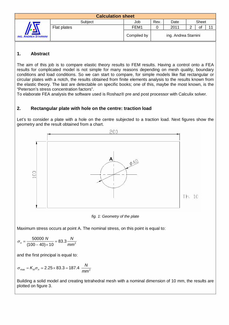
Let’s to consider a plate with a hole on the centre subjected to a traction load. Next figures show the geometry and the result obtained from a chart.

fig. 1: Geometry of the plate

Maximum stress occurs at point A. The nominal stress, on this point is equal to:

2

50000 83.3(100 40) 10n

N Nmm

and the first principal is equal to:

max 22.25 83.3 187.4 tn nNK

mm

Building a solid model and creating tetrahedral mesh with a nominal dimension of 10 mm, the results are plotted on figure 3.


FEM1 0 2011 3 of 11


Flat plates


fig. 2: Stress concentration factor

fig. 3: Mesh 5 mm

Changing the mesh size around the hole from 10 mm to 5 mm the result are plotted on figure 4.


FEM1 0 2011 4 of 11


Flat plates


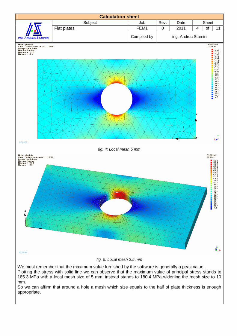
fig. 4: Local mesh 5 mm

fig. 5: Local mesh 2.5 mm

We must remember that the maximum value furnished by the software is generally a peak value. Plotting the stress with solid line we can observe that the maximum value of principal stress stands to 185.3 MPa with a local mesh size of 5 mm; instead stands to 180.4 MPa widening the mesh size to 10 mm. So we can affirm that around a hole a mesh which size equals to the half of plate thickness is enough appropriate.


FEM1 0 2011 5 of 11


Flat plates


fig. 6: Maximum principal stress plotted by lines to avoid peak value (local mesh 5 mm)

fig. 7: Maximum principal stress plotted by lines to avoid peak value (local mesh 10 mm)

In this case the model is not large and so we have studied the whole model without simplifications. Considering a quarter of model because of the symmetry of geometry and of the load, the results are plotted on figure 8.


FEM1 0 2011 6 of 11


Flat plates


fig. 8: Maximum principal stress on a quarter of model (Local mesh 5 mm)

Also in this case the result are closed to the result obtained from the theory.

3. Flat rectangular plate with shoulder fillet

Let’s to consider a flat plate with two symmetrical shoulder fillets that reduces the wide dimension. Also in this case the fillet represents a notch and around it there’s a stress concentration. From theory, based on dimensions represented on figure 9, the stress concentration factor is equal about to 1.845. So the maximum stress is equal to:

max90000 1.845 276.8 60 10tn n

NK MPa

fig. 9

The result from FEA analysis is represented in figure 10. The mesh size around the notch is equal to 5 mm.


FEM1 0 2011 7 of 11


Flat plates


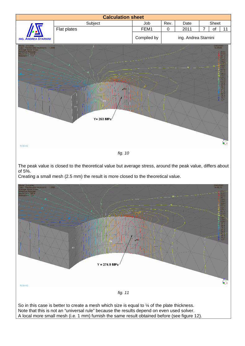
fig. 10

The peak value is closed to the theoretical value but average stress, around the peak value, differs about of 5%. Creating a small mesh (2.5 mm) the result is more closed to the theoretical value.

fig. 11

So in this case is better to create a mesh which size is equal to ¼ of the plate thickness. Note that this is not an “universal rule” because the results depend on even used solver. A local more small mesh (i.e. 1 mm) furnish the same result obtained before (see figure 12).


FEM1 0 2011 8 of 11


Flat plates


fig. 12

4. Flat rectangular plate with U-shapes

Now we consider a flat bar with two symmetrical U shapes which dimensions are depicted on figure 14. The bar is subjected to a traction force of 30 kN. The theoretical maximum stress is equal to:

max300003.02 151.0 120 5tg gK MPa

fig. 13

The stress concentration factors is calculated by an applet (see figure 14).


FEM1 0 2011 9 of 11


Flat plates



Creating a local mesh that locally is equal to half of the bar thickness, we obtain the result plotted on figure 15.

fig. 15

The peak value is closed to the theoretical value. The average value, around the peak, is less than the theoretical of 3%. So the FEA results is acceptable. Making a more small mesh (1 mm) the new result is plotted on figure 16.


FEM1 0 2011 10 of 11


Flat plates


fig. 16

The peak value and the average value are closed to the values obtained from the other analysis with a larger mesh. Also on this case a local mesh which dimension is equal to the half of plate thickness furnish a good result.

5. Flat plate with two holes

Now we are going to consider a plate with two holes of the same diameter and placed on the traction force direction.

fig. 17

Because of the wide dimension is larger that the holes diameter, we consider a case of two holes in infinite panel. The stress concentration factor is equal to 2.69. So, considering a traction force of 50 kN, the maximum principal stress is equal to:


FEM1 0 2011 11 of 11


Flat plates


max20000002.69 269.0 100 5

tg gK MPa


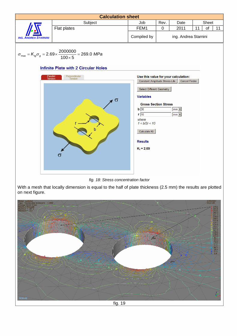
With a mesh that locally dimension is equal to the half of plate thickness (2.5 mm) the results are plotted on next figure.

fig. 19

Index: 1. Abstract2 2. Rectangular plate with hole on the ... · Flat rectangular plate with...

Documents

Transcript of Index: 1. Abstract2 2. Rectangular plate with hole on the ... · Flat rectangular plate with...