Indeterminate Structural Analysis - priodeep.weebly.com · 3.5 Application of Moment Distribution...
127
Transcript of Indeterminate Structural Analysis - priodeep.weebly.com · 3.5 Application of Moment Distribution...


INDETERMINATE TRUCTURAL ANALYSIS
Kenneth Derucher, Chandrasekhar Putcha and
Uksun Kim
The Edwin Mellen Press Lewiston•Queenston•Lampeter

Library of Congress Cataloging-in-Publication Data
Library of Congress Control Number: 2013934083
Derucher, Kenneth. Indeterminate structural analysis / Kenneth Derucher, Chandrasekhar
Putcha, Uksun Kim. 1. Mathematics--advanced. 2. Science--mechanics--dynamics--general. 3. Putcha, Chandrasekhar. 4. Kim, Uksun.
p. cm. Includes bibliographical references and index. ISBN-13: 978-0-7734-4470-6 (hardcover) ISBN-10: 0-7734-4470-X (hardcover) I. Title.
hors serie.
A CIP catalog record for this book is available from the British Library.
Copyright 2013 Kenneth Derucher, Chandrasekhar Putcha, and Uksun Kim
All rights reserved. For information contact
The Edwin Mellen Press The Edwin Mellen Press Box 450
Box 67 Lewiston, New York
Queenston, Ontario USA 14092-0450
CANADA LOS 1 LO
The Edwin Mellen Press, Ltd. Lampeter, Ceredigion, Wales
UNITED KINGDOM SA48 8LT
Printed in the United States of America


Tahla of Contents
PREFACE
INTRODUCTION 1
CHAPTER 1- ANALYSIS OF STATICALLY INDETERMINATE STRUCTURES BY THE FORCE METHOD 3
1.1 Basic Concepts of the Force Method 3 1.1.1 List of Symbols and Abbreviations Used in the Force Method 4
1.2 Static Indeterminacy 4 1.3 Basic Concepts of the Unit Load Method for Deflection Calculation 6 1.4 Maxwell's Theorem of Reciprocal Deflections 7 1.5 Application of Force Method to Analysis of Indeterminate Beams 8
1.5.1 Sign Convention 9 1.5.3 Structures with Several Redundant Forces 16
1.6 Application of the Force Method to Indeterminate Frames 16 1.7 Application of Force Method to Analysis of Indeterminate Trusses 21 1.8 Summary 26 Problems 27
CHAPTER 2 - DISPLACEMENT METHOD OF ANALYSIS: SLOPE-DEFLECTION METHOD 29
2.1 Basic Concepts of the Displacement Method 29 2.2 Basic Procedure of the Slope-Deflection Method 30
2.2.1 Slope-Deflection Equations 30 2.2.2 Sign Convention for Displacement Methods 31 2.2.3 Fixed-End Moments 32
2.3 Analysis of Continuous Beams by the Slope-Deflection Method 32

2.4 Analysis of Continuous Beams with Support Settlements by the Slope- Deflection Method 36
2.5 Application of the Slope-Deflection Method to Analysis of Frames Without Joint Movement 41
2.6 Derivation of Shear Condition for Frames (With Joint Movement) 45
2.7 Application of the Slope-Deflection Method to Analysis of Frames With Joint Movement 46 2.8 Summary 49
Problems SO
CHAPTER 3 - DISPLACEMENT METHOD OF ANALYSIS: MOMENT DISTRIBUTION METHOD 53
3.1 Basic Concepts of Moment Distribution Method 53
3.2 Stiffness Factor, Carry-Over Factor and Distribution Factor 54 3.2.1 Stiffness Factor 54 3.2.2 Carry-Over Factor (CO) 55 3.2.3 Distribution Factor (DF) 55
3.3 Analysis of Continuous Beams by Moment Distribution Method 57 3.3.1 Basic Procedure for Moment Distribution 57
3.4 Analysis of a Continuous Beam with Support Settlement by Moment Distribution Method 61
3.5 Application of Moment Distribution to Analysis of Frames Without Sidesway 65
3.6 Application of Moment Distribution to Analysis of Frames with Sidesway 68
3.6.1 Basic Concepts: Application of Moment Distribution to Analysis of Frames with Sidesway 68
3.7 Summary 78
Problems 79

CHAPTER 4- DIRECT STIFFNESS METHOD: APPLICATION TO BEAMS 81 4.1 Basic Concepts of the Stiffness Method 81 4.2 Kinematic Indeterminacy 81
4.3 Relation Between Stiffness Method and Direct Stiffness Method 82
4.4 Derivation/Explanation of the Beam-Element Stiffness Matrix 82 4.4.1 Global/Structure Stiffness Matrix 86
4.5 Application of the Direct Stiffness Method to a Continuous Beam 86 4.5.1 Basic Procedure of the Direct Stiffness Method for Beams 86
4.6 Summary 93 Problems 94
CHAPTER 5- DIRECT STIFFNESS METHOD: APPLICATION TO FRAMES 95 5.1 Derivation/Explanation of the Stiffness Matrix for a Frame Element 95 5.2 Application of the Direct Stiffness Method to a Frame 97 5.3 Summary 102 Problems 103
CHAPTER 6- DIRECT STIFFNESS METHOD: APPLICATION TO TRUSSES 105 6.1 Derivation/Explanation of the Stiffness Matrix for a Truss Element 105 6.2 Application of the Direct Stiffness Method to a Truss 107 6.3 Summary 111 Problems 112
APPENDIX — A 113 REFERENCES 114


?ire ace
The title of this book is "Indeterminate Structural Analysis", not
"Structural Analysis" as most of the books on this subject are titled. Many
textbooks have been written on structural analysis over the past several years
with a twofold composition. They essentially deal with analysis of statically
determinate structures followed by analysis of statically indeteuninate
structures using the force method, displacement methods (classical methods
such as slope-deflection and moment distribution) and the stiffness method.
Thus, the material covered in existing textbooks on structural analysis contains
more than what is necessary to learn indeterminate structural analysis. As a
result, these books become bulky and all their material cannot, and need not,
be covered in a single course on indeterminate structural analysis. Moreover,
these books rarely include an as-needed discussion of the unit load method,
which is arguably the best method to calculate deflections when solving
problems by the force method. Hence, the authors set out to create this book.
This book covers the analysis of indeterminate structures by force
method, displacement method and stiffness method in a total of six chapters.
The first chapter deals with application of the force method to analysis of
beam, frame and truss structures. The unit load method is discussed with
reference to the analysis of statically indeterminate structures. A few examples
are discussed to illustrate these concepts. The second and third chapters deal
with analysis of indeterminate structures by displacement methods. In the
second chapter, concepts of slope-deflection method are developed and applied
to beam and frame structures. The third chapter deals with developments of
concepts of the moment distribution method. These concepts are then applied
to beam and frame structures. The fourth chapter develops the concepts of the
stiffness method. These are subsequently applied to beam structures. The fifth

ii
Preface
and sixth chapters deal with application of the stiffness method to frame and
truss structures. Throughout the book, few but illustrative examples are
discussed under each method. The intent is to cover as much material as is
needed conceptually with minimal, yet sufficient, examples so the student can
understand indeterminate structural analysis methods without being
overwhelmed. This way, the book is kept less bulky compared to existing
books on structural analysis. In addition, keeping the textbook concise will
reduce the price far below that of existing textbooks, saving money for
students. We believe this will be a big selling point because the amount of
material covered is not compromised in covering the material in a concise
manner. This is in addition to the fact that, this book is written by three
Professors of Civil Engineering who have had vast experience in teaching and
research in the area of structural analysis.
It is hoped that this experience is reflected in the write-up of this book
so that it serves our twofold objective. The first objective is that we hope the
instructor following this book as a textbook for his/her course on indeterminate
structural analysis feels that all the required material is indeed covered in this
textbook. Secondly, we hope that the students taking this course find the book
and material covered easy to understand.
The authors are thankful to Mr. Kyle Anderson and Mr. AnhDuong Le,
former graduate students in the Department of Civil and Environmental
Engineering at California State University, Fullerton for going through the
manuscript and making constructive comments. We also appreciate the editing
work done by Mr. Alexander Motzny, undergraduate student in the
Department of Civil and Environmental Engineering at California State
University, Fullerton.
KENNETH DERUCHER
CHANDRASEKHAR PUTCHA
UKSUN KIM

li- :i.oducrdon
In structural analysis, there are three basics types of methods used for
analyzing indeterminate structures. They are:
1. Force Method (Method of Consistent Deformation)
2. Displacement Methods (Slope-Deflection and Moment Distribution)
3. Stiffness Method
General idea about these methods:
The force method of analysis is an approach in which the reaction
forces are found directly for a given statically indeterminate structure. These
forces are found using compatibility requirements. This method will be
discussed with more detail in Chapter 1.
The displacement methods use equilibrium requirements in which the
displacements are solved for and are then used to find the forces through force-
displacement equations. More on these methods can be found in Chapters 2
and 3.
The stiffness method is also considered a displacement method because
the unknowns are displacements, however the forces and displacements are
solved for directly. In this book, it will be considered separately due to
procedural differences from the other displacement methods. The stiffness
method is very powerful, versatile, and commonly used. This method will be
discussed in Chapters 4, 5, and 6.


Chapter 1
Analysis of Statically Indeterminate Structures by the Force Method (Flexibility Method or Method of Consistent Deformation)
1.1 Basic Concepts of the Force Method
The force method (which is also called the flexibility method or the
method of consistent deformations) uses the concept of structural Static
Indeterminacy (SI). It is very conceptual in nature. The force method becomes
cumbersome when the Static Indeterminacy of a structure is large. The results
obtained by solving the problem using the force method, are all the unknown
forces (such as reactions at the supports).
If one is interested in finding rotational or translational displacements of
an indeterminate structure, they must be obtained separately using any methods
of finding displacements (unit load method, moment area method or conjugate
beam method for example).
This method is applicable for any kind of structure: beam, frame or truss.
It is to be noted that beam and frame structures are predominantly bending
(flexure) structures while trusses are predominantly direct stress structures
(tension or compression) in nature. The truss members are not subjected to
bending. In other words, all loads are axial.

4
Chapter 1 — The Force Method
1.1.1 List of Symbols and Abbreviations Used in the Force Method
Symbols and terms are defined along with equations. However, some are not in
equations so they are defined below:
(LA)L: Deflection at point A due to applied loading
(DA)R: Deflection at A due to redundant loading RA * Saa
aaa: Rotational deflection at A due to a unit load at A
OA : Rotational deflection at A due to applied loading
6.: Deflection at A due to a unit load at A
1.2 Static Indeterminacy
The Static Indeterminacy (SI) for beams and frames is defined as,
SI = nu — ne
Where, nu = Number of unknown support reactions
Tie = Number of equations of equilibrium
In general for a two-dimensional structure, there are three equations of
equilibrium (ne = 3) and for a three-dimensional structure there are six
(ne = 6). The static indeterminacy refers to the number of reactions that are
unsolvable using basic statics.
This implies that a structure is statically determinate if SI = 0. An
example of this would be a simply supported beam (one end pinned and the
other having a roller support). This structure would have three unknowns, the
reactions at the pin in both the x and y directions and the reaction at the roller
in the y direction. The number of equilibrium equations would be three
(EF, = 0, EFy = 0, and >M = 0). Therefore SI = 0.

Chapter 1 — The Force Method 5
If SI > 1, the structure is said to be statically indeterminate to that
degree (value of SI), therefore the degree of Static Indeterminacy is equal to
the value of (nu — rte ). It can be also said that the structure has "SI" number of
redundants.
To solve a statically indeterminate beam (or frame) using the force
method we will make use of redundant forces. A redundant force is one, which
cannot be solved using static equilibrium equations alone. The forces will be
taken out and reapplied so that the considered structure is always statically
determinate. Additionally, the principle of superposition is applied and
deflection will be found as an intermediate step to solving for a given
redundant. This process will be further explained in the text along with
examples.
For a truss, static indeterminacy involves both external and internal
indeterminacy because of the internal members in a truss.
Static indeterminacy (SI) in the case of a truss is defined as,
SI = b + r — 2j
(1.2)
Where, b = Number of members in the truss
r = Number of reactions at the supports
j = Number of joints in the truss
The analysis of an indeterminate structure is split into a series of
determinate structures acted on by applied loads (in the original structure) and
acted on by redundant force(s). In both cases the deflections need to be found.
Hence, the unit load method for finding deflection will be discussed briefly for
a determinate structure.

6 I Chapter 1— The Force Method
1.3 Basic Concepts of the Unit Load Method for Deflection Calculation
The unit load method is also referred to as the method of virtual work.
The basic equation to calculate displacement (whether translational or
rotational) at a given point of a beam or frame is given as,
M m dx A = f
El (1.3)
Where, M Moment at any point in a structure due to applied loads
m Moment at any point in a structure due to the unit load (force or
moment) at the point of interest corresponding to the parameter
of interest (deflection or rotation)
E Modulus of elasticity
I Moment of inertia of the cross section of a member
Note: The above equation has been derived using energy principles.
To find in, the applied loads are removed and a unit load (force or
moment) is applied at the point of interest, or redundancy, in a structure. If one
is interested in finding a vertical deflection at a point in a structure, then a unit
vertical force is applied (as it corresponds to vertical deflection). If one is
interested in finding horizontal deflection at a point, then a unit horizontal
force is applied at that point as it corresponds to horizontal deflection.
Similarly, rotational displacement at a point in a structure is found by applying
a unit moment as it corresponds to rotation.
Chapter 1 — The Force Method 7
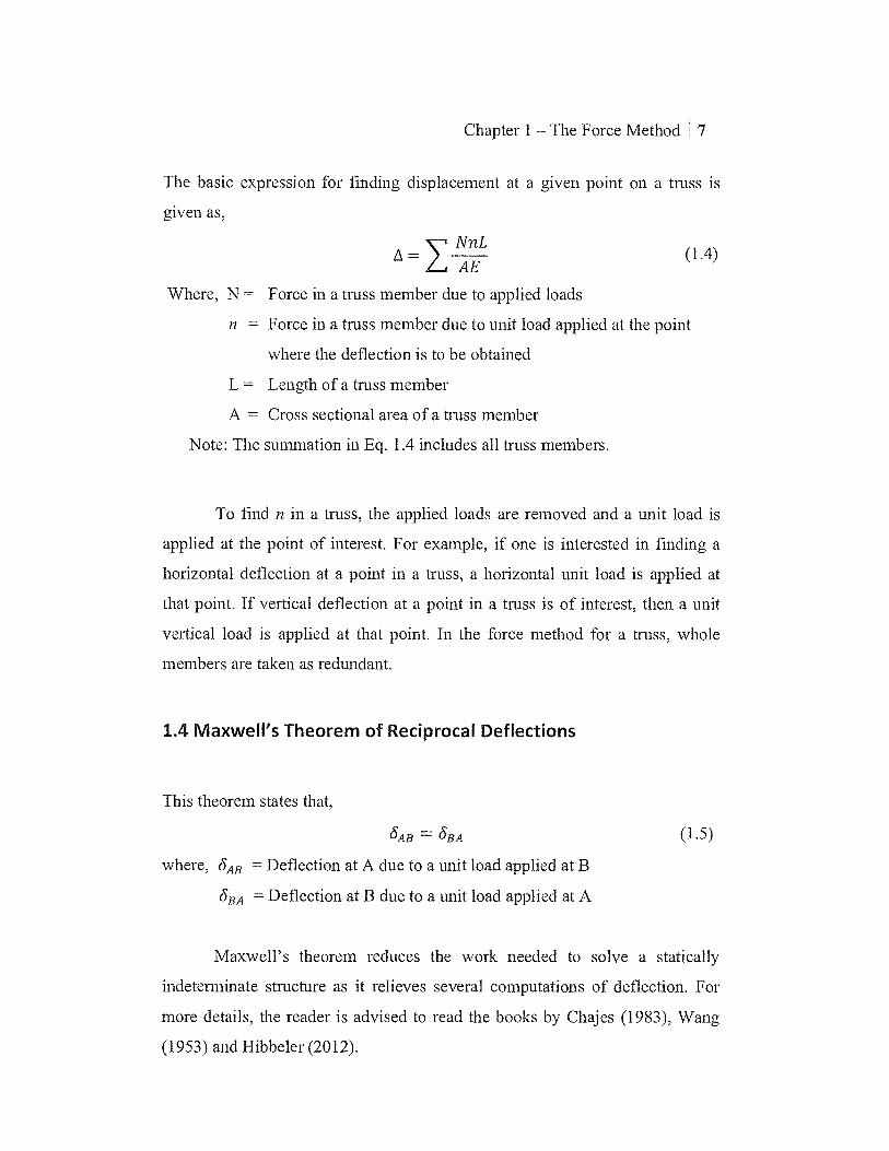
The basic expression for finding displacement at a given point on a truss is
given as,
v AE NnL
(1.4)
Where, N = Force in a truss member due to applied loads
n = Force in a truss member due to unit load applied at the point
where the deflection is to be obtained
L = Length of a truss member
A = Cross sectional area of a truss member
Note: The summation in Eq. 1.4 includes all truss members.
To find n in a truss, the applied loads are removed and a unit load is
applied at the point of interest. For example, if one is interested in finding a
horizontal deflection at a point in a truss, a horizontal unit load is applied at
that point. If vertical deflection at a point in a truss is of interest, then a unit
vertical load is applied at that point. In the force method for a truss, whole
members are taken as redundant.
1.4 Maxwell's Theorem of Reciprocal Deflections
This theorem states that,
SAB = SBA (1.5)
where, b' AB = Deflection at A due to a unit load applied at B
SBA = Deflection at B due to a unit load applied at A
Maxwell's theorem reduces the work needed to solve a statically
indeterminate structure as it relieves several computations of deflection. For
more details, the reader is advised to read the books by Chajes (1983), Wang
(1953) and Hibbeler (2012).

8
Chapter 1 — The Force Method
1.5 Application of Force Method to Analysis of Indeterminate Beams
1. Calculate the Static Indeterminacy (SI) of the structure using Eq. 1.1 or
Eq.1.2 depending upon whether the structure is beam, frame, or truss.
2. Choose one of the reaction forces (or internal members of the truss) as
the redundant force. One at a time if there are multiple redundancies.
3. Split the statically indeterminate structure into a determinate structure
(acted upon by applied loads on the structure) and determinate
structure(s) acted on by the redundant forces (one at a time).
4. Analyze the determinate structures by the unit load method to find the
displacement AL, which is the displacement for the applied loading and
redundant removed. Then find 8, which is the displacement for the unit
load only, at the point of redundancy. If a moment is taken as
redundant, the corresponding displacements will be 0 and a.
5. Finally, formulate equation(s) of displacement compatibility at the
support(s) (in the case of beams and frames). In the case of trusses,
displacement compatibility of truss bars will be used.
6. Solve these equation(s) to get the redundant force(s).
7. Calculate all the reactions at the supports (in addition to the redundant
force already determined in step 6) using principles of statics.
A total of 3 examples are solved in this chapter: one for a statically
indeterminate beam, one for a statically indeterminate frame, and one for
statically indeterminate truss. While any of the methods for finding deflection
(double integration, moment area method, conjugate beam method, unit load
method, or any other existing method) can be used to find displacements

Chapter 1 — The Force Method ; 9
(translation or rotation), the authors recommend use of the unit load method
because it is conceptually straight forward and easy to use.
1.5.1 Sign Convention
The following sign convention will be used for the force method:
• Counter-clockwise moments and displacements are positive
This is often referred to as the right hand rule.
When a member undergoes bending:
• Compression on a member's top fiber is positive bending
• Compression on a member's bottom fiber is negative bending.
• _ ____________
a) Positive bending -top fiber compression
b) Negative bending -bottom fiber compression
Figure 1.1: Bending sign convention

10 I Chapter 1 — The Force Method
1.5.2 Example of an Indeterminate Beam
An example dealing with the analysis of a statically indeterminate beam using
the force method is solved below.
Example 1.5.2.1
Determine the reactions at the supports for the statically indeterminate structure shown in Fig. 1.2 by the force method. Use RB as the redundant. Take E = 29000 ksi and I = 446 in4.
36k
A
B
C
10ft
12ft
Figure 1.2: Statically indeterminate beam

Chapter 1 — The Force Method 1
Solution:
A
loft 12ft
a) Actual beam
36 k
C Actual Beam
36 k
Primary Structure
b) Primary structure
RB
Redundant RB applied
RBC5BB
c) Redundant RB applied
Figure 1.3: Two determinate structures
The given indeterminate structure is split into two determinate
structures as shown in Fig. 1.3b and 1.3c choosing RB as the redundant force.
The basic equation used is as given in Eq. 1.3. This is stated again below:
M m dx El
The procedure will be followed as it is stated earlier in this section.
Step 1.
(1.3)
S/ = u — ne = 4 — 3 = 1
Step 2
Choose RB as the redundant force (in the problem statement).

12 I Chapter 1 — The Force Method
Step 3
The two determinate structures are shown below with Fig. 1.4a
acted on by the applied loading, and Fig. 1.4c acted on by the redundant
force RB (unit load). The deflection at B for the statically determinate
structure (LX B)L due to applied loads can be obtained from Eq. 1.3 using the
values of M and in. Figures 1.4a — 1.4d are used to calculate M and in.
Redundant removed, applied loading Redundant applied with unit magnitude
36k 1 k
A
B
A C
B
x x x x
a) FBD for M c) FBD for m 36k 1k
792 k-ft t_ 10 k-ft
Figure 1.4: FBD for M and in (AB) and cut sections
The values for M and in will depend on the origin chosen and the
corresponding change in limits. In doing this, it may simplify the
integration and the final value of deflection will be the same.
Step 4
Deflection at B due to the applied loads
The required values for calculation of deflection are tabulated in. Table 1.1.
Table 1.1: Calculation of deflection using Fig. 1.3a and b Portion of the beam AB BC Origin A C Limit x = 0 to x = 10 x = 0 to x = 12 M 36x — 792 —36x m x — 10 0
36k
C
x x
b) Cut section for M
C x x
d) Cut section for in

Chapter 1 — The Force Method 13
Calculate M
Portion AB:
Reaction forces: RA = 36 k and
MA = 36 * (10 + 12) = 792k-f t
Equilibrium equation:
M + 792- 36x = 0 —> M = 36x — 792
Portion BC:
Equilibrium equation: —M- 36x = 0 —> M = —36x
Calculate in
Portion AB:
Reaction forces: RA = 1k and MA = 1 * 10 = 10k-ft
Equilibrium equation: m + 10- x = 0 —> m = x — 10
Portion BC:
Equilibrium equation: m = 0
It is to be noted that the value of M (shown in Table 1.1) is
calculated using Fig. 1.4a & 1.4b while the value of ni is calculated from
Fig. 1.4c & d. The determinate structure shown in Fig. 1.4c is the same
determinate structure as shown in Fig. 1.4a but acted on by a unit
downward load at B (with no given applied loads) as it is assumed that the
vertical deflection at B is downward. If at the end of the calculation, the
deflection at B comes out to be positive, that means the actual deflection is
downward. On the other hand, if the final deflection at B comes out to be
negative, it means that the actual deflection at B is upward.
Substituting the values of M and 171 (from Table 1.1) in Eq. 1.3, the
deflection (AB) L (deflection at B due to the applied loads) is calculated as,
AB= E f Mm = f1°(36x — 792)(x — 10)dx El El 0 (1.6)

14 I Chapter 1 — The Force Method
33600 AB=
El
(1.7)
The deflection at B due to a unit value of the redundant force RB (ebb) is obtained from Fig. 1.5 as shown in Table 1.2 below.
1k
A B
x x
a) FBD for m
M=m M=m
A
C
b) Cut section for in x
Figure 1.5: FBD for m (obb) and cut section
Table 1.2: Calculation of deflection using Fig. 1.4 Portion of the beam AB BC Origin A C Limit x = 0 to x = 10 x = 0 to x = 12 M = m x — 10 0
Substituting the values of M and m (M = m) in eq. 1.3,
8bb = "M -
dx
= 1010 (x — 10)(x — 10)dx (1.8)
El El
The deflection at B due to a unit value of the redundant force (RB) is
obtained as,
ebb = 3E1 1000 (1.9)
Step 5
Equation of compatibility of displacement at joint B requires that,
(LB)L — ('AR = 0 (1.10)
Where,
1k
10 k-ft
(LB)R RB * (ebb)

Chapter 1 - The Force Method 15
This equation is essentially saying, the total vertical displacement at B has
to be zero as it is a roller joint.
Substituting the values of (MI, and aibb) calculated above, Eq.
1.10 can be rewritten as, 33600 1000 + RB X = 0 El 3E1
Step 6
Solving Eq. 1.11 above, RB can be obtained as,
RB = -100.8k T
This shows that RB is upward, not downward, as assumed in Fig. 1.3c.
Step 7
Once the redundant force (RB) is obtained, then the remaining
reactions at A (RA and MA ) can easily be obtained from equilibrium
equations.
They are calculated using Fig. 1.6 as,
E Ty = 0 Ay + 100.8 - 36 = 0 Ay = -64.8 k
EWA = 0 MA + 100.8(10)- 36(22) = 0 -4 MA = -2161{-ft ZJ
Ay
---- MA B
36 k
C
Ax
^.0 10 ft 12 ft
Figure 1.6: Final reactions for the indeterminate beam

16 Chapter 1 — The Force Method
It has been shown above by solving a simple example that when
solving a statically indeterminate structure by the force method; first, write the
correct expressions for M and in, and then integrate the expression to solve for
deflection within the specified limits (consistent with the chosen origin).
1.5.3 Structures with Several Redundant Forces
As stated earlier, it is to be noted that if a structure has several
redundant forces (i.e. S/ > 1), then indeterminate structural analysis of the
structure would involve obtaining redundant forces through solution of
simultaneous equations. This will be followed by obtaining the remaining
reactions at the supports (other than the redundant forces) through principles of
statics as done in Ex. 1.5.2.1.
The reader is advised to see other literature for detailed information
such as those found in the references of this book.
1.6 Application of the Force Method to Indeterminate Frames
The basic procedure for analysis of statically indeterminate frames
essentially remains the same as outlined in Sec. 1.5, and as illustrated for a
beam in Example 1.5.2.1 in Sec. 1.5.
Although the analysis of an indeterminate frame is, conceptually, very
much similar to that of the beam, a frame consists of beams and columns so the
analysis is slightly more complicated. After following the example below, it
will be clear how to apply the force method to indeterminate frames.

Chapter 1— The Force Method 17
1.6.1 Examples of an Indeterminate Frame
A structural analysis dealing with a statically indeterminate frame by the force
method is shown below in Example 1.6.1.
Example 1.6.1.1
Determine the reactions at the supports of the frame shown in Fig. 1.7 using the force method. A = 100 in2, E = 29000 ksi and I = 833 in4.
4 k/ft
A
8 ft
10 ft
Figure 1.7: Statically indeterminate frame
Solution
The procedure followed is as stated in Sec. 1.5.
Step 1
S/ = nu- ne = 4 — 3 = 1
Step 2
Choose MA as the redundant moment.
Step 3
The given statically indeterminate structure is split into two
determinate structures as shown in Fig. 1.8, with the redundant moment
removed and with the applied loading as shown in Fig. 1.8b. In Fig. 1.8c,
the frame is acted on by the redundant moment MA. The rotational
deflection at A due to applied loads is OA, and due to the unit load, MA, is

18 Chapter 1 — The Force Method
MA xaAA. These rotations can be obtained from Eq. 1.3 by finding the
values of M using Fig. 1.8b and respective values of m using Fig. 1.8c. In
both cases HA and VA are found using static equilibrium equations.
Note on symbols: In general, (04 HAHA) represents the horizontal deflection
at A due to a unit horizontal unit load at A (i.e. HA = 1). Similarly,
(SVAHA) represents the vertical deflection at A due to a unit horizontal
unit load at A. Along the same lines, (SHAVA) and ( ,6vAvA) represent
the horizontal and vertical deflection at A respectively due to a unit
vertical load at A (i.e. VA = 1).
Note: The values for M and m will depend on the origin chosen (with the
corresponding change in limits). As can be expected, the final value of
deflection will be the same irrespective of how it is done.
This frame is statically indeterminate to the first degree. Since we
chose the moment reaction at A as the redundant, the support at A will
become a pin as seen in Fig. 1.8.
4 k/ft
4 k/ft
MA
OA
HA A A MAann
8 ft
10ft
VA
a) Actual frame b) Primary structure c) Redundant MA applied
Figure 1.8: Given indeterminate and corresponding determinate structures
Applying the principle of superposition to the frame yields:
— MA * aAA = (1.12a)

Chapter 1 — The Force Method 19
In this case, both 0A and MA * aAA are negative because they both
create a clockwise rotation at joint A. This is negative by the sign
convention defined in section 1.5.1. Equation 1.12 can also be written as:
9A + MA * aAA = (1.12b)
Eq. 1.12b can also be found by considering that both 6A and MA * aAA
create compression at the top fiber of member AB.
Step 4
Use the unit load method to calculate OA:
4 k/ft
B
x
m
, x
A C 16 k
+8k
a) Applied loads b) Unit load MA
Figure 1.9: Bending moments due to applied and unit loads
dx 1 Et —4
6A = f Mine—
r = (16x — 2x2) (1 — dx = 256
El El 0 8 3E1
Use virtual work (unit load method) to calculate aAA:
Table 1.3: Deflection calculation for Portion of the beam AB BC Origin A C Limit x = 0 to x = 8 x = 0 to x = 10 M 16x — 2x2 0
1710 x
1— —8
0
A
16k
k-ft
B
x

20 I Chapter 1 - The Force Method
Table 1.4: Deflection calculation for a Portion of the beam AB BC Origin A C Limit x = 0 to x = 8 x = 0 to x = 10
M = me x
1 - -8 0
2 dx 1 i8 aAA f memo El = El = J O - -8) dx 3E1
Step 5
Equation of compatibility:
OA + MA * aAA = 0 Step 6
Plugging in the values for deflection: 256 8 —3E1 +M- A (3E1) = 0-* MA = -32k-ft 0
Here, MA is negative, which indicates that the moment is opposite to
clockwise assumed direction of MA in Fig. 1.8c.
Step 7
Use static equilibrium equations to calculate the remaining support
reactions:
= 0 H A =
MA 32(4) + 17c(8) = 0 = 12 k T
+TETy = 0:
VA + 12 - 32 = 0 V A = 20 k T

Chapter 1 — The Force Method 21
4 k/ft
" 1<-"—A iiiiiiiiii
20 k
12 k
Figure 1.10: Final reactions and moments for the indeterminate frame
This completes solution of the problem.
1.7 Application of Force Method to Analysis of Indeterminate
Trusses
The analysis procedure for a statically indeterminate truss follows the
same lines of beams and frames, discussed in Sec. 1.3. The basic equation used
for calculating deflection is given by Eq. 1.4 and stated here again as,
A = NnL v AE
(1.4)
An example dealing with the analysis of a statically indeterminate truss is
solved in Example 1.7.1.

3ft
22 I Chapter 1 — The Force Method
Example 1.7.1
Determine the reactions at the supports of the truss shown in Fig. 1.11 using the force method. AE is constant.
4ft
A
4k
Figure 1.11: Statically indeterminate truss
Solution
Step 1
Degree of indeterminacy = b + r — 2j
= 3 + 4 — 2(3) = 1
Step 2
Choosing BC as the redundant, this member will be "cut" to make the truss
statically determinate.
Step 3
The given statically indeterminate structure is split into two
determinate structures as shown in Fig. 1.12. Fig. 1.12b shows the structure
under the given loading, and Fig. 1.12c shows the truss with the redundant
unit load applied.

Chapter 1 — The Force Method 23
C
IF BC BC
_ I FBC8BC
Fsct A B A B B A
4k 4k !i
a) Actual Truss b) Primary structure c) Redundant FBC
Figure 1.12: Statically indeterminate and corresponding determinate trusses
Applying the principle of superposition to the truss yields:
FBC * 8BC °
(1.13)
Step 4
Use the unit load method to calculate ABC:
Calculate N and 17 for each member in both cases: real load and virtual unit
load as is shown in Fig. 1.13.
-FIEF; = 0:
—4 + FAc = 0 F Ac = 5 k (T)
--> = 0:
FAR F Ac = 0
F AB = —3 k (C) 4 k
a) Calculation of FAR and F Ac
applied

24 I Chapter 1 — The Force Method
5k 0 ir 1k
0 1 k t
B A 0
b) Calculation of N c) Calculation of n
Figure 1.13: Calculation of forces for N and it
ABC = ""dv nANEL - Ct(A5; "A—E3)3
▪
1(0)4
)4 o
Use the unit load method to calculate SBC:
8BC = n2 L 02(5)
+ 02(3) 12 (4) 4-
AE AE AE AE AE
Step 5
The compatibility equation given by Eq. 1.13 is repeated below.
/IBC + FRC * 8I3C =°
(1.14)
(1.15)
(1.13)
Step 6
From equation (1.13) —4 0 + FBc * —A4E = 0 Fgc = 0
Using this result, the forces in other members and the support reactions can
be calculated easily using the method of joints.

Chapter 1 — The Force Method 25
Step 7
The method of joints for B and C along with the final reactions are shown
below in Fig. 1.14:
5 k Ok
-FTEFy = 0: C 5(.4:•) = Y 5 Cy = 4 k T
+ 5(i) = Cx = 3 k
+11T;, = 0: —By + 0 = 0 B = O
ETX = 0:
B, — (-3) = 0
B, = —3 k
a) Calculation of C, and Cy b) Calculation of Bx
3k
5k
B 3k A
-3k 4 k!
c) Final reactions
Figure 1.14: Final reactions and internal forces for the indeterminate truss

26 I Chapter 1 — The Force Method
1.8 Summary
In this chapter, the basic concept of the force method is explained
briefly but succinctly. This is followed by application of the force method to a
set of problems dealing with structural analysis of an indeterminate beam,
frame and truss. It is to be noted that force method uses the concept of Static
Indeterminacy (SI) and involves a large number of deflection calculations.
Hence, knowledge of the prerequisite courses dealing with deflection
calculations is paramount to a strong understanding of this approach.

Chapter 1 — The Force Method 127
Problems
Analyze the Problems from 1.1 to 1.3 for all the unknown reactions using the
force method.
Problem 1.1 Determine the reactions at the supports of the beam shown in
this figure. EI is constant.
8 m • 4 m
Problem 1.1
Problem 1.2 Determine the reactions at the supports of the frame shown in
this figure. EI is constant.
8k
10 ft
L_.
B 2 4 ft
6 ft
8 ft
Problem 1.2

28 Chapter 1 — The Force Method
Problem 1.3 Determine the reactions at the supports of the truss shown in
this figure. AE is constant.
4m Problem 1.3

Chapter
Displacement Method of Analysis: Slope-Deflection Method
2.1 Basic Concepts of the Displacement Method
The displacement method refers to the general approach of solving
indeterminate structural analysis problems with displacements as the primary
variables. Two displacement methods that will be explained in this book are
classical methods called slope-deflection and moment distribution. The
displacement method uses the concept of structural Kinematic Indeterminacy
(KI). The formula for this is:
K.I. = (degrees of freedom at all supports in the given structure) (2.1)
Where: Degrees of freedom are unrestrained motions of a joint/support. This means a fixed support has zero degrees of freedom and a pin has one (rotation).
The results obtained using the slope-deflection method are the end
moments (internal moments) at the supports of the structure. These are found
through a two-step process of first finding the rotations (slopes), and second
finding the end moments. In contrast, the moment distribution method, which
will be discussed in Chapter 3, gives end moments directly as a result of the
procedure. After finding the end moments, the reactions at various supports
can be determined using principles of statics.
In the slope-deflection method, the unknown displacements are usually
rotational displacements of a pin or roller support. The displacements are
written in terms of the loads using the load-displacement relationships, also
known as slope-deflection equations. The resulting equations are then solved

30 Chapter 2 — Slope-Deflection
for the displacements. Therefore, the main intermediate output resulting from
the slope-deflection method is displacements. The final output is end moments.
2.2 Basic Procedure of the Slope-Deflection Method
2.2.1 Slope-Deflection Equations
Before the actual procedure is discussed, it is important to introduce the
slope-deflection equations, which are key to the slope-deflection method.
Derivation of the slope-deflection equations will not be shown; these are done
with great detail in the books listed in the references section.
L
MBA
a) Beam Fixed at B
b) Beam Fixed at A
L
c) Beam with support settlement
Figure 2.1: Moments and displacements on typical indeterminate beams

Chapter 2 — Slope-Deflection 31
With respect to Fig. 2.1, the slope-deflection equations can be written (without
support settlement) as,
MAB = MFAB 2E1
(29A + GB)
(2.2)
2E1 MBA = MFBA (20B + BA)
(2.3)
Wang (1953) advocates using relative stiffness factors instead of actual
stiffness factors to simplify the calculations. Modifying Eq. 2.2 and Eq. 2.3 to
include stiffness factors yields,
MAB = MFAB KAB(29A + 9
•
B)
(2.2a)
MBA = MFBA KBA(26B + O
•
A)
(2.2b)
Where, MAB MBA MFAB
MFBA
OA
= Moment at joint A of member AB = Moment at joint B of member AB = Fixed-end moment at end A of member AB due to
applied loading = Fixed-end moment at end B of member AB due to
applied loading = Slope at joint A = Slope at joint B
2.2.2 Sign Convention for Displacement Methods
• Clockwise moments are positive
▪ Counterclockwise moments are negative
• Clockwise rotations are positive
• Counterclockwise rotations are negative

32 Chapter 2 — Slope-Deflection
2.2.3 Fixed-End Moments
Fixed-end moments are reactionary moments of a single span beam
having fixed supports for a given loading. Table 1A give fixed-end moment
values for various load types.
2.3 Analysis of Continuous Beams by the Slope-Deflection
Method
Before discussing examples, the calculation procedure will be outlined below:
1. Calculate all the fixed-end moments due to applied loads at the end of
each span using Table lA found in the appendix.
2. Calculate the Kinematic Indeterminacy (KI) of the structure. It is
expressed as,
K.I. = E (degrees of freedom at all supports in the given structure)
Degrees of freedom are unrestrained motions of a joint/support. This
means a fixed support has zero degrees of freedom, a pin has one
(rotation), and a frame's joint has one (rotation).
3. Formulate all the slope-deflection equations for each member of the
continuous beam using Eq. 2.2 and Eq. 2.3. These equations are in
terms of the unknown rotations at the supports.
4. Formulate simultaneous equilibrium equations at the joints (not fixed)
using the basic premise that the sum of the end moments at the support
(for all the members joining at the support) is zero. The number of
unknown rotations in the problem is equal to the number of
simultaneous equations to be solved as well as the KI found in step 2.
5. Solve the simultaneous equations formulated in Step 4 and obtain
rotations at the supports.

Chapter 2 — Slope-Deflection 33
6. Compute end moments by substituting rotations back into the slope-
deflection equations.
7. Depending on the statement of the problem, calculate all the reactions.
8. Draw shear and moment diagrams for the continuous beam as needed.
Example 2.3.1
Determine the reactions at the supports for the statically indeterminate beam shown in Fig. 2.2 by the slope-deflection method. Take E = 29000 ksi and I = 446 in4.
36 k
A
I
C
10 ft
12 ft
Figure 2.2: Statically indeterminate beam
Solution
Step 1
Calculate the fixed-end moments using Table 1A found in the
appendix. The fixed-end moments for AB and BA are both zero because
there is no loading on the span of member AB.
MFAB =7- 0 and MFBA = 0
Step 2
KI =1
The unknown displacement is OB. Although the other unknown
displacements (0c and Ac) exist, these displacements are unnecessary to
CT'

34 Chapter 2 - Slope-Deflection
solve the problem because they do not occur at a support where specific
unknowns need to be found (B y) . 6B must be found so that we can find the
reaction at B. In contrast, solving for Oc would not give us any information
about the reactions of the structure.
Step 3
Slope-deflection equations are formed using Eq. 2.2 and Eq. 2.3 as,
/ , El al
B MAB 0 + L
„ E, - LLuA uBJ = — u 10 5
(Note: OA = 0 due to the fixed support at A)
MBA = 0 + 2E -1-1-0- [20B + OA] = 25E/ 9B
Similarly, MBC can be written as,
MBC =- 36 * 12 = -432k-f t
Note: MBC is negative because the internal moment caused by the loading,
acts in the counterclockwise direction (opposite to the external moment
at that point).
Step 4
Since KI = 1 for this problem, there is only one unknown, which is
OB. Hence, there is only one joint equilibrium equation to be solved. This
is given as,
MBA + MBC °
Step 5
Substituting the expressions for MBA and MBC from step 3, we have,
2E1 080 s OB- 432 = 0 --> =
1El
(2.4)
(2.5)
(2.6)
(2.7)
Chapter 2 — Slope-Deflection I 35
Step 6
Substituting the value of the rotation back into the slope-deflection
equations found in step 3, the end moments can be expressed as,
MAB = 216k- f t u
(2.8)
MBA = 432k- f t Z.) (2.9)
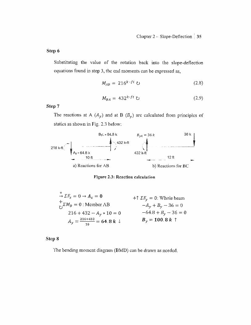
Step 7
The reactions at A (Ay) and at B (By) are calculated from principles of
statics as shown in Fig. 2.3 below:
216 k-ft Ay = 64.8 k
10 ft
Bye = 64.8 k
432 k-ft
ByR = 36 k 36 k
432 k-ft 12 ft
a) Reactions for AB b) Reactions for BC
Figure 2.3: Reaction calculation
—> EF, = 0 —* A, = 0 +T EFy = 0: Whole beam +EMB = 0 : Member AB —AY + BY — 36 = 0
216 + 432 — Ay * 10 = 0 —64.8+ By -36= 0
216+432 B = 100.8 k T Ay= 10 = 64.8 k
Step 8
The bending moment diagram (BMD) can be drawn as needed.

36 Chapter 2 — Slope-Deflection
2.4 Analysis of Continuous Beams with Support Settlements by the Slope-Deflection Method
The slope-deflection equations including settlement with respect to Fig. 2.4 are
given as, + _2LE/ (29A ,„„
k,LuA -r uB- MAB MFAB 3IFAB)
2E1 MBA = MFBA L (20B + OA- 37-1 BA)
(2.10)
(2.11)
Where, MAB = Moment at joint A of member AB MBA = Moment at joint B of member AB MFAB = Fixed-end moments at the end A of member AB due
to applied loading MFAB = Fixed-end moments at the end B of member AB due
to applied loading OA = Slope at joint A 0B = Slope at joint B TAB = Rotation of the member AB due to translation
(settlement) of joint B perpendicular to member AB
'TAB = A IL
(2.12)
Where, A = Translation (settlement) of joint B perpendicular to axis of member AB
L = Length of member AB
P
A
B
A ,
Figure 2.4: Statically indeterminate beam with support settlement at B

Chapter 2 — Slope-Deflection 37
It is to be noted that 'I' is treated positive when the rotation is
clockwise, consistent with the sign convention stated in Sec. 2.2.2.
Equations 2.10 and 2.11 can be rewritten using the relative stiffness
factors and relative TAB values as,
MAB = MFAB KAB(29A OB-34fre1)
(2.10a)
MBA = MFBA KBA(20B + 0A-34frei)
(2.11a)
The relative stiffness factors (KAB and KBA) for any general member AB can
be expressed as 2E1 /L and 'Frei as A /L.
The procedure for solving continuous beams where joints are subjected
to vertical translation amounting to settlement of supports remains the same as
discussed in Sec. 2.3.
Example 2.4.1
Determine the reactions at the supports for the statically indeterminate beam shown in Fig. 2.4 by the slope-deflection method. Take E = 29000 ksi and I = 446 in4. The support at B is displaced downward 1 in.
36 k
1 0 ft
12 ft
Figure 2.4(repeated): Statically indeterminate beam with support settlement at B

38 Chapter 2 - Slope-Deflection
Solution
Step 1
In the slope-deflection method, fixed end moments due to support
settlement are not considered because support settlement is accounted for
using II'.
MFAB = 0 and MFBA = 0
Step 2
KI = 1
Since IF is known, the only unknown displacement is OB. Moreover,
due to downward displacement at B, it can be seen that the cord of span
AB rotates clockwise, thus 'If is positive.
A
Figure 2.5: Effect of displacement at B
1 in 'FAB - LFBA 10(12) in
= 0.00833 rad
Step 3
Slope-deflection equations are formed using Eq. 2.10 and Eq. 2.11.
MAB = 0 + 2E [MA + B 31F AB] = (0 B- 3 * 0.00833)
MAB = 25 (9B- 0.025)
MBA = 0 + 2E io [28B + OA - 3111BA]= E. 2-5 (20B-3 * 0.00833)
Chapter 2 - Slope-Deflection j 39
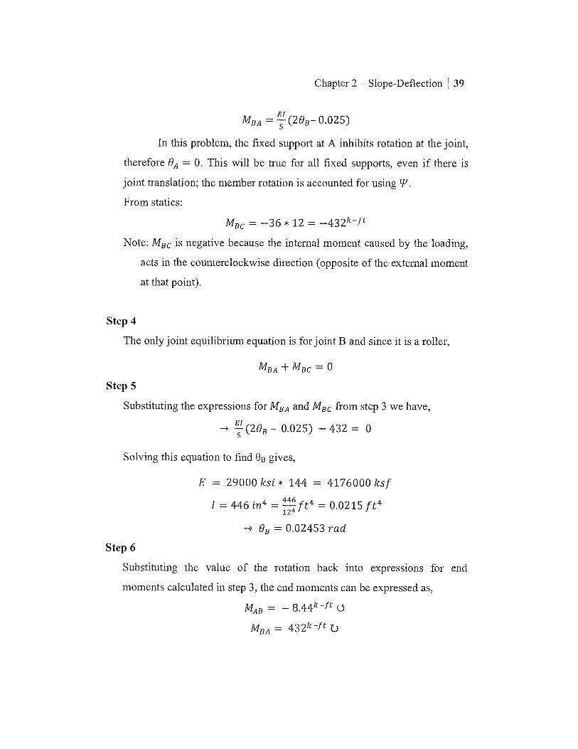
MBA = (29B- 0.025)
In this problem, the fixed support at A inhibits rotation at the joint,
therefore 0A = 0. This will be true for all fixed supports, even if there is
joint translation; the member rotation is accounted for using W.
From statics:
MBC = -36 * 12 = -432k-ft
Note: MBC is negative because the internal moment caused by the loading,
acts in the counterclockwise direction (opposite of the external moment
at that point).
Step 4
The only joint equilibrium equation is for joint B and since it is a roller,
MBA + MBC
Step 5
Substituting the expressions for MBA and MBC from step 3 we have,
-> ( 2 B - 0.025) - 432 = 0
Solving this equation to find 0B gives,
E = 29000 ksi * 144 = 4176000 ksf
I = 446 in4 = 446 f t 4 = 0.0215 ft 4 124-
-> OB = 0.02453 rad
Step 6
Substituting the value of the rotation back into expressions for end
moments calculated in step 3, the end moments can be expressed as,
MAB = 8.44k -f t (5
MBA = 432k -ft

40 Chapter 2 — Slope-Deflection
Step 7 and Step 8
The reactions at A (RA) and B (RB) are calculated from principles of statics
as can be seen below.
ByR = 36 k
432 k-ft
36 k
Byt. = 42.356 k
1 • , 432 k-ft
-8.44 k-ft Ay = 42.356 k
10 ft 12 ft
a) Reactions for AB b) Reactions for BC
Figure 2.6: Reaction calculation
= 0 --> As = 0
u.EMB = 0 : Member AB
—8.44 + 432 — Ay * 10 = 0 432-8.44
Ay = = 42.356 k 1 10
+T EFy = 0: Whole beam —Ay + By — 36 = 0 —42.356 + By — 36 = 0 B = 78
• 356 k T Y
If needed, the bending moment diagrams (BMD) can be drawn.

Chapter 2 - Slope-Deflection ; 41
2.5 Application of the Slope-Deflection Method to Analysis of Frames Without Joint Movement
The procedure for solving a statically indeterminate frame is the same
as a statically indeterminate beam, which was explained in Sec.2.3. An
example is provided below to clarify the concept and procedure.
Example 2.5.1
Determine the moments at each joint of the frame shown in Fig 2.7. E = 29000 ksi, A = 16 in2, and I = 446 in4 for all members.
4 k/ft
lOft
A
8 ft
Figure 2.7: Indeterminate frame (no side sway)
Solution
Step 1
Since the loading is only on the span BC there will only be fixed-end
moments in members BC and CB.
wL2 4(8)2 = -21.33k-ft -- MFBC = - 12 = 12 wL2 4(8)2 = 2 1.3 3k-f t MFCB = - =
12 12

42 I Chapter 2 - Slope-Deflection
Step 2
KI = 2
There are two unknown displacements in this problem, which are
Og and Oc. They are unknown because these frame joints will rotate as the
members bend due to the applied loading. The rotations OA and OD are zero
because of the fixed supports at A and D. Due to symmetrical loading,
there will be no side sway in the frame, therefore W = 0.
Step 3
The slope-deflection equations are formulated below using Eq. 2.2 and Eq.
2.3 as,
MAB = 2E [20A + B]
MBA = 2E [20B + BA]
MBC = -21.33 + 2E [2013 + ed
MCB = 21.33 + 2E [20c + Old
MCD = 2E -1-0-[20c + OD]
MDC = 2E [20D + BC]
= 5 = 2E1 61B
5
= -21.33 + -E14 (20B + BC)
= 21.33 +(9B + 20c) 4
Step 4
The corresponding joint equilibrium equations are written as,
MBA + MBC = 0 and MCB MCD =
Step 5
Substituting the expressions for MBA, MBC, 3 MCB, and MCD from step 3, we
have, 2E1 -B 21.33 + -E-1-(29B + Oc) = 0 (1) 4
21.33 + -E-L (0B + 29c) 3±-7- Oc = 0 (2) 4 5
Dx = 1.97 k
4 kJft
-13.126 k-ft ifilifiii 13.126 k-ft B C
16 k 16 k
b) Reactions for BC - Ax - 1.97 k
1- 6.573 k-ft
16 k
13.126 k-ft N V i fit 1.97 k
B
a) Reactions for AB
13.126 k-ft = -1.97 k
C
f ... -. 6.573 k-ft
16k
c) Reactions for CD
Chapter 2 — Slope-Deflection 43
Simplifying these equations to isolate 8B and Oc gives:
From (1) --> 0.9E/OB + 0.25E/Oc = 21.33
From (2) —> 0.25EI0B + 0.9E10c = —21.33
Solving (1) and (2) yields:
O 32.815 32.815
B and 0 El c = El
This step of solving the simultaneous equations can be greatly
simplified by using a calculator with this capability. Otherwise, hand
calculations can be used, but these will not be shown in the text.
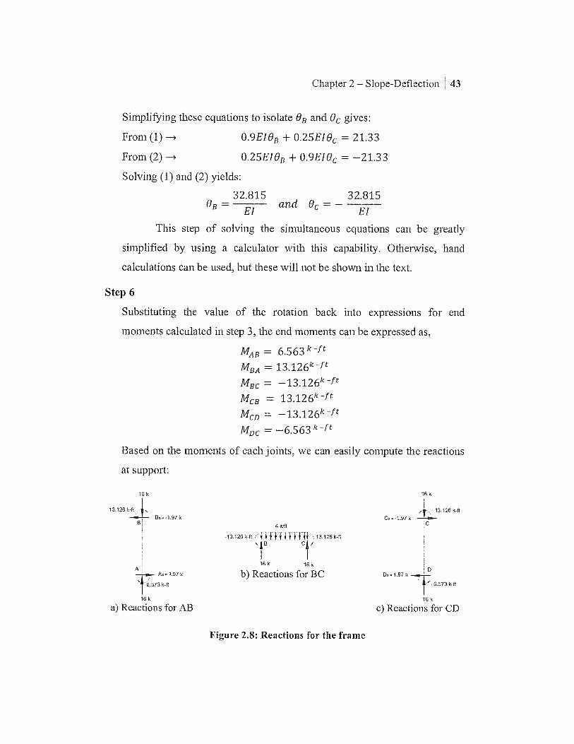
Step 6
Substituting the value of the rotation back into expressions for end
moments calculated in step 3, the end moments can be expressed as,
MAB = 6.563 k - f t
MBA = 13.126kt- f t
MBC = —13.126k -f t
MCB = 13.126k -ft
MCD = —13.126k -ft
MDC = —6.563 k - f t
Based on the moments of each joints, we can easily compute the reactions
at support:
16k
16 k
Figure 2.8: Reactions for the frame

44 Chapter 2 - Slope-Deflection
Alternatively, the relative stiffness factors could have been used to
solve this problem. If one were to use this concept, the relative stiffness
factors for AB and BC would be as follows: 2* /
KAB—rei = — so (20) = 4
2*I KBC—rel = 8 (20) = 5
Here, the relative stiffness factors (-2Z) have been multiplied by the
LCM (Least Common Multiple) to simplify the calculations. Also, E and I
are not included in the relative stiffness factors because they must be
constant in all members to use Krei . The rotations obtained using this
concept are different than those found using the actual stiffness factors
because they are modified according to the LCM. The point to be noted is
that, the final end moments remain the same and calculation is facilitated.
If one was to use these relative stiffness factors and modified slope-
deflection equations, 2.2a and 2.2b, the value of OB comes out to be
1.6408. However, the actual end moments remain the same.
El El 32.815 ME = OB * — 6.563k-ft A El
MAB—rei = 4[0B] = 4 * 1.6408 = 6.563k-ft

MAB A
F1
Ls* MBA B (---- HB
b) Column AB
HD
MDC D< HD
c) Column CD
w
UlUU U141,1 ,1,
Yi
F1
B
1 VD
h2
VD
A
Chapter 2 — Slope-Deflection 45
2.6 Derivation of Shear Condition for Frames (With Joint Movement)
When analyzing frames with joint movement, an extra unknown (A or
`11) is added to the usual unknown displacements. This means an extra equation
is needed. The equation is obtained from what is known as the "shear
condition" at the base supports of the frame.
a) Frame with side sway
Figure 2.9: Frame with sidesway — Basic concept illustration
For a typical frame (Fig. 2.9), the shear condition obtained from the
basic equation IF, = 0 is given as,
Fl — HB — HD = 0 (2.13)
Where HB and HD can be found by taking E MA = 0 and E Mc = 0 using
Figures 2.9b and 2.9c.

46 I Chapter 2 — Slope-Deflection
This would yield the flowing two equations.
HB MAB+MBA
hi (2.13a)
CD+MDC HD =
(2.13b) 2 11 Equations 2.13a and 2.13b are written with the assumption that the end
moments of a column are clockwise (positive). Figure 2.9b and 2.9c show the
free body diagrams for columns AB and CD with which the expression for HB
and HD are derived. Equation 2.13 has to be solved in addition to the other
joint equilibrium equations.
The rest of the procedure remains same as outlined in Sec. 2.3.
2.7 Application of the Slope-Deflection Method to Analysis of Frames With Joint Movement
An example is solved below to illustrate the analysis of a frame with sidesway
using the slope-deflection method.
Example 2.7.1
Determine the reactions at the supports of the frame shown in Fig. 2.10. A = 100 in2, E = 29000 ksi and I = 833 in4.
4 k/ft
8 ft
1 0 ft
Figure 2.10: Indeterminate Frame (sidesway)

4 k/ft
8 ft
10ft
A Figure 2.11: Bending of frame in Ex. 2.7.1
Chapter 2 — Slope-Deflection 47
Solution
Step 1
The fixed-end moments are calculated using Table 1A found in the
appendix.
4*8 2 MFAB = 12 = _2133k-f t
4*82 MFBA 12
2133k-f t
Step 2
The unknown displacements are Om Oc and WBc. KI = 3
Step 3
The slope-deflection equations for this structure can be written as,
MAB = 2E18- [2(0) + OB ] — 21.33 = •T:OB —21.33 (1)
(Note: OA = 0 due to fixed support at A)
MBA = 2E1.8- [20B + 0] + 21.33 = 512 OB + 21.33 (2)
MBC = 2E7-1-6[20B + 9C — 'BC] 1 3) (
McB = 2E3/-0- [20c + OB — tif BC] 4) (

48 I Chapter 2 - Slope-Deflection
Step 4
Moment equilibrium required: MBA + MBC
(5) Roller support at C ---> MCB 0
(6)
Due to symmetrical loading there is no moment in member BC, but the
structure will still sidesway. Hence,
MBC 0 (7) Step 5
From Equations (5) and (7) ---> MBA °
Substitute in (2) -->
2OB + 21.33 = -> OB =
Step 6
Substituting the value of the rotation back into expressions for end
moments calculated in step 3, the end moments can be expressed as,
MAB = -32k-ft
Step 7 and Step 8
The reactions at A (A, and Ay) and C (Cy) are calculated from principles of
statics:
-4 ET, = 0 --> A x = 0
EWA = 0:
-32+32 * 4- Cy * 8 = 0 -> C = 12k (T)
+TET"), = 0:
Ay + 12 - 32 = 0 -) Ay = 20k (T)
42.66 El
After the reactions are obtained, the Bending Moment Diagram (BMD) and the
Shear Force Diagram (SFD) can be drawn as needed.

Chapter 2 — Slope-Deflection 49
2.8 Summary
In this chapter, the fundamentals of a classical method, called the slope-
deflection method, were discussed. This was followed by examples applying it
to beams and frames. The slope-deflection method essentially consists of
solving a set of simultaneous equations where the unknown values are
displacements. Finally, end moments are calculated using these displacements.
This method is easy to use; and unlike the force method, does not require
knowing how to do deflection calculations.

50 Chapter 2 — Slope-Deflection
Problems
Analyze Problems 2.1 to 2.3 using the slope-deflection method.
Problem 2.1 Determine the reactions at the supports of the beam shown in
this figure. El is constant.
1.5 k/ft
A
C
10 ft
12 ft
Problem 2.1
Problem 2.2 Determine the reactions at the supports of the frame shown in
this figure. A = 100 in2, E = 29000 ksi and I = 833 in4.
.4, 32k
8 ft
10 ft
Problem 2.2

Chapter 2 — Slope-Deflection 51
Problem 2.3 Determine the reactions at the supports of the frame shown in
this figure. A = 100 in2, E = 29000 ksi and I = 833 in4
32 k
Br
2ft
*NO
8ft
Problem 2.3 2.3
c
loft


Chapter
Displacement Method of Analysis: Moment Distribution Method
3.1 Basic Concepts of Moment Distribution Method
Hardy Cross originally developed the moment distribution method in
1930. It is a classical and iterative method. It essentially consists of locking
and unlocking each joint consistent with the actual boundary conditions. This
means the whole procedure of moment distribution is carried out in such a way
that at the end of it, the final end moments for a hinge (pin) joint should be
zero while a fixed joint can have any amount of moment. Analysis of a
structure essentially involves finding the end moments for each member. It will
be interesting to compare the moment distribution method with another
classical method — the slope-deflection method (discussed in Ch. 2). In the case
of the slope-deflection method, finding end moments of members is a two-step
process. The first step is finding the slopes at each joint and the second is
finding end moments for each member. On the other hand, the moment
distribution method directly gives the end moments for each member. The
moment distribution method, like the slope-deflection method, uses fixed-end
moments and stiffness factors. Additionally, the moment distribution method
uses distribution factors. It is through the distribution factors that the moment
distribution is essentially carried out because they dictate how much moment a
specific joint will transfer. Distribution factors are obtained using the stiffness
factors for each member in such a way that it reflects the property of the joint.
Thus, since the total moment at a hinge joint is zero, the distribution factor at a
hinge joint is one. Similarly, the distribution factor at a fixed joint is zero as

54 I Chapter 3 — Moment Distribution
the fixed joint can carry any amount of moment. The distribution factor will be
discussed with more detail in section 3.2.3.
3.2 Stiffness Factor, Carry-Over Factor and Distribution Factor
Three important factors used in the moment distribution method are the
stiffness factor (K), Carry-Over factor (CO) and the Distribution Factor (DF).
These will be described in the following sections.
3.2.1 Stiffness Factor
L
Figure 3.1: Beam with moment applied at B
Fig. 3.1 shows a beam with a moment applied at B. It can be proven that,
Or,
Where,
4E1 MBA = L u
oi B
MBA = KOB
K= 4E1 L
(3.1)
(3.2)
(3.3)
In Eq. 3.3, K is the stiffness factor for member AB, which is defined as
the amount of moment needed at B to induce a unit rotation (BB = 1 rad).
Other books sometimes modify the stiffness factors based on support
conditions, but in this book the authors will advocate using the stiffness factor
K = 4EI/L for all members. Using K = 4E1 /L for all members will simplify
the analysis and provide the same answers.

Chapter 3 — Moment Distribution = 55
3.2.2 Carry-Over Factor (CO)
In Fig 3.1, it can be proven that the moment induced at A is,
2E1 al MAB L uB (3.4)
From Eq. 3.1 and Eq. 3.4 it can be seen that the carry-over moment,
moment induced at A, is 1/2 of the applied moment at B. This implies that the
carry-over factor, which is the ratio of MA to MB, is 0.5. Thus it can be stated
that for a beam simply supported at one end and fixed at the other, the CO is
0.5. This concept will be applied in the moment distribution procedure.
3.2.3 Distribution Factor (DF)
(DF)lnember Kmeniber
nmember (3.5)
Where, Km ember includes all members connected to the joint considered.
A
a) b)
Figure 3.2: Concept of distribution factors

56 I Chapter 3 — Moment Distribution
Using Fig. 3.2a, the distribution factors can be defined as,
(DF)AB = KAB I (KAB KAC KAD KAE) (3.5a)
(DF)AC = KAC I (KAB KAC KAD KAE) (3.5b)
(DF)AD = KAD l(KAB KAC KAD KAE) (3.5c)
(DF)AE = KAE I (KAB KAC KAD KAE) (3.5d)
The distribution factor at a fixed support is zero because it "absorbs"
moments rather than distributing them. Applying Eq. 3.5 at joint E proves this
as can be seen below:
DFEA KEA 0
KEA+ °° (Fixed support)
In theory, a fixed support is "infinitely" stiff because it could take a
moment of any size. This makes the denominator of the above equation co,
therefore DF = 0 for all fixed supports. Similarly, DF = 1 for pin and roller
support at the end of a beam. Considering joint C in Fig. 3.2b, the distribution
factor would be calculated as follows:
KCA DFcA 1 KCA
(End-pin support)
Here, you can see that since there is only one member attached to end
joint C, the stiffness factor is 1. This is true for all pin and roller supports at the
ends of continuous beams.

Chapter 3 – Moment Distribution 57
3.3 Analysis of Continuous Beams by Moment Distribution Method
The basic procedure for solving problems containing continuous beams
using the moment distribution methods will be explained first followed by an
example.
3.3.1 Basic Procedure for Moment Distribution
The general procedure for analysis of beams and frames is the same.
Therefore, the procedure listed below is applicable to beams and frames (i.e.
structures essentially in flexure or bending):
1. Calculate the stiffness factors (K) for each span using the following
equation: 4E1 K = — (3.3)
2. Calculate the Distribution Factor (DF) for each member using the
following relation: K member
DFmember Kmember
Where, E Kmember includes all members connected to the joint considered.
Note:
Distribution factors that are unknown must be solved using
Equation 3.5, but those that are known, fixed supports and end-
pin supports, can be found immediately.
3. Calculate the fixed-end moments using Table lA in the Appendix. This
step means locking all the joints. The sign convention used is: clockwise
moments and rotations are considered positive.
4. Set up the moment distribution table by entering the calculated fixed-end
moments for each member and the distribution factors for each joint. The
(3.5)

58 Chapter 3 — Moment Distribution
table will need to include all the members, and will look similar to the
following depending on the amount of joints:
Joint Member DF
A AB
B BA BC CB
C CD
D DC
MF Bal CO Bal
i 1 1 1 1 I I
Final
5. Start the 1st cycle of moment distribution by unlocking each joint. Sum
up the MF for all members connected at each joint to get the unbalanced
moment (M .--(unbalanced))• Multiply this moment by the respected DF and
invert the sign to get the Bal for that member. The following relationship
can be utilized:
B al Al(unb alanced) * DF
At a pin support, when summing the MF and Bal of each cycle, both
members will be delivering the same moment with opposite direction
(sign) to the joint. This means the joint is balanced. Fixed supports will
have a residual moment.
6. Find the CO by carrying Bal values across members (from joint to joint)
with a factor of 1/ 2. Then get the new unbalancing moments by using the
CO. Step 5 and 6 involve locking and unlocking the joints. The first
locking moments are due to fixed moments (caused by the given loads).
The successive locking moments are obtained through CO.
7. Continue the balancing until the final unbalance at each joint is about I%
of the initial unbalance moment at any joint.

Chapter 3 - Moment Distribution : 59
3.3.2 Example for a Continuous Beam
The procedure discussed above will now be applied to a multi-span continuous
beam.
Example 3.3.2.1:
Analyze the continuous beam shown in Fig. 3.3 using the moment distribution method.
36 k
C
10ft
12ft
Figure 3.3: Continuous beam
Solution
Step 1
Stiffness Factors are not needed here because all the distribution factors are
known.
Step 2
DFAB = 0 (Fixed support)
DFBA = 1 (End-pin support)
DFBc = 0 (No moment is transferred from B to C)
Step 3
MFAB = MFBA - MFBC 36 * 12 = -432 k- f t
Note: MFBc is negative because the internal moment caused by the loading,
acts in the counterclockwise direction (opposite to the external moment
at that point).
A B

60 Chapter 3 — Moment Distribution
Step 4 — 7
The moment distribution table is set up as shown in Table 3.1. First,
the joints A and B are added to the table along with the corresponding
members. Joint C is not part of the table because there is no support. Then,
the distribution factors of each member are added based on their support
type, and whether they are intermediate or end supports. In this case, joints
A and B are end supports because the cantilever portion can be simplified
into a moment acting at the BC location. Members AB and BA have no
fixed-end moments because there is no loading on the span of the member.
The balance for the first cycle in member BA needs to be 432 to satisfy
joint equilibrium at joint B. This number can be found either by inspection
(-432 + x = 0) or by the standard procedure of:
Bal = — M(unbalanced) * DF
BalBA = —(MBc. + MBA) *1
BalBA = — (-432) * 1 = 432f t k
The carry over only occurs from joint B to A because moments are
not carried to C (cantilever), or from joint A because it is fixed (DF = 0).
In this problem, the process is repeated only one more time because the Bal
in the second iteration was all zero. Other problems will require more
iteration so that the Bal is 1% of the initial unbalanced moment.
Table 3.1: Moment distribution table Joint
Member A
AB BA
B
BC
DF 0 1 0
MF 0 0 -432
Bal 0 432 0
CO ..<
216 0 0 Bal 0 0 0
Final 216 432 -432

Chapter 3 - Moment Distribution 61
The answers found here, M -AB = 216ft-k- MBA = 432f t-k
and MBC = -432f t-k (.5 are the same as found by the force method in
Chapter 1 (Ex. 1.5.2.1) and by the slope-deflection method in Chapter 2
(Ex. 2.3.1), but with less work. This is a good example of how powerful
the moment distribution method is; yet the true power of this method will
be seen once more complicated examples are solved.
3.4 Analysis of a Continuous Beam with Support Settlement by Moment Distribution Method
The procedure for moment distribution discussed in Sec. 3.1 is now
applied to a continuous beam with support settlements and no other load. The
fixed-end moments at each end are obtained using Equation 3.6a or 3.6b.
A
(3.6a)
MFBA
Figure 3.4: Effect of displacement at B
From the right column of Table 1A, when considering the far end piimed then,
-3E1A MFAB = L2
From Table 1A, when considering both ends fixed then,
-6EIA MFAB = MFBA = L2 (3.6b)
When solving problems where the far end is pinned, it is possible to
take advantage of the right column of Table 1A, which gives fixed-end
moments for a structure where the far end is pinned. An example of a far end
pinned member is member AB. Although this method can reduce the number

62 I Chapter 3 — Moment Distribution
of calculations in the moment distribution table, it is not the only way to solve
the problem. Alternatively, the standard fixed-end moments can be used for all
joints, no matter the given support condition (fixed, pin, or roller). The
difference between the two methods is that assuming all joints are fixed (using
the left side of Table 1A) can be easier to set up, but it will often involve more
iteration in the moment distribution table. In the next example both methods
will be used to show that both methods provide the same answer without a
great deal of difference in procedure.
Example 3.4.1:
Determine the reactions at the supports of the beam shown in Fig. 3.5 by the moment distribution method. Take E = 29,000 ksi and I = 446 in4. The su s port at B is displaced downward 1 in.
A
10 ft 12 ft
Figure 3.5: Statically indeterminate beam with support settlement
Solution
Method 1
Step 1
Stiffness Factors are not needed here because the distribution factors are
known.
Step 2
D FA B (Fixed support)
D FB A 1
(End-pin support)
DFBc = (No moment is transferred from B to C)
Chapter 3 — Moment Distribution j 63
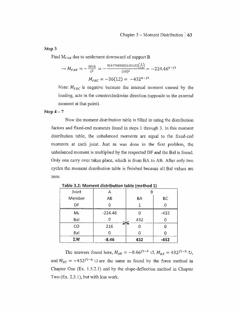
Step 3
Find MFAB due to settlement downward of support B
3E/A 3(4176000(0.0215)N MFAB 12 —224.46k-ft L2 (102
MFBC = —36(12) = — 432k-f t
Note: MFBC is negative because the internal moment caused by the
loading, acts in the counterclockwise direction (opposite to the external
moment at that point).
Step 4 — 7
Now the moment distribution table is filled in using the distribution
factors and fixed-end moments found in steps 1 through 3. In this moment
distribution table, the unbalanced moments are equal to the fixed-end
moments at each joint. Just as was done in the first problem, the
unbalanced moment is multiplied by the respected DF and the Bal is found.
Only one carry over takes place, which is from BA to AB. After only two
cycles the moment distribution table is finished because all Bal values are
zero.
Table 3.2: Moment distribution table (method 1) Joint
Member
A
AB
B
BA BC
DF 0 1 0
MF -224.46 0 -432
Bal 0 432 0
CO 216 0 0 Bal 0 0 0
EM -8.46 432 -432
The answers found here, MAB = —8.46ft-k MBA = 432ft-k
and MBC = —432f t-k 0 are the same as found by the force method in
Chapter One (Ex. 1.5.2.1) and by the slope-deflection method in Chapter
Two (Ex. 2.3.1), but with less work.

64 Chapter 3 - Moment Distribution
Method 2
Step 1
Stiffness Factors are not needed because the distribution factors are known.
Step 2
DFAB 0 (Fixed support)
DFBA - 1 (End-pin support)
DFBC = 0
(No moment is transferred from B to C)
Step 3
MFAB = MFBA
Step 4
6EIA 6(4176000)(0.0215)(1 - 12) = 488.92k-f t L2 (10)2
Since the left column fixed-end moments are used, member BA
now has the same moment as member AB. The unbalanced moment for
joint B is found by summing up MFBA and MFBC. This value is then
multiplied by the distribution factor of members BA and BC as seen below:
Bal = --M(unbalanced) * DF
BaIBA = -(MBC + MBA) * 1
BalBA = -(-432 + (-448.92) ) * 1 = 880.92ft-k
Next, the carry-over factor (1/2) is applied from joint B to Joint A,
as indicated by the arrows. From here all balances are zero so the moments
are summed up and the table is complete.
Table 3.3: Moment distribution table (method 2) Joint
Member DF
A AB 0
BA 1
B BC 0
MF -448.92 -448.92 -432
Bal 0 880.92 0 .><
CO 440.46 0 0 Bal 0 0 0
EM -8.46 432 -432

Chapter 3 — Moment Distribution 65
When comparing the two methods, the final moments are exactly the
same, and found in only two cycles. This proves that both methods can be used
for a given problem based on preference. The authors of this book prefer
method 2 due to the simplicity of finding the fixed-end moments. It should also
be noted that the results are identical to those obtained using the slope-
deflection method in Ex. 2.4.1 which can be seen in the chapter summary in
Section 3.7.
3.5 Application of Moment Distribution to Analysis of Frames Without Sidesway
The analysis of frames without sidesway is similar to that of continuous
beams. The procedure described in Sec. 3.3 will be used to analyze frames
without side sway. An example is discussed below to illustrate this concept.
Example 3.5.1:
Determine the moments at each joint of the frame shown in Fig. 3.6 by the moment distribution method. E = 29,000 ksi, A = 16 in2 and I = 446 in4 for all members.
4 k/ft
10 ft
8 ft
Figure 3.6: Indeterminate frame (no sidesway)

66 Chapter 3 - Moment Distribution
Solution
Step 1 4E1 4E1 4E1
KAB = KBC = and = 10 8 10
Step 2
In this problem we must find the distribution factors for the members at
joints B and C using Equation 3.5 because they are unknown. At joint B, 4E1
0 DFBA = 4E11 4E1 = 0.444
10 8
-> DFBC = 1- 0.444 = 0.556
Similarly at joint C, 4E1
- 8 -> DF CB — 4E1 4E1 = 0.556 10 8
-4 DFcD = 1- 0.556 = 0.444
Step 3
The fixed-end moments are found using Table 1A.
wg = 12
4(8)2 MFBC
21.33k-ft 12
4(8)2 21.33k-f t MFCB 12
Step 4-7
All the joints, members, distribution factors, and fixed-end
moments are filled in based on steps 1 - 3. A sample calculation for the
balance of the first cycle for members BA and BC is given below:
Bal = -M(unbalanced) * DF
BalBA — (MBC+ MBA) * 0.444
BalBA = -(-21.33 + 0) * 0.444 = 9.48f t-k
Ba1BC = -(M.Bc + MBA) * 0.556
Ba/Bc = -(-21.33 + 0) * 0.556 = 11.85f t-k

Chapter 3 - Moment Distribution I 67
Carly-over is applied between joints B and C, from B to A, and
from C to D. This process is repeated until the balance is about 1% of the
original unbalanced moment. Lastly, values for the internal end moments
of each member are found by summing up all the entries in each members
column starting with the fixed-end moment.
Table 3.4: Moment distribution table Joint
Member
DF
A
AB
0
BA
0.444
B
BC CB
0.556 0.556
C
CD
0.444
D
DC
0
M F 0 0 -21.33 21.33 0 0
Bal 0 9.48 11.85 -11.85 -9.48 0 CO 4.74 0 -5.925 5.925 0 -4.74 Bal 0 2.633 3.292 -3.292 -2.633 0
CO 1.317 0 -1.646 1.646 0 -1.317 Bal 0 0.731 0.914 -0.914 -0.731 0 CO 0.366 0 -0.457 0.457 0 -0.366 Bal 0 0. 203 0.254 -0.254 -0.203 0 CO 0.102
><. 0 -0.127 0.127 0 -0.102
Bal 0 0.056 0.071 -0. 071 -0.056,, 0
CO 0.028 ?‹.
0 -0.0361..?‹
0.036 deA
0 -0.028 Bal 0 0.016 0.02 -0.02 -0.016 0 EM 6.55 13.12 -13.12 13.12 -13.12 -6.55
The answers for the reactions at the base would be the moments,
MAB 6.55k-f t Z..) and MDC = -6.55k-f t 0 . These values of end
moments are very similar to the results of slope-deflection method.
Note: MAB is the internal moment at joint A in member AB and is also
the reaction at the support, MA. MA has the same magnitude and
direction as MAB
The vertical reactions at the base can be found using basic statics
because the loading is symmetrical (half of the total distributed load force

68 Chapter 3 — Moment Distribution
applied to each support acting upward). Also the horizontal forces at the
base can be found in the following fashion:
13.12k- f B
B
6.55k-f t A
Figure 3.6.1: Member AB
= 0 :
13.12 + 6.55 — 10A, = 0 A, = 1.97 k -+
For the whole frame:
= 0 : A, + = 0 D„ = —A„ = —1.97 k
-I-
10 ft
A,
3.6 Application of Moment Distribution to Analysis of Frames with Sidesway
In this section, the basic concept involved in analysis of a frame with
sidesway by moment distribution will be discussed followed by an example.
3.6.1 Basic Concepts: Application of Moment Distribution to Analysis of Frames with Sidesway
To solve a frame with side sway, the principle of superposition will be
utilized, Fig. 3.7. This analysis involves two steps: 1) Analyze the frame with
sidesway being restrained and with the applied loading, see Fig. 3.7b and 2)
Analyze the frame with only sidesway and no applied loads, Fig. 3.7c. In both
steps the moment distribution table will need to be used.

Chapter 3 — Moment Distribution 69 F2 F3
MDC
VD
a) Given frame showing sidesway
b) Sidesway restrained c) Sidesway allowed
Figure 3.7: Principle of superposition applied to a frame with sidesway
The basic superposition equation for the moment at can be derived as,
MNF NF kW ! NF (3.7)
Where,
k = R/R'
(3.8)
N = Near joint of a member
M = Far joint of a member

70 I Chapter 3 — Moment Distribution
The single prime denotes the moments on the restrained frame, Fig.
3.7b, and the double prime denotes the moments due to sidesway only, Fig.
3.7c. The expressions for sidesway moments are given in Eq. 3.6a and 3.6b.
The solution of frames with sidesway using the moment distribution
methods essentially involves solving two moment distribution tables. The first
table is for the frame restrained against sidesway having the given loading, and
the second table is for the frame with sidesway only and no applied loads. The
last portion of the superposition is relating the two sets of results through the k
factor, Eq. 3.8. The process of filling in the moment distribution table will not
change for frames with sidesway.
3.6.2 Example of Moment Distribution: Analysis of Frames with Sidesway
An example in which a frame with sidesway, or joint translation, is
solved using the moment distribution method will be discussed below in
Example 3.6.2.1

Chapter 3 — Moment Distribution 71
Example 3.6.2.1:
Analyze the frame shown in Fig. 3.8 using the moment distribution method. Determine the reactions at the supports of the frame shown in this figure. A =100 in2, E = 29000 ksi and I = 833 in4.
II l 114
1k/ft
llllllllllll
:A
8ft
10ft
Figure 3.8: Frame with sidesway
Solution
Step 1
Here we need to calculate the stiffness factors of the members connected to
joint B, because we do not know DFBA or DFBC. 4E1
Step 2
KAB = KBA
KBC = KCB
8 =0.5E1
— 4E1 10 = 0.4E1
—
The distribution factors for members BA and BC are calculated
below. DFBc is found by 1 — DFBA because the sum of the distribution
factors at joint B must be 1. Also, since C is an end-pin support, DFCB 0.5EI
DFBA = = 0.556 0.5E1 + 0.4E1
DFBc =1 — 0.556 = 0.444
DFCB = 1 (end-pin support)
is 1.

72 Chapter 3 - Moment Distribution
Step 3 - Restrained frame
The restrained frame includes an artificial support to inhibit
sidesway at joint C. R is the reaction force at the artificial joint, C, due to
the given loading. This is the first part of the principle of superposition
applied to the frame.
R
Figure 3.8: Restrained frame (no sidesway)
The fixed-end moments for member AB are calculated using Table
lA and are shown below. There are no fixed-end moments on member BC
because there is no external loading on the member's span. 4.82 4.82 = -2 1.3 3R-f t and MFBA = 21.33k- f t 12 12
Step 4
Table 3.5, the moment distribution table for the restrained frame, is
set up using the distribution factors and the fixed-end moments found in
the first three steps. Then, iteration of Bal and CO are carried out, making
sure that joint equilibrium is satisfied in each cycle. The carry-over factor
of 1/2 is applied between joints where possible. Summing up each column
yields the moments at each end of the members.
MFAB

= 0 • B • -8.008 + 10C, = 0 C„ = R = 0.8008 k
Chapter 3 - Moment Distribution 73
Table 3.5: Moment distribution table for the restrained frame
Joint
Member
DF
A
AB
0
B
BA
0.556
BC
0.444
C
CB
1
MF -21.33 21.33 0 0
Bal 0 -11.859 -9.471 0 CO -5.930 0
1?‹. 0 -4.736
Bal 0 0 0 4.736 CO 0 0 2.368 0 Bal 0 -1.316 -1.051 0 CO -0.658 0 0 -0.526 Bal 0 0 0 0.526 CO 0 0 0.263 0 Bal 0 -0.146 -0.117 0
Final -27.918 8.008 -8.008 0
The results obtained here are, M'AB = -27.918k-ft (.5,
M I BA = 8.008k- f t J, and M'BC = -8.008k-f t (5.
Calculate R:
Using the internal moments found for the restrained frame in Table
3.5, we can now find the force R.
8.008k-f t
0.8008 k
10 ft
4--- 0.8008 k
Figure 3.9: Calculation of R using member BC

10 ft
74 Chapter 3 - Moment Distribution
Using Figure 3.9, the following calculation can be made:
8.008f t-k Required couple = =
10ft 0.8008 k
In order to satisfy equilibrium on this member, the couple must be acting in
the opposite direction as the MBC, therefore:
R = 0.8008 k
Note: R is positive because it is acting in the direction assumed, Fig. 3.8.
Frame with sidesway and artificial joint removed
Again, the fixed-end moments on the members need to be found.
Member BC will have a fixed-end moment due to deflection at C.
Typically this would involve using Table I A found in the appendix, but if
the columns have the same displacement (s'), E, I, and L, then an arbitrary
value can be used with the correct direction. In this problem there is only
one column and one moment so no problems will be encountered using an
arbitrary moment of 100k-f t applied clockwise at B.
..\100 k- f t
8 ft
Figure 3.10: Frame with sidesway and artificial joint removed
To set up Table 3.6, all we need are the distribution factors and the
single MF for member BC. Then, the typical procedure of Bal and CO are
used to fill in the rest of the table and find the end moments at each
member.
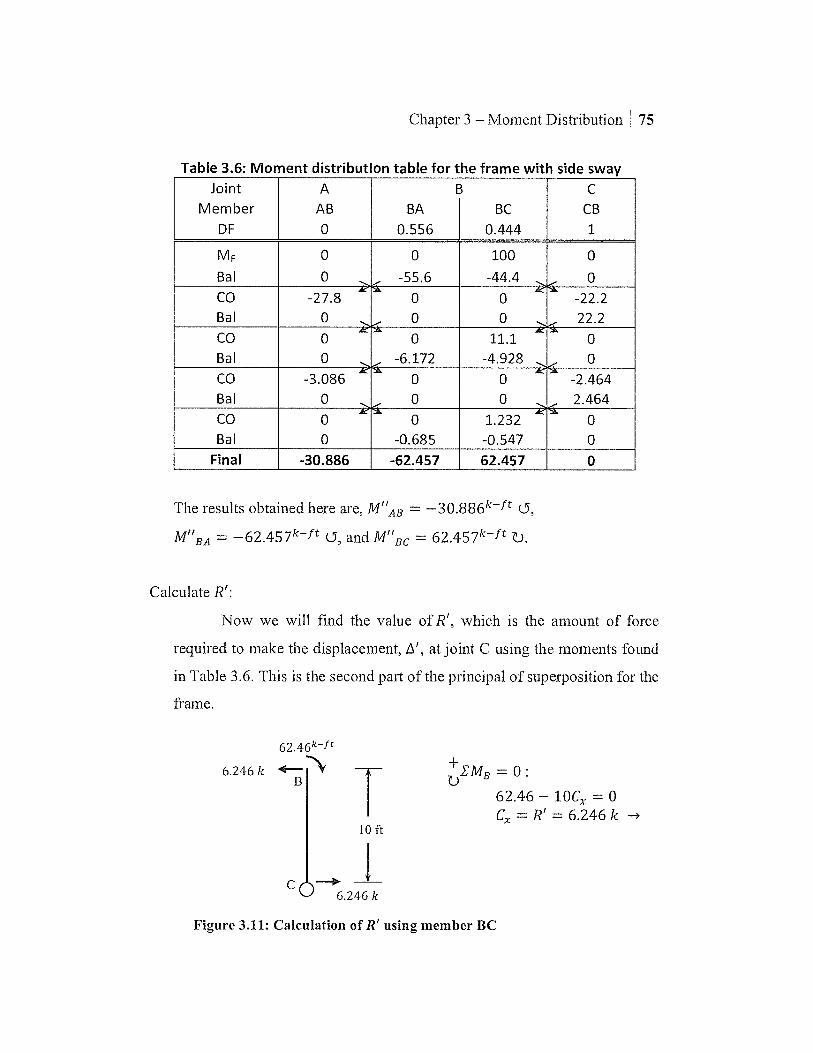
62.46k-f t 6.246 k 4-
B
10 ft
6.246 k
Chapter 3 - Moment Distribution 75
Table 3.6: Moment distribution table for the frame with side sway Joint
Member OF
A AB 0
B BA
0.556 BC
0.444
C CB 1
MF 0 0 100 0 Bal 0 -55.6 -44.4 0 CO -27.8 0 0 -22.2 Bal 0
2 0 0 22.2
CO 0 0 11.1 0 Bal 0 -6.172 -4.928 0 CO -3.086 0 0 -2.464 Bal 0 0 0 2.464 CO 0 0 1.232 0 Bal 0 -0.685 -0.547 0
Final -30.886 -62.457 62.457 0
The results obtained here are, M"AB = -30.886k- ft (-5,
M"BA = -62.457k- ft (5, and Mif Bc = 62.457k-ft Z.).
Calculate R':
Now we will find the value of R', which is the amount of force
required to make the displacement, at joint C using the moments found
in Table 3.6. This is the second part of the principal of superposition for the
frame.
EM = 0 B • 62.46 - 10C, = 0 C, = = 6.246 k
Figure 3.11: Calculation of R' using member BC
76 Chapter 3 — Moment Distribution
Using the figure above, the following calculation can be made:
62.46f t—ic Required couple =
10ft = 6.246 k
In order to satisfy equilibrium on this member, the couple must be acting in
the opposite direction as the MBC, therefore:
R' = 6.246 k
Note: R' is positive because it acts in the direction assumed in Fig. 3.10
Final moments:
Using the ratio of R/R, we can complete the superposition and find
the amount of moment that needs to be added or subtracted from the
original moments found for the restrained frame.
R MAB = Mi AB (restrained) + R, M AB(sidesway)
0.8008 —27.918 + 30.886) = —32k-ft MAB 6.246 (
0.8008 MBA (
= 8.008 + 62.46) = Ok-f t 6.246 0.8008
= —8.008 + (62.46) = Ok-f MBC t 6.246

Chapter 3 — Moment Distribution 77
The reactions at A (Ax and Ay), at C (Cy) are calculated from principles of
statics:
F =O— A= 0 +EMA = 0 : —32 + 32 * 4 — Cy * 8 = 0
Cy = 12k(T)
+I .EFy = 0: Ay + 12 — 32 = 0
Ay = 20 k (T)
4k/ft
32 k-fLA
20 k
12 k
Figure 3.12: Final reactions for the frame

78 Chapter 3 - Moment Distribution
3.7 Summary
A concise description of the concept of the moment distribution is
presented in this chapter. This is followed by few problems dealing with
continuous beams, frame without joint movements (sidesway) and with joint
movements. It should be noted that moment distribution method directly gives
moments.
Table 3.7 shows a summary of the solutions to example problems from
Chapter 1 to 3. The answers for each method are very close if not exactly the
same, showing that any method may be used to analyze an indeterminate
structure. The moment distribution method was the only method that showed
slight differences. These can usually be minimized with more iteration.
Table 3.7: Comparison of example problem solutions from Ch. 1- 3
Chapter 1
(Force Method)
Chapter 2
(Slope-Deflection)
Chapter 3
(Moment
Distribution)
Beam BY ' =100 8k T
A = -64.8 k I Y ' MA = 216k-ft Z.)
By = 100.8 k T
A = -64.8k I Y MAR = 216k- f t Z)
By = 100.8 k T
AY = -64.8 k I
MAR = 216k-f t Z.)
Beam With
Settlement
B = 78 356 k T By • AY = -43.356 k I
MAB = 8.44k-f t 0
B = 78 354 k T y • AY = -43.354 k I
MAR = 8.46k- f t (.5
Frame No
sidesway
MAB = 6.573k-f t Z.)
MAR = 6.573k-f t (5 Ay = Dy = 16 k T
MAR = 6.55k-f t Z.)
MAB = 6.55k- f t (.5
Ay = Dy = 16 k T
Frame
With
Sidesway
A = 20 k T Y C = 12 k I y
MA = 32k-f t 0
A = 20 k T Y CY = 12 k I
MAB = 32k- f t 0
AY = 20 k T
C3, = 12 k I
MAR = 32k- f t 0

Chapter 3 — Moment Distribution ! 79
Problems
Analyze Problems 3.1 to 3.3 using the moment distribution method.
Problem 3.1 Solve Problem 2.1 by using the moment distribution method
Problem 2.1 repeated Determine the reactions at the supports of the beam
shown in this figure. El is constant.
1.5 k/ft
A
10ft 12ft .11*/10
Problem 3.1
Problem 3.2 Solve Problem 2.2 by using the moment distribution method
Problem 2.2 repeated Determine the reactions at the supports of the frame
shown in this figure. A = 100 in2, E = 29000 ksi and I = 833 in4.
32k
A B 8 ft
10 ft
Problem 3.2

_ - 2 ft
10ft
80 Chapter 3 — Moment Distribution
Problem 3.3 Solve Problem 2.3 by using the moment distribution method
Problem 2.3 repeated Determine the reactions at the supports of the frame
shown in this figure. A = 100 in2, E = 29000 ksi and I = 833 in4
32 k
8ft
Problem 3.3

Chap er
Direct Stiffness Method: Application to Beams
4.1 Basic Concepts of the Stiffness Method
The stiffness method is the most powerful method used for analysis of
structures. Almost all the computer codes written to analyze structures use the
stiffness method. One reason for the wide use is because the general procedure
of the stiffness method can be applied to any type of structure — beam, frame,
truss, or any structure for that matter. Also, it is very easy to use and can be
coded for analysis of entire structures.
4.2 Kinematic Indeterminacy
A structure's Kinematic Indeterminacy (KI) must be established before
solving a problem by the stiffness method. Again, Kinematic Indeterminacy is
defined as the total number of degrees of freedom for all the joints in a given
structure. Another method similar to the stiffness methods is the flexibility
method. The flexibility method is a matrix equivalent of the force method.
82 Chapter 4 — Direct Stiffness Method: Beams
4.3 Relation Between Stiffness Method and Direct Stiffness Method
While the stiffness method and the direct stiffness method are
essentially the same, well-known authors have drawn a distinction (Weaver
and Gere, 1990). Although the distinction is slight, it is important that this be
explained, especially for the undergraduate students in civil engineering for
whom this book is aimed at. In the stiffness method, the elements of a stiffness
matrix are derived from the basic principles of engineering mechanics
corresponding to the unknown displacements in the structure. In the case of the
direct stiffness matrix, the standard stiffness matrix for each element (whether
beam element, truss element or frame element) is used to assemble a structure
stiffness matrix. This matrix is then used to solve for displacements. Thus, the
direct stiffness method is more mechanical, to put it in plain tem.'s, and is very
easy to use. For this reason, the direct stiffness method is very popular and
widely used for analysis of any type of structure. The details of the direct
stiffness method will be discussed in the text and also applied to beam, frame
and truss structures with specific examples of each in this Chapter, Chapter 5,
and Chapter 6 respectively.
4.4 Derivation/Explanation of the Beam-Element Stiffness Matrix
A typical beam element, or member, is shown in Fig. 4.1. As can be
seen in Fig. 4.1, the action (A) and the displacement (D) are shown at the ends
of a typical beam element. {D) represents a generalized displacement
(translation or rotation) and {A} represents a generalized force (force or
moment). In the stiffness method, all loads will be distributed to the nodes. An
assembly of the various actions of a structure will constitute an action vector.
Similarly, an assembly of the various displacements of a structure will

Chapter 4 — Direct Stiffness Method: Beams 83
constitute a displacement vector. The reactions at the supports will also be
considered part of the generalized action vector. In Fig. 4.1, the actions and
displacements share a common number. To simplify things, one number and
symbol are often written to represent both entities (See Fig 4.3).
AI, DI A3, D3
Figure 4.1: Typical Beam Element
Note: The sign convention used in the stiffness method follows the right hand
rule. This means when curling the fingers on your right hand so that they
point in the direction of the moment or rotation, if your thumb points up, or
at you, then it is positive. Likewise, if it points down, or away from you,
then it is negative.
The basic definition of stiffness can easily be obtained from the
following equation which is the basic relationship used in the stiffness method,
(A) [K]{D} (4.1)
Where, {A} = Action vector
{D} = Displacement vector
[K] = Stiffness matrix
From Eq. 4.1, if {D} = 1 then [K] = {A}. This implies that the force
required to cause a unit displacement, is the stiffness. This is a very
important definition. This basic relation is used in the analysis of every
structure. If there is only one displacement, then [K] will be an element instead
of a matrix. [K] will be different from element to element when the length (L),
material (E), or cross section (I) are changed .

84 I Chapter 4 — Direct Stiffness Method: Beams
The matrix [K], used to relate the actions at joint A (near end) and joint
B (far end) to the displacements at joint A and B for a beam element, can be
expressed as (Weaver and Gere, 1990),
Di D2 D3 D4
12E1 6E1 12E1 6E1 Al
L3 L2 L3 L2
6E1 4E1 6E1 2E1 A2
L2 L L2 [K] = (4.2) 12E1 6E1 12E1 6E1
A3 L3 L2 L3 L2
6E1 2E1 6E1 4E1 A4
L2 L L2
Note: [K] is a symmetric matrix.
The action and displacement vectors for the beam element shown in
Fig. 4.1 can be expressed as,
Al
I
Di}
A-, D-)
(A} = A; and {D} = D3 ./../3
A4 D4
(4.3a & 4.3b)
The [K] matrix in Eq. 4.2 is written in structure coordinates (global x,
y, z axes), which is the same as member axes for a beam element. The member
axis changes with respect to the angle of the member. For example, the
member axis of a column (vertical member) would be rotated 90°
counterclockwise from the structure axis. Frame and truss elements that are not
horizontal will have different member and global axis. Hence, [K] can also be
called [Kmsi], which means stiffness matrix of the element in structure (global)
coordinates. It is to be noted that the way the stiffness matrix [K] is written in
Eq. 4.2 has to properly correspond with the action and displacement vectors in

Chapter 4 — Direct Stiffness Method: Beams 85
Eq. 4.3. As can be seen by the markings D1 through D4 in Eq. 4.2, the rows and
columns of [K] correspond to the translational and rotational displacements of
a given member. The pattern used in Eq. 4.2 is not arbitrary. The first row
corresponds to the translational displacement at the near (typically left) end of
the member and the second row corresponds to the rotational displacement at
the near end of the member. The third and fourth rows correspond to the
translation and rotation of the far (typically right) end of the member
respectively. This pattern must be followed for all members. Otherwise, the
[K] will be wrong and erroneous results will be obtained. The displacement
vector has to consist of translations and rotations at the near end followed by
translations and rotations at the far end. The same order is to be followed for
the corresponding actions when determining the action vector.
Another point to be noted is that some of the displacements in the
displacement vector will be unknown because they are free to displace. These
will be called {DA because they are the free displacements. On the other hand,
some displacements will be known because they are zero, or move a certain
amount (support settlement). These are designated as {DR } because they are the
restrained displacements. The free displacements are the ones to be obtained.
The actions corresponding to the free displacements are denoted {AF}. They
are known because they are the given applied loads. The unknown required
forces (such as reactions) are designated as {AR } because they correspond to
the restrained displacements.
To summarize, we want to find the unknown free displacements {DF }
and the unknown required forces {AR } using the known restrained
displacements {DR } and the known given loads {As).

86 Chapter 4 - Direct Stiffness Method: Beams
4.4.1 Global/Structure Stiffness Matrix
In addition to the element stiffness matrix [K], there is the structure
stiffness matrix [Ks], which links each individual member to the whole
structure. To make the member stiffness matrix for a given structure, the
following formula will need to be used:
Kjij ET KAi _ Di (4.4)
Where, n = Number of terms with the same i-j location.
KAi-D; = Value in the element stiffness matrix [K]
corresponding to Ai and D1
This formula is used to find each term of [K1] using the i-j location in the
element stiffness matrix.
4.5 Application of the Direct Stiffness Method to a Continuous
Beam
Here, the basic analysis procedure of the direct stiffness method for
continuous beams will be explained followed by an example.
4.5.1 Basic Procedure of the Direct Stiffness Method for Beams
1. Number the joints.
2. Number and define the members (with respect to how the member is
connected and to which joints). Follow the same order when defining
the displacements and the corresponding actions.
3. Determine KI (Kinematic Indeterminacy) and identify the unknown
displacements for the given structure. Then, number the displacements
starting from the free (unknown) displacements followed by the

Chapter 4 — Direct Stiffness Method: Beams i 87
restrained displacements. Within the free displacements any order can
be followed.
4. Write down the element stiffness matrix [K] from Eq. 4.2 connecting
the action vector and the displacement vector (from Eq.4.3) for all the
members in the given structure. Again, make sure that the translational
displacements are to be followed by rotational displacements (follow
the same corresponding order for action vector as well).
5. Assemble the structure stiffness matrix [K1] by combining the elements
of the same kind using the following equation.
Kfij (4.4)
Where, n = Number of terms with the same i-j location KA L —Di = Value in the element stiffness matrix [K]
corresponding to Ai and D.
KAL _ Di corresponds to all elements of the member stiffness matrix [K]
that relate to a specific action, Ai, and displacement, Di. The above
equation generates all the elements of the structure stiffness matrix [Ks ]
by combining all the elements corresponding to suffix i-j for all the
members.
If the numbering of the displacements is done starting from the free
displacements, the constitution of [K1], the joint structure stiffness
matrix, as it relates to structure action and displacement will be as
shown in Eq. 4.5 below.
{AF} — [ KFF KFR ] [DF1 (4.5)
AR KRR KRR DR
Where: KFF Portion of the structure stiffness matrix containing the known actions {AF } and the corresponding free displacements [M.
KFR = Portion of the structure stiffness matrix containing the known actions (AF) and the restrained displacements
88 Chapter 4 — Direct Stiffness Method: Beams
KRF = Portion of the structure stiffness matrix containing the unknown forces [AR ) and the free displacements {Dr).
KRR = Portion of the structure stiffness matrix containing the unknown forces {AR) and the restrained displacements (DR }.
6. The unknown displacements {DO can be obtained from the following
equation (which is derived from Eq.4.5),
(DA [KFF] l{AFN)
(4.6)
Where fil FN ) denotes the net actual and equivalent joint loads
corresponding to free displacements. Equivalent joint loads are member
loads that are distributed to the joints.
7. The unknown reactions {AR} can be obtained from the following
equation:
{AR} = [KRF]tDFI {ARO
(4.7)
Where {Am} denotes the net actual and equivalent joint loads
corresponding to restrained displacements. Using the above equation,
one can easily obtain (AR) knowing [K] and tD) obtained in previous
steps.
4.5.2 Example of a Continuous Beam Using the Stiffness Method
A continuous beam is solved below using the stiffness method described
above.

Chapter 4 — Direct Stiffness Method: Beams 89
Example 4.5.2.1
Determine the reactions at the supports of the beam shown in Fig. 4.2 using stiffness method. E = 29000 ksi, I = 446 in4.
36 k
10 ft
12 ft
Figure 4.2: Continuous Beam
Solution
Steps 1-3
Fig. 4.3 shows the beam after executing steps 1 through 3. Member
1 is defined as node number 1-2 and member 2 is defined as node number
2-3. This order needs to be used when writing the [K] matrix using the
action and displacement vector using Eq. 4.2 and Eq. 4.3 respectively. Note
that it could have been defined differently; like member 1 could have been
defined as 2-1.
The Kinematic Indeterminacy of this structure is 3 and the
unknown displacements are D1, D2 and D3 (translation at joint 1 and
rotations at joint 2 and 3). Figure 4.3 shows the displacement numbering is
done starting with the free displacements followed by the restrained
displacements. In this problem D1, D2 and D3 are free displacements
(unknowns) while D4 through D6 are the restrained displacements, which
are zero in this problem. As explained earlier, the actions {AF }
corresponding to {DF } are known (which can easily be obtained from the
fixed end moments). The {AR} corresponding to the known {DR} are the
unknowns.

90 I Chapter 4 — Direct Stiffness Method: Beams
D6 D2
D3 D1
1 2
Figure 4.3: Beam showing displacements
Step 4
The stiffness matrix [K1] for member 1 is obtained from Eq. 4.2 as
using the given properties of the beam element in the given problem.
Table 4.1: Stiffness matrix for member 1 5 4 6 3
89.82 5389.17 -89.82 5389.17 5389.17 431133.33 -5389.17 215566.67 -89.82 -5389.17 89.82 -5389.17
5389.17 215566.67 -5389.17 431133.33
The above matrix, [K1], relates the action vector (,45, A4, A6, A3}t to
the displacement vector {D5, D4, D6, D3}t . As pointed out earlier in the
basic procedure, displacements numbering follows the order of translation
followed by rotations. The same order is followed by the corresponding
actions as well. This is very important as noted earlier.
A derivation of some terms used in calculating the stiffness matrix
[K] is shown below.
K55 K66 = K65 = K56 = 12 El 12 (29000)(446)
= 89.82 L3 (10 * 12)
Similarly, other terms in the stiffness matrix [Ki] can be calculated.
In exactly same way, [K2], the stiffness matrix for member 2 can be
assembled using Eq. 4.2 and Eq. 4.3 as,

Chapter 4 - Direct Stiffness Method: Beams 91
Table 4.2: Stiffness matrix for member 2
[K2]
6 3 3742.48
359277.78 -3742.48
179638.89
2
-51.98 -3742.48
51.98 -3742.48
1 3742.48
179638.89 -3742.48
359277.78
51.98 3742.48 -51.98
3742.48
The above [K] matrix relates the action vector tA6, A3, A2, Ai}t to
the displacement vector tD6, D3, D2, DY. Again, translations are numbered
first followed by rotations.
Step 5
The structure stiffness matrix for this problem [K1] can be
assembled using Eq. 4.4 and the assembled matrices [K1] and [K2].
Table 4.2: Global/Structure stiffness matrix 1 2 3
359277.8 -3742.5 179638.9 -3742.5 51.98 -3742.5
179638.9 -3742.5 790411.1
0 0 215566.7 0 0 5389.2
3742.5 -51.98 -1646.7
4 5 6 0 0 3742.5 0 0 -51.98
215566.7 5389.17 -1646.7
431133.3 5389.17 -5389.2
5389.2 89.82 -89.82
-5389.2 -89.82 141.8
[Ki ]=
From the given condition, we can calculate,
0 4 CAEN) = 1-36 5
0 .16
From the above, the [KFF ] can be written as,
[KFF] 359277.8 -3742.5 179638.9 -3742.5 51.98 -3742.5 179638.9 -3742.5 790411.1

92 I Chapter 4 — Direct Stiffness Method: Beams
We can solve the displacement:
pp} = [KFF] * fAFN) - —0.04088 —4.50183 —0.01202
Calculate the reaction forces:
A 4 A5.[KRF],DF,_
—2592k—in —64.8 k
—216kl —64.8 k
A6 - 100.8 k - 100.8 k

Chapter 4 — Direct Stiffness Method: Beams ; 93
4.6 Summary
This chapter described the basic concepts of one of the most powerful
methods of structural analysis — the direct stiffness method. A general
procedure for solution of problems by the direct stiffness method is described
with application to continuous beams. The method, as described in this
chapter is general enough so that it can be applied to truss and frame as well.

94 Chapter 4 — Direct Stiffness Method: Beams
Problems
Analyze Problem 1.1 in Chapter 1 and Problem 2.1 Chapter 2 using the direct
stiffness method.
Problem 4.1 Solve Problem 1.1 using the direct stiffness method.
Problem 1.1 repeated Determine the reactions at the supports of the beam shown in this figure. Take EI constant.
20 kl
8m 4m
Problem 4.1
Problem 4.2 Solve Problem 2.1 using the direct stiffness method.
Problem 2.1 repeated Determine the reactions at the supports of the beam shown in this figure. EI is constant.
1.5 k/ft
A
10ft 12ft 1111■-■11
Problem 4.2

Chapter 5
Direct Stiffness Method: Application to Frames
5.1 Derivation/Explanation of the Stiffness Matrix for a Frame Element
The basic procedure of the direct stiffness method has been explained
in Chapter 4. The explanation is essentially a general procedure, which is also
applicable to frames. The only difference is that in the case of a frame, the
element stiffness matrix [K] for a frame element has to be used instead of for a
beam element. This is explained below.
Consider the general frame element shown in Fig. 5.1
A5, D5
A3, D3
Figure 5.1: Typical frame element with free and restrained supports

96 I Chapter 5 — Direct Stiffness Method: Frames
The member stiffness matrix for the frame element in structural
(global) coordinates, [Kmsi ] is given as,
Equation 5.1: Frame element stiffness matrix
1
AE
2
0
3
0
4
AE 0 0
L — L
0 12E1 6E1
0 12E1 6E1
L3 L2 L3 L2
0 6E1 4E1
0 6E1 2E1
L2 L L2 L
Ucsii= AE AE (5.1) 0 0 0 0 --
L L
12E1 6E1 12E1 6E1 0 0
L3 L2 L3 L2
0 6E1 2E1
0 6E1 4E1
L2 L L2
The global element stiffness matrix [Kmsi ] shown in Eq. 5.1 relates the
action vector f.A.1, A2, A3, A4, A5, A6}t to displacement vector
tD1, D2, D3, D4, D5, D6}t.
Again, like in the case of the beam, some of the elements of the
displacement vector will be zero. These will correspond to the restrained
displacement vector {DR }, which is subset of the {D} vector. Similarly, the
unknown, or free, displacements will be part of the free displacement vector
{DO, which is also a subset of the total displacement vector {D}.

Chapter 5 — Direct Stiffness Method: Frames 97
5.2 Application of the Direct Stiffness Method to a Frame
The process used to solve for the reactions of an indeterminate frame
using the direct stiffness method is explained below using Example 5.2.1.
Example 5.2.1
Determine the reactions at the supports of the frame shown in Fig. 5.2 using the direct stiffness method. A = 100 in2, E = 29000 ksi and I = 833 in4.
4llk/ft
llllllllll
1111
8 ft
10 ft
Figure 5.2: Indeterminate frame
Solution
Before starting the solution of the problem, it is to be noted that this
frame has side sway (joint translation). However, an important point is that
in the case of stiffness method, the procedure of analysis of a frame with or
without joint translation is the same except that when the frame has side
sway, the Kinematic Indeterminacy increases. This will, in essence, involve
more equations to be solved.

98
Chapter 5 — Direct Stiffness Method: Frames
Figure 5.3: Frame showing displacements
Step 1-3
The numbering process is shown in Fig. 5.3. As can be seen from
Fig. 5.3, KI (Kinematic Indeterminacy) of this structure is 5. So, the {DA
vector is: {D1, D2, D3, D4, Ds} . In this problem again, as in the beam
problem, the numbering of the displacements is done from the free
displacements. The restrained displacement vector, {DR }, for this problem
is {D6, D7, D8, D9}. Only the free displacements are to be obtained, from
[KFF ] and {AFN }, as a solution to the problem. Then, the forces (actions)
corresponding to the {DR} vector need to be calculated.
Step 4
The member stiffness matrix [K1] for member 1 is obtained using
Eq. 5.1. It is given as,

Chapter 5 — Direct Stiffness Mth eod: Frames 99
Table 5.1: Stiffness matrix for member 1
[K1] —
7 8
0
327.7
15727
0
-327.7
15727
9
0
15727
1006542
0
-15727
503271
1
-30208
0
0
30208
0
0
2
0
-327.7
-15727
0
327.7
-15727
3
0
15727
503271
0
-15727
1006542
30208
0
0
-30208
0
0
Similarly, the stiffness matrix for member 2 [K2] is given as,
Table 5.2: Stiffness matrix for member 2 4 6
0
24167
5
-10065
0
1
-167.8
0
2
0
-24167
3
-10065
0
167.8
0
[K21= -10065 0 805233 10065 0 402617
-167.8 0 10065 167.8 0 10065
0 -24167 0 0 24167 0 -10065 0 402617 10065 0 805233
Step 5
Since only the unknown displacements are to be obtained in this
problem, we need only [KFF ] and {AFN) corresponding to the free
displacements.
Here, [KFF ] can be written as,

Cha
pter
5 —
Dire
ct S
t iffn
ess M
e tho
d: F
r am
es
Table 5.3: Global/Structure stiffness matrix of the frame 1 2
0
3
10065.4
4
-167.8
5
10065.4
6
0
7
-30208.3 O
9
0 30376.1
0 24494.3 -15727 0 0 -24166.7 0 -327.7 -15727
10065.4 -15727.2 1811775 -10065.4 402617 0 0 15727 503271
-167.8 0 -10065.4 167.8 -10065.4 0 0 0 0
[K] = 10065.4 0 402617 -10065.4 805233 0 0 0 0
0 -24166.7 0 0 0 24166.7 0 0 0
-30208.3 0 0 0 0 0 30208.3 0 0
0 -327.7 15727 0 0 0 0 327.7 15727
0 -15727.2 503271 0 0 0 0 15727 1006542

Chapter 5 — Direct Stiffness Method: Frames 101
The (AFN ) can be written as,
0 1 —16 2 256 3 0 4 0 5
{AFN}
In this problem there is a uniformly distributed load on element I.
If there are member loads acting on a particular structure (the way we had
in the beam problem in Ch.4), then fixed end moments have to be
calculated and the corresponding {AFN } vector can be assembled without
any problem. The fixed end moments will be reverse (opposite sign).
Solving the above matrix (which essentially consists of solving 5
simultaneous equations), all the unknown displacements can be obtained in
the following way as,
0 —4.95 x10⁻⁴ 2.47 x10⁻⁴
0.02959 2.47 x10⁻⁴
[DO = [KFF] 1 * {-AFN}
Calculate the reaction forces
-A6- 0 11.96 k - 11.96 k A7 0 0 0 A8 =-: [KR.F]{pF} 16 k 20.04 k 20. 04 k
-256k-in - 387.9k-in_ 32.325k-ft
This completes solution of the given problem.

102 I Chapter 5 — Direct Stiffness Method: Frames
5.3 Summary
In this chapter, the powerful method called the direct stiffness method
was applied to a frame problem. The beauty of the direct stiffness method, as
applied to frames, is that no distinction is to be made for frames with or
without joint movements. The only difference is that the problem has to be
solved for additional unknowns, but the procedure remains same.
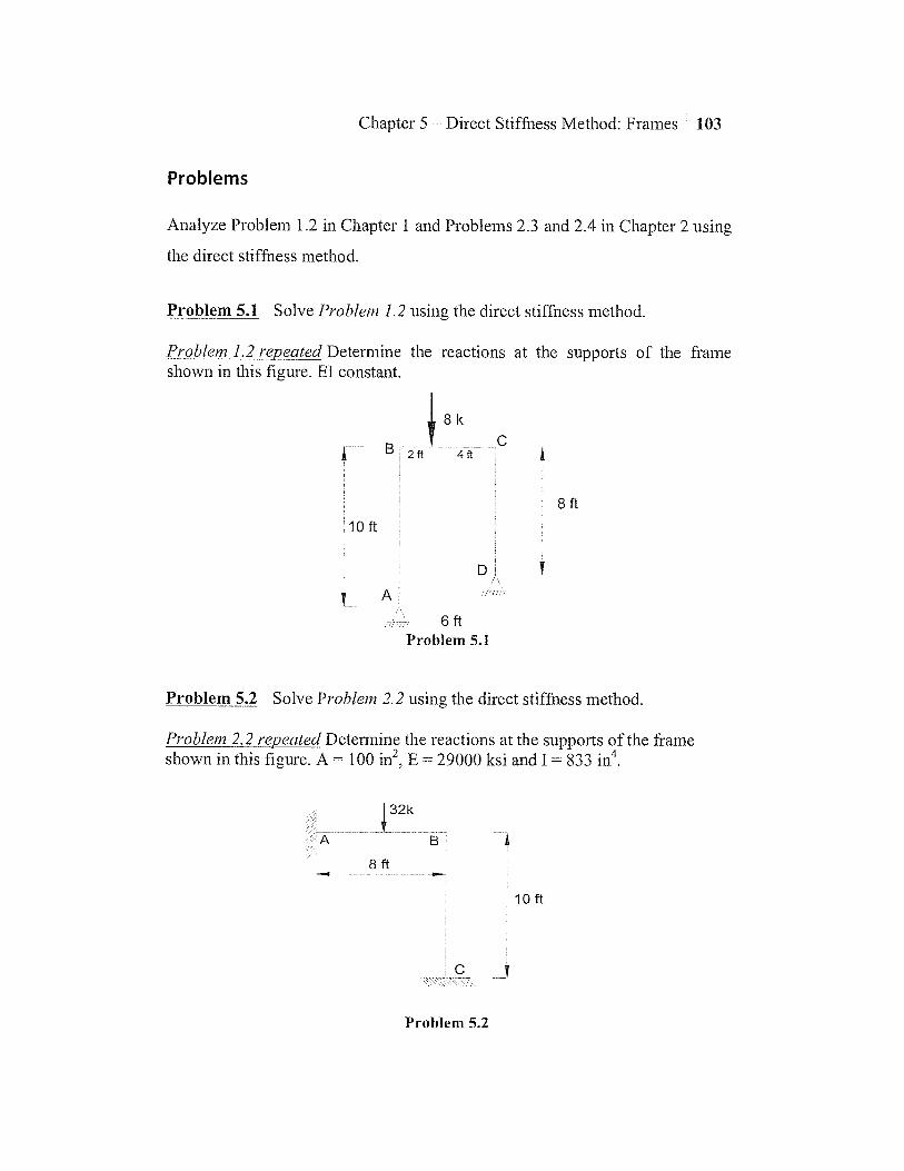
Chapter 5 — Direct Stiffness Method: Frames 103
Problems
Analyze Problem 1.2 in Chapter 1 and Problems 2.3 and 2.4 in Chapter 2 using
the direct stiffness method.
Problem 5.1 Solve Problem 1.2 using the direct stiffness method.
Problem 1.2 repeated Determine the reactions at the supports of the frame shown in this figure. EI constant.
8k
B 2ft 4ft
8 ft 10ft
6ft Problem 5.1
Problem 5.2 Solve Problem 2.2 using the direct stiffness method.
Problem 2.2 repeated Determine the reactions at the supports of the frame shown in this figure. A = 100 in2, E = 29000 ksi and I = 833 in4.
10 ft
Problem 5.2

104 Chapter 5 — Direct Stiffness Method: Frames
Problem 5.3 Solve Problem 2.3 using the direct stiffness method.
Problem 2.3 repeated Determine the reactions at the supports of the frame shown in this figure. A = 100 in2, E = 29000 ksi and I = 833 in4
32 k
B
2 ft
10 ft
8 ft
Problem 5.3

Chapt2 6
Direct Stiffness Method: Application to Trusses
6.1 Derivation/Explanation of the Stiffness Matrix for a Truss Element
As stated earlier, the basic procedure of direct stiffness method has
been explained in Chapter 4. The explanation is essentially a general
procedure, which is also applicable to trusses. The only difference is that in the
case of a truss, the element stiffness matrix [K] for a truss element has to be
used instead of that for a beam element. It should also be noted that the
members of a truss are subjected to tension or compressive forces only as all
the loads on the truss are nodal loads and not member loads. This means that
the members of the truss are not subjected to any bending. While this doesn't
make any difference in application of the direct stiffness method, it is an
important point to be noted. This concept will be clearer once an example of a
truss is solved using the direct stiffness method. Consider the general truss
element shown in Fig. 6.1.
A4, D4
A3, D3
Figure 6.1: Typical truss element with free and restrained supports

106 Chapter 6 — Direct Stiffness Method: Trusses
The member stiffness matrix for the truss element in structural (global) coordinates, [Kmsi ] is given in Eq. 6.1 as,
Equation 6.1: Truss element stiffness matrix
DI D2 D3 D4
Cx2 Cx Cy -Cx 2 Cx Cy Al
AE Cx Cy Cy 2 Cx Cy -Cy2 A2 [Kmsi] = T (6.1)
—Cx 2 —Cx Cy Cx 2 Cx Cy A3
— Cx Cy — Cy 2 Cx Cy Cy 2 A4
Where, Cx and Cy are the direction cosines of the members given as (see Fig.
6.1 for reference),
Cx (xk - x j) (6.2)
C = (Yk - Yj) (6.3)
EA is the usual axial rigidity of the truss member. The global stiffness
matrix [KMSI ] shown in Eq. 6.1 relates the action vector {Ai, A2, A3, A4}t to the
displacement vector {D1, D2, D3, DJ.
Again, like in the case of the beam, some of the elements of the
displacement vector will be zero and will correspond to {DR }, the restrained
displacement vector, which is subset of the {D) vector. Similarly, the
unknown, or free, displacements will be part of the free displacement vector
(DF), which is also a subset of the total displacement vector (D).

Chapter 6 — Direct Stiffness Method: Trusses 107
6.2 Application of the Direct Stiffness Method to a Truss
The process used to solve for the reactions of an indeterminate truss using the
direct stiffness method is explained below using Example 6.2.1.
Example 6.2.1
Determine the reactions at the support of the truss shown in Fig. 6.2 using direct stiffness method. AE is constant.
4 ft
Figure 6.2: Indeterminate truss
Step 1-3
These steps are shown in Fig. 6.3. Figure 6.3 shows that the KI
(Kinematic Indeterminacy) of this structure is 2. Thus, the (DF} vector is:
(Di, D2}. In this problem, just as in the beam and frame problem, the
numbering of the displacements is done starting with the free
displacements. The restrained displacement vector for this problem [DR } is
Ws, D4, D5, D6, D7, D8). Only the free displacements are to be obtained
from [KFF ] and the fAFN) as a solution of the problem.

108 Chapter 6 — Direct Stiffness Method: Trusses
4k
Figure 6.3: Truss showing displacements
Step 4
The member stiffness matrix [K1] for member 1 is obtained using Eq. 6.1.
It isgiven as,
Table 6.1: Truss member stiffness matrix for member 1 1 2 3 4
0.333 0 -0.333 0
0 0 0 0 [K1] = AE
-0.333 0 0.333 0
0 0 0 0
Similarly, the stiffness matrix for member 2 [K2] is given as,
Table 6.2: Truss member stiffness matrix for member 2 1 2 5 6
0.072 0.096 -0.072 -0.096
0.096 0.128 -0.096 -0.128 [K2] = AE
-0.072 -0.096 0.072 0.096
-0.096 -0.128 0.096 0.128

Chapter 6 — Direct Stiffness Method: Trusses 109
Finally, the stiffness matrix for member 3 [K3] is given as,
Table 6.3: Truss member stiffness matrix for member 3
[K3] = AE
3
0
0
0
0
4
0
0.25
0
-0.25
5
0
0
0
0
6
0
-0.25
0
0.25
Combining the three member stiffness matrices yields the structure
stiffness matrix given below in Table 6.4.
Table 6.4: Truss structure stiffness matrix 1 2 3 5 6
0.405 0.096 -0.333 0 -0.072 -0.096
0.096 0.128 0 0 -0.096 -0.128
-0.333 0 0.333 0 0 0 [Kj i = AE
0 0 0 0.25 0 -0.25
-0.072 -0.096 0 0 0.072 0.096
-0.096 -0.128 0 -0.25 0.096 0.378
Step 5
Since just the unknown displacements are to be obtained in this
problem, we only need [KFF ] and {AFN) corresponding to the free
displacements.
From the given condition, we can calculate:
{AFN} — t 04) 21

110 I Chapter 6 — Direct Stiffness Method: Trusses
From [K], we can derive [KFF ]:
AE 10.405 0.0961 [KFF] I-0.096 0.1281
We can solve the displacement:
[KFF]_' {AFN) = ATI" {__9381
Calculate the reaction forces:
-A3- A4 A5
_A6_
—3 kips- ()
3 kips 4 kips _
- [KRF] PA. -
In this problem there is only one nodal load (at joint 4). So, the
assembly of (AFN ) is rather simple. However, if there are other loads at
other nodes or if there are some support settlements, the corresponding
{AFN } vector should be assembled accordingly.
This completes the solution of the problem.

Chapter 6 — Direct Stiffness Method: Trusses 111
6.3 Summary
In this chapter, the powerful method called the direct stiffness method
has been applied to a truss problem. The point to be noted about the direct
stiffness method is that it can be applied to structures that are mainly in flexure
(bending) like beams and frames, as well as structures in tension or
compression (like a trusses). The method essentially is the same except that the
truss element stiffness matrix is used in analysis of trusses as opposed to a
beam or frame element stiffness matrix.
Hence, the direct stiffness method is so powerful and popular that it is
used for almost all the computer codes prevalent in structural analysis.

112 I Chapter 6 — Direct Stiffness Method: Trusses
Problems
Analyze Problem 1.3 in Chapter 1 using the direct stiffness method.
Problem 6.1 Solve Problem 1.3 using the direct stiffness method.
Problem 1.3 repeated Determine the reactions at the supports of the truss shown in this figure. AE is constant.
10 kN
D
C
4m Problem 6.1

L2
Pab 2 Pa2b L2 MFBA = MFAB =
2PL MFAB =
2PL MFBA = 9
6EIL MFBA = L2
L
MFAB = (7,7)(b2a +c)
P
wL2 MFAB = 12
wL2 MFBA = 12
WL2 MFAB = 20
wL2 MFBA = 38
6E/A MFAB = L2 3E/A
MFAB = L2
L wL2
MFAB = 8
wL2 MFAB = —15
.•• ppen©ii
Table 1A: Fixed-End Moments
Both Ends Fixed Far End Pinned

References
Chajes, A. (1983). Structural Analysis. Prentice-Hall, Inc., Englewood Cliffs,
NJ.
Hibbeler, R.C. (2012). Structural Analysis. Prentice Hall, Upper Saddle
River, New Jersey.
Wang. C-K. (1953). Statically Indeterminate Structures. McGraw-Hill Book
Company. New York.
Weaver,W. and Gere, J.M. (1990). Matrix Analysis of Framed Structures.
McGraw-Hill Van Nostrand Reinhold, New York.


Kenneth Derucher
Dr. Kenneth Derucher is a Professor of Civil Engineering at California State University, Chico (Chico State) and served as the Dean of the College of Engineering, Computer Science, and Construction Management at Chico State from 1994-2008. Dr. Derucher is a Professional Engineer (Structural) who is licensed in Washington, D.C.
Chandrasekhar Putcha
Dr. Chandrasekhar Putcha is a Professor in the Department of Civil and Environmental Engineering at California State University, Fullerton.
Uksun Kim
Dr. Uksun Kim is an Associate Professor and Chair of Civil and Environmental Engineering at California State University, Fullerton. He earned his Ph.D. from the School of Civil and Environmental Engineering at Georgia Institute of Technology, Atlanta.


![Sidesway Web Buckling of Steel Beams[1]](https://static.fdocuments.us/doc/165x107/55cf92b2550346f57b98d6e6/sidesway-web-buckling-of-steel-beams1.jpg)