1

Incorporating Contextual Information in Recommender Systems Using a Multidimensional Approach

Gediminas Adomavicius

Department of Information & Decision Sciences Carlson School of Management

University of Minnesota gedas@umn.edu

Ramesh Sankaranarayanan

Department of Information, Operations & Management Sciences Stern School of Business

New York University rsankara@stern.nyu.edu

Shahana Sen

Marketing Department Silberman College of Business Fairleigh Dickinson University

sen@fdu.edu

Alexander Tuzhilin Department of Information, Operations & Management Sciences

Stern School of Business New York University

atuzhili@stern.nyu.edu

Abstract The paper presents a multidimensional (MD) approach to recommender systems that can provide recommendations based on additional contextual information besides the typical information on users and items used in most of the current recommender systems. This approach supports multiple dimensions, extensive profiling, and hierarchical aggregation of recommendations. The paper also presents a multidimensional rating estimation method capable of selecting two-dimensional segments of ratings pertinent to the recommendation context and applying standard collaborative filtering or other traditional two-dimensional rating estimation techniques to these segments. A comparison of the multidimensional and two-dimensional rating estimation approaches is made, and the tradeoffs between the two are studied. Moreover, the paper introduces a combined rating estimation method that identifies the situations where the MD approach outperforms the standard two-dimensional approach and uses the MD approach in those situations and the standard two-dimensional approach elsewhere. Finally, the paper presents a pilot empirical study of the combined approach, using a multidimensional movie recommender system that was developed for implementing this approach and testing its performance.

2

1. Introduction and Motivation There has been much work done in the area of recommender systems over the past decade since the introduction of the first papers on the subject [Resnick et al. 1994; Hill et al. 1995; Shardanand & Maes 1995]. Most of this work has focused on developing new methods of recommending items to users and vice versa, such as recommending movies to Web site visitors or recommending customers for books. These recommendation methods are usually classified into collaborative, content-based and hybrid methods [Balabanovic & Shoham 1997] and are described in more detail in Section 2. However, in many applications, such as recommending a vacation package, personalized content on a Web site, various products in an online store, or a movie, it may not be sufficient to consider only users and items – it is also important to incorporate the contextual information into the recommendation process. For example, in case of personalized content delivery on a Web site, it is important to determine what content needs to be delivered (recommended) to a customer and when. More specifically, on weekdays a user might prefer to read world news when she logs on in the morning and the stock market report in the evening, and on weekends to read movie reviews and do shopping. As another example of the need for the contextual information, a “smart” shopping cart providing real-time recommendations to shoppers using wireless location-based technologies [Wade 2003] needs to take into account not only information about products and customers but also such contextual information as shopping date/time, store, who accompanies the primary shopper, products already placed into the shopping cart and its location within the store. As still another example, a recommender system may recommend to a user a different movie depending on whether she is going to see it with her boyfriend on a Saturday night or with her parents on a weekday. These observations are consistent with the findings in behavioral research on consumer decision making in marketing that have established that decision making, rather than being invariant, is contingent on the context of decision making. In particular, the same consumer may use different decision-making strategies and prefer different products or brands under different contexts [Lussier & Olshavsky 1979, Klein & Yadav 1989, Bettman et al. 1991]. Therefore, accurate prediction of consumer preferences undoubtedly depends upon the degree to which we have incorporated the relevant contextual information into a recommendation method. To provide recommendations based on contextual information, we present a multidimensional recommendation model (MD model) that makes recommendations based on multiple dimensions and, therefore, extends the classical two-dimensional (2D) Users×Items paradigm. The MD model was introduced in an earlier workshop paper [Adomavicius & Tuzhilin 2001], where only the preliminary ideas of the MD model were described. In this paper, we present the MD model in a significantly greater depth and also describe various additional aspects, including a formulation of the MD recommendation problem and the analysis of rating aggregation capabilities of the MD model. Moreover, we present a particular rating estimation method for the MD model, and an algorithm that combines the MD and the 2D approaches and provides rating estimations based on the combined approach. Finally, we present a case study of implementing and testing our methods on a movie recommendation application that takes into consideration the contextual multidimensional information, such as when the movie was seen, with whom and where.

3

Since traditional collaborative filtering systems assume homogeneity of context, they usually utilize all the collected ratings data to determine appropriate recommendations. In contrast to this, the main rating estimation method presented in the paper utilizes the reduction-based approach which uses only the ratings that pertain to the context of the user-specified criteria in which a recommendation is made. For example, to recommend a movie to a person who wants to see it in a movie theater on a Saturday night, our method will use only the ratings of the movies seen in the movie theaters over the weekends, if it is determined from the data that the place and the time of the week dimensions affect the moviegoers’ behavior. Moreover, this method combines some of the multi-strategy and local machine learning methods [Atkeson et al., 1997, Fan and Li, 2003, Hand et al. 2001(Sections 6.3.2-6.3.3)] with On-Line Analytical Processing (OLAP) [Kimball 1996; Chaudhuri & Dayal 1997] and marketing segmentation methods [Kotler 2003] to predict unknown ratings. We also show in the paper that there is a tradeoff between having more pertinent data for calculating an unknown rating and having fewer data points used in this calculation based only on the ratings with the same or similar context, i.e., the tradeoff between greater pertinence vs. higher sparsity of the data. We also show how to achieve better recommendations using this tradeoff. The contributions of this paper lie in:

• Presenting the multidimensional recommendation model and studying some of its properties and capabilities.

• Proposing a multidimensional rating estimation method based on a reduction-based approach that segments the ratings based on user-specified criteria and then applies collaborative filtering or other two-dimensional rating estimation methods to the resulting two-dimensional segment.

• Demonstrating that context matters, i.e., that the multidimensional approach can produce better rating estimations for the reduction-based approach in some situations. Furthermore, we demonstrate that context might matter only in some cases and not in others, i.e., that the reduction-based approach outperforms the 2D approach in some situations (on some contextual segments of the data) and underperforms in others.

• Proposing a combined approach that identifies the contextual segments where the reduction-based approach outperforms the 2D approach and using this approach in these situations, and the standard 2D approach in the rest.

• Implementing the combined approach and empirically demonstrating that this combined approach outperforms the standard 2D collaborative filtering approach on the multidimensional rating data that we collected (by designing a Web site for this purpose).

• Proposing, from the machine learning perspective, to apply local machine learning methods and to combine them with OLAP and market segmentation methods to identify local regions where local models predicting unknown ratings are built. Moreover, we use a multi-strategy machine learning method to combine local and global models to achieve better predictions of unknown ratings.

Before presenting the MD approach in Section 3 and an MD rating estimation method in Section 4, we first review the prior work on recommender systems in Section 2.

4

2. Prior Work on Recommender Systems Traditionally, recommender systems deal with applications that have two types of entities, users and items. The recommendation process starts with the specification of the initial set of ratings that is either explicitly provided by the users or is implicitly inferred by the system. For example, in case of a movie recommender system, John Doe may assign a rating of 7 (out of 13) for the movie “Gladiator,” i.e., set Rmovie(John_Doe, Gladiator)=7. Once these initial ratings are specified, a recommender system tries to estimate the rating function R

R: Users × Items → Ratings (1) for the (user, item) pairs that have not been rated yet by the users. Conceptually, once function R is estimated for the whole Users×Items domain, a recommender system can select the item ui′ with the highest rating (or a set of k highest-rated items) for user u and recommend that item(s) to the user, i.e.,

, arg max ( , )ui Items

u Users i R u i∈

′∀ ∈ = (2)

In practice, however, the unknown ratings do not have to be estimated for the whole Users×Items space beforehand, since this can be a very expensive task for large domains of users and items. Instead, various methods have been developed for finding efficient solutions to (2) requiring smaller computational efforts, e.g., as described in [Goldberg et al. 2001; Sarwar et al. 2001]. According to [Balabanovic & Shoham 1997], the approaches to recommender systems are usually classified as content-based, collaborative, and hybrid, and we review them in the rest of this section. Content-based Recommender Systems. In content-based recommendation methods, the rating R(u,i) of item i for user u is typically estimated based on the ratings R(u,i') assigned by the same user u to other items i'∈Items that are “similar” to item i in terms of their content. For example, in a movie recommendation application, in order to recommend movies to user u, the content-based recommender system tries to understand user preferences by analyzing commonalities among the content of the movies user u has rated highly in the past. Then, only the movies that have a high degree of similarity to whatever the customer’s preferences are would get recommended.

More formally, let Content(i) be the set of attributes characterizing item i. It is usually computed by extracting a set of features from item i (its content) and is used to determine appropriateness of the item for recommendation purposes. Since many content-based systems are designed for recommending text-based items, including Web pages and Usenet news messages, the content in these systems is usually described with keywords, as is done in the Fab [Balabanovic & Shoham 1997] and the Syskill & Webert [Pazzani & Billsus 1997] recommender systems. The “importance” of a keyword is determined with some weighting measure that can be defined using various measures from information retrieval [Salton 1989; Baeza-Yates & Ribeiro-Neto 1999], such as term frequency/inverse document frequency (TF-IDF) measure [Salton 1989].

5

In addition, we need to define a profile of user u. Since many content systems deal with recommending text-based items, these user profiles are also often defined in terms of weights of important keywords. In other words, ContentBasedProfile(u) for user u can be defined as a vector of weights (wu1, …, wuk), where each weight wui denotes the importance of keyword ki to user u and can also be specified using various information retrieval metrics, including the TF-IDF measure [Lang 1995; Pazzani & Billsus 1997].

In content-based recommender systems the rating function R(u,i) is usually defined as

( , ) ( ( ), ( ))R u i score ContentBasedProfile u Content i= (3)

In case ContentBasedProfile(u) and Content(i) are defined as vectors of keyword weights uw and

iw , as is usually done for recommending Web pages, Usenet messages, and other kinds of textual documents, rating function R(u,i) is usually represented in information retrieval literature by some scoring heuristic defined in terms of vectors uw and iw , such as the cosine similarity measure [Salton 1989; Baeza-Yates & Ribeiro-Neto 1999].

Besides the traditional heuristics that are based mostly on information retrieval methods, other techniques for content-based recommendations have also been used, such as Bayesian classifiers [Pazzani & Billsus 1997; Mooney et al. 1998] and various machine learning techniques, including clustering, decision trees, and artificial neural networks [Pazzani & Billsus 1997]. These techniques differ from information retrieval-based approaches in that they calculate estimated ratings based not on a heuristic formula, such as the cosine similarity measure, but rather are based on a model learned from the underlying data using statistical learning and machine learning techniques. For example, based on a set of Web pages that were rated as “relevant” or “irrelevant” by the user, Pazzani & Billsus [1997] use the naïve Bayesian classifier [Duda et al. 2001] to classify unrated Web pages. As was observed in [Shardanand & Maes 1995; Balabanovic & Shoham 1997], content-based recommender systems have several limitations. Specifically content-based recommender systems have only limited content analysis capabilities [Shardanand & Maes 1995]. In other words, such recommender systems are the most useful in the domains, where content information can be extracted automatically (e.g., using various feature extraction methods on textual data) or where it has been provided manually (e.g., information about movies). It would be much more difficult to use such systems to recommend, say, multimedia items (e.g., audio and video streams) that are not manually “annotated” with context information. Content-based recommender systems can also suffer from over-specialization, since, by design, the user is being recommended only the items that are similar to the ones she rated highly in the past. However, in certain cases, items should not be recommended if they are too similar to something the user has already seen, such as a different news article describing the same event. Therefore, some content-based recommender systems, such as DailyLearner [Billsus & Pazzani 2000], filter out high-relevance items if they are too similar to something the user has seen before. Finally, the user has to rate a sufficient number of items before a content-based recommender system can really understand her preferences and present reliable recommendations. This is often referred to

6

as a new user problem, since a new user, having very few ratings, often is not able to get accurate recommendations. To address some of these issues, the collaborative filtering approach [Resnick et al. 1994; Hill et al. 1995; Shardanand & Maes 1995] has been used in recommender systems. Collaborative Recommender Systems. Traditionally, many collaborative recommender systems try to predict the rating of an item for a particular customer based on how other customers previously rated the same item. More formally, the rating R(u,i) of item i for user u is estimated based on the ratings R(u’,i) assigned to the same item i by those users u’ who are “similar” to user u. There have been many collaborative systems developed in academia and industry since the development of the first systems, such as GroupLens [Resnick et al. 1994; Konstan et al. 1997], Video Recommender [Hill et al. 1995], and Ringo [Shardanand & Maes 1995], that used collaborative filtering algorithms to automate the recommendation process. Other examples of collaborative recommender systems include the book recommendation system from Amazon.com, MovieCritic that recommends movies on the Web, the PHOAKS system that helps people find relevant information on the Web [Terveen et al. 1997], and the Jester system that recommends jokes [Goldberg et al. 2001]. According to Breese et al. [1998], algorithms for collaborative recommendations can be grouped into two general classes: memory-based (or heuristic-based) and model-based. Memory-based algorithms [Resnick et al. 1994; Shardanand & Maes 1995; Breese et al. 1998; Nakamura & Abe 1998; Delgado & Ishii 1999] are heuristics that make rating predictions based on the entire collection of previously rated items by the users. That is, the value of the unknown rating ru,i for user u and item i is usually computed as an aggregate of the ratings of some other (e.g., the N most similar) users for the same item i:

, ,

ˆaggru i u i

u Ur r ′

′∈= (4)

where U denotes the set of N users u′ that are the most similar to user u and who have rated item i (N can range anywhere from 1 to the number of all users). Some examples of the aggregation function are:

, , , , , ,ˆ ˆ ˆ

1(a) (b) ( , ) (c) ( , ) ( )u i u i u i u i u i u u i uu U u U u U

r r r k sim u u r r r k sim u u r rN ′ ′ ′ ′

′ ′ ′∈ ∈ ∈

′ ′= = × = + × −∑ ∑ ∑

(5a, 5b, 5c) where multiplier k serves as a normalizing factor and is usually selected as

ˆ1 | ( , ) |u U

k sim u u′∈

′= ∑ , and where the average rating of user u, ur , in (5c) is defined as

( ) ,1 | |u

u u u ii Sr S r

∈= ∑ , where ,{ | }u u iS i r ε= ≠ 1.

1 We use the ,i jr ε= notation to indicate that item j has not been rated by user i.

7

The similarity measure between the users u and u’, sim(u, u’), determines the “distance” between users u and u’ and is used as a weight for ratings ,u ir ′ , i.e., the more similar users u and u’ are, the more weight rating ,u ir ′ will carry in the prediction of ,u ir . Various approaches have been used to compute similarity measure ( , )sim u u′ between users in collaborative recommender systems. In most of these approaches, ( , )sim u u′ is based on the ratings of items that both users u and u’ have rated. The two most popular approaches are the correlation-based [Resnick et al. 1994; Shardanand & Maes 1995]:

, ,

2 2, ,

( )( )( , )

( ) ( )xy

xy xy

x s x y s ys S

x s x y s ys S s S

r r r rsim x y

r r r r∈

∈ ∈

− −

=− −

∑

∑ ∑ (6)

and the cosine-based [Breese et al. 1998; Sarwar et al. 2001]:

, ,

2 22 2 , ,

( , ) cos( , )|| || || ||

xy

xy xy

x s y ss S

x s y ss S s S

r rx ysim x y x y

x y r r∈

∈ ∈

⋅= = =

×

∑

∑ ∑ (7)

where rx,s and ry,s are the ratings of item s assigned by users x and y respectively, , ,{ | }xy x s y sS s Items r rε ε= ∈ ≠ ∧ ≠ is the set of all items co-rated by both customers x and y, and

x y⋅ denotes the dot-product between the vectors x and y . Many performance-improving modifications, such as default voting, inverse user frequency, case amplification [Breese et al. 1998], and weighted-majority prediction [Nakamura & Abe 1998; Delgado & Ishii 1999], have been proposed as extensions to these standard correlation-based and cosine-based techniques. Moreover, [Aggarwal et al. 1999] propose a graph-theoretic approach to collaborative filtering where similarities between users are calculated in advance and are stored as a directed graph. Also, while the above techniques traditionally have been used to compute similarities between users, [Sarwar et al. 2001] proposed to use the same correlation-based and cosine-based techniques to compute similarities between items instead and to obtain ratings from them. Furthermore, Sarwar et al. [2001] argue that item-based algorithms can provide better computational performance than traditional user-based collaborative methods, while at the same time also providing better quality than the best available user-based algorithms. In contrast to memory-based methods, model-based algorithms [Breese et al. 1998; Billsus & Pazzani 1998; Ungar & Foster 1998; Chien & George 1999; Getoor & Sahami 1999; Goldberg et al. 2001] use the collection of ratings to learn a model, which is then used to make rating predictions. Therefore, in comparison to model-based methods, the memory-based algorithms can be thought of as “lazy learning” methods in the sense that they do not build a model and perform the heuristic computations at the time recommendations are sought. One example of model-based recommendation techniques is presented in [Breese et al. 1998], where a probabilistic approach to collaborative filtering is proposed and the unknown ratings are calculated as

8

, , , ,0

( ) Pr( | , )n

u i u i u i u i ux

r E r x r x r i S′=

′= = × = ∈∑ (8)

and it is assumed that rating values are integers between 0 and n, and the probability expression is the probability that user u will give a particular rating to item i given the previous ratings of items rated by user u. To estimate this probability, [Breese et al. 1998] proposes two alternative probabilistic models: cluster models and Bayesian networks. Moreover, [Billsus & Pazzani 1998] proposed a collaborative filtering method in a machine learning framework, where various machine learning techniques (such as artificial neural networks) coupled with feature extraction techniques (such as singular value decomposition – an algebraic technique for reducing dimensionality of matrices) can be used. Dimensionality reduction techniques for recommender systems were also studied in [Sarwar et al. 2000]. Furthermore, both [Breese et al. 1998] and [Billsus & Pazzani 1998] compare their respective model-based approaches with standard memory-based approaches and report that model-based methods in some instances can outperform memory-based approaches in terms of accuracy of recommendations. There have been several other model-based collaborative recommendation approaches proposed in the literature. A statistical model for collaborative filtering was proposed in [Ungar & Foster 1998], and several different algorithms for estimating the model parameters were compared, including K-means clustering and Gibbs sampling. Other methods for collaborative filtering include a Bayesian model [Chien & George 1999], a probabilistic relational model [Getoor & Sahami 1999], and a linear regression [Sarwar et al. 2001]. Also, a method combining both memory-based and model-based approaches was proposed in [Pennock & Horvitz 1999], where it was empirically demonstrated that the use of this combined approach can provide better recommendations than pure memory-based and model-based approaches. Furthermore, [Kumar et al. 2001] use simple probabilistic model for collaborative filtering to demonstrate that recommender systems can be valuable even with little data on each user, and that simple algorithms can be almost as effective as the best possible ones in terms of utility. Although the pure collaborative recommender systems do not have some of the shortcomings of the content-based systems described earlier, such as limited content analysis or over-specialization, they do have other limitations [Balabanovic & Shoham 1997; Lee 2001]. In addition to the new user problem (the same issue as in content-based systems), the collaborative recommender systems also tend to suffer from the new item problem, since they rely solely on rating data to make recommendations. Therefore, the recommender system would not be able to recommend a new item until it is rated by a substantial number of users. The sparsity of ratings is another important problem that collaborative recommender systems frequently face, since the number of user-specified ratings is usually very small compared to the number of ratings that need to be predicted. For example, in the movie recommendation system there may be many movies that have been rated only by few people and these movies would be recommended very rarely, even if those few users gave high ratings to them. Also, for the user whose tastes are unusual compared to the rest of the population there may not be any other users who are particularly similar, leading to poor recommendations [Balabanovic & Shoham 1997]. To

9

address some of these problems, some researchers proposed to combine the content-based and collaborative approaches into a hybrid approach. Hybrid Recommender Systems. Content and collaborative methods can be combined together into the hybrid approach in several different ways [Balabanovic & Shoham 1997; Basu et al. 1998; Ungar & Foster 1998; Claypool et al. 1999; Soboroff & Nicholas 1999; Pazzani 1999; Tran & Cohen 2000]. Many hybrid recommender systems, including Fab [Balabanovic & Shoham 1997] and the “collaboration via content” approach described in [Pazzani 1999], combine collaborative and content-based approaches by (1) learning and maintaining user profiles based on content analysis using various information retrieval methods and/or other content-based techniques, and (2) directly comparing the resulting profiles to determine similar users in order to make collaborative recommendations. This means that users can be recommended items when items either score highly against the user’s profile or are rated highly by a user with a similar profile. Basu et al. [1998] follow a similar approach and propose the use of additional sources of information, such as the age , gender of users and the genre of movies, to aid collaborative filtering predictions. This amounts to adding some content-based elements to the collaborative filtering method. Also, [Soboroff & Nicholas 1999] proposes to use the latent semantic indexing technique to incorporate and conveniently rearrange the collaborative information, such as the collection of user profiles, in the content-based recommendation framework. This enables comparison of items (e.g., textual documents) and user profiles in a unified model; as the result, the commonalities between users can be exploited in the content filtering task. Another approach to building hybrid recommender systems is to implement separate collaborative and content-based recommender systems. Then, we can have two different scenarios. First, we can combine the outputs (ratings) obtained from individual recommender systems into one final recommendation using either a linear combination of ratings [Claypool et al. 1999] or a voting scheme [Pazzani 1999]. Alternatively, we can use one of the individual recommender systems, at any given moment choosing to use the one that is “better” than others based on some recommendation quality metric. For example, the DailyLearner system [Billsus & Pazzani 2000] selects the recommender system that can give the recommendation with the higher level of confidence, while [Tran & Cohen 2000] chooses the one whose recommendation is more consistent with past ratings of the user.

Yet another hybrid approach to recommendations is used by [Condliff et al. 1999; Ansari et al. 2000], where instead of combining collaborative and content-based methods the authors propose to use information about both users and items in a single recommendation model. Both [Condliff et al. 1999] and [Ansari et al. 2000] use Bayesian mixed-effects regression models that employ Markov chain Monte Carlo methods for parameter estimation and prediction.

Finally, it was demonstrated in [Balabanovic & Shoham 1997; Pazzani 1999] that hybrid methods can provide more accurate recommendations than pure collaborative and content-based approaches.

10

All of the approaches described in this section focus on recommending items to users or users to items and do not take into the consideration additional contextual information, such as time, place, the company of other people, and other factors described in Section 1 affecting recommendation experiences. Moreover, the recommendation methods are hard-wired into these recommendation systems and provide only particular types of recommendations. To address these issues, [Adomavicius & Tuzhilin 2001] proposed a multidimensional approach to recommendations where the traditional two-dimensional user/item paradigm was extended to support additional dimensions capturing the context in which recommendations are made. This multidimensional approach is based on the multidimensional data model used for data warehousing and On-Line Analytical Processing (OLAP) applications in databases [Kimball 1996; Chaudhuri & Dayal 1997], on hierarchical aggregation capabilities, and on user, item and other profiles defined for each of these dimensions. Moreover, [Adomavicius & Tuzhilin 2001] also describes how the standard multidimensional OLAP model is adjusted when applied to recommender systems. Finally, to provide more extensive and flexible types of recommendations that can be requested by the user on demand, [Adomavicius & Tuzhilin 2001] presented a Recommendation Query Language (RQL) that allows users to express complex recommendations that can take into account multiple dimensions, aggregation hierarchies, and extensive profiling information. The usage of contextual information in recommender systems can also be traced to [Herlocker & Konstan 2001], who argued that the inclusion of knowledge about user’s task into the recommendation algorithm in certain applications can lead to better recommendations. For example, if we want to recommend books as gifts for a child, then, according to [Herlocker & Konstan 2001], we might want to use several books that the child already has and likes and use this information in calculating new recommendations. However, this approach is still two-dimensional (i.e., it uses only User and Item dimensions), since the task specification consists of a list of sample items and no additional contextual dimensions are used. However, this approach was successful in illustrating the value of incorporating additional information into the standard collaborative filtering paradigm. Our proposal to incorporate other dimensions into recommender systems is in line with the research on consumer decision making by behavioral researchers who have established that decision making, rather than being invariant, is contingent on the context of the decision making. The same consumer may use different decision-making strategies and prefer different products or brands, under different contexts [Bettman et al. 1991]. According to [Lilien et al. 1992], “consumers vary in their decision-making rules because of the usage situation, the use of the good or service (for family, for gift, for self) and purchase situation (catalog sale, in-store shelf selection, salesperson aided purchase).” Therefore accurate prediction of consumer preference undoubtedly depends upon the degree to which we have incorporated the relevant contextual information (e.g. usage situation, purchase situation, who is it for, etc.) in a recommender system. 3. Multidimensional Recommendation Model (MD Model) In this section, we describe the multidimensional (MD) recommentation model consisting of three main components: multiple dimensions, profiles for each dimension, and rating aggregation capabilities. We describe each of these components below.

11

3.1 Multiple Dimensions As stated before, the MD model provides recommendations not only over the User×Item dimensions, as the classical (2D) recommender systems do, but over several dimensions, such as User, Item, Time, Place, etc. When considering multiple dimensions, we will follow the multidimensional data model used for data warehousing and OLAP applications in databases [Kimball 1996; Chaudhuri & Dayal 1997]. Formally, let D1, D2, …, Dn be dimensions, each dimension Di being a subset of a Cartesian product of some attributes (or fields) Aij, (j = 1,…,ki), i.e., Di ⊆ Ai1× Ai2 × …× Aiki, where each attribute defines a domain (or a set) of values. Moreover, one or several attributes form a key, i.e., they uniquely define the rest of the attributes [Ramakrishnan & Gehrke 2000]. In some cases a dimension can be defined by a single attribute, and ki=1 in such cases 2 . Given dimensions D1, D2, …, Dn, we define the recommendation space for these dimensions as a Cartesian product S = D1× D2× …× Dn. Moreover, let Ratings be a rating domain representing the ordered set of all possible rating values. Then the rating function is defined over the space

1 nD D× ×… as 1: nR D D Ratings× × →… (9)

Example. Consider the three-dimensional recommendation space User×Item×Time where the User dimension is defined as User ⊆ UName× Address × Income × Age and consists of a set of users having certain names, addresses, incomes, and being of a certain age. Similarly, the Items dimension is defined as Item ⊆ IName× Type × Price and consists of a set of items defined by their names, types and the price. Finally, the Time dimension can be defined as Time ⊆ Year × Month × Day and consists of a list of days from the starting to the ending date (e.g. from January 1, 2003 to December 31, 2003). Then we define a rating function R on the recommendation space User×Item×Time specifying how much user u ∈ User liked item i∈ Item at time t∈ Time, R(u,i,t). For example, John Doe rated a vacation that he took at the Almond Resort Club on Barbados on January 7-14, 2003 as 6 (out of 7).

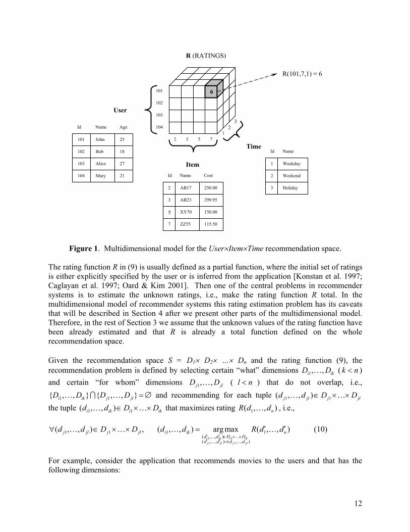
Visually, ratings 1( , , )nR d d… on the recommendation space S = D1× D2× …× Dn can be stored in a multidimensional cube, such as the one shown in Figure 1. For example, the cube in Figure 1 stores ratings R(u,i,t) on the recommendation space User×Item×Time, where the three tables define the sets of users, items and times associated with User, Item and Time dimensions respectively. For example, rating R(101,7,1) = 6 in Figure 1 means that for the user with User ID 101 and the item with Item ID 7, rating 6 was specified during the weekday. 2 To simplify the presentation, we will sometimes not distinguish between “dimension” and “attribute” for single-attribute dimensions and will use these terms interchangeably when it is clear from the context.

12

Figure 1. Multidimensional model for the User×Item×Time recommendation space. The rating function R in (9) is usually defined as a partial function, where the initial set of ratings is either explicitly specified by the user or is inferred from the application [Konstan et al. 1997; Caglayan et al. 1997; Oard & Kim 2001]. Then one of the central problems in recommender systems is to estimate the unknown ratings, i.e., make the rating function R total. In the multidimensional model of recommender systems this rating estimation problem has its caveats that will be described in Section 4 after we present other parts of the multidimensional model. Therefore, in the rest of Section 3 we assume that the unknown values of the rating function have been already estimated and that R is already a total function defined on the whole recommendation space. Given the recommendation space S = D1× D2× …× Dn and the rating function (9), the recommendation problem is defined by selecting certain “what” dimensions 1, ,i ikD D… ( k n< ) and certain “for whom” dimensions 1, ,j jlD D… ( l n< ) that do not overlap, i.e.,

1 1{ , , } { , , }i ik j jlD D D D = ∅… ∩ … and recommending for each tuple 1 1( , , )j jl j jld d D D∈ × ×… … the tuple 1 1( , , )i ik i ikd d D D∈ × ×… … that maximizes rating 1( , , )nR d d… , i.e.,

1 11 1

1 1 1 1( , , )( , , ) ( , , )

( , , ) , ( , , ) arg max ( , , )i ik i ikj jl j jl

j jl j jl i ik nd d D Dd d d d

d d D D d d R d d′ ′ ∈ × ×′ ′ =

′ ′∀ ∈ × × =… …… …

… … … … (10)

For example, consider the application that recommends movies to the users and that has the following dimensions:

User

Item

Time

R (RATINGS)

101

102

103

104

John

Bob

Alice

Mary

25

18

27

21

Id Name Age

2

3

5

7

AB17

AB23

XY70

ZZ55

250.00

299.95

150.00

115.50

Id Name Cost

1

2

3

Weekday

Weekend

Holiday

Id Name

101

102

103

104

2 3 5 7 1

2 3

R(101,7,1) = 6

6

13

• Movie: represents all the movies that can be recommended in a given application; it is defined by attributes Movie(MovieID, Name, Studio, Director, Year, Genre, MainActors).

• Person: represents all the people for whom movies are recommended in an application; it is defined by attributes Person(UserID, Name, Address, Age, Occupation, etc.).

• Place: represents the places where the movie can be seen. Place consists of a single attribute defining the listing of movie theaters and also the choices of the home TV, VCR, and DVD.

• Time: represents the time when the movie can be or has been seen; it is defined by attributes Time(TimeOfDay, DayOfWeek, Month, Year).

• Companion: represents a person or a group of persons with whom one can see the movie. Companion consists of a single attribute having values “alone,” “friends,” “girlfriend/boyfriend,” “family,” “co-workers,” and “others.”

Then the rating assigned to a movie by a person also depends on where and how the movie has been seen, with whom and at what time. For example, the type of movie to recommend to college student Jane Doe can differ significantly depending on whether she is planning to see it on a Saturday night with her boyfriend vs. on a weekday with her parents. Some additional applications where multidimensional recommendations are useful were mentioned in Section 1 and include personalized Web content presentation (having the recommendation space S = User × Content × Time) and a “smart” shopping cart (having the recommendation space S = Customer × Product × Time × Store × Location). An important question is what dimensions should be included in a multidimensional recommendation model. This issue is related to the problem of feature selection that has been extensively addressed in data mining [Liu & Motoda 1998] and statistics [Chatterjee et al. 2000]. To understand the issues involved, consider a simple case of a single-attribute dimension X having two possible values X=h and X=t. If the distributions of ratings for X=h and X=t were the same, then dimension X would not matter for recommendation purposes. For example, assume that the single-attribute Place dimension has only two values Theater and Home. Also assume that the ratings given to the movies watched in the movie theater (Place = Theater) have the same distribution as the ratings for the movies watched at home (Place = Home). This means that the place where movies are watched (at home or in a movie theater) does not affect movie watching experiences and, therefore, the Place dimension can be removed from the MD model. There is a rich body of work in statistics that tests whether two distributions or their moment generating functions are equal [Kachigan 1986], and this work can be applied to our case to determine which dimensions should be kept for the MD model (again, this is equivalent to determining which features to keep and which to drop for data mining and statistical models). Finally, this example can easily be extended to the situations when the attribute (or the whole dimension) has other data types besides binary. While most traditional recommender systems provide recommendations only of one particular type, i.e., “recommend top N items to a user,” multidimensional recommender systems offer many more possibilities, including recommending more than one dimension, as expressed in (10). For example, in the personalized Web content application described above, one could ask for the “best N user/time combinations to recommend for each item,” or the “best N items to recommend for each user/time combination,” or the “best N times to recommend for each user/item

14

combination,” etc. Similarly, in the movie recommender system, one can recommend a movie and a place to see it to a person at a certain time (e.g., tomorrow, Joe should see “Harry Potter” in a movie theater). Alternatively, one can recommend a place and a time to see a movie to a person with a companion (e.g., Jane and her boyfriend should see “About Schmidt” on a DVD at home over the weekend). These examples demonstrate that recommendations in the multidimensional case can be significantly more complex than in the classical 2D case. Therefore, there is a need for a special language to be able to express such recommendations, and [Adomavicius & Tuzhilin 2001] proposed a recommendation query language RQL for the purposes of expressing different types of multidimensional recommendations. However, coverage of the RQL language is outside of the scope of this paper, and the reader is referred to [Adomavicius & Tuzhilin 2001] to learn more about it. 3.2 Profiling Capabilities As stated in Section 3.1, each dimension Di is defined by a set of attributes Aij (j=1,…,ki), and these attributes can be used to provide recommendations. This idea is not new and has been explored by Pazzani [1999], who used demographic information about the users to provide better recommendations. Also, some content-based approaches used keywords for providing recommendations [Mooney et al. 1998; Pazzani & Billsus 1997], where keywords can be viewed as attributes describing a document. Also, [Condliff et al. 1999] and [Ansari et al. 2000] proposed a hybrid approach to rating estimation that uses attributes describing the users and the items to provide recommendations. This set of attributes comprises a simple profile describing a particular instance of a given dimension, such as the profile of a user, a product, or a document. For example, in the latter case the profile of a document can consist of a set of keywords found in this document [Pazzani 1999]. More generally, these simple attribute-based profiles can be extended to more comprehensive profiles containing data mining rules [Adomavicius and Tuzhilin 2001b], sequences, signatures [Cortes et al. 2000] and other profiling methods. However, this topic lies outside of the scope of this paper, and we will refer to it only in Section 6. 3.3 Aggregation Capabilities One of the key characteristics of multidimensional databases is the ability to store measurements (such as sales numbers) in multidimensional cubes, support aggregation hierarchies for different dimensions (e.g., a hierarchical classification of products or a time hierarchy), and provide capabilities to aggregate the measurements at different levels of the hierarchy [Kimball 1996; Chaudhuri & Dayal 1997]. For example, we can aggregate individual sales for the carbonated beverages category for a major soft-drink distributor in the Northwest region over the last month. Our multidimensional recommendation model supports the same aggregation capability as the multidimensional data model. However, there are certain idiosyncrasies pertaining to our model that make it different from the classical OLAP models used in databases [Kimball 1996; Chaudhuri & Dayal 1997]. We describe these aggregation capabilities in the rest of this section.

15

As a starting point, we assume that some of the dimensions Di of the multidimensional recommendation model have hierarchies associated with these dimensions, e.g., the Products dimension can use the standard industrial product hierarchy, such as North American Industry Classification System (NAICS – see www.naics.com), and the Time dimension can use one of the temporal hierarchies, such as minutes, hours, days, months, seasons, etc. For example, in the movie recommendation application described in Section 3.1, all the movies can be grouped into sub-genres, and sub-genres can be further grouped into genres. The Person dimension can be grouped based on the age and/or the occupation, or using one of the standard marketing classifications. Also, all the movie theaters for the Place dimension can be grouped into the “Movie Theater” category, and other categories, such as “TV at home,” “VCR at home” and “DVD at home,” can remain intact. Finally, the Companion dimension does not have any aggregation hierarchy associated with it. As mentioned before, some of the dimensions, such as Time, can have more than one hierarchy associated with it. For example, Time can be aggregated into Days/Weeks/Months/Years or into Days/WeekdaysWeekends hierarchies. Selecting appropriate hierarchies is the standard OLAP problem: either the user has to specify a specific hierarchy or these hierarchies can be learned from the data [Han and Kamber 2001, Ch. 3]. In this paper, we assume that a particular hierarchy has been selected or learned for each dimension already, and we use it in our multidimensional model. Given aggregation hierarchies, the enhanced n-dimensional recommendation model consists of

• Profiles describing each item for each of the n dimensions, as described in Section 3.2. For example, for the Movie dimension, we store profiles of all the movies (including movie title, studio, director, year of release, and genre) in our database.

• Aggregation hierarchies associated with each dimension, as described previously in this section.

• The multidimensional cube of ratings, each dimension being defined by the key for this dimension and storing the available rating information in the cells of the cube. For example, a multidimensional cube of ratings for the recommendation space Users×Items×Time was discussed in Section 3.1 and presented in Figure 1.

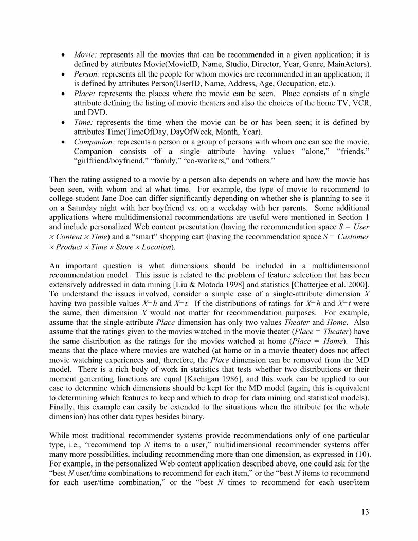
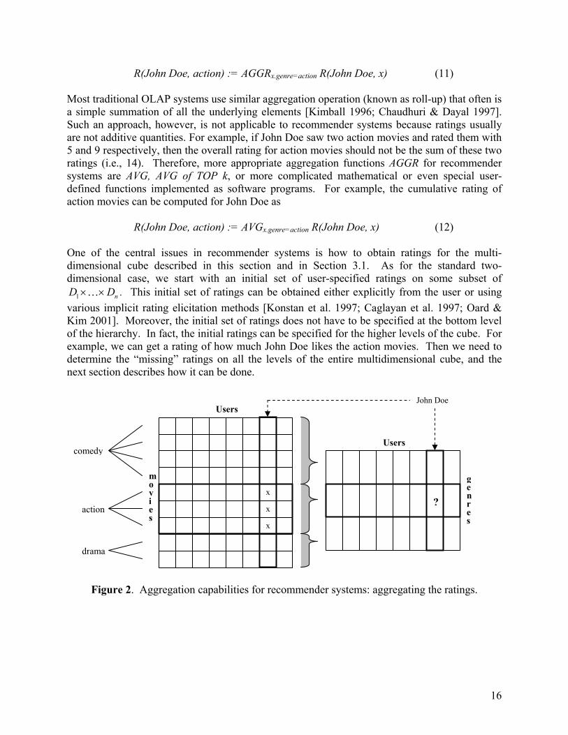
Given this enhanced multidimensional recommendation model defined by the dimensional profiles, hierarchies and a ratings cube, a recommender system can provide more complex recommendations that deal not only with individual items, but also with groups of items. For example, we may want to know not only how individual users like individual movies, e.g., R(John Doe, Gladiator) = 7, but also how they may like categories (genres) of movies, e.g., R(John Doe, action_movies) = 5. Similarly, we may want to group users and other dimensions as well. For example, we may want to know how graduate students like “Gladiator”, e.g., R(graduate_students, Gladiator) = 9. More generally, given individual ratings in the multidimensional cube, we may want to use hierarchies to compute aggregated ratings. For example, assume that movies can be grouped based on their genres and assume that we know how John Doe likes each action movie individually. Then, as shown in Figure 2, we can compute an overall rating of how John Doe likes action movies as a genre by aggregating his individual action movie ratings, i.e.,

16

R(John Doe, action) := AGGRx.genre=action R(John Doe, x) (11) Most traditional OLAP systems use similar aggregation operation (known as roll-up) that often is a simple summation of all the underlying elements [Kimball 1996; Chaudhuri & Dayal 1997]. Such an approach, however, is not applicable to recommender systems because ratings usually are not additive quantities. For example, if John Doe saw two action movies and rated them with 5 and 9 respectively, then the overall rating for action movies should not be the sum of these two ratings (i.e., 14). Therefore, more appropriate aggregation functions AGGR for recommender systems are AVG, AVG of TOP k, or more complicated mathematical or even special user-defined functions implemented as software programs. For example, the cumulative rating of action movies can be computed for John Doe as

R(John Doe, action) := AVGx.genre=action R(John Doe, x) (12) One of the central issues in recommender systems is how to obtain ratings for the multi-dimensional cube described in this section and in Section 3.1. As for the standard two-dimensional case, we start with an initial set of user-specified ratings on some subset of

1 nD D× ×… . This initial set of ratings can be obtained either explicitly from the user or using various implicit rating elicitation methods [Konstan et al. 1997; Caglayan et al. 1997; Oard & Kim 2001]. Moreover, the initial set of ratings does not have to be specified at the bottom level of the hierarchy. In fact, the initial ratings can be specified for the higher levels of the cube. For example, we can get a rating of how much John Doe likes the action movies. Then we need to determine the “missing” ratings on all the levels of the entire multidimensional cube, and the next section describes how it can be done.

Figure 2. Aggregation capabilities for recommender systems: aggregating the ratings.

Users

comedy

action

drama

Users

x

x

x

?

John Doe

m o v i e s

genres

17

4. Rating Estimation in Multidimensional Recommender Systems An important research question is how to estimate unknown ratings in a multidimensional recommendation space. As in traditional recommender systems, the key problem in multidimensional systems is the extrapolation of the rating function from a (usually small) subset of ratings that are specified by the users for different levels of the aggregation hierarchies in the multidimensional cube of ratings. For example, some ratings are specified for the bottom level of individual ratings, such as John Doe assigned rating 7 to “Gladiator,” i.e., R(JD, Gladiator) = 7, whereas others are specified for aggregate ratings, such as John Doe assigned rating 6 to action movies, i.e., R(JD, action) = 6. Then, the general rating estimation problem can be formulated as follows:

Multi-level Multidimensional Rating Estimation Problem: given the initial (small) set of user-assigned ratings specified for different levels of the multidimensional cube of ratings, the task is to estimate all other ratings in the cube at all the levels of the OLAP hierarchies.

This rating estimation problem is formulated in its most general case, where the ratings are specified and estimated at multiple levels of OLAP hierarchies. Although there are many methods proposed for estimating ratings in traditional two-dimensional recommender systems as described in Section 2, not all of these methods can be directly extended to the multidimensional case because extra dimensions, profiles, and aggregation hierarchies complicate the problem. We will next discuss how these three concepts make the problem different. Aggregation Hierarchy. In the context of multidimensional recommender systems, ratings are estimated not only at the lowest level of the aggregation hierarchy (individual ratings) but also across various levels of this hierarchy. For example, given individual ratings in the multidimensional cube, we may want to use hierarchies to compute aggregated ratings as described at the end of Section 3. On the other hand, one can also estimate some of the unknown individual ratings in terms of the known aggregate and known individual ratings. For example, assume that John Doe has provided the following ratings for the action movies genre and also for the specific action movies that he has seen: R(JD, action) = 6 and that R(JD, Gladiator) = 7 and R(JD, Matrix) = 3. Then how can we use the cumulative rating of action movies R(JD, action) = 6 to estimate ratings of other individual action movies that John has not seen yet? More generally, how can we leverage the knowledge about aggregate ratings provided by the user for different levels of the aggregation hierarchy to estimate unknown individual ratings? This is a complex problem, and its general solution lies outside of the scope of this paper. Instead, in the paper we focus on the estimation of individual ratings. More specifically, we will not consider aggregation hierarchies and restrict our consideration to the problem of predicting unknown individual ratings in terms of the known individual ratings for the multidimensional case. Some aspects of the more general rating estimation problem are discussed in the Appendix. Multiple Dimensions. As stated in Section 2, the rating estimation approaches for classical two-dimensional collaborative filtering systems are classified into heuristic-based (or memory-based) and model-based [Breese et al. 1998]. Some of the two-dimensional techniques can be directly

18

extended to the multidimensional case. In addition, we propose to consider the reduction-based estimation method that we describe in Section 4.1. This gives rise to the following three multidimensional rating estimation approaches:

• Reduction-based; • Heuristic-based; • Model-based.

All three approaches are applicable only to estimating ratings at the same level of the hierarchy and need to be extended to the multi-level case. In the rest of this paper we focus on one special case of the multi-level multidimensional rating estimation problem having no OLAP hierarchies, where only simple attribute-based profiles are used and only individual multidimensional ratings are estimated using the reduction-based approach. Some additional issues pertaining to the general multi-level multidimensional rating estimation problem are discussed in the Appendix. The rest of Section 4 is organized as follows. In Section 4.1 we present the basics of the reduction-based approach and show that, although useful, it does not always outperform traditional two-dimensional techniques, such as collaborative filtering. Therefore, we discuss in Section 4.2 how it can be combined with traditional techniques to achieve better performance. 4.1 An Overview of the Reduction-Based Approach The reduction-based approach reduces the problem of multidimensional recommendations to the traditional two-dimensional User×Item recommendation space. Therefore, one of the advantages of the reduction-based approach is that all previous research on two-dimensional recommender systems is directly applicable in the multidimensional case, i.e., any of the methods described in Section 2 can be applied after the reduction is done. To see how this reduction can be done, consider the content presentation system discussed in Section 2. Furthermore, assume that

:DUser ContentR U C rating× × → (13)

is a two-dimensional rating estimation function that, given existing ratings D (i.e., D contains records <user, content, rating> for each of the user-specified ratings), can calculate a prediction for any rating, e.g., ( , )D

User ContentR John DowJonesReport× . A 3-dimensional rating prediction function supporting time can be defined similarly as

:DUser Content TimeR U C T rating× × × × → (14)

where D contains records <user, content, time, rating> for the user-specified ratings. Then the 3-dimensional prediction function can be expressed through a 2-dimensional prediction function as follows:

[ ]( , , )( , , ) , ( , , ) ( , )D D Time t User Content ratingUser Content Time User Contentu c t U C T R u c t R u c=

× × ×∀ ∈ × × = (15)

19

where [ ]( , , )D Time t User Content rating= denotes a rating set obtained from D by selecting only the records where Time dimension has value t and keeping only the values for User and Content dimensions as well as the value of the rating itself. In other words, if we treat a set of 3-dimensional ratings D as a relation, then [ ]( , , )D Time t User Content rating= is simply another relation obtained from D by performing two relational operations: selection and, subsequently, projection. Note that in some cases, the relation [ ]( , , )D Time t User Content rating= may not contain enough ratings for the two-dimensional recommender algorithm to accurately predict ( , )R u c . Therefore, a more general approach to reducing the multidimensional recommendation space to two dimensions would be to use not the exact context t of the rating (u,c,t), but some contextual segment tS , which typically denotes some superset of the context t. For example, if we would like to predict how much John Doe would like to see the “Gladiator” movie on Monday, i.e., if we would like to predict the rating ( , , )D

User Content TimeR JohnDoe Gladiator Monday× × , we may want to use not only other user-specified Monday ratings for prediction, but weekday ratings in general. In other words, for every ( , , )u c t where t weekday∈ , we can predict the rating as follows:

( )[ ] , , ( )( , , ) ( , )D Time weekday User Content AGGR ratingDUser Content Time User ContentR u c t R u c∈

× × ×= More generally, in order to estimate some rating ( , , )R u c t , we can use some specific contextual segment tS as follows:

[ ]( , , ( ))( , , ) ( , )tD Time S User Content AGGR ratingDUser Content Time User ContentR u c t R u c∈

× × ×= Note, that we have used the AGGR(rating) notation in the above expressions, since there may be several user-specified ratings with the same User and Content values for different Time instances in dataset D (e.g., different ratings for Monday and Tuesday). Therefore, we have to aggregate these values using some aggregation function, e.g., AVG, when reducing the dimensionality of the recommendation space. The above 3-dimensional reduction-based approach can be extended to a general method reducing an arbitrary n-dimensional recommendation space to an m-dimensional one (where m n< ). However, in most of the applications we have 2m = because traditional recommendation algorithms are designed for the two-dimensional case, as described in Section 2. Therefore, we assume that 2m = in the rest of the paper. We will refer to these two dimensions on which the ratings are projected as the main dimensions. Usually these are User and Item dimensions. All the remaining dimensions, such as Time, will be called contextual dimensions since they identify the context in which recommendations are made (e.g., at a specific time). We will also follow the standard marketing terminology and refer to the reduced relations defined by fixing some of the values of the contextual dimensions, such as Time = t, as segments [Kotler 2003]. For instance, we will refer to the time-related segment

20

in the previous example, since all the ratings are restricted to the specific time t. We would like to reiterate that the segments define not arbitrary subsets of the overall set of ratings D, but rather subsets of ratings that are selected based on the values of attributes of the contextual dimensions or the combinations of these values. For example the Weekend segment of D contains all the ratings of movies watched on weekends: { }| . .Weekend d D d Time weekend yes= ∈ = . Similarly, Theater-Weekend segment contains all the movie ratings watched in the theater over the weekends, i.e.,

{ }| ( . . ) ( . . )Theater -Weekend d D d Location place theater d Time weekend yes= ∈ = ∧ = . We illustrate how the reduction-based approach works on the following example. Assume we want to predict how John would like the Dow Jones Report in the morning. In order to calculate

( , , )DUser Content TimeR John DowJonesReport Morning× × , the reduction-based approach would proceed

as follows. First, it would eliminate the Time dimension by selecting only the morning ratings from the set of all ratings D. As a result, the problem is reduced to the standard Users×Items case on the set of morning ratings. Then, using any of the 2D rating estimation techniques described in Section 2, we can calculate how John likes the Dow Jones Report based on the set of these morning ratings. In other words, this approach would use the two-dimensional function

[ ]( , , )D Time Morning User Content ratingUser Content TimeR =

× × to estimate ratings for the User×Content domain on the Morning segment. The intuition behind this approach is simple: if we want to predict a “morning” rating for a certain user and a certain content item, we should consider only the previously specified “morning” ratings for the rating estimation purposes, i.e., work only with the Morning segment of ratings. Although, as pointed out in the previous example, the reduction-based approach can use any of the 2D rating estimation methods described in Section 2, we will focus on collaborative filtering (CF) in the rest of the paper since CF constitutes one of the main methods in recommender systems. In other words, we will assume that the CF method is used to estimate ratings on 2D segments produced by the reduction-based approach. The reduction-based approach is related to the problems of building local models in machine learning and data mining [Atkeson et al., 1997, Fan and Li, 2003, Hand et al. 2001(Sections 6.3.2-6.3.3)]. Rather than building the global rating estimation CF model utilizing all the available ratings, the reduction-based approach builds a local rating estimation CF model that uses only the ratings pertaining to the user-specified criteria in which a recommendation is made (e.g. morning). It is important to know if a local model generated by the reduction-based approach outperforms the global model of the standard collaborative filtering (CF) approach where all the information associated with the contextual dimensions is simply ignored. This is one of the central questions addressed in the remaining part of the paper. As the next example demonstrates it, the reduction-based CF approach outperforms the standard CF approach in some cases.

Example. Consider the following three-dimensional recommendation space User×Item×X, where X is the dimension consisting of a single binary attribute having two possible values: h and

21

t.3 Also assume that all user-specified rating values for X=t are the same. Let’s denote this value as tn . Similarly, let’s also assume that all user-specified rating values for X=h are the same as well, and denote this value as hn . Also, assume that t hn n≠ . Under these assumptions, the reduction-based approach always estimates the unknown ratings correctly. It is easy to see this because, as mentioned in Section 2, the traditional CF approach computes the rating of item i by user u as:

, ,ˆ

( , )u i u iu U

r k sim u u r ′′∈

′= ×∑

Therefore, if we use the contextual information about the item being rated, then in case of the X=t segment, all the ratings ,u ir ′ in the sum are the t ratings, and therefore ,u i tr n= (regardless of the

similarity measure). Similarly, for the X=h segment we get ,u i hr n= . Therefore, the estimated rating always coincides with the actual rating for the reduction-based approach. In contrast to this, the general two-dimensional collaborative filtering approach will not be able to predict all the ratings precisely because it uses a mixture of tn and hn ratings. Depending on the distribution of these ratings and on the particular rating that is being predicted, an estimation error can vary from 0 (when only the correct ratings are used) to t hn n− , when only the incorrect

ratings are used for estimation. The reason why the reduction-based CF outperformed the traditional CF approach in this example is that dimension X clearly separates the ratings in two distinct groups (all ratings for X=t are nt and all ratings for X=h are nh and t hn n≠ ). However, if nt = nh, then dimension X would not separate the ratings for conditions X=h and X=t, and dimension X would not matter for recommendation purposes, as was discussed in Section 3.1. In this case, the reduction-based CF approach would not outperform standard CF because it reduces the number of ratings used for the estimation purpose while not carrying any predictive information. It is easy to see that the above example can be generalized to arbitrary dimensions that can have more than a single binary attribute associated with it. In summary, the reduction-based CF approach can outperform the traditional approach in certain situations, while this may not be the case in other situations. Moreover, it is possible that for some segments of the ratings data the reduction-based CF dominates the traditional CF method while on other segments it is the other way around. For example, it is possible that it is better to use the reduction-based approach to recommend movies to see in the movie theaters on weekends and the traditional CF approach for movies to see at home on VCRs. This is the case because the reduction-based approach, on the one hand, focuses recommendations on a particular segment and builds a local prediction model for this segment, but, on the other hand, computes these recommendations based on a smaller number of points limited to the considered segment. This tradeoff between having more relevant data for calculating an unknown rating based only on the ratings with the same or similar context and having fewer data points used in this calculation belonging to a particular segment (i.e., the sparsity effect) explains why the reduction-based CF method can outperform traditional CF on 3 For example, X can represent a single-attribute Place dimension having only two values: Theater (t) and Home (h).

22

some segments and underperform on others. Which of these two trends dominates on a particular segment may depend on the application domain and on the specifics of the available data. One solution to this problem is to combine the reduction-based and the traditional CF approaches as explained in the next section. 4.2 Combined Reduction-Based and Traditional CF Approaches Before describing the combined method, we first present some preliminary concepts. In order to combine the two methods, we need some performance metric to determine which method “outperforms” the other one on various segments. There are several performance metrics that are traditionally used to evaluate performance of recommender systems, such as mean absolute error (MAE), mean squared error (MSE), correlation between predictions and actual ratings, precision, recall, F-measure, and the ROC characteristics [Mooney 1999, Herlocker et al. 1999]. Moreover, [Herlocker et al. 1999] classifies these metrics into statistical accuracy and decision-support accuracy metrics. Statistical accuracy metrics compare the predicted ratings against the actual user ratings on the test data. The MAE measure is a representative example of a statistical accuracy measure. The decision-support accuracy metrics measure how well a recommender system can predict which of the unknown items will be highly rated. The F-measure is a representative example of the decision-support accuracy metric [Herlocker et al. 1999]. Moreover, although both types of measures are important, it has been argued in the literature [Herlocker et al. 1999] that the decision-support metrics are better suited for recommender systems because they focus on recommending high-quality items, which is the primary target of recommender systems. In this section, we will use some abstract performance metric , ( )A X Yµ used for a recommendation algorithm A trained on the set of known ratings X and evaluated on the set of known ratings Y, where X Y = ∅∩ . Before proceeding further, we would like to introduce some notation. For each d Y∈ , let d.R be the actual (user-specified) rating for that data point and let

,. A Xd R be the rating predicted by algorithm A trained on dataset X and applied to point d. Then

, ( )A X Yµ is defined as some statistic on the two sets of ratings { . | }d R d Y∈ and ,{ . | }A Xd R d Y∈ . For example, the mean absolute error (MAE) measure is defined as

, ,1( ) | . . |

| |A X A Xd Y

Y d R d RY

µ∈

= −∑ .

As mentioned earlier, when discussing the performance measure , ( )A X Yµ we always imply that X Y = ∅∩ , i.e., training and testing data should be kept separate. In practice researchers often use multiple pairs of disjoint training and test sets obtained from the same initial data by employing various model evaluation techniques such as n-fold cross validation or resampling (bootstrapping) [Mitchell 1997, Hastie et al. 2001], and we do use these techniques extensively in our experiments, as described in Section 5. Specifically, given some set T of known ratings, cross-validation or resampling techniques can be used to obtain training and test data sets iX and

iY ( 1,2,i = …), where i iX Y = ∅∩ and i iX Y T=∪ , and the actual prediction of a given rating .d R is often computed as an average of its predictions by individual models:

23

{ }, ,1. . , where |

iA T A X ii C

d R d R C i d YC ∈

= = ∈∑ . (16)

When using cross-validation or resampling it is often the case that ii

X T=∪ and iiY T=∪ . To

keep the notation simple, we will denote the performance measure as , ( )A T Tµ . Note, however that this does not mean that the testing was performed on the same data set as training; it simply happens that the combination of all the training ( iX ) and testing ( iY ) sets (where each pair is disjoint, as mentioned before) reflects the same initial data set T. Note that algorithm A in the definition of , ( )A T Sµ can be an arbitrary two-dimensional rating estimation method, including collaborative filtering or any other heuristic-based and model-based methods discussed in Section 2. However, to illustrate how the reduction-based approach works, we will assume that A is a traditional collaborative filtering method in the remainder of this section and in our case study in Section 5. After introducing the preliminary concepts, we are ready to present the combined approach that consists of the following two phases. First, using known user-specified ratings (i.e., training data), we determine which contextual segments outperform the traditional CF method. Second, in order to predict a rating, we choose the best contextual segment for that particular rating and use the two-dimensional recommendation algorithm on this contextual segment. We describe each of these phases below. The first phase, presented in Figure 3, is a pre-processing phase and is usually performed “offline.” It consists of the following three steps described below. Step 1 determines all the “large” contextual segments, i.e., the segments where the number of user-specified (known) ratings belonging to the segment exceeds a predetermined threshold N. If the recommendation space is “small” (in the number of dimensions and the ranges of attributes in each dimension), we can straightforwardly obtain all the large segments by an exhaustive search in the space of all possible segments. Otherwise, if the search space is too large for an exhaustive search, we can use either standard heuristic search methods [Winston 1992] or the help of a domain expert (e.g., a marketing manager) to determine the set of most important segments for the application and test them for “largeness.” In Step 2, for each large segment S determined in Step 1, we run algorithm A on segment S and determine its performance , ( )A S Sµ using a broad range of standard cross-validation, resampling, and other performance evaluation techniques that usually split the data into training and testing parts multiple times, evaluate performance separately on each split, and aggregate (e.g., average) performance results at the end [Hastie et al. 2001]. One example of such a performance evaluation technique, based on bootstrapping, will be presented in Section 5.2 when we describe a case study. We also run algorithm A on the whole data set T and compute its performance

, ( )A T Sµ on the test set S using the same performance evaluation method as for , ( )A S Sµ . Then we compare the results and determine which method outperforms the other on the same data for

24

this segment. We keep only these segments where the performance of the reduction-based algorithm A exceeds the performance on the pure algorithm A on that segment.

Inputs: T set of pre-specified ratings for a multidimensional recommendation space.

,A TR rating estimation function based on algorithm A and training data T. µ performance metric function. N threshold defining the minimal number of ratings for a “large” segment.

Outputs:

( )SEGM T – set of contextual segments on which the reduction-based approach based on algorithm A significantly outperforms the pure algorithm A.

Algorithm: 1. Let ( )SEGM T initially be the set of all large contextual segments for the set of ratings T. 2. For each segment ( )S SEGM T∈ compute , ( )A S Sµ and , ( )A T Sµ , and keep only those

segments ( )S SEGM T∈ for which , ( )A S Sµ is better4 than , ( )A T Sµ .

3. Among the segments remaining in ( )SEGM T after Step 2, discard any segment S for which there exists a different segment Q such that S Q⊂ and , ( )A Q Qµ is better than

, ( )A S Sµ . The remaining segments form ( )SEGM T .

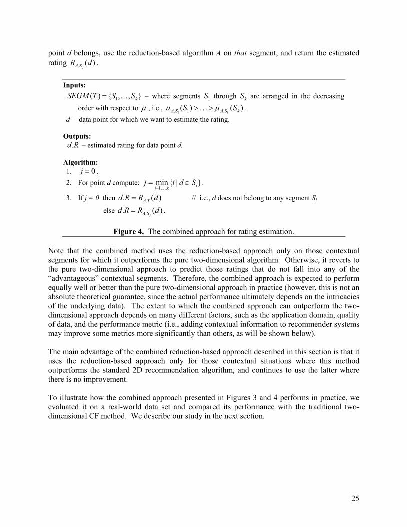
Figure 3. The algorithm for determining high-performing contextual segments. Finally, in Step 3 we also remove from ( )SEGM T those segments S, for which there exist strictly more general segment Q where the reduction-based approach performs better. It will also be seen from the rating estimation algorithm presented in Figure 4 that such underperforming segments will never be used for rating estimation purposes and, therefore, can be removed from ( )SEGM T . As a result, the algorithm produces the set of contextual segments ( )SEGM T on which the reduction-based algorithm A outperforms the pure algorithm A. Once we have the set of high-performance contextual segments ( )SEGM T , we can perform the second phase of the combined approach and determine which method to use in “real-time” when we need to produce an actual recommendation. The actual algorithm is presented in Figure 4. Given data point d for which we want to estimate the rating, we first go over the contextual segments 1( ) { , , }kSEGM T S S= … ordered in the decreasing order of their performance and select the best performing segment to which point d belongs. If d does not belong to any segment, we use the pure algorithm A (i.e., trained on the whole training data T) for rating prediction and return the estimated rating , ( )A TR d . Otherwise, we take the best-performing segment Sj to which

4 In practice, we use the term better to mean not only that , ,( ) ( )A S A TS Sµ µ> , but also that the difference between performances is substantial, e.g., it amounts to performing a statistical test that is dependent on the specific metric µ , as discussed in Section 5.

25

point d belongs, use the reduction-based algorithm A on that segment, and return the estimated rating , ( )

jA SR d .

Inputs:

1( ) { , , }kSEGM T S S= … – where segments 1S through kS are arranged in the decreasing order with respect to µ , i.e.,

1, 1 ,( ) ( )kA S A S kS Sµ µ> >… .

d – data point for which we want to estimate the rating.

Outputs: .d R – estimated rating for data point d.

Algorithm: 1. 0j = . 2. For point d compute:

1, ,min{ | }ii k

j i d S=

= ∈…

.

3. If j = 0 then ,. ( )A Td R R d= // i.e., d does not belong to any segment Si

else ,. ( )jA Sd R R d= .

Figure 4. The combined approach for rating estimation.

Note that the combined method uses the reduction-based approach only on those contextual segments for which it outperforms the pure two-dimensional algorithm. Otherwise, it reverts to the pure two-dimensional approach to predict those ratings that do not fall into any of the “advantageous” contextual segments. Therefore, the combined approach is expected to perform equally well or better than the pure two-dimensional approach in practice (however, this is not an absolute theoretical guarantee, since the actual performance ultimately depends on the intricacies of the underlying data). The extent to which the combined approach can outperform the two-dimensional approach depends on many different factors, such as the application domain, quality of data, and the performance metric (i.e., adding contextual information to recommender systems may improve some metrics more significantly than others, as will be shown below). The main advantage of the combined reduction-based approach described in this section is that it uses the reduction-based approach only for those contextual situations where this method outperforms the standard 2D recommendation algorithm, and continues to use the latter where there is no improvement. To illustrate how the combined approach presented in Figures 3 and 4 performs in practice, we evaluated it on a real-world data set and compared its performance with the traditional two-dimensional CF method. We describe our study in the next section.

26

5. Implementation and Evaluation of the Multidimensional Approach 5.1 Experimental Setup for a Multidimensional Movie Recommender System In order to compare the multidimensional recommendation approach to the traditional approaches, we decided to test our MD recommender system on a movie recommendation application. However, unlike traditional movie recommender systems, such as MovieLens [movielens.umn.edu], we wanted to take into consideration the contextual information about the viewing when recommending a movie, such as when the movie was seen, where, and with whom. Since such data was not available in any of the existing systems, we were not able to use any publicly available data. Instead, we built our own Web site and asked end-users to enter their ratings for movies they had seen, as well as the relevant contextual information. Our main goal was to compare the MD and 2D models and to show that the contextual information does matter, and, therefore, the extensive profiling and aggregation capabilities of the MD model were not required for this purpose. Therefore, our Web site had limited profiling and hierarchical aggregation capabilities. In particular, we built simple profiles and simple rating cubes that had built-in single-level hierarchies (e.g., a movie can be seen either in the movie theater or at home). As we will see below, this was sufficient for the purpose of comparing the MD and the 2D models. We set up our data collection Web site in such a way that users could select movies to rate either from memory or choose them from the list of all the available movies obtained from the Internet Movie Database site [imdb.com]. To help the users in the process of rating a movie, our data collection Web site also provided access to all the information about that movie at the Internet Movie Data Base. After users selected a movie to rate, they were prompted for the following information about the event of watching that movie, in addition to being asked to rate the movie:

• Time: when the movie was seen (choices: weekday, weekend, don’t remember); furthermore, if seen on a weekend, was it the opening weekend for the movie (choices: yes, no, don’t remember);

• Place: where the movie was seen (choices: in a movie theater, at home, don’t remember);

• Companion: with whom the movie was seen (choices: alone, with friends, with boyfriend/girlfriend, with family or others).

Therefore, we considered the contextual dimensions Time, Place, and Companion in addition to the traditional Person and Movie dimensions. Moreover, we decided to use “coarse granularity” for each of the contextual dimensions (e.g., partition the Time dimension only into weekend vs. weekday) for the following reasons. First, coarse granularities partitioned the data in a meaningful way from the consumer’s perspective. Second, having coarse granularities helped with the sparsity problem because they led to more data points per segment. Third, some of the ratings were for the movies that the users saw in the not-so-recent past and there was a tradeoff between recalling the specifics of the viewing context from memory and the accuracy of the data recalled.

27

Also, note that dimensions can have multiple aggregations that are overlapping, e.g., for dimension Time, we can have aggregations {weekdays, weekends} and {spring, summer, fall, winter}. In our case, based on our understanding of consumer behavior from pre-tests, we chose to use only one of these aggregations, i.e., {weekends, weekdays}. Participants rated the movies on a scale from 1 to 13, which is a more sensitive scale in comparison to the scales used in such applications as EachMovie, MovieLens and Amazon.com. The scale anchors were 1 (absolutely hated) and 13 (absolutely loved), and the midpoint was 7 (neither loved nor hated the movie). The scale was in the form of a drop down menu of rating choices with each point depicted numerically as well as graphically (i.e., showing the number of stars from 1 to 13) to ensure that it was well understood by subjects. The participants in our study were college students. Overall, 1755 ratings were entered by 117 students over a period of 12 months from May 2001 to April 2002. Since some students rated very few movies, we decided to drop those who had fewer than 10 movies for the purpose of our analysis. As a result, a few movies that were rated only by such students were also dropped. Therefore, from an initial list of 117 students and 210 movies, we finally had a list of 62 students, 202 movies and 1457 total ratings. Throughout the rest of the paper, we will use D to denote this set of 1457 ratings. As was pointed out in Section 3.1, it is important to understand which dimensions really matter in terms of making a “significant difference” in rating estimations. For example, perhaps the Time dimension does not really affect movie-watching experiences (i.e., perhaps it really does not matter whether you see a movie on a weekday or a weekend), and should be dropped from consideration and from the multidimensional cube of ratings. While designing our Web survey, we came up with the specific list of contextual dimensions by brainstorming amongst ourselves and coming up with the significant contextual dimensions and attributes, and then pre-testing these on students similar to those who would be participating in the survey. After the data had been collected, we tested each dimension to see if it significantly affected ratings using the ideas discussed in Section 3.1. This test is related to the problem of feature selection studied in data mining [Liu & Motoda 1998] and statistics [Chatterjee et al. 2000] because it determines which contextual dimensions matter for the rating estimation purposes and should be kept, and which dimensions could be dropped. In particular, we applied the following statistical test. For each dimension, we partitioned the ratings based on all the values (categories) of this dimension. For example, for the Time dimension, we partitioned all the ratings into either of the two categories, i.e., “weekend” or “weekday”. Then for each student5 we computed the average ratings for each category and applied a paired comparison t-test [Kachigan 1986] on the set of all users to determine whether there was a significant difference between the average ratings in these categories. For the binary dimensions Time, Place and OpeningWeekend the application of the paired t-test was straightforward and showed that the differences in ratings for the weekend/weekday, theater/home and opening/non-opening values were significant. Since the Companion dimension had 4 values, we applied the paired t-test to various pairs of values. From all these tests, we concluded that each of the contextual 5 We dropped those respondents who had not seen a certain minimum number of movies in each category (e.g., at least 3 movies on weekdays and weekends in our study).

28

dimensions affected ratings in a significant way and therefore should be kept for further considerations6. We implemented the algorithms described in Figures 3 and 4 (in Section 4) and tested them on the movie data described above. Before we provide the detailed description of the testing procedure and present the results, we first provide a broad overview of its major steps below.

1. We split the set of ratings D into 10 parts. Then we selected one part containing 10% of the

initial dataset (145 ratings) as evaluation dataset ( ED ) and the remaining 9 parts (or 90% of the data containing 1312 ratings) as modeling dataset ( MD ). The modeling dataset MD was used for the contextual segment selection purposes as described in Section 4. The evaluation dataset ED was used only to evaluate our recommendation approach for the real-time estimation of ratings (as described in Figure 4) and was not used in any contextual segment selection procedures described below. Based on our definitions, we have E MD D = ∅∩ and

E MD D D=∪ . 2. We ran our segment selection algorithm presented in Figure 3 on dataset MD . As a result,

we identified the segments on which the reduction-based approach significantly outperformed the standard CF method. The details of this step are presented in Section 5.2.

3. We evaluated the proposed combined recommendation approach by running the corresponding algorithm (i.e., from Figure 4) with the well-performing segments that were discovered in Step 2 (as described in the previous paragraph). In particular, we compared the performance of the combined approach to the performance of the standard CF using 10-fold cross-validation as follows. We took the 10 subsets of ratings produced in Step 1 and used them for the cross-validation purposes. In other words, we performed the evaluation procedure on 10 different 10%-90% splits of our initial dataset D into non-overlapping datasets ED and MD , where each time ED contained 145 ratings and constituted one of the 10 parts of D produced in Step 1, and MD contained 1312 ratings and constituted the remaining 9 parts of D. Moreover, all 10 evaluation datasets ED obtained during the 10-fold cross-validation process are pairwise non-overlapping. The details of this step are presented in Section 5.3.

We have used F-measure as the predictive performance measure µ (see Section 4.2), where a movie is considered to be “good” if it is rated above 10 (on a 13 point scale) and “bad” otherwise, and the precision and recall measures were defined in the standard way using these definitions of “good” and “bad.”

6 We would like to make the following observations pertaining to this test. First, it should be viewed only as a heuristic and not as the necessary or sufficient condition for the usefulness of the tested dimensions in a rigorous mathematical sense. Second, the t-test relies on the normality assumption of the underlying distribution. As an alternative, Wilcoxon test can be used for non-normal distributions [Kachigan 1986]. However, this test would still remain just another heuristic since, again, we cannot use it as a necessary or sufficient condition for the usefulness of the tested dimension in the reduction-based recommendation approach. Third, yet another method for eliminating some of the dimensions and features and, therefore, speeding up the process of identifying “good” segments would be to estimate multicollinearity [Kachigan 1986] among the features in various dimensions, and then drop some of the correlated features. However, we did not deploy this method in the project.

29

One caveat in the evaluation procedure outlined above is that we used only one 90%-10% split to select the set of segments on which the reduction-based approach significantly outperformed the standard CF method and used this same set of segments in the cross-validation procedure for the combined approach described in Step 3 above. Alternatively, we could have identified the set of outperforming segments each time when we did a fold in the 10-fold cross validation (e.g., did it inside the cross-validation loop). We followed the single-split approach for the following reasons. First, identification of outperforming segments (as described in Figure 3) is a computationally expensive process. Second, in any 10-fold cross-validation there is a significant training data overlap for each of the folds of the 10-fold cross validation, and, therefore, we do not expect to obtain a significantly different set of segments for different folds of cross-validation. For these reasons, we decided to use the same set of outperforming segments for each fold of cross-validation. 5.2 Selecting the Pertinent Segments: Evaluating the Reduction-Based Approach Although any available 2D recommendation algorithm A can be used in the combined approach (as described in Section 4.2 and presented in Figure 3), we decided to compare , ( )A S Sµ and

, ( )A T Sµ in terms of collaborative filtering (i.e., in both cases A is the same collaborative filtering method CF), since CF constitutes one of the most widely used tasks in recommender systems. For the purpose of our analysis, we have implemented one of the traditionally used versions of CF that computes the ratings using the adjusted weighted sum, as described in equation (5c) in Section 2. We used the cosine similarity measure (7) as the measure of similarity between users. As mentioned earlier, in this segment selection phase, we use dataset DM to find the most pertinent contextual segments for a given application. Initially, we ran the standard 2D CF method on dataset DM containing 1312 ratings using the bootstrapping method [Mitchell 1997, Hastie et al. 2001] with 500 random re-samples in order to obtain a baseline performance. In each re-sample, 29/30th of DM was used for training and the remaining 1/30th of DM for testing. More specifically, for each sample, we estimated ratings in the testing set of this sample using the ratings from the training set and did this operation 500 times. As a result, we obtained data set MX D⊆ , containing 1235 ratings ( 1235X = ), on which at least one rating from DM was tested. In other words, X represents a set of ratings that 2D CF was able to predict. Note, that in this particular case we have MX D⊂ (and not MX D= ), because CF was not able to predict all the ratings because of the sparsity-related limitations of the data. After that, we used equation (16) to compute average predicted ratings for all points in X. Then we used MAE, precision, recall and F-measures to determine the predictive performance of the standard CF method. We use precision and recall in the standard manner, i.e., precision is defined as the portion of truly “good” ratings among those that were predicted as “good” by the recommender system, and recall is defined as the portion of correctly predicted “good” ratings among all the ratings known to be “good”. Here we considered a movie to be “good” if its rating is higher than 10 (out of 13) and “bad” otherwise. F-measure is defined in a standard way [Baeza-Yates & Ribeiro-Neto 1999], i.e., as a harmonic mean of the precision and recall:

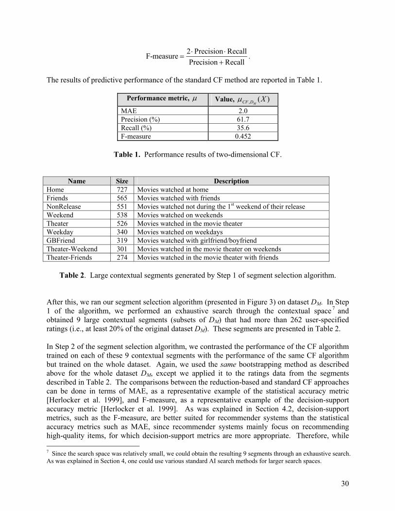
30

2 Precision RecallF-measurePrecision Recall⋅ ⋅

=+

.

The results of predictive performance of the standard CF method are reported in Table 1.

Performance metric, µ Value, , ( )MCF D Xµ

MAE 2.0 Precision (%) 61.7 Recall (%) 35.6 F-measure 0.452

Table 1. Performance results of two-dimensional CF.

Name Size Description Home 727 Movies watched at home Friends 565 Movies watched with friends NonRelease 551 Movies watched not during the 1st weekend of their release Weekend 538 Movies watched on weekends Theater 526 Movies watched in the movie theater Weekday 340 Movies watched on weekdays GBFriend 319 Movies watched with girlfriend/boyfriend Theater-Weekend 301 Movies watched in the movie theater on weekends Theater-Friends 274 Movies watched in the movie theater with friends

Table 2. Large contextual segments generated by Step 1 of segment selection algorithm. After this, we ran our segment selection algorithm (presented in Figure 3) on dataset DM. In Step 1 of the algorithm, we performed an exhaustive search through the contextual space 7 and obtained 9 large contextual segments (subsets of DM) that had more than 262 user-specified ratings (i.e., at least 20% of the original dataset DM). These segments are presented in Table 2. In Step 2 of the segment selection algorithm, we contrasted the performance of the CF algorithm trained on each of these 9 contextual segments with the performance of the same CF algorithm but trained on the whole dataset. Again, we used the same bootstrapping method as described above for the whole dataset DM, except we applied it to the ratings data from the segments described in Table 2. The comparisons between the reduction-based and standard CF approaches can be done in terms of MAE, as a representative example of the statistical accuracy metric [Herlocker et al. 1999], and F-measure, as a representative example of the decision-support accuracy metric [Herlocker et al. 1999]. As was explained in Section 4.2, decision-support metrics, such as the F-measure, are better suited for recommender systems than the statistical accuracy metrics such as MAE, since recommender systems mainly focus on recommending high-quality items, for which decision-support metrics are more appropriate. Therefore, while 7 Since the search space was relatively small, we could obtain the resulting 9 segments through an exhaustive search. As was explained in Section 4, one could use various standard AI search methods for larger search spaces.

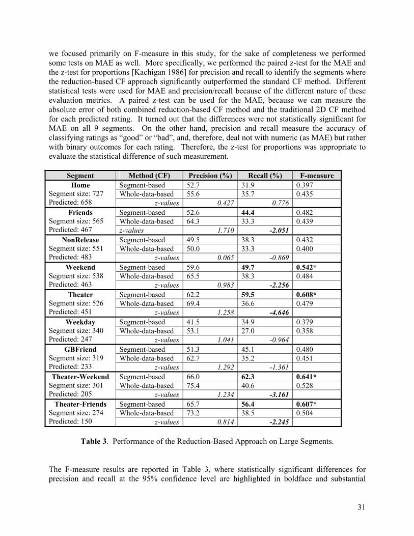
31

we focused primarily on F-measure in this study, for the sake of completeness we performed some tests on MAE as well. More specifically, we performed the paired z-test for the MAE and the z-test for proportions [Kachigan 1986] for precision and recall to identify the segments where the reduction-based CF approach significantly outperformed the standard CF method. Different statistical tests were used for MAE and precision/recall because of the different nature of these evaluation metrics. A paired z-test can be used for the MAE, because we can measure the absolute error of both combined reduction-based CF method and the traditional 2D CF method for each predicted rating. It turned out that the differences were not statistically significant for MAE on all 9 segments. On the other hand, precision and recall measure the accuracy of classifying ratings as “good” or “bad”, and, therefore, deal not with numeric (as MAE) but rather with binary outcomes for each rating. Therefore, the z-test for proportions was appropriate to evaluate the statistical difference of such measurement.

Segment Method (CF) Precision (%) Recall (%) F-measure Segment-based 52.7 31.9 0.397 Whole-data-based 55.6 35.7 0.435

Home Segment size: 727 Predicted: 658 z-values 0.427 0.776

Segment-based 52.6 44.4 0.482 Whole-data-based 64.3 33.3 0.439

Friends Segment size: 565 Predicted: 467 z-values 1.710 -2.051

Segment-based 49.5 38.3 0.432 Whole-data-based 50.0 33.3 0.400

NonRelease Segment size: 551 Predicted: 483 z-values 0.065 -0.869

Segment-based 59.6 49.7 0.542* Whole-data-based 65.5 38.3 0.484

Weekend Segment size: 538 Predicted: 463 z-values 0.983 -2.256

Segment-based 62.2 59.5 0.608* Whole-data-based 69.4 36.6 0.479

Theater Segment size: 526 Predicted: 451 z-values 1.258 -4.646

Segment-based 41.5 34.9 0.379 Whole-data-based 53.1 27.0 0.358

Weekday Segment size: 340 Predicted: 247 z-values 1.041 -0.964

Segment-based 51.3 45.1 0.480 Whole-data-based 62.7 35.2 0.451

GBFriend Segment size: 319 Predicted: 233 z-values 1.292 -1.361

Segment-based 66.0 62.3 0.641* Whole-data-based 75.4 40.6 0.528

Theater-Weekend Segment size: 301 Predicted: 205 z-values 1.234 -3.161

Segment-based 65.7 56.4 0.607* Whole-data-based 73.2 38.5 0.504

Theater-Friends Segment size: 274 Predicted: 150 z-values 0.814 -2.245

Table 3. Performance of the Reduction-Based Approach on Large Segments.

The F-measure results are reported in Table 3, where statistically significant differences for precision and recall at the 95% confidence level are highlighted in boldface and substantial

32

differences in F-measure are indicated in boldface and with symbol *. Note, that since there are no standard “substantial difference” definitions for the F-measure, for the purpose of this paper we considered the difference in F-measure as substantial if the actual difference in F-measures is more than 0.05 and the difference in at least one of its components (i.e., precision or recall) is statistically significant (determined using the z-test for proportions at the significance level 0.05). Also note that, since during this segment selection phase we compute the F-measure for each segment, the whole-data-based error rates are different for each segment. As mentioned in Section 4.2 (Figure 3), we evaluate each segment S by comparing how well the reduction-based CF approach predicts the ratings of this segment (i.e., we calculate , ( )A S Sµ ) with how well the standard 2D CF approach (i.e., the CF that is trained on the whole dataset) predicts the ratings of the same segment (i.e., we calculate , ( )A T Sµ ). Therefore, clearly, for different segments S, the whole-data-based error rate , ( )A T Sµ can be different. As Table 3 shows, the differences in F-measure turned out to be substantial on four segments out of 9, i.e., on these segments the reduction-based CF approach substantially outperformed the standard CF method in terms of the F-measure. These four segments are presented in Table 4 in the decreasing order, according to their F-measure.

Segment Segment-based F-measure Whole-data-based F-measure Theater-Weekend 0.641 0.528 Theater 0.608 0.479 Theater-Friends 0.607 0.504 Weekend 0.542 0.484

Table 4. Large contextual segments on which reduction-based approach substantially

outperformed the standard CF method in terms of the F-measure. In Step 3 of the segment selection algorithm, we identified the segments that passed the performance test in Step 2 and that also (a) were sub-segments of more general segments and (b) had worse performance results. In our case, the segment Theater-Friends (i.e., the ratings submitted by people who saw the movie in a movie theater with friends) was a subset of the Theater segment. Moreover, the Theater segment provided performance improvement in terms of the F-measure compared to the Theater-Friends segment. Therefore, using the segment selection algorithm, we discarded the smaller segment with a lower performance (i.e., Theater-Friends), and obtained the set

( ) { , , }SEGM T Theater -Weekend Theater Weekend= , which constituted the final result of the algorithm. Figure 5 provides graphical illustrations of Theater and Weekend segments within the cube of contextual dimensions, i.e., cube Companion×Place×Time.8 The Theater-Weekend segment is simply an intersection of these two segments.

8 We omitted User and Item dimensions in Figure 5 for the sake of the clarity of visualization.

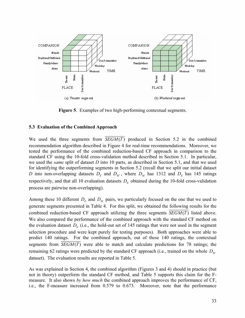
33

Figure 5. Examples of two high-performing contextual segments. 5.3 Evaluation of the Combined Approach We used the three segments from ( )SEGM T produced in Section 5.2 in the combined recommendation algorithm described in Figure 4 for real-time recommendations. Moreover, we tested the performance of the combined reduction-based CF approach in comparison to the standard CF using the 10-fold cross-validation method described in Section 5.1. In particular, we used the same split of dataset D into 10 parts, as described in Section 5.1, and that we used for identifying the outperforming segments in Section 5.2 (recall that we split our initial dataset D into non-overlapping datasets ED and MD , where MD has 1312 and ED has 145 ratings respectively, and that all 10 evaluation datasets ED obtained during the 10-fold cross-validation process are pairwise non-overlapping). Among these 10 different ED and MD pairs, we particularly focused on the one that we used to generate segments presented in Table 4. For this split, we obtained the following results for the combined reduction-based CF approach utilizing the three segments ( )SEGM T listed above. We also compared the performance of the combined approach with the standard CF method on the evaluation dataset ED (i.e., the hold-out set of 145 ratings that were not used in the segment selection procedure and were kept purely for testing purposes). Both approaches were able to predict 140 ratings. For the combined approach, out of these 140 ratings, the contextual segments from ( )SEGM T were able to match and calculate predictions for 78 ratings; the remaining 62 ratings were predicted by the standard CF approach (i.e., trained on the whole MD dataset). The evaluation results are reported in Table 5. As was explained in Section 4, the combined algorithm (Figures 3 and 4) should in practice (but not in theory) outperform the standard CF method, and Table 5 supports this claim for the F-measure. It also shows by how much the combined approach improves the performance of CF, i.e., the F-measure increased from 0.579 to 0.673. Moreover, note that the performance

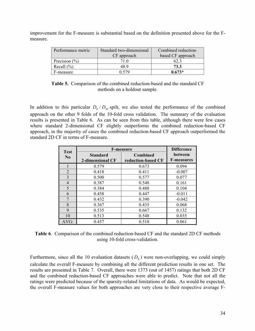
34

improvement for the F-measure is substantial based on the definition presented above for the F-measure.

Performance metric Standard two-dimensional CF approach

Combined reduction-based CF approach

Precision (%) 71.0 62.3 Recall (%) 48.9 73.3 F-measure 0.579 0.673*

Table 5. Comparison of the combined reduction-based and the standard CF

methods on a holdout sample. In addition to this particular ED / MD spilt, we also tested the performance of the combined approach on the other 9 folds of the 10-fold cross validation. The summary of the evaluation results is presented in Table 6. As can be seen from this table, although there were few cases where standard 2-dimensional CF slightly outperforms the combined reduction-based CF approach, in the majority of cases the combined reduction-based CF approach outperformed the standard 2D CF in terms of F-measure.

F-measure Test No Standard

2-dimensional CF Combined

reduction-based CF

Difference between

F-measures 1 0.579 0.673 0.094 2 0.418 0.411 -0.007 3 0.500 0.577 0.077 4 0.387 0.548 0.161 5 0.384 0.488 0.104 6 0.458 0.447 -0.011 7 0.432 0.390 -0.042 8 0.367 0.435 0.068 9 0.535 0.667 0.132

10 0.513 0.548 0.035 AVG: 0.457 0.518 0.061

Table 6. Comparison of the combined reduction-based CF and the standard 2D CF methods

using 10-fold cross-validation. Furthermore, since all the 10 evaluation datasets ( ED ) were non-overlapping, we could simply calculate the overall F-measure by combining all the different prediction results in one set. The results are presented in Table 7. Overall, there were 1373 (out of 1457) ratings that both 2D CF and the combined reduction-based CF approaches were able to predict. Note that not all the ratings were predicted because of the sparsity-related limitations of data. As would be expected, the overall F-measure values for both approaches are very close to their respective average F-

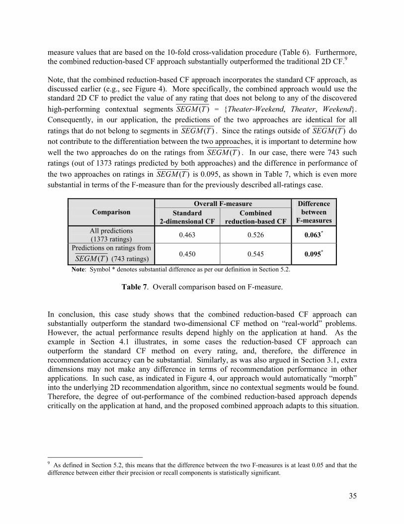
35

measure values that are based on the 10-fold cross-validation procedure (Table 6). Furthermore, the combined reduction-based CF approach substantially outperformed the traditional 2D CF.9 Note, that the combined reduction-based CF approach incorporates the standard CF approach, as discussed earlier (e.g., see Figure 4). More specifically, the combined approach would use the standard 2D CF to predict the value of any rating that does not belong to any of the discovered high-performing contextual segments ( )SEGM T = {Theater-Weekend, Theater, Weekend}. Consequently, in our application, the predictions of the two approaches are identical for all ratings that do not belong to segments in ( )SEGM T . Since the ratings outside of ( )SEGM T do not contribute to the differentiation between the two approaches, it is important to determine how well the two approaches do on the ratings from ( )SEGM T . In our case, there were 743 such ratings (out of 1373 ratings predicted by both approaches) and the difference in performance of the two approaches on ratings in ( )SEGM T is 0.095, as shown in Table 7, which is even more substantial in terms of the F-measure than for the previously described all-ratings case.

Overall F-measure Comparison Standard

2-dimensional CF Combined

reduction-based CF

Difference between

F-measures All predictions (1373 ratings) 0.463 0.526 0.063*

Predictions on ratings from ( )SEGM T (743 ratings) 0.450 0.545 0.095*

Note: Symbol * denotes substantial difference as per our definition in Section 5.2.

Table 7. Overall comparison based on F-measure. In conclusion, this case study shows that the combined reduction-based CF approach can substantially outperform the standard two-dimensional CF method on “real-world” problems. However, the actual performance results depend highly on the application at hand. As the example in Section 4.1 illustrates, in some cases the reduction-based CF approach can outperform the standard CF method on every rating, and, therefore, the difference in recommendation accuracy can be substantial. Similarly, as was also argued in Section 3.1, extra dimensions may not make any difference in terms of recommendation performance in other applications. In such case, as indicated in Figure 4, our approach would automatically “morph” into the underlying 2D recommendation algorithm, since no contextual segments would be found. Therefore, the degree of out-performance of the combined reduction-based approach depends critically on the application at hand, and the proposed combined approach adapts to this situation.

9 As defined in Section 5.2, this means that the difference between the two F-measures is at least 0.05 and that the difference between either their precision or recall components is statistically significant.

36

6. Conclusions and Future Work In this paper, we presented a multidimensional recommendation model that incorporates contextual information into the recommendation process and makes recommendations based on multiple dimensions, profiles, and aggregation hierarchies. We proposed the reduction-based approach for rating estimation that uses traditional collaborative filtering technique on contextual segments. We also demonstrated that in some situations context matters: multidimensional recommender systems can provide better recommendations in these situations by taking into the consideration additional contextual information. However, in most situations, contextual information provides better performance on some and worse performance on other segments. To address this problem, we proposed a combined reduction-based method and tested it using a standard two-dimensional collaborative filtering algorithm. We also demonstrated empirically that the combined reduction-based collaborative filtering approach substantially outperformed the standard 2D collaborative filtering method in terms of the F-measure. In the future, we plan to continue our work on the rating estimation problem. We plan to work on incorporating approaches other than the reduction-based into the recommendation methods. In particular, we plan to work on extending the model-based and heuristic-based approaches mentioned in Section 2 to the multidimensional setting. We also plan to work towards a better understanding of the pros and cons of the three rating estimation approaches, i.e., reduction-, heuristic- and model-based and on the comparative studies of these methods using different performance measures in addition to the F-measure used in our studies. We also plan to incorporate more advanced profiling methods mentioned in Section 3.2 into multi-dimensional recommendations. Furthermore, we plan to work on the general multilevel multidimensional rating estimation problem described at the beginning of Section 4 and explore further the relationship between recommender systems and OLAP technologies within the context of this problem. Finally, we plan to test our approach on other applications and additional data sets besides the movie rating data set described in this paper. References Adomavicius, G. and A. Tuzhilin, 2001. Multidimensional recommender systems: a data

warehousing approach. In Proceedings of the Second International Workshop on Electronic Commerce (WELCOM’01). Lecture Notes in Computer Science, vol. 2232, Springer.

Adomavicius, G. and A. Tuzhilin (2001b). Expert-driven validation of rule-based user models in personalization applications. Data Mining and Knowledge Discovery, 5(1/2):33-58, 2001.

Aggarwal, C. C., J. L. Wolf, K-L. Wu, and P. S. Yu, 1999. Horting hatches an egg: A new graph-theoretic approach to collaborative filtering. In Proceedings of the Fifth ACM SIGKDD International Conference on Knowledge Discovery and Data Mining.

Ansari, A., S. Essegaier, and R. Kohli, 2000. Internet recommendations systems. Journal of Marketing Research, pages 363-375.

Atkeson, C. G., Moore, A. W., and Schaal, S., 1997. Locally Weighted Learning. Artificial Intelligence Review, vol. 11, pp. 11-73.

Baeza-Yates, R. and B. Ribeiro-Neto, 1999. Modern Information Retrieval. Addison-Wesley. Balabanovic, M. and Y. Shoham, 1997. Fab: Content-based, collaborative recommendation.

Communications of the ACM, 40(3):66-72.

37

Basu, C., H. Hirsh, and W. Cohen, 1998. Recommendation as classification: Using social and content-based information in recommendation. In Recommender Systems. Papers from 1998 Workshop. Technical Report WS-98-08. AAAI Press.

Bettman, J. R., E. J. Johnson, and J. W. Payne, 1991. Consumer Decision Making. In Robertson and Kassarjian (Eds.), Handbook of Consumer Behavior, pp. 50-84. Prentice Hall.

Billsus, D. and M. Pazzani, 1998. Learning collaborative information filters. In International Conference on Machine Learning, Morgan Kaufmann Publishers.

Billsus, D. and M. Pazzani, 2000. User modeling for adaptive news access. User Modeling and User-Adapted Interaction, 10(2-3):147-180.

Breese, J. S., D. Heckerman, and C. Kadie, 1998. Empirical analysis of predictive algorithms for collaborative filtering. In Proceedings of the Fourteenth Conference on Uncertainty in Artificial Intelligence, Madison, WI.

Caglayan, A., M. Snorrason, J. Jacoby, J. Mazzu, R. Jones, and K. Kumar, 1997. Learn Sesame – a learning agent engine. Applied Artificial Intelligence, 11:393-412.

Chatterjee, S., A. S. Hadi, and B. Price, 2000. Regression Analysis by Example. John Wiley & Sons, Inc.

Chaudhuri, S. and U. Dayal, 1997. An overview of data warehousing and OLAP technology. ACM SIGMOD Record, 26(1):65-74.

Chien, Y-H. and E. I. George, 1999. A bayesian model for collaborative filtering. In Proceedings of the 7th International Workshop on Artificial Intelligence and Statistics.

Claypool, M., A. Gokhale, T. Miranda, P. Murnikov, D. Netes, and M. Sartin, 1999. Combining content-based and collaborative filters in an online newspaper. In ACM SIGIR'99. Workshop on Recommender Systems: Algorithms and Evaluation.

Condliff, M., D. Lewis, D. Madigan, and C. Posse, 1999. Bayesian mixed-effects models for recommender systems. In ACM SIGIR'99 Workshop on Recommender Systems: Algorithms and Evaluation.

Cortes, C., K. Fisher, D. Pregibon, A. Rogers, F. Smith, 2000. Hancock: a language for extracting signatures from data streams. In Proceedings of the Sixth ACM SIGKDD International Conference on Knowledge Discovery and Data Mining.

Delgado, J. and N. Ishii, 1999. Memory-based weighted-majority prediction for recommender systems. In ACM SIGIR'99 Workshop on Recommender Systems: Algorithms and Evaluation.

Duda, R. O., P. E. Hart, and D. G. Stork, 2001. Pattern Classification, John Wiley & Sons, Inc. Fan, J. and Li, R., 2003. Local Modeling: Density Estimation and Nonparametric Regression. In

Advanced Medical Statistics, J. Fang and Y. Lu (eds.), World Scientific, pp. 885-930. Getoor, L. and M. Sahami, 1999. Using probabilistic relational models for collaborative filtering.

In Workshop on Web Usage Analysis and User Profiling (WEBKDD'99). Goldberg, K., T. Roeder, D. Gupta, and C. Perkins, 2001. Eigentaste: A constant time

collaborative filtering algorithm. Information Retrieval Journal, 4(2):133-151. Han, J. and M. Kamber, 2001. Data Mining: Concepts and Techniques, Morgan Kaufmann. Hand, D., H. Mannila, and P. Smyth, 2001. Principles of Data Mining, MIT Press. Hastie, T., R. Tibshirani, and J. Friedman, 2001. The Elements of Statistical Learning, Springer. Herlocker, J. L. and J. A. Konstan, 2001. Content-Independent Task-Focused Recommendation.

IEEE Internet Computing, 5(6):40-47. Herlocker, J. L., J. A. Konstan, A. Borchers, and J. Riedl, 1999. An algorithmic framework for

performing collaborative filtering. In Proceedings of the 22nd Annual International ACM

38

SIGIR Conference on Research and Development in Information Retrieval (SIGIR’99), pp. 230 – 237.

Hill, W., L. Stead, M. Rosenstein, and G. Furnas, 1995. Recommending and evaluating choices in a virtual community of use. In Proceedings of CHI’95.

Kachigan, S. C. 1986. Statistical Analysis. Radius Press. Kimball, R., 1996. The Data Warehouse Toolkit. John Wiley & Sons, Inc. Klein, N. M. and M. Yadav, 1989. Context Effects on Effort and Accuracy in Choice: An

Inquiry into Adaptive Decision Making. Journal of Consumer Research, 16:410-420. Koller, D. and M. Sahami, 1996. Toward Optimal Feature Selection. In Proceedings of the

Thirteenth International Conference on Machine Learning, Morgan Kaufmann. Konstan, J. A., B. N. Miller, D. Maltz, J. L. Herlocker, L. R. Gordon, and J. Riedl, 1997.

GroupLens: Applying collaborative filtering to Usenet news. Communications of the ACM, 40(3):77-87.

Kotler, P. 2003. Marketing Management. 11th ed. Prentice Hall. Kumar, R., P. Raghavan, S. Rajagopalan, and A. Tomkins, 2001. Recommendation Systems: A

Probabilistic Analysis. Journal of Computer and System Sciences, 63(1):42-61. Lang, K., 1995. Newsweeder: Learning to filter netnews. In Proceedings of the 12th

International Conference on Machine Learning. Lee, W. S., 2001. Collaborative learning for recommender systems. In Proccedings of the

International Conference on Machine Learning. Lilien, G. L., P. Kotler, and S. K. Moorthy, 1992. Marketing Models, pp. 22-23. Prentice Hall. Liu, H. and H. Motoda, 1998. Feature Selection for Knowledge Discovery and Data Mining.

Kluwer Academic Publishers. Lussier, D. A. and R. W. Olshavsky, 1979. Task Complexity and Contingent Processing in

Brand Choice. Journal of Consumer Research, 6:154-165. Mitchell, T. M., 1997. Machine Learning, McGraw-Hill. Mobasher, B., H. Dai, T. Luo, Y. Sung, M. Nakagawa, and J. Wiltshire. Discovery of Aggregate

Usage Profiles for Web Personalization. In Proceedings of the Web Mining for E-Commerce Workshop (WebKDD’00), Boston, August 2000.

Mobasher, B., H. Dai, T. Luo, and M. Nakagawa. Using Sequential and Non-Sequential Patterns for Predictive Web Usage Mining Tasks. In Proceedings of the IEEE International Conference on Data Mining (ICDM’02), Maebashi City, Japan, December, 2002.

Mood, A. M., F. A. Graybill, and D. C. Boes, 1974. Introduction to the Theory of Statistics, 3rd ed., McGraw-Hill.

Mooney, R. J., P. N. Bennett, and L. Roy, 1998. Book recommending using text categorization with extracted information. In Recommender Systems. Papers from 1998 Workshop. Technical Report WS-98-08. AAAI Press.

Mooney, R. J., 1999. Content-based book recommending using learning for text categorization. In ACM SIGIR'99. Workshop on Recommender Systems: Algorithms and Evaluation.

Nakamura, A. and N. Abe, 1998. Collaborative filtering using weighted majority prediction algorithms. In Proceedings of the 15th International Conference on Machine Learning.

Oard, D. W. and J. Kim, 2001. Modeling information content using observable behavior. In Proceedings of the American Society for Information Science and Technology Conference, Washington, DC.

Pazzani, M., 1999. A framework for collaborative, content-based and demographic filtering. Artificial Intelligence Review, pages 393-408.

39

Pazzani, M. and D. Billsus, 1997. Learning and revising user profiles: The identification of interesting web sites. Machine Learning, 27:313-331.

Pennock, D. M. and E. Horvitz, 1999. Collaborative filtering by personality diagnosis: A hybrid memory- and model-based approach. In IJCAI'99 Workshop: Machine Learning for Information Filtering.

Ramakrishnan, R. and J. Gehrke, 2000. Database Management Systems. McGraw-Hill. Resnick, P., N. Iakovou, M. Sushak, P. Bergstrom, and J. Riedl, 1994. GroupLens: An open

architecture for collaborative filtering of netnews. In Proceedings of the 1994 Computer Supported Cooperative Work Conference.

Rossi, P. E., R. E. McCulloch, and G. M. Allenby, 1996. The Value of Purchase History in Target Marketing. Marketing Science, 15(4):321-340.

Salton, G., 1989. Automatic Text Processing. Addison-Wesley. Sarwar B., G. Karypis, J. Konstan, and J. Riedl, 2000. Application of dimensionality reduction

in recommender systems – a case study. In Proc. of the ACM WebKDD Workshop. Sarwar, B., G. Karypis, J. Konstan, and J. Riedl, 2001. Item-based Collaborative Filtering

Recommendation Algorithms. In Proc. of the 10th International WWW Conference. Shardanand, U. and P. Maes, 1995. Social information filtering: Algorithms for automating

‘word of mouth’. In Proceedings of the Conference on Human Factors in Computing Systems.

Soboroff, I. and C. Nicholas, 1999. Combining content and collaboration in text filtering. In IJCAI'99 Workshop: Machine Learning for Information Filtering.

Spiliopoulou, M., B. Mobasher, B. Berendt, and M. Nakagawa, 2003. A Framework for the Evaluation of Session Reconstruction Heuristics in Web Usage Analysis. INFORMS Journal of Computing, Special Issue on Mining Web-Based Data for E-Business Applications, 15(2).

Terveen, L., W. Hill, B. Amento, D. McDonald, and J. Creter, 1997. PHOAKS: A system for sharing recommendations. Communications of the ACM, 40(3):59-62.

Tran, T. and R. Cohen, 2000. Hybrid Recommender Systems for Electronic Commerce. In Knowledge-Based Electronic Markets, Papers from the AAAI Workshop, Technical Report WS-00-04, AAAI Press.

Ungar, L. H., and D. P. Foster, 1998. Clustering methods for collaborative filtering. In Recommender Systems. Papers from 1998 Workshop. Technical Report WS-98-08. AAAI Press.

Wade, W., 2003. A grocery cart that holds bread, butter and preferences. New York Times, Jan. 16.

Winston, P.H., 1992. Artificial Intelligence (3rd ed.). Addison-Wesley.

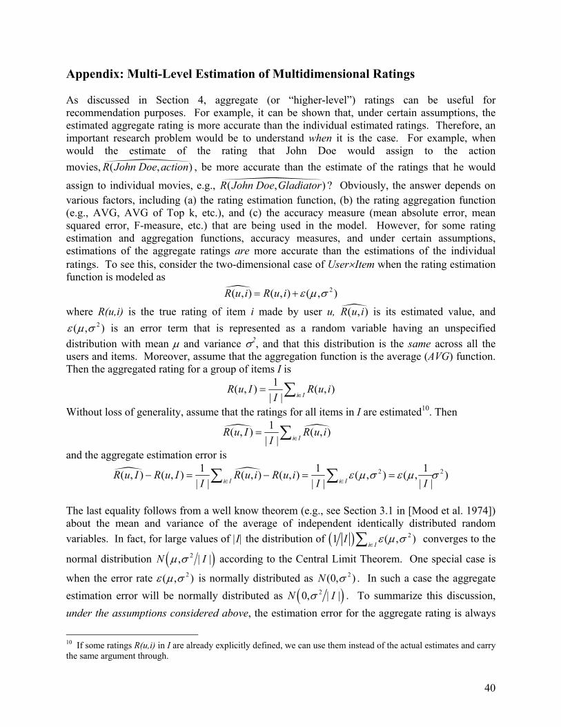
40

Appendix: Multi-Level Estimation of Multidimensional Ratings As discussed in Section 4, aggregate (or “higher-level”) ratings can be useful for recommendation purposes. For example, it can be shown that, under certain assumptions, the estimated aggregate rating is more accurate than the individual estimated ratings. Therefore, an important research problem would be to understand when it is the case. For example, when would the estimate of the rating that John Doe would assign to the action movies, ( , )R John Doe action , be more accurate than the estimate of the ratings that he would

assign to individual movies, e.g., ( , )R John Doe Gladiator ? Obviously, the answer depends on various factors, including (a) the rating estimation function, (b) the rating aggregation function (e.g., AVG, AVG of Top k, etc.), and (c) the accuracy measure (mean absolute error, mean squared error, F-measure, etc.) that are being used in the model. However, for some rating estimation and aggregation functions, accuracy measures, and under certain assumptions, estimations of the aggregate ratings are more accurate than the estimations of the individual ratings. To see this, consider the two-dimensional case of User×Item when the rating estimation function is modeled as 2( , ) ( , ) ( , )R u i R u i ε µ σ= +

where R(u,i) is the true rating of item i made by user u, ( , )R u i is its estimated value, and 2( , )ε µ σ is an error term that is represented as a random variable having an unspecified

distribution with mean µ and variance σ2, and that this distribution is the same across all the users and items. Moreover, assume that the aggregation function is the average (AVG) function. Then the aggregated rating for a group of items I is

1( , ) ( , )| | i I

R u I R u iI ∈

= ∑

Without loss of generality, assume that the ratings for all items in I are estimated10. Then

1( , ) ( , )| | i I

R u I R u iI ∈

= ∑

and the aggregate estimation error is 2 21 1 1( , ) ( , ) ( , ) ( , ) ( , ) ( , )

| | | | | |i I i IR u I R u I R u i R u i

I I Iε µ σ ε µ σ

∈ ∈− = − = =∑ ∑

The last equality follows from a well know theorem (e.g., see Section 3.1 in [Mood et al. 1974]) about the mean and variance of the average of independent identically distributed random variables. In fact, for large values of |I| the distribution of ( ) 21 ( , )

i II ε µ σ

∈∑ converges to the

normal distribution ( )2, | |N Iµ σ according to the Central Limit Theorem. One special case is

when the error rate 2( , )ε µ σ is normally distributed as 2(0, )N σ . In such a case the aggregate estimation error will be normally distributed as ( )20, | |N Iσ . To summarize this discussion, under the assumptions considered above, the estimation error for the aggregate rating is always

10 If some ratings R(u,i) in I are already explicitly defined, we can use them instead of the actual estimates and carry the same argument through.

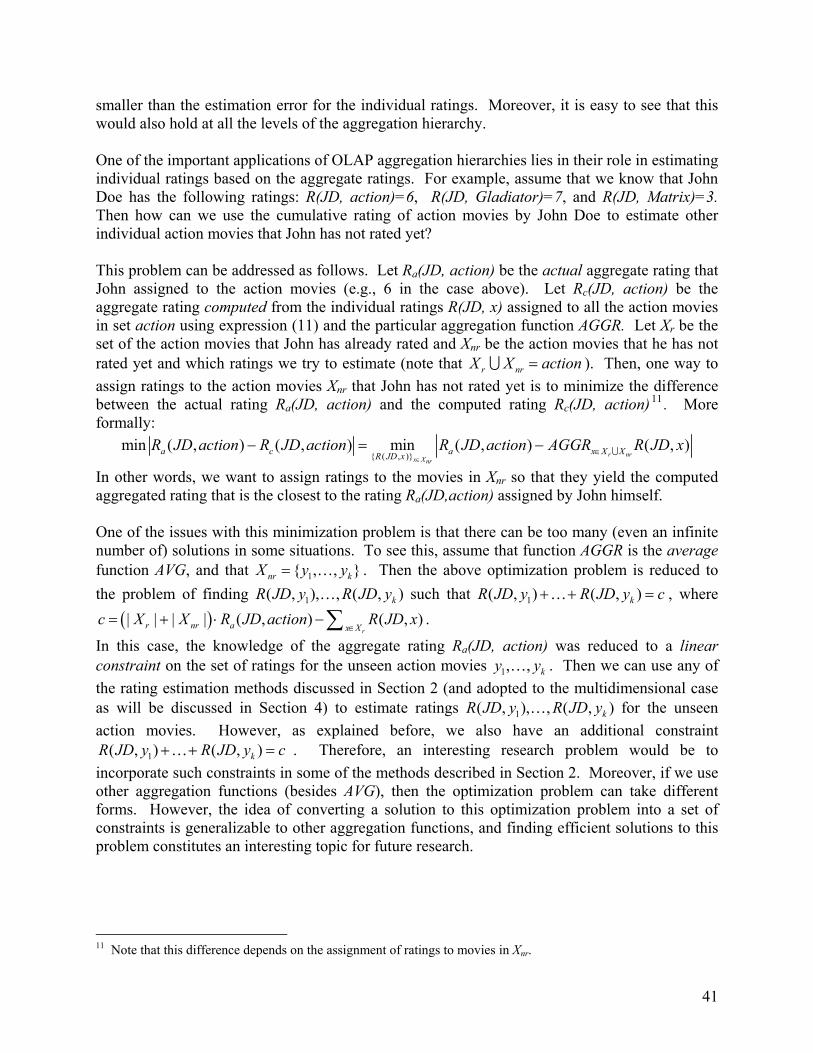
41

smaller than the estimation error for the individual ratings. Moreover, it is easy to see that this would also hold at all the levels of the aggregation hierarchy. One of the important applications of OLAP aggregation hierarchies lies in their role in estimating individual ratings based on the aggregate ratings. For example, assume that we know that John Doe has the following ratings: R(JD, action)=6, R(JD, Gladiator)=7, and R(JD, Matrix)=3. Then how can we use the cumulative rating of action movies by John Doe to estimate other individual action movies that John has not rated yet? This problem can be addressed as follows. Let Ra(JD, action) be the actual aggregate rating that John assigned to the action movies (e.g., 6 in the case above). Let Rc(JD, action) be the aggregate rating computed from the individual ratings R(JD, x) assigned to all the action movies in set action using expression (11) and the particular aggregation function AGGR. Let Xr be the set of the action movies that John has already rated and Xnr be the action movies that he has not rated yet and which ratings we try to estimate (note that r nrX X action=∪ ). Then, one way to assign ratings to the action movies Xnr that John has not rated yet is to minimize the difference between the actual rating Ra(JD, action) and the computed rating Rc(JD, action)11 . More formally:

{ ( , )}min ( , ) ( , ) min ( , ) ( , )

r nrx Xnr

a c a x X XR JD xR JD action R JD action R JD action AGGR R JD x

∈∈− = − ∪

In other words, we want to assign ratings to the movies in Xnr so that they yield the computed aggregated rating that is the closest to the rating Ra(JD,action) assigned by John himself. One of the issues with this minimization problem is that there can be too many (even an infinite number of) solutions in some situations. To see this, assume that function AGGR is the average function AVG, and that 1{ , , }nr kX y y= … . Then the above optimization problem is reduced to the problem of finding 1( , ), , ( , )kR JD y R JD y… such that 1( , ) ( , )kR JD y R JD y c+ + =… , where

( )| | | | ( , ) ( , )r

r nr a x Xc X X R JD action R JD x

∈= + ⋅ − ∑ .

In this case, the knowledge of the aggregate rating Ra(JD, action) was reduced to a linear constraint on the set of ratings for the unseen action movies 1, , ky y… . Then we can use any of the rating estimation methods discussed in Section 2 (and adopted to the multidimensional case as will be discussed in Section 4) to estimate ratings 1( , ), , ( , )kR JD y R JD y… for the unseen action movies. However, as explained before, we also have an additional constraint

1( , ) ( , )kR JD y R JD y c+ + =… . Therefore, an interesting research problem would be to incorporate such constraints in some of the methods described in Section 2. Moreover, if we use other aggregation functions (besides AVG), then the optimization problem can take different forms. However, the idea of converting a solution to this optimization problem into a set of constraints is generalizable to other aggregation functions, and finding efficient solutions to this problem constitutes an interesting topic for future research.

11 Note that this difference depends on the assignment of ratings to movies in Xnr.