1

Income Taxes: Policy Issues

Can Model Income Tax as Tax on Wage Income

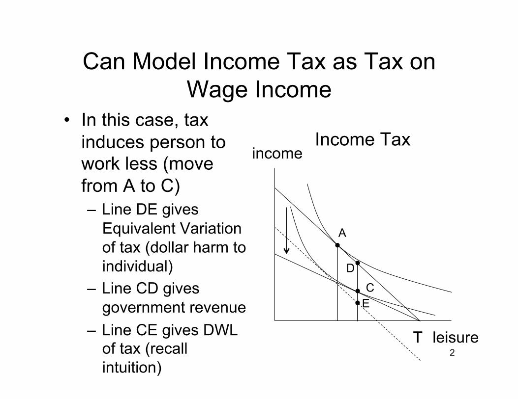
•  In this case, tax induces person to work less (move from A to C) –  Line DE gives

Equivalent Variation of tax (dollar harm to individual)

–  Line CD gives government revenue

–  Line CE gives DWL of tax (recall intuition)

Income Tax

2 T leisure

income

A

C

D

E

DWL from tax on wages

•  As an exercise, illustrate the Equivalent Variation, Government Revenue, and DWL of a wage tax for the two other cases – One where hours remain unchanged – One where hours increase

3

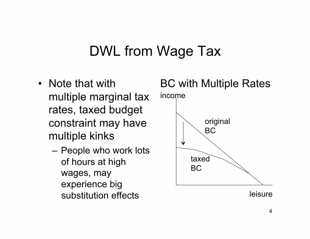
DWL from Wage Tax

•  Note that with multiple marginal tax rates, taxed budget constraint may have multiple kinks –  People who work lots

of hours at high wages, may experience big substitution effects

BC with Multiple Rates

4

leisure

income

original BC

taxed BC

Should Family Income or Individual Income be Taxed?

•  In the last set of notes we analyzed income taxation with rising marginal tax rates, assuming each person was single. But lots of people live in multi-person households. – Should taxation take this into account? – Canadian tax system does not tax people

differently based on marital status – Should households with the same family

income pay the same amount of taxes? 5

Family vs. Individual Taxation

6

•  How is personal income treated within marriage? –  Most OECD countries - including Canada - have

adopted individual taxation: a married individual is treated no differently from a single individual for tax purposes.

–  In contrast, countries such as the US, Ireland and Germany apply personal income tax schedules that depend on marital status (in Canadian policy debates this is referred to as “income-splitting”)

“Income Splitting” is an Example of Family Taxation

•  Income splitting assesses a (common law) spouse’s tax liability by attributing half of the taxable income of the couple to each spouse. – This often allows the high earning spouse

to be taxed at a lower marginal tax rate on their last dollars earned.

7

Policy Debate: Canada •  Calls for income splitting in Canada

increased in October 2006 when government announced income splitting for seniors.

•  Harper has now (2014) placed this front and center as a key campaign platform.

•  According to a poll 70% of Canadians support income splitting. – As we will see later, many probably don’t

understand the full implications 8

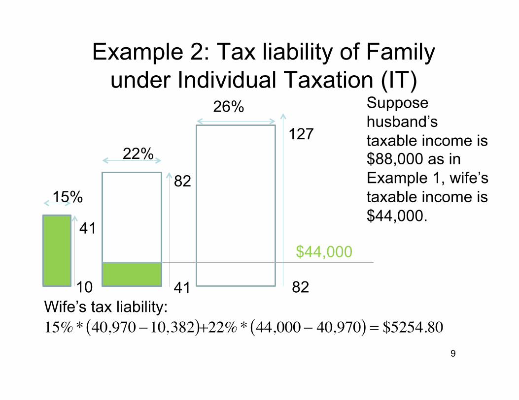
Example 2: Tax liability of Family under Individual Taxation (IT)

9

Suppose husband’s taxable income is $88,000 as in Example 1, wife’s taxable income is $44,000.

Wife’s tax liability:

82

41

22%

$44,000

�

+22%* 44,000 − 40,970( ) = $5254.80

�

15%* 40,970 −10,382( )

10

41

15%

82

26%

127

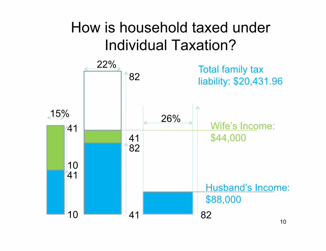
How is household taxed under Individual Taxation?

10 10

82

41 82

Husband’s Income:$88,000

41

26%

82

41

22%

Wife’s Income:$44,000

10

41

15%

Total family tax liability: $20,431.96

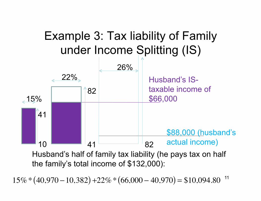
Example 3: Tax liability of Family under Income Splitting (IS)

11

$88,000 (husband’s actual income) 10

Husband’s half of family tax liability (he pays tax on half the family’s total income of $132,000):

82

41

22%

82

Husband’s IS-taxable income of $66,000

�

+22%* 66,000 − 40,970( ) = $10,094.80

41

15%

26%

�

15%* 40,970 −10,382( )

12

10

82

41

22%

82

wife’s IS-taxable income of $66,000

41

15%

26%

�

15%* 40,970 −10,382( )

$44,000 (wife’s actual income)

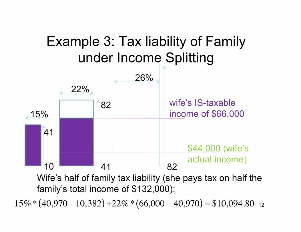
Example 3: Tax liability of Family under Income Splitting

Wife’s half of family tax liability (she pays tax on half the family’s total income of $132,000):

�

+22%* 66,000 − 40,970( ) = $10,094.80

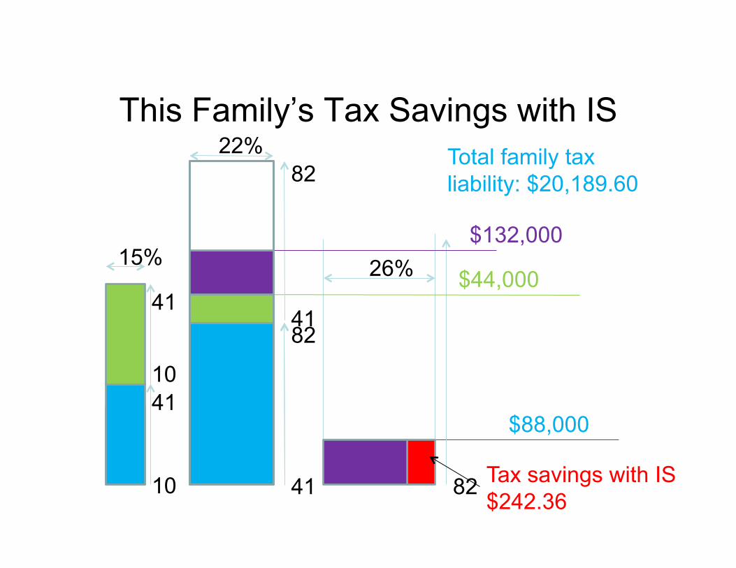
This Family’s Tax Savings with IS

10

82

41 82

$88,000

41

26%

82

41

22%

$44,000

10

41

15%

Tax savings with IS $242.36

$132,000

Total family tax liability: $20,189.60

Family’s Tax Savings under Income Splitting

14

The way IS saves the family money on taxes is that it allows the husband to transfer some of his income taxed at 26% (under individual taxation) to his wife; who is only taxed at 22% (under individual taxation) on her last dollar earned

The family saves $242.36 under IS. This is because the last $6059 of the husband’s income is taxed at 22% rather than 26%. $6059*0.04=$242.36.

In general, tax economists refer to shifting income from a higher tax bracket to a lower tax bracket as “tax arbitrage”. IS is an example of tax arbitrage.

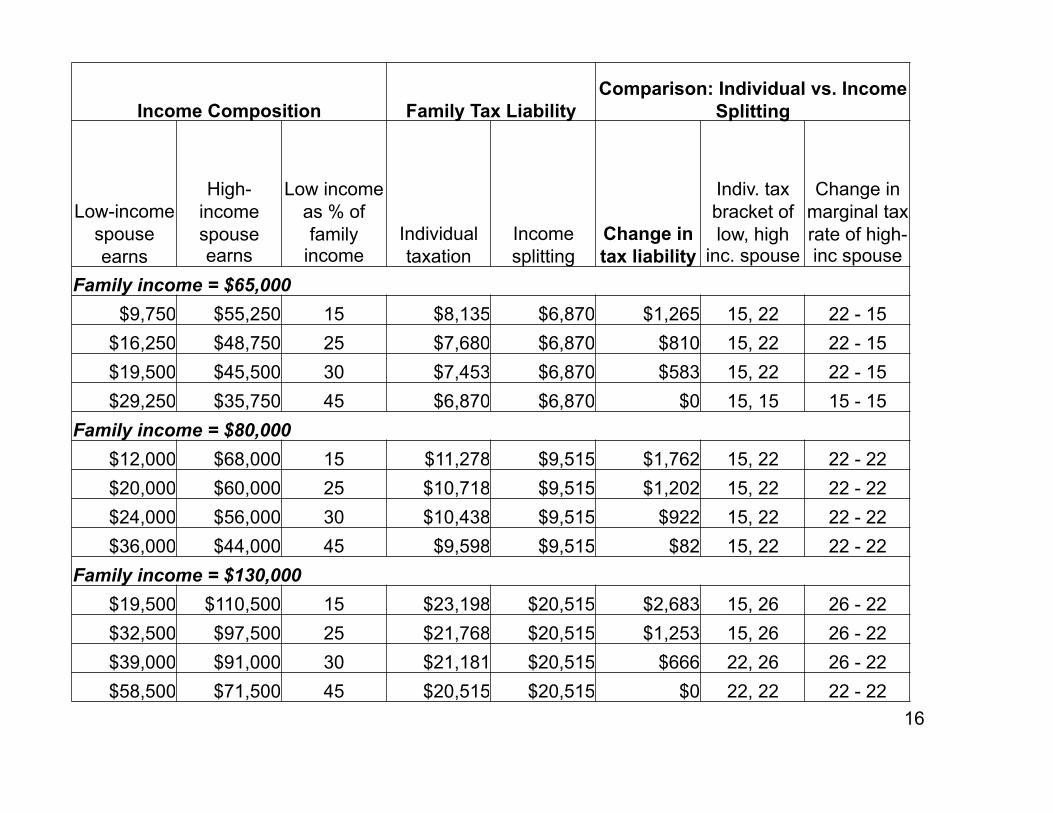
How Does Income Splitting Affect Tax Liabilities for Different Households?

15

Depends on 1) Total household income (families with higher income tend to benefit more) 2) Distribution of income within household (families where one person makes a lot more than their spouse benefit more)

Note: Next slide is example using older tax rates (not 2010 rates, as has been used in the examples up until now). This is from a paper by Professor Gugl.

Basic story would be similar applying more current rates.

16

Income Composition Family Tax Liability Comparison: Individual vs. Income

Splitting

Low-income spouse earns

High-income spouse earns

Low income as % of family

income Individual taxation

Income splitting

Change in tax liability

Indiv. tax bracket of low, high

inc. spouse

Change in marginal tax rate of high-inc spouse

Family income = $65,000 $9,750 $55,250 15 $8,135 $6,870 $1,265 15, 22 22 - 15

$16,250 $48,750 25 $7,680 $6,870 $810 15, 22 22 - 15 $19,500 $45,500 30 $7,453 $6,870 $583 15, 22 22 - 15 $29,250 $35,750 45 $6,870 $6,870 $0 15, 15 15 - 15

Family income = $80,000 $12,000 $68,000 15 $11,278 $9,515 $1,762 15, 22 22 - 22 $20,000 $60,000 25 $10,718 $9,515 $1,202 15, 22 22 - 22 $24,000 $56,000 30 $10,438 $9,515 $922 15, 22 22 - 22 $36,000 $44,000 45 $9,598 $9,515 $82 15, 22 22 - 22

Family income = $130,000 $19,500 $110,500 15 $23,198 $20,515 $2,683 15, 26 26 - 22 $32,500 $97,500 25 $21,768 $20,515 $1,253 15, 26 26 - 22 $39,000 $91,000 30 $21,181 $20,515 $666 22, 26 26 - 22 $58,500 $71,500 45 $20,515 $20,515 $0 22, 22 22 - 22

Individual Taxation vs. Income Splitting—Which Way Should

Canada Go? •  Let’s consider the question from both an

equity and efficiency point of view •  Equity first:

–  Consider 2 households that make $100,000 a year.

•  Assume both households have 2 kids •  In one, husband works and wife doesn’t (wife stays home

and looks after the kids). Husband makes $100,000 •  In other, both work and both make $50,000. Put kids in

daycare.

17

Income Splitting--Equity •  Under individual taxation, household with

stay-at-home wife pays more taxes than household where both work –  Is this fair? –  The ability-to-pay principle says that households

with more resources should pay more –  On surface, both households have same

resources ($100k in income); suggests income splitting would be fairer (because both households would pay same taxes)—but look a bit deeper

18

Income Splitting--Equity •  Household with stay-at-home wife has access

to wife’s home production capabilities; wife in other household works, so her ability to contribute to household production is lower –  Because the 1-income household can produce its

own daycare (by the stay-at-home spouse), it produces additional resources (beyond the $100k income) compared with the 2-income household

–  Therefore, the 1-income household arguably has a greater ability to pay than the 1-income household—so perhaps individual taxation (which has them pay more in taxes than the 2-income household) is actually fairer than IS

19

Income Splitting--Equity •  On the other hand, consider a single mother

who makes $100,000 vs. a couple where the wife makes $100,000 and the husband stays home with the kids (under IS this family pays less taxes; under IT both families pay same) – Do both households have the same ability

to pay (ATP)? •  Claim: Couple have higher ATP

–  Produce more total resource due to home childcare – Can share resource costs (like car, kitchen, etc.)

across 2 people, while single mom can’t

•  Claim: Single mom has higher ATP –  Fewer mouths to feed (no husband)

20

Income Splitting--Equity

•  Under individual taxation, both families would be taxed the same amount

•  Under income splitting, couple would pay less taxes than the single-mom – Depending on your view of ability to pay for

the two households, this may or may not seem fair

21

Income Splitting--Efficiency •  Arguably income splitting subsidizes home

production (by giving biggest tax benefits to couples who have one person specialize in home production) –  Home production is already untaxed, which means

a pre-existing distortion is present •  Childcare you buy is taxed (the labour is taxed and there

are consumption taxes on childcare services); hiring tradespeople to do home repairs is taxed (both labour and consumption); so doing these things yourself (i.e. failing to specialize) helps you avoid paying those taxes

•  Yet, economists argue specialization and gains from trade should be pursued for efficiency

•  IS makes this distortion worse by increasing the tax benefit to doing your own homecare, doing your own home repairs, etc.

22

Income Splitting--Efficiency

•  Another problem with IS is that it raises the marginal tax rate on the secondary earner in a couple –  Under IT a stay-at-home spouse faces a 0% tax

rate on her first dollar earned –  Under IS, the same person faces whatever tax

rate applies to half of her spouse’s income –  This may deter secondary earners from entering

the labour force or increasing their hours worked

23

Income Splitting--Efficiency •  Flip side of this is that IS lowers the MTR on

the primary earner –  Other things held constant, lowering the high MTR

of one spouse and raising the low MTR of the other spouse would likely be efficiency enhancing

–  Why? Because, ceteris paribus, substitution effects are likely to be very large with high MTRs and small with low MTRs; under fairly standard assumptions, DWL increases at an increasing rate as MTRs increase. So lowering high MTRs by a bit while increasing low MTRs by a bit would, ceteris paribus, lower DWL

24

Income Splitting--Efficiency •  Problem is the ceteris paribus assumption on

previous slide is probably wrong •  Secondary earners likely have very different

labour supply behaviour than primary earners •  For example: married men are thought to have

much less wage elastic labour supply than married women (econometric studies suggest this) –  If that’s because married men have a smaller

substitution effect response to wage changes than married women, this means we can reduce DWL by taxing married men more than we tax married women

–  IT (the current system in Canada does this); IS would get rid of that differential taxation—this could actually be bad for efficiency (i.e. it could increase DWL)

25

Income Splitting—One more point on Equity

•  Men still make more than women in Canada, so women tend to be secondary earners –  IS tends to promote specialization between the

spouses (i.e. promotes having 1 primary earner and 1 stay at home spouse)

–  Staying home with the kids lowers your ability to earn money in the marketplace

•  Human capital depreciates over time •  Staying at home forgoes workplace experience that

would have boosted your wage

–  So women who stay at home with the kids tend to lose financial independence 26

Income Splitting—One more point on Equity

•  The ability to work has done a lot for women’s rights –  Women can leave lousy marriages more easily if

they can get a good job and support themselves –  Women who can leave a marriage tend to have

greater rights within that marriage—greater bargaining power

–  IS essentially rewards families that keep the wife at home—in doing so it may erode women’s bargaining power within marriage and leave them more economically vulnerable in the event that their marriage breaks up

27

Note: IS is not revenue neutral

•  Note that if we switch to income splitting (Harper has proposed this) while holding marginal tax rates (and brackets) constant, government revenues will fall –  Because some families pay less taxes under IS,

while others pay same taxes •  In order to implement IS in revenue neutral

way, tax rates would have to rise –  Means some couples would pay more taxes under

IS; and single people would pay more taxes under IS.

28

The Income Tax and Saving

•  Another policy question about income taxes is what income should be taxed? – Some argue interest and capital income

should not be taxed – Yet the people who make the most interest

and capital income tend to be very rich, hence exempting such income is seen by many as unfair

– Why wouldn’t we want to tax interest income? Because it may distort saving decisions 29

30

Modeling Saving

•  Decisions about whether to consume income today or consume it tomorrow (i.e. save) can be modeled just like a choice between goods x and y –  Our two goods are “consumption today” and

“consumption tomorrow” –  By giving up a dollar of consumption today, one

can receive (1+r) of consumption tomorrow (r is interest rate)

–  Can think of this using indifference curves and budget constraint

31

Saving Decision •  Let w1 be endowment (income) in period 1; c1 be

consumption in period 1 •  Let w2 be endowment (income) in period 2; c2 be

consumption in period 2 •  Budget Constraint (assuming person lives 2 periods) Consumption in period 2: c2 c2=(w1-c1)(1+r)+w2 In other words in period 2, I can consume as much as I

saved from period 1, (w1-c1), plus the interest on that saving, (w1-c1)r plus whatever I earn in period 2.

•  Rearranging gives c1+ c2/(1+r)=w1+w2/(1+r), in other words

PV(Consumption)= PV(Income) PV: present discounted value

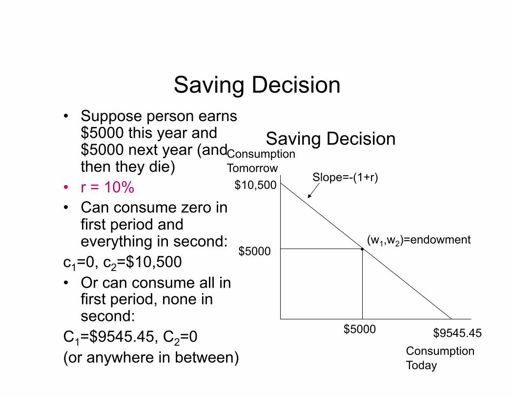
Saving Decision •  Suppose person earns

$5000 this year and $5000 next year (and then they die)

•  r = 10% •  Can consume zero in

first period and everything in second:

c1=0, c2=$10,500 •  Or can consume all in

first period, none in second:

C1=$9545.45, C2=0 (or anywhere in between)

Saving Decision

Consumption Today

Consumption Tomorrow

$5000

$5000

Slope=-(1+r)

$9545.45

$10,500

• (w1,w2)=endowment

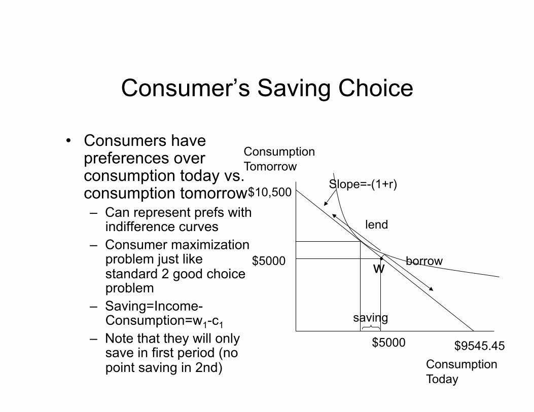
Consumer’s Saving Choice

•  Consumers have preferences over consumption today vs. consumption tomorrow –  Can represent prefs with

indifference curves –  Consumer maximization

problem just like standard 2 good choice problem

–  Saving=Income-Consumption=w1-c1

–  Note that they will only save in first period (no point saving in 2nd)

Consumption Tomorrow

$5000

$5000

Slope=-(1+r)

$9545.45

$10,500

Consumption Today

borrow

lend

saving

• w

34

Taxing Saving

•  A tax on saving has the same effect as lowering the interest rate; will change budget constraint. –  Assume no credit constraints –  Assume borrowing interest rate is same as saving

(lending) interest rate –  Imagine government imposes a tax of t on interest

income •  Affects slope of budget constraint to left of endowment

point

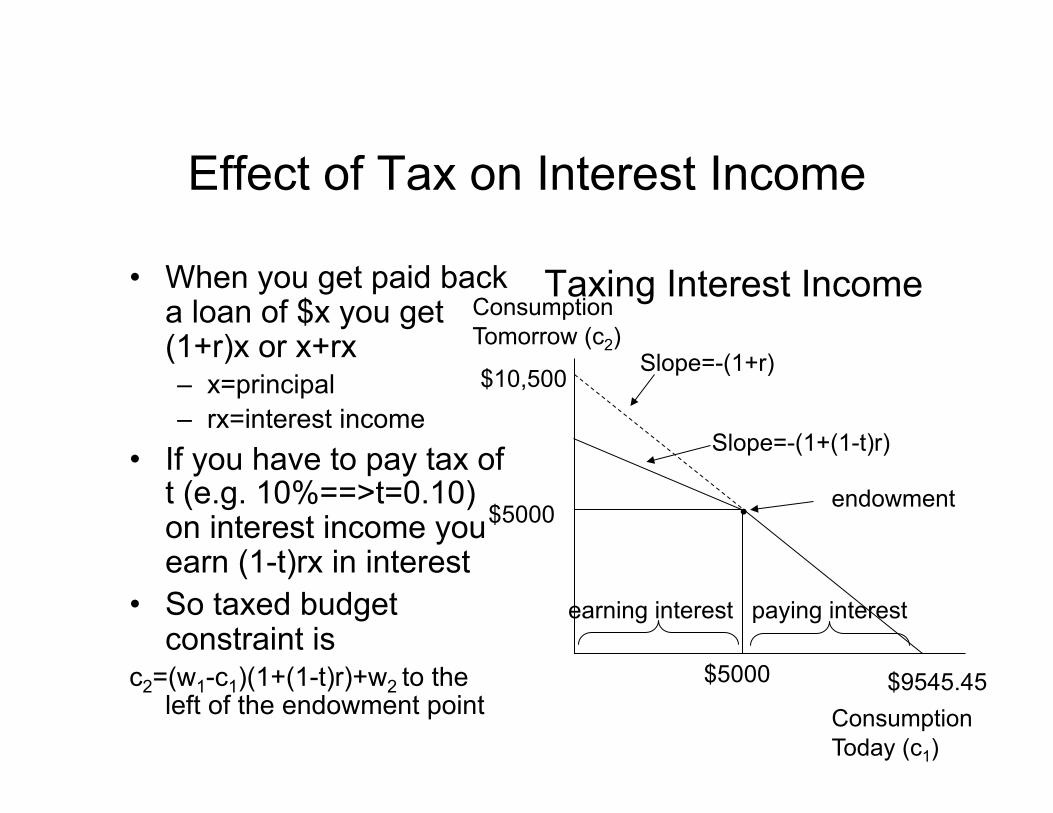
Effect of Tax on Interest Income

•  When you get paid back a loan of $x you get (1+r)x or x+rx –  x=principal –  rx=interest income

•  If you have to pay tax of t (e.g. 10%==>t=0.10) on interest income you earn (1-t)rx in interest

•  So taxed budget constraint is

c2=(w1-c1)(1+(1-t)r)+w2 to the left of the endowment point

Taxing Interest Income Consumption Tomorrow (c2)

$5000

$5000

Slope=-(1+r)

$9545.45

$10,500

Consumption Today (c1)

Slope=-(1+(1-t)r)

paying interest earning interest

endowment •

36

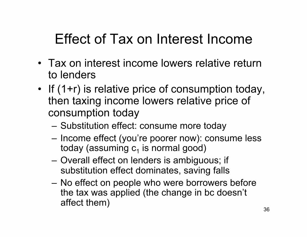
Effect of Tax on Interest Income •  Tax on interest income lowers relative return

to lenders •  If (1+r) is relative price of consumption today,

then taxing income lowers relative price of consumption today –  Substitution effect: consume more today –  Income effect (you’re poorer now): consume less

today (assuming c1 is normal good) –  Overall effect on lenders is ambiguous; if

substitution effect dominates, saving falls –  No effect on people who were borrowers before

the tax was applied (the change in bc doesn’t affect them)

37

Tax on Interest Income (with deductibility of interest payments)

•  In some cases, interest payments are tax deductible –  Interest payments on Student Loans in Canada –  Business interest payments in Canada and US

•  This causes whole budget constraint to pivot around the endowment point, reflecting the fact that borrowing becomes cheaper as a result of the deductibility of interest income

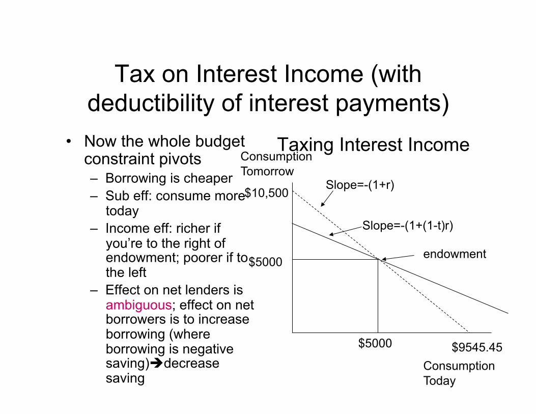
Tax on Interest Income (with deductibility of interest payments)

•  Now the whole budget constraint pivots –  Borrowing is cheaper –  Sub eff: consume more

today –  Income eff: richer if

you’re to the right of endowment; poorer if to the left

–  Effect on net lenders is ambiguous; effect on net borrowers is to increase borrowing (where borrowing is negative saving)decrease saving

Taxing Interest Income Consumption Tomorrow

$5000

$5000

Slope=-(1+r)

$9545.45

$10,500

Consumption Today

Slope=-(1+(1-t)r)

endowment

Taxing Interest Income Distorts Saving

•  Because taxing interest income may distort saving decisions many economists favour consumption taxes – Many conservatives were unhappy with

Harper’s reduction of the GST from 7% to 5%

– We’ll discuss consumption taxes more in the next set of notes

39

40

Effect of Tax on Interest Income on National Saving

•  Note that when economists are interested in policies to boost saving, what they really want to increase is national saving (government plus personal plus business saving –  The previous analysis only covers the effect of a

tax on interest income on personal saving –  If government used these taxes on interest income

to lower budget deficits, they could increase national saving, even if they decreased personal saving in the process.

41

Effect of Tax on Interest Income: Empirical Evidence

•  Just as an empirical literature explores the effect of wages on hours worked, there is one exploring effect of interest rates on saving –  Boskin (US, 1978) finds the elasticity of saving wrt

net real interest rate is between 0.2 and 0.4 •  In other words, a 10% increase in the real interest rate

boosts saving by 2-4% •  Suggests that taxes on saving (e.g. the income tax)

lower saving –  Auerbach and Slemrod (1997) find that income

and substitution effects roughly cancel each other out (using US data)

42

Effect of Tax on Interest Income: Empirical Evidence

•  Beach, Boadway, Bruce (1988) find little effect of taxes on interest income on Canadian saving overall

•  RRSPs and RPPs present an interesting policy case –  Tax deductible retirement savings plans and

retirement pension plans –  Means that you can subtract amount of income put

in RRSP/RPP from your gross income –  Meant to promote personal saving –  Tax deductible contributions limited to $7500 in

1987; up to around $16,000 today. Do these raise saving?

43

Effect of Tax on Interest Income: Empirical Evidence

•  Empirical evidence on RRSPs, etc. is mixed –  Carrol and Summers (1987), Engelhardt (1996),

Beach, Boadway, and Bruce (1988) find that programs like these boost saving

–  Morissette and Drolet (2001) say it’s unclear; Milligan finds marginal tax rates have small effect on participation in RRSPs

–  Engen, Gale, and Scholz claim such programs in US have little effect; while others (Poterba, Venti, and Wise and others) find evidence that such programs boost saving

–  Remember, though, that giving tax breaks reduces govt saving, so relevant question is whether these programs boost overall saving!

44

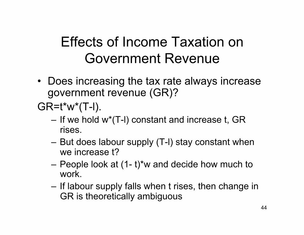
Effects of Income Taxation on Government Revenue

•  Does increasing the tax rate always increase government revenue (GR)?

GR=t*w*(T-l). –  If we hold w*(T-l) constant and increase t, GR

rises. –  But does labour supply (T-l) stay constant when

we increase t? –  People look at (1- t)*w and decide how much to

work. –  If labour supply falls when t rises, then change in

GR is theoretically ambiguous

45

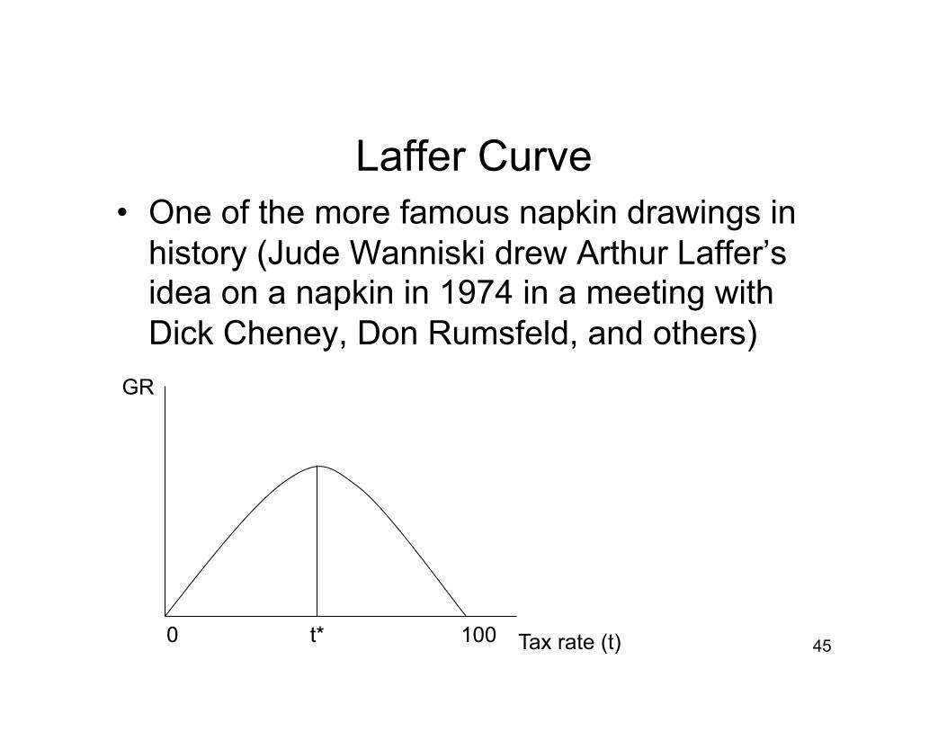
Laffer Curve •  One of the more famous napkin drawings in

history (Jude Wanniski drew Arthur Laffer’s idea on a napkin in 1974 in a meeting with Dick Cheney, Don Rumsfeld, and others)

GR

Tax rate (t) t* 0 100

46

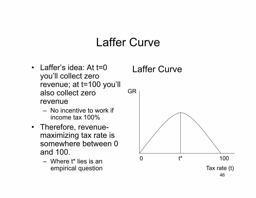
Laffer Curve

•  Laffer’s idea: At t=0 you’ll collect zero revenue; at t=100 you’ll also collect zero revenue –  No incentive to work if

income tax 100% •  Therefore, revenue-

maximizing tax rate is somewhere between 0 and 100. –  Where t* lies is an

empirical question

Laffer Curve

GR

Tax rate (t)

t* 0 100

47

Are we above or below t*? –  When Reagan took power, he cut taxes and

revenue from personal income tax fell by 9% from 1980-1984, even though average income rose by 4% during the same period. This suggests that US was to the left of t* when Reagan came into office (oops!)

–  Bush II tried the same thing: again revenues fell –  In 1980s average Swede paid a top marginal tax

rate of 80%. Studies have suggested that Sweden would have raised its tax revenues if it had cut its tax rates (they may have been to the right of t*)

–  Note that the intuition behind the Laffer Curve is relevant to other forms of taxation—not just income taxes