Generational War on Inflation: Optimal Inflation Rates for ...

INCOME-SPECIFIC INFLATION RATES AND THE EFFECTS OF MONETARY POLICY: THE CASE OF NORTH
MACEDONIA
Biljana Jovanovic
Marko Josimovski
November, 2020

Table of contents
Introduction
Literature review
Data
Stylized facts
Empirical analysis
Conclusion and recommendations for future research

Introduction
Research topic: The distributional effects of monetary policy onthe consumer price indices (CPIs) specific for households whichbelong to different income groups
Distributional consequences of macroeconomic policies – a relativelynew phenomenon in academic research (originates from fiscalpolicy incidence analysis in high-income countries)
Several theoretical channels through which monetary policy mightaffect income and consumption inequality (income compositionchannel, portfolio channel, financial segmentation channel, savingsredistribution channel)
Conventional and unconventional tools
We investigate primarily the transimission mechanism proposed byCravino et al. (2018)

Literature review
Previous literature suggests that inflation is in fact heterogeneous,hence different socio-economic and demographic groups experiencedifferent levels of inflation (high vs. low-income people, young vs.elderly people, more educated vs. less educated people, borrowersvs. savers, etc.)
Attempts for different measures of inflation for separate socio-economic groups, such as the elderly people (Amble and Stewart,1994) and low-income people (Garner et al., 1996)
Recent literature related to the distributional consequences ofmonetary policy argues that monetary policy decisions can result indifferent effects among different groups of economic agents(Auclert, 2017)

Literature review
Cravino et al. (2018) find that following a monetary policy shock,inflation rates specific for high-income households react lesscompared to the inflation rates specific for middle-incomehouseholds. This happens because of two reasons:
the effect of monetary shock on prices is heterogeneous across types of goods and services
consumption baskets differ across the income distribution.
Data
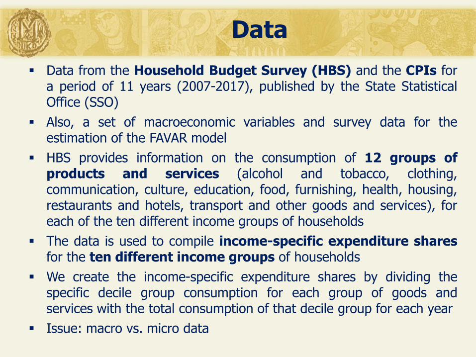
Data from the Household Budget Survey (HBS) and the CPIs fora period of 11 years (2007-2017), published by the State StatisticalOffice (SSO)
Also, a set of macroeconomic variables and survey data for theestimation of the FAVAR model
HBS provides information on the consumption of 12 groups ofproducts and services (alcohol and tobacco, clothing,communication, culture, education, food, furnishing, health, housing,restaurants and hotels, transport and other goods and services), foreach of the ten different income groups of households
The data is used to compile income-specific expenditure sharesfor the ten different income groups of households
We create the income-specific expenditure shares by dividing thespecific decile group consumption for each group of goods andservices with the total consumption of that decile group for each year
Issue: macro vs. micro data

Stylized facts
Figure 1: Expenditure shares over household income deciles, 2007
Figure 2: Expenditure shares over household income deciles, 2017
(Source: State statistical data and authors’ own calculations)
Expenditure shares are relatively stable throughout the years
The expenditure share of food decreases as income rises, while the sharesof other categories tend to increase (housing, transport, health, clothing)
Stylized facts
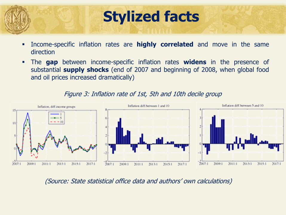
Figure 3: Inflation rate of 1st, 5th and 10th decile group
(Source: State statistical office data and authors’ own calculations)
Income-specific inflation rates are highly correlated and move in the samedirection
The gap between income-specific inflation rates widens in the presence ofsubstantial supply shocks (end of 2007 and beginning of 2008, when global foodand oil prices increased dramatically)

Stylized facts
Income-specific weighted frequency of price changes for a specific year is calculated as:
ҧ𝜃ℎ =
𝑖=1
𝑛
𝑤𝑖ℎ𝜃𝑖
ҧ𝜃ℎ is the income-specific frequency of price changes, 𝑤𝑖ℎ is the
income-specific expenditure share for each group of products and services, 𝜃𝑖 is the frequency of price changes
We rely on Aucremanne and Dhyne (2004) who calculate frequencies of price changes for the Belgium economy

Stylized facts
Figure 4: Weighted frequency of price changes, average for the period 2007-2017
Figure 5: Standard deviation of the changes in the consumption price indices
(Source: State statistical office data and authors’ own calculations)
Lower and middle-income households have higher frequency of price changes andhigher standard deviation of changes in the CPIs, relative to high-incomehouseholds

Empirical analysis – FAVAR model
FAVAR model (Bernanke, Boivin, and Eliasz , 2005 – BBE and Boivin,Giannoni, and Mihov, 2009)
vector Xt = income specific price indices, as well as theadditional variables: sector-level producer price indices, sector-level industrial production, labour market indicators, credit andmonetary indicators, external sector indicators, economic sentimentindicators and other relevant variables.
monthly data; period 2007m1-2017m12
all variables are seasonally adjusted and transformed in order toachieve stationarity
all information variables are classified in two groups - slow-movingand fast moving variables same as in BBE (2005)
Empirical analysis – FAVAR model
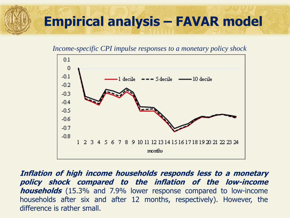
Inflation of high income households responds less to a monetarypolicy shock compared to the inflation of the low-incomehouseholds (15.3% and 7.9% lower response compared to low-incomehouseholds after six and after 12 months, respectively). However, thedifference is rather small.
Income-specific CPI impulse responses to a monetary policy shock

Empirical analysis – Small scale model simulations
Small scale gap model that reflects the structure of the Macedonianeconomy (simplified version of MAKPAM model)
𝜋𝑡ℎ = 𝛼1
𝜋𝑡+1 ∙ 𝜋𝑡+1 + 𝛼1𝜋𝑡−1 ∙ 𝜋𝑡−1 + 𝛼1
𝜋𝑡𝑜𝑖𝑙
∙ 𝜋𝑡𝑜𝑖𝑙 + (1− 𝛼1
𝜋𝑡+1 − 𝛼1𝜋𝑡−1 − 𝛼1
𝜋𝑡𝑜𝑖𝑙
) ∙ 𝜋𝑡𝑒𝑓+ 𝛼1
𝑦𝑔𝑎𝑝∙ 𝑦𝑔𝑎𝑝𝑡 + 𝜀𝑡
𝜋𝑡
𝜋𝑡𝑇𝑂𝑇 = 𝑠ℎ𝜋𝑡
ℎ
ℎ
𝑦𝑔𝑎𝑝𝑡 = 𝛼2𝑦𝑔𝑎𝑝 𝑡−1 ∙ 𝑦𝑔𝑎𝑝𝑡−1 + 𝛼2
𝑞𝑔𝑎𝑝 𝑡−1 ∙ 𝑞𝑔𝑎𝑝𝑡−1 + 𝛼2𝑟𝑔𝑎𝑝 𝑡−1 ∙ 𝑟𝑔𝑎𝑝𝑡−1 + 𝛼2
𝑦𝑓𝑔𝑎𝑝 𝑡−1 ∙ 𝑦𝑓𝑔𝑎𝑝𝑡−1 + 𝜀𝑡𝑦𝑔𝑎𝑝 𝑡
Phillips curves
IS curve

Empirical analysis – Small scale model simulations
Monetary policy
𝑖𝑡 = 𝑖𝑠𝑡𝑎𝑟 𝑡+ 𝑟𝑖𝑠𝑘𝑝𝑟𝑒𝑚𝑖𝑢𝑚 + 𝜀𝑡
𝑖
𝑟𝑖𝑠𝑘𝑝𝑟𝑒𝑚𝑖𝑢𝑚 = 𝑟𝑖𝑠𝑘𝑝𝑟𝑒𝑚𝑆𝑆 + 𝑟𝑖𝑠𝑘𝑝𝑟𝑒𝑚
𝑟𝑠𝑟𝑔𝑎𝑝
𝑟𝑖𝑠𝑘𝑝𝑟𝑒𝑚𝑟𝑠𝑟𝑔𝑎𝑝 = 𝛼3
𝑟𝑖𝑠𝑘𝑝𝑟𝑒𝑚∙ 𝑟𝑠𝑟𝑔𝑎𝑝𝑡+4
𝑟𝑠𝑟𝑔𝑎𝑝𝑡 = 𝛼4𝑟𝑠𝑟𝑔𝑎𝑝 𝑡−1 ∙ 𝑟𝑠𝑟𝑔𝑎𝑝𝑡−1 + 1 − 𝛼4
𝑟𝑠𝑟𝑔𝑎𝑝 𝑡−1
∙ 𝛼4𝑖𝑛𝑓
∙ 𝜋𝑡𝑇𝑂𝑇 − 𝜋𝑡
𝑒𝑓 + 𝛼4
𝑑𝑒𝑚𝑎𝑛𝑑 ∙ 𝛼4𝑦𝑔𝑎𝑝 𝑡−1 ∙ 𝑦𝑔𝑎𝑝𝑡−1 − 1 − 𝛼4
𝑦𝑔𝑎𝑝 𝑡−1 ∗ 𝑦𝑓𝑔𝑎𝑝𝑡−1
+ 𝜀𝑡𝑟𝑠𝑟𝑔𝑎𝑝 𝑡

Empirical analysis – Small scale model simulations
To evaluate the distributional effects of monetary policy threescenarios were created:
• baseline scenario, where the monetary policy reaction is driven by themodel structure and the assumptions of the exogenous variables (foreigninflation, foreign demand, oil prices and foreign interest rate)
• two alternative scenarios, in both of which we assume that monetaryauthorities decided to change interest rates because of some additionalfactor not anticipated in the model
• the interest rate in the two-year period ahead is higher incomparison to the baseline (assumes that the interest rate will hoveraround 6%)
• the interest rate in the two-year period ahead is lower in comparisonto the baseline (assumes that the interest rate will hover around0.5%)

Empirical analysis – Small scale model simulations
• Monetary policy has a higher impact on the lower-income groups
• However, the impact is relatively small regardless of the income group.
Impulse responses of household-specific CPIs to a monetary shock

Empirical analysis – Small scale model simulations
• Monetary policy has a higher impact (in both directions) on the lower-incomegroups
• However, the impact is relatively small regardless of the income group.
Difference in the inflation rates under different scenarios for the lowest and the highest-income decile group (in percentage points)

Conclusion and recommendations for future research
• Different income groups have different consumption baskets – lower-incomehouseholds spend more for food relative to higher-income households.
• Income-specific inflation rates tend to diverge significantly in the presence ofsubstantial supply shocks.
• Lower-income households are characterized with more flexible and morevolatile prices relative to the prices of higher-income households.
• As the distributional impact of monetary policy is concerned, both the impulseresponse analysis and the model simulation exercise indicate that theresponse of lower-income households’ inflation rate is higher incomparison to higher-income households, meaning that changes in thepolicy rate affect more the households on the left side of the incomedistribution line.
• However, given that the difference in the response between the incomegroups is relatively small, we can conclude that, in general the monetarypolicy in the Macedonian case does not exhibit asymmetrical effecton different income groups of households.

Conclusion and recommendations for future research
Recommendations for future research:
• Conducting the analysis by using the HBS micro data -disaggregated analysis on income-specific inflation rates, with aspecial focus on certain percentiles such as the top 1%, where asignificant part of the income and wealth is concentrated.
• Modification of the modelling framework - DSGE model willallow to model income-specific price stickiness more consistently,model extension with different IS curves which will describe thebehavior of the income variables for different households. Thismodification will be helpful in studying the direct impact of monetarypolicy stance on income distribution, as well as its distributionalconsequences.

Thank you!