
Income Satisfaction Inequality and its Causesftp.iza.org/dp854.pdf · Income Satisfaction...
29
IZA DP No. 854 Income Satisfaction Inequality and its Causes Ada Ferrer-i-Carbonell Bernard M. S. Van Praag DISCUSSION PAPER SERIES Forschungsinstitut zur Zukunft der Arbeit Institute for the Study of Labor August 2003
Transcript of Income Satisfaction Inequality and its Causesftp.iza.org/dp854.pdf · Income Satisfaction...

IZA DP No. 854
Income Satisfaction Inequality and its Causes
Ada Ferrer-i-CarbonellBernard M. S. Van Praag
DI
SC
US
SI
ON
PA
PE
R S
ER
IE
S
Forschungsinstitutzur Zukunft der ArbeitInstitute for the Studyof Labor
August 2003

Income Satisfaction Inequality
and its Causes
Ada Ferrer-i-Carbonell AIAS, University of Amsterdam
Bernard M. S. Van Praag University of Amsterdam, Tinbergen Institute
and IZA Bonn
Discussion Paper No. 854 August 2003
IZA
P.O. Box 7240 D-53072 Bonn
Germany
Tel.: +49-228-3894-0 Fax: +49-228-3894-210
Email: [email protected]
This Discussion Paper is issued within the framework of IZA’s research area Welfare State and Labor Market. Any opinions expressed here are those of the author(s) and not those of the institute. Research disseminated by IZA may include views on policy, but the institute itself takes no institutional policy positions. The Institute for the Study of Labor (IZA) in Bonn is a local and virtual international research center and a place of communication between science, politics and business. IZA is an independent, nonprofit limited liability company (Gesellschaft mit beschränkter Haftung) supported by Deutsche Post World Net. The center is associated with the University of Bonn and offers a stimulating research environment through its research networks, research support, and visitors and doctoral programs. IZA engages in (i) original and internationally competitive research in all fields of labor economics, (ii) development of policy concepts, and (iii) dissemination of research results and concepts to the interested public. The current research program deals with (1) mobility and flexibility of labor, (2) internationalization of labor markets, (3) welfare state and labor market, (4) labor markets in transition countries, (5) the future of labor, (6) evaluation of labor market policies and projects and (7) general labor economics. IZA Discussion Papers often represent preliminary work and are circulated to encourage discussion. Citation of such a paper should account for its provisional character. A revised version may be available on the IZA website (www.iza.org) or directly from the author.

IZA Discussion Paper No. 854 August 2003
ABSTRACT
Income Satisfaction Inequality and its Causes∗
In this paper, the concept of Income Satisfaction Inequality is operationalized on the basis of individual responses to an Income Satisfaction question posed in the German Socio-Economic Panel (GSOEP). Income satisfaction is the subjective analogue of the objective income concept and includes objective income inequality as a special case. The paper introduces a method to decompose Income Satisfaction Inequality according to the contributions from variables such as income, education, and the number of children. Given the panel structure of the data, inequality may be attributed partly to permanent individual circumstances and partly to transitory changes. The paper shows that by far the largest part of the satisfaction inequality has to be ascribed to unobserved heterogeneity. Distinguishing between a structural and an unexplained part of inequality we find that income explains the largest part of structural Income Satisfaction Inequality together with household membership; for non-working individuals, the age distribution is very relevant as well. JEL Classification: D63, I32 Keywords: equivalent income, financial satisfaction, income satisfaction, income
inequality, variance decomposition Corresponding author: Bernard M.S. van Praag Faculty of Economics and Econometrics University of Amsterdam Roetersstraat 11 1018 WB Amsterdam The Netherlands Tel.: +31 20 525 60 18 Fax: +31 20 525 60 13 Email: [email protected]
∗ The authors would like to thank Peter Hop and Adam Booij for their help and comments. The usual disclaimers apply.

1
1. Introduction
Since Gini (1912) and Dalton (1920), the distribution and inequality of income has
been an important subject of study for economic and social scientists. Recent surveys
are offered in the handbooks edited by Atkinson and Bourguignon (1999) and Silber
(1999). The study of income inequality entails two main issues (see Cowell (1999)).
First, the income concept has to be operationalized and measured. Second, a definition
of inequality has to be agreed upon and consequently an index of inequality, namely a
measure of the dispersion of income or welfare, has to be chosen.
The basic question underneath is why we are so interested in income inequality.
It is not just an administrative statistic. The reason is that income or ‘equivalent
income’ is taken as a proxy for welfare. It follows that income inequality is seen as
synonymous to welfare inequality, a performance index of society. The literature
bears witness that there is no generally accepted measure of welfare. This is caused
among other reasons by uneasiness about whether income in itself is a suitable
measure of welfare. This is especially true for modern welfare states where a
considerable part of our consumption is provided by the state and not through the
market. Additionally, income has to be corrected for individual and household
characteristics if it aims at measuring welfare. For example, it is evident that two
households with the same income but different family sizes fs will need different
incomes to be equally satisfied. Hence, income y should be ‘corrected’ for family size,
which would lead to what is known as ‘equivalent income’ y� . For instance, if we
apply the correction factor g(fs) equivalent income becomes . ( )y y g fs=� . In order to
compare incomes and to get some idea about income inequality, it does not make
much sense to define income inequality on nominal income. Inequality should be
measured with respect to equivalent incomes. It is evident that this will change
income inequality. For instance, if we use the variance of log-incomes as inequality
measure, we have
var(ln( )) var(ln( )) var(ln( ( )) 2cov(ln( ), ln( ( )))y y g fs y g fs= + +� (1)
This shows that the inequality of equivalent incomes, as defined by the log-variance,
will differ from the inequality of nominal incomes. One may be larger or smaller than

2
the other. It is evident that there are more intervening variables than family size. Say,
we have a vector x of such variables. Then the definition of equivalent income may be
straightforwardly generalized to correct for x. The problem is the definition and
empirical operationalization of the correction factor g(x). Our definition will be
simple. If two individuals A and B report to be equally satisfied with their incomes yA
and yB , we assume those two incomes to be equivalent. This implies that if we take A
as the reference then ( ) B Ag x y y= . In practice, this factor is derived by looking at
’income satisfaction questions’, which are now posed as a matter of routine in socio-
economic surveys. It may also be that x includes some unobservable individual
characteristics ε . Then exact correction at the individual level will be impossible.
However, we can still operationalize for those variables that are observable.
In this paper, we try a new approach to assess inequality by not looking at
nominal income as our basic variable but at the satisfaction derived from income. We
call this income satisfaction and we measure it by means of individual answers to an
income satisfaction question. We believe that this empirical approach leads to a
welfare inequality concept, which does more right to our intuitive feelings about
inequality than the measures that account for income differences only.
It is possible to define and measure an index for income satisfaction. The
income satisfaction concept used in this paper does implicitly incorporate the
necessary corrections. Income satisfaction is empirically defined through the analysis
of individual responses to an income satisfaction question. The paper aims at
explaining the individual’ s income satisfaction by objective variables x, such as
income, education, and number of individuals in the household. We denote that
satisfaction by ( ; , )f y x θ , where y stands for nominal income, x for other individual
circumstances, and θ for a vector of parameters to be estimated. If there
holds ( ; , )f y x yθ ≡ , the subjective perception will coincide with nominal income.
Hence, usual income inequality is embedded in the income satisfaction inequality
concept as a special case.
The income satisfaction inequality (Isat) is here measured in such a way that if
satisfaction would coincide with income, that is yxyf ≡),;( θ , then (Isat) would equal
the variance of log-incomes. The variance of the logarithm is one of the most
frequently used measures of inequality, together with the relative mean deviation, the
3
variance, the coefficient of variation, the Atkinson index, the Gini coefficient, and
Theil’ s entropy measure (see Atkinson, 1970; Sen, 1973). All those inequality
measures are functions of moments of the income distribution. It is well known that
the distribution of personal and household incomes is rather well –approximated by a
log- normal distribution. When the income distribution is (approximately) log-normal
),( 2σµΛ , all income inequality indexes are (approximately) functions of the two
distribution parameters. The parameter µ gives the position of the distribution, while
2σ is a measure for the relative income differences. The log-variance ( 2σ ) as a
measure of inequality has the advantage that it does not depend on the money unit.
Other measures are simple functions of 2σ and µ . Theil (1967, chapter 4; 1979)
shows that the Theil Entropy measure equals (½) 2σ in the case of log-normality. Van
Praag (1978) derived a similar result for the Atkinson index, and Aitchison and
Brown (1960) for the Gini index. If approximate log-normality holds, there is not
much to be gained by considering more indices simultaneously, given the one-to-one
relationship between such indexes. Thus we will exclusively focus on the variance of
the logarithm. This choice is clearly a subjective one but this index is very useful
when looking at the causes of inequality. It is obvious that we may apply to the
income satisfaction ),;( θxyf any inequality index that may be applied to nominal
income y. This holds for the Atkinson index and the related social welfare function
(SWF-) approaches. Let the SWF be defined as ( ( , ; ))n nn
h f y x θ∑ , where h(.) stands
for the contribution to the SWF of an individual with individual satisfaction f. Then
the SWF-maximizing situation is found by maximizing the SWF under the constraint
nn
y Y=∑ , where Y stands for (fixed) national income. Under general circumstances
this optimum will be reached if individual satisfactions (not incomes !) are equal.
The paper focuses on the study of the causes of income satisfaction inequality
(Isat). This is equivalent to examining which objective variables contribute most to the
existing income satisfaction variance. Since individual income satisfaction can be
partly explained by differences in income, the number of children, age, and education,
income satisfaction inequality can be decomposed along the same lines. Thus, Isat is,
to a certain extent, explained by the underlying inequalities in those objective

4
variables. If we have longitudinal data, income satisfaction inequality can be further
decomposed according to individual permanent differences in objective factors and
individual transitory changes. Finally, income satisfaction inequality can also be
decomposed into within-and between-group inequalities. We consider the inequality
between East and West Germany and between the groups of workers and non-
workers.
The novel contribution to the literature of the present approach to measure
income satisfaction inequality is threefold. First, if individual satisfaction with own
income is not only caused by income, but is also dependent on other individual
characteristics, such as age and family size, the income satisfaction concept implicitly
includes the corrections required to make individual welfare equivalent and
comparable. Second, the empirical estimation of income satisfaction allows for testing
different specifications of the relationship between income and income satisfaction.
As income inequality has not to be seen as an administrative index but as an index of
the inequality in income satisfactions, we need the best possible specification of that
relation between income and income satisfaction. Third, as we know the causes of
income satisfaction, we may also view satisfaction inequality as caused by
inequalities with respect to the underlying variables like income, age, household size,
and so on.
This paper is organized as follows. Section 2 introduces the data and the income
satisfaction question. Section 3 presents the estimation results for the income
satisfaction question. Section 4 discusses the income satisfaction inequality concept,
the decomposition method, and presents the empirical findings on the causes of
inequality. Section 5 concludes.
2. Income satisfaction
The empirical analysis is based on the German Socio-Economic Panel (GSOEP) data.
The GSOEP is a longitudinal household panel that started in the Federal Republic of
Germany in 1984. After the reunification of Germany, (former) East-German
households have been included (see Wagner et. al, 1993). This paper is based on the
waves 1992 to 1997, including more than 20,000 individuals of which about 30% are
Eastern individuals. It is well-known that the two parts of the country have lived since
1945 under different regimes with respect to opportunities, fiscal and social security

5
regulations, the supply of public goods and housing, and last but not least political
philosophy. Although the populations are converging since the reunification of the
two German states, we think it still prudent to handle them as different sub-samples
for the period 1992-7. Further, the sample is divided between workers and non-
workers, as we assume that the significance of income will differ between workers
and non-workers. For workers the income concept will have two significances. The
first one is that of income as a source of material well-being. The second meaning is
derived from the fact that the income level is strongly correlated with how your work
contribution is evaluated by the employer and the social environment. For individuals,
who live from pensions, social benefits or alimonies the second meaning of income is
not or hardly relevant. Each group will also refer itself to a different reference group.
It is known that many people without a proper job environment feel rather isolated
from what is going on in society at large. The set of non- workers is somewhat
heterogeneous, since it includes unemployed workers, housewives, who have no
intention to participate in the labor force and retired individuals. More precisely, the
Western group consists of 65% women, 23% men younger than 65 and 12% males
older than 65. For the Eastern non-working population the corresponding figures are
62%, 28% and 10%.
From table 2 we will see whether these distinctions are empirically justified.
Since the numbers of individuals who switch from East to West, or from ‘non-
working’ to ‘working’ , and vice versa are very small, they are treated as new
respondents in the new group (see Hunt, 1999, 2000; Pannenberg, 1997).
The Income Satisfaction (IS)- question is asked to all respondents of the
GSOEP. Satisfaction questions have appeared in questionnaires for over more than
three decades starting with Cantril (1965) and Likert (1932). The Income Satisfaction
question in the GSOEP that is used in this paper runs as follows
’How satisfied are you today with the following areas of your life?
(Please answer by using the following scale, in which 0 means totally unhappy and 10 means
totally happy)
How satisfied are you with your household income ……………………………’
6
The answer to this question is termed the individual’ s Income Satisfaction (IS) level.
In this module the discrete answers vary from 0 to 10, where 0 stands for ‘totally
unhappy’ and 10 for ‘totally happy’ . Satisfaction questions have been amply used by
economists, psychologists, and sociologists. Economists have used answers to
satisfaction questions as a proxy measure of the individual’ s welfare in order to study
individual preferences, behavior, welfare, and poverty (see, for example, Clark and
Oswald (1994), Frey and Stutzer (2002), Plug, Van Praag, Krause and Wagner (1997),
DiTella et al., 2001; Easterlin, 2000; Ferrer-i-Carbonell and Van Praag, 2001; Frijters,
2000; Frey and Stutzer, 2000; Ng, 1997; Van Praag, 1971; Van Praag et al., 2001).
In order for IS questions to be meaningful, one needs to assume that respondents
are able to understand and to answer subjective questions and that they evaluate and
respond to such questions in a similar manner, such that individual answers can be
compared. This does not necessarily imply that individuals who grade their
satisfaction at 8 are twice as satisfied as those who grade their satisfaction by 4.
Interpersonal comparability does not imply a cardinal interpretation per se. The
literature on subjective well-being, which is large and growing (for an overview see
Kahneman et al. 1999 and Diener et al., 1999) shows clear consistencies across
studies. This may be interpreted as empirical evidence of the meaningfulness of
questions on satisfaction and of the capacity and willingness of individuals to respond
to such questions. The assumption of interpersonal comparability has been long
discussed in the literature (see, for example, Sen, 1999 and Van Praag, 1991). In this
paper, we start from the working hypothesis that individual answers to satisfaction
questions are (ordinally) comparable among individuals. Thus, it is assumed that two
individuals, answering a ‘5’ , experience the same level of income satisfaction,
although their material circumstances may differ. Notwithstanding the fact that there
is a vast amount of literature, which either implicitly or explicitly starts from this
comparability assumption, it is impossible to provide direct evidence that this
assumption is warranted. That would require the existence of a basic and generally
accepted method of direct (e.g. physical) satisfaction measurement, but such a method
does not exist (yet). If we ask other questions we find indeed that one question is
correlated with or predicts the results of another instrument quite well. Obviously, but
this is a technical aspect, in practice comparability is always approximate, as the
discrete scaling implies a rounding-off error for each response.

7
Objective variables are not the only determinants of individual satisfaction.
Personal traits, such as extroversion, optimism, or capacity to adapt to adverse
situations, are also important determinants of individual’ s welfare. In fact, it is argued
that only about 8 to 20% of individual life satisfaction, which is an even broader
concept than income satisfaction, is explained by objectively measurable variables
(Argyle, 1999; Diener et al., 1999; Kahneman et al., 1999). It is also important to bear
in mind that the individual is subject to adaptation phenomena and the relative income
hypothesis. Adaptation theory suggests that individuals adapt their satisfaction norms
to new situations (Helson, 1964). This phenomenon is called ‘the hedonic treadmill’
by Brickman and Campbell (1971), while Van Praag (1971) coined it ‘preference
drift’ . The relative income hypothesis says that the individual’ s satisfaction with
income depends on how its income compares to that of others (Kapteyn and Van
Herwaarden, 1980, Clark and Oswald (1996), Ferrer-i-Carbonell, 2002)). Thus,
changes in one’ s income or in the income distribution of a society will not necessarily
be reflected into changes in income satisfaction . This has an ethical dimension that is
not further discussed in this paper.
Table 1 presents the distribution frequencies of IS in the total sample. We see
that the bulk of the population is found in the classes 4 to 8, but there are also a
substantial number of observations in the extremes. It is especially remarkable that
only about 0.5 % of the respondents evaluate their own financial situation by zero. We
see that the average difference in satisfaction between Western workers and non-
workers is not large, but that the difference between the Western and Eastern part of
the country is much larger. The same pattern is found when we look at Table 1b., in
which we tabulated the satisfactions, differentiated according to income quartiles.
Table 1b shows that IS is on average larger, the richer an individual is. This holds
within the sub-samples. For example, the richer 6% of West workers have, in average,
a IS of almost 8, while the poorest 25% of the sample have a satisfaction level of 6.6.

8
Table 1.a Frequency distributions and averages of Income Satisfaction (IS), GSOEP 1992-1997 IS West
Workers East Workers West Non-
Workers East Non-Workers
0 0.56% 0.59% 0.78% 1.33% 1 0.49% 0.52% 0.81% 1.24% 2 1.16% 2.16% 1.94% 3.12% 3 2.48% 4.21% 3.65% 6.28% 4 4.05% 6.15% 4.48% 7.74% 5 10.90% 18.02% 12.29% 19.29% 6 11.42% 16.62% 10.39% 13.86% 7 20.75% 23.25% 17.80% 17.07% 8 27.41% 20.28% 24.67% 19.44% 9 12.67% 5.70% 12.04% 6.22% 10 8.11% 2.51% 11.14% 4.41% Average 7.092 6.332 6.992 6.120 Total observations
30539 11360 20611 8501
Table 1.b Averages of Income Satisfaction (IS) per income percentile1, GSOEP 1992-1997 Lowest 25% Lowest 50% Lowest 75% Top 6 % West Workers
Average Income 3011 4105 5432 12088 Average IS 6.633 6.989 7.224 7.976
East Workers Average Income 2697 3463 4188 8955
Average IS 5.769 6.202 6.366 7.693 West Non-Workers
Average Income 2276 3294 4675 10938 Average IS 6.384 6.876 7.214 7.898
East Non-Workers Average Income 1808 2566 3463 7332
Average IS 5.598 6.006 6.387 7.448
3. Estimation
Satisfaction questions are usually explained by means of latent variable models
because IS is an ordered categorical variable. In our case it takes the values 0, 1,…,
10. We assume the usual Ordered Probit model. The real axis is partitioned in
intervals ( ] ( )∞∞− ,,...,, 100 µµ , such that the latent variable ( ]*1,i iIS µ µ +∈ if IS = i.
We assume that the latent variable IS* obeys the equation
1 Due to rounding off the brackets contain approximately 25%.

9
*( )nt t y nt z nt x nt y n x n nt nLn IS C y Z X y Xα α α β β ε ν= + + + + + + + (2)
where n stands for the individual and t for time. The explanatory variables are divided
into two groups, i.e. X and Z. The first are included in the regression in two forms: at
the yearly value, Xnt, and as the average of Xn across time t ( nX ). The vector Xnt includes
number of children and adults in the household. The vector of explanatory variables Z are
only included at their yearly value (Znt). As Equation (2) shows, income is included both at its
yearly value and as an average across the 6 years period.
Income satisfaction is assumed to depend on individual and household objective
characteristics. Next, the specification is discussed (see also van Praag et al., 2003).
We assume that satisfaction depends on log-household income y, and the number of
individuals to be supported, where we distinguish between children (below 16) and
adults. As we assume that the number of children will have a negative effect on
income satisfaction, but that this effect will be less negative, the higher the household
income, we introduce an interaction term between income and children as well. Age is
included as log and log-square, because it is frequently found that satisfaction, not
only with income but also with the job, has a U-shape effect on satisfaction. It implies
that as we grow older our needs increase. We become less satisfied with income if it
stays the same over time. This has to do with adaptation and with the fact that most
members of our reference group will enjoy income growth over time. Due to the
squared term the effect reaches a minimum about fifty; after that age the effect
reduces. A similar effect with respect to job satisfaction was found by Clark and
Oswald. We assume that living together will have a positive scale effect, as household
chores can be divided over two and there are substantial economies of scale when
living together. On the other hand a family with two breadwinners has less time
available for household production than a traditional household, which is still
frequently found in Germany 1997. Hence, we assume that a two-breadwinner family
will be less satisfied than a one-breadwinner family with the same household income.
Finally, we include time dummies, representing inflation and general ’rising
expectations’ and a gender dummy, which equals one for a male respondent and zero
for a female respondent.

10
As discussed above, some of the explanatory variables are included in two
ways, viz. as their mean value and at their annual values. We do this because we
expect that changes in the X-variables will not immediately affect income satisfaction
to the full extent, but that there will be an adaptation process to new circumstances.
The coefficient of the long-term average nX stands for the effect of a permanent
change, while the coefficient of Xnt - nX stands for the immediate short-term effect of a
change. For statistical reasons this specification was advocated by Mundlak (1978).
He interpreted the nX as picking up the correlation between observed individual
characteristics and the individual unobserved effects. In this way, Mundlak aimed at
ensuring orthogonality between X and ν .
Equation (1) can be rewritten as
*( ) ( ) ( ) ( ) ( )nt t y nt n x nt n y y n x x n z nt nt nLn IS C y y X X y X Zα α α β α β α ε ν= + − + − + + + + + + +
(3)
In equation (2) we distinguish for the X-variables a transitory and a permanent effect.
The permanent effect is (α + β), and the transitory effect is α. For some variables, the
permanent effects have a clear interpretation. For example, the effect of mean income
is the permanent income effect (Friedman, 1957).
As we assume a considerable correlation between annual errors, we model the
error as nt nε ν+ . The individual random effect nν and the error term ntε are assumed
to be normally distributed and to be correlated neither with each other nor with the
explanatory variables X and Z. The total residual variance equals 2 2( ) ( )σ ν σ ε+ . The
individual random effect, which varies over individuals n but which is time-constant
per individual, may be interpreted as standing for those individual psychological traits
that are not observed in the data set (unobserved heterogeneity). We notice that in the
literature of the evolution of wages over time some more complex error structures are
implemented (see Lillard and Willis (1978), Baker (1997), Dickens (2000)). These
interesting ideas seem to be outside the scope of this introductory paper, which
focuses on the new satisfaction inequality concept.

11
It is well known that identification in the Probit model is only possible by
addition of a normalizing condition, for which we traditionally take σ2(ε)=1. If we
would impose σ2(ε)=2, we would have to multiply all effects by 2 . It is easy to see
that the t- values under both specifications will be the same. However, we may
impose other identifying conditions like setting one of the non-zero effects equal to
one. Say, under the standard-normalization the effect was α, then under the new
normalization all coefficients would have been multiplied by α-1 while the error
variance would be multiplied by α-2. Hence, one can use standard-software and
change the identifying condition after estimation. This indeterminacy implies that the
value of the income satisfaction inequality index, which we are about to define,
depends on the specific normalization chosen. In order to make the satisfaction index
simultaneously comparable between different samples and with the variance of log-
incomes, we re-normalize by multiplying the Probit-estimates with the factor
1/(αy+ βy). For the variances used in the following tables this implies a multiplication
by (αy+ βy)-2. By applying this normalization we ensure that the structural parts of
income satisfaction estimated with different error variances, may be compared with
each other.
Table 2 presents the estimation results for equation (1) as estimated by an
Ordered Probit model with individual random effects. Table 2 shows that we allowed
for the inclusion of a permanent effect and a transitory effect for three variables, i.e.
income, number of children in the household, and number of adults. The income2
effects are all positive and significant. Hence, normalization by division through the
sum of both effects is a valid operation. The transitory income effect for West-
German workers equals 0.261. For Western non-workers, the effect is of the same
order. For Eastern workers and non-workers the transitory income coefficients are
much larger. The income effect also depends on the number of children via the
interaction term income-children. This interaction term has a slight mitigating effect
on the cost of children for Westerners, but it is non-significant for Easterners.
2 Income is the answer to the following question: “If everything is taken together: How high is the total monthly income of all the household members at present? Please give the net monthly amount, in other words after the deduction of tax and national insurance contributions. Regular payments such as rent subsidy, child benefit, government grants, subsistence allowances, etc., should be included. If not known exactly, please estimate the monthly amount”. (answers are in German Marks).

12
The age coefficients are all significant, where Ln(IS*) has a U-shape with
respect to age. Western workers reach a minimum income satisfaction at the age of 44
and Eastern workers at 56. For non-workers, income satisfaction attains its minimum
at around 37. Apart from psychological developments over human life there may be
more mundane reasons: households needs increase with the number of children and
spending on consumer durables and housing is more important in the first half of the
life cycle. Later in life children are leaving the household and investments in housing
and furniture have been completed. Another reason for this fall in satisfaction during
the first period in life may be that individuals get used their material status and take it
as a matter of course. The education effect is positive in the West, non-significant for
Eastern workers, and negative for Eastern non-workers. The effect of more education
is ambiguous. On one hand more education leads to more efficient consumption. This
would point to a positive effect on income satisfaction. We find this effect for West-
German citizens. On the other hand more education widens your horizon and will
increase someone’s expectations. This would yield a negative effect. The education
effect is a mixed product. For East-Germany we find that both factors cancel out for
workers, while the widening horizon-effect has the upper hand for East-German non-
workers. The presence of more adults or children has a negative effect on income
satisfaction for all four sub-samples. If one lives together with a partner in one
household, this increases individual income satisfaction. Male respondents are less
content than females. The estimation results show that this coefficient is non-
significant. The individual random effect, i.e. individual unmeasured psychological
characteristics, explains between 30 and 40% of the total unexplained variance, being
somewhat higher for Westerners than for Easterners.
We notice that the equation differences between sub-samples show that it is
indeed justified to estimate the model for the four sub-samples separately.

13
Table 2. Income Satisfaction (IS) Regression. Ordered Probit with individual random effects, GSOEP 1992-1997
West Workers East Workers West Non-Workers East Non-Workers Estim. Est/StErr Estim. Est/StErr Estim. Est/StErr Estim. Est/StErr
Constant 5.427 3.461 3.660 1.954 16.445 13.431 19.997 10.647 Dummy for 1992 0.416 12.422 -0.079 -2.054 0.141 3.664 -0.359 -5.521 Dummy for 1993 0.425 12.168 0.174 4.303 0.384 9.791 -0.064 -1.076 Dummy for 1994 0.346 11.362 -0.288 -7.822 0.491 14.820 0.098 1.892 Dummy for 1995 0.300 8.582 0.115 2.861 0.387 10.060 0.141 2.199 Dummy for 1996 0.412 11.157 0.226 5.456 0.351 8.805 0.170 2.627
Ln(age) -5.354 -5.981 -4.223 -3.915 -11.861 -17.887 -12.863 -12.779 Ln(age) ^ 2 0.707 5.614 0.529 3.442 1.641 18.114 1.767 12.847
Minimum age reached at 43.993 54.310 37.101 38.053 Ln(net family income) 0.261 7.139 0.422 8.710 0.240 6.023 0.427 5.786 Ln(years of education) 0.258 3.334 0.009 0.090 0.260 2.943 -0.325 -2.588 Ln(number of adults) -0.176 -4.735 -0.247 -4.651 -0.041 -0.848 -0.152 -1.600 Ln(number of children+1) -0.727 -1.973 -0.408 -0.839 -0.778 -2.197 -0.817 -1.140 Ln(net family income) *Ln(child.+1)
0.077 1.732 0.024 0.394 0.079 1.819 0.082 0.919
Male -0.040 -1.319 -0.073 -2.212 -0.257 -7.392 -0.134 -2.794 Living together 0.211 5.860 0.216 3.969 0.259 8.393 0.100 1.743 Two Earners -0.032 -0.964 -0.083 -1.835 XXX XXX
Mean (Ln(net family inc.) 0.739 13.716 0.578 8.666 0.760 13.659 0.573 6.116 Mean (Ln(children+1)) -0.263 -4.572 -0.330 -4.206 -0.452 -6.662 -0.575 -4.673 Mean (Ln(adults)) -0.206 -3.855 0.003 0.052 -0.268 -3.991 -0.148 -1.341
( )σ ε 1.338 0.966 1.217 1.250
)(νσ 1.056 0.711 1.018 0.830
% of variance due to v 38.37% 35.12% 41.16% 30.61% Number of Observations 30356 11256 20510 8501 Log Likelihood -56603 -21157 -39217.9 -16957 Number of Individuals 8130 3191 6361 2690
4. Income satisfaction inequality
This section presents the concept of income satisfaction inequality (Isat), which is
derived by generalizing the objective income inequality concept. Let us assume two
individuals A and B with incomes yA and yB and personal circumstances XA and XB,
respectively, where X stands for the vector of all relevant variables except income.
Then the incomes yA and yB are equivalent satisfaction-wise, if
),(),( **BBAA XyISXyIS = (4)

14
Or in words, incomes yA and yB are equivalent if individuals A and B are equally
satisfied financially, given their different background circumstances X. The case *( , ) ( )IS y X ln y≡ , where income satisfaction and objective income coincide, is a
special case of the income satisfaction concept. This would be the case if all
coefficients in Equation (2) would have been zero except the income coefficients.
From Table 2, it is clear that other variables than income influence income
satisfaction, i.e., populations with the same objective income distributions may have a
different distribution of income satisfaction.
In contrast to what is sometimes thought most income inequality measures are
based on a cardinal utility concept. The inequality index is defined as
1 1( ( ),..., ( ))N NI I f y f y= . It follows that the impacts of income increases for one
individual are cardinally defined and the same holds for the comparison of income
changes between individuals. We may change the functions 1 1( ),..., ( )N Nf y f y into
monotonic transforms 1 1( ),..., ( )N Nf y f y� � but then the inequality index will be changed
as well. We may think, for instance, on ( )f y y= and ( ) ln( )f y y=� . We may see
*f IS=� as the specification in this paper.
In this paper, we consider *( ( )) satVar Ln IS I= as our inequality measure.3 It is
well known that the variance of log-incomes is not an ideal inequality measure, and
this holds as well for the variance of income satisfactions, but the problem is that
other measures also suffer from problems. There is no ideal measure. One evident
advantage of the variance is its decomposability, which we shall use in this paper. As
pointed out before, we may just as well take another statistic based on *( )Ln IS like
Theil’ s entropy, or the Atkinson index. Within the scope of this paper this would not
add new information.
Table 3 presents estimates of the income satisfaction inequalities in the four
sub-samples, which we compare with the corresponding objective income inequality.
In the first line we present the objective income inequalities. In the second line we
present the corresponding income satisfaction inequalities, defined as the variances of
the structural parts of the estimated income satisfactions. In the third line we present
3 The variance of Ln(IS) was calculated using individual weights as available in the GSOEP data. The weights represent the inverse probability of selection.

15
the structural variance as a percentage of the ’total’ variance, that is, the structural
variance plus the error variance ( 2 2( ) ( )σ ν σ ε+ ). For workers total variance is twenty
times (!) the structural variance while for non-workers the proportion is ten to one.
This is of course due to the small explanatory power of these models in terms of R2 or
pseudo-R2. We may also interpret this result as saying that by far the largest part of
satisfaction inequality is caused by unobserved heterogeneity and/or random errors.
As far as it is caused by random disturbances we cannot improve on this result. As far
as it is caused by unobserved variables we have to look after additional relevant
observable individual characteristics. Both objective income and structural
satisfaction inequalities seem to underestimate the perceived inequality. We have to
accept this as a fact of life. It does not imply that the structural inequalities have
become devoid of interest.
Table 3: Objective and income satisfaction inequalities West Workers East Workers West-Non
Workers East-Non Workers
Variance of objective Log-incomes 0.218
0.173
0.284
0.218
Variance of Log-income satisfactions (structural part)
0.186 0.141 0.357 0.328
structural part as percentage of total variance
6.03% 8.94% 12.41% 12.70%
Total satisfaction variance 3.08 1.57 2.87 2.58 Number of Observations 30356 11256 20510 8501
Table 3 shows that objective income inequality is larger in the West than in the East,
both for workers and for non-workers. We also see that income inequality is larger
within the group of non-workers than for workers. For workers the structural
satisfaction inequality is smaller than that with respect to objective incomes, while the
opposite holds for non-workers. For instance, for western non-workers the objective
inequality is 0.284 and the subjective analogue is 0.357.
Next, we present an income satisfaction inequality decomposition to identify the
contribution of each observable variable X and Z to income satisfaction inequality.
Since the income satisfaction inequality is here defined in terms of variance, studying
the causes of this inequality is equivalent to decomposing the variance of the income
satisfaction. The prototype of a decomposition is based on the model
16
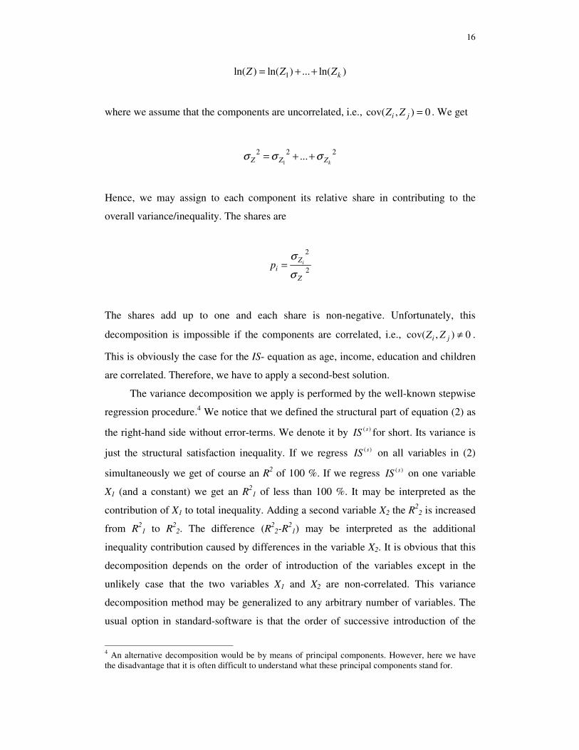
1ln( ) ln( ) ... ln( )kZ Z Z= + +
where we assume that the components are uncorrelated, i.e., cov( , ) 0i jZ Z = . We get
1
2 2 2...kZ Z Zσ σ σ= + +
Hence, we may assign to each component its relative share in contributing to the
overall variance/inequality. The shares are
2
2iZ
iZ
pσ
σ=
The shares add up to one and each share is non-negative. Unfortunately, this
decomposition is impossible if the components are correlated, i.e., cov( , ) 0i jZ Z ≠ .
This is obviously the case for the IS- equation as age, income, education and children
are correlated. Therefore, we have to apply a second-best solution.
The variance decomposition we apply is performed by the well-known stepwise
regression procedure.4 We notice that we defined the structural part of equation (2) as
the right-hand side without error-terms. We denote it by ( )sIS for short. Its variance is
just the structural satisfaction inequality. If we regress ( )sIS on all variables in (2)
simultaneously we get of course an R2 of 100 %. If we regress ( )sIS on one variable
X1 (and a constant) we get an R21 of less than 100 %. It may be interpreted as the
contribution of X1 to total inequality. Adding a second variable X2 the R22 is increased
from R21 to R2
2. The difference (R22-R2
1) may be interpreted as the additional
inequality contribution caused by differences in the variable X2. It is obvious that this
decomposition depends on the order of introduction of the variables except in the
unlikely case that the two variables X1 and X2 are non-correlated. This variance
decomposition method may be generalized to any arbitrary number of variables. The
usual option in standard-software is that the order of successive introduction of the
4 An alternative decomposition would be by means of principal components. However, here we have the disadvantage that it is often difficult to understand what these principal components stand for.
17
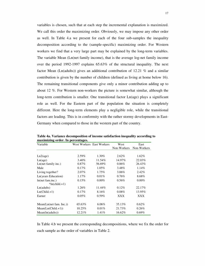
variables is chosen, such that at each step the incremental explanation is maximized.
We call this order the maximizing order. Obviously, we may impose any other order
as well. In Table 4.a we present for each of the four sub-samples the inequality
decomposition according to the (sample-specific) maximizing order. For Western
workers we find that a very large part may be explained by the long-term variables.
The variable Mean (Ln(net family income), that is the average log-net family income
over the period 1992-1997 explains 65.63% of the structural inequality. The next
factor Mean (Ln(adults)) gives an additional contribution of 12.21 % and a similar
contribution is given by the number of children (defined as living at home below 16).
The remaining transitional components give only a minor contribution adding up to
about 12 %. For Western non-workers the picture is somewhat similar, although the
long-term contribution is smaller. One transitional factor Ln(age) plays a significant
role as well. For the Eastern part of the population the situation is completely
different. Here the long-term elements play a negligible role, while the transitional
factors are leading. This is in conformity with the rather stormy developments in East-
Germany when compared to those in the western part of the country.
Table 4a. Variance decomposition of income satisfaction inequality according to maximizing order. In percentages. Variable West Workers East Workers West
Non-Workers East
Non-Workers Ln2(age) 2.59% 1.30% 2.62% 1.62% Ln(age) 3.40% 11.54% 14.97% 22.03% Ln(net family inc.) 0.87% 56.69% 0.86% 26.43% Male 0.17% 1.05% 3.48% 1.14% Living together? 2.07% 1.75% 3.06% 2.42% Ln(years Education) 1.17% 0.01% 0.76% 8.68% ln(net fam.inc.) *ln(child.+1)
0.15% 0.00% 0.56% 0.00%
Ln(adults) 1.26% 11.44% 0.12% 22.17% Ln(Child.+1) 0.17% 8.16% 0.08% 13.95% Earner 0.05% 0.59% XXX XXX Mean(Ln(net fam. Inc.)) 65.63% 6.06% 35.13% 0.62% Mean(Ln(Child.+1)) 10.25% 0.01% 21.73% 0.26% Mean(ln(adults)) 12.21% 1.41% 16.62% 0.69%
In Table 4.b we present the corresponding decompositions, where we fix the order for
each sample as the order of variables in Table 2.

18
Table 4b. Variance decomposition of income satisfaction inequality according to order in Table 2. In percentages. West
Workers East Workers West
Non-Workers East
Non-Workers Ln(age) 0.12% 5.68% 9.18% 2.72% Ln2(age) 1.34% 1.77% 23.41% 50.06% Ln(net family inc.) 56.60% 61.55% 42.99% 29.68% Ln(years Education) 6.48% 1.32% 1.43% 0.68% Ln(adults) 10.32% 14.20% 5.75% 11.98% Ln(Child.+1) 4.77% 4.83% 2.51% 1.94% ln(net fam.inc.) *ln(child.+1)
0.18% 0.02% 0.09% 0.00%
Male 0.28% 1.12% 3.88% 1.00% Living together? 3.41% 2.06% 3.63% 0.38% Earner 0.21% 0.94% 0.00% Mean(Ln(net fam. Inc.)) 13.12% 5.14% 5.05% 0.62% Mean(Ln(Child.+1)) 0.48% 1.37% 0.23% 0.68% Mean(ln(adults)) 2.68% 0.01% 1.85% 0.25%
When we compare Tables 4a. and 4b., we find that the order in which the different
variables are brought into play is very important. Actually, the main burden of the
inequality shifts in Table 4b. to the transitory factors, although the explanation of the
long-term factors being about 16 % is still larger than the 12 % given to the transitory
factors in Table 4a. For non-workers we find that age becomes a very important factor
determining inequality.
Finally, we may take a look at income satisfaction inequality in the whole of
Germany (G). We use the well-known variance decomposition formula, where total
variance is split up into the sum of the two within-group-variances and the between-
groups variance. The two groups are the West-and East-German population in this
case. More precisely we have the identity
( ) ( ) ( ) ( )sat w sat E sat satI G p I W p I E I BetweenEandW= + + (5)
where the p’s stand for the relative population shares. The last term is calculated by
taking the variance of the mean of Western log-income satisfaction and the mean of
Eastern log-income satisfaction with respect to the overall mean log-income
satisfaction. In a similar way we may go on and decompose Isat(W) and Isat(E) with

19
respect to workers and non-workers. That decomposition is tabulated in Table 5. The
results are comparable to those presented in Table 3.
Table 5. Between-group decompositions for Income Satisfaction Inequality (Isat) Population
Shares Group Group Variance of structural
log-income satisfaction
PW = 0.803 West 0.264 PWW = 0.549 West Workers (WW) 0.186 PWNW =0.451 West Non-Workers (WNW) 0.357 Between WW and WNW 0.001 PE =0.197 East 0.265 PEW =0.528 East Workers (EW) 0.141 PENW =0.472 East Non-Workers (ENW) 0.328 Between EW and ENW 0.036 Between E and W 0.010 Germany 0.274
Table 5 shows that the income satisfaction inequality in Germany as a whole is 0.274,
and that there is virtually no difference between the two inequalities in East and West.
The income satisfaction distribution of Non-workers is more unequal than for workers
in both parts of the country.
The same exercise may be done for the objective income inequality. The results
are presented in Table 6. Again, the reader can compare these results with the ones
presented at Table 5. Table 6 illustrates that the objective income inequality in
Germany as a whole is 0.259, which is somewhat smaller than the income satisfaction
inequality. The Westerners suffer from a larger inequality than in the East and the
same holds for the corresponding subgroups of workers and non-workers..
Table 6. Between group decompositions for Income Inequality Population
Shares Group Group Variance of objective
Log-incomes PW = 0.803 West 0.261 PWW = 0.549 West Workers 0.218 PWNW =0.451 West Non-Workers 0.284 Between WW and WNW 0.0132 PE =0.197 East 0.219 PEW =0.528 East Workers 0.173 PENW =0.472 East Non-Workers 0.218 Between EW and ENW 0.0248 Between E and W 0.0063 Germany 0.259

20
Recently Gary Fields (2002) suggested another decomposition, which may be
succinctly described as follows. If there holds 1 1 ... k kZ Z Zβ β ε= + + + , there also
holds
1 1var( ) cov( , ) ... cov( , ) var( , )k kZ Z Z Z Z Zβ β ε= + + +
Division by var( )Z yields
1 ... 1kp p pε+ + + =
This is another way to define inequality or variance shares. The advantage of this
decomposition is that the shares do not depend on the order of introduction of the
variables. They are uniquely defined, thereby avoiding the element of arbitrariness,
which is inherent to the stepwise procedure, followed above. However, the price to be
paid is that the shares p may be negative or larger than one, which makes
interpretation cumbersome. It is therefore, that we did not use the Fields-
decomposition.
5. Conclusions
In this paper we extended the objective income concept by defining the subjective
income satisfaction concept. Similarly we extend the objective income inequality
concept by defining an income satisfaction inequality concept. The Isat measure differs
from objective measures of inequality as individual subjective satisfaction with
income is used instead of objective income. In other words, the paper presents
estimates for feelings of income inequality. The measure Isat includes objective income
inequality as a special case, namely, when subjective income satisfaction and income
are identical.
We find that only a relatively small part of Isat can be attributed to observed
factors. This does not necessarily imply that there would be no other observable
causes of inequality. It may be that the specification presented in Table 2 omitted
relevant observable variables. Nevertheless, this is not very likely, given the large
range of variables available in the GSOEP and the extensive research we did trying

21
different possible specifications. Even if the variance due to observable factors is
rather small, it is interesting to look at it, given that the objective variables are the
only ones, which policy makers can take into account. The role of income in
explaining income satisfaction inequality is not insignificant but it is not the only
causing factor. The number of people in the household and the age distribution are
important as well. Thus, even if objective income inequality remains certainly an
important statistic to monitor the societal distribution process, this exercise shows that
psychological feelings of inequality are relevant as well. Evidently, this research
should be repeated for other populations, before we may generalize the findings of
this paper.
This paper contributes to the literature of inequality by presenting an income
satisfaction concept, which can be compared to objective measures of inequality.
Income satisfaction inequality differs from the established measures of inequality by
using individual perceptions as a basis to make incomes comparable. The traditional
measures of inequality introduce subjectivism via intuition by, for example, imposing
family equivalence scales (such as the Oxford/OECD scale) or by introspection in
choosing a concrete welfare function specification with a numerically determined
risk/inequality aversion parameter (Atkinson, 1970). The introduction of income
satisfaction does not imply that objective measurement should be replaced by
subjective concepts throughout, but only that both measures have a different role to
play. The subjective concept is in our opinion a valuable addition to the family of
inequality measures.

22
References
Aitchison, J. and J.A.C. Brown, 1960. The Lognormal Distribution. Cambridge
University Press, London.
Argyle, M., 1999. Causes and correlates of happiness. In: D. Kahneman, E. Diener
and N. Schwarz (eds.). Well-Being: The Foundations of Hedonic Psychology.
Russell Sage Foundation, New York. Chapter 18.
Atkinson, A.B., 1970. On the measurement of inequality. Journal of Economic
Theory, 2: 244-263.
Atkinson, A.B. and F. Bourguignon (eds), 1999. Handbook of Income Distribution,
North Holland, Amsterdam.
Baker, M., 1997. Growth-rate heterogeneity and the covariance structure of life-cycle
earnings. Journal of Labor Economics, 15:338-375.
Brickman, P. and D.T. Campbell, 1971. Hedonic relativism and planning the good
society. In: M.H. Apley (ed.). Adaptation-level theory: A symposium. Academic
Press, New York. Pages: 287-302.
Cantril, H., 1965. The pattern of human concerns. Rutgers University Press. New
Brunswick.
Clark, A. E. and A.J. Oswald, 1994. Unhappiness and unemployment. Economic
Journal, 104: 648-659.
Clark, A. E. and A.J. Oswald,1996. Satisfaction and comparison income. Journal of
Public Economics, 61: 359-381.
Cowell, F.A., 1999. Measurement of Inequality in Atkinson, A.B. and F. Bourguignon
(eds), 1999. Handbook of Income Distribution, North Holland, Amsterdam.
Dalton, H., 1920. The Measurement of the Inequality of Incomes. Economic Journal,
30: 348-361.
Dickens, R. (2000). The evolution of individual male wages in great-Britain:1975-
1995. The Economic Journal,110: 27-49.
Diener, E. and R.E. Lucas, 1999. Personality and subjective well-being. In: D.
Kahneman, E. Diener and N. Schwarz (eds.). Well-Being: The Foundations of
Hedonic Psychology. Russell Sage Foundation, New York. Chapter 11.
Diener, E., E.M Suh, R.E. Lucas and H.L. Smith, 1999. Subjective well-being: Three
decades of progress. Psychological Bulletin, 125: 276-302.

23
Di Tella, R., R.J. MacCulloch and A.J. Oswald, 2001. Preferences over Inflation and
Unemployment: Evidence from Surveys of Happiness. American Economic
Review, 91: 335-341.
Easterlin, R.A., 2000. The worldwide standard of living since 1800. The Journal of
Economic Perspectives, 14: 7-26.
Ferrer-i-Carbonell, A. and B.M.S. Van Praag, 2001. The subjective costs of health
losses due to chronic diseases. An alternative model for monetary appraisal. Health
Economics, 11: 709-722.
Ferrer-i-Carbonell, A., 2002. Income and Well-being: An Empirical Analysis of the
Comparison Income Effect, Tinbergen Institute Working Paper 2002-019.
Fields, G.S., 2002. Accounting for Income Inequality and Its Change: A New Method,
with Application to the Distribution of Earnings in the United States, forthcoming
in Research in Labor economics.
Friedman, M., 1957. A theory of the consumption function. Princeton University
Press, Princeton, NJ.
Frey, B.S. and A. Stutzer, 2000. Happiness, economy and institutions. Economic
Journal, 110: 918-938.
Frijters, P., 2000. Do individuals try to maximize general satisfaction? Journal of
Economic Psychology, 21: 281-304.
Gini, C., 1912. Variabilita e Mutabilita, Bologna, Italy.
Helson, H., 1964. Adaptation level as frame of reference for prediction of
psychological data. The American Journal of Psychology, 60: 1-29.
Hunt, J., 1999. Determinants of non-employment and unemployment durations in East
Germany. NBER Working Paper Series No. 7128, Cambridge MA.
Hunt, J., 2000. Why do people still live in East? The Institute for the Study of Labor
(IZA) Discussion Paper No. 123, Bonn, Germany.
Kahneman, D., E. Diener and N. Schwarz (eds.), 1999. Foundations of Hedonic
Psychology: Scientific Perspectives on Enjoyment and Suffering. Russel Sage
Foundation, NY.
Kapteyn, A. and F.G. Van Herwaarden, 1980. Independent welfare functions and
optimal income distribution. Journal of Public Economics, 14: 375-397.
Likert, R., 1932. A technique for the measurement of attitudes. Archives of
Psychology, 140:55.

24
Lillard, L. and R. Willis, 1978.. Dynamic aspects of earnings mobility. Econometrica,
46: 985-1012.
Mundlak, Y., 1978. On the Pooling of Time Series and Cross Section Data.
Econometrica, 46: 69-85.
Ng, Y-K., 1997. A Case for Happiness, cardinalism, and interpersonal comparability.
The Economic Journal, 107: 1848-1858.
Pannenberg, M., 1997. Documentation of Sample Sizes and Panel Attrition in the
German Socio Economic Panel (GSOEP). Discussion Paper No. 150, Deutsches
Institut für Wirtschaftsforschung, Berlin.
Plug, E., B. van Praag, P. Krause, and G, Wagner, 1997. Measurement of poverty:
Exemplified by the German case. In: N. Ott and G.G. Wagner (ed), Income
inequality and poverty in Eastern and Western Europe. Physica-Verlag,
Heidelberg. Pp. 69-89.
Rao, C.R., 1973. Linear Statistical Inference and its Applications, Wiley & Sons,
New York.
Sen, A.K., 1973. On economic inequality. Reprinted 1997. Clarendon Press, Oxford.
Sen, A.K., 1999. The possibility of social choice. American Economic Review, 89:
349-378.
Silber, J. (ed.). 1999. Handbook of income inequality measurement. Kluwer
Academic: Dordrecht, the Netherlands.
Theil, H., 1967. Economics and Information Theory, North-Holland Publishing Cy.,
Amsterdam.
Theil, H., 1979. The measurement of inequality by components of income. Economics
Letters, 2: 197-199.
Van Praag, B.M.S., 1971. The welfare function of income in Belgium: an empirical
investigation. European Economic Review, 2: 337-369.
Van Praag, B.M.S., 1978.The Perception of Income Inequality. In: W. Krelle and A.F.
Shorrocks (eds.). Personal Income Distribution. North-Holland Publishing
Company, Amsterdam. Pages: 113-136.
Van Praag, B.M.S., 1991. Ordinal and cardinal utility: an integration of the two
dimensions of the welfare concept. Journal of Econometrics, 50: 69-89.
Van Praag, B.M.S., P. Frijters, and A. Ferrer-i-Carbonell, 2003. The anatomy of well-
being. Journal of Economic Behavior and Organization, 51: 29-49.

25
Wagner, G.G., Burkhauser, R.V., Behringer, F., 1993. The English language public
use file of the German Socio-Economic Panel. Journal of Human Resources, 28:
429-433.

IZA Discussion Papers No.
Author(s) Title
Area Date
840 E. Koskela R. Stenbacka
Equilibrium Unemployment Under Negotiated Profit Sharing
1 08/03
841 B. H. Baltagi D. P. Rich
Skill-Biased Technical Change in U.S. Manufacturing: A General Index Approach
1 08/03
842 M. Svarer M. Rosholm J. R. Munch
Rent Control and Unemployment Duration 3 08/03
843 J. J. Heckman R. Matzkin L. Nesheim
Simulation and Estimation of Hedonic Models 6 08/03
844 D. Sliwka
On the Hidden Costs of Incentive Schemes 1 08/03
845 G. Dewit H. Görg C. Montagna
Should I Stay or Should I Go? A Note on Employment Protection, Domestic Anchorage, and FDI
2 08/03
846 D. de la Croix F. Docquier
Diverging Patterns of Education Premium and School Attendance in France and the US: A Walrasian View
6 08/03
847 B. R. Chiswick Jacob Mincer, Experience and the Distribution of Earnings
1 08/03
848 A. Chevalier G. Conlon
Does It Pay to Attend a Prestigious University? 6 08/03
849 W. Schnedler Traits, Imitation, and Evolutionary Dynamics 5 08/03
850 S. P. Jenkins L. Osberg
Nobody to Play with? The Implications of Leisure Coordination
5 08/03
851 J. D. Angrist Treatment Effect Heterogeneity in Theory and Practice
6 08/03
852 A. Kugler M. Kugler
The Labor Market Effects of Payroll Taxes in a Middle-Income Country: Evidence from Colombia
1 08/03
853 I. Ekeland J. J. Heckman L. Nesheim
Identification and Estimation of Hedonic Models 6 08/03
854 A. Ferrer-i-Carbonell B. M. S. Van Praag
Income Satisfaction Inequality and its Causes 3 08/03
An updated list of IZA Discussion Papers is available on the center‘s homepage www.iza.org.