Income Inequality: TheoryPa

ul’s

Mar

gina

l Util

ity

Pete

r’ s M

argi

nal U

tility

O O’I*

Income Inequality in the US Over Time

Question: What fraction of all household income is received by the poorest fifth (quintile

1)? The second-poorest? etc. Q5/Q1 is the ratio of the income received by the richest

fifth to income received by the poorest fifth.

Fraction of Pretax Income Received By Quintile Q5/Q1

Year 1 2 3 4 5

1968 4.2 11.1 17.5 24.4 42.8 10.21975 4.4 10.5 17.1 24.8 43.2 9.81980 4.3 10.3 16.9 24.9 43.7 10.21985 4.0 9.7 16.3 24.6 45.3 11.31990 3.9 9.6 15.9 24.0 46.6 11.9

1993 3.6 9.0 15.1 23.5 48.9 13.61996 3.7 9.0 15.1 23.3 49.0 13.21999 3.6 8.9 14.9 23.2 49.4 13.7

Source: US Census Bureau, Report P60-209, Table C.

Facts:

- “Hollowing” of distribution: income received by Q3 has substantially declined- Income of Q1 declined 1968-1993, has stayed about the same since 1993- Income received by Q5 increased sharply 1968-1993, has stayed same since

93- Tax policy:

- Roughly constant 1968-1980- Sharp cuts at the top in 1980s- Substantial tax increases at the very top (top 1 percent) in the 1990s- Substantial tax cuts at the bottom (Earned Income Tax Credit) in 1990s

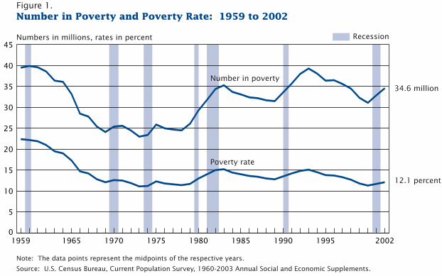
U.S. Census Bureau Poverty in the United States: 2002 3

Figure 1.Number in Poverty and Poverty Rate: 1959 to 2002

Note: The data points represent the midpoints of the respective years.

Source: U.S. Census Bureau, Current Population Survey, 1960-2003 Annual Social and Economic Supplements.

Numbers in millions, rates in percent

0

5

10

15

20

25

30

35

40

45

2002 19951990198519801975197019651959

Recession

34.6 million

12.1 percent

Number in poverty

Poverty rate

The estimates in this report are based on theCurrent Population Survey (CPS) 2001, 2002, and2003 Annual Social and Economic Supplement(ASEC) and provide information for calendar years2000, 2001, and 2002, respectively.

For the first time in 2003, CPS respondents were askedto identify themselves in one or more racial groups;5

previously they had to choose one. This change com-plicates year-to-year comparisons. We do not knowhow people who reported more than one race in 2002previously reported their race. Therefore, there is nosingle way to compare changes to poverty by race.

Table 1 compares last year’s single-race figures withtwo different figures this year: one comparison isbased on those who reported one race alone and theother is based on those who reported either that raceonly or that race and at least one other race. Forexample, this year’s poverty report will compare the2001 poverty figures for Blacks with 2002 povertyfigures for those who reported themselves as:

1. Black alone, did not report any other race, and

2. Black alone or in combination with some otherrace(s).

The Census Bureau will provide year-to-year com-parisons for each racial group, with the exception ofAmerican Indians and Alaska Natives, and NativeHawaiians and Other Pacific Islanders, who will notbe examined separately (because the sample wasnot sufficiently large).

New Racial Groups

5 OMB establishes the official guidelines for the collection andclassification of data for race (including the option for respondentsto mark more than race) and Hispanic origin. Race and Hispanic ori-gin are treated as separate and distinct concepts in accordance withOMB’s guidelines. For further information, see www.whitehouse.gov/omb/ombdir15.html.

Source:

“Income Distribution and Poverty in Selected OECD Countries,” OECD Economics Department Working Paper No. 189, p. 39

http://www.oecd.org/eco/eco

Urban–Brookings Tax Policy CenterISSUES AND OPTIONS

6

sunsets. The provision relieving sometaxpayers from paying the compli-cated AMT, for example, expires after2004. Absent a change in law, 35 mil-lion taxpayers will be subject to theAMT by 2010 (JCT 2001), and familieswith children will be more than twiceas likely as childless households tofall prey to this tax. Such a bleak out-come may seem politically infeasible,but an AMT fix is also problematicbecause it would cost hundreds ofbillions of dollars (Burman, Gale, andRohaly 2002).

In addition to the AMT, policy-makers should seriously reassess theunnecessary complexity facing lower-income families when they preparetheir taxes. EGTRRA did simplify theEITC. But it missed an opportunity tosimplify the complicated refundablechild tax credit; indeed, it made com-puting the credit more complex.

Other areas worth simplifying arethe various child-related tax benefits.Better integrating the definitions,requirements, and administration ofthese benefits would make many tax-payers’ lives easier. For example,combining personal exemptions forchildren with the child tax credit andthe EITC into a single child-assistance

tax credit would simplify many fami-lies’ tax preparation (Ellwood andLiebman 2000). This change wouldalso make the tax system more pro-gressive, since low-income familiesgain more from refundable tax creditsthan from deductions and nonrefund-able credits. Replacing personalexemptions for adults with higherstandard deductions would also sim-plify and add progressivity to the sys-tem (Feenberg and Skinner 1993).Since most high-income householdstend to itemize, larger standarddeductions would mostly benefitlower- and middle-income families.

Endnotes

1. This brief is a very abbreviated version ofBurman, Maag, and Rohaly (2002). For amore comprehensive discussion ofEGTRRA, see Gale and Potter (2002).

2. The cost includes both tax revenuedecreases and increased outlays on refund-able tax credits (JCT 2001).

3. At its maximum, the child tax credit isworth $772 (in 2000 dollars).

4. Previously, the child tax credit was onlyrefundable to families with three or morechildren to the extent that the employershare of Social Security taxes plus individ-ual income taxes exceeded a family’s EITC.

This complicated provision remains ineffect after EGTRRA, even though it willbenefit few people and will continue toconfuse many.

5. The taxpayer’s earnings exceed $10,000 by$6,000; 10 percent of $6,000 equals $600.See Greenstein (2001) for an excellent dis-cussion of the issues surrounding theexpansion of the child tax credit and theEITC.

6. For more on the logic behind the refund-able child tax credit and its effect on poorfamilies and work incentives, see Sawhilland Thomas (2001a; 2001b).

7. The CDCTC may also be used to pay forthe costs of care for a disabled or elderlydependent.

8. After adjusting for inflation, the maximumallowable expense per child declines from$2,400 in 2000 to $2,316 in 2010.

9. For example, the phaseout rate for taxpay-ers with two or more qualifying children is21.06 percent. That is, for every $100earned, taxpayers lose $21.06 of EITC,amounting to a surtax of 21.06 percent inthe phaseout range.

10. Wheaton (1998) discusses EITC marriagepenalties and some options to mitigatethem.

11. The couple would also owe more tax beforecredits by virtue of being married, so thatits total marriage penalty would exceed$3,186.

12. The lower tax rates for upper-income tax-payers also roughly double the number ofpeople subject to the AMT over the next

TABLE 5. Estimated Distribution of Income and Estate Tax Changes, 2010 Calendar Year

Income Tax Estate Taxa

Percent of PercentPercent of Total Tax Percentage Total Tax Percentage Total Income Change in

AGI Class Total Change of Change of and Estate After-Tax(2001$) Returns (Millions) Total (Millions) Total Tax Cut Income

Less than $10,000 19.4 –988 0.6 0 0.0 0.4 0.52$10,000–$20,000 17.4 –10,717 6.3 0 0.0 4.8 2.22$20,000–$30,000 13.1 –13,852 8.2 0 0.0 6.2 2.47$30,000–$40,000 9.8 –11,853 7.0 0 0.0 5.3 2.07$40,000–$50,000 7.5 –11,060 6.5 –200 0.4 5.1 2.03$50,000–$75,000 12.3 –22,798 13.5 –300 0.6 10.4 1.86$75,000–$100,000 7.7 –18,772 11.1 –1,200 2.2 9.0 1.89$100,000–$200,000 9.4 –16,628 9.8 –11,400 21.3 12.6 1.47$200,000 and over 2.7 –62,132 36.8 –40,300 75.5 46.1 5.59

Total 100.0 –168,924 100.0 –53,400 100.0 100.0 2.69

Sources: Urban-Brookings Tax Policy Center Microsimulation Model and authors’ calculations. Note: For model description, see notes on Table 6.a. Assumes that estate taxes are distributed as reported by the Treasury Department, Office of Tax Analysis in table 12 of Cronin (1999). Treasury reports the distribution interms of family economic income (FEI), a broader measure than AGI. The FEI quintile distribution as reported by Treasury was converted to AGI quintiles and then assignedto the dollar income classes shown in the table. See Burman (2001) for more details.

“I’ve been thinking about the flat tax and how it wouldbe a hardship for the poor, and I can live with that.”