Income Distribution and Housing Prices:

An Assignment Model Approach

Niku Määttänen

ETLA and HECER∗Marko Terviö

Aalto University and HECER†

December 9, 2013‡

Abstract

We present a framework for studying the relation between the distributions of

income and house prices that is based on an assignment model where households are

heterogeneous by incomes and houses by quality. Each household owns one house

and wishes to live in one house; thus everyone is potentially both a buyer and a

seller. In equilibrium, the distribution of prices depends on both distributions in

a tractable but nontrivial manner. We show how the impact of increased income

inequality on house prices depends on the shapes of the distributions, and can be

inferred from data. In our empirical application we find that increased income

inequality between 1998 and 2007 had a negative impact on average house prices in

6 US metropolitan areas. JEL: D31, R21.

∗niku.maattanen@etla.fi,The Research Institute of the Finnish Economy (ETLA) and Helsinki Center

for Economic Research.†marko.tervio@aalto.fi, Aalto University School of Economics and Helsinki Center for Economic Re-

search.‡We thank Essi Eerola, Pauli Murto, Ofer Setty, Otto Toivanen, Juuso Välimäki, and seminar partic-

ipants at Bonn, ECARES, EIEF, EUI, Mannheim, Munich, NHH Bergen, NorMac, Nottingham, Stock-

holm, SOFI, UAB, and Zurich for useful suggestions. Määttänen thanks Suomen arvopaperimarkkinoiden

edistämissäätiö and the Academy of Finland and Terviö thanks the European Research Council for fi-

nancial support.

1

1 Introduction

A central feature of the housing market is that housing is not a fungible commodity but

comes embedded in indivisible and heterogeneous units. What people refer to as “houses,”

are really bundles of land and structures. The quality of land is inherently heterogeneous

because locations differ in their attractiveness due to fixed factors such as distance from

the center and view of the sea. The supply of structures is more or less fixed in the short

term, and only partly adjustable in the medium term. Quality of structures can also have

a fixed component, due to zoning restrictions or the scarcity value of vintage architecture.

At the same time, housing is a normal good, as the more wealthy spend more on housing.

Given the indivisibility and heterogeneity of houses, it is natural to consider the hous-

ing market as an assignment problem. Yet, assignment models are not a standard tool

in applied work on housing economics. One reason may be that in the standard assign-

ment model agents are ex ante divided into two distinct classes, such as "buyers" and

"sellers". The two-sidedness assumption is natural in many markets, for example when

firms are matched with workers, but is problematic in the housing market where most

households are potentially both sellers and buyers. Furthermore, standard assignment

models assume transferable utility and so preclude income effects. In the housing market,

however, income effects may be significant since housing takes up a large part of household

expenditure.

In this paper, we present a one-sided assignment model with non-transferable utility,

where houses are heterogeneous by quality and households are heterogeneous by income.

Each household owns one house and wishes to live in one house; thus households’ reserva-

tion prices as sellers depend on the opportunities available to them as buyers. We model

a single metropolitan region, where the set of households is fixed. The distributions of in-

come and house quality are exogenous, while the distribution of house prices and therefore

wealth is endogenous, with the exception of the cheapest or “marginal” house. In general,

the initial joint distribution of houses and income is arbitrary, which results potentially

in a lot of trading between households. Equilibrium prices depend on the properties of

the joint distribution, not just on the marginal distributions of income and house quality.

We show the existence of equilibrium prices under an arbitrary initial endowment. For

most of the paper we focus on the equilibrium prices that emerge after all trading oppor-

tunities have been exploited. Equilibrium prices can then be solved explicitly from the

joint distribution of wealth and house quality and the parameters of the utility function.

We use the equilibrium conditions to derive analytical results for the impact of income

distribution on the distribution of house prices.

2

According to our theoretical results the impact of increased income inequality on top

(as well as average) house prices is ambiguous. The intuition for why increase in in-

come inequality leads to lower prices at the bottom of the quality distribution is clear:

if low-income households have less income they bid less for low-quality houses. However,

in equilibrium, any changes in prices spill upwards in the quality distribution. This is

because the binding outside opportunity of any (inframarginal) household is that they

must want to buy their equilibrium match rather than the next best house. The equilib-

rium price gradient–the price difference between two "neighboring" houses in the quality

distribution–is pinned down by how much the households at the relevant part of the in-

come distribution are willing to pay for the quality difference. The price of any particular

house is then given by the summation of all price gradients below, plus the price of the

marginal house. Thus, while an increase in incomes at the top increases the local price

gradient, the lower prices at the bottom put downward pressure on prices above. It is

therefore possible for all house prices to go down in response to an increase in inequality.

In order to illustrate the mechanisms of the model and to evaluate their quantitative

importance we apply our model to data from the American Housing Survey (AHS) in

1998 and 2007. We assume that all households prefer to live in their current house under

current market prices. Under this “post-trade” interpretation of data the distribution

of unobserved house qualities can be inferred as the distribution that gives rise to the

observed price distribution as the equilibrium outcome of our model. The inferred distri-

bution of house qualities can be used to generate counterfactuals. This setup is at its most

useful in analyzing changes or policies that may be at least partly capitalized into house

prices, such as income transfers and housing cost subsidies; we discuss other potential

applications of our model in the end.

We find that a suitably parametrized constant elasticity of substitution (CES) utility

function allows us to roughly match the observed change in the price distribution under

the assumption that it was caused by the observed change in incomes while unobserved

house qualities remained unchanged. We first use the calibrated model to illustrate how

the income elasticity of housing demand depends on the quality and income distributions,

and varies between households, despite homogeneous CES preferences. Intuitively, how

much more one would spend on housing following an increase in income depends on the

additional housing quality that one extra dollar can buy; this in turn varies over the

distribution, as it depends both on available qualities and on the incomes of competing

buyers and sellers.

We then consider counterfactual income distributions for 2007 where all incomes grow

uniformly since 1998 at the same rate as the actual mean income in the same metropolitan

3

region. We compare house prices that result from the counterfactual income distributions

with the prices resulting from the actual income distributions, while holding constant

the population and the housing supply in each city. This exercise can be seen as a way

to disentangle the short or medium run impact of increased income inequality on house

prices from changes in other house price determinants.

Depending on the region, counterfactual income distributions result in house prices

that are on average 0 − 10% higher than house prices resulting from actual income dis-

tributions. (This excludes any changes in the top 3% of the price distribution, which is

excluded due to top coding). This implies that the increase in inequality has resulted in

lower prices on average than would have prevailed under uniform income growth, but the

impact is modest in magnitude compared to the overall change in prices. The contribution

of uneven income growth on house prices has been positive only within the top decile,

with magnitudes of up to 12%. We also compare our results to those that one would

obtain using a two-sided model or a much simpler model without indivisibilities.

In the next section we discuss related literature. In Section 3 we present the model

and our theoretical results. In Section 4 we show how the model can be used for inference

and counterfactuals. The empirical application is presented in Section 5, and Section 6

concludes.

2 Related Literature

Assignment models are models of perfectly competitive matching markets that focus on

the combined impact of indivisibilities and two-sided heterogeneity; for a review see Sat-

tinger (1993). All other frictions, such as imperfect information or transaction costs, are

assumed away. Both sides of the market are assumed to have a continuum of types, so

there is no market power or bargaining as all agents have arbitrarily close competitors.

Assignment models typically include an assumption of a complementarity in production,

which results in assortative matching. Resulting equilibrium prices depend on the shapes

of the type distributions on both sides of the market but in a reasonably tractable way.

Assignment models have usually been applied to labor markets, where the productive com-

plementarity is between job types and worker types, as in Sattinger (1979) and Teulings

(1995).

There exists a large literature on two-sided assignment, where agents are ex ante

divided into two distinct classes, such as "buyers" and "sellers," are matched.1 A two-

1For recent theoretical literature see, for example, Legros and Newman (2007) and Caplin and Leahy

(2010).

4

sided variant of our model can be obtained by assuming that houses are owned by a

separate class of agents who do not themselves consume houses; it is essentially the setup

analyzed by to Braid (1981), to which we return in section 3.4. Our model differs from

previous assignment models by featuring both one-sided matching and non-transferable

utility. There is no complementarity in the usual sense, but equilibrium nevertheless

involves assortative matching by wealth and house quality, essentially because housing

is a normal good. We don’t restrict the shapes of the distributions (beyond minimal

regularity conditions). In the empirical application we can then use a nonparametric

method to infer the unobserved type distribution and to construct counterfactuals similar

to Terviö (2008).

Assignment models are rarely used in applied work on housing economics. An inter-

esting exception is Landvoigt, Piazzesi, and Schneider (2012). They use a two-sided as-

signment model with concave utility to motivate a nonlinear relationship between housing

quality and house prices, which they incorporate into an intertemporal model of housing

demand. They employ a calibrated version of their model to study the housing market

of San Diego county, California, during the 2000s boom. Using the model, they infer the

role of cheap credit from the cross section of capital gains by house quality. Their main

result is that cheaper credit for poor households increased house prices substantially at

the low end of the market. Their model is in the traditional two-sided assignment model

framework, where the two sides of the market–buyers and houses–are separate popu-

lations, and the prices of other houses do not affect the sellers. In our one-sided model

buyers are also sellers, and households’ reservation prices as sellers are intricately related

to the prices (and qualities available) they face as buyers.

In the theoretical matching literature housing has been used as the motivating example

of an indivisible good that needs to be “matched” one-to-one with the buyers. The classic

reference is Shapley and Scarf (1974), who present a model where houses are bartered by

a discrete set of households who are each endowed with and each wish to consume exactly

one house. They show that, regardless of the preference orderings by the households,

there always exists at least one equilibrium allocation. Quinzii (1984) and Gale (1984)

proved the existence of an equilibrium allocation when, in addition to the indivisible good,

there is also a second continuous good or “money.”2 We get more results by imposing more

structure, most importantly we assume homogeneous preferences with housing as a normal

good. Also, we assume that there is a continuum of households, which together with the

common preference ordering allows us to use calculus for analysis and for an intuitive

2Quinzii (1984) proved under slightly less general assumptions that equilibrium allocations also coin-

cide with the core.

5

understanding of comparative statics. With this structure the model can be mapped in a

manageable way to the observed joint distribution of house prices and household incomes.

There is a long tradition in explaining heterogeneous land prices in urban economics,

going back to the classic Von Thünen model, and Alonso (1964). In these models the

exogenous heterogeneity of land is due to distance from the urban center. The focus

is on explaining how land use is determined in equilibrium, including phenomena such

as parcel size and population density. In modern urban economics3 there are also some

models with income effects. Usually heterogeneity of land is modeled as a transport cost,

which is a function of distance from the center, and price differences between locations

are practically pinned down by the transport cost function.

Recent models with location choice and endogenous land prices include one by Epple

and Sieg (1999), who estimate a structural model where public good provision is endoge-

nous akin to Tiebout (1956). Glazer, Kanniainen, and Poutvaara (2008) analyze the

effects of income redistribution in a setup where heterogeneous land is owned by absentee

landlords. They show that the presence of (uniformly distributed) heterogeneity miti-

gates the impact of tax competition between jurisdictions because taxation that drives

some of the rich to emigrate also leads them to vacate high-quality land, allowing the

poor to consume better land than before. Eeckhout, Pinheiro, and Schmidheiny (2013)

consider the sorting of worker types across cities, while allowing for within-city sorting in

a monocentric city model. In Ortalo-Magné and Prat (2010) household location choice

between regions is modeled as part of a larger portfolio problem, where each region has

a fixed amount of (infinitely divisible) housing capital. Different regions offer different

income processes, so location decisions as well as house prices are affected by hedging

considerations.

Most dynamic macroeconomic models with housing assume that housing is a homoge-

nous malleable good. In any given period, there is then just one unit price for housing.

An exception is the property ladder structure used by Ortalo-Magné and Rady (2006)

and Ríos-Rull and Sanchez-Marcos (2008), where there are two types of houses: relatively

small “flats” and bigger “houses”. For our purposes, a two-type distribution would be far

too coarse. Most macro housing literature focuses on the time series aspects of a general

level of housing prices, and abstracts away from the cross-sectional complications of the

market.

There is also a literature that is concerned with the dispersion of house prices between

cities, while abstracting away from heterogeneity within cities. Van Nieuwerburgh and

Weill (2010) study house price dispersion across US cities using a dynamic model, where

3See, for example, the textbook by Fujita (1989).

6

there is matching by individual ability and regional productivity. Within each city housing

is produced with a linear technology, but there is a city-specific resource constraint for

the construction of new houses. This causes housing to become relatively more expensive

in regions that experience increases in relative productivity. Gyourko, Mayer, and Sinai

(2006) have a related model with two locations and heterogeneous preferences for living in

one of two possible cities. One of the cities is assumed to be a more attractive “superstar”

city in the sense that it has a binding supply constraint for land. An increase in top

incomes results in more competition for scarce land, thus leading the price of houses in

the superstar city to go up. Moretti (2013) presents a model where changes in relative

housing prices between two cities can be affected by productivity (demand for labor)

and location preference. He finds that a fifth of the observed increase in college wage

premium between 1980 and 2000 was absorbed by higher cost of housing, and that the

most plausible cause for this is an increase in demand for high-skill workers in regions

that attracted more high-skill workers. By contrast, Diamond (2012) finds that well-

being inequality grew more than wage inequality over the same period, once accounting

for endogenous change in local amenity levels.

3 Model

We model a one-period pure exchange economy, where a unit mass of households consume

two goods, housing and a composite good. Preferences are described by a utility function

, same for all households. Houses come in indivisible units of exogenous quality, and

utility depends on the quality of the house, denoted by . Every household is endowed

with and wishes to consume exactly one house. A household’s endowment of the composite

good can be interpreted as its income. There are no informational imperfections, or

other frictions besides the indivisibility of houses. We assume standard preferences: is

strictly increasing, differentiable, and strictly quasi-concave.

The aim is to find equilibrium prices for a continuum of house types, given the en-

dowment and the preferences. The aggregate endowment can be described by the joint

distribution of households, , over the consumption space, S = [0 1]×R+. We assumethat households are distributed without gaps or atoms over [0 1]× [0 1]. Figure 1 de-picts the consumption space of this economy, with horizontal dimension representing the

quantile in the marginal distribution of house quality = (), and vertical dimension

representing the composite good or "consumption" for short.

Consider first the problem of an individual household. Figure 1 shows the budget

curve of a household endowed with a bundle {e e}, its shape determined by the price7

Figure 1: Consumption space. Horizontal axes depicts the quantile of house quality ()

and vertical axes the level of non-housing consumption . The shaded area is the budget set

of a household with endowment {e } and optimal choice {∗ ∗}. A set of indifferencecurves is depicted (for ( ) = ); their apparent non-convexity is due to showing the

quantile of on horizontal axes.

function which households take as given. For this household, the very best houses are

outside its budget set, because negative consumption is not feasible. The optimal bundle

{∗ ∗} is where the household gets to the highest indifference curve in its budget set.This household is relatively well endowed in the composite good and would therefore give

up some of it in order to trade up to a better house. Formally, the household selects a

house of type ∗ = argmax ( e+ (e)− ()), thus leaving ∗ = e+ (e)− (∗) for

consumption.

In equilibrium, the price function must be such that i) all households choose their

utility-maximizing while taking as given and ii) the resulting allocation is feasible.

The indivisibility of houses means that the distribution of house types (the marginal

distribution ) cannot be altered by trading. Thus feasibility requires that, for all , the

8

marginal density of households choosing to live in house type is equal to the marginal

density of households endowed with type .

Equilibrium conditions To state the equilibrium conditions more formally, first define

the no-trade level of income for a household endowed with a house of type and facing

price function

∗ () =

½ st. = arg max

∈[01] ( + ()− ())

¾. (1)

We later show that, for equilibrium , ∗ is single-valued almost everywhere. Now denote

the budget set of a household endowed with {e e} by (e e) = {( ) ∈ S st. () + ≤ (e) + e} . (2)

Finally, the demand and supply of every type of house is equal and all households are

maximizing utility under prices whenZ Z(∗max ∗(∗))

( )dd = (∗) (3)

for all ∗ ∈ [0 1]. (We use to denote the density associated with .) Then, by Walras’Law, the total consumption of also equals its total endowment.

In terms of Figure 1, the resource constraint requires that the proportion of households

with an endowment located below the budget curve for the endowment {∗ ∗} is equal to (

∗), the proportion of houses that are of quality ∗ or less. The resource constraints

involve double integrals, but, by discretizing the house types, the equilibrium can be

solved numerically using standard methods. For most of this paper we will focus on the

post-trade allocation, which simplifies the analysis considerably, and allows us to derive

closed-form results for the comparative statics of the price distribution. To get there we

need two lemmas.

Lemma 1 In equilibrium there is positive assortative matching (PAM) by household

wealth and house quality.

That is, in equilibrium, the ranking of households by wealth and by house quality

must be the same. The proof is in the Appendix. In short, the diminishing marginal

rate of substitution guarantees PAM: of any two households, the wealthier must live in

the better house, or else the two could engage in mutually profitable trade. The twist

here is that the ordering by wealth is not known beforehand, because the value of the

9

house is endogenous. So, despite PAM, the equilibrium allocation is not obvious and

depends on the shape of the joint distribution of . The benefit of Lemma 1 is that it

guarantees that the equilibrium allocation is essentially one-dimensional, so we can index

both households and houses by the house quality quantile . We prove the existence of

an equilibrium allocation in the Appendix under a finite (but arbitrarily large) number of

house types. The equilibrium is associated with unique prices, up to an additive constant

that can be interpreted as the opportunity cost of the worst house.

Lemma 2 In equilibrium all households ∈ [0 1] are located on a curve {() ∗()} inthe consumption space that is continuous almost everywhere. If there are jumps they are

upwards.

This follows directly from Lemma 1: as wealth and therefore utility are increasing in ,

downward jumps in ∗ (as a function of ) are ruled out. Similarly, allocations supported

over any thick region in consumption space would violate PAM. Only upward jumps in

∗ are not ruled out, but there can only be a countable number of them or else ∗ would

not stay finite. Hence ∗ is continuous almost everywhere.4 However, ∗ does not have to

be increasing.5

The increasing curve in Figure 2 depicts the equilibrium allocation for a lognormally

distributed endowment with positive correlation. Households below the curve are the net

suppliers of quality: they are endowed with a relatively high quality house and trade down

in order to increase their consumption of the composite good. Households endowed with

a house of quality () and income level () = ∗() do not trade. The end points of the

equilibrium curve are necessarily {0 0} and {1 1}, as the unambiguously poorest andrichest households in this economy have either nothing to offer or gain in exchange.

The resource constraints can be illustrated in terms of Figure 2. The mass of house-

holds below the budget curve that goes through ( (∗) ∗) is the mass of households

that, at prices , consume houses of type ∗ or worse; this is the demand for houses

≤ ∗. The supply of these types of houses is simply the endowment, (∗), the quan-

tile of house type ∗. An analogous condition must must hold at all ∗ ∈ [0 1]. Anotherway of illustrating the resource constraint is to note that those above the budget curve

but to the left of (∗) provide the net supply of houses of types below ∗, and they

are trading up. This net supply of house types [0 ∗] must equal the net demand from

4The jumps are where ∗ of (1) could be multi-valued, hence the max in front of it in (3).5For example, a social planner with a taste for equality of utility allocates less for those who get the

best (and it is an equilibrium allocation). For details see the working paper version of this paper.

10

Figure 2: Equilibrium allocation. The increasing curve shows the equilibrium alloca-

tion. Two budget curves are depicted. Dashed curves depict contours of the endowment

distribution, i.e., the distribution of households before trade. This example is calculated

for a lognormal distribution with = = 0, = = 05, = 05, and utility

( ) = .

those trading down, which is equal to the mass of households to the right of (∗) and

under the budget curve.

We have now characterized what the allocation must look like after all trading oppor-

tunities have been exhausted. From now on we will restrict our analysis to this post-trade

world. In a pure exchange economy, the post-trade allocation can be interpreted as just

another endowment.

3.1 Equilibrium price gradient

Suppose that all trading opportunities have been exhausted, so that the current allocation

is an equilibrium allocation. From now on we denote households by the quantile of their

house quality, . Let’s denote by () the allocation of composite good for owners of

11

houses of quality (). By definition, at equilibrium prices every household prefers to

live in its own house, so that

= arg max∈[01]

( () () + ()− ()) (4)

holds for all ∈ [0 1]. Households are atomistic, so they take as given. When the

associated first-order condition, 0 −

0 = 0 is evaluated at the optimal choice =

the prices cancel out inside the utility function. (That this optimum is global is guaranteed

by Lemma 1.) Solving for 0 we obtain an equation for equilibrium prices:

0 () = ( () ())

( () ())0 () . (5)

This price gradient is the key equation of our model. Combined with the exogenous

boundary condition (0) = 0 it can be solved for the equilibrium price function .

The boundary condition can be interpreted as the opportunity cost for the lowest-quality

house, or as the reservation price for the poorest household stemming from some exogenous

outside opportunity (such as moving to another region). The fact that is a good makes

it obvious that is strictly increasing, and the continuity of and implies that is

continuous.6

The intuition behind the price gradient (5) is that the price difference between any

neighboring houses in the quality order depends only on howmuch the relevant households–

at that particular quantile of the wealth distribution–are willing to pay for that particu-

lar quality difference. This depends on their marginal rate of substitution between house

quality and other goods, which in general depends on the level of wealth. The price level

at quantile is the sum of the outside price 0 and the integral over all price gradients

(5) below . This is our next proposition.

Proposition 3 Suppose is an equilibrium allocation. The equilibrium price function is

then unique up to an additive constant 0 and given by

() = 0 +

Z

0

( () ())

( () ())0 () d. (6)

Note that the equilibrium price at any quantile depends on the distributions of

housing quality and income at all quantiles below . Hence changes at any part of the

price distribution spill upwards but not downwards. Loosely speaking, in terms of a

discrete setup, this asymmetry in the direction of price spillovers can be understood by

considering the problems faced by the richest and poorest households. If the richest

6If has a discontinuity, as is allowed by Lemma 2, then has a kink.

12

household were to get even richer this would have no implication on prices, as it would

not make the second richest household willing to pay more for the best house. By contrast,

were the poorest household to increase its income slightly (but so that it still remained

the poorest), this would increase its willingness to pay for the second worst house, thus

increasing the second poorest household’s opportunity cost of living in its house. This, in

turn, will increase the second poorest household’s willingness to pay for the third worst

house, and so on, causing the local price increase at the bottom keep spilling upwards in

the distribution.

The case with CES For the empirical application we assume CES utility,

( ) = ( + (1− ) )1 , where 1 and ∈ (0 1), (7)

with Cobb-Douglas utility defined in the usual fashion at = 0. Under the post-trade

assumption, where wealth is equal to the sum of income and the equilibrium value of one’s

house, () + (), the prices cancel out in the right-hand side and this can be solved as

() = 0 +

1−

Z

0

µ ()

()

¶1−0 ()d. (8)

When and are observed, then can be solved for under a given elasticity parameter

. The other preference parameter, , is absorbed by the units of and can then be

normalized at, say, one half.

3.2 Comparative statics

In this section we analyze the comparative statics of equilibrium prices with respect to

changes in income distribution. Here we assume that the economy begins in an equilibrium

where there is a strictly positive relation between income and house quality. For brevity,

we call this a "regular" equilibrium.

Definition. A regular equilibrium allocation is one where there is a strictly monotonic

increasing relation between household income and house price.

This, in our model, is equivalent to the case where income and wealth are perfectly

rank correlated. Due to PAM (Lemma 1) the equilibrium in our setup has to satisfy

perfect rank correlation between wealth and house price, which is a weaker requirement.7

The purpose of this simplification is to make sure that the analytics of the equilibrium

7In our empirical application the monotonic relation between income and house prices emerges very

naturally as a "side-effect" of kernel smoothing the data under the minimal assumptions needed to make

wealth monotonic in house price.

13

allocation can be used even under changes in income distribution, as order-preserving

changes in incomes are then guaranteed to keep the ranking of households by wealth

unchanged. A change in the ordering by wealth would generate trading and would thus

not fall within the scope of the no-trade case.

It is worth noting that an increase in income inequality does not necessarily lead to

an increase in the prices of best houses.

Proposition 4 Suppose that the endowments form a regular equilibrium allocation, and

that the income distribution experiences a mean-preserving and order-preserving spread

where incomes decrease below quantile ∈ (0 1) and increase above . Then housing

prices will either i) decrease everywhere or ii) decrease everywhere except at quantiles

(0 1], where 0 .

Proof. Denote the new distributions by hats. By definition, the new income distribution

satisfies

() ()

() ()

for ∈ [0 ),for ∈ ( 1],Z 1

0

³()− ()

´d = 0.

Applying (6), the change in prices at any ∈ [0 1] is

()− () = 0 +

Z

0

( () ())

( () ())0 ()d −

µ0 +

Z

0

( () ())

( () ())0 ()d

¶=

Z

0

Ã( () ())

( () ())− ( () ())

( () ())

!0 ()d. (9)

The inverse of the marginal rate of substitution between and ( ) ( ) is

increasing in , and 0 0, so the integrand in (9) is negative at all where () (),

i.e., for . Similarly, the integrand is positive for . The definite integral in (9)

must therefore be strictly negative at = , where it reaches its minimum, and increasing

above . If, at some 0 the definite integral reaches zero then it will be positive at all

0, but it might not reach zero before = 1, in which case the price change is negative

at all ∈ (0 1].Intuitively, if income is redistributed from poor to rich, this will increase the local

price gradient (5) at the top quantiles, as the willingness-to-pay for extra quality goes up

for the rich. But, for the same reason, the price gradient at bottom quantiles goes down.

Above , the change in the price gradient is positive, but the negative spillover from below

14

will dominate until some 0 , and it can be that the cumulative impact of positive

gradients is not enough to overtake the negative impact. It is therefore possible for all

house prices to go down in response to an increase in inequality. This would happen, for

instance, if the quality differences between best houses are relatively small so that the

rich are less inclined to use income growth to bid up the price of the next better house.

The impact of a simple increase in income levels is characterized by the next Propo-

sition.

Proposition 5 Suppose the endowments form a regular equilibrium allocation. If incomes

rise at all quantiles ∈ [0 1) in an order-preserving manner, then housing prices willincrease at all quantiles ∈ (0 1], and this increase is increasing in .

The reasoning is similar as in the Proof of Proposition 4, but even simpler because the

new price gradient is greater than the original gradient at all quantiles. In the simplest

special case all incomes rise in an order-preserving manner; then housing prices rise at all

quantiles ∈ (0 1], and the more so at higher .As an immediate corollary, an increase in income levels will also increase the variance of

house prices. A simple extreme case is where all incomes catch up with the highest income

level. Proposition 4 tells us that such a complete elimination of income inequality would

increase both the levels and the dispersion of house prices. Intuitively, all households

would then be competing for the best houses and the price difference between a low

quality and a high quality house must become relatively large to make some household

willing to hold the low quality house.

The exogenous bottom price (0) is held constant under comparative statics, so the

price changes we are referring to are for quantiles (0 1]. A change in the lowest price, 0,

would cause all prices to change by that same amount. As the model does not include

the possibility to move out of the market, the level of the constant is irrelevant for the

attractiveness of any trade: it increases both the buying and selling prices, and thus

washes out of all transactions.

3.3 Fixed outside opportunity and endogenous city size

Now let’s consider the possibility that the city size (population) can change in response

to changes in distributions. For this purpose let the quantile in () and () denote

the quantile in the potential population, and use to denote the quantile of the lowest

types in the actual population. In equilibrium, the marginal household is indifferent

between living in the model city and the outside opportunity. As before, the opportunity

15

cost of a house in the city is fixed at 0, which could be, for example, the value of land in

the next best alternative use. The basic model with a fixed city size can be interpreted

as a renormalization of the population size 1 − to unity, where the quantile in the

potential population is then located at quantile 0 in the actual population.

Now suppose that a fixed utility 0 is available outside for anyone who chooses to not

live in the model city. This can be interpreted as there being a large outside economy that

is not affected by what happens in the model city. The marginal household is determined

by

( () ()) = 0. (10)

Denote the solution as 0. It does not depend on 0, because outside utility does not

depend on wealth.

Consider the impact of an increase in income inequality, as we did in Section 3.2 for a

fixed city size. Now inequality must be thought to affect the distribution for the potential

population, not just for those who live in the city. The decrease in income causes the

utility level inside the city to be decreased for the marginal household0, so it moves out

of the city.8 The city size contracts, and the new margin is further up the distribution,

0 0. The vacated houses sell at the opportunity cost 0, and are no longer part of

the price distribution. For households that remain in the city the price gradient (5) is

exactly the same as with a fixed city size, so the same comparative statics (Proposition 4)

still apply. The difference is that the integral that defines the price level (6) "skips" the

bottom segment that moved out [00], so all prices above 0 are lower by a constant

(0)− 0 than they would be under a fixed city size. The bottom line is that having a

fixed outside opportunity, as opposed to a closed city, means that an increase in income

inequality will cause the city to contract in size, and will lower house prices, but does not

affect the price differences between occupied houses.

Alternative formulation: fixed outside house-price option Now suppose that

instead of a fixed utility level, the outside opportunity consists of a fixed quality level of

houses e is at a fixed price e. This can be interpreted as an option to construct a newhouse of quality e at cost e somewhere outside the model city. The marginal householdis determined by

( () ()) = (e () + 0 − e) . (11)

8We assume here that the margin is clearly below the mean of the potential distribution, so that an

increase in inequality reduces the income of the marginal household.

16

Consider an increase in inequality of . Now the change in income affects also the utility

from the outside opportunity. To see what happens to city size we need to pin down

what happens to the utility difference (0 ) − (e + 0 − e) when is decreased.

The direction of change for city size depends on the "quality type" of the city. If this is a

city of relatively high quality, and thus of high price, at the margin ( (0) e 0 e),then income reduction will make it less attractive to its poorest households and it will

contract at the margin. Conversely, if the model city is of relatively low quality at the

margin then the outside opportunity becomes less attractive to the marginal household,

and the increase in inequality causes the city to expand.

3.4 Two-Sided Matching

In traditional assignment models the matching is two-sided, which means that there are

two separate populations that take up the different sides of a match. The two-sided setup

is simplest to interpret as a rental market. In urban economics models with heterogeneous

land it is standard to assume that all land is initially owned by competitive outside sellers

or “absentee landlords.” Again, the crucial simplification is that sellers’ reservation prices

are exogenous (and not binding). In a two-sided model buyer wealth is exogenous (and

seller wealth irrelevant) so it lacks “the wealth channel” of the one-sided setup. The two-

sided version of our model is essentially the same setup as was analyzed by Braid (1981),

who showed the equivalent of our Proposition 5 for the rental market.

Consider now the buyer (or renter) at quantile of the income distribution under two-

sided matching. By Lemma 1, equilibrium must involve positive assortative matching by

buyer wealth (now just ), and house quality. Thus must result in every household

buying a house of the same quality rank as is their rank in the income distribution.

= arg max∈[01]

( () ()− ()) for all ∈ [0 1] (12)

Now the price of the house chosen is not part of household wealth and so it does not

cancel out of the price gradient. Equilibrium prices are defined as a nonlinear ordinary

differential equation:

0 () = ( () ()− ())

( () ()− ())0 () . (13)

Combined with a boundary condition this can still be solved for the equilibrium price

function . The boundary condition must now satisfy 0 ≤ (0), or else the poorest

household cannot afford to live anywhere.

17

Under CES utility (7) the equilibrium price gradient (13) is

0 () =

1−

µ ()− ()

()

¶1−0 () . (14)

4 Inferring quality and computing counterfactuals

For the equilibrium price relation to be applied to cross-sectional data it is necessary

to assume that observed prices correspond to equilibrium prices that emerge after all

trading opportunities have been exhausted. We think this is a reasonable interpretation

of data because, at any point in time, only a small fraction of households trade houses.

Under this assumption the unobserved distribution of house qualities can be inferred

from the observed relation between household income and house prices. That is, for

given distributions and , and for a given utility function , the distribution of can

be inferred. (We discuss the inference of preferences in the next section.) This can be

done by treating as the unknown in the differential equation (5), while normalizing the

boundary condition (0) = 0 at any positive value.

Having inferred the distribution of based on the observed distributions of and ,

any counterfactual income distribution then pins down a counterfactual distribution of

house prices, by combining and in the (possibly discrete equivalent of) equilibrium

price relation (8). Note, however, that as 0 is exogenous, our model only explains the

differences in prices relative to the marginal unit of housing, −0. In our counterfactualsthe lowest price is always taken to be the lowest price in the data.

Inference requires data on prices (house values) 0 1 · · · and associated

household incomes . The minimal requirement for the data to be consistent with the

model is that observed wealth + must be in strictly positive relation with (Lemma

1). This relation is, of course, not perfect in reality, but it emerges very naturally in our

data with kernel smoothing (more of which in Section 5.1).

The basis for inference is the "incentive compatibility" condition that makes household

want to buy its equilibrium match–which is house –instead of any other house 0.

For CES utility, these conditions are

( + (1− ) ()

)1 ≥ (0 + (1− ) ( + − 0)

)1 , for all 0 ∈ {0 }.

(15)

Thanks to PAM, we know that this constraint is only binding for household pairs that

are "neighbors" in the rank by house quality (0 = − 1). For convenience, we assumethat these constraints hold as an equality, and we obtain a discrete equivalent of the price

18

gradient.9

= −1 +

µ()

+

1−

¡ −

−1¢¶ 1

− (16)

Equivalently, solving for yields the inference formula

=

µ−1 +

1−

[( + − −1)

− ()]¶ 1

. (17)

Note that the value of ∈ (0 1) is without consequence when is unobserved, because

changing is equivalent to changing the units of . We set = 12. (The levels of

are not themselves meaningful, and this normalization is without loss of generality for the

counterfactual prices). Denoting = , (17) can now be solved as

= 0 +

X=1

[( + − −1) − ()] (18)

which includes an undefined constant of integration 0, i.e. the quality of the worst

occupied house.

Finally, by combining inferred with observed 0 and with posited counterfactual

in the price difference equation (16), we obtain counterfactual prices . In the CES case

the steps can be combined to yield the counterfactual prices directly as

= −1 +³( + − −1)

− () +³

´´ 1 − (19)

for = 1 2 with 0 = 0 again taken as exogenous.

5 Empirical application: income inequality and house

prices

In this section, we apply the model to data. Our aim is to further illustrate the mechanisms

of the model and to evaluate their quantitative importance. We first present the data

and describe the calibration. We then show how the income elasticity of housing demand

depends on the distributions of quality and income, and how it varies between households.

In our main counterfactual exercise, we use the model to estimate the impact of the

recent increase in income inequality on house prices. We consider a counterfactual income

9In the discrete setup there is a match-specific rent that the "neighbors" could bargain over. Here

we in effect assume that "sellers" have all bargaining power. Making the opposite assumption makes

practically no difference to our empirical results.

19

distribution for 2007 where all incomes grow uniformly since 1998 at the same rate as

the actual mean income. We compare house prices that result from the counterfactual

income distributions with the prices that result from the actual income distribution. We

then repeat the analysis under two alternatives formulations. We compare these baseline

results with those obtained using a two-sided version of our model (see Section 3.4), where

wealth is exogenous. This serves to gauge the importance of the wealth channel in our

model. Finally, we also compare our results with a setup where housing capital is perfectly

divisible.

We abstract from changes in other house price determinants and focus entirely on

changes in income distribution. Of course, this is not to say that changes in income dis-

tribution are the dominant driver of house price changes. Rather, our main counterfactual

exercise can be seen as a way to disentangle the impact of increased income inequality on

house prices from changes in various other house price determinants.

Our model abstracts from many real world features that may influence the relation-

ship between the distributions of income and housing prices. In particular, as discussed

in section 3.3, migration may be responsive to changes in income distribution. We do

not attempt to account for migration. That is, we hold the population constant in our

counterfactuals. We also don’t allow for adjustments to housing structures and keep the

quality distribution constant. In reality, the value of the house consists of the value of

land and the value of structures and it is possible to adjust the quality of the structures

to some extent. Even in the long term, according to Davis and Heathcote (2007), most

growth and volatility in U.S. house prices has been due to variation in land values.10

5.1 Data

We use income and price data from the American Housing Survey (AHS) for six metropol-

itan areas (MA, or "city"): Baltimore, Boston, Houston, Minneapolis, Tampa, and Wash-

ington. Our income measure is total disposable income, including taxes and transfers,

during the last year. "Houses" include homes in multi-unit dwellings. The choice of MAs

was determined by the availability of data. For a more detailed description of the data,

see Appendix B.

House prices in the AHS data have been censored separately at each MA at the 97%

percentile. Thus we have to exclude the top 3% from our analysis. Furthermore, there are

apparently significant data quality issues at the bottom of the price distributions, with

10Davis and Palumbo (2008) estimate the share of land in house values for detached single-family

homes; in our sample cities it ranges between 31% (Houston) and 76% (Boston) in 2004.

20

many house prices observed in the range of a few hundred or thousands of dollars. For

this reason we drop the bottom 5% of houses in each MA, and so the 5th percentile price

will be the lowest (and thus exogenous) house price in our analysis. All of our results

refer to this restricted sample.

We observe the joint distribution of income and house price in each of the six

MAs for both 1998 and 2007. There is a strong positive relationship between house value

and income. Rank correlation between income and house price is between 038 and 052

depending on MA (see Table B1 in the Appendix). To be consistent with the equilibrium

of our model, the levels of wealth = + should be perfectly rank correlated with

house value (recall Lemma 1). Thus we reduce the relation of income and house price

into a curve, by using kernel regression to estimate () as [| () = ], where is

the empirical CDF of .11

Figure 3 displays the distributions of smoothed income relative to its mean in 1998 and

2007. The only apparently exceptional case is Houston where lowest incomes have grown

faster than the mean. Table B1 displays Gini coefficients for our estimated permanent

income (i.e. smoothed income), annual income, and house value. All MAs feature an

increase in income inequality from 1998 to 2007. Housing values show no such systematic

pattern.

We need to set a value for the interest rate to make the units of yearly income

compatible with the house price: income is measured as annual income divided by the

interest rate. (In effect, we assume that households face an infinite time-horizon, and

expect no changes in the future.) We set = 005; changing over a reasonable range

(2− 8%) makes little difference to our inferred elasticity parameter or the results of thecounterfactual experiments that we present below.

5.2 Inferring preferences

To apply the model we need a value for the preference parameter in the CES-utility

function (7).12 This parameter determines the elasticity of substitution between consump-

tion and housing, 1 (1− ). We can estimate using the following procedure. First, for

a given and for the observed {98 98}, we infer the quality distribution in 1998, de-11We use the Epanechnikov kernel and a bandwidth of 9%, except in Tampa where a bandwidth of

11% is required for the smoothed data to conform to assortative matching by wealth and house price.12Li, Liu and Yau (2009) and Bajari, Chan, Krueger and Miller (2010) use a life cycle model to

estimate the same preference parameter. In contrast to these papers, we exploit changes in the cross-

sectional distribution of housing prices. This is possible in our model because housing prices are in general

a non-linear function of housing quality.

21

0 0.5 1−1

−0.5

0

0.5

1Baltimore

Log(

inco

me/

mea

n in

com

e)

19982007

0 0.5 1−1

−0.5

0

0.5

1Boston

0 0.5 1−1

−0.5

0

0.5

1Houston

0 0.5 1−1

−0.5

0

0.5

1Minneapolis

0 0.5 1−1

−0.5

0

0.5

1Tampa

Price quantile0 0.5 1

−1

−0.5

0

0.5

1Washington

Figure 3: Distribution of permanent income relative to mean by metropolitan area.

noted by 98, using the inference formula in (18). Then we then use the equilibrium price

formula–the discretized equivalent of (8)–to predict the 2007 housing price distribution

given 98 and the observed wealth in 2007 (07 + 07). In other words, assuming that the

quality distribution did not change over time, we ask what would be the predicted price

distribution in 2007 given the observed 2007 income distribution. We denote this predic-

tion by 07. We have to implicitly assume that the ranking of households by income has

not changed, as we apply a static model in both years. We repeat this for a range of values

for and pick the value that gives the best prediction for the 2007 price distribution.13

This inference procedure relies on the assumption that the distribution of income is

the only determinant of house prices that has changed. Changes in other determinants

13We minimize the mean of absolute percentage errors (MAPE), i.e. the mean value of¯log(07())− log(07(|))

¯.

22

could bias our estimate of the elasticity parameter. Probably the most important issue

in this respect is migration and new construction. In order to mitigate this problem, we

choose our baseline value for the elasticity parameter based on data from the three MAs

(of the six in our data) where population has grown the least from 2000 to 2010 according

to the US Census. These MAs are Baltimore (6% population growth from 2000 to 2010),

Boston (4%), and Minneapolis (11%). The inferred values for the elasticity of substitution

are 0.42 (Baltimore), 0.63 (Boston) and 0.48 (Minneapolis). For comparability, we use

the same elasticity in all MAs. Based on these results, we set the elasticity of substitution

in the benchmark case equal to 0.5 (i.e., = −1). We also consider elasticities equal to0.4 and 0.6 in our main counterfactual exercise below, in order to measure the importance

of the elasticity parameter. Table B2 in the appendix shows the inferred elasticity of

substitution for all MAs and figure B1 the relative prediction errors, log(0707), by

quantile of house value.

5.3 Income elasticity of housing expenditure

Our inferred elasticities are in line with many studies that use household data.14 However,

as always in structural estimation, the interpretation of the parameters depends on the

specifics of the model. Our estimates are not directly comparable with those obtained

in studies that do not take into account the friction arising from the indivisibility of

houses. In our setup, the effective income and price elasticities of housing demand are

not determined solely by assumptions about preferences, because prices are a nonlinear

function of quality. This nonlinearity also implies that income and price elasticities of

housing expenditure will vary across income levels (despite CES utility).

In order to illustrate these features, let us define income elasticity of housing demand

at quantile using a counterfactual increase in housing expenditure that would result if

a single household were to alone experience a change in income. Following a 4 percent

change in income at quantile , the household will reoptimize its consumption. Housing

expenditure changes from () to (), where

= arg max∈[01]

((() (1 +4)() + ()− ()) (20)

is the household’s new quantile in the distributions of wealth and housing quality, given

that everyone else’s incomes stay the same. In equilibrium, this elasticity can be deter-

mined just from current prices and incomes. Since there is positive assortative matching

by housing quality and wealth, we can find the new housing expenditure () simply by

14See e.g. Li, Liu, and Yao 2009, and the references therein.

23

finding where the household will be located in the wealth distribution after its income is

changed. Thus from (20) solves (1 +4)() + () = () + (). The change in wealth

position is independent of the utility function (as long as it exhibits the diminishing MRS

required for positive sorting). In the end, this result stems from the assumption that

houses are indivisible and have fixed qualities.

Figure 4 shows the income elasticity of housing expenditure in each MA. For each

quantile , the elasticity is computed as the midpoint arc elasticity around 07() with

a 10% income change.15 We can calculate this elasticity only up to the point where

the hypothetical increase in income that would lift the households above the top-coding

threshold. Figure 4 reveals how income elasticity varies quite substantially over the dis-

tribution. Intuitively, how much more one would spend on housing following an increase

in income depends on the increase in housing quality that would be available. The addi-

tional housing quality that one extra dollar can buy varies over the distribution, because

the additional housing quality that a dollar can buy varies over the distribution, as it

depends on the shape of the quality distribution and on the incomes of other buyers and

sellers.

The observation that the elasticity of demand varies substantially over the distribution

suggest that estimating household preferences without taking into account the indivisibil-

ity and heterogeneity of houses is problematic. For instance, the effects of a given change

in aggregate income on aggregate housing demand can depend on the associated changes

in the distribution of income. This is also illustrated by the counterfactual experiments

in the next section.

The assessment of individual household’s demand elasticity above involved a coun-

terfactual where prices are held constant because one household has a vanishingly small

impact on prices. If, by contrast, all households experience a change in income by the

same percentage, then standard intuition about elasticity is left intact. Let’s consider the

price impact of all households simultaneously receiving more income. When all household

incomes go up by4 percent then prices must react; by how much depends on preferences.

(Now no one will actually move, because everyone’s rank in wealth distribution stays the

same.) By substituting into (8), we see that, under CES utility, all prices of inframarginal

houses (price differences − 0) blow up by a factor of (1 +4)1−.15Using a smaller ∆ results in otherwise similar but more "erratic" elasticity curves. This is because

the price distribution is not smoothed, so small changes in can result in large changes in ()

24

0 0.5 10

2

4

6

8Baltimore

Inco

me

elas

ticity

, %

0 0.5 10

2

4

6

8Boston

0 0.5 10

2

4

6

8Houston

0 0.5 10

2

4

6

8Minneapolis

0 0.5 10

2

4

6

8Tampa

Price quantile0 0.5 1

0

2

4

6

8Washington

Figure 4: Estimated income elasticity of housing expenditure by wealth quantile.

5.4 Counterfactuals

We construct counterfactuals to assess the impact of changes in the distribution of income

between 1998 and 2007 on housing prices in six US metropolitan areas. Specifically, given

, we infer the quality distribution 98 in each MA and compute the predicted price

distributions in 2007 under a counterfactual income distribution that has the same shape

as in 1998 but the same mean as in 2007. We then compare this counterfactual price

distribution with the fitted price distribution that is obtained by plugging in the actual

2007 income distribution to the model; the difference between the two is our estimate of

the contribution of increased inequality on house prices.

Figure 5 displays the relative difference between counterfactual and empirical housing

prices. Consider first the benchmark case. The impact of increased income inequality

is qualitatively similar in all but one MA: it has lowered housing prices until about 80-

90th percentile and increased prices in the upper tail. The exception is Houston, where

25

changes near the bottom of the income distribution work to increase the prices of the

lowest quality houses. This reflects the fact, visible in Figure 3, that in Houston, unlike

in the other MAs, the lowest incomes have increased relative to the mean income, even

though the Gini coefficient has increased there as in other MAs.

0 0.5 1

−20

−10

0

10

20

Baltimore

Impa

ct o

f inc

reas

ed in

com

e in

equa

lity,

%

elasticity=0.4elasticity=0.5elasticity=0.6

0 0.5 1

−20

−10

0

10

20

Boston

0 0.5 1

−20

−10

0

10

20

Houston

0 0.5 1

−20

−10

0

10

20

Minneapolis

0 0.5 1

−20

−10

0

10

20

Tampa

Price quantile0 0.5 1

−20

−10

0

10

20

Washington

Figure 5: Impact of increased income inequality on house prices.

It is a general feature of the results that the lower is the assumed elasticity, the larger

is the impact of income inequality on house prices at any given quantile. However, in

other respects, the results are not much affected by the assumed elasticity. In particular,

the point at which the price effect turns from negative to positive is not much affected

by the assumed elasticity. Also, the increase in the price of even the best houses (those

at the 97th percentile) is always moderate. Intuitively, the increase in income inequality

results in lower incomes at the bottom of the distribution relative to the counterfactual

of uniform income growth. This works to lower the prices of the lowest quality houses.

We showed in Section 3.2 how this negative price impact at the bottom spills upwards in

the quality distribution. This effect counteracts the local increase in willingness-to-pay

among the lower part of the better-off households who in actuality saw their incomes rise

26

faster than the mean rate of growth.

The impact on average prices is shown in Table 1. The first three columns display the

mean relative effect of the change in the shape of the income distribution on house prices

for the three elasticities of substitution considered. The last column displays the absolute

price change in the benchmark case. The mean impact of change in income inequality in

the benchmark specification varies from −99% in Tampa to 06% in Houston.16

Change (%) Change ($k)

Elasticity 1(1− ) 0.4 0.5 0.6 0.5

Baltimore -4.6 -3.6 -2.9 -11.0

Boston -7.5 -5.9 -4.7 -34.3

Houston +0.1 +0.6 +0.4 +1.2

Minneapolis -3.3 -2.5 -2.0 -7.1

Tampa -12.1 -9.9 -8.3 -26.2

Washington -5.2 -4.0 -3.2 -16.9

Table 1. Change: The impact of the change in the shape of the income distribution

on house prices between 2007 and 1998, relative to what house prices would have been

under uniform income growth.

5.5 Quantifying the wealth channel and the role of indivisibility

In our one-sided assignment model, the distribution of wealth is endogenous as it depends

on house prices. As discussed in section 3.4, in a traditional two-sided model, in contrast,

the wealth distribution is taken as given. In this subsection we evaluate the quantitative

importance of an endogenous wealth distribution. To this end, we compare the impact of

increased income inequality in our one-sided model to its impact in a two-sided model.

Recall that under two-sided matching the "buyers" and "sellers" come from separate

populations, and there is no feedback from prices to the willingness to buy or sell. In

terms of our counterfactual, with owner-occupied housing, this means that everyone in

the model city has decided to sell their house, and the value of living somewhere else is not

the binding constraint that would determine their reservation price for selling their current

house. The sellers’ problem is simply to sell the current house at the highest possible price,

16In a working paper version (Määttänen and Terviö 2009) we used data from the Helsinki metro region

in 1998 and 2004, where there was also a significant increase in income inequality. The results are similar,

with a mean effect of −32%.

27

so the initial wealth distribution of sellers is inconsequential. Buyer wealth matters but

is exogenous, and it includes any possible proceeds from selling a house somewhere else.

In order to make the two-sided model fully comparable with the one-sided model, we

use for each city the same quality distribution 98 that was inferred in the main exercise,

and then supplement buyers incomes with transfers that are equal to the initial house

prices 98. The point is to give the buyers in the two-sided version the same initial wealth

distribution that households have in the one-sided setup. For a given income distribution

equilibrium house prices are then again determined so that buyers are choosing their

optimal house while taking prices as given:

= arg max∈[01]

¡98 () () + 98()− ()

¢for all ∈ [0 1]. (21)

This results in () = 98() for all . That is, given the same quality distribution, the

empirical 1998 price distribution is then consistent with the 1998 income distribution in

both models.17 This is done by assuming that the value of the houses owned by the buyers

(somewhere outside the model city) is exactly the same as is the initial value of houses in

the model city before the change in income distribution.

We then evaluate the impact of increased income inequality in the same way as before.

We compute the equilibrium price distribution that results from setting in (21) equal to

the actual (smoothed) income distribution in 2007 and compare that with the equilibrium

price distribution that result from setting equal to a counterfactual income distribution

that has the same shape as in 1998 but the same mean as in 2007. (However, we assume

here, in both models, that (0) remains fixed at 98(0). Otherwise, the non-housing

consumption of the poorest household would change in the one-sided model.) As before,

we assume an elasticity of substitution equal to 0.5.

At the same time, we also compare our main results with those resulting from a model

with complete divisibility of houses. For this purpose we use a model with perfectly

malleable "housing capital", denoted by , measured in units of the composite good

(non-housing consumption). The equivalent of the house price distribution is now simply

the housing capital distribution. Given initial income 98(), the initial housing capital

98() can be solved from the household optimization problem:

98() = argmax (e 98() + 98()− e).This equation is the equivalent of (4). However, the resulting price distribution no longer

matches the actual distribution. Predicted and counterfactual housing capital holdings

17To see this, compare (21) with (4), and take into account how 98 is determined given the 1998

income distribution 98 and (0) = 98(0).

28

() can now be solved from the household maximization problem

() = argmax (e () + 98()− e),where () is taken either from the actual 2007 income distribution or from the counter-

factual distribution. As there is now only one price in this economy–the relative price of

non-housing consumption and housing capital–and it is fixed, now CES utility implies

that households spend a constant fraction of their resources on housing. Hence, we can

set = 0 without loss of generality for this exercise (i.e., assume Cobb-Douglas utility).

On the other hand, the housing share parameter in (7) is no longer absorbed by the

units of housing quality, and we set it so as to match the ratio of average house value to

average income in the data.18

Figure 6 displays the impact of increased income inequality on house prices (“one-

sided” and “two-sided”) or housing capital (“malleable”) in the three models. The impact

of increased income inequality is qualitatively similar in both the one-sided and two-sided

assignment models. However, the wealth channel works to magnify the impact as changes

in house prices feed back into housing demand via household wealth. In some cities the

difference is substantial, but qualitatively the changes are similar across distributions

and quantiles. By contrast, the model with malleable housing capital results in a very

different distributional impact than the assignment models. This is because, without

indivisibilities, a change in housing wealth at any point of the distribution reflects a

change in income at that point only, whereas both assignment models feature a form of

cumulative spillovers due to households competing for specific houses.

6 Conclusion

We have presented a new framework for studying the relationship between the income

distribution and the housing price distribution. In the model houses are heterogeneous

and indivisible. The key element is that all houses are owned by the households, and, due

to concave utility, their reservation prices as sellers depend on the opportunities available

to them as buyers, which in turn depend on their incomes and on the prices of other

houses. Thus, our model provides a framework for analyzing how income differences get

capitalized into house prices. The equilibrium is tractable under the assumption that

households prefer to live in their current house.

18The ratio varies across the MAs. We match the non-weighted average ratio which is 19%. This ratio

is computed after annual income has been divided by the interest rate.

29

0 0.5 1

−20

−10

0

10

20

Baltimore

Impa

ct o

f inc

reas

ed in

com

e in

equa

lity,

%

one−sidedtwo−sidedmalleable

0 0.5 1

−20

−10

0

10

20

Boston

0 0.5 1

−20

−10

0

10

20

Houston

0 0.5 1

−20

−10

0

10

20

Minneapolis

0 0.5 1

−20

−10

0

10

20

Tampa

Price quantile0 0.5 1

−20

−10

0

10

20

Washington

Figure 6: Impact of increased income inequality on house prices/housing capital in alter-

native models.

The equilibrium can be understood intuitively by considering the price gradient, which

is, loosely, the price difference between “neighboring” houses in the quality distribution.

The price gradient expresses how much households that inhabit a particular part of the

quality distribution in equilibrium are willing to pay for the quality difference over next

best house. This depends on their marginal rate of substitution between house quality

and other goods, which in general depends on their level of wealth. The price level at any

quantile in the distribution is the sum over all price gradients below.

The natural comparative static in our setup is order-preserving changes in income

distribution, as these have an impact on prices without generating trading. The model

yields a number of theoretical implications about the relation of income and house price

distributions. (Thus it also yields results about the relation of the progressivity of income

taxation and house price distribution). Any increase in income levels will increase both

the level and dispersion of house prices. An increase in income inequality will decrease

30

house prices except (possibly) in a segment adjacent to the top. House prices at the top

can go either way in response to an increase in income inequality, depending on the details

of both supply and demand sides of the market.

As an illustration of the model, we obtained a theory-driven estimate for the impact of

recent increases in income inequality on house prices in the US. The equilibrium conditions

of the model allow us to estimate the housing quality distribution without imposing

restrictions on the shapes of the distributions. Specifically, we asked how the 2007 price

distribution would differ from the actual price distribution if income of every household

would have grown at the actual mean rate since 1998. We found that the impact of

increased inequality on prices has been modest but negative on average, and positive only

at the top decile. This is because the cumulative impact of reductions in the price gradient

at the bottom households, whose income growth did not keep up with the mean growth,

dominates the positive effects almost all the way to the top of the distribution.

Our model opens the possibility for other applications. Most directly, it is a natural

framework for studying how various housing and income subsidy schemes impact housing

prices. The intuition of the price gradient makes it clear why housing subsidies targeted

for the poor will not merely be capitalized into prices of low-quality housing but will

spill upwards in the quality ladder. A serious empirical analysis of this issue will require

the inclusion of non-owner-occupied housing. Other important and challenging directions

include migration (choice between cities) and preference heterogeneity.

Both one-sided and two-sided matching, when assumed in “pure form” are abstrac-

tions and extreme ends of a spectrum of possible assumptions about the population of

households in the local market. In a one-sided setup the local market is a closed economy,

while in a two-sided setup all sellers are locals who move out of the economy, and all

buyers are outsiders who move in. A model of a local housing market that would com-

bines both type of trades–households who both buy and sell within the local market,

and households that in and out for exogenous reasons (such as preference shocks), would

of course be more realistic and more complicated.

The counterfactuals presented in this paper took the form of order-preserving changes

in the exogenous income distribution. This was crucial for being able to apply the formulae

derived under the assumption of no-trade equilibrium. The lack of trading also meant

that price changes do not have welfare effects—they are merely changes in paper wealth.

In order to have welfare effects, price changes have to generate trading. One interesting

and challenging topic for further study is the welfare effects of regulations, for instance

transaction taxes, which can be expected to distort the matching of houses and households.

A particularly policy-relevant issue is the impact of repealing rent control, which would

31

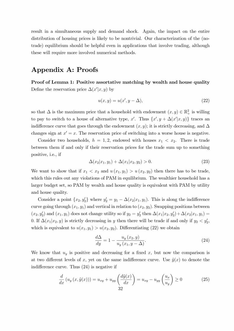
result in a simultaneous supply and demand shock. Again, the impact on the entire

distribution of housing prices is likely to be nontrivial. Our characterization of the (no-

trade) equilibrium should be helpful even in applications that involve trading, although

these will require more involved numerical methods.

Appendix A: Proofs

Proof of Lemma 1: Positive assortative matching by wealth and house quality

Define the reservation price ∆(0| ) by

( ) = (0 −∆) (22)

so that ∆ is the maximum price that a household with endowment ( ) ∈ R2+ is willingto pay to switch to a house of alternative type, 0. Thus {0 + ∆(0| )} traces anindifference curve that goes through the endowment ( ); it is strictly decreasing, and ∆

changes sign at 0 = The reservation price of switching into a worse house is negative.

Consider two households, = 1 2, endowed with houses 1 2. There is trade

between them if and only if their reservation prices for the trade sum up to something

positive, i.e., if

∆(2|1 1) +∆(1|2 2) 0. (23)

We want to show that if 1 2 and (1 1) (2 2) then there has to be trade,

which this rules out any violations of PAM in equilibrium. The wealthier household has a

larger budget set, so PAM by wealth and house quality is equivalent with PAM by utility

and house quality.

Consider a point {2 02} where 02 = 1 −∆(2|1 1). This is along the indifferencecurve going through (1 1) and vertical in relation to (2 2) Swapping positions between

(2 02) and (1 1) does not change utility so if 2 = 02 then ∆(1|2 02)+∆(2|1 1) =

0 If ∆(1|2 ) is strictly decreasing in then there will be trade if and only if 2 02,

which is equivalent to (1 1) (2 2). Differentiating (22) we obtain

∆

= 1− (2 )

(1 −∆). (24)

We know that is positive and decreasing for a fixed , but now the comparison is

at two different levels of , yet on the same indifference curve. Use () to denote the

indifference curve. Thus (24) is negative if

( ( ())) = +

µ()

¶= −

µ

¶≥ 0 (25)

32

This is just the condition for the marginal rate of substitution to be decreasing

in (i.e., for to be increasing in ), which holds for any quasi-concave utility

function.

Proof: Existence of equilibrium Let’s now discretize the house types, so that 0

0 · · · ∞. For brevity, we will refer to households endowed with a type- houseas households of type . Denote the mass of type- households with income equal or

lower than by (). We assume that all of these conditional income distributions are

continuous with full support [ ], where 0 ∞. The mass of type- householdsis 0, so

¡¢= . Recall that we have normalized the total mass at

P = 1.

With discretized house types we require an additional assumption:

(−1 ) ( ) for all = 1 (26)

This means that distribution of autarky utility has overlap between neighboring household

types. Together with Lemma 1, this implies that there must be trade between them, which

in turn will guarantee that price increments are uniquely determined.

Lemma 1 shows that equilibrium utility is increasing in the quality of the house con-

sumed. The full support of incomes and the overlap of autarky utilities imply that the

consumption levels of households that consume a house of type must be distributed

with full support on some interval [ ] ∈ [ ]. The unequivocally poorest and richest

households do not have anyone to trade with, so 0= and = .

The wealthiest household that consumes a type− house must be indifferent betweentrading up to the next house type. This indifference condition defines the price increments

∆ = − −1 as functions of upper bounds ,

(| +1) = {∆+1 : ( ) = (+1 −∆+1)} for all = 0 −1. (27)

Note that is single-valued for all ∈ [ ], with image in (0 ).The same indifference conditions can also be described in terms of the lower bounds

of the consumption intervals, with ( +1 +∆+1) = (+1 +1), so

+1

= −∆+1 = − (| +1) . (28)

Thus the lower bounds as well as the price increments are uniquely determined by the

upper bounds, so the equilibrium allocation can be described in terms of the alone,

where = 0 − 1.1919Equivalently, the allocation can be described in terms of the lower bounds

or prices ∆, where

= 1 . This choice of independent variables is a matter of convenience.

33

Demand for type- houses is the sum of demands from each household type. Consider

type− households endowed with income . They will consume a type- house if theirwealth is in the same range as of those type− households who consume their endowment: + ∈ [ +

+ ] The bounding inequalities for these intervals can be written as

≤ + −

≥ + − = −1 + −1 − (29)

for = 1 . (Recall that = .) Total demand for type− houses is

() =

X=0

[ ( + − )− (−1 + −1 − )] (30)

=

−1X=0

[ ( + (∆+1 + · · ·+∆))− (−1 + (∆+1 + · · ·+∆−1))]

+ ()− (−1 −∆)

+

X=+1

[ ( − (∆+1 + · · ·+∆))− (−1 − (∆ + · · ·+∆))] , (31)

where ∆ are functions of as defined by (27) and (28). Define the excess demand

functions as

() = max {0 ()}−, (32)

where the infeasible negative demands allowed by (30) are removed. The nonnegativity

constraint is binding if the upper bound is below the lower bound implied by −1.

Each household has zero net demand for housing units, because not trading amounts

to demanding your own house. Thus () = −P−1

=0 () and market equilibrium

can be defined as

() = 0 for = 0 − 1, (33)

or, in vector form, () = 0. This is a system of equations in unknowns.

Consider the best response of an imaginary "player" who attempts to minimize the

absolute value of excess demand for type− houses with the sole instrument of choosingthe upper bound . (The top house type, where = by construction, does not have

a "player" representing it.) Use − to denote the vector without the :th element. The

best response function is

(−) = arg min∈[]

| (|−)| . (34)

34

It is straightforward to show that is continuous and increasing in , but there may be

a flat region. This happens when is below the lower bound determined by −. Then

demand for −type houses is zero, and (|−) = −. However, the highest possible

lower bound is strictly below , by (28) it is − ¡|−1

¢, so must be strictly

increasing in some interval [ ]. There are two possibilities

(−) =

(

¡|−

¢ ≤ 0 (|−) = 0

, (35)

where ∈ ( ). Thus is single-valued but may not be able to eliminate excess supplyfor . Hence () = (0 (−0) −1

¡−(−1)

¢) defines a continuous vector-valued

function from [ ] to itself. Thus, by Brouwer Fixed Point theorem, there exists a fixed

point ∗ = (∗).

Next we prove, by contradiction, that a fixed point must be a market equilibrium.

Suppose that ∗ = (∗) but (∗) 0 for some , so ∗ = Now consider the

highest such , so that (∗) = 0 for all higher types ∈ { + 1 − 1}. Since

+1

= − ¡| +1¢ (due to overlap of autarky utilities) at least some +1-types

are trading down, while no one among types or lower is trading up to houses above .

Hence 0 for at least one , a contradiction with (35). Intuitively, all demand for

houses +1 and higher would have to come from households endowed with those houses.

Since some of them are trading down, there must be excess demand for some .

Thus any fixed point of indeed defines an equilibrium allocation of our model.

Finally, since is strictly increasing, the equilibrium allocation is associated with unique

price increments ∆, so associated equilibrium prices are unique up to an additive

constant. (However, we have not shown that there is a unique equilibrium allocation).

Appendix B: Data and preference inference

We use income and house price data from the American Housing Survey (AHS). House

price is based on the survey question where respondents were asked to estimate the current

market value of their house. We consider only homeowners, which amounts to assuming

that rental housing forms an entirely separate market.

The choice of MAs was determined by the availability of data. The most populous

MAs are covered only in national-level data (the National Surveys), where house prices are

top coded at a common national threshold. This results in a disproportionate censoring of

observations in the largest MAs. In those MAs where the national data is not decimated

by top coding it suffers from small sample size, which unfortunately renders the national

35

surveys useless for our purposes. Mid-size cities are covered in separate "Metro surveys,"

which have been conducted at irregular intervals and which are less affected by the top-

coding problem because they are done at city-level. Our sample includes all MAs from

which there is metro survey data both in 2007 (the most recent year) and 1998 (the second

most recent year for the MAs surveyed in 2007). Table B1 provides information about

the number of observations, inequality, the rank correlation between income and house

value, and population growth.

#Obs Gini Gini Gini Rank corr. Pop.

perm. income income house value growth %

1998 2007 1998 2007 1998 2007 1998 2007 1998 2007

Baltimore 2306 1211 0.16 0.17 0.37 0.40 0.27 0.28 0.38 0.48 6.2

Boston 1960 1075 0.13 0.17 0.36 0.44 0.25 0.23 0.48 0.46 3.7

Houston 1963 1105 0.18 0.20 0.39 0.41 0.30 0.27 0.53 0.52 26.1

Minneapolis 2741 1524 0.14 0.16 0.33 0.36 0.23 0.23 0.50 0.49 10.5

Tampa 2106 1255 0.19 0.23 0.41 0.52 0.29 0.31 0.52 0.48 16.2

Washington 2356 1315 0.14 0.17 0.33 0.39 0.25 0.23 0.50 0.49 16.4

Table B1. Number of observations, summary statistics for inequality (Gini coeffi-

cient) of permanent income, income, and house value, and for the Spearman rank corre-

lation between income and house value, and population growth from 2000 to 2010 according

to Census data. "Permanent income" is income kernel smoothed relative to house price.

Figure 7 shows the relative prediction errors, log(0707), by quantile of house value

for the three MAs where the population has grown the least from 2000 to 2010. The

solid lines show the prediction errors given the MA specific elasticity of substitution that

minimizes the mean absolute percentage error (MAPE) in each MA. The elasticities are

0.42, 0.63, and 0.48 for Baltimore, Boston and Minneapolis, respectively. The resulting

MAPEs are 4.6% (Baltimore), 2.8% (Boston),and 2.6%.(Minneapolis). The model seems

to provide a reasonable fit, especially in Boston and Minneapolis. The dashed lines show

the prediction errors given our baseline assumption of an elasticity of substitution equal

to 0.5.

36

0 0.5 1−30

−20

−10

0

10

20

30

Relat

ive er

ror, %

Baltimore

0 0.5 1−30

−20

−10

0

10

20

30Boston

Price quantile0 0.5 1

−30

−20

−10

0

10

20

30Minneapolis

Figure 7: Errors in predicted 2007 house prices.

References

Alonso, William (1964). Location and Land Use. Harvard University Press, Cam-

bridge, MA.

Bajari, Patrick; Chan, Phoebe; Krueger, Dirk and Daniel Miller (2010).

A Dynamic Model of Housing Demand: Estimation and Policy Implications. NBER

Working Paper 15955.

Braid, Ralph M (1981). “The Short-Run Comparative Statics of a Rental Housing

Market.” Journal of Urban Economics, 10, pp. 286-310.

Caplin, Andrew and John Leahy (2010). “A Graph Theoretic Approach to

Markets for Indivisible Goods.” NBER Working Paper 16284.

Davis, Morris and Jonathan Heathcote (2007). “The Price and Quantity of

Residential Land in the United States.” Journal of Monetary Economics, 54, pp. 2595—

2620.

Davis, Morris and Michael Palumbo (2008). “The Price of Residentical Land

in Large US Cities.” Journal of Urban Economics, 63, pp. 352—384.

Diamond, Rebecca (2012). “The Determinants and Welfare Implications of US

Workers’ Diverging Location Choices by Skill:1980-2000.” Harvard mimeo.

Eeckhout, Jan; Roberto Pinheiro, and Kurt Schmidheiny (2013): “Spatial

Sorting.” Working paper.

Epple, Dennis and Holger Sieg (1999). “Estimating EquilibriumModels of Local

Jurisdictions.” Journal of Political Economy, 107(4), pp. 645—681.

37

Fujita, Masahisa (1989). Urban Economic Theory: Land Use and City Size. Cam-

bridge University Press, Cambridge, UK.

Gale, David (1984). “Equilibrium in a Discrete Exchange Economy with Money.”

International Journal of Game Theory, 13(1), pp. 61—64.

Glazer, Amihai; Vesa Kanniainen and Panu Poutvaara (2008). “Income

Taxes, Property Values, and Migration.” Journal of Public Economics, 92, pp. 915—923.

Gyourko, Joseph; Christopher Mayer and Todd Sinai (2006). “Superstar

Cities.” NBER Working Paper 12355.

Landvoigt, Tim; Monika Piazzesi and Martin Schneider (2012). “The Hous-

ing Market(s) of San Diego.” NBER Working Paper 17723.

Legros, Patrick and Andrew F Newman (2007). “Beauty Is a Beast, Frog

Is a Prince: Assortative Matching with Nontransferabilities.” Econometrica, 75(4), pp.

1073-1102.

Li, Wenli; Haiyoung Liu and Rui Yao (2009). “Housing over Time and over

the Life Cycle: A Structural Estimation.” Federal Reserve Bank of Philadelphia Working

Paper.

Määttänen, Niku and Marko Terviö (2009). “Income Distribution and Housing

Prices: An Assignment Model Approach.” HSE Working Paper.

Moretti, Enrico (2013). “Real Wage Inequality.” American Economic Journal:

Applied Economics, 5(1), pp. 65-103.

Ortalo-Magné, François and Sven Rady (2006). “Housing Market Dynamics:

On the Contribution of Income Shocks and Credit Constraints.” Review of Economic

Studies, 73, pp. 459-85.

Ortalo-Magné, François and Andrea Prat (2010). “Spatial Asset Pricing: A

First Step.” Working paper.

Quinzii, Martine (1984). “Core and Competitive Equilibria with Indivisibilities.”

International Journal of Game Theory, 13(1), pp. 41—60.

Ríos-Rull, José-Victor and Virginia Sanchez-Marcos (2008): “An Aggre-

gate Economy with Different House Sizes.” Journal of The European Economic Associa-

tion, P&P, 6(2-3), pp. 705-14.

Sattinger, Michael (1979). “Differential Rents and the Distribution of Earnings.”

Oxford Economic Papers, 31, pp. 60-71.

Sattinger, Michael (1993). “Assignment Models of the Distribution of Earnings.”

Journal of Economic Literature, 31, pp. 831-880.

Shapley, Lloyd and Herbert Scarf (1974). “On Cores and Indivisibility.” Jour-

nal of Mathematical Economics, 1(1), pp. 23—27.

38

Terviö, Marko (2008). “The Difference that CEOs Make: An Assignment Model

Approach.” American Economic Review 98(3), pp. 642—668.

Teulings, Coen N (1995). “The Wage Distribution in a Model of the Assignment

of Skills to Jobs.” Journal of Political Economy, 102, pp. 280—315.“

Tiebout, Charles M (1956). A Pure Theory of Local Expenditure.” Journal of

Political Economy, 64, pp. 416—424.

Van Nieuwerburgh, Stijn and Pierre-Olivier Weill (2010). “Why Has House

Price Dispersion Gone Up?” Review of Economic Studies, 77(4), pp.1567—1606.

39