Incentivized actions in freemium games1

Mahesh Nagarajan∗ Christopher Thomas Ryan† Lifei Sheng‡

Yuan Cheng § Chunyang Tong¶2

April 13, 20183

Abstract4

We explore the phenomena of game companies offering to pay users in “virtual” benefits5

to take actions in-game that earn the game company revenue from third parties. Examples of6

such “incentivized actions” include paying users in “gold coins” to watch video advertising or7

speeding in-game progression in exchange for filling out a survey. These are common practices8

in mobile games that use a freemium business model, where users download and play for free9

and only a relatively small percentage of total users pay out-of-pocket when playing the game.10

We develop a dynamic optimization model that looks at the costs and benefits of offering11

incentivized actions to users as they progress in their engagement with the game. We find12

sufficient conditions for the optimality of a threshold strategy of offering incentivized actions to13

low-engagement users and then removing incentivized actions to encourage real-money purchases14

once a player is sufficiently engaged. Our model also provides insights into what types of games15

can most benefit from offering incentivized actions. For instance, our analysis suggests that16

social games with strong network effects have more to gain from offering incentivized actions17

than solitary games.18

1 Introduction19

Games represent the fastest growing sector of the entertainment industry globally, which includes20

music, movies, and print publishing (McKinsey, 2013). Moreover, the online/mobile space is the21

fastest growing segment of games, which is itself dominated by games employing a “freemium” busi-22

ness model. Freemium games are free to download and play and earn revenue through advertising23

or selling game enhancements to dedicated players. When accessed on 23 April 2015, Apple Inc.’s24

App Store showed 190 out of the 200 top revenue-generating games (and all of the top 20) were25

free to download.1 On Google Play, the other major mobile games platform, 297 out of the 300 top26

revenue-generating games were freemium.2 Moreover, games are the dominant revenue generators27

∗Sauder School of Business, University of British Columbia, E-mail: mahesh.nagarajan@sauder.ubc.ca†Booth School of Business, University of Chicago, E-mail: chris.ryan@chicagobooth.edu‡College of Business, University of Houston-Clear Lake, E-mail: fay.sheng@sauder.ubc.ca§School of Economics and Management, Tsinghua University, E-mail: chengyn@sem.tsinghua.edu.cn¶Shanghai University of Finance and Economics

1

in the global app market. Revenue from mobile games accounts for 79 percent of total app revenue28

on Apple’s App Store and 92 percent of revenue on Google Play.329

The concept behind freemium is to attract large pools of players, many of whom might never30

make an in-app purchase. Players that do pay out of pocket are said to monetize. In general,31

successful games have a monetization rate of between 2 and 10 percent, with the average much32

closer to 2 percent.4 When game publishers cannot earn directly from the pockets of consumers,33

they turn to other sources of revenue. This is largely through third parties who pay for delivering34

advertising content and having players download other apps, fill out surveys or apply for services,35

such as credit cards. This stream of revenue is less lucrative per conversion than in-app purchases.36

Typically, delivering a video earns pennies on the dollar compared to in-app purchases.37

However, players can become irritated by advertising, especially when it interrupts the flow or38

breaks the fiction of a game. A recent innovation is to offer “incentives” for players to click on a39

banner ad, watch a video or fill out a survey. These are collectively called incentivized actions, or40

as it is commonly shortened, incented actions. To get a clearer sense of how incented actions work41

we examine a concrete example.42

Candy Crush Saga is a puzzle game, published by King. King was recently acquired by43

Activision-Blizzard for 5.9 billion USD based on the enduring popularity of Candy Crush Saga44

and its portfolio of successful games.5 In Candy Crush Saga, a player attempts to solve a progres-45

sion of increasingly challenging puzzles. At the higher levels, players get stuck for extended periods46

on a single puzzle. Player progression is further hindered by a “lives” mechanic where each failed47

attempt at a puzzle consumes one of at most five total lives. Lives are regenerated either through48

waiting long periods of real-time or by purchasing additional lives with real money. Players may49

also buy items that enhance their chances of completing a puzzle.50

Early versions of Candy Crush Saga had incented actions, including advertising. A player could51

take an incented actions to earn lives or items without using real money. However, in June of 2013,52

six months after Candy Crush Saga was launched on Apple iOS, King decided to drop all forms of53

in-game advertising in the game.6 King’s choice was surprising to many observers. What was the54

logic for removing a potential revenue stream? How did this move affect the monetization rate?55

This raises other more tactical questions: when in the lifetime of a player is it best to offer56

incented actions? Should some players be offered incented actions and others not? Finally, there57

are related strategic questions: what types of games are best suited to offering incented actions?58

In this paper, we present an analytical model to explore the use of incented actions and attempt59

to answer the above questions. In particular, we are interested in a game publisher’s decision of60

when to offer incented actions to players, and when to remove this option. Our model emphasizes61

the connection of incented actions to two other useful concepts often discussed in the game industry62

– engagement and retention. Highly engaged players are more likely to make in-app purchases and63

less likely to quit. The longer a player is retained in the game, the more likely they are to become64

engaged and monetize. Analytically, player engagement levels are modeled as states in a Markov65

2

chain and retention is the time a player stays in the system before being absorbed into a “quit”66

state. The more engaged a player, the more likely they are retained.67

The concept of engagement is common to both games industry practitioners and academics who68

study the video game industry. Although all observers emphasize the importance of measuring69

player engagement, there is little consensus on how to measure it. Among practitioners (see, for70

instance, Lovell (2012)) a common measurement is the ratio of daily active users (DAU) over71

monthly active users (MAU). DAU measures the average number of users who play the game at72

least once per day, and MAU measures the average number of users who play the game at least73

once per month. This aggregate measure says relatively little about the behavior of an individual74

player. However, it is easy to calculate for publicly traded games companies that typically publish75

their DAU and MAU numbers and thus can be used as a benchmark. It also has the virtue of being76

universal across many game designs where the mechanics of the game (being a puzzle, sports or77

adventure game) may otherwise have little in common.78

There is also substantial research on engagement in academic video game development jour-79

nals. A recent study by Abbasi et al. (2017) describes a variety of quantitative and qualitative80

measurements of engagement including notions of immersion, flow, presence, etc. These are typi-81

cally measured via questionnaires (such as the game-experience questionnaire (GEQ) proposed in82

Jennett et al. (2008)). This notion of engagement focuses on the psychological and cognitive state83

of the player and thus presents challenges to operationalize from the game designer’s perspective.84

Another view of engagement connects to notions of progress made by the player in the game.85

Players can invest significant time and resources to reach higher “levels” of progression. It can86

be difficult for players to walk away from playing a game they have heavily invested in. Thus, a87

simple measure of engagement is the extent to which a player has invested her energy in a game. In88

discussions with game developers, the primary focus of game design is to improve retention, with89

the empirically well-founded belief that the longer the relationship a player has with a game, the90

greater their willingness to spend.7 The association of engagement with levels has the benefit of91

having both a psychological component and also be based on measurable game data. Progression92

suggests an investment of time and achievement of mastery that correlate well with psychological93

notions of engagement. On the other hand, progression can often be directly measured. For games94

like Candy Crush Saga, there are concrete and distinct levels that are reached by the player. In95

Candy Crush Saga, the current level is the number of puzzles completed by the player.96

Not every game has a clear level-based design. For such games, other measures of engagement97

are typically employed. In Section 5 we analyze a proprietary data set for the game Survival of98

Primitive (or Primitive, for short) developed by Ebo games. This game has a less linear notion99

of progression than Candy Crush, where “survival” depends on a variety of resource collection100

activities with many possible paths towards success. In this setting, we abandon the “level”-based101

notion of engagement and adopt Ebo’s measure of engagement based on the duration of daily play.102

3

Our results. Our results come in two forms; first, analytical results based on a model with a103

level-based notion of engagement (inspire by Candy Crush Saga and second, a data-driven of the104

optimality of incented actions using our proprietary dataset for Primitive. Interestingly, both our105

analytical and numerical results share a common theme: an optimal deployment of incented actions106

(under a broad set of data specifications) is to offer incented actions to players with low engagement107

until they reach a threshold level of engagement, after which incented actions are removed. We108

also show how the optimal threshold level depends on changes in game parameters.109

Our analytical results depend on a careful analysis of three main effects of incented actions.110

These effects are described in with greater precision below, but we mention them here at a con-111

ceptual level. First is the revenue effect. By offering incented actions, game publishers open up112

another channel of revenue. However, the net revenue of offering incented may nonetheless be113

negative if one accounts for the opportunity costs of players not making in-app purchases. This114

captures the possibility that a player would have made an in-app purchase if an incented action was115

not available. Second, the retention effect measures how effective an incented action is at keeping116

players from quitting. In other words, incented actions can delay a player’s decision to quit the117

game. Third, the progression effect refers to the effectiveness of an incented action in deepening118

the engagement level of the player. It refers to an incented actions ability to increase the player’s119

attachment to the game. These three effects are intuitively understood by game developers and120

the topic of much discussion and debate in the gaming industry.121

Gaming companies grapple with the issue of understanding how these effects interact with each122

other in the context of specific games. As we shall see in concrete examples below, all three effects123

can act to either improve or erode the overall revenue available to the publisher. Each effect is124

connected and often move in similar directions as players progress. Part of our analysis is to describe125

situations where the effects move in different, sometimes counter-intuitive, directions.126

We can analytically characterize each effect, allowing us to gain insights into how to optimally127

design a policy for offering incented actions. To understand the interactions between these effects128

and to capture the dynamics in a game, we use Markov chains to model player engagement and129

how they transition from one level of engagement to another. Then, using a Markov Decision130

Process (MDP) model we study the effect of specific decisions or policies of the game publisher.131

For example, we provide sufficient conditions for when a threshold policy is optimal. In a threshold132

policy incented actions are offered until a player reaches a target engagement level, after which133

incented actions are removed. The intuition of these policies is clear. By offering incented actions,134

the retention effect and progression effect keep the player in for longer by providing a non-monetizing135

option for progression. However, once a player is sufficiently engaged, the revenue effect becomes136

less beneficial and the retention effect less significant because highly engaged players are more likely137

to buy in-app purchases and keep playing the game. This suggests that it is optimal to remove138

incented actions and attempt to extract revenue directly from the player through monetization.139

Our sufficient conditions justify this logic, but we also explore settings where this basic intuition140

4

breaks down. For instance, it is possible that the retention effect remains a dominant concern even141

at higher engagement levels. Indeed, a highly engaged player may be quite likely to monetize, and142

so there is a strong desire on the part of the publisher to keep the player in the system for longer143

by offering incented actions to bolster retention.144

The relative strengths of these three effects depend on the characteristics the game, including145

all the parameters in our MDP model. We examine this dependence by tracking how the threshold146

in an optimal threshold policy changes with the parameters. This analysis provides insights into147

the nature of optimal incented action policies.148

For instance, we show analytically that the more able players are at attracting their friends into149

playing the game, the greater should be the threshold for offering incented actions. This suggests150

that social games that include player interaction as part of their design should offer incented actions151

more broadly, particularly when the retention effect is strongly positive since keeping players in the152

game for longer gives them more opportunities to invite friends. Indeed, a common incented action153

is to contact friends in your social network or to build a social network to earn in-game rewards.154

This managerial insight can assist game publishers in targeting what types of games in a portfolio155

of game projects can take the most advantage of delivering incented actions.156

We also discuss different effects of the design of incented actions, in particular, their “strength”157

at attracting and engaging players. “Strength” here refers to how powerful the reward of the158

incented action is in the game. For instance, this could be the number of “coins” given to the159

player when an incented action is taken. If this reward is powerful, in comparison to in-app160

purchases, then it can help players progress, strengthening the progression effect. On the other161

hand, a stronger incented action may dissuade players further from monetizing, strengthening162

cannibalization. Through numerical examples, we illustrate a variety of possible effects that tradeoff163

the behavioral effects of players responding to the nature of the incented action reward and show164

that whether or not to offer incented actions to highly engaged players depends in a nonmonotonic165

way on the parameters of our model that indicate the strength of incented actions.166

Finally, we analyze the data we gathered on Survival of Primitive from our industry partner.167

This game does not fully fit the main analytical setting explored in the previous settings because168

Primitive does not have a level-based design. Nonetheless, we use this data to calibrate a Markov169

Decision process to compute optimal policies. Interestingly, the optimality of threshold policies170

persists under almost all of our simulated values for parameters we could not clearly define using171

the provided data. Moreover, the sensitivity of the threshold to changes in various game parameters172

also follows the pattern predicted by our analytical results. Another way to interpret these findings173

is that the main intuition of our analytical findings is supported by a robustness check using data174

from a real game that satisfy a more general set of assumptions. Much of this was shared with175

our partner and the main insights from our analysis guided a their subsequent data collection and176

design policies.177

5

2 Related literature178

As freemium business models have grown in prominence, so has interest in studying various aspects179

of freemium in the management literature. While papers in the marketing literature on freemium180

business models has been largely empirical (see for instance Gupta et al. (2009) and Lee et al.181

(2017)), our work connects most directly to a stream of analytical studies in the information182

systems literature that explores how “free” is used in the software industry. Two important papers183

for our context are Niculescu and Wu (2014) and Cheng et al. (2015) that together establish a184

taxonomy of different freemium strategies and examine in what situations a given strategy is most185

advantageous. Seeding is a strategy where some are given away entirely for free, to build a user base186

that attracts new users through word-of-mouth and network effects. Previous studies explored the187

seeding strategy by adapting the Bass model (Bass, 1969) to the software setting (see for instance188

Jiang and Sarkar (2009)). Another strategy is time-limited freemium where all users are given access189

to a complete product for a limited time, after which access is restricted (see Cheng and Liu (2012)190

for more details). The feature-limited freemium category best fits our setting, where a functional191

base product can always be accessed by users, with additional features available for purchase by192

users. In freemium mobile games, a base game is available freely for download with additional193

items and features for sale through accumulated virtual currency or real-money purchases.194

Our work departs from this established literature in at least two dimensions. First, we focus195

on how to tactically implement a freemium strategy, in particular, when and how to offer incented196

actions to drive player retention and monetization. By contrast, the existing literature has largely197

focused on comparing different freemium strategies and their advantage over conventional software198

sales. This previous work is, of course, essential to understanding the business case for freemium.199

Our work contributes to a layer of tactical questions of interest to firms committed to a freemium200

strategy in search of additional insights into its deployment.201

Second, games present a specific context that may be at odds with some common conceptualiza-202

tions of a freemium software product. For a productivity-focused product, such as a PDF editor, a203

typical implementation of freemium is to put certain advanced features behind a pay-wall, such as204

the ability to make handwritten edits on files using a stylus. Once purchased, features are typically205

unlocked either in perpetuity or for a fixed duration by the paying player. By contrast, virtual206

items or currency that may enhance the in-game experience, speed progression, or provide some207

competitive advantage are typically purchased in games. These purchases are often consumables,208

meaning that they are depleted through use. This is true, for instance, of all purchases in Candy209

Crush Saga. Our model allows for a player to make repeated purchases and the degree of intensity210

of monetization to evolve over the course of play.211

Other researchers have examined the specific context offered by games, as opposed to general212

software products, and have adapted specialized theory to this specific context. Guo et al. (2016)213

examine how the sale of virtual currencies in digital games can create a win-win scenario for players214

6

and publishers from a social welfare perspective. They make a strong case for the value created215

by games offering virtual currency systems. Our work adds a layer by examining how virtual216

currencies can be used to incentivize players to take actions that are profitable to the firm that217

does not involve a real-money exchange. A third-party, such as an advertiser, can create a mutually218

beneficial situation where the player earns additional virtual currency, the publisher earns revenue219

from the advertiser, and the advertiser promotes their product. Also, Guo et al. (2016) develop a220

static model where players decide on how to allocate a budget between play and purchasing virtual221

currency. We relate a player’s willingness to take incented actions or monetize as their engagement222

with the game evolves, necessitating the use of a dynamic model. This allows us to explore how a223

freemium design can respond to the actions of players over time. This idea of progression in games224

has been explored empirically in Albuquerque and Nevskaya (2012). We adapt similar notions to225

derive analytical insights in our setting.226

The dynamic nature of our model also shares similarities with threads of the vast customer227

relationship management (CRM) literature in marketing. In this literature, researchers are inter-228

ested in how firms balance acquisition, retention, and monetization of players through the pricing229

and design of their product or service over time. For example, Libai et al. (2009) adapt Bass’s230

model to the diffusion of services where player retention is an essential ingredient in the spread231

of the popularity of a platform. Fruchter and Sigue (2013) provide insight into how a service232

can be priced to maximize revenue over its lifespan. Both studies employ continuous-time and233

continuous-state models that are well-suited to examine the overall flow of player population. Our234

focus of analysis is at the player level and asks how to design the game (i.e., service) to balance235

retention and monetization through offering incented actions for a given acquired player. Indeed,236

game designs on mobile platforms can, in principle, be specialized down to a specific player. With237

the increasing availability of individual player level data, examination of how to tailor design with238

more granularity is worthy of exploration. By contrast, existing continuous models treat a single239

player’s choice with measure zero significance.240

Finally, our modeling approach of using a discrete time Markov decision process model in search241

of threshold policies is a standard-bearer of analysis in the operations management literature.242

We have mentioned the advantages of this approach earlier. Threshold policies, which we work243

to establish, have the benefit of being easily implementable and thus draw favor in studies of244

tactical decision-making that is common in multiple areas including the economics and operations245

management literature. The intuition for their ease of use is somewhat easy to understand. The246

simplest type of threshold policies allows the system designer to simply keep track of nothing but247

the threshold (target) level and monitor the state of the system and take the appropriate action248

to reap the benefits of optimality. This is in contrast to situations where the optimal policy can249

be complex and has nontrivial state and parameter dependencies. Examples of effective use of250

this approach in dynamic settings include inventory and capacity management and control (Zipkin,251

2000) and revenue management (Talluri and Van Ryzin, 2006).252

7

3 Model253

We take the perspective of a game publisher who is deciding how to optimally deploy incented254

actions. Incented actions can be offered (or not) at different times during a player’s experience255

with the game. For example, a novice player may be able to watch video ads for rewards during256

the first few hours of gameplay, only later to have this option removed.257

Our model has two agents: the game publisher and a single player. This assumes that the game258

publisher can offer a customized policy to each player, or at least customized policies to different259

classes of players. In other words, the “player” in our model can be seen as the representative of a260

class of players who behave similarly. The publisher may need to decide on several different policies261

for different classes of players for an overall optimal design.262

We assume that the player behaves stochastically according to the options presented to her by263

the game publisher. The player model is a Markov chain with engagement level as the state variable.264

The hope is that this model will allow for many personal interpretations of what “engagement”265

specifically means. We do not model down to the specifics of a particular game and instead provide266

what we feel is a robust approach to engagement. The game publisher’s decision problem is a267

Markov Decision Problem (MDP) where the stochasticity is a function of the underlying player268

model, and the publisher’s decision is whether or not to offer incented actions. The player model269

is described in detail in the next subsection. The publisher’s problem is detailed in Section 3.2.270

3.1 Player model. The player can take three actions while playing the game. The first is to271

monetize (denoted M) by making an in-app purchase with real money. The second is to quit272

(denoted Q). Once a player takes the quit action, she never returns to playing the game. Third,273

the player can take an incented action (denoted I). The set of available actions is determined by274

whether the publisher offers an incented action or not. We let A1 = {M, I,Q} denote the set of275

available actions when an incented action is offered and A0 = {M,Q} otherwise.276

The probability that the player takes a particular action depends on her engagement level (or277

simply level). These levels form the states of the Markov Chain. The set E of engagement levels278

is a discrete set (possibly countable), while −1 denotes a “quit” state where the player no longer279

plays the game. That is, the quit state is an absorbing state. The probability that the player takes280

a particular action also depends on what actions are available to her. We used the letter “p” to281

denote probabilities when an incented action is available and write pa(e) to denote the probability282

of taking action a ∈ A1 at level e ∈ E. For example, pM (2) is the probability of monetizing at283

level 2 while pI(0) is the probability of taking an incented action at level 0. We use the letter284

“q” to denote action probabilities when the incented action is unavailable and write qa(e) for the285

probability of taking action a ∈ A0 at level e ∈ E. By definition pM (e) + pI(e) + pQ(e) = 1 and286

qM (e) + qQ(e) = 1 for all e ∈ E.287

There is a relationship between pa(e) and qa(e). When an incentivized action is not available288

the probability pI(e) is allocated to the remaining two actions M and Q. For each e ∈ E we assume289

8

that there exists a parameter α(e) ∈ [0, 1] such that:290

qM (e) = pM (e) + α(e)pI(e) (1)291

qQ(e) = pQ(e) + (1− α(e))pI(e). (2)292293

We call α(e) the cannibalization parameter at level e, since α(e) measures the impact of remov-294

ing an incented action on the probability of monetizing and thus captures the degree to which295

incented actions cannibalize demand for in-app purchases. A large α(e) (close to 1) implies strong296

cannibalization whereas a small α(e) (close to 0) signifies weak cannibalization.297

It remains to consider how a player transitions from one level to another. We must first describe298

the time epochs where actions and transitions take place. The decision epochs where actions are299

undertaken occur when the player is assessing whether or not they want to continue playing the300

game. The real elapsed time between decision epochs is not constant since it depends on the301

behavior of the player between sessions of play. Some players frequently play, others play only for302

a few minutes per day. A player might be highly engaged but have little time to play due to other303

life obligations. This reality suggests that the elapsed time between decision epochs should not304

be a critical factor in our model. We denote the level at decision epoch t by et and the action at305

decision epoch t by at.306

Returning to the question of transitioning from level to level, in principle we would need to307

determine individually each transition probability P(et+1 = e′|et = e and at = a). For actions308

a ∈ {M, I}, we will assume that transition probabilities are stationary and set P(et+1 = e′|et =309

e and at = a) = τa(e′|e) for all times t, where τ is a [0, 1]-valued function such that

∑e′∈E τa(e

′|a) =310

1 for all e ∈ E and a ∈ {M, I}. For the quit action, P(et+1 = −1|et = e′ and at = Q) = 1 for all311

times t and engagement levels e′. In other words, there are no “failed attempts” at quitting.312

Taken together we get aggregate transition probabilities from state to state, depending on313

whether incented ads are available or not. If incented ads are available, the transition probability314

from engagement level e to engagement level e′ is315

P1(e′|e) :=

pM (e)τ(e′|e,M) + pI(e)τ(e′|e, I) if e, e′ ∈ EpQ(e) if e ∈ E, e = −1

1 if e, e′ = −1

0 otherwise,

(3)316

317

and if incented ads are not available318

P1(e′|e) :=

qM (e)τ(e′|e,M) if e, e′ ∈ EqQ(e) if e ∈ E, e = −1

1 if e, e′ = −1

0 otherwise,

(4)319

320

Assumption 1. No matter how engaged, there is always a positive probability that a player will321

9

quit; i.e., pQ(e), qQ(e) > 0 for all e ∈ E.322

This acknowledges the fact that games are entertainment activities, and there are numerous323

reasons for a player to quit due to factors in their daily lives, even when engrossed in the game.324

This is also an important technical assumption since it implies the publisher’s problem (see the325

next section) is an absorbing Markov decision process.326

3.2 The publisher’s problem. We model the publisher’s problem as an infinite horizon Markov327

decision process under a total reward criterion (for details see Puterman (1994)). A Markov decision328

process is specified by a set of states, controls in each state, transition probabilities under pairs of329

states and controls, and rewards for each transition.330

Specifically in our setting based on the description of the dynamics we have laid out thus far,331

the set of states is {−1} ∪ E and the set of controls U = {0, 1} is independent of the state, where332

1 represents offering an incented action and 0 not offering an incented action. The transition333

probabilities are given by (3) when u = 1 and (4) when u = 0. The reward depends on the action334

of the player. When the player quits, the publisher earns no revenue, denoted by µQ = 0. When335

the player takes an incented action, the publisher earns µI , while a monetization action earns µM .336

Assumption 2. We assume µI < µM .337

This assumption is in concert with practice, as discussed in the introduction.338

The expected reward in state e under control u is:339

r(e, u) =

pM (e)µM + pI(e)µI if e ∈ E and u = 1

qM (e)µM if e ∈ E and u = 0

0 if e = −1.

340

341

Note that expected rewards do not depend on whether the player transitions to a higher level and342

so the probabilities τa(e′|e) do not appear in r(e, u).343

A policy y for the publisher is a mapping from E to U . On occasion we will express a policy344

by the vector form of its image. That is, the vector y = (1, 0, 1) denotes offering incented actions345

in engagement levels 1 and 3. Each policy y induces a stochastic process over rewards, allowing us346

to write its value as:347

W y(e) := Eye

[ ∞∑t=1

r(et, y(et))

](5)348

349

where e is the player’s initial level, and the expectation Eye [·] derives from the induced stochastic350

process. One may assume that all players start at level 0, but we also consider the possibility that351

players can start at higher levels of the game for a couple of reasons. First, the time horizon of the352

available may only capture the situation where some existing players have already started playing353

the game. Second, we reason inductively where it is valuable to think of the process of restarting354

at a higher level. For these reasons we allow the initial level of the player to be different than 0.355

In many Markov decision processes, the sum in (5) does not converge, but under Assumption 1,356

10

the expected total reward converges for every policy y. In fact, our problem has a special structure357

that we can exploit to derive a convenient analytical form for (5) as follows:358

W y(e) =∑e′∈E

nye,e′r(e′, y(e′)) (6)359

360

where nye,e′ is the expected number of visits to engagement level e′ starting in engagement level e.361

We derive closed-form expressions for ne,e′ that facilitate analysis. For details see Appendix A.1.362

The game publisher chooses a policy to solve the optimization problem: given a starting en-363

gagement level e solve:364

maxy∈{0,1}E

W y(e). (7)365

366

This problem can be solved numerically using tools such as policy iteration (see, for instance,367

Puterman (1994)). These results are standard in the case of a finite number of engagement levels.368

The case of countably-many engagement levels also permits algorithms under additional conditions369

on the data (see, for instance, Hinderer and Waldmann (2005)). In our setting, rewards are bounded370

(equal to µI , µM or 0 for every e), which simplifies analysis. In this paper, we do not explore the371

countable engagement-level case.372

The challenge, of course, in solving (3.2) is fitting the data to the model. This is taken up later373

in Section 5 for a specific game of interest. For now, we aim to learn more about the analytical374

structure of optimal solutions to (3.2). In general, the situation is hopeless. Although the decision375

of the publisher is a simple {0, 1}-vector, the transition law (3)–(4) is quite general and evades the376

standard analysis needed to leverage existing structural results (such as monotonicity or submod-377

ularity). We consider a special case in the next section that will help us, nonetheless, get some378

structural insight into (7). In that setting we are able to show the optimality of threshold policies379

and conduct sensitivity analysis on the threshold level.380

Game companies can make use of our results in a number of ways. By numerically solving381

(3.2) using an approach similiar to our Section 5, a detailed policy for offering incented actions382

can be devised. However, even for new games with little user data to estimate the parameters of383

this optimization problem, structural results from the analytical model can provide guidance. Our384

results suggest it is quite justified to restrict to threshold policies, which are easy to understand385

for game designers and easy to implement in practice. Also, sensitivity analysis yields insights into386

what general types of games may want to include incented actions or not (see this discussion in387

Section 4.3).388

4 Analytical results for a special case389

To facilitate analysis, we make the following simplifying assumption about state transitions (these390

assumptions are relaxed in the data-driven Section 5 below): (i) players progress at most one391

level at a time and never digress, (ii) the transition probability is independent of the current level392

and depends only on the action taken by the player, and (iii) there are finitely many engagement393

11

0 1

M

I

-1pQ(0) qQ(1)

qM (1)

pI(0)

1− τI

1− τM

pM (0)

τM

τI

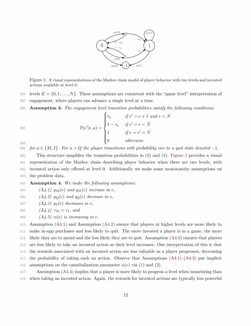
Figure 1: A visual representations of the Markov chain model of player behavior with two levels and incentedactions available at level 0.

levels E = {0, 1, . . . , N}. These assumptions are consistent with the “game level” interpretation of394

engagement, where players can advance a single level at a time.395

Assumption 3. The engagement level transition probabilities satisfy the following conditions:396

P(e′|e, a) =

τa if e′ = e+ 1 and e < N

1− τa if e′ = e < N

1 if e = e′ = N

0 otherwise

397

398

for a ∈ {M, I}. For a = Q the player transitions with probability one to a quit state denoted −1.399

This structure simplifies the transition probabilities in (3) and (4). Figure 1 provides a visual400

representation of the Markov chain describing player behavior when there are two levels, with401

incented action only offered at level 0. Additionally we make some monotoncity assumptions on402

the problem data.403

Assumption 4. We make the following assumptions:404

(A4.1) pM (e) and qM (e) increase in e,405

(A4.2) pQ(e) and qQ(e) decrease in e,406

(A4.3) pI(e) decreases in e,407

(A4.4) τM > τI , and408

(A4.5) α(e) is increasing in e.409

Assumption (A4.1) and Assumption (A4.2) ensure that players at higher levels are more likely to410

make in-app purchases and less likely to quit. The more invested a player is in a game, the more411

likely they are to spend and the less likely they are to quit. Assumption (A4.3) ensures that players412

are less likely to take an incented action as their level increases. One interpretation of this is that413

the rewards associated with an incented action are less valuable as a player progresses, decreasing414

the probability of taking such an action. Observe that Assumptions (A4.1)–(A4.3) put implicit415

assumptions on the cannibalization parameter α(e) via (1) and (2).416

Assumption (A4.4) implies that a player is more likely to progress a level when monetizing than417

when taking an incented action. Again, the rewards for incented actions are typically less powerful418

12

than what can be purchased for real money and so monetizing more likely leads to an increase419

in level. The example in games such as Crossy Road (by Hipster Whale), playable characters in420

the game can be directly bought with real money, but watching video ads can only contributes to421

random draws for characters.422

Finally, (A4.5) implies that a greater share of the probability of taking an incented actions when423

offered is allocated to monetization when an incented ad is removed (see (1)). As a player moves424

higher up in levels, the monetization option becomes relatively more attractive than quitting once425

the incented action is removed. Indeed, quitting has the player walking away from a potentially426

significant investment of time and mastery captured by a high level in the game.427

4.1 Understanding the effects of incented actions. In this section, we show how our analyt-428

ical model under our additional assumptions helps sharpen our insight into the costs and benefits429

of offering incented actions in games. In particular, we give precise analytical definitions of the430

revenue, retention and progression effects discussed in the introduction.431

Let y1e be a given policy with y1

e(e) = 0 for some engagement level e. Consider a local change to432

a new policy y2e where y2

e(e) = 1 but y2e(e) = y1

e(e) for e 6= e. We call y1e and y2

e paired policies with433

a local change at e. Analyzing this local change at the target engagement level e gives insight into434

the effect of starting to offer an incented action at a given engagement level. Moreover, this flavor435

of analysis suffices to determine an optimal threshold policy, as discussed in Section 4.2 below. For436

ease of notation, let W 1(e) = W y1e (e) and W 2(e) = W y2

e (e).437

Our goal is to understand the change in expected revenue moving from policy y1e to policy y2

e438

where the player starts (or has reached) engagement level e. Indeed, because the engagement does439

not decrease (before the player quits) if the player has reached engagement level e the result is the440

same as if the player just started at engagement level e by the Markovian property of the player441

model. Understanding when, and for what reasons, this change has a positive impact on revenue442

provides insights into the value of incented actions.443

The change in total expected revenue from the policy change y1e to y2

e at engagement level e is:444

W 2(e)−W 1(e) = n2e,er(e, 1)− n1

e,er(e, 0)︸ ︷︷ ︸(C(e))

+∑e>e

(n2e,e − n1

e,e)r(e, y(e))︸ ︷︷ ︸(F (e))

(8)445

Term C(e) is the change of revenue accrued from visits to the current engagement level e. We446

may think of C(e) as denoting the current benefits of offering an incented action in state e, where447

“current” means the current level of engagement. Term F (e) captures the change due to visits to448

all other engagement levels. We may think of F (e) as denoting the future benefits of visiting higher449

(“future”) states of engagement. We can give explicit formulas for C(e) and F (e) for e < N (after450

some work detailed in Appendix A.5) as follows:451

C(e) = pM (e)µM+pI(e)µI1−pM (e)(1−τM )−pI(e)(1−τI) −

qM (e)µM1−qM (e)(1−τM ) (9)452

453

13

and454

F (e) = { pM (e)τM+pI(e)τI1−pM (e)(1−τM )−pI(e)(1−τI) −

qM (e)τM1−qM (e)(1−τM )}{

∑e′>e

ny1

e+1,e′r(e′, y(e′))}. (10)455

456

One interpretation of the formula C(e) is that the two terms in (9) are conditional expected revenues457

associated with progressing to engagement level e + 1 conditioned on the event that the player458

does not stay in engagement level e (by either quitting or advancing). Thus, C(e) is the change459

in conditional expected revenue from offering incented actions. There is a similar interpretation460

of the expression pM (e)τM+pI(e)τI1−pM (e)(1−τM )−pI(e)(1−τI) −

qM (e)τM1−qM (e)(1−τM ) in the definition of F (e). Both terms461

are conditional probabilities of progressing from engagement level e to engagement level e + 1462

conditioned on the event that the player does not stay in engagement level e (by either quitting463

or advancing). Thus, F (e) can be seen as the product of a term representing the increase in the464

conditional probability of progressing to engagement level e and the sum of revenues from expected465

visits from state e+ 1 to the higher engagement levels.466

We provide some intuition behind what drives the benefits of offering incented actions, both467

current and future, not easily gleaned from these detailed formulas. In particular, we provide precise468

identification of three effects of incented actions that were discussed informally in the introduction.469

To this end, we introduce the notation:470

∆r(e|e) := r(e, y2e(e))− r(e, y1

e(e)), (11)471472

which expresses the change in the expected revenue per visit to engagement level e and473

∆n(e|e) = n2e,e − n1

e,e, (12)474475

which expresses the change in the number of expected visits to engagement level e (starting at476

engagement level e) before quitting. Note that ∆r(e|e) = 0 for e 6= e since we are only considering477

a local change in policy at engagement level e. On the other hand,478

∆r(e|e) = −(qM (e)− pM (e))µM + pI(e)µI . (13)479480

The latter value is called the revenue effect as it expresses the change in the revenue per visit to481

the starting engagement level e. The retention effect is the value ∆n(e|e) and expresses the change482

in the number of visits to the starting engagement level e. Lastly, we refer to the value ∆n(e|e) for483

e > e as the progression effect at engagement level e.484

At first blush, it may seem possible for the progression effect to have different in sign at different485

engagement levels, but the following result shows that the progression effect is uniform in sign.486

Proposition 1. Under Assumptions 1 and 2, the progression effect is uniform in sign; that is,487

either ∆n(e|e) ≥ 0 for all e 6= e or ∆n(e|e) ≤ 0 for all e 6= e.488

The intuition for the above result is simple. There is only a policy change at the starting489

engagement level e. Thus, the probability of advancing from engagement level e to engagement490

level e+ 1 is the same for policy y1e and y2

e for e > e. Hence, if ∆n(e+ 1|e) is positive then ∆n(e|e)491

is positive for e > e + 1 since there will be more visits to engagement level e + 1 and thus more492

visits to higher engagement levels since the transition probabilities at higher engagement levels are493

14

unchanged. Because of the consistency in sign, we may refer to the progression effect generally494

(without reference to a particular engagement level).495

If both the revenue effect and retention effects are positive, C(e) in (8) is positive, and there is496

a net increase in revenue due to visits to engagement level e. Similarly, if both effects are negative,497

then C(e) is negative. When one effect is positive, and other is negative, the sign of C(e) is unclear.498

The sign of F (e) is determined by the direction of the progression effect.499

One practical motivation for incented actions is that relatively few players monetize in practice,500

and so opening up another channel of revenue the publisher can earn more from its players. If501

qM (e) and pM (e) are small (say in the order of 2%) then the first term in the revenue effect (13)502

is insignificant when compared to the second term pI(e)µI and so it is most likely positive at low503

engagement levels. This motivation suggests that the retention and progression effects are also504

likely to be positive, particularly at early engagement levels when players are most likely to quit505

and least likely to invest money into playing a game.506

However, our current assumptions do not fully capture the above logic. It is relatively straight-507

forward to construct specific scenarios that satisfy Assumptions 1–2 where the revenue and pro-508

gression effects are negative even at low engagement levels. Further refinements are needed (see509

Section 4.2 for further assumptions). This complexity is somewhat unexpected, given the parsimony510

on the model and structure already placed on the problem. Indeed, the assumptions do reveal a511

certain structure as demonstrated in the following result.512

Proposition 2. Under Assumptions 1 and 2, the retention effect is nonnegative; i.e., ∆n(e|e) ≥ 0.513

There are two separate reasons for why offering incented actions at engagement level e changes514

the number of visits to e. This first comes from the fact that the quitting probability at engagement515

level e goes down from qQ(e) to pQ(e). The second is that the probability of progressing to a higher516

level engagement also changes from qM (e)τM to pM (e)τM + pI(e)τI when offering an ad. At a517

high level, the overall effect may seem unclear. However, observe that the probability of staying in518

engagement level e always improves when an incented action is offered:519

pM (e)(1− τM ) + pI(e)(1− τI)− qM (e)(1− τM ) = pI(e)(−α(e)(1− τM ) + (1− τI)) > 0.520521

It is not always desirable for there to be more visits to engagement e if it is primarily at the522

expense of visits to more lucrative engagement levels. We must, therefore, consider the future523

benefits of the change in policy.524

4.2 Optimal policies for the publisher. Recall the publisher’s problem described in (7). This525

is a dynamic optimization problem where the publisher must decide on whether to deploy incented526

actions at each engagement level, with the knowledge that a change in policy at one engagement527

level can effect the behavior of the player at subsequent engagement levels. This “forward-looking”528

nature adds a great deal of complexity to the problem. A much simpler task would be to examine529

each engagement level in isolation, implying that the publisher need only consider term (i) of (8)530

at engagement level e to decide if y(e) = 1 or y(e) = 0 provides more revenue. A policy built in531

15

this way is called myopically optimal. More precisely, policy y is myopically optimal if y(e) = 1532

when C(e) > 0 and y(e) = 0 when C(e) < 0. The next result gives a sufficient condition for a533

myopically-optimal policy to be optimal.534

Proposition 3. Assumptions 1 and 2 and µIµM

= τIτM

imply a myopically-optimal policy is optimal.535

This result is best understood by looking at the two terms in the change in revenue formula (8)536

discussed in the previous section. It is straightforward to see from (9) and (10) that when τI = µI537

and τM = µM that the sign of C(e) and F (e) are identical. That is, if the current benefit of offering538

the incented action has the same sign as the future benefit of offering an action then it suffices to539

consider the term first C(e) only when determining an optimal policy. Given our interpretation of540

C(e) and F (e), the conditions of Proposition 3 imply that the conditional expected revenue from541

progressing one engagement level precisely equals the conditional probability of progressing one542

engagement level. This is a rather restrictive condition.543

Since we know of only the above strict condition under which an optimal policy is myopic, in544

general we are in search of forward-looking optimal policies. Since the game publisher’s problem is a545

Markov decision process, an optimal forward-looking policy y must satisfy the optimality equations546

for e = 0, . . . , N − 1547

W y(e) =

r(e, 1) + P1(e|e)W (e) + P1(e+ 1|e)W (e+ 1) if y(e) = 1

r(e, 0) + P0(e|e)W (e) + P0(e+ 1|e)W (e+ 1) if y(e) = 0548

549

and for e = N550

W y(N) =

r(N, 1) + P1(N |N)W y(N) if y(N) = 1

r(N, 0) + P0(N |N)W y(N) if y(N) = 0,551

552

where P1 and P0 are the transition probabilities when incented action are offered and not offered,553

respectively. The above structure shows that an optimal policy can be constructed by backwards554

induction (for details see Chapter 4 of Puterman (1994)): first determine an optimal choice of555

y(N) and then successively find optimal choices for y(N − 1), . . . , y(1) and finally y(0). We use the556

notation W (e) to denote the optimal revenue possible with a player starting at engagement level557

e, called the optimal value function. In addition we use the notation W (e, y = 1) to denote the558

optimal expected total revenue possible when an incented action is offered at starting engagement559

level e. Similarly, we let W (e, y = 0) denote the optimal expected revenue possible when an incented560

action is not offered at starting engagement level e. Then W (e) must satisfy Bellman’s equation561

for e = 0, . . . , N − 1:562

W (e) = max {W (e, y = 1),W (e, y = 0)}= max {r(e, 1) + P1(e|e)W (e) + P1(e+ 1|e)W (e+ 1),

r(e, 0) + P0(e|e)W (e) + P0(e+ 1|e)W (e+ 1)} .(14)563

564

Lemma 1. Under Assumptions 1–2, W (e) is a nondecreasing function of e.565

The higher the engagement of a player, the more revenue can be extracted from them. This566

16

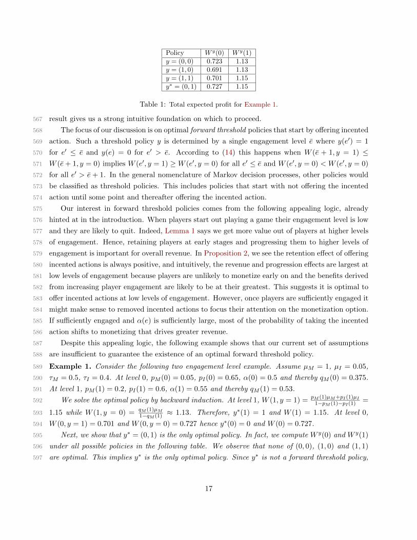
Policy W y(0) W y(1)y = (0, 0) 0.723 1.13y = (1, 0) 0.691 1.13y = (1, 1) 0.701 1.15y∗ = (0, 1) 0.727 1.15

Table 1: Total expected profit for Example 1.

result gives us a strong intuitive foundation on which to proceed.567

The focus of our discussion is on optimal forward threshold policies that start by offering incented568

action. Such a threshold policy y is determined by a single engagement level e where y(e′) = 1569

for e′ ≤ e and y(e) = 0 for e′ > e. According to (14) this happens when W (e + 1, y = 1) ≤570

W (e+ 1, y = 0) implies W (e′, y = 1) ≥W (e′, y = 0) for all e′ ≤ e and W (e′, y = 0) < W (e′, y = 0)571

for all e′ > e + 1. In the general nomenclature of Markov decision processes, other policies would572

be classified as threshold policies. This includes policies that start with not offering the incented573

action until some point and thereafter offering the incented action.574

Our interest in forward threshold policies comes from the following appealing logic, already575

hinted at in the introduction. When players start out playing a game their engagement level is low576

and they are likely to quit. Indeed, Lemma 1 says we get more value out of players at higher levels577

of engagement. Hence, retaining players at early stages and progressing them to higher levels of578

engagement is important for overall revenue. In Proposition 2, we see the retention effect of offering579

incented actions is always positive, and intuitively, the revenue and progression effects are largest at580

low levels of engagement because players are unlikely to monetize early on and the benefits derived581

from increasing player engagement are likely to be at their greatest. This suggests it is optimal to582

offer incented actions at low levels of engagement. However, once players are sufficiently engaged it583

might make sense to removed incented actions to focus their attention on the monetization option.584

If sufficiently engaged and α(e) is sufficiently large, most of the probability of taking the incented585

action shifts to monetizing that drives greater revenue.586

Despite this appealing logic, the following example shows that our current set of assumptions587

are insufficient to guarantee the existence of an optimal forward threshold policy.588

Example 1. Consider the following two engagement level example. Assume µM = 1, µI = 0.05,589

τM = 0.5, τI = 0.4. At level 0, pM (0) = 0.05, pI(0) = 0.65, α(0) = 0.5 and thereby qM (0) = 0.375.590

At level 1, pM (1) = 0.2, pI(1) = 0.6, α(1) = 0.55 and thereby qM (1) = 0.53.591

We solve the optimal policy by backward induction. At level 1, W (1, y = 1) = pM (1)µM+pI(1)µI1−pM (1)−pI(1) =592

1.15 while W (1, y = 0) = qM (1)µM1−qM (1) ≈ 1.13. Therefore, y∗(1) = 1 and W (1) = 1.15. At level 0,593

W (0, y = 1) = 0.701 and W (0, y = 0) = 0.727 hence y∗(0) = 0 and W (0) = 0.727.594

Next, we show that y∗ = (0, 1) is the only optimal policy. In fact, we compute W y(0) and W y(1)595

under all possible policies in the following table. We observe that none of (0, 0), (1, 0) and (1, 1)596

are optimal. This implies y∗ is the only optimal policy. Since y∗ is not a forward threshold policy,597

17

this implies there is no optimal forward threshold policy. /598

This example illustrates a break in the above logic. It is optimal to offer incented actions at the599

higher engagement level because of the dramatic reduction in the quitting probability when offered,600

reducing the quitting probability compared to a 0.47 quitting probability when not offering incented601

actions. Although the expected revenue per period the player stays at the highest engagement level602

is lower when incented actions are offered (0.23 as compared to 0.47), the player will stay longer and603

thus earn additional revenue. However, at the lowest engagement level, the immediate reward of not604

offering incented actions (0.462 versus 0.141) outweighs losses due to a lower chance of advancing605

to the higher engagement level.606

The goal for the remainder of this section is to devise additional assumptions that are relevant607

to the settings of interest to our paper and that guarantee the existence of an optimal forward608

threshold policy. The previous example shows how α plays a key role in determining whether a609

threshold policy is optimal or not. When incentives actions are removed the probability pI(e) is610

distributed to the monetization and quitting actions according to α(e). The associated increase611

in the probability of monetizing from pM (e) to qM (e) makes removing incented actions attractive,612

since the player is more likely to pay. However, the quitting probability increases from pQ(e) to613

qQ(e), a downside of removing incented actions. Intuitively speaking, if α(e) grows sufficiently614

quickly, the benefits will outweigh the costs of removing incented actions. From Assumption (A4.5)615

we know that α(e) increases, but this alone is insufficient. Just how quickly we require α(e) to616

grow to ensure a threshold policy requires careful analysis. This analysis results in lower bounds617

on the growth of α(e) that culminates in Theorem 1 below.618

Our first assumption on α(e) is a basic one:619

Assumption 5. α(N) = 1; that is, qQ(N) = pQ(N) and qM (N) = pM (N) + pI(N).620

It is straightforward to see that under this assumption it is never optimal to offer incented621

action at the highest engagement level. This assumption also serves as an interpretation of what it622

means to be in the highest engagement level, simply that players who are maximally engaged are no623

more likely to quit when the incented action is removed. Under this assumption, and by Bellman’s624

equation (14), every optimal policy y∗ has y∗(N) = 0. Note that this excludes the scenario in625

Example 1 and also implies that “backward” threshold policies are not optimal (except possibly626

the policy that y(e) = 0 for all e ∈ E that is both a backward and forward threshold). Given this,627

we restrict attention to forward threshold policies and drop the modifier “forward” in the rest of628

our development.629

The next step is to establish further sufficient conditions on the data that ensure that once the630

revenue, retention, and progression effects are negative, they stay negative. As in Section 4.1, we631

consider paired policies y1e and y2

e with a local change at e. Recall the notation ∆r(e|e) and ∆n(e|e)632

defined in (11) and (12), respectively. We are concerned with how ∆r(e|e) and ∆n(e|e) change with633

the starting engagement level e. It turns out that the revenue effect ∆r(e|e) always behaves in a634

18

way that is consistent with a threshold policy, without any additional assumptions.635

Proposition 4. Suppose Assumptions 1–2 hold. For every engagement level e let y1e and y2

e be636

paired policies with a local change at e. Then the revenue effect ∆r(e|e) is nonincreasing in e when637

∆r(e|e) ≥ 0. Moreover, if ∆r(e|e) < 0 for some e then ∆r(e′|e′) < 0 for all e′ ≥ e.638

This proposition says that the net revenue gain per visit to engagement level e is likely only to639

be positive (if it is ever positive) at lower engagement levels, confirming our basic intuition that640

incented actions can drive revenue from low engagement levels, but less so from highly engaged641

players. To show a similar result for the progression effect, we make the following assumption.642

Assumption 6. α(e+ 1)− α(e) > qM (e+ 1)− qM (e) for all e ∈ E.643

This provides our first general lower bound on the growth of α(e). It says that α(e) must grow644

faster than the probability qM (e) of monetizing when the incented action is not offered.645

Proposition 5. Suppose Assumptions 1–6 hold. For every engagement level e let y1e and y2

e be646

paired policies with a local change at e such that y1e and y2

e are identical to some fixed policy y (fixed647

in the sense that y is not a function of e) except at engagement level e. Then648

(a) If ∆n(e|e) < 0 for some e then ∆n(e|e′) < 0 for all e′ ≥ e.649

(b) If C(e) < 0 for some e then C(e′) < 0 for all e′ ≥ e, where C is as defined in (8).650

This result implies that once the current and future benefits of offering an incented action are651

negative, they stay negative for higher engagement levels. Indeed, Proposition 5(a) ensures that652

the future benefits F in (8) stay negative once negative, while (b) ensures the current benefits653

C stay negative once negative. In other words, once the game publisher stops offering incented654

actions it is never optimal for them to return. Note that Proposition 4 does not immediately imply655

Proposition 5(b), Assumption 6 is needed to ensure the retention effect has similar properties, as656

guaranteed by Proposition 5(a) for e′ = e.657

As mentioned above, the conditions established in Proposition 5 are necessary for the existence658

of an optimal threshold policy but does not imply that an threshold policies exists. This is because659

C and F in (8) may not switch sign from positive to negative at the same engagement level. An660

example of this is provided in Appendix A.10. We thus require one additional assumption:661

Assumption 7. 1− α(e+ 1) ≤ (1− α(e)) pM (e+1)τM+pI(e+1)τIpQ(e+1)+pM (e+1)τM+pI(e+1)τI

for e = 1, 2, . . . , N − 1.662

Note that the fractional term in the assumption is the probability of advancing from engagement663

level e+ 1 to e+ 2 conditioned on leaving engagement level e+ 1 and is thus less than one. Hence,664

this is yet another lower bound on the rate of growth in α(e), complementing Assumptions 5 and 6.665

Which bound in Assumption 6 or Assumption 7 is tighter depends on the data specifications that666

arise from specific game settings.667

Theorem 1. Suppose Assumptions 1–7 hold. Then there exists an optimal threshold policy with668

threshold engagement level e∗. That is, there exists an optimal policy y∗ with y∗(e) = 1 for any669

e ≤ e∗ and y∗(e) = 0 for any e > e∗.670

The existence of an optimal threshold is the cornerstone analytical result of this paper. From671

19

our development above, it should be clear that obtaining a sensible threshold policy is far from a672

trivial task. We believe our assumptions are reasonable based on our understanding of the games,673

given the difficult standard of guaranteeing the existence of a threshold policy. Of course, such674

policies will be welcomed in practice, precisely because of their simplicity and (relatively) intuitive675

justification. We also remark that none of these assumptions are superfluous. In Appendix A.9 we676

show that if we drop Assumption 6 then a threshold policy may longer be optimal. Appendix A.10677

shows that the same is true if Assumption 7 is dropped. As we see in some examples in the next678

section, our assumptions are sufficient but not necessary conditions for an optimal threshold policy679

to exist.680

To simplify matters further, we also take the convention that when there is a tie in Bellman’s681

equation (14) whether to offer an incented action or not, the publisher always chooses not to offer.682

This is consistent with the fact that there is a cost to offering incented actions. Although we do not683

model costs formally, we will use this reasoning to break ties. Under this tie-breaking rule there is,684

in fact, a unique optimal threshold policy guaranteed by Theorem 1. This unique threshold policy685

is our object of study in this section.686

4.3 Game design and optimal use of incented actions. So far we have provided a detailed687

analytical description of the possible benefits of offering incented actions (in Section 4.1) and688

the optimality of certain classes of policies (in Section 4.2). There remains the question of what689

types of games most benefit from offering incented actions and how different types of games may690

qualitatively differ in their optimal policies. We focus on optimal threshold policies and concern691

ourselves with how changes in the parameters of the model affect the optimal threshold e∗ of an692

optimal threshold policy y∗ that is guaranteed to exist under Assumptions 1–7 by Theorem 1. Of693

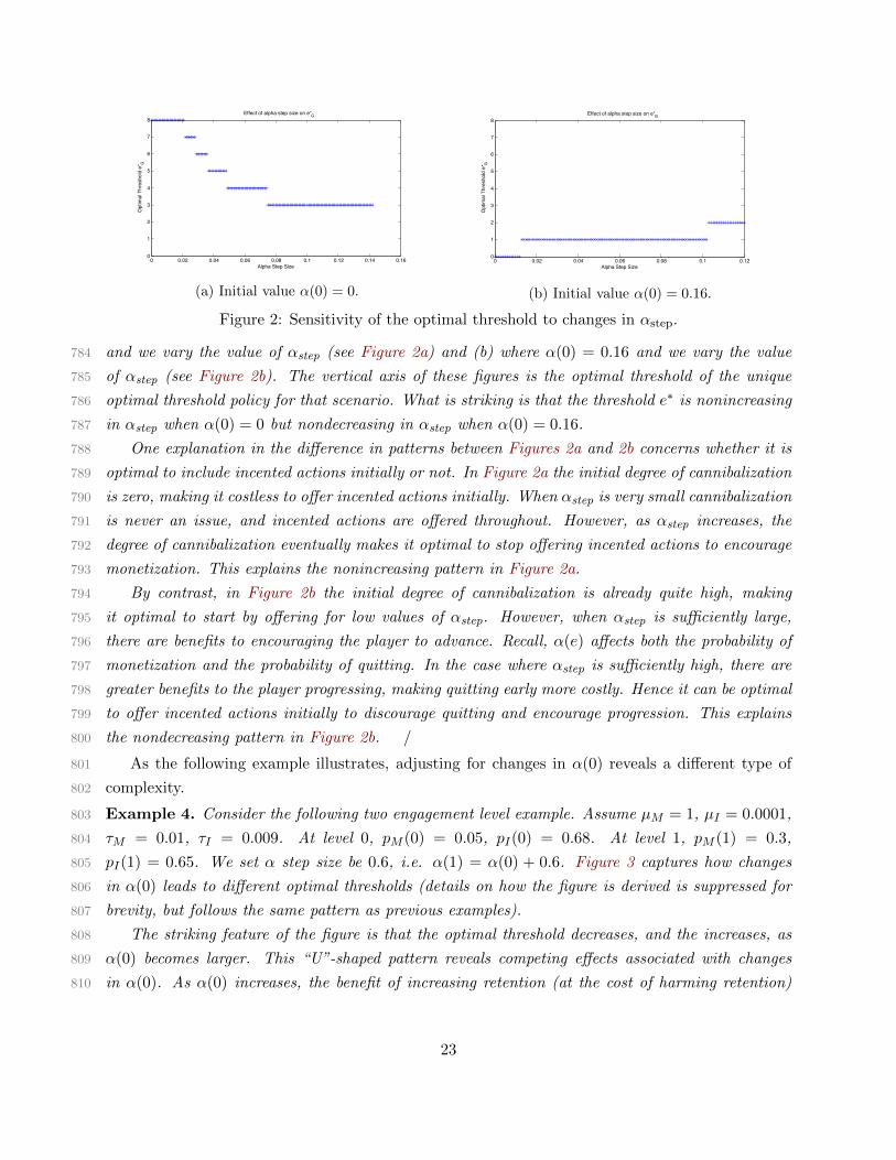
course, these are only sufficient conditions, and so we do not restrict ourselves to that setting when694

conducting numerical experiments in this section.695

We first consider how differences in the revenue parameters µI and µM affect e∗. Observe that696

only the revenue effect in (13) is impacted by changes in µI and µM , the retention and progression697

effects are unaffected. This suggests the following result:698

Proposition 6. The optimal threshold e∗ is a nondecreasing function of the ratio µIµM

.699

Note that the revenue effect is nondecreasing in the ratio µIµM

. Since the other effects are700

unchanged, this implies that the benefit of offering incented actions at each engagement level is701

nondecreasing in µIµM

, thus establishing the monotonicity of e∗ in µI/µM .702

To interpret this result, we consider what types of games have a large or small ratio µIµM

. From703

the introduction in Section 1 we know that incented actions typically deliver far less revenue to the704

publisher than in-app purchases. This suggests that the ratio is small, favoring a lower threshold.705

However, this conclusion ignores how players in the game may influence each other. Although our706

model is a single player model, one way we can include the interactions among players is through707

the revenue terms µI and µM . In many cases, a core value of a player to the game publisher is the708

20

word-of-mouth a player spreads to their contacts. Indeed, this is the value of non-paying players709

that other researchers have mostly focused on (see, for instance, Lee et al. (2017), Jiang and Sarkar710

(2009), and Gupta et al. (2009)). In cases where this “social effect” is significant, it is plausible711

that the ratio of revenue terms is not so small. For instance, if δ is the revenue attributable to the712

word-of-mouth or network effects of a player, regardless of whether the player takes an incented713

actions or monetizes, then the ratio of interest is µI+δµM+δ . The larger is δ, the larger is this ratio, and714

according to Proposition 6, the larger is the optimal threshold.715

This analysis suggests that games with a significant social component should offer incented716

actions more broadly in social games. For instance, if a game includes cooperative or competitive717

multi-player features, then spreading the player base is of particular value to the company. Thought718

of another way, in a social game it is important to have a large player base to create positive719

externalities for new players to join, and so having players quit is of greater concern in more social720

games. Hence, it is best to offer incented action until higher levels of engagement are reached. All721

of this intuition is confirmed by Proposition 6.722

Besides the social nature of the game, other factors can greatly impact of the optimal threshold.723

Genre, intended audience, and structure of the game affect the other parameters of our model;724

particularly, τI , τM , and α(e). We first examine the progression probabilities τI and τM . As we did725

in the case of the revenue parameters, we focus on the ratio τIτM

. This ratio measures the relative726

probability of advancing through incented actions versus monetization. By item (A4.4), τIτM≤ 1727

but its precise value can depend on several factors. One is the relative importance of the reward728

granted to the player when taking an incented action.729

Taking τM fixed, we note that increasing τI decreases the “current” benefit of offering incented730

actions, as seen by examining term C(e) in (8). Indeed, the revenue effect is unchanged by τI ,731

but the retention effect is weakened. The impact on future benefits is less obvious. Players are732

more likely to advance to a higher level of engagement with a larger τI . From Lemma 1 we also733

know higher engagement states are more valuable, and so we expect the future benefits of offering734

incented actions to be positive with a higher τI and even outweigh the loss in current benefits. This735

reasoning is confirmed by the next result.736

Proposition 7. The optimal threshold e∗ is a nondecreasing function of the ratio τIτM

.737

One interpretation of this result is that the more effective an incented action is at increasing738

engagement of the player, the longer the incented action should be offered. This is indeed reasonable739

under the assumption that pI(e) and pM (e) are unaffected by changes in τI . However, if increasing740

τI necessarily increases pI(e) (for instance, if the reward of the incented action becomes more741

powerful and so drives the player to take the incented action with greater probability) the effect742

on the optimal threshold is less clear.743

Example 2. In this example we show that when the incented action is more effective it can lead744

to a decrease in the optimal threshold if pI(e) and pM (e). Consider the following two engagement745

21

level example. In the base case let µM = 1, µI = 0.05, τM = 0.8, τI = 0.2. At level 0, pM (0) = 0.3,746

pI(0) = 0.5, α(0) = 0.7 and thereby qM (0) = 0.65. At level 1, pM (1) = 0.5, pI(1) = 0.4, α(1) = 1747

and thereby qM (1) = 0.9. Through basic calculations similiar to those shown in previous examples,748

one can show that the unique optimal policy is y∗ = (0, 1).749

Now change the parameters as follows: increase τI to 0.25, which affects the decision-making750

of the player so that pM (0) = 0.1, pI(0) = 0.7, pM (1) = 0.3 and pI(1) = 0.6. The incented action751

became so attractive it reduces the probability of monetizing while increasing the probability of taking752

the incented action. One can show that the unique optimal policy in this setting is y∗ = (0, 0). Hence753

the optimal threshold has decreased. In conclusion, a change in the effectiveness of the incented754

action in driving engagement can lead to an increase or decrease in the optimal threshold policy,755

depending on how the player’s behavioral response. /756

This leads to an important investigation of how changes in the degree of cannibalization between757

incented actions and monetization. Recall that α(e) is the vector of parameters that indicate the758

degree of cannibalization at each engagement level. For the sake of analysis, we assume that α(e)759

is an affine function of e with760

α(e) = α(0) + αstepe761762

where α(0) and αstep are nonnegative real numbers. A very high α(0) indicates a design where the763

reward of the incented action and the in-app purchase have a similar degree of attractiveness to the764

player so that when the incented action is removed, the player is likely to monetize. This suggests765

that the cost-to-reward ratio of the incented action is similar to that of the in-app purchase. If766

one is willing, for instance, to endure the inconvenience of watching a video ad to get some virtual767

currency, they should be similarly willing to pay real money for a proportionate amount of virtual768

currency. A very low α(0) is associated with a very attractive cost-to-reward ratio for the incented769

action that makes monetization seem expensive in comparison.770

The rate of change αstep represents the strength of an increase in cannibalization as the player771

advances in engagement. A fast rate of increase is associated with a design where the value of the772

reward of the incented action quickly diminishes. Despite the reward weakening, this option still773

attracts a lot of attention from players, especially if they have formed a habit of advancing via this774

type of reward. If, however, the videos are removed, the value proposition of monetizing seems775

attractive in comparison to the diminished value of the reward for watching a video. Seen in this776

light, the rate at which the value of the reward diminishes is controlled by the parameter αstep.777

Analysis of how different values for α(0) and αstep impact the optimal threshold is not straight-778

forward. This is illustrated in the following two examples. The first considers the sensitivity of the779

optimal threshold to αstep.780

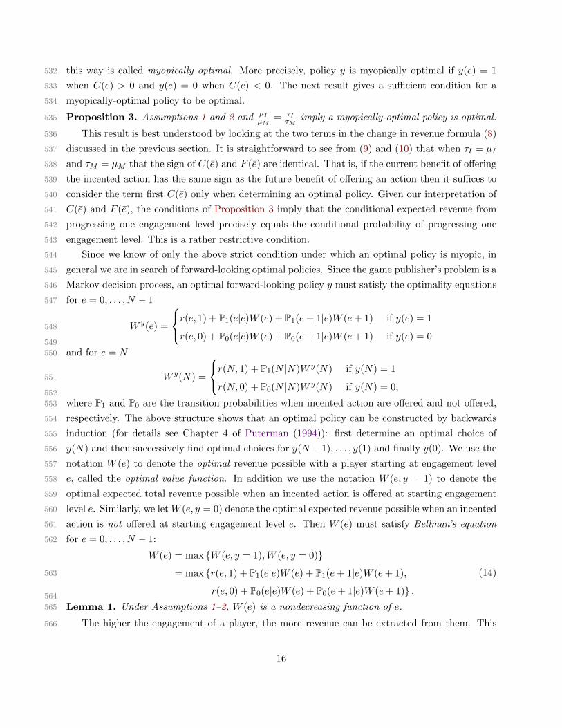
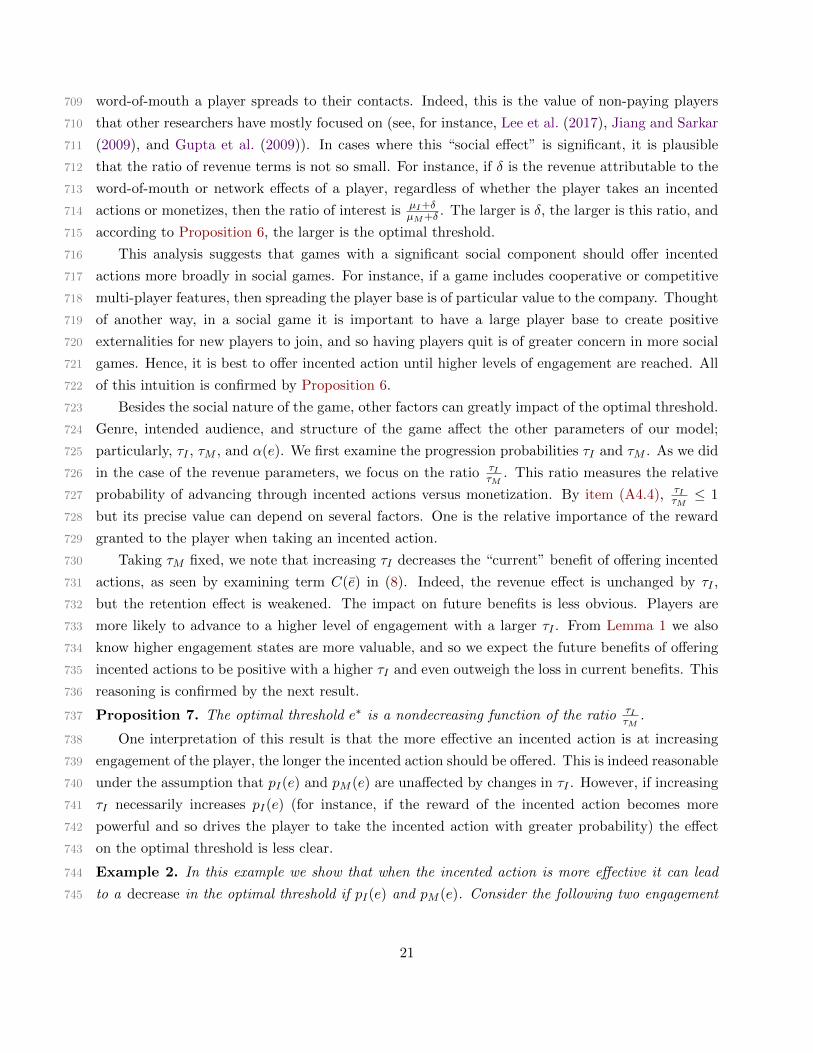
Example 3. Consider the following example with nine engagement levels and the following data:781

µm = 1, µI = 1, 0.05 τM = 0.8, τI = 0.4, pM (e) = 0.0001 + 0.00005e and pI(e) = 0.7 − 0.00001e782

for e = 0, 1, . . . , 8. We have not yet specified α(e). We examine two scenarios: (a) where α(0) = 0783

22

0 0.02 0.04 0.06 0.08 0.1 0.12 0.14 0.160

1

2

3

4

5

6

7

8

Alpha Step Size

Opt

imal

Thr

esho

ld e

* G

Effect of alpha step size on e*G

(a) Initial value α(0) = 0.

0 0.02 0.04 0.06 0.08 0.1 0.120

1

2

3

4

5

6

7

8

Alpha Step Size

Opt

imal

Thr

esho

ld e

* G

Effect of alpha step size on e*G

(b) Initial value α(0) = 0.16.

Figure 2: Sensitivity of the optimal threshold to changes in αstep.

and we vary the value of αstep (see Figure 2a) and (b) where α(0) = 0.16 and we vary the value784

of αstep (see Figure 2b). The vertical axis of these figures is the optimal threshold of the unique785

optimal threshold policy for that scenario. What is striking is that the threshold e∗ is nonincreasing786

in αstep when α(0) = 0 but nondecreasing in αstep when α(0) = 0.16.787

One explanation in the difference in patterns between Figures 2a and 2b concerns whether it is788

optimal to include incented actions initially or not. In Figure 2a the initial degree of cannibalization789

is zero, making it costless to offer incented actions initially. When αstep is very small cannibalization790

is never an issue, and incented actions are offered throughout. However, as αstep increases, the791

degree of cannibalization eventually makes it optimal to stop offering incented actions to encourage792

monetization. This explains the nonincreasing pattern in Figure 2a.793

By contrast, in Figure 2b the initial degree of cannibalization is already quite high, making794

it optimal to start by offering for low values of αstep. However, when αstep is sufficiently large,795

there are benefits to encouraging the player to advance. Recall, α(e) affects both the probability of796

monetization and the probability of quitting. In the case where αstep is sufficiently high, there are797

greater benefits to the player progressing, making quitting early more costly. Hence it can be optimal798

to offer incented actions initially to discourage quitting and encourage progression. This explains799

the nondecreasing pattern in Figure 2b. /800

As the following example illustrates, adjusting for changes in α(0) reveals a different type of801

complexity.802

Example 4. Consider the following two engagement level example. Assume µM = 1, µI = 0.0001,803

τM = 0.01, τI = 0.009. At level 0, pM (0) = 0.05, pI(0) = 0.68. At level 1, pM (1) = 0.3,804

pI(1) = 0.65. We set α step size be 0.6, i.e. α(1) = α(0) + 0.6. Figure 3 captures how changes805

in α(0) leads to different optimal thresholds (details on how the figure is derived is suppressed for806

brevity, but follows the same pattern as previous examples).807

The striking feature of the figure is that the optimal threshold decreases, and the increases, as808

α(0) becomes larger. This “U”-shaped pattern reveals competing effects associated with changes809

in α(0). As α(0) increases, the benefit of increasing retention (at the cost of harming retention)810

23

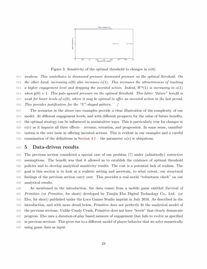
0 0.05 0.1 0.15 0.2 0.25 0.3 0.35 0.40

1

2

Alpha Initial Value: alpha(0)

Opt

imal

Thr

esho

ld e

* G

Effect of alpha(0) on e*G

Figure 3: Sensitivity of the optimal threshold to changes in α(0).

weakens. This contributes to downward pressure downward pressure on the optimal threshold. On811

the other hand, increasing α(0) also increases α(1). This increases the attractiveness of reaching812

a higher engagement level and dropping the incented action. Indeed, W y(1) is increasing in α(1)813

when y(0) = 1. This puts upward pressure on the optimal threshold. This latter “future” benefit is814

weak for lower levels of α(0), where it may be optimal to offer an incented action in the last period.815

This provides justification for the “U”-shaped pattern. /816

The scenarios in the above two examples provide a clear illustration of the complexity of our817

model. At different engagement levels, and with different prospects for the value of future benefits,818

the optimal strategy can be influenced in nonintuitive ways. This is particularly true for changes in819

α(e) as it impacts all three effects – revenue, retention, and progression. In some sense, cannibal-820

ization is the core issue in offering incented actions. This is evident in our examples and a careful821

examination of the definitions in Section 4.1 – the parameter α(e) is ubiquitous.822

5 Data-driven results823

The previous section considered a special case of our problem (7) under (admittedly) restrictive824

assumptions. The benefit was that it allowed us to establish the existence of optimal threshold825

policies and to develop analytical sensitivity results. The cost is a potential lack of realism. The826

goal is this section is to look at a realistic setting and ascertain, to what extent, our structural827

findings of the previous section carry over. This provides a real-world “robustness check” on our828

analytical results.829

As mentioned in the introduction, the data comes from a mobile game entitled Survival of830

Primitive (or Primitive, for short) developed by Tianjin Ebo Digital Technology Co., Ltd. (or831

Ebo, for short) published under the Loco Games Studio imprint in July 2016. As described in the832

introduction, and with more detail below, Primitive does not perfectly fit the analytical model of833

the previous sections. Unlike Candy Crush, Primitive does not have “levels” that clearly demarcate834

progress. Ebo uses a duration-of-play based measure of engagement that fails to evolve as specified835

in previous sections. This gives rise to a different model of player behavior that we solve numerically836

using game data as input.837

24

5.1 Data. Our data set consists of the daily game behavior of 5000 randomly selected players838

starting from the release date through 31 March 2017. For each player we have daily entries for839

play time duration, the number of incented actions taken, and the number of in-app purchases840

made. The data used to build the model has a total of 1529,577 player-day observations.841

We use this data to define engagement levels and estimate the parameters of the publisher’s842

problem in (7). We consulted with Ebo on how they defined and tracked engagement. Based on843

these conversations we tied engagement level to how “active” the player is or how “frequently”844

the player plays the game, as captured by daily gameplay durations. We computed the (moving)845

average of play durations trailing some number of days. Engagement levels then consist of discrete846

buckets of play duration averages. For our main data analysis, we chose duration buckets of 0 to 30847

minutes, 30 minutes to 60 minutes, 60 to 90 minutes and 90 to 120 minutes. That is, if the average848

time the player spent is less than 30 minutes, her engagement level is 0; between 30 minutes and849

1 hour, her engagement level is 1, etc. No player had a moving average duration greater than two850

hours, so there were four engagement levels overall.851

Another challenge is that, on a given day, there are players who neither monetize, take an852

incented action, or quit. According to our model, this day should not be considered a decision853

epoch for that player. We identified the quitting decision as follows: if the last log-in of a player854

was greater than seven days before the end of the data collection period (31 March 2017), then we855

assume that player took the quit action on the seventh data after her last log in. When we removed856

patient-day observation that did not correspond to decision epochs in our model we were left with857

123,117 observations.858

We then estimate pM , pI as follows. Given an engagement level e, let TN(e) denote the859

total number of observations where the player was in engagement level e, let MN(e) denote the860

number of these observations where a player monetized, and let IN(e) denote the number of861

these observations where a player took an incentivized action. Then our estimate of pM (e) is the862

fractionMN(e)/TN(e) and our estimate of pI(e) is the fraction IN(e)/TN(e). The quit probability863

estimate is pQ(e) = 1− pM (e)− pI(e). Table 2 captures the values we estimated from data.864

Moving average play time (min) Engagement Level (e) pI pM pQ µM µI[0, 5] 1 0.7711 0.2176 0.0113 1 0.05

(5, 30] 2 0.7552 0.2143 0.0305

(30, 60] 3 0.7576 0.2112 0.0312

(60, 90] 4 0.7621 0.2064 0.0315

(90, 120] 5 0.7534 0.2141 0.0325

Table 2: Probabilities estimated using data from Survival of Primitive.

As in Section 3, we assume that given an action a, the probability of changing engagement865

does not depend on the current engagement level (other than restricting that engagement remain866

in {0, 1, . . . , N − 1, N}). However, we relax the assumption that engagement was restricted to go867

25

up by one level. This made sense in the context of level-based engagement, not so for Primitive868

where engagement was calculated using play durations. To compute these conditional transition869

probabilities, we first calculate the total number MN =∑

eMN(e) of player-days where a mon-870

etization action occurs and the total number IN =∑

e IN(e) of player days where an incented871

action is taken. Then we calculate the total number MN+i of player-days where engagement in-872

creased by i (for i = 0, 1, . . . , N) engagement levels following a monetization action and the total873

number of MN−i of player-days where monetization was followed a decrease in engagement by874

i (for i = 1, . . . , N) engagement levels. The values IN+i and IN−i are defined analogously for875

incented actions. The resulting conditional transition probabilities, which are calculated by taking876

the appropriate ratio MN+i/MN are captured in the Table 2.877

Changes in engagement levelAction -4 -3 -2 -1 0 1 2 3 4a = M 0 0.0028 0.0123 0.1610 0.6303 0.1620 0.0203 0.0106 0.0006a = I 0 0.0032 0.0145 0.1973 0.5496 0.1984 0.0231 0.0131 0.0008

Table 3: Conditional Transition Probabilities. Rows correspond to the two action M and I. Columnscorrespond to changes in engagement level: −4 means engagement level goes down by 4 from the currentengagement level; 0 means engagement level remains the same; 4 means engagement level goes up by 4 levels,etc.

Ebo provided information on the value of a monetization action µM but did not provide infor-878

mation about µI . Typically, µI depends on a variety of factors, including the nature of the action879

(for instance the length of a video ad), and the nature of contacts with third-party providers. We880

normalize µM = 1 and set µI = 0.05 (as reflected in Table 2). This choice of µI is reasonable, the881

value of an incented action is typically cents on the dollar when compared to monetization. Other882

choices for µI were considered, with the same qualitative findings as below.883

Ideally, we would also like to provide an estimate of the cannibalization parameter α. However,884

since incented actions were always available to players during the data collection period. Thus,885

unlike estimates of µI which are available to Ebo but not part of our data set, α is not even886

currently available to Ebo. In fact, one of the proposals we made to Ebo is to experiment with887

removing incented actions for select players for a period of time to learn about α. Accordingly,888

below we will often parameterize our results regarding the parameter α. Once Ebo gets an estimate889

of α, then all the parameters of (7) can be estimated and solved numerically to optimality.890

5.2 Optimal policies. In this section, we numerically examine the structure of optimal policies891

to the publisher’s problem (7) using the parameter values estimated in Table 2. We examine how892

this optimal structure numerically depends on α, the degree of cannibalization in the game. One893

feature that stands out is the prevalence of optimal threshold contracts, where incented actions are894

offered up to a specified engagement level and thereafter removed. In a final subsection, we show895

how the threshold level depends on the parameters of the model.896

Given a value for α and the data in Table 2 we use policy iteration to determine optimal policies897

26

Figure 4: Check threshold policy when changing α(0) and αstep.

for (7). Our implementation of policy iteration is entirely standard (see for instance, Puterman898

(1994) for details). To give the reader a sense of how the optimal policies look, we take a particular899

instance of α (in fact it was chosen randomly among non-decreasing vectors), reflected in the900

second column on Table 4. The third column captures the associated optimal decision y∗ to (7)901

given this specification of α and the data in Table 2. The fourth column provides the optimal value902

W ∗(e) = W y(e) of the policy, as a function of the starting engagement level e. The optimal policy

e α(e) y∗(e) W ∗(e)1 0.0975 1 13.2242 0.2785 1 12.6563 0.5469 1 12.8154 0.9575 0 13.7925 0.9649 0 14.4

Table 4: Optimal policy and optimal value function for a specified α.903

presented in Table 4 is a threshold policy. Incented actions are offered at engagement levels at or904

below 3. For higher engagement levels incented actions are removed. This type of policy is easy to905

implement from Ebo’s perspective. Simply track the individual play of a user and have the game906

deliver ads only when average usage (as measured by a five-day moving average) is below a certain907

threshold. The technology to personalize the delivery of ads to individual players exists and is not908

uncommonly employed.909

5.2.1 Prevalence of threshold policies. The optimal threshold structure in Table 4 is not910

atypical. In fact, most instances we generated had an optimal threshold structure. We present911

some of these instances here. For visualization purposes, we focused on linear functions for α; that912

is, α(e) = α(1) + αstep(e− 1) where we systematically generated values for α(1) and αstep in [0, 1]913

independently. For each generated α we computed the optimal policy. Figure 4 captures the result:914

gray means “the optimal policy is a threshold policy”; black means “the optimal policy is not a915

threshold”; while a white color means “not applicable” because qM (e) = pM (e)+α(e)pI(e) becomes916

greater than 1 for some e which violates our assumptions. We note that no there is no “black” in917

27

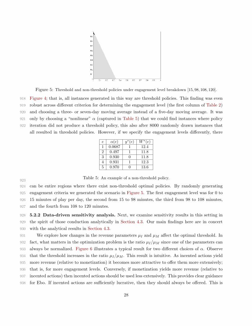
Figure 5: Threshold and non-threshold policies under engagement level breakdown [15, 98, 108, 120].

Figure 4; that is, all instances generated in this way are threshold policies. This finding was even918

robust across different criterion for determining the engagement level (the first column of Table 2)919

and choosing a three- or seven-day moving average instead of a five-day moving average. It was920

only by choosing a “nonlinear” α (captured in Table 5) that we could find instances where policy921

iteration did not produce a threshold policy, this also after 8000 randomly drawn instances that922

all resulted in threshold policies. However, if we specify the engagement levels differently, there

e α(e) y∗(e) W ∗(e)1 0.0687 1 12.42 0.497 1 11.83 0.930 0 11.84 0.931 1 12.35 0.970 0 13.6

Table 5: An example of a non-threshold policy.923

can be entire regions where there exist non-threshold optimal policies. By randomly generating924

engagement criteria we generated the scenario in Figure 5. The first engagement level was for 0 to925

15 minutes of play per day, the second from 15 to 98 minutes, the third from 98 to 108 minutes,926

and the fourth from 108 to 120 minutes.927

5.2.2 Data-driven sensitivity analysis. Next, we examine sensitivity results in this setting in928

the spirit of those conduction analytically in Section 4.3. Our main findings here are in concert929

with the analytical results in Section 4.3.930

We explore how changes in the revenue parameters µI and µM affect the optimal threshold. In931

fact, what matters in the optimization problem is the ratio µI/µM since one of the parameters can932

always be normalized. Figure 6 illustrates a typical result for two different choices of α. Observe933

that the threshold increases in the ratio µI/µM . This result is intuitive. As incented actions yield934

more revenue (relative to monetization) it becomes more attractive to offer them more extensively;935

that is, for more engagement levels. Conversely, if monetization yields more revenue (relative to936

incented actions) then incented actions should be used less extensively. This provides clear guidance937

for Ebo. If incented actions are sufficiently lucrative, then they should always be offered. This is938

28

(a) α = [0.127, 0.632, 0.815, 0.906, 0.913].(b) α = [0.805, 0.879, 0.947, 0.958, 0.965].

Figure 6: The effect of µI/µM on the optimal threshold.

the current policy of Ebo. However, Ebo’s policy to always offer incented actions is uninformed939

by knowledge of the specific value of α. This provides another justification for Ebo to at least940

attempt to learn about α if only to test how suboptimal (if at all) is their policy of always offering941

incented actions. Notice also that this conclusion supports the conclusion of the analytical result942

Proposition 6.943

We conducted similar sensitivity analysis studies as in Section 4.3 and found that our data-driven944

results confirmed the basic intuition discussed there. This illustrates a type of robustness of our945

conclusions for managing incented action in games across different defining notions of engagement.946

6 Conclusion947

In this paper, we investigated the use of incented actions in mobile games, a popular strategy for948

extracting additional revenue from players in freemium games where the vast majority of players are949

unlikely to monetize. We discussed the reasons for offering incented actions, and built an analytical950

model to assess the associated tradeoffs. This understanding leads us to define sufficient conditions951

for the optimality of threshold policies, which we later analyzed to provide managerial insights into952

what types of game designs are best suited to offering incented actions. Our approach of using953

an MDP has some direct benefit to practitioners. With player data and relevant game parameters954

that companies have access to in the age of big data, validating our model and using it to derive955

insights on the impact of certain policies is plausible.956

Our analytical approach was to devise a parsimonious stylized model that abstracts a fair deal957

from reality and yet nonetheless maintained the salient features needed to assess the impact and958

effects of offering incented actions. For instance, we assume the publisher has complete knowledge959

about the player’s transition probabilities and awareness of the engagement state. In the setting960

where transition probabilities are unknown, some statistical learning algorithm and classification961

of players into types would be required. Moreover, in the situation where engagement is difficult962

to define or measure, a partially observed Markov decision process (POMDP) model would be963

29

required, where only certain signals of the player’s underlying engagement can be observed. There964

is also the question of micro-founding the player model that we explore, asking what random utility965

model could give rise to the transition probabilities that we take as given in our model. All these966

questions are outside of our current scope but could nonetheless add realism to our approach. Of967

course, the challenge of establishing the existence of threshold policies in these extensions is likely968

to be prohibitive. Indeed, discovering analytical properties of optimal policies of any form in a969

POMDP is challenging (Krishnamurthy and Djonin, 2007). It is likely that these extensions would970

produce studies that are more algorithmic and numerical, whereas in the current study we were971

interested in deriving analytical insights.972

Finally, the current study ignores an important actor in the case of games hosted on mobile973

platforms – the platform holder. In the case of the iOS App Store, Apple has made several974

interventions that either limited or more closely monitored the practice of incented actions.8 In975

fact, the platform holder and game publisher have misaligned incentives when it comes to incented976

actions. Typically, the revenue derived from incented actions is not processed through the platform,977

whereas in-app purchases are. We feel that investigation of the incentive misalignment problem978

between platform and publisher, possibly as a dynamic contracting problem, is a promising area of979

future research. The model developed here is a building block for such a study.980

Acknowledgments981

We thank collaborators and techincal staff at Ebo Games for their able assistance. We thank several982

contacts at Tencent Games, Joost van Dreunen at SuperData, Antoine Merour at Riot Games, and983

Isaac Knowles at Scientific Revenue and Indiana University for fruitful discussions and insights into984

the video game industry as a whole.985

Notes986

9871http://appshopper.com/bestsellers/games/gros/?device=iphone9882https://play.google.com/store/apps/collection/topgrossing?hl=en9893https://www.engadget.com/2013/12/18/fun-app-store-facts-from-distimos-2013-year-in-review/9904http://www.gamesbrief.com/2011/11/conversion-rate/9915http://techcrunch.com/2016/02/23/activision-blizzard-closes-its-5-9b-acquisition-of-king-makers-of-candy-crush9926http://techcrunch.com/2013/06/12/king-quits-advertising-since-it-earns-so-much-on-candy-crush-purchases/9937https://www.gamasutra.com/blogs/MarkRobinson/20140912/225494/Why_Day_7_Retention_is_just_as_important_994

as_Day_1.php9958http://venturebeat.com/2014/06/21/apples-crackdown-on-incentivizing-app-installs-means-marketers-need-new-tricks/996

References997

A.Z. Abbasi, D.H. Ting, and H. Hlavacs. Engagement in games: Developing an instrument to998

measure consumer videogame engagement and its validation. International Journal of Computer999

Games Technology, 2017, 2017.1000

30

P. Albuquerque and Y. Nevskaya. The impact of innovation on product usage: A dynamic model1001

with progression in content consumption. Working Paper, 2012.1002

F. M. Bass. A new product growth model for consumer durables. Management Science, 15(1):1003

215–227, 1969.1004

H.K. Cheng and Y. Liu. Optimal software free trial strategy: The impact of network externalities1005

and consumer uncertainty. Information Systems Research, 23(2):488–504, 2012.1006

H.K. Cheng, S. Li, and Y. Liu. Optimal software free trial strategy: Limited version, time-locked,1007

or hybrid? Production and Operations Management, 24(3):504–517, 2015.1008

G.E. Fruchter and S.P. Sigue. Dynamic pricing for subscription services. Journal of Economic1009

Dynamics and Control, 37(11):2180–2194, 2013.1010

H. Guo, L. Hao, T. Mukhopadhyay, and D. Sun. Selling virtual currency in digital games: Impli-1011

cations on gameplay and social welfare. Working paper, 2016.1012

S. Gupta, C.F. Mela, and J.M. Vidal-Sanz. The value of a “free” customer. Working paper, 2009.1013

K. Hinderer and K.-H. Waldmann. Algorithms for countable state markov decision models with an1014

absorbing set. SIAM Journal on Control and Optimization, 43(6):2109–2131, 2005.1015

C. Jennett, A.L. Cox, P. Cairns, S. Dhoparee, A. Epps, T. Tijs, and A. Walton. Measuring1016

and defining the experience of immersion in games. International Journal of Human-Computer1017

Studies, 66(9):641–661, 2008.1018

Z. Jiang and S. Sarkar. Speed matters: The role of free software offer in software diffusion. Journal1019

of Management Information Systems, 26(3):207–240, 2009.1020

V. Krishnamurthy and D.V. Djonin. Structured threshold policies for dynamic sensor scheduling A1021

partially observed markov decision process approach. IEEE Transactions on Signal Processing,1022

55(10):4938–4957, 2007.1023

C. Lee, V. Kumar, and S. Gupta. Designing freemium: Strategic balancing growth and monetiza-1024

tion. Working paper, 2017.1025

B. Libai, E. Muller, and R. Peres. The diffusion of services. Journal of Marketing Research, 46(2):1026

163–175, 2009.1027

N. Lovell. Design Rules for Free-to-Play Games. GAMESbrief, 2012.1028

McKinsey. Global media report. http://www.mckinsey.com/client_service/media_and_1029

entertainment/latest_thinking/global_media_report_2013, 2013.1030

M.F. Niculescu and D.J. Wu. Economics of free under perpetual licensing: Implications for the1031

software industry. Information Systems Research, 25(1):173–199, 2014.1032

M.L. Puterman. Markov Decision Processes: Discrete Stochastic Dynamic Programming. Wiley,1033

1994.1034

K.T. Talluri and G.J. Van Ryzin. The Theory and Practice of Revenue Management. Springer,1035

2006.1036

H.M. Taylor and S. Karlin. An Introduction to Stochastic Modeling. Academic Press, 2014.1037

P.H. Zipkin. Foundations of Inventory Management, volume 20. McGraw-Hill New York, 2000.1038

31

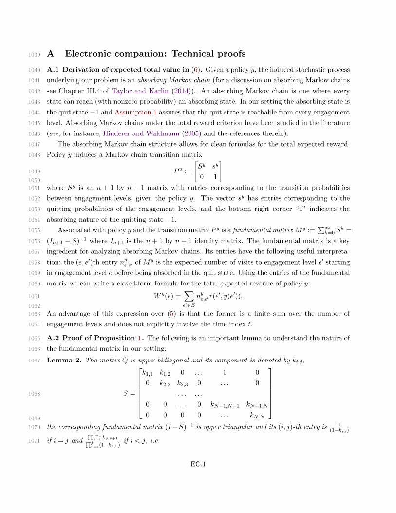
A Electronic companion: Technical proofs1039

A.1 Derivation of expected total value in (6). Given a policy y, the induced stochastic process1040

underlying our problem is an absorbing Markov chain (for a discussion on absorbing Markov chains1041

see Chapter III.4 of Taylor and Karlin (2014)). An absorbing Markov chain is one where every1042

state can reach (with nonzero probability) an absorbing state. In our setting the absorbing state is1043

the quit state −1 and Assumption 1 assures that the quit state is reachable from every engagement1044

level. Absorbing Markov chains under the total reward criterion have been studied in the literature1045

(see, for instance, Hinderer and Waldmann (2005) and the references therein).1046

The absorbing Markov chain structure allows for clean formulas for the total expected reward.1047

Policy y induces a Markov chain transition matrix1048

P y :=

[Sy sy

0 1

]1049

1050

where Sy is an n + 1 by n + 1 matrix with entries corresponding to the transition probabilities1051

between engagement levels, given the policy y. The vector sy has entries corresponding to the1052

quitting probabilities of the engagement levels, and the bottom right corner “1” indicates the1053

absorbing nature of the quitting state −1.1054

Associated with policy y and the transition matrix P y is a fundamental matrix My :=∑∞

k=0 Sk =1055

(In+1 − S)−1 where In+1 is the n + 1 by n + 1 identity matrix. The fundamental matrix is a key1056

ingredient for analyzing absorbing Markov chains. Its entries have the following useful interpreta-1057

tion: the (e, e′)th entry nye,e′ of My is the expected number of visits to engagement level e′ starting1058

in engagement level e before being absorbed in the quit state. Using the entries of the fundamental1059

matrix we can write a closed-form formula for the total expected revenue of policy y:1060

W y(e) =∑e′∈E

nye,e′r(e′, y(e′)).1061

1062

An advantage of this expression over (5) is that the former is a finite sum over the number of1063

engagement levels and does not explicitly involve the time index t.1064

A.2 Proof of Proposition 1. The following is an important lemma to understand the nature of1065

the fundamental matrix in our setting:1066

Lemma 2. The matrix Q is upper bidiagonal and its component is denoted by ki,j,1067

S =

k1,1 k1,2 0 . . . 0 0

0 k2,2 k2,3 0 . . . 0

. . . . . .

0 0 . . . 0 kN−1,N−1 kN−1,N

0 0 0 0 . . . kN,N

1068

1069

the corresponding fundamental matrix (I−S)−1 is upper triangular and its (i, j)-th entry is 1(1−ki,i)1070

if i = j and∏j−1

v=i kv,v+1∏jv=i(1−kv,v)

if i < j, i.e.1071

EC.1

(I − S)−1 =

1(1−k1,1)

k1,2

(1−k1,1)(1−k2,2) . . .∏N−2

j=1 kj,j+1∏N−1j=1 (1−kj,j)

∏N−1j=1 kj,j+1∏Nj=1(1−kj,j)

0 1(1−k2,2)

k2,3

(1−k2,2)(1−k3,3) . . .∏N−1

j=2 kj,j+1∏Nj=2(1−kj,j)

. . .

0 . . . 0 1(1−kN−1,N−1)

kN−1,N

(1−kN−1,N−1)(1−kN,N )

0 0 0 . . . 1(1−kN,N )

1072

1073

Proof. We prove the lemma by showing (I−S)× (I−S)−1 = I where (I−S)−1 is proposed above.1074

Denote R as the production of (I − S) and (I − S)−1. The (i, j)-th entry of R results from the1075

multiplication of the i-th row of (I − S) and the j-th column of (I − S)−1.1076

The i-th row of (I −S) is (0, . . . , 0, 1− ki,i︸ ︷︷ ︸i

,−ki,i+1︸ ︷︷ ︸i+1

, 0, . . . , 0). For the j-th column of (I −S)−1,1077

we consider three possible cases:1078

1) If j < i, the j-th column of (I − S)−1 is (∏j−1

v=1 kv,v+1∏jv=1(1−kv,v)

, . . . , 0︸︷︷︸i

, 0︸︷︷︸i+1

, 0, . . . , 0)T . Clearly the1079

(i, j)-th entry of R is 0.1080

2) If j = i, the j-th column of (I − S)−1 is (∏j−1

v=1 kv,v+1∏jv=1(1−kv,v)

, . . . , 1(1−ki,i)︸ ︷︷ ︸

i

, 0︸︷︷︸i+1

, 0, . . . , 0)T . So the1081

(i, i)-th entry of R is 1.1082

3) If j > i, the j-th column of (I−S)−1 is (∏j−1

v=1 kv,v+1∏jv=1(1−kv,v)

, . . . ,∏j−1

v=i kv,v+1∏jv=i(1−kv,v)︸ ︷︷ ︸

i

,∏j−1

v=i+1 kv,v+1∏jv=i+1(1−kv,v)︸ ︷︷ ︸

i+1

, 0, . . . , 0)T .1083

By simply algebra, we obtain the (i, j)-th entry of R is 0. Thus, the (i, j)-th entry of R is 1 if i = j1084

and is 0 otherwise and so R is an identity matrix.1085

In our model, ki,j indicates the transition probability from state i to state j. Suppose the1086

policy is y1, we have ke,e = qM (e)(1−τM ) and ke,e+1 = qM (e)τM . Suppose the policy is y2, we have1087

ke,e = pM (e)(1− τM ) + pI(e)(1− τI) and ke,e+1 = pM (e)τM + pI(e)τI . By definition, the expected1088

number of visits nye,e is the (e, e)-th entry of the fundamental matrix My. According to Lemma 2, we1089

have n1e,e = qM (e)τM

1−qM (e)(1−τM )×∏e−1

j=e+1 kj,j+1∏ej=e+1(1−kj,j)

and n2e,e = pM (e)τM+pI(e)τM

1−pM (e)(1−τM )−pI(e)(1−τI)×∏e−1

j=e+1 kj,j+1∏ej=e+1(1−kj,j)

. (We1090

assume∏j = e+ 1ekj,j+1 = 1). Because we only make local change of the policy at engagement1091

level e, n1e,e and n2

e,e share the same term∏e−1

j=e+1 kj,j+1∏ej=e+1(1−kj,j)

where kj,j and kj,j+1 depend on the policy1092

EC.2

y1(j) for j > e. In fact,1093

kj,j =

qM (j)(1− τM ) if y∗(j) = 0 and j < N

pM (j)(1− τM ) + pI(j)(1− τI) if y∗(j) = 1 and j < N

qM (j) if y∗(j) = 0 and j = N

pM (j) + pI(j) if y∗(j) = 1 and j = N

1094

kj,j+1 =

qM (j)τM if y∗(j) = 0 and j < N

pM (j)τM + pI(j)τI if y∗(j) = 0 and j < N1095

1096

Moreover, we find out that ny1(e+1)e+1,e =

∏e−1j=e+1 kj,j+1∏e

j=e+1(1−kj,j). Hence, we rewrite n1

e,e = qM (e)τM1−qM (e)(1−τM )n

y1(e+1)e+1,e1097

and n2e,e = pM (e)τM+pI(e)τM

1−pM (e)(1−τM )−pI(e)(1−τI)ny1(e+1)e+1,e for all e > e. Finally, the progression effect is equivalent1098

to the following:1099

∆n(e|e) = n2e,e − n1

e,e1100

= pM (e)τM+pI(e)τM1−pM (e)(1−τM )−pI(e)(1−τI)n

y1(e+1)e+1,e − qM (e)τM

1−qM (e)(1−τM )ny1(e+1)e+1,e1101

= [ pM (e)τM+pI(e)τM1−pM (e)(1−τM )−pI(e)(1−τI) −

qM (e)τM1−qM (e)(1−τM ) ]n

y1(e+1)e+1,e1102

= pI(e){τI−α(e)τM+qM (e)[(1−τI)τM−(1−τM )τI ]}[1−qM (e)(1−τM )][1−pM (e)(1−τM )−pI(e)(1−τI)]n

y1(e+1)e+1,e (15)1103

1104

Since the denominator of (15) is positive and ny1(e+1)e+1,e is positive, the sign of ∆n(e|e) is completely1105

determined by the term τI − α(e)τM + qM (e)[(1 − τI)τM − (1 − τM )τI ] for all e > e. It is only1106

affected by e but not e. It means that the progression effect is uniform in sign with respect to e.1107

A.3 Proof of Proposition 2. By definition, nye,e is the (e, e)-th entry of the fundamental matrix1108

Ny. According to Lemma 2 (in Appendix A.2) if the policy is y1, k1e,e = qM (e)(1−τM ) and thereby1109

n1e,e = 1

1−qM (e)(1−τM ) . If the policy is y2, k2e,e = pM (e)(1 − τM ) + pI(e)(1 − τI) and consequently1110

n2e,e = 1

1−pM (e)(1−τM )−pI(e)(1−τI) .1111

Therefore, the retention effect is equal to1112

∆n(e|e) = n2e,e − n1

e,e1113

= 11−pM (e)(1−τM )−pI(e)(1−τI) − 1

1−qM (e)(1−τM )1114

= [1−qM (e)(1−τM )]−[1−pM (e)(1−τM )−pI(e)(1−τI)][1−qM (e)(1−τM )][1−pM (e)(1−τM )−pI(e)(1−τI)]1115

= pI(e)[(1−τI)−α(e)(1−τM )][1−qM (e)(1−τM )][1−pM (e)(1−τM )−pI(e)(1−τI)]1116

1117

where the last equality comes from the fact qM (e) = pM (e) + α(e)pI(e). The sign of ∆n(e|e)1118

completely depends on (1 − τI) − α(e)(1 − τM ). Under Assumptions 1 to 3, we have (1 − τI) ≥1119

(1− τM ) ≥ α(e)(1− τM ). Hence the retention effect is nonnegative, i.e ∆n(e|e) ≥ 0 for all e.1120

A.4 Proof of Lemma 1. In order to prove the Theorem, we first introduce the following lemma.1121

Lemma 3. For any e = 1, . . . , N , W (e, y = 0) ≥ qM (e)µM1−qM (e) and W (e, y = 1) ≥ pM (e)µM+pI(e)µI

1−pM (e)−pI(e)1122

Proof of Lemma 3: The proof is by induction. Clearly, at the highest engagement level1123

EC.3

e = N , we have W (N, y = 0) = qM (N)µM1−qM (N) and W (N, y = 1) = pM (N)µM+pI(N)µI

1−pM (N)−pI(N) . Now suppose it1124

holds for level j ≥ e+ 1, we would like to show the result still holds for level e.1125

W (e, y = 0)− qM (e)µM1−qM (e)1126

= qM (e)µM1−qM (e)(1−τM ) + qM (e)τM

1−qM (e)(1−τM )W (e+ 1)− qM (e)µM1−qM (e)1127

= [qM (e)µM+qM (e)τMW (e+1)][1−qM (e)]−qM (e)µM [1−qM (e)(1−τM )][1−qM (e)(1−τM )][1−qM (e)]1128

= qM (e)τM [W (e+1)(1−qM (e))−qM (e)µM ][1−qM (e)(1−τM )][1−qM (e)]1129

By the inductive assumption, W (e + 1) ≥ W (e + 1, y = 0) ≥ qM (e+1)µM1−qM (e+1) ≥

qM (e)µM1−qM (e) , we finally1130

obtain W (e, y = 0)− qM (e)µM1−qM (e) ≥ 0. Similarly,1131

W (e, y = 1)− pM (e)µM+pI(e)µI1−pM (e)−pI(e)1132

= pM (e)µM+pI(e)µI1−pM (e)(1−τM )−pI(e)(1−τI) + pM (e)τM+pIτI

1−pM (e)(1−τM )−pI(e)(1−τI)W (e+ 1)− pM (e)µM+pI(e)µI1−pM (e)−pI(e)1133

= (pM (e)τM+pIτI)[W (e+1)(1−pM (e)−pI(e))−pM (e)µM−pI(e)µI ][1−pM (e)(1−τM )−pI(e)(1−τI)][1−pM (e)−pI(e)]1134

By the inductive assumption, we have W (e + 1) ≥ W (e + 1, y = 1) ≥ pM (e+1)µM+pI(e+1)µI1−pM (e+1)−pI(e+1) ≥1135

pM (e)µM+pI(e)µI1−pM (e)−pI(e) . Therefore, W (e, y = 1) − pM (e)µM+pI(e)µI

1−pM (e)−pI(e) ≥ 0. This completes the proof for1136

Lemma 3.1137

We return to the proof of Lemma 1, to show the optimal value function W (e) is increasing in1138

e. It suffices to show W (e, y = 1) ≤ W (e+ 1) and W (e, y = 0) ≤ W (e+ 1) for any e < N , in that1139

we will have W (e) = max{W (e, y = 1),W (e, y = 0)} ≤ W (e + 1). First, we compare W (e, y = 1)1140

and W (e+ 1).1141

W (e, y = 0)−W (e+ 1) = qM (e)µM1−qM (e)(1−τM ) + qM (e)τM

1−qM (e)(1−τM )W (e+ 1)−W (e+ 1)1142

= qM (e)µM1−qM (e)(1−τM ) −

1−qM (e)1−qM (e)(1−τM )W (e+ 1)1143

= 1−qM (e)1−qM (e)(1−τM ) [ qM (e)µM

1−qM (e) −W (e+ 1)] ≤ 01144

where the last equality holds because qM (e)µM1−qM (e) ≤

qM (e+1)µM1−qM (e+1) ≤ W (e + 1, y = 0) ≤ W (e + 1).1145

Similarly, we compare W (e, y = 1) and W (e+ 1).1146

W (e, y = 1)−W (e+ 1) = pM (e)µM+pI(e)µI1−pM (e)(1−τM )−pI(e)(1−τI) + pM (e)τM+pI(e)τI

1−pM (e)(1−τM )−pI(e)(1−τI)W (e+ 1)−W (e+ 1)1147

= pM (e)µM+pI(e)µI1−pM (e)(1−τM )−pI(e)(1−τI) −

1−pM (e)−pI(e)1−pM (e)(1−τM )−pI(e)(1−τI)W (e+ 1)1148

= 1−pM (e)−pI(e)1−pM (e)(1−τM )−pI(e)(1−τI) [pM (e)µM+pI(e)µI

1−pM (e)−pI(e) −W (e+ 1)] ≤ 01149

where the last equality holds since pM (e)µM+pI(e)µI1−pM (e)−pI(e) ≤ pM (e+1)µM+pI(e+1)µI

1−pM (e+1)−pI(e+1) ≤ W (e + 1, y = 1) ≤1150

W (e+ 1).1151

Finally, since W (e) = max{W (e, y = 1),W (y = 0, e)} and we have shown that both W (e, y = 1)1152

and W (e, y = 0) are no greater than W (e+ 1), we conclude that W (e) ≤W (e+ 1).1153

A.5 Proof of Proposition 3. We denote W 2(e)−W 1(e) = C(e) + F (e), where C(e) represents1154

the “current” benefits of offering incented actions and F (e) represents the “future” benefits. In1155

EC.4

order to prove the optimality of the myopic policy, we first take a close look at C(e) and F (e). By1156

definition,1157

C(e) = pM (e)µM+pI(e)µI1−pM (e)(1−τM )−pI(e)(1−τI) −

qM (e)µM1−qM (e)(1−τM )1158

= {[pM (e)µM+pI(e)µI ][1−qM (e)(1−τM )]−qM (e)µM [1−pM (e)(1−τM )−pI(e)(1−τI)]}[1−qM (e)(1−τM )][1−pM (e)(1−τM )−pI(e)(1−τI)]1159

= pI(e)[1−qM (e)(1−τM )][1−pM (e)(1−τM )−pI(e)(1−τI)]{µI − α(e)µM + qM (e)[(1− τI)µM − (1− τM )µI ]}1160

F (e) = { pM (e)τM+pI(e)τI1−pM (e)(1−τM )−pI(e)(1−τI) −

qM (e)τM1−qM (e)(1−τM )}{

∑e′>e

ny1

e+1,e′r(e′, y(e′))}1161

= {[pM (e)τM+pI(e)τI ][1−qM (e)(1−τM )]−qM (e)τM [1−pM (e)(1−τM )−pI(e)(1−τI)]}[1−qM (e)(1−τM )][1−pM (e)(1−τM )−pI(e)(1−τI)] {

∑e′>e

ny1

e+1,e′r(e′, y(e′))}1162

=pI(e){

∑e′>e n

y1(e+1)

e+1,e′ r(e′,y(e′))}

[1−qM (e)(1−τM )][1−pM (e)(1−τM )−pI(e)(1−τI)]{τI − α(e)τM + qM (e)[(1− τI)τM − (1− τM )τI ]}11631164

We further define1165

δ1(e) = µI − α(e)µM + qM (e)[(1− τI)µM − (1− τM )µI ]1166

δ2(e) = τI − α(e)τM + qM (e)[(1− τI)τM − (1− τM )τI ]11671168

Clearly, the sign of C(e) is determined by δ1(e) and the sign of F (e) is determined by δ2(e). Now1169

suppose τI/τM = µI/µM , it leads to δ1(e)/µM = δ2(e)/τM . Therefore, δ1(e) and δ2(e) must have1170

the same sign. It implies that whenever δ1(e) is positive, we must have δ2(e) positive and thereby1171

W 2(e) −W 1(e) positive. Similarly, whenever δ1(e) is negative, we must have δ2(e) negative and1172

thereby W 2(e)−W 1(e) negative.1173

Notice that the previous analysis does not rely on the policy for higher engagement level e > e.1174

Even if we fix y1(e) to be the optimal action which is solved by backward induction for e > e,1175

we still have that the “current” benefit C(e) and the “future” benefit F (e) share the same sign.1176

Therefore, the optimal action at engagement level e can be determined by whether C(e) is positive1177

or negative. Equivalently speaking, the myopically-optimal policy will be the optimal policy.1178

A.6 Proof of Proposition 4. By definition, the revenue effect is1179

∆r(e) = pM (e)µM + pI(e)µI − qM (e)µM = pI(e)[µI − α(e)µM ]11801181

where the last equality comes from the fact qM (e) = pM (e) + α(e)pI(e).1182

First of all, as pI(e) is non-negative, the sign of ∆r(e) is determined by µI − α(e)µM which is1183

decreasing in e. Thus if ∆r(e) < 0 for some e, we will also have ∆r(e′) < 0 for all e′ ≥ e.1184

Moreover, both pI(e) and µI − α(e)µM are nonincreasing in e, so we conclude that ∆r(e) is1185

nonincreasing in e whenever µI − α(e)µM > 0, i.e. whenever ∆r(e) > 0.1186

A.7 Proof of Proposition 5. (a) Recall the expression for ∆n(e|e).1187

∆n(e|e) =pI(e)n

y1(e+1)e+1,e

[1−qM (e)(1−τM )][1−pM (e)(1−τM )−pI(e)(1−τI)]{τI − α(e)τM + qM (e)[(1− τI)τM − (1− τM )τI ]}11881189

The sign of ∆n(e|e) is completely decided by δ2(e) = τI−α(e)τM +qM (e)[(1−τI)τM−(1−τM )τI ] =1190

τI − α(e)τM + qM (e)[τM − τI ].1191

EC.5

Assumption 6 indicates that −α(e)τM +qM (e)τM will decrease in e. Besides, −qM (e)τI will also1192

decrease in e. Therefore, δ2(e) will be a decreasing function of e. It implies ∆n(e|e) satisfies the1193

following property: if ∆n(e|e) > 0 for some e, then ∆n(e|e′) > 0 for all e′ ≤ e; and if ∆n(e|e) < 01194

for some e, then ∆n(e|e′) < 0 for all e′ ≥ e1195

(b) From the previous analysis, we have already seen that the sign of C(e) only depends on the1196

term δ1(e) = µI −α(e)µM + qM (e)[(1− τI)µM − (1− τM )µI ] and the sign of F (e) only depends on1197

the term δ2(e) = τI − α(e)τM + qM (e)[τM − τI ]. From (a), we have already shown that δ2(e) will1198

decrease in e. Therefore, if F (e) > 0 for some e, then F (e) > 0 for all e′ ≤ e; if F (e) < 0 for some1199

e, then F (e) < 0 for all e′ ≥ e.1200

Similarly, Assumption 6 ensures that −α(e)µM + qM (e)(1 − τI)µM will also decrease in e, in1201

that α(e + 1)µM − qM (e + 1)(1 − τI)µM − α(e)µM + qM (e)(1 − τI)µM = [α(e + 1) − α(e)]µM −1202

[qM (e + 1) − qM (e)]µM (1 − τI) ≥ µM [(α(e + 1) − α(e)) − (qM (e + 1) − qM (e))] ≥ 0. In addition,1203

−qM (e)(1− τM )µI will decrease in e as well. As a result, δ1(e) will also be an decreasing function1204

of e. Hence C(e) satisfies the following property: if C(e) > 0 for some e, then C(e) > 0 for all1205

e′ ≤ e; if C(e) < 0 for some e, then C(e) < 0 for all e′ ≥ e.1206

A.8 Proof of Theorem 1. In order to prove the optimal policy is a threshold policy, it suffices1207

to show if there exists some e such that W (e, y = 1) − W (e, y = 0) > 0, then we must have1208

W (e, y = 1)−W (e, y = 0) > 0 for all e < e.1209

First of all, Assumption 5 guarantees that it is optimal not to offer incented action at the highest1210

engagement level. Because W (N, y = 1) = pM (N)µM+pI(N)µIpQ(N) < pM (N)µM+pI(N)µM

pQ(N) = qM (N)µMqQ(N) =1211

W (N, y = 0). Suppose that W (e, y = 1)−W (e, y = 0) > 0 for some e < N where1212

W (e, y = 1)−W (e, y = 0) = pI(e)[1−qM (e)(1−τM )][1−pM (e)(1−τM )−pI(e)(1−τI)]{δ1(e) + δ2(e)

∑e>e

ny∗(e+1)e+1,e r(e, y(e))}1213

1214

so it is equivalent to assume δ1(e) + δ2(e)∑

e>e ny∗(e+1)e+1,e r(e, y(e)) > 0. It implies that at least1215

one of δ1(e) and δ2(e) has to be positive.1216

We would like to show W (e − 1, y = 1) −W (e − 1, y = 0) > 0. It suffices to show δ1(e − 1) +1217

δ2(e− 1)∑

e>e−1 ny∗(e)e,e r(e, y(e)) > 0. Now we consider three possible scenarios:1218

(1.1) Suppose δ1(e) > 0 and δ2(e) > 0. We have already proven that δ1(e) and δ2(e) are1219

decreasing functions in e under Assumption 6. Therefore, δ1(e − 1) > δ1(e) > 0 and δ2(e − 1) >1220

δ2(e) > 0. Clearly, we have W (e− 1, y = 1)−W (e− 1, y = 0) > 0 in this case.1221

(1.2) Suppose δ1(e) < 0 but δ2(e) > 0 (which may happen only if µI/µM < τI/τM ). We first1222

prove under Assumption 7, δ2(e−1)∑

e>e−1 ny∗(e)e,e r(e, y(e)) > δ2(e)

∑e>e n

y∗(e+1)e+1,e r(e, y(e)). Notice1223

that1224

δ2(e− 1)∑e>e−1

ny∗(e)e,e r(e, y(e)) = δ2(e− 1){ny

∗(e)e,e r(e, y∗(e)) + n

y∗(e)e,e+1r(e+ 1, y∗(e+ 1)) + · · ·+ n

y∗(e)e,N r(N, y∗(N))}1225

δ2(e)∑e>e

ny∗(e+1)e+1,e r(e, y(e)) = δ2(e){ny

∗(e+1)e+1,e+1r(e+ 1, y∗(e+ 1)) + · · ·+ n

y∗(e+1)e+1,N r(N, y∗(N))}1226

1227

EC.6

For e > e, we have such relationship n1e,e = pM (e)τM+pI(e)τI

1−pM (e)(1−τM )−pI(e)(1−τI)ny∗(e+1)e+1,e since y∗(e) = 1. As a1228

result,1229

δ2(e− 1)∑e>e−1

ny∗(e)e,e r(e, y(e)) = δ2(e− 1)n

y∗(e)e,e r(e, y∗(e)) + δ2(e− 1) pM (e)τM+pI(e)τI

1−pM (e)(1−τM )−pI(e)(1−τI)

∑e>e

ny∗(e+1)e+1,e r(e, y(e))1230

1231

Next we are going to show δ2(e − 1) pM (e)τM+pI(e)τI1−pM (e)(1−τM )−pI(e)(1−τI) > δ2(e) under Assumption 7. Since1232

δ2(e− 1) > δ2(e) > 0, we can compare δ2(e)δ2(e−1) with pM (e)τM+pI(e)τI

1−pM (e)(1−τM )−pI(e)(1−τI) . For the ratio δ2(e)δ2(e−1) ,1233

we have1234

δ2(e)δ2(e−1) = τI−α(e)τM+qM (e)[τM−τI ]

τI−α(e−1)τM+qM (e−1)[τM−τI ] = τI/τM−α(e)+qM (e)[1−τI/τM ]τI/τM−α(e−1)+qM (e−1)[1−τIτM ]1235

= 1−qM (e)1−qM (e−1) +

[α(e−1)−qM (e−1)]1−qM (e)

1−qM (e−1)−[α(e)−qM (e)]

τI/τM−α(e−1)+qM (e−1)[1−τI/τM ] ≤ 1−α(e)1−α(e−1) (16)1236

1237

Because [α(e − 1) − qM (e − 1)] 1−qM (e)1−qM (e−1) − [α(e) − qM (e)] < 0 and 1 − qM (e − 1) > 0, the ratio1238

δ2(e)δ2(e−1) will increase in τI/τM and reach maximum when τI/τM = 1. We achieve (16).1239

Finally, Assumption 7 claims that 1−α(e)1−α(e−1) ≤

pM (e)τM+pI(e)τI1−pM (e)(1−τM )−pI(e)(1−τI) . Hence, we end up with1240

δ2(e− 1) pM (e)τM+pI(e)τI1−pM (e)(1−τM )−pI(e)(1−τI) > δ2(e). We further have1241

δ2(e− 1)∑e>e−1

ny∗(e)e,e r(e, y(e)) = δ2(e− 1)n2

e,er(e, y∗(e))1242

+ δ2(e− 1) pM (e)τM+pI(e)τI1−pM (e)(1−τM )−pI(e)(1−τI)

∑e>e

ny∗(e+1)e+1,e r(e, y(e))1243

> δ2(e)∑e>e

ny∗(e+1)e+1,e r(e, y(e))1244

1245

Finally we conclude1246

δ1(e− 1) + δ2(e− 1)∑e>e−1

ny∗(e)e,e r(e, y(e)) > δ1(e) + δ2(e)

∑e>e

ny∗(e+1)e+1,e r(e, y(e)) > 01247

1248

equivalently, we have W (e− 1, y = 1)−W (e− 1, y = 0) > 0 in this case.1249

(1.3) Suppose δ1(e) > 0 but δ2(e) < 0 (which may happen only if µI/µM > τI/τM ). If1250

δ2(e − 1) ≥ 0, we easily get δ1(e − 1) + δ2(e − 1)W (e) > δ1(e) + δ2(e − 1)W (e) > 0. Else if1251

0 > δ2(e − 1) ≥ δ2(e), Lemma 1 indicates that 0 ≤ W (e) ≤ W (e + 1), therefore we have δ2(e −1252

1)W (e) > δ2(e)W (e) > δ2(e)W (e + 1). Finally, δ1(e − 1) + δ2(e − 1)∑

e>e−1 ny∗(e)e,e r(e, y(e)) =1253

δ1(e − 1) + δ2(e − 1)W (e) > δ1(e) + δ2(e)W (e + 1) = δ1(e) + δ2(e)∑

e>e ny∗(e+1)e+1,e r(e, y(e)) > 0.1254

Therefore, W (e− 1, y = 1)−W (e− 1, y = 0) > 0.1255

In conclusion, we have shown that once W (e, y = 1)−W (e, y = 0) > 0 for some e, we must also1256

have W (e − 1, y = 1) −W (e − 1, y = 0) > 0. As a result, the optimal policy should be a forward1257

threshold policy.1258

A.9 Example of a non-threshold policy where Assumption 6 is violated. Consider the1259

following two engagement level example. Assume µM = 1, µI = 0.27, τM = 0.99, τI = 0.25. At level1260

0, pM (0) = 0.23, pI(0) = 0.54, α(0) = 0.75 and thereby qM (0) = 0.635. At level 1, pM (1) = 0.34,1261

pI(1) = 0.52, α(1) = 0.81 and thereby qM (1) = 0.7612. At level 2, pM (2) = 0.42, pI(2) = 0.45,1262

EC.7

α(2) = 1 and thereby qM (1) = 0.87.1263

The optimal policy is y∗ = (0, 1, 0). We use backward induction. At the highest level 2, we1264

have y∗(2) = 0 and W (2) = 6.692. At level 1, W (1, y = 1) = 5.9395 and W (1, y = 0) = 5.849,1265

therefore y∗(1) = 1 and W (1) = W (1, y = 1) = 5.9395. Finally, at level 0, W (0, y = 1) = 4.26841266

and W (0, y = 0) = 4.3969 and so y∗(0) = 0 and W (0) = W (0, y = 0) = 4.3969. The optimal policy1267

is not a threshold policy.1268

In fact, Assumption 6 is violated because α(1) − α(0) = 0.06 while qM (1) − qM (0) = 0.1262.1269

Assumption 7 is satisfied since 1− α(1) = 0.19 and (1− α(0)) pM (1)τM+pI(1)τI(1−pM (1)(1−τM )−pI(1)(1−τI)) = 0.1923.1270

A.10 Example of non-threshold policy where Assumption 7 is violated. Consider the1271

following two engagement level example. Assume µM = 1, µI = 0.2, τM = 0.91, τI = 0.47. At level1272

0, pM (0) = 0.03, pI(0) = 0.51, α(0) = 0.59 and thereby qM (0) = 0.3309. At level 1, pM (1) = 0.05,1273

pI(1) = 0.5, α(1) = 0.62 and thereby qM (1) = 0.36. At level 2, pM (2) = 0.34, pI(2) = 0.45,1274

α(2) = 1 and thereby qM (1) = 0.79.1275

The optimal policy is y∗ = (0, 1, 0). We use backward induction to show this. At the highest1276

level 2, we have y∗(2) = 0 and W (2) = 3.7619. At level 1, W (1, y = 1) = 1.6498 and W (1, y =1277

0) = 1.6459, therefore y∗(1) = 1 and W (1) = W (1, y = 1) = 1.6498. Moreover, C(1) = −0.16681278

and F (1) = 0.1708. Finally, we look at level 0. Note that W (0, y = 1) = 0.7876 and W (0, y =1279

0) = 0.8532, as we can see y∗(0) = 0 and W (0) = W (0, y = 0) = 0.8532. Besides, C(0) = −0.15951280

and F (0) = 0.0939. The optimal policy is not a threshold policy. In fact, Assumption 6 is satisfied1281

since α(1)− α(0) = 0.03 while qM (1)− qM (0) = 0.0291.1282

A.11 Proof of Proposition 6. We will restrict ourselves only to threshold policies. According1283

to the backward induction, in order to prove the optimal threshold is non-decreasing in µI , we only1284

need to show W 2(e) −W 1(e) is non-decreasing in µI given that y1(e′) = 0 for e′ > e. Because1285

the optimal threshold e∗ is solved by W 2(e∗) − W 1(e∗) > 0 where y1(e′) = 0 for e′ > e∗ and1286

W 2(e∗ + 1)−W 1(e∗ + 1) ≤ 0 where y1(e′) = 0 for e′ > e∗ + 1.1287

We have already characterized the explicit expression for W 2(e)−W 1(e) which is1288

W 2(e)−W 1(e) =

pI(e)

[1−qM (e)(1−τM )][1−pM (e)(1−τM )−pI(e)(1−τI)]{δ1(e) + δ2(e)∑

e′>e ny1(e+1)e+1,e′ r(e

′, y(e′))} if e < N

pI(N)pQ(N)qQ(N){µI − α(N)µM + qM (N)(µM − µI)} if e = N

1289

where δ1(e) = [µI − α(e)µM + qM (e)(1− τI)µM − qM (e)(1− τM )µI ]1290

δ2(e) = [τI − α(e)τM + qM (e)(τM − τI)]12911292

Clearly, W 2(N) − W 1(N) will increase in µI . For any e < N , δ1(e) will increase in µI while1293

δ2(e) will keep constant. In addition, both ny1(e+1)e+1,e′ and r(e′, y(e′)) will remain the same since we1294

fix y1(e′) = 0 unchanged for all e′ > e. Hence, W 2(e) − W 1(e) will increase in µI . Let e∗ be1295

the largest engagement level such that W 2(e) −W 1(e) > 0. By definition, e∗ is actually the new1296

optimal threshold under a larger µI . Since originally W 2(e∗) − W 1(e∗) > 0 and the difference1297

W 2(e) − W 1(e) is increasing in µI , we conclude that e∗ ≥ e∗. The optimal threshold must be1298

EC.8

non-decreasing in µI .1299

A.12 Proof of Proposition 7. Similar to Proposition 6, we will still restrict ourselves to threshold1300

policies. It suffices to show W 2(e)−W 1(e) is non-decreasing in τI given that y1(e′) = 0 for e′ > e.1301

Obviously, W 2(N) − W 1(N) does not depend on τI . For e < N , since y1(e′) = 0 for e′ >1302

e, we have r(e′, y(e′)) and ny1(e+1)e+1,e′ unrelated with τI . Therefore, W 1(e) = qM (e)µM

1−qM (e)(1−τM ) +1303

qM (e)τM1−qM (e)(1−τM )

∑e′>e n

y1(e+1)e+1,e′ r(e

′, y(e′)) will not be affected by τI . Now we would like to show1304

W 2(e) = pM (e)µM+pI(e)µI1−pM (e)(1−τM )−pI(e)(1−τI) + pM (e)τM+pI(e)τI

1−pM (e)(1−τM )−pI(e)(1−τI)

∑e′>e n

y1(e+1)e+1,e′ r(e

′, y(e′)) will increase1305

in τI . In fact, if τI increases by ε > 0, we have1306

[ pM (e)µM+pI(e)µI1−pM (e)(1−τM )−pI(e)(1−τI−ε) + pM (e)τM+pI(e)(τI+ε)

1−pM (e)(1−τM )−pI(e)(1−τI−ε)

∑e′>e

ny1(e+1)e+1,e′ r(e

′, y(e′))]1307

− [ pM (e)µM+pI(e)µI1−pM (e)(1−τM )−pI(e)(1−τI) + pM (e)τM+pI(e)τI

1−pM (e)(1−τM )−pI(e)(1−τI)

∑e′>e

ny1(e+1)e+1,e′ r(e

′, y(e′))]1308

=εpI(e)qQ(e)

[1−pM (e)(1−τM )−pI(e)(1−τI−ε)][1−pM (e)(1−τM )−pI(e)(1−τI)]{∑e′>e

ny1(e+1)e+1,e′ r(e

′, y(e′))− pM (e)µM+pI(e)µIpQ(e) }1309

=εpI(e)qQ(e)

[1−pM (e)(1−τM )−pI(e)(1−τI−ε)][1−pM (e)(1−τM )−pI(e)(1−τI)]{W y1(e+ 1)− pM (e)µM+pI(e)µI

pQ(e) } > 0 (17)13101311

where W y1(e+ 1) is the revenue at engagement level e+ 1 if Publisher follows the policy y1(e′) = 01312

for all e′ > e. The inequality (17) holds because of Lemma 3. As a result, W 2(e) will increase in1313

τI and consequently W 2(e)−W 1(e) will increase in τI for all e < N . This implies that the optimal1314

threshold must be non-decreasing in τI .1315

EC.9