Incentives and Stability in

Large Two-Sided Matching Markets ∗

Fuhito Kojima† Parag A. Pathak‡

January 2009

Abstract

A number of labor markets and student placement systems can be modeled asmany-to-one matching markets. We analyze the scope for manipulation in many-to-onematching markets under the student-optimal stable mechanism when the number ofparticipants is large. Under some regularity conditions, we show that the fraction ofparticipants with incentives to misrepresent their preferences when others are truthfulapproaches zero as the market becomes large. With an additional condition, truthfulreporting by every participant is an approximate equilibrium under the student-optimalstable mechanism in large markets.

Keywords: Large markets, stability, two-sided matching.JEL Class: C78, D61, D78.

∗We appreciate helpful discussions with Attila Ambrus, Eric Budish, Federico Echenique, Drew Fuden-berg, Akihiko Matsui, Alvin E. Roth, Tayfun Sonmez, Satoru Takahashi and seminar participants at Harvard,Hitotsubashi, Kyoto, Osaka, Tokyo, 2006 North American Summer Meetings of the Econometric Society atMinneapolis, the 17th International Conference on Game Theory at SUNY Stony Brook and 2006 INFORMSAnnual Meeting at Pittsburgh. Discussions with Michihiro Kandori and Yohei Sekiguchi were especially impor-tant for the current version of the paper. Detailed comments by the co-editor and anonymous referees greatlyimproved the substance and exposition of the paper. For financial support, Pathak is grateful to the NationalScience Foundation, the Spencer Foundation, and the Division of Research at Harvard Business School.

†Cowles Foundation, Yale University, New Haven, CT 06510, e-mail: fuhitokojima1979@gmail.com.‡Society of Fellows, Harvard University, Cambridge, MA 02138 and Department of Economics, Massachusetts

Institute of Technology, Cambridge, MA 02142, e-mail: ppathak@fas.harvard.edu.

1

In recent years, game theoretic ideas have been used to study the design of markets. Auctionshave been employed to allocate radio spectrum, timber, electricity, and natural gas involvinghundreds of billions of dollars worldwide (Paul R. Milgrom 2004). Matching procedures havefound practical applications in centralized labor markets as well as school assignment systems inNew York City and Boston.1 Connections between auctions and matching have been exploredand extended (Alexander Kelso and Vincent Crawford 1982, John Hatfield and Milgrom 2005,and Robert Day and Milgrom 2007).

The practical aspects of market design have led to an enrichment of the theory of marketdesign. This paper investigates a theoretical problem motivated by the use of stable match-ing mechanisms in large markets, inspired by a practical issue first investigated by Roth andPeranson (1999).2 A matching is stable if there is no individual agent who prefers to becomeunmatched or pair of agents who prefer to be assigned to each other to being assigned theirallocation in the matching. In real-world applications, empirical studies have shown that stablemechanisms often succeed whereas unstable ones often fail.3

Although stable mechanisms have a number of virtues, they are susceptible to varioustypes of strategic behavior before and during the match. Roth (1982) shows that any stablemechanism is manipulable via preference lists: for some participants, reporting a true preferencelist (ordinal ranking over potential matches) may not be a best response to reported preferencesof others. In many-to-one markets such as matching markets between colleges and students,where some colleges have more than one position, Sonmez (1997) and Sonmez (1999) showthat there are additional strategic concerns. First, any stable mechanism is manipulable viacapacities, that is, colleges may sometimes benefit by underreporting their quotas. Second, anystable mechanism is manipulable via pre-arranged matches; that is, a college and a student maybenefit by agreeing to match before receiving their allocations from the centralized matchingmechanism.

Concerns about the potential for these types of manipulation are often present in realmarkets. For instance, in New York City (NYC) where the Department of Education hasrecently adopted a stable mechanism, the Deputy Chancellor of Schools described principalsconcealing capacity as a major issue with their previous unstable mechanism (New York Times11/19/04):

“Before you might have a situation where a school was going to take 100 new

1For a survey of this theory, see Alvin E. Roth and Marilda Sotomayor (1990). For applications to labormarkets, see Roth (1984a) and Roth and Elliot Peranson (1999). For applications to student assignment, see forexample Atila Abdulkadiroglu and Tayfun Sonmez (2003), Abdulkadiroglu, Pathak, Roth and Sonmez (2005),and Abdulkadiroglu, Pathak, and Roth (2005).

2A recent paper by Jeremy Bulow and Jon Levin (2006) theoretically investigates a matching market withprice competition, motivated by an antitrust case against the National Residency Matching Program. See alsoMuriel Niederle (2007).

3For a summary of this evidence, see Roth (2002).

2

children for 9th grade, they might have declared only 40 seats, and then placed theother 60 outside of the process.”4

Roth and Uriel G. Rothblum (1999) discuss similar anecdotes about preference manipulationfrom the National Resident Matching Program (NRMP), which is an entry-level matchingmarket for hospitals and medical school graduates in the U.S.

The aim of this paper is to understand why despite these negative results many stablemechanisms appear to work well in practice. We focus on the student-optimal stable mechanism,which forms the basis of many matching mechanisms used in the field such as in NYC and theNRMP. Lester E. Dubins and David A. Freedman (1981) and Roth (1982) show that studentsdo not have incentives to manipulate markets with the student-optimal stable mechanism,though colleges do have incentives to do so. Our results show that the mechanism is immuneto various kinds of manipulations by colleges when the market is large. In real-world two-sided matching markets, there are often a large number of applicants and institutions, and eachapplicant submits a preference list containing only a small fraction of institutions in the market.For instance, in the NRMP, the length of the applicant preference list is about 15, while thenumber of hospital programs is between 3,000 and 4,000 and the number of students is over20,000 per year. In NYC, about 75% of students submit preference lists of less than 12 schools,and there are about 500 school programs and over 90,000 students per year.5 Motivated bythese features, we study how the scope for manipulations changes when the number of marketparticipants grows but the length of the preference lists does not.

We consider many-to-one matching markets with the student-optimal stable mechanism,where colleges have arbitrary preferences such that every student is acceptable, and studentshave random preferences of fixed length drawn iteratively from an arbitrary distribution. Weshow that the expected proportion of colleges that have incentives to manipulate the student-optimal stable mechanism when every other college is truth-telling converges to zero as thenumber of colleges approaches infinity. The key step of the proof involves showing that, whenthere are a large number of colleges, the chain reaction caused by a college’s strategic rejectionof a student is unlikely to make another more preferred student apply to that college.6

4A careful reader may recognize that this quote is not about a stable mechanism but about an unstableone. We present this quote just to suggest that strategic behavior may be a realistic problem in general.Indeed, concern about strategic behavior motivated New York City’s recent adoption of a stable mechanism,and this paper suggests that scope for manipulations may be limited under the current stable mechanism despitetheoretical possibility of manipulation.

5For data regarding the NRMP, see http://www.nrmp.org/2006advdata.pdf. For data regarding New YorkCity high school match, see Abdulkadiroglu, Pathak and Roth (2008).

6Throughout the paper we focus on the SOSM. The college-optimal stable mechanism can be similarlydefined by letting colleges propose to students. By making complementary assumptions about the model, wecan derive results concerning incentives of students under the college-optimal stable mechanism similar to thosein the current paper. However, additional assumptions may be needed for analyzing the incentives of collegesin this case, since truth-telling is not a dominant strategy for colleges with a quota larger than one in the

3

The above result does not necessarily mean that agents report true preferences in equi-librium. Thus we also conduct equilibrium analysis in the large market. We introduce anadditional condition, called sufficient thickness, and show that truthful reporting is an approx-imate equilibrium in a large market that is sufficiently thick.

Related literature

Our paper is most closely related to Roth and Peranson (1999) and Nicole Immorlica andMohammed Mahdian (2005). Roth and Peranson (1999) conduct a series of simulations ondata from the NRMP and on randomly generated data. In their simulations, very few agentscould have benefited by submitting false preference lists or by manipulating capacity in largemarkets when every other agent is truthful. These simulations lead them to conjecture thatthe fraction of participants with preference lists of limited length who can manipulate tends tozero as the size of the market grows.7

Immorlica and Mahdian (2005), which this paper builds upon, theoretically investigate one-to-one matching markets where each college has only one position and show that as the sizeof the market becomes large, the proportion of colleges that are matched to the same studentin all stable matchings approaches one. Since a college does not have incentives to manipulatevia preference lists if and only if it is matched to the same student in all stable matchings (seeDavid Gale and Sotomayor 1985 and Gabrielle Demange, Gale and Sotomayor 1987), this resultimplies that most colleges cannot manipulate via preference lists when the market is large.

While this paper is motivated by these previous studies, there are a number of crucialdifferences. First, our focus in this paper is on many-to-one markets, which include severalreal-world markets such as the NRMP and the school choice program in NYC. In such marketsa college can sometimes manipulate via preference lists even if the college is matched to thesame set of students in all stable matchings.8 Moreover, in many-to-one markets there existsthe additional possibilities of capacity manipulation and manipulation via pre-arrangement(unraveling) which are not present in a one-to-one market.9 We introduce new techniques toovercome these complications.

Second, previous research mostly focuses on counting the average number of participantsthat can manipulate the student-optimal stable mechanism, assuming that others report their

college-optimal stable mechanism.7The property that in large matching problems the size of the set of stable matchings has also been docu-

mented using data from Boston Public School’s assignment system. Pathak and Sonmez (2007) report that inBoston, for the first two years of data from SOSM, in elementary school, the student-optimal stable matchingand college-optimal stable matching coincide, while for middle school, at most three students are assigned todifferent schools in the two matchings.

8For instance, see the example in Theorem 5.10 of Roth and Sotomayor (1990).9Indeed, Roth and Peranson (1999) explicitly investigate the potential for capacity manipulation in their

simulations.

4

preferences truthfully. This leaves open the question of whether participants will behave truth-fully in equilibrium. A substantial part of this paper investigates this question and shows thattruthful reporting is an approximate equilibrium in a large market that is sufficiently thick.10

Incentive properties in large markets are studied in other areas of economics. For example, inthe context of double auctions, Thomas Gresik and Mark Satterthwaite (1989), Aldo Rustichini,Sattherwaite, and Steven Williams (1994), Wolfgang Pesendorfer and Jeroen Swinkels (2000),Swinkels (2001), Drew Fudenberg, Markus Mobius, and Adam Szeidl (2005), and Martin Crippsand Swinkels (2006) show that the equilibrium behavior converges to truth-telling as the numberof traders increases under various informational structures. Papers more closely related to oursare discussed in Section 4.

There is a literature that analyzes the consequences of manipulations via preference listsand capacities in complete information finite matching markets. See Roth (1984b), Roth (1985)and Sonmez (1997b) for games involving preference manipulation and Hideo Konishi and UtkuUnver (2005) and Kojima (2006) for games of capacity manipulation. Some of the papers mostrelevant to ours are discussed in Section 4.

The paper proceeds as follows. Section 1 presents the model and introduces a lemma whichis key to our analysis. Section 2 defines a large market and presents our main result. Section3 conducts equilibrium analysis. Section 4 concludes. All proofs are in the Appendix.

1 Model

1.1 Preliminary definitions

Let there be a set of students S and a set of colleges C. Each student s has a strict preferencerelation Ps over the set of colleges and being unmatched (being unmatched is denoted by s).Each college c has a strict preference relation ≻c over the set of subsets of students. If s ≻c ∅,then s is said to be acceptable to c. Similarly, c is acceptable to s if cPss. A market is tupleΓ = (S, C, PS,≻C) where PS = (Ps)s∈S,≻C= (≻c)c∈C .

Since only rankings of acceptable mates matter for our analysis, we often write only accept-able mates to denote preferences. For example,

Ps : c1, c2,

means that student s prefers college c1 most, then c2, and c1 and c2 are the only acceptablecolleges.

For each college c ∈ C and any positive integer qc, its preference relation ≻c is responsivewith quota qc if the ranking of a student is independent of her colleagues, and any set of

10Immorlica and Mahdian (2005) claim that truth-telling is an approximate equilibrium in a one-to-one marketeven without sufficient thickness. In section 4, we present an example to show that this is not the case, buttruth-telling is an approximate equilibrium under an additional assumption of sufficient thickness.

5

students exceeding quota qc is unacceptable (see Roth (1985) for a formal definition).11 We willassume that all preferences are responsive throughout the paper.

Let Pc be the corresponding preference list of college c, which is the preference relationover individual students and ∅. Sometimes only the preference list structure and quotas arerelevant for the analysis. We therefore sometimes abuse notation and denote by Γ = (S, C, P, q)an arbitrary market in which the preferences induce preference lists P = (Pi)i∈S∪C and quotasq = (qc)c∈C. We say that (S, C, PS,≻C) induces (S, C, P, q) in such a case. We also use thefollowing notation: P−i = (Pj)j∈S∪C\i and q−c = (qc′)c′∈C\c.

A matching µ is a mapping from C ∪ S to itself such that (i) for every s, |µ(s)| = 1, andµ(s) = s if µ(s) /∈ C, (ii) µ(c) ⊆ S for every c ∈ C, and (iii) µ(s) = c if and only if s ∈ µ(c).That is, a matching simply specifies the college where each student is assigned or if the studentis unmatched, and the set of students assigned to each college if any.

We say a matching µ is blocked by a pair of student s and college c if s strictly prefers cto µ(s) and either (i) c strictly prefers s to some s′ ∈ µ(c) or (ii) |µ(c)| < qc and s is acceptableto c. In words, the student s in the pair prefers college c over her assignment in µ, and collegec prefers s either because it has a vacant seats or s is more preferred than another studentassigned to c under µ. A matching µ is individually rational if for each student s ∈ S,µ(s)Ps∅ or µ(s) = ∅ and for each c ∈ C, (i) |µ(c)| ≤ qc and (ii) s ≻c ∅ for every s ∈ µ(c).A matching µ is stable if it is individually rational and is not blocked. A mechanism is asystematic way of assigning students to colleges. A stable mechanism is a mechanism thatyields a stable matching with respect to reported preferences for every market.

We consider the student-optimal stable mechanism (SOSM), denoted by φ, which isanalyzed by Gale and Lloyd Shapley (1962).12

• Step 1: Each student applies to her first choice college. Each college rejects the lowest-ranking students in excess of its capacity and all unacceptable students among those whoapplied to it, keeping the rest of the students temporarily (so students not rejected atthis step may be rejected in later steps).

In general,

• Step t: Each student who was rejected in Step (t-1) applies to her next highest choice(if any). Each college considers these students and students who are temporarily heldfrom the previous step together, and rejects the lowest-ranking students in excess of itscapacity and all unacceptable students, keeping the rest of the students temporarily (sostudents not rejected at this step may be rejected in later steps).

11Note that given a responsive preference with quota ≻c, we can always find a utility function uc : S → R withthe property that for all S′, S′′ ⊆ S such that |S′|, |S′′| ≤ qc, S

′ ≻c S′′ if and only if∑

s∈S′ uc(s) >∑

s∈S′′ uc(s).We will use a particular additive representation of responsive preferences in Section 3.

12The SOSM is known to produce a stable matching that is unanimously most preferred by every studentamong all stable matchings (Gale and Shapley 1962).

6

The algorithm terminates either when every student is matched to a college or every un-matched student has been rejected by every acceptable college. The algorithm always termi-nates in a finite number of steps. Gale and Shapley (1962) show that the resulting matchingis stable. For two preference relations that induce the same pair of preference lists and quotas,the outcome of the algorithm is the same. Thus we sometimes write the resulting matching byφ(S, C, P, q). We denote by φ(S, C, P, q)(i) the assignment given to i ∈ S ∪ C under matchingφ(S, C, P, q).

1.2 Manipulating the student-optimal stable mechanism

We illustrate two ways that the SOSM can be manipulated through a simple example.

Example 1. Consider the following market with two colleges c1 and c2, and five studentss1, ..., s5. Suppose qc1 = 3 and qc2 = 1, and the preference lists of colleges are

Pc1 : s1, s2, s3, s4, s5,

Pc2 : s3, s2, s1, s4, s5,

and student preferences are

Ps1 : c2, c1,

Ps2 : c1, c2,

Ps3 : c1, c2,

Ps4 : c1, c2,

Ps5 : c1, c2.

The matching produced by the SOSM is

µ =

(

s2 s3 s4 s1

c1 c1 c1 c2

)

,

which means that c1 is matched to s2, s3 and s4, c2 is matched to s1 and s5 is unmatched.13

The first type of manipulation we will focus on is a preference manipulation (manipu-lation via preference lists), first identified by Dubins and Freedman (1981). Suppose collegec1 submitted the following preference list:

P ′c1

: s1, s2, s5, s4, s3,

13Similar notation is used throughout the paper.

7

while reporting its true quota, 3. Then the SOSM produces the following matching:

µ′ =

(

s1 s2 s5 s3

c1 c1 c1 c2

)

.

If c1 prefers {s1, s2, s5} to {s2, s3, s4}, say because student s1 is particularly desirable, thenit can benefit by misreporting her preferences.14

Another way a stable mechanism can be manipulated, identified by Sonmez (1997a), is bycapacity manipulation (manipulation via capacities). Suppose that college c1 states itsquota as q′c1 = 1, while reporting its preference list Pc1 truthfully. Then the SOSM producesthe following matching:

µ′′ =

(

s1 s3

c1 c2

)

.

If s1 is more desirable than {s2, s3, s4}, then college c1 can benefit by reporting q′c1 = 1.15

These two cases illustrate how the SOSM can be manipulated. We will consider both pref-erence and capacity manipulations and their combination, and refer to this as a manipulation:

Definition 1. A college c can manipulate the SOSM if there exists a pair of a preferencelist and a quota (P ′

c, q′c) with q′c ∈ {1, . . . , qc} such that

φ(S, C, (P ′c, P−c), (q

′c, q−c))(c) ≻c φ(S, C, P, q)(c).

We assume q′c ≤ qc because it is easily seen that reporting a quota larger than its true quotais never profitable.

1.3 Dropping strategies

The previous section presented an example illustrating preference and capacity manipulations.To study how likely it is that manipulations are successful, one way to begin may be to consider

14Note that relation {s1, s2, s5} ≻c1{s2, s3, s4} is consistent with the assumption that ≻c is responsive.

15We note that, in this example, capacity manipulation may not benefit c1 for some responsive preferencesconsistent with a fixed preference list Pc1

. Both s1 ≻c1{s2, s3, s4} and {s2, s3, s4} ≻c1

s1 are consistent withPc1

, and capacity manipulation q′c1benefits c1 in the former but not in the latter. Konishi and Unver (2006)

and Kojima (2007b) characterize the subclass of responsive preferences under which capacity manipulationsbenefit manipulationg colleges under stable mechanisms. For preference manipulations, on the contrary, theremay exist manipulations that benefit the manipulating college for all responsive preferences that are consistentwith a given preference list. In the current example, for instance, if c1 declares Pc1

: s1, s2, s4, s5, then c1 ismatched to {s1, s2, s4}. This is unambiguously preferred by c1 to the match under truthtelling {s2, s3, s4} forany responsive preferences consistent with Pc1

.

8

all possible strategies of a particular college. For a college with a preference list of 5 studentsand a quota of 3 as in Example 1, this would involve considering all possible combinations ofpreference lists and quotas, which is 975 possible strategies, and verifying whether any of thesestrategies benefits the college.16

Fortunately, there is a general property of the manipulations we have discussed that allowsus to greatly simplify the analysis and is one of the main building blocks of the analysis thatfollows. A reported pair of a preference list and a quota is said to be a dropping strategy if itsimply declares some students who are acceptable under the true preference list as unacceptable.In particular, it does not misreport quotas or change the relative ordering of acceptable studentsor declare unacceptable students as acceptable.17

Returning to our example before, the outcome of the previous preference manipulation P ′c1

can be achieved by the dropping strategy P ′′c1

: s1, s2, s5, which simply drops students s3 and s4

from the true preference list. In the case of the previous capacity manipulation, if the collegejust dropped all students except s1, then it would receive the same outcome as reducing thequota to 1. Note that in both of these cases, the original ordering of students is unchanged andonly students on the original preference list are dropped.

The above observation turns out to be general for any stable mechanism. The followinglemma which is formally stated and proved in Appendix B shows that any manipulation canbe replicated or improved upon by some dropping strategy.

Lemma 1 (Dropping strategies are exhaustive). Consider an arbitrary stable mechanism. Fixpreferences of colleges other than c. Suppose the mechanism produces µ under some report ofc. Then there exists a dropping strategy that produces a matching that c weakly prefers to µaccording to its true preferences.

Some intuition for this result can be seen in the above example. Consider a preferencemanipulation P ′

c1, which demoted s3 to the bottom of the list of acceptable students. At one

step of the SOSM, s3 is rejected by P ′c1

because three other students applied to c1 and s3 isdeclared to be the least desirable. Then s3 applies to c2, which rejects s1. Then s1 applies toc1 which accepts her, which benefits c1. A similar chain of rejection and acceptances can beinitiated if c1 just declares s3 as unacceptable. Similarly, additional chains of rejections andacceptances produced by underreporting of quotas can be replicated by declaring some studentsas unacceptable instead.

There are a few remarks about this lemma. First, while most of our analysis focuses onthe SOSM, the lemma identifies a general property of any stable matching mechanism, whichmay be of independent interest. Second, a truncation strategy which only drops students from

16All possible combinations are calculated by observing that there are 5! + 5 · 4 · 3 · 2 + 5 · 4 · 3 + 5 · 4 + 5 waysto submit preference lists and 3 ways to report capacities.

17Let (Pc, qc) be a pair of the true preference list and true quota of college c. Formally, a dropping strategyis a report (P ′

c, qc) such that (i) sPcs

′ and sP ′c∅ imply sP ′

cs′, and (ii) ∅Pcs implies ∅P ′

cs.

9

the end of its preference list can replicate any profitable manipulation in a simpler one-to-one matching market (Roth and Vande Vate 1991), and our lemma offers its counterpart in amore general many-to-one matching market.18 Finally, and most importantly in the contextof our work, the lemma allows us to focus on a particular class of strategies to investigatemanipulations. In the previous example, we only need to consider 2|S| = 25 = 32 possibledropping strategies instead of all 975 strategies. In addition to being small in number, the classof dropping strategies turns out to be conceptually simple and analytically tractable.

2 Large markets

2.1 Regular markets

We have seen that a finite many-to-one matching market can be manipulated. To investigatehow likely a college can manipulate the SOSM in large markets, we introduce the followingrandom environment. A random market is a tuple Γ = (C, S,≻C , k,D), where k is a positiveinteger and D = (pc)c∈C is a probability distribution on C. We assume that pc > 0 for eachc ∈ C.19 Each random market induces a market by randomly generating preferences of eachstudent s as follows (Immorlica and Mahdian 2005):

• Step 1: Select a college independently from distribution D. List this college as the topranked college of student s.

In general,

• Step t ≤ k: Select a college independently from distribution D until a college is drawnthat has not been previously drawn in steps 1 through t − 1. List this college as the tth

most preferred college of student s.

Student s finds these k colleges acceptable, and all other colleges unacceptable. For example,if D is the uniform distribution on C, then the preference list is drawn from the uniformdistribution over the set of all preference lists of length k. For each realization of studentpreferences, a market with perfect information is obtained.

In the main text of the paper, we focus on the above procedure for distribution D togenerate preferences of students for the sake of simplicity. For readers interested in how this

18Truncation strategies have found use in subsequent work, such as Roth and Peranson (1999), Roth andRothblum (1999), Jinpeng Ma (2002), and Lars Ehlers (2004). Truncation strategies may not be exhaustivewhen colleges may have a quota larger than one. For instance, in Example 1 we have seen that c1 can bematched with {s1, s2, s5} by a dropping strategy P ′′

c1, but such a matching or anything better for c1 cannot be

attained by a truncation strategy.19We impose this assumption to compare our analysis with existing literature. Our analysis remains unchanged

when one allows for probabilities to be zero.

10

can be generalized, we refer to the discussion in Section 4 and Appendix A.5, where we describeadditional results under weaker assumptions.

A sequence of random markets is denoted by (Γ1, Γ2, . . . ), where Γn = (Cn, Sn,≻Cn

, kn,Dn) is a random market in which |Cn| = n is the number of colleges.20 Consider thefollowing regularity conditions.

Definition 2. A sequence of random markets (Γ1, Γ2, . . . ) is regular if there exist positiveintegers k and q such that

(1) kn = k for all n,

(2) qc ≤ q for c ∈ Cn and all n,

(3) |Sn| ≤ qn for all n,21 and

(4) for all n and c ∈ Cn, every s ∈ Sn is acceptable to c.

Condition (1) assumes that the length of students’ preference lists does not grow when thenumber of market participants grow. Condition (2) requires that the number of positions ofeach college is bounded across colleges and markets. Condition (3) requires that the numberof students does not grow much faster than that of colleges. Condition (4) requires colleges tofind any student acceptable, but preferences are otherwise arbitrary.22 This paper focuses onregular sequences of random markets and makes use of each condition in our arguments. Wewill discuss directions in which these conditions can be weakened in the last section.

2.2 Main result

Consider the expected number of colleges that can manipulate the SOSM when others aretruthful. Formally, such a number is defined as

α(n) = E[#{c ∈ C|φ(S, C, (P ′c, P−c), (q

′c, q−c))(c) ≻c φ(S, C, P, q)(c)

for some (P ′c, q

′c) in the induced market}|Γn].

The expectation is taken with respect to random student preferences, given the randommarket Γn. Note that we consider the possibility of manipulations under complete information,

20Unless specified otherwise, our convention is that superscripts are used for the number of colleges presentin the market whereas subscripts are used for agents.

21As mentioned later, this condition can be relaxed to state: there exists q such that |Sn| ≤ qn for any n(in other words, here we are assuming q = q just for expositional simplicity). In particular, the model allowssituations in which there are more students than the total number of available positions in colleges.

22Condition (4) ensures that our economy has a large number of individually rational matchings, so potentiallythere is nontrivial scope for manipulations. It is possible to weaken this condition such that many, but not allcolleges find all students to be acceptable.

11

that is, we investigate for colleges’ incentives to manipulate when they know the preferencesof every agent. The randomness of student preferences is used only to assess the frequency ofsituations in which colleges have incentives to manipulate.

Theorem 1. Suppose that the sequence of random markets is regular. Then the expectedproportion of colleges that can manipulate the SOSM when others are truthful, α(n)/n, goes tozero as the number of colleges goes to infinity.

This theorem suggests that manipulation of any sort within the matching mechanism be-comes unprofitable to most colleges, as the number of participating colleges becomes large. Inthe Appendix A, we show that a manipulation that involves unraveling outside the central-ized mechanism, named manipulation via pre-arranged matches (Sonmez 1999), also becomesunprofitable as the market becomes large.

A limitation of Theorem 1 is that it does not imply that most colleges report true preferencesin equilibrium. Equilibrium analysis is conducted in the next section.

The theorem has an implication about the structure of the set of stable matchings. It is well-known that if a college does not have incentives to manipulate the SOSM, then it is matchedto the same set of students in all stable matchings. Therefore the following is an immediatecorollary of Theorem 1.

Corollary 1. Suppose that the sequence of random markets is regular. Then the expectedproportion of colleges that are matched to the same set of students in all stable matchings goesto one as the number of colleges goes to infinity.

Corollary 1 is referred to as a “core convergence” result by Roth and Peranson (1999). Themain theorem of Immorlica and Mahdian (2005) shows Corollary 1 for one-to-one matching, inwhich each college has a quota of one.

The formal proof of Theorem 1 is in Appendix B. For the main text, we give an outline of theargument. We begin the proof by recalling that if a college can manipulate the SOSM, then itcan do so by a dropping strategy. Therefore, when considering manipulations, we can restrictattention to a particular class of strategies which simply reject students who are acceptableunder the true preferences.

The next step involves determining the outcome of dropping strategies. One approach mightbe to consider all possible dropping strategies and determine which ones are profitable for acollege. While the set of dropping strategies is smaller than the set of all possible manipulations,this task is still daunting because the number of possible dropping strategies is large when thereare a large number of students.

Thus we consider an alternative approach. We start with the student-optimal stable match-ing under the true preferences, and examine whether a college might benefit by dropping somestudent assigned in the student-optimal matching. Specifically, we consider a process wherebeginning with the student-optimal matching under true preferences, we drop some students

12

from a particular college’s preference list and continue the SOSM procedure starting with theoriginal students rejected by the college because of the dropping. We refer to this process asrejection chains.23

For instance, in Example 1, starting with the student-optimal stable matching, if collegec1 dropped students {s3, s4}, let us first consider what happens to the least preferred studentin this set, student s4. If we examine the continuation of the SOSM, when s4 is rejected, thisstudent will propose to c2, but c2 is assigned to s1 whom it prefers, so s4 will be left unassigned.Thus, college c1 does not benefit by rejecting student s4 in this process, because this rejectiondoes not spur another more preferred student to propose to c1. On the other hand, considerwhat happens when college c1 rejects student s3. This student will propose to college c2, whowill reject s1, freeing s1 up to propose to c1. By dropping s3, college c1 has created a newproposal which did not take place in the original SOSM procedure.

Our rejection chains procedure results in two cases: (1) a rejection never leads to a newproposal at the manipulating college as in the case of s4, and (2) a rejection leads to a newstudent proposal at the college as in the case of s3. The above example suggests that case (1) isnever beneficial for the manipulating college, whereas case (2) may benefit the college. In theLemma 3 in the Appendix, we make this intuition precise: if the rejection chain process doesnot lead to a new proposal (case (1)), then a college cannot benefit from a dropping strategy.24

This result allows us to link the dropping strategy to the rejection chains algorithm. Thisconnection gives us traction in large markets, as the number of cases to consider is boundedby a constant 2q for rejection chains, whereas there are 2|S

n| potential dropping strategies in amarket with n colleges, and the latter number may approach infinity as n approaches infinity.

The last step of the proof establishes that the probability that a rejection chain returnsto the manipulating college is small when the market is large. To see the intuition for thisstep, suppose that there are a large number of colleges in the market. Then there are also alarge number of colleges with vacant positions with high probability. We say that a college ispopular if it is given a high probability in the distribution from which students preferences aredrawn. Any student is much more likely to apply to one of those colleges with vacant positionsrather than the manipulating college unless it is extremely popular in a large market, sincethere are a large number of colleges with vacant positions. Since every student is acceptable toany college by assumption, the rejection chains algorithm terminates without returning to themanipulating college if such an application happens. Thus, the probability that the algorithmreturns to the manipulating college is very small unless the college is one of the small fractionof very popular colleges. Note that the expected proportion of colleges that can manipulate isequal to the sum of probabilities that individual colleges can manipulate. Together with ourearlier reasoning, we conclude that the expected proportion of colleges that can successfully

23This process is formally defined in the Appendix B.24We note that the manipulating college may not be made better off even when the rejection chain leads to

a new proposal to the college (Case (2)).

13

manipulate converges to zero when the number of colleges grows.

Both Roth and Peranson (1999) and Immorlica and Mahdian (2005) attribute the lackof manipulability to the “core-convergence” property as stated in Corollary 1. While thisinterpretation is valid in one-to-one markets, the fact that a college is matched to the sameset of students in all stable matchings is necessary but not sufficient for the college to haveincentives for truth-telling in many-to-one markets. Instead our arguments show that lackof manipulability comes from the “vanishing market power” in the sense that the impact ofstrategically rejecting a student will be absorbed elsewhere and rarely affects the college thatmanipulated when the market is large.

Roth and Peranson (1999) analyze the NRMP data and argue that of the 3,000-4,000 par-ticipating programs, less than one percent could benefit by truncating preference lists or viacapacities, assuming the data are true preferences. They also conduct simulations using ran-domly generated data in one-to-one matching, and observe that the proportion of colleges thatcan successfully manipulate quickly approaches zero as n becomes large. The first theoreticalaccount of this observation is given by Immorlica and Mahdian (2005), who show Corollary 1for one-to-one matching. Theorem 1 improves upon their results and fully explains observationsof Roth and Peranson (1999) in the following senses: (1) it studies manipulations via preferencelists in many-to-one markets, and (2) it studies manipulations via capacities. Neither of thesepoints is previously investigated theoretically. Furthermore we strengthen assertions of Rothand Peranson (1999) and Immorlica and Mahdian (2005) by showing that large markets areimmune to arbitrary manipulations and not just misreporting preference lists or misreportingcapacities.

3 Equilibrium analysis

In the last section, we investigated individual colleges’ incentives to manipulate the SOSM whenall agents are truth-telling. As noted in the previous section, Theorem 1 does not necessarilymean that agents report true preferences in equilibrium. We now allow all participants to behavestrategically and investigate equilibrium behavior in large markets. This section focuses on thesimplest case to highlight the analysis of equilibrium behavior. The Appendix A.5 presents themore general treatment incorporating heterogeneous distributions of student preferences.

To investigate equilibrium behavior, we first define a normal-form game as follows. Assumethat each college c ∈ C has an additive utility function uc : 2S → R on the set of subsets ofstudents. More specifically, we assume that

uc(S′)

{

=∑

s∈S′ uc(s) if |S ′| ≤ qc,

< 0 otherwise,

14

where uc(s) = uc({s}). We assume that sPcs′ ⇐⇒ uc(s) > uc(s

′). If s is acceptable to c,uc(s) > 0. If s is unacceptable, uc(s) < 0. Further suppose that utilities are bounded. Formally,sup uc(s) is finite where the supremum is over the size of the market n, students s ∈ Sn, andcolleges c ∈ Cn.

The normal-form game is specified by a random market Γ coupled with utility functionsof colleges and is defined as follows. The set of players is C, with von Neumann-Morgensternexpected utility functions induced by the above utility functions. All the colleges move simul-taneously. Each college submits a preference list and quota pair. After the preference profileis submitted, random preferences of students are realized according to the given distributionD. The outcome is the assignment resulting from φ under reported preferences of collegesand realized students preferences. We assume that college preferences and distributions ofstudent random preferences are common knowledge, but colleges do not know realizations ofstudent preferences when they submit their preferences.25 Note that we assume that studentsare passive players and always submit their preferences truthfully. A justification for thisassumption is that truthful reporting is weakly dominant for students under φ (Dubins andFreedman 1981, Roth 1982).

First, let us define some additional notation. Let PC = (Pc)c∈C and PC−c = (Pc′)c′∈C,c′ 6=c.Given ε > 0, a profile of preferences (P ∗

C , q∗C) = (P ∗c , q∗c )c∈C is an ε-Nash equilibrium if there

is no c ∈ C and (P ′c, q

′c) such that

E[

uc(φ(S, C, (PS, P ′c, P

∗C−c), (q

′c, q

∗−c))(c))

]

> E [uc(φ(S, C, (PS, P ∗C), q∗)(c))] + ε,

where the expectation is taken with respect to random preference lists of students.Is truthful reporting an approximate equilibrium in a large market for an arbitrary regular

sequence of random markets? The answer is negative, as shown by the following example.26

Example 2. Consider the following market Γn for any n. There are n colleges and students.Preference lists of c1 and c2 are given as follows:27

Pc1 : s2, s1, . . . ,

Pc2 : s1, s2, . . . .

Suppose that pnc1 = pn

c2 = 1/3 and pnc = 1/(3(n − 2)) for any n ≥ 3 and each c 6= c1, c2.

28

With probability [pnc1

pnc2

/(1−pnc1

)]× [pnc1

pnc2

/(1−pnc2

)] = 1/36, preferences of s1 and s2 are given

25Consider a game with incomplete information, in which each college knows other colleges’ preferences onlyprobabilistically. The analysis can be easily modified for this environment. See Appendix A.4.

26This example shows that Corollaries 3.1 and 3.3 in Immorlica and Mahdian (2005) are not correct.27“. . . ” in a preference list means that the rest of the preference list is arbitrary after those written explicitly.28We use superscript n on pc to indicate the probability of college c for market Γn. This notation is used in

subsequent parts of the text.

15

by

Ps1 : c1, c2, . . . ,

Ps2 : c2, c1, . . . .

Under the student-optimal matching µ, we have µ(c1) = s1 and µ(c2) = s2. Now, supposethat c1 submits preference list P ′

c1: s2. Then, under the new matching µ′, c1 is matched

to µ′(c1) = s2, which is preferred to µ(c1) = s1. Since the probability of preference profileswhere this occurs is 1/36 > 0, regardless of n ≥ 3, the opportunity for preference manipulationfor c1 does not vanish even when n becomes large. Therefore truth-telling is not an ε-Nashequilibrium if ε > 0 is sufficiently small, as c1 has an incentive to deviate.

The above example shows that, while the proportion of colleges that can manipulate viapreference lists becomes small, for an individual college the opportunity for such manipulationmay remain large. Note on the other hand that this is consistent with Theorem 1 since thescope for manipulation becomes small for any c 6= c1, c2.

29

A natural question is under what conditions we can expect truthful play to be an ε-Nashequilibrium. One feature of Example 2 is that c1 and c2 are popular and remain so even as themarket becomes large. This suggests that it is the colleges which are extremely popular andremain so in a large market that may be able to manipulate.

Consider a market where there is not too much concentration of popularity among a smallset of colleges. This feature of the market will reduce the influence of the exceptionally popularcolleges that we observed in Example 2. One way to formally define this situation is to considera sequence of random markets with the following property: there exists a finite bound T andfraction of a colleges such that

pn1/p

n[an] ≤ T, (1)

for large n, where pn1 is the popularity of the most popular college and pn

[an] is the popularity of

the ath-tile college in market Γn. The condition means that the ratio of the popularity of themost popular college to the popularity of the college at the ath-tile does not grow without boundas the size of the market grows. This condition is satisfied if there are not a small number ofcolleges which are much more popular than all of the other colleges.

In Example 2, when n is large, pnc1

/pnc2

= 1, but pnc1

/pnc = n − 2 when c is not college c1 or

c2, and this ratio grows without bound as n → ∞. We will show later that inequality (1) issufficient for truth-telling to be an ε-Nash equilibrium.

While this condition is easy to explain, it is not the most general condition that will ensuretruthful play. Appendix A.3 presents additional examples with weaker assumptions. We can

29Capacity manipulation may remain profitable for some colleges in a large market as well. See the AppendixA.6 for an example illustrating this point.

16

describe a more general condition with the help of additional notation. Let

VT (n) = {c ∈ Cn| maxc′∈Cn

{pnc′}/pn

c ≤ T, |{s ∈ Sn|cPss}| < qc}.

In words, VT (n) is a random set which denotes the set of colleges sufficiently popular exante (maxc′{pn

c′}/pnc ≤ T ) but there are less potential applicants than the number of positions

(|{s ∈ Sn|cPss}| < qc) ex post.

Definition 3. A sequence of random markets is sufficiently thick if there exists T ∈ R suchthat

E[|VT (n)|] → ∞,

as n → ∞.

The condition requires that the expected number of colleges that are desirable enough, yethave fewer potential applicants than seats, grows fast enough as the market becomes large.Consider a disruption of the market in which a student becomes unmatched. If the market isthick, such a student is likely to find a seat in another college that has room for her. Thusthe condition would imply that a small disruption of the market is likely to be absorbed byvacant seats.30 It is easy to verify that the market is not sufficiently thick in the example above.However, many types of markets satisfy the condition of sufficient thickness. For instance, ifall student preferences are drawn from the uniform distribution, the market will be sufficientlythick. This is the environment first analyzed by Roth and Peranson (1999). The sufficientthickness condition is satisfied in more general cases which are described in Appendix A.3.

Theorem 2. Suppose that the sequence of random markets is regular and sufficiently thick.Then for any ε > 0, there exists n0 such that truth-telling by every college is an ε-Nash equi-librium for any market in the sequence with more than n0 colleges.

The proof of Theorem 2 (shown in Appendix B.3) is similar to that of Theorem 1 except forone point. With sufficient thickness, we can make sure that the rejection chain fails to returnto any college with high probability, as opposed to only unpopular ones. This is because,with sufficient thickness, in a large market there are many vacant positions that are popularenough for students to apply to with a high probability and hence terminate the algorithm. Thekey difference is that in this section, we have an upper bound of the probability of successfulmanipulation for every college, while in the previous section, we have an upper bound only forunpopular colleges.

30This condition refers to the limit as the size of the market becomes large, so this notion is not relevant to aparticular finite market. In particular, thickness and the size of the market are not related. It is even possiblethat the market does not become “thick” even when the market becomes large, in the sense that the limit inthe above definition is finite as n goes to infinity.

17

We pursue generalizations of this result in the Appendix. First, we consider an incompleteinformation environment and show the conditions needed for truth-telling to be an ε-Bayesianequilibrium of the game (Appendix A.4). Second, we obtain a similar result when we allow forthe possibility of pre-arrangement (Appendix A.6). Third, when we allow a coalition of collegesto manipulate, we extend the result to show the conditions under which coalitions of collegeswill have little incentive to manipulate (Appendix A.7). The precise statements and details ofeach of these extensions is in the corresponding sections of the Appendix.

4 Discussion and Conclusion

Why do many stable matching mechanisms work in practice even though existing theory sug-gests that they can be manipulated in many ways? This paper established that the fractionof participants who can profitably manipulate the student-optimal stable mechanism (SOSM)in a large two-sided matching market is small under some regularity conditions. We furthershowed that truthful reporting is an approximate equilibrium in large markets that are suffi-ciently thick. These results suggest that a stable matching will be realized under the SOSM in alarge market. Since a stable matching is efficient in general, the results suggest that the SOSMachieves a high level of efficiency in a large market.31 Taken together, these results provide astrong case for the SOSM as a market design in large markets.

Based on the results in this paper, when do we expect certain matching mechanisms tobe hard to manipulate? We will highlight three crucial assumptions here. First, our result isa limit result, and requires that the market is regular and large.32 As discussed below, in afinite economy, the possibility of manipulation cannot be excluded without placing restrictiveassumptions on preferences. Our results suggest that larger markets employing the SOSM willbe less prone to manipulation than smaller markets, holding everything else the same.

Second, we have required that the length of the student preference list is bounded. Asmentioned in the introduction, the primary motivation for this assumption is empirical. In theNRMP, the length of applicant preference lists is typically less than or equal to 15. In NYC,almost 75% of students ranked less than the maximum of 12 schools in 2003-04 and therewere over 500 programs to choose from.33 In Boston public schools, which recently adopted

31In a somewhat different model of matching with price competition, Bulow and Levin (2006) show that stablematching mechanisms in their environment achieve high efficiency when there are a large number of marketparticipants.

32It is easy to relax some of our conditions on the definition of a regular market. For instance, our assumptionon bounded preference lists could be generalized to state: there is a sequence (kn)∞

n=1with limn→∞(kn/ ln(n)) =

0 such that, for any n and any student in Sn, the length of her preference list for the student is at most kn.Similarly, the condition on the number of students can be relaxed to state: there exists q such that |Sn| ≤ qnfor any n.

33In subsequent years, the fraction of students with preference lists of less than 12 schools ranged between

18

the SOSM, more than 90% of students ranked 5 or fewer schools at elementary school duringthe first and second year of the new mechanism, and there are about 30 different elementaryschools in each zone.34 The conclusions of our results are known to fail if the assumption ofbounded preference lists is not satisfied and instead students regard every college as acceptable(Donald Knuth, Rajeev Motwani and Boris Pittel 1990). Roth and Peranson (1999) conductsimulations on random data illustrating this point.

One reason why students do not submit long preference lists is that it may be costly forthem to do so. For example, medical school students in the U.S. have to interview to beconsidered by residency programs, and financial and time constraints can limit the number ofinterviews. Likewise, in public school choice, to form preference lists students need to learnabout the programs they may choose from and in many instances they may have to interview oraudition for seats. Another reason may be that there is an exogenous restriction on the lengthof student preference lists as in NYC. However, there is an additional concern for manipulationunder such exogenous constraints on preference lists, since students may not be able to reporttheir true preferences under the restriction.35 We submit as an open question how the largemarket argument may be affected when there is a restriction on the length of the preferencelist (see Guillaume Haeringer and Flip Klijn 2007 for analysis in this direction, though in thefinite market setting.)

Finally, our analysis relies on the distributional assumptions on student preferences. For anygiven number of colleges in the market, with enough data on the distribution of student prefer-ences and college preferences, our methods can be adapted to obtain the bound on the potentialgain from deviation from truth-telling. However, to verify whether a market is sufficiently thickrequires making assumptions on college popularity as the market grows.

The main text has focused on a particular process for generating student preferences. Somedistributions are excluded by this specification. For example, we assume that preferences ofstudents are independently drawn from one another, and they are drawn from an identicaldistribution. The iid assumption and the particular process we analyzed in the main textexcludes, for example, cases where students in a particular region are more likely to prefercolleges in that region than students in other regions.

In the Appendix A.5, however, we analyze a more general model that allows students tobelong to one of several groups and draw their preferences from different distributions across

70% and 78%.34There are a total of 84 different elementary schools in the entire city. A small handful of these programs

are citywide, and can be ranked by a student who lives in any zone. There is also a small fraction of studentswho can apply across zones because they live near the boundary of two zones.

35NYC is a two-sided matching market using the SOSM which has an explicit restriction on the number ofchoices that can be ranked. Note that, however, even in NYC, in the first year of data from the new systemabout 75% of students rank less than the maximum number of 12 schools in the main round, so our analysismay still hold approximately. The only other example we are aware of is Spanish college admissions studied byRomero-Medina (1998).

19

groups. We believe that the model with group-specific student preferences may be importantfor studying a number of real-world markets, for participants may often have systematicallydifferent preferences according to their residential location, academic achievement, and othercharacteristics. For instance, in NYC, more than 80% of applicants rank a program that is inthe borough of their residence as their top choice, for all four years we have data. We showthat truthful reporting is an approximate equilibrium in large markets that are sufficiently thickwhen this sort of heterogeneity across groups is present.

Our result is known to fail when there is some form of interdependence of student prefer-ences.36 Obtaining the weakest possible condition on the distribution of preferences for ourresult to hold is a challenging problem for future work.

Another direction for generalization is to consider weakening the assumption of responsivepreferences, or considering models of matching with transfers. With general substitutablepreferences, however, telling the truth may not be a dominant strategy for students. Hatfieldand Milgrom (2005) have recently shown that substitutable preferences together with the “lawof aggregate demand” is sufficient to restore the dominant strategy property for students. Itwould be interesting to investigate if a result similar to ours holds in this environment.

Large markets and matching market design

Our results have established the virtues of the student-optimal stable mechanism in a largemarket. This may serve as one criterion to support its use as a market design, since othermechanisms may not share the same properties in a large market. To see this point, considerthe so-called Boston mechanism (Abdulkadiroglu and Sonmez 2003), which is often used forreal-life matching markets. The mechanism proceeds as follows:37

• Step 1: Each student applies to her first choice college. Each college rejects the lowest-ranking students in excess of its capacity and all unacceptable students.

In general,

• Step t: Each student who was rejected in the last step proposes to her next highestchoice. Each college considers these students, only as long as there are vacant positionsnot filled by students who are already matched by the previous steps, and rejects thelowest- ranking students in excess of its capacity and all unacceptable students.

36Immorlica and Mahdian (2005) present a model in which preferences cannot be generated in our procedureand the fraction of colleges that can manipulate does not go to zero even as the size of the market goes toinfinity. Since their environment is a special case of ours, it shows that some assumptions similar to ours areneeded to obtain our results.

37With slight abuse of terminology, we will refer to this mechanism where colleges rank students as the Bostonmechanism even though the Boston mechanism was introduced as a one-sided matching mechanism, that is,college preferences are given as an exogenously given priority structure.

20

The algorithm terminates either when every student is matched to a college or when everyunmatched student has been rejected by every acceptable college.38

Under the Boston mechanism, colleges have no incentives to manipulate either via preferencelists or via capacity even in a small market with an arbitrary preference profile (Haluk Ergin andSonmez 2005). Nevertheless, we argue that this mechanism performs badly both in small andlarge markets. The problem is that students have incentives to misrepresent their preferences,and there is evidence that some participants react to these incentives (Abdulkadiroglu, Pathak,Roth and Sonmez 2006). An example in the Appendix A.8 shows that students’ incentives tomanipulate the Boston mechanism remain large even when the number of colleges increases ina regular sequence of markets.

We view this paper as one of the first attempts in the matching literature to show how per-formance of matching mechanisms in large economies can be used to compare mechanisms. Onetraditional approach in the matching literature is to find restrictions on preferences to ensurethat a mechanism produces a desirable outcome. Jose Alcalda and Salvador Barbera (1994)investigate this question focusing on preference manipulation, and Onur Kesten (2005), Ko-jima (2007b), and Konishi and Unver (2006) focus on capacity manipulation and manipulationvia pre-arranged matches. One message from these papers is that the conditions that preventthe possibility of manipulation are often quite restrictive. In this paper, we have developed adifferent approach which uses large market arguments to obtain possibility results.

More generally, we think that the kind of large market arguments similar to the currentpaper will be fruitful in future work on matching and related allocation mechanisms. In theproblem of allocating indivisible objects such as university housing, Kojima and Mihai Manea(2006) show that the probabilistic serial mechanism, which has desirable efficiency and fairnessproperties (Anna Bogomolnaia and Herve Moulin 2001), also has a desirable form of incentivecompatibility in a large market. In the kidney exchange problem (Roth, Sonmez and Unver(2004)), Roth, Sonmez and Unver (2007) show that efficiency can be achieved by conductingonly kidney exchanges of small sizes when the number of incompatible patient-donor pairs issufficiently large. Both of these are cases where large market arguments support a particularmatching market design.

There are also open questions where large market analysis may yield new insights. Roth(2007) suggests that large market arguments may be useful to understand why a stable matchingwas always found in the NRMP even though the existence of couples can make the set of stablematchings empty.39 In the school choice setting with indifferences, Aytek Erdil and Ergin (2006)

38Note the difference between this mechanism and the SOSM. At each step of the Boston mechanism, studentswho are not rejected are guaranteed positions; the matches of these students and colleges are permanent ratherthan temporary, unlike in the student-optimal stable mechanism.

39 To ensure the existence of stable matchings with couples, we need restrictive assumptions on preferencesof couples (Bettina Klaus and Flip Klijn 2005). Kojima (2007a) develops an algorithm to find stable matchingswith couples without imposing assumptions on preferences which might be a first step to investigate this issue

21

propose a new procedure to construct a student-optimal matching. While there are potentiallylarge efficiency gains from their procedure (Abdulkadiroglu et al. 2008), in their mechanism,it is not a dominant strategy for students to reveal their preferences truthfully. Evaluatingincentive properties of this new procedure in large markets may be an interesting direction offuture research.

As market design tackles more complex environments, it will be harder to obtain finite mar-ket results on the properties of certain mechanisms. The current paper explored an alternativeapproach, which is based on a large market assumption. Since many markets of interest can bemodeled as large markets, explicitly analyzing the limit properties will be a useful approach toguide policymakers and help evaluate designs in these environments.

in large markets.

22

Appendix to “Incentives and Stability in

Large Two-Sided Matching Markets”

Fuhito Kojima∗ Parag A. Pathak†

January 2009

Contents

A Appendix A: Additional results 3A.1 Manipulation via pre-arranged matches . . . . . . . . . . . . . . . . . . . . . . . 3A.2 Manipulation via capacities and pre-arranged matches without sufficient thickness 4A.3 Examples of sufficiently thick markets . . . . . . . . . . . . . . . . . . . . . . . . 5A.4 Equilibrium analysis with incomplete information . . . . . . . . . . . . . . . . . 5A.5 Weakening distributional assumptions . . . . . . . . . . . . . . . . . . . . . . . . 7A.6 Pre-arrangement in a sufficiently thick market . . . . . . . . . . . . . . . . . . . 9A.7 Manipulations by coalitions . . . . . . . . . . . . . . . . . . . . . . . . . . . . . 9A.8 Manipulating the Boston mechanism in large markets . . . . . . . . . . . . . . . 10

B Appendix B: Proofs 11B.1 Proof of Theorem 1 . . . . . . . . . . . . . . . . . . . . . . . . . . . . . . . . . . 11

B.1.1 Lemma 1: Dropping strategies are exhaustive . . . . . . . . . . . . . . . 11B.1.2 Lemma 3: Rejection chains . . . . . . . . . . . . . . . . . . . . . . . . . . 12B.1.3 Lemma 7: Vanishing market power . . . . . . . . . . . . . . . . . . . . . 17B.1.4 Theorem 1 . . . . . . . . . . . . . . . . . . . . . . . . . . . . . . . . . . . 23

B.2 Proof of Theorem 3 . . . . . . . . . . . . . . . . . . . . . . . . . . . . . . . . . . 24B.2.1 Lemma 8 . . . . . . . . . . . . . . . . . . . . . . . . . . . . . . . . . . . 24B.2.2 Theorem 3 . . . . . . . . . . . . . . . . . . . . . . . . . . . . . . . . . . . 25

B.3 Proof of Theorems 2 and 5 . . . . . . . . . . . . . . . . . . . . . . . . . . . . . . 27

∗Cowles Foundation, Yale University, New Haven, CT 06510, e-mail: fuhitokojima1979@gmail.com.†Society of Fellows, Harvard University, Cambridge, MA 02138 and Department of Economics, Massachusetts

Institute of Technology, Cambridge, MA 02142, e-mail: ppathak@mit.edu.

1

B.3.1 Lemma 10: Uniform vanishing market power . . . . . . . . . . . . . . . . 27B.3.2 Theorems 2 and 5 . . . . . . . . . . . . . . . . . . . . . . . . . . . . . . . 28

B.4 Proofs of Propositions 1 and 2 . . . . . . . . . . . . . . . . . . . . . . . . . . . . 29B.4.1 Proposition 1 . . . . . . . . . . . . . . . . . . . . . . . . . . . . . . . . . 29B.4.2 Proposition 2 . . . . . . . . . . . . . . . . . . . . . . . . . . . . . . . . . 29

B.5 Proof of Theorem 7: Coalitional manipulation . . . . . . . . . . . . . . . . . . . 31B.5.1 Lemma 13: Rejection chains with coalitions . . . . . . . . . . . . . . . . 33B.5.2 Lemma 14: Uniform vanishing market power for coalitions . . . . . . . . 36

2

We first introduce some notation. First, non-strict counterparts of Ps and ≻c are denoted byRs and �c, respectively. For any pair of matchings µ and µ′ and for any c ∈ C, we write µ ≻c µ′

if and only if µ(c) ≻c µ′(c). Similarly, for any s ∈ S, we write µPsµ′ if and only if µ(s)Psµ

′(s).Without loss of generality, we assume the set of colleges C are ordered in decreasing popularity :if c′ < c, then pc′ ≥ pc. With abuse of notation, we write c = m, c > m and c < m for m ∈ N tomean, respectively, that c is the mth college, c is ordered after the mth college and c is orderedbefore the m college. We sometimes write pm, which is the probability associated with the mthcollege.

A Appendix A: Additional results

A.1 Manipulation via pre-arranged matches

When colleges seek more than one student, there is concern for manipulation not only within thematching mechanism, but also outside the formal process. Sonmez (1999) introduces the ideaof manipulation via pre-arranged matches. Suppose that c and s arrange a match before thecentral matching mechanism is executed. Then s does not participate in the centralized match-ing mechanism and c participates in the centralized mechanism with the number of positionsreduced by one. The SOSM is manipulable via pre-arranged matches, or manipulablevia pre-arrangement, that is, for some market (S, C, P, q), college c ∈ C and student s ∈ Swe have

φ(S \ s, C, P−s, (qc − 1, q−c))(c) ∪ s ≻c φ(S, C, P, q)(c), and

cRsφ(S, C, P, q)(s).

In words, both parties that engage in pre-arrangement have incentives to do so: the studentis at least as well off in pre-arrangement as when she is matched through the centralized mecha-nism, and the college strictly prefers s and the assignment of the centralized mechanism to thosewithout pre-arrangement. Sonmez (1999) shows that any stable mechanism is manipulable viapre-arrangement.

In some markets, matching outside the centralized mechanism is discouraged or even legallyprohibited. Even so, the student and college can effectively “pre-arrange” a match by listingeach other on the top of their preference lists under stable mechanisms such as the SOSM. Thusthe scope of manipulation via pre-arrangement is potentially large.

However, we have the following positive result in large markets.

Theorem 3. Suppose that the sequence of random markets is regular. Then the expectedproportion of colleges that can manipulate the SOSM via pre-arranged matches (when othercolleges do not manipulate) goes to zero as the number of colleges goes to infinity.

3

The intuition is similar to that of Theorem 1. It can be shown that any student involved inpre-arrangement under the SOSM is strictly less preferred by c to any student who would bematched in the absence of the pre-arrangement (Lemma 8). Therefore, in order to profitablymanipulate, c should be matched to a better set of students in the central matching. By asimilar reasoning to Theorem 1, the probability of being matched to better students in thecentralized mechanism is small in a large market for most colleges.

A.2 Manipulation via capacities and pre-arranged matches withoutsufficient thickness

The next example shows that, when we do not have sufficient thickness, manipulations viacapacities or pre-arrangement may be profitable for some colleges even in a large market.

Example 3. Consider the following market Γn for any n. |Cn| = |Sn| = n. qc1 = 2 and qc = 1for each c 6= c1. c1’s preference list is

Pc1 : s1, s2, s3, s4, . . . ,

and s1 ≻c1 {s2, s3} (and hence {s1, s4} ≻c1 {s2, s3}).c2’s preferences are

Pc2 : s3, s1, s2, . . . .

Further suppose that pnc1

= pnc2

= 1/3 and pnc = 1/(3(n − 2)) for any n and each c 6= c1, c2.

With the above setup, with probability [pnc1

pnc2

/(1−pnc2

)]×[pnc1

pnc2

/(1−pnc1

)]3 = 1/64, studentspreferences are given by

Ps1 : c2, c1, . . . ,

Ps2 : c1, c2, . . . ,

Ps3 : c1, c2, . . . ,

Ps4 : c1, c2, . . . .

If everyone is truthful, then c1 is matched to {s2, s3}. Now

(1) Suppose that c1 reports a quota of one. Then c1 is matched to s1, which is preferred to{s2, s3}.

(2) Suppose that c1 pre-arranges a match with s4. Then c1 is matched to {s1, s4}, which ispreferred to {s2, s3}.

4

Since the probability of preference profiles where this occurs is 1/64 > 0 regardless of n ≥ 3,the opportunity for manipulations via capacities or pre-arrangement for c1 does not vanishwhen n becomes large.1

A.3 Examples of sufficiently thick markets

The following is a leading example of sufficient thickness.

Example 4 (Nonvanishing proportion of popular colleges). The sequence of random marketsis said to have nonvanishing proportion of popular colleges if there exists T ∈ R anda ∈ (0, 1) such that for large n

pn1/p

n[an] ≤ T,

where [x] denotes the largest integer that does not exceed x. This condition is satisfied if thereare not a small number of colleges which are much more popular than all of the other colleges.

There are even sufficiently thick markets where the proportion of popular colleges convergesto zero, provided that the convergence is sufficiently slow. We present one such example next.

Example 5. Consider a sequence of random markets such that there exists T ∈ R such thatfor large n,

pn1/p

n[γn/ ln n] ≤ T

where γ > 0 is a sufficiently large constant.

Proposition 1. The sequences of random markets in Examples 4 and 5 are sufficiently thick.

The intuition for this proposition is the following. By assumption, there are a large numberof ex ante popular colleges. With high probability, a substantial part of the positions of thesecolleges will be vacant. This makes the market thick by having a large number of vacantpositions in fairly popular colleges in expectation.

A.4 Equilibrium analysis with incomplete information

The main text of the paper investigated ε-Nash equilibrium under complete information aboutcollege preferences. Our result also can be stated in terms of a Bayesian game, in which collegepreferences are private information.

1Manipulation via preference list is also possible in this example. Suppose c1 reports preferences declarings2 and s3 are unacceptable, such that

P ′c1

: s1, s4, . . . .

Then c1 is matched to {s1, s4}, which is preferred to {s2, s3}.

5

The Bayesian game is specified by (C, S, (Uc)c∈C , F, k,D), where Uc is the set of possibleutility functions for college c, and F :

∏

c∈C Uc → [0, 1] is the distribution of utility types. Weassume that each uc ∈ Uc is an additive function uc : 2S → R on the set of subsets of students.More specifically, we assume that

uc(S′)

{

=∑

s∈S′ uc(s) if |S ′| ≤ qc,

< 0 otherwise,

where uc(s) = uc({s}). We assume that sPcs′ ⇐⇒ uc(s) > uc(s

′). If s is acceptable to c,uc(s) > 0. If s is unacceptable, uc(s) < 0. Further, we suppose that supn∈N,s∈Sn,c∈Cn,uc∈Uc

uc(s)is finite.

The set of players is C, with von Neumann-Morgenstern expected utility functions in (Uc)c∈C

drawn from distribution F . All the colleges move simultaneously. College c submits a pref-erence list and quota pair (P ′

c, q′c) with 1 ≤ q′c ≤ qc after its realization of utility uc, but

without observing the utilities realized by the other colleges. A strategy for college c is a report(P ′

c(uc), q′c(uc)) for each possible utility function uc ∈ Uc.

After colleges submit a preference profile, random preferences of students are realized ac-cording to the given distribution D. The outcome is the assignment resulting from φ underreported preferences of colleges and realized students preferences. We assume the distributionof college preferences is independent of the distribution of student preferences, and both dis-tributions are common knowledge. Moreover, a college does not know realizations of studentpreferences. As in the main text, we assume that students are passive players and alwayssubmit their preferences truthfully.

Given ε > 0, a strategy profile (P ∗c (uc), q

∗c (uc))c∈C,uc∈Uc

is an ε-Bayes Nash equilibriumif there is no c ∈ C, uc ∈ Uc and (P ′

c, q′c) such that

E[uc(φ(S, C, (PS, P ′c, (P

∗c′(uc′))c′∈C\c),(q

′c, (q

∗c′(uc′))c′∈C\c)))]

> E[uc(φ(S, C,(PS, (P ∗c′(uc′), q

∗c′(uc′))c′∈C)))] + ε,

where the expectation is taken with respect to random preference lists of students and distri-bution F of college preferences.

We say that a strategy (P ′c(uc), q

′c(uc)) is truth-telling if the college reports the preferences

(Pc, qc) represented by utility function uc, for each uc ∈ Uc. Now, we can restate Theorem 2 forthe Bayesian game.

Theorem 4. Suppose that the sequence of random markets is regular and sufficiently thick.Then for any ε > 0, there exists n0 such that truth-telling by every college is an ε-Bayes Nashequilibrium for any market in the sequence with more than n0 colleges.

Proof. From the proof of Theorem 2, we know that for any ε > 0, there exists n0 such thatfor each realization of the utilities of colleges, truth-telling is an ε-Nash equilibrium for any

6

market in the sequence with more than n0 colleges for that realization of colleges’ utilities.Since the result holds for each realization of utilities and we can find n0 uniformly across utilityrealizations, truth-telling by all colleges is an ε-Bayesian Nash as well.

A.5 Weakening distributional assumptions

In the main text, we have focused on a simple case in which student preferences are drawn fromthe same distribution. This section extends our analysis to cases in which student preferencesare drawn from a number of different distributions.

The model is the same as before except for how student preferences are drawn. We nowdefined a random market as Γn = (Cn, Sn,≻Cn , kn, (Dn(r))Rn

r=1), where Rn is a positive integer.Each random market is endowed with Rn different distributions. To represent student prefer-ences, we partition students into Rn regions, where each student is a member of exactly oneregion.2 Write Dn(r) = (pn

c (r))c∈Cn as the probability distribution on Cn for students in regionr. For each student s ∈ Sn in region r, we construct preferences of s over colleges as describedbelow:

• Step 1: Select a college independently according to Dn(r). List this college as the topranked college of student s.

In general,

• Step t ≤ k: Select college independently according to Dn(r) until a college is drawn thathas not been previously drawn in steps 1 through t − 1. List this college as the tth mostpreferred college of student s.

We will refer to this method of generating student preferences as the model with het-erogenous student preference distributions. The case with Rn = 1 for all n correspondsto our earlier model with one distribution for student preferences.

Our regularity assumptions extend naturally: in addition to conditions in the previous defi-nition, we also require that, for some positive integer R, Rn = R for every n in a regular market.Finally, our assumption of sufficient thickness generalizes easily to the current environment. Let

VT (n) = {c ∈ Cn|pn1 (r)/pn

c (r) ≤ T for all r, |{s ∈ Sn|cPss}| < qc},YT (n) = |VT (n)|.

2We frame the heterogeneity of student preferences in terms of multiple regions where students live. Ofcourse alternative interpretations are possible, such as heterogeneity depending on medical specialties, gender,race or academic performance or combinations of these characteristics.

7

Definition 4. A sequence of random markets is sufficiently thick if there exists T ∈ R suchthat

E[YT (n)] → ∞,

as n → ∞.

Definition 4 is a multi-region generalization of sufficient thickness for one-region setting.The following examples satisfy this version of sufficient thickness.

Example 6 (Two regions with opposite popularity). Fix an arbitrary quota qc for each collegec. There are two regions, R = 2. Cn = {1, 2, . . . , n} and the probability distributions are:

p1c(1) =

n − c + 1∑

c′∈Cn(n − c′ + 1)=

n − c + 1n(n+1)

2

,

p1c(2) =

c∑

c′∈Cn c′=

cn(n+1)

2

.

Students in the first region prefer the first college over the second college and so forth onaverage, while students in the second region have the opposite preferences. There is an extremeform of differences in preferences in this market.

Example 7 (Multiple regions with within-region symmetry). Fix an arbitrary quota qc foreach college c. Assume there are R regions, R ≥ 2. Each college is based in one of the regions.Let r(c) be the region in which college c is. Let pm(r), r, m ∈ {1, . . . , R} be strictly positive forevery r, m. From this, we define the probability pn

c (r) for any n ∈ N as follows:

pnc (r) =

pr(c)(r)∑

m∈R pm(r)νnm

,

where νnm = |{c ∈ Cn|r(c) = m}| denotes the number of colleges in Γn that is based in region m.

This environment has the following interpretation. Each college is based in one of theregions, and each student lives in one region. Colleges in a given region are equivalent to oneanother. The “base popularity” of a college in region m for a student living in region r is givenby pm(r). Then we normalize these to obtain pn

c (r) by the above equation. For any pair ofcolleges c and c′ and region r, we have that

pnc (r)/pn

c′(r) = pr(c)(r)/pr(c′)(r).

Such heterogeneous preferences may be present in labor markets or in large urban schooldistricts, where students in the same region have similar preferences while substantial differencesare present across regions.

8

Proposition 2. Sequences of random markets in Examples 6 and 7 are sufficiently thick.

These are among the simplest examples incorporating heterogeneity. The two region caseshows that directly opposing preferences satisfy sufficient thickness. The multiple region caseillustrates that a great deal of heterogeneity in student preferences is allowed.

The equilibrium analysis in the one-region setting (Theorem 2) extends to heterogeneouspreference distributions such that the market is sufficiently thick.

Theorem 5. Consider the model where student preferences are from heterogeneous distribu-tions. Suppose that the sequence of random markets is regular and sufficiently thick. Then forany ε > 0, there exists n0 such that truth-telling is an ε-Nash equilibrium for any market withmore than n0 colleges.

A.6 Pre-arrangement in a sufficiently thick market

This section states and proves a result similar in spirit to Theorem 2 for pre-arrangement.

Theorem 6. Consider the model where student preferences are from heterogeneous distribu-tions. Suppose that (Γ1, Γ2, . . . ) is regular and sufficiently thick. Consider the SOSM. For anyε > 0, there exists n0 such that for any n > n0 and c ∈ Cn, the probability that c can profitablymanipulate via pre-arrangement is smaller than ε.

Proof. In the proof of Theorem 3, we have shown that for each college c, the probability ofsuccessful manipulation is at most πc. By Lemma 10 and sufficient thickness, there exists a Tsuch that

πc ≤4 [T q(2q − 1) + 1]

E[YT (n)].

Given ε, the definition of sufficient thickness implies that E[YT (n)] → ∞, so πc → 0.

A.7 Manipulations by coalitions

The basic model shows that individual colleges have little opportunity to manipulate a largemarket. One natural question is whether coalitions of colleges can manipulate by coordinatingtheir reports. Formally, a coalition C ⊆ C manipulates the market (S, C, P, q) if there exists(P ′

C, q′

C) = (P ′

c, q′c)c∈C such that

φ(S, C, (P ′C, P−C), (q′C , q−C)) ≻c φ(S, C, P, q),

for some c ∈ C.The notion of coalitional manipulation we consider allows for a broad range of coalitions,

for a coalition is said to manipulate even if only some of its members are made strictly betteroff and others in the coalition are made strictly worse off when they misreport their preferencesjointly.

9

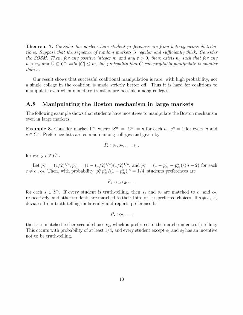
Theorem 7. Consider the model where student preferences are from heterogeneous distribu-tions. Suppose that the sequence of random markets is regular and sufficiently thick. Considerthe SOSM. Then, for any positive integer m and any ε > 0, there exists n0 such that for anyn > n0 and C ⊆ Cn with |C| ≤ m, the probability that C can profitably manipulate is smallerthan ε.

Our result shows that successful coalitional manipulation is rare: with high probability, nota single college in the coalition is made strictly better off. Thus it is hard for coalitions tomanipulate even when monetary transfers are possible among colleges.

A.8 Manipulating the Boston mechanism in large markets

The following example shows that students have incentives to manipulate the Boston mechanismeven in large markets.

Example 8. Consider market Γn, where |Sn| = |Cn| = n for each n. qnc = 1 for every n and

c ∈ Cn. Preference lists are common among colleges and given by

Pc : s1, s2, . . . , sn,

for every c ∈ Cn.

Let pnc1 = (1/2)1/n, pn

c2 = (1 − (1/2)1/n)(1/2)1/n, and pnc = (1 − pn

c1 − pnc2)/(n − 2) for each

c 6= c1, c2. Then, with probability [pnc1

pnc2

/(1 − pnc1

)]n = 1/4, students preferences are

Ps : c1, c2, . . . ,

for each s ∈ Sn. If every student is truth-telling, then s1 and s2 are matched to c1 and c2,respectively, and other students are matched to their third or less preferred choices. If s 6= s1, s2

deviates from truth-telling unilaterally and reports preference list

Ps : c2, . . . ,

then s is matched to her second choice c2, which is preferred to the match under truth-telling.This occurs with probability of at least 1/4, and every student except s1 and s2 has an incentivenot to be truth-telling.

10

B Appendix B: Proofs

B.1 Proof of Theorem 1

We prove Theorem 1 through several steps. Specifically, we prove three key lemmas, Lemmas1, 3 and 7 and then use them to show the theorem. For the proof of Lemmas 1 and 3, we keepthe set of students and colleges fixed, and refer to markets in terms of preference profiles only.

Let (Pc, qc) be a pair of the true preference list and true quota of college c. A report (P ′c, qc)

is said to be a dropping strategy if (i) sPcs′ and sP ′

c∅ imply sP ′cs

′, and (ii) ∅Pcs implies∅P ′

cs. A dropping strategy does not modify quotas and simply declares some students who areacceptable under Pc as unacceptable. It does not change the relative ordering of acceptablestudents or declare unacceptable students as acceptable.

B.1.1 Lemma 1: Dropping strategies are exhaustive

Given a stable mechanism ϕ, denote the matching under ϕ with respect to reported profile(P, q) by ϕ(P, q). The formal statement of Lemma 1 in the main text is as follows.

Lemma 1. Consider an arbitrary stable mechanism ϕ. Fix preference profile (P, q). For somereport (Pc, qc) of c, suppose that ϕ((Pc, P−c), (qc, q−c)) = µ. Then there exists a dropping strategy(P ′

c, qc) such that ϕ((P ′c, P−c), q) �c µ.

Proof. Construct dropping strategy (P ′c, qc) such that P ′

c lists all the students it is matched tounder µ who are acceptable ({s ∈ µ(c)|sPc∅}) in the same relative order as in Pc, and reportsevery other student as unacceptable. Let (P ′, q) = (P ′

c, P−c, q).We will show ϕ(P ′, q)(c) is equal to {s ∈ µ(c)|sPc∅}. This equality implies that ϕ(P ′, q) �c

µ, since ϕ(P ′, q)(c) can only differ from µ(c) in having no unacceptable students under the truepreference list Pc. The proof proceeds in two steps.

First, consider the matching µ′ obtained from µ by having c keep only the students in µ(c)that are acceptable under Pc. That is,

µ′(c′) =

{

{s ∈ µ(c)|sPc∅} c′ = c,

µ(c′) c′ 6= c.

Consider the properties of µ′ under (P ′, q). First, µ′ is individually rational under (P ′, q).Second, there is no blocking pair involving c, since µ′(c) is exactly the set of students acceptableunder P ′

c. However, there may be a blocking pair involving another college and students whoare unmatched. In this case, we can define a procedure which ultimately yields a matching thatis stable under (P ′, q):3

3This procedure parallels Blum, Roth and Rothblum (1997)’s analogous vacancy-chain procedure for one-to-one matching markets and Cantala (2004)’s algorithm for many-to-one markets.

11

Starting from µ′0 ≡ µ′, let S0 be the set of students that can be part of a blocking pair in

µ′0. Pick some s ∈ S0. Let college c′ be the college that student s prefers the most within the

set of colleges that can be part of a blocking pair with s. Construct µ′1 by assigning student s

to c′ and if |µ′0(c

′)| = qc′, then let c′ reject its least preferred student. By construction, µ′1 is

individually rational, college c is matched to the same set of students, college c′ strictly prefersµ′

1(c′) over µ′

0(c′) and the assignments of all other colleges are unchanged. As with µ′

0, the onlyblocking pair of µ′

1 involves unmatched students. If there are blocking pairs of µ′1, then repeat

the same procedure to construct µ′2, and so on.

At each repetition, the new matching is individually rational, college c is matched to thesame set of students, one other college strictly improves and the remaining colleges are notworse off since each blocking pair involves an unassigned student. Since colleges can strictlyimprove only a finite number of times, this procedure terminates in finite time. The ultimatematching µ′′ is stable in (P ′, q) because it is individually rational and there are no blockingpairs. Moreover, since college c obtains the same matching in each repetition,

µ′′(c) = µ′(c). (1)

The second step of the proof utilizes the fact that for any college, the same number ofstudents are matched to it across different stable matchings (Roth 1984a). Since µ′′ is stablein (P ′, q) and ϕ(P ′, q) is stable in (P ′, q) by definition, |µ′′(c)| = |ϕ(P ′, q)(c)|. Since there arejust |µ′′(c)| acceptable students under P ′

c, this implies that

µ′′(c) = ϕ(P ′, q)(c). (2)

Equations (1) and (2) together imply that

ϕ(P ′, q)(c) = µ′(c) = {s ∈ µ(c)|sPc∅}.As a result,

ϕ(P ′, q)(c) �c µ(c),

since ϕ(P ′, q)(c) can only differ from µ(c) in having no unacceptable students under the truepreference list Pc.

B.1.2 Lemma 3: Rejection chains

For preference profile (P, q), let µ be the student-optimal stable matching. Let B1c be an

arbitrary subset of µ(c). The rejection chains algorithm with input B1c is defined as follows.

Algorithm 1. Rejection Chains

(1) Initialization:

12

(a) µ is the student-optimal stable matching, and B1c is a subset of µ(c). Let i = 0. Let

c reject all the students in B1c .

(2) Increment i by one.

(a) If Bic = ∅, then terminate the algorithm.

(b) If not, let s be the least preferred student by c among Bic, and let Bi+1

c = Bic \ s.

(c) Iterate the following steps (call this iteration “Round i”).

i. Choosing the applied:

A. If s has already applied to every acceptable college, then finish the iterationand go back to the beginning of Step 2.

B. If not, let c′ be the most preferred college of s among those which s has notyet applied while running the SOSM or previously within this algorithm. Ifc′ = c, terminate the algorithm.

ii. Acceptance and/or rejection:

A. If c′ prefers each of its current mates to s and there is no vacant position,then c′ rejects s; go back to the beginning of Step 2c.

B. If c′ has a vacant position or it prefers s to one of its current mates, thenc′ accepts s. Now if c′ had no vacant position before accepting s, then c′

rejects the least preferred student among those who were matched to c′. Letthis rejected student be s and go back to the beginning of Step 2c. If c′ hada vacant position, then finish the iteration and go back to the beginning ofStep 2.

Algorithm 1 terminates either at Step 2a or at Step 2(c)iB. We say that Algorithm 1 doesnot return to c if it terminates at Step 2a and it returns to c if it terminates at Step 2(c)iB.

Lemma 2. Consider college c and suppose that under (P, q), Algorithm 1 with every possiblesubset of µ(c) as an input fails to return to c. For any dropping strategy (P ′

c, qc), let B1c = {s ∈

µ(c)|∅P ′cs} be non-empty and let µ′ be a matching obtained at the end of Algorithm 1 with input

B1c . Then, under (P ′

c, P−c, q),

(1) µ′ is individually rational,

(2) no c′ 6= c is a part of a blocking pair of µ′, and

(3) if (s, c) blocks µ′, then [arg minPcµ(c)]Pcs,

4 and

4For any binary relation R on X and X ′ ⊆ X , arg minR X ′ = {x ∈ X ′|yRx for any y ∈ X ′}.

13

(4) if (s, c) blocks µ′ and µ′(c) is non-empty, then [arg minP ′

cµ′(c)]P ′

cs.

Proof. Part (1): For c′ 6= c, c′ only accepts students who are acceptable in each step of theSOSM and Algorithm 1. c rejects every student who is unacceptable under P ′

c at the outset ofAlgorithm 1, and accepts no other student by the assumption that Algorithm 1 does not returnto c for any subset of µ(c) as an input. Therefore µ′ is individually rational.

Part (2): Suppose that for some s ∈ S and c′ ∈ C such that c′ 6= c, c′Psµ′(s). Then, by

the definition of the SOSM and Algorithm 1, s is rejected by c′ either during the SOSM or inAlgorithm 1. This implies that |µ′(c′)| = qc′ and [arg minPc′

µ′(c)]Pc′s, implying that s and c′

do not block µ′.Part (3): Suppose cPsµ

′(s) for some s ∈ S. As in Part (2), this implies that s is rejectedby c either during the SOSM or in Algorithm 1. Since Algorithm 1 does not return to c byassumption, s is rejected either during the SOSM or at the beginning of Algorithm 1. In theformer case, if s is rejected during the SOSM, then [arg minPc

µ(c)]Pcs. In the latter case, (s, c)is not a blocking pair because s is declared unacceptable under P ′

c.Part (4): From Part (3), we have that

[arg minPc

µ(c)]Pcs. (3)

By definition, µ′(c) ⊆ µ(c) and expression (3) imply

[arg minPc

µ′(c)]Pcs, (4)

when µ′(c) is non-empty.When µ′(c) is non-empty, µ′(c) is constructed by including only acceptable students in µ(c)

according to P ′c, so

[arg minP ′

c

µ′(c)]P ′c∅. (5)

Expressions (4) and (5) and the definition of a dropping strategy yield

[arg minP ′

c

µ′(c)]P ′cs.

Lemma 3 (Rejection chains). For any market and any c ∈ C, if Algorithm 1 does not returnto c for any non-empty B1

c ⊆ µ(c), then c cannot profitably manipulate by a dropping strategy.

Proof. Consider an arbitrary dropping strategy (P ′c, qc) and let B1

c = {s ∈ µ(c)|∅P ′cs}. When

Algorithm 1 does not return to c, we show that µ = φ(P, q) is weakly preferred by college c toφ(P ′

c, P−c, q). Let (P ′, q) = (P ′c, P−c, q).

14

Let µ′ be the matching resulting from Algorithm 1 with input B1c . In the first step of the

proof, we construct a new matching µ′′ by satisfying the blocking pairs involving college c suchthat college c weakly prefers µ over µ′′ according to profile (P, q). The second step of the proofshows that µ′′ is weakly preferred to φ(P ′, q) by college c. These two steps together will yieldour desired conclusion.

First, suppose that c does not block µ′ in (P ′, q). Then let µ′′ = µ′. It is clear that college cweakly prefers µ over µ′′ because µ′′(c) = µ′(c) ⊆ µ(c). Otherwise, if c blocks µ′, construct µ′′

as follows: College c admits its most preferred students under P ′c who are willing to be matched

possibly leaving the seats occupied by these students at other colleges vacant; that is,

µ′′(c′) =

{

µ′(c) ∪ arg max(P ′

c,qc−|µ′(c)|){s ∈ S|cPsµ′(s)} c′ = c,

µ′(c′) \ µ′′(c) c′ 6= c,

where arg max(P ′

c,qc−|µ′(c)|) X denotes at most qc −|µ′(c)| students that are most preferred underP ′

c in set X. Recall that µ′(c) ⊆ µ(c) by definition. Moreover, Part (3) of Lemma 2 shows that,under µ′′, |µ′(c)| positions of c are filled with µ′(c) and the remaining |µ′′(c) − µ′(c)| positionsare filled with students less preferred to arg minPc

µ(c). Since preferences are responsive, weobtain

µ(c) �c µ′′(c). (6)

In the second step of the proof, we demonstrate that µ′′ is weakly preferred to φ(P ′, q)by college c. The proof works by comparing µ′′ to a stable matching µ′′′ in (P ′, q), that weconstruct below:

Case 1: If µ′′ is stable in (P ′, q), then let µ′′′ = µ′′. In this case, it is obvious that µ′′(c) is weaklypreferred to µ′′′(c) under P ′

c.

Case 2: Otherwise, observe the following properties of µ′′:

1) Matching µ′′ is individually rational.

2) College c is not part of a blocking pair under µ′′.

3) The only blocking pairs in µ′′ involve colleges who have vacant seats.

Property (1) follows by construction. To establish Property (2), we consider two cases.When µ′(c) is empty, µ′′(c) is college c’s most preferred students according to P ′

c who arepart of blocking pairs of µ′. College c is not part of a blocking pair under µ′′. Whenµ′(c) is not empty, suppose college c is preferred by student s to µ′′(s). In this case, Part(4) of Lemma 2 implies that s is less preferred than any student in µ′(c) under Pc′ andis less preferred than students in arg max(P ′

c,qc−|µ′(c)|){s ∈ S|cPsµ′(s)} by construction.

15

Therefore, college c does not form a blocking pair with this student, and, hence, c is notpart of any blocking pair under µ′′. Finally, Property (3) follows by construction and byPart (2) of Lemma 2.

With these properties in hand, we construct µ′′′. Let µ′′0 ≡ µ′′. µ′′

0 may have a blockingpair involving a college with a vacant seat. Construct µ′′

1 as follows. Let C0 be the set ofcolleges that can be part of a blocking pair in µ′′

0. Pick some c′ ∈ C0. Let student s be thestudent that college c′ prefers the most within the set of students involved in blocking pairswith c′. Construct µ′′

1 by assigning college c′ to s, and if µ′′0(s) 6= ∅, then s rejects µ′′

0(s),leaving a vacant seat at college µ′′

0(s). Under µ′′1, student s receives a strictly preferred

assignment and each other student’s assignment is unchanged. For college c, µ′′1(c) is

weakly less preferred under P ′c than the initial matching, µ′′

0(c), because the students arebetter off in µ′′

1. Matching µ′′1 is individually rational, and as with µ′′

0, the only blockingpair of µ′′

1 involves colleges with vacant seats. If there are blocking pairs of µ′′1, then we

repeat the same procedure to construct µ′′2, and so on.

At each repetition, the new matching is individually rational and each blocking pair of thenew matching involves a college with a vacant seat. As a result, no additional studentsare rejected when the blocking pair is satisfied, and in each repetition, one student strictlyimproves and the remaining students do not change their assignment. Since students mayimprove their assignment a finite number of times, the procedure ends in finite time.

The ultimate matching µ′′′ is stable in (P ′, q) because it is individually rational andthere are no blocking pairs. Moreover, for college c, each new matching is weakly lesspreferred under P ′

c than the initial matching µ′′0(c) as students weakly improve in each

new matching. Hence, µ′′(c) is weakly preferred to µ′′′(c) under P ′c.

Since the matching produced by SOSM is the least preferred stable matching of everycollege (attributed to Conway in Knuth (1976), φ(P ′, q)(c) is weakly less preferred to the stablematching µ′′′ by college c under P ′

c. This implies that φ(P ′, q)(c) is weakly less preferred toµ′′(c) under P ′

c, and since P ′c is a dropping strategy of Pc,

µ′′(c) �c φ(P ′, q)(c). (7)

Equations (6) and (7) together allow us to conclude that

µ(c) �c φ(P ′, q)(c),

showing that (P ′c, qc) is not a profitable strategy when Algorithm 1 does not return to c.

16

B.1.3 Lemma 7: Vanishing market power

We are interested in how often Algorithm 1 returns to a particular college c for the case wherestudents draw their preferences from distribution Dn. Let

πc = Pr[Algorithm 1 returns to c for some B1c ⊆ µ(c)].

Since Algorithm 1 returns to c for some B1c whenever c can manipulate the SOSM (Lemmas

1 and 3), πc gives an upper bound of the probability that c can manipulate the SOSM whenothers are truthful conditional on µ being realized as the matching under the SOSM. Here wewill show Lemma 7, which bounds πc for most colleges in large markets.

Consider the following algorithm, which is a stochastic variant of the SOSM.5

Algorithm 2. Stochastic Student-Optimal Gale-Shapley Algorithm

(1) Initialization: Let l = 1. For every s ∈ S, let As = ∅.

(2) Choosing the applicant:

(a) If l ≤ |S|, then let s be the lth student and increment l by one.6

(b) If not, then terminate the algorithm.

(3) Choosing the applied:

(a) If |As| ≥ k, then return to Step 2.

(b) If not, select c randomly from distribution Dn until c /∈ As, and add c to As.

(4) Acceptance and/or rejection:

(a) If c prefers each of its current mates to s and there is no vacant position, then crejects s. Go back to Step 3.

(b) If c has a vacant position or it prefers s to one of its current mates, then c accepts s.Now if c had no vacant position before accepting s, then c rejects the least preferredstudent among those who were matched to c. Let this student be s and go back toStep 3. If c had a vacant position, then go back to Step 2.

5To be more precise this is a stochastic version of the algorithm proposed by McVitie and Wilson (1970),which they show produces the same matching as the original SOSM proposed by Gale and Shapley (1962).

6Recall that students are ordered in an arbitrarily fixed manner.

17

As records colleges that s has already drawn from Dn. When |As| = k is reached, As is theset of colleges acceptable to s.

Under the SOSM, a student’s application to her tth most preferred college is independent ofher preferences after (t + 1)th choice on. Therefore the above algorithm terminates, producingthe student-optimal stable matching of any realized preference profile which would follow fromcompleting the draws for random preferences. Let µ be the student-optimal stable matchingobtained by the above algorithm.

Suppose that Algorithm 2 is run and the stable matching µ is obtained. Now fix a collegec ∈ C and let B1

c be an arbitrary subset of µ(c). The stochastic rejection chains associatedwith B1

c is defined as follows. As the name suggests, this is a stochastic version of Algorithm 1.

Algorithm 3. Stochastic Rejection Chains

(1) Initialization:

(a) Keep all the preference lists generated in Algorithm 2. Also, for each s ∈ S, let As

be the set generated at the end of Algorithm 2. Let the student-optimal matchingµ be the initial match of the algorithm. Let B1

c be a given subset of µ(c). Let i = 0.Let c reject all the students in B1

c .

(2) Increment i by one.

(a) If Bic = ∅, then terminate the algorithm.

(b) If not, let s be the least preferred student by c among Bic, and let Bi+1

c = Bic \ s.

(c) Iterate the following steps (call this iteration “Round i”.)

i. Choosing the applied:

A. If |As| ≥ k, then finish the iteration and go back to the beginning of Step 2.

B. If not, select c′ randomly from distribution Dn until c′ /∈ As, and add c′ toAs. If c is selected, terminate the algorithm.

ii. Acceptance and/or rejection:

A. If c′ prefers each of its current mates to s and there is no vacant position,then c′ rejects s; go back to the beginning of Step 2c.

B. If c′ has a vacant position or it prefers s to one of its current mates, thenc′ accepts s. Now if c′ had no vacant position before accepting s, then c′

rejects the least preferred student among those who were matched to c′. Letthis rejected student be s and go back to the beginning of Step 2c. If c′ hada vacant position, then finish the iteration and go back to the beginning ofStep 2.

18

Algorithm 3 terminates either at Step 2a or at Step 2(c)iB. Similarly to Algorithm 1, wesay that Algorithm 1 returns to c if it terminates at Step 2(c)iB and does not return to cif it terminates at Step 2a.

We are interested in how often the algorithm returns to c, as a student draws c fromdistribution Dn. It is clear that the probability that Algorithm 1 returns to c is equal to theprobability that Algorithm 3 returns to c. That is,

πc = Pr[Algorithm 3 returns to c for some B1c ⊆ µ(c)].

This latter expression is useful since we can investigate the procedure step by step, utilizingconditional probabilities and conditional expectations. Recall that we have ordered the collegesin terms of decreasing popularity. Our notation is that when c′ ≤ c, we mean that c′ is morepopular than c, or pc′ ≥ pc and when we write c > m, where m is a natural number, we meanthe index of college c is larger than m. Let

Vc = {c′ ∈ Cn|c′ ≤ c, c′ /∈ As for every s ∈ Sn at the end of Algorithm 2}, and

Yc = |Vc|.

Vc is a random set of colleges that are more popular than c ex ante but listed on no student’spreference list at the end of Algorithm 2. Yc is a random variable indicating the number ofsuch colleges.7

Lemma 4. For any c > 4k, we have

E[Yc] ≥c

2e−8qnk/c.

Proof. Let Qn =∑k

c=1 pnc . Then the probability that c′ is not a student’s ith choice, denoted

c(i), given her first (i − 1) choices c(1), . . . , c(i−1) is bounded as follows:

1 − pnc′

1 − ∑i−1j=1 pn

c(j)

≥ 1 − pnc′

1 − Qn.

Let Ec′ be the event that c′ /∈ As for every s ∈ S at the end of Algorithm 2. Since there are atmost qnk draws from Dn in Algorithm 2, the above inequality implies that

Pr(Ec′) ≥(

1 − pnc′

1 − Qn

)qnk

.

7We abuse notation and denote a random variable and its realization by the same letter when there is noconfusion.

19

If c′ > k, there are at least c′ − k colleges that are at least as popular as c′, but not amongthe k most popular colleges, so we obtain

pnc′ ≤

1 − Qn

c′ − k.

The last two inequalities imply

Pr(Ec′) ≥(

1 − 1

c′ − k

)qnk

. (8)

We now show that for any c′ > 2k,

(

1 − 1

c′ − k

)qnk

≥ e−2qnk/(c′−k). (9)

To see this, first note that

(

1 − 1

c′ − k

)qnk

≥ e−2qnk/(c′−k) ⇐⇒ 1 − 1

c′ − k− e−2/(c′−k) ≥ 0.

Now, define a function f(x) = 1 − x − e−2x. This function f is concave, and f(0) = 0 andf(1/2) = 1/2 − 1/e > 0. Therefore f(x) ≥ 0 for any x ∈ [0, 1/2]. Since c′ > 2k and k is apositive integer, we have c′−k > k ≥ 1. Since c′−k is an integer, we thus obtain c′−k ≥ 2 andhence 1/(c′−k) ∈ [0, 1/2]. Therefore 1−1/(c′−k)− e−2/(c′−k) = f(1/(c′−k)) ≥ 0, establishinginequality (9).

Moreover, for any c′ > 2k,

e−2qnk/(c′−k) ≥ e−4qnk/c′. (10)

Combining inequalities (8), (9), and (10), we obtain:

Pr(Ec′) ≥ e−4qnk/c′.

Using the previous inequality, for any c > 4k, we have

E[Yc] =

c∑

c′=1

Pr(Ec′) ≥c

∑

c′=2k

e−4qnk/c′ ≥c

∑

c′=c/2

e−8qnk/c =c

2e−8qnk/c.

20

For B1c ⊆ µ(c), let

πB1c

c = Pr[Algorithm 3 with input B1c returns to c|Yc > E[Yc]/2, µ].

πB1

cc gives an upper bound of the probability that c can manipulate the SOSM when others

are truthful, conditional on two events: µ is the realized matching under the SOSM withtruthful preferences and there are not too small a number of colleges (Yc > E[Yc]/2) that aremore popular than c and appear nowhere on students’ preference lists at the end of Algorithm2.

Let c∗(n) = 16qnk/ ln(qn). We will see, in Lemma 7, that c∗(n) is the number of “verypopular colleges” in a market with n colleges. Note that c∗(n)/n converges to zero as n → ∞,so the proportion of such colleges goes to zero. Except for these c∗(n) colleges, the followinglemma gives an upper bound for manipulability in a large market.

Lemma 5. Suppose that n is sufficiently large and c > c∗(n). Then we have

πB1c

c ≤ 4q

E[Yc],

for any B1c ⊆ µ(c).

Proof. Consider Round 1, beginning with the least preferred student s of B1c ⊆ µ(c) (if B1

c = ∅,then the inequality is obvious since π

B1c

c = 0.). Since pnc′ ≥ pn

c for any c′ ∈ Vc, Round 1 ends atStep 2(c)iiB as a student applies to some college with vacant positions, at least with probability1 − 1/(Yc + 1) > 1 − 1/(E[Yc]/2 + 1).

Now assume that all Rounds 1, . . . , i − 1 end at Step 2(c)iiB. Then there are still atleast Yc − (i − 1) colleges more popular than c and with a vacant position, since at mosti − 1 colleges in Vc have had their positions filled at Rounds 1, . . . , i − 1. Therefore Round iinitiated by the least preferred student in Bi

c ends at Step 2(c)iiB with probability of at least1 − 1/(E[Yc]/2 − (i − 1) + 1). Note that

E[Yc]/2 − (i − 1) + 1 ≥ E[Yc]/4 > 0, (11)

for sufficiently large n. To see this, it is sufficient to show

E[Yc]/4 − (i − 1) + 1 ≥ 0.

Since there are at most q rounds,

E[Yc]/4 − (i − 1) + 1 ≥ E[Yc]/4 − q + 2.

21

The definition of Yc implies that Yc is weakly increasing in c. Lemma 4 provides a lower boundon E[Yc], which for c > c∗(n) implies

E[Yc]/4 − q + 2 ≥ 2qkn12

ln(n)− q + 2,

which is positive for sufficiently large n, showing inequality (11) for sufficiently large n.Since there are at most q rounds, Algorithm 3 fails to return to c with probability of at least

q∏

i=1

(

1 − 1

E[Yc]/2 − (i − 1) + 1

)

≥(

1 − 1

E[Yc]/4

)q

, (12)

for sufficiently large n and c > c∗(n), because of inequality (11).Therefore we have that

πB1c

c ≤ 1 −(

1 − 1

E[Yc]/4

)q

≤ 4q

E[Yc],

where the last inequality holds since 1 − (1 − x)y ≤ yx for any x ∈ (0, 1) and y ≥ 1.8

We state without proof the following lemma (this is a straightforward generalization ofLemma 4.4 of Immorlica and Mahdian (2005)).

Lemma 6. For every c, we have V ar[Yc] ≤ E[Yc].

Now we are ready to present and prove the last of the three key lemmas.

Lemma 7 (Vanishing market power). If n is sufficiently large and c > c∗(n), then

πc ≤[q(2q − 1) + 1] ln(qn)

2k√

qn.

Proof. By the fact that any probability is non-negative and less than or equal to one, theChebychev inequality, and Lemma 6, we have

Pr

[

Yc ≤E[Yc]

2

]

≤ Pr

[

Yc ≤E[Yc]

2

]

+ Pr

[

Yc ≥3E[Yc]

2

]

= Pr

[

|Yc − E[Yc]| ≥E[Yc]

2

]

≤ V ar[Yc]

(E[Yc]/2)2≤ 4

E[Yc].

8Note that conditions for this inequality is satisfied since 4/E[Yc] ∈ (0, 1) for any sufficiently large n andc > c∗(n).

22

Since the probability of a union of events is at most the sum of the probabilities of individualevents (Boole’s inequality), Lemma 5 and the fact that there are at most 2q − 1 non-emptysubsets of µ(c) imply

Pr[Algorithm 3 returns to c for some B1c ⊆ µ(c)|Yc ≥ E[Yc]/2, µ]

≤∑

B1c⊆µ(c)

πB1c

c

≤ 4q(2q − 1)

E[Yc].

This inequality holds for any matching µ. Therefore, we have the same upper bound forprobability conditional on Yc > E[Yc]/2 but not on µ, that is,

Pr

[

Algorithm 3 returns to c for some B1c ⊆ µ(c)|Yc ≥

E[Yc]

2

]

(13)

≤ 4q(2q − 1)

E[Yc]. (14)

By the above inequalities and the fact that probabilities are less than or equal to one,

πc ≤ Pr

[

Yc ≤E[Yc]

2

]

+ Pr

[

Yc >E[Yc]

2

]

× 4q(2q − 1)

E[Yc]

≤ 4

E[Yc]+

4q(2q − 1)

E[Yc]

=4[q(2q − 1) + 1]

E[Yc].

Applying Lemma 4 and noting that E[Yc] is increasing in c so E[Yc∗(n)] ≤ E[Yc] for anyc > c∗(n) = 16qnk/ ln(qk), we complete the proof of Lemma 7.9

B.1.4 Theorem 1

Now we prove Theorem 1. Let

α(n) = E[#{c ∈ C|φ(S, C, (P ′c, P−c), (q

′c, q−c)) ≻c φ(S, C, P, q)

for some (P ′c, q

′c) in the induced market}|Γn],

be the expected number of colleges that can manipulate in the market induced by randommarket Γn under φ when others report preferences truthfully. By Lemma 1, it suffices to consider

9Note that Lemma 4 can be applied since for sufficiently large n and c ≥ c∗(n), we have c > 4k.

23

dropping strategies. By Lemma 3, the probability that c ∈ C can successfully manipulate bysome dropping strategy is at most πc. Thus we obtain

α(n)/n =

[

∑

c∈Cn

Pr[c successfully manipulates]

]

/n

≤ c∗(n)/n + [n

∑

c≥c∗(n)

πc]/n

≤ c∗(n)/n + [n

∑

c≥c∗(n)

[q(2q − 1) + 1] ln(qn)

2k√

qn]/n (by Lemma 7)

≤ 16qk

ln(qn)+

(q(2q − 1) + 1) ln(qn)

2√

qk√

n(by c∗(n) = 16qnk/ ln(qn)).

The first term is proportional to 1/ ln(qn) and the second term is proportional to ln(qn)/√

n.Since both expressions approach zero as n approaches infinity, we obtain α(n)/n → 0 as n → ∞,completing the proof.

B.2 Proof of Theorem 3

In this section, we consider the possibility of pre-arrangement, so we reintroduce S and C asarguments to the mechanism to avoid confusion.

B.2.1 Lemma 8

The following lemma says that a student that is involved in pre-arrangement is less preferredby the college to any student who is matched to it without pre-arrangement.

Lemma 8. If c ∈ C can manipulate via pre-arrangement with s ∈ S, then

s′Pcs for every s′ ∈ φ(S, C, P, q)(c).

Proof. Let µ(c) = φ(S, C, P, q)(c). Theorem 2 of Sonmez (1999) implies that, for any stablemechanism, if c can manipulate via pre-arrangement with student s, then either s ∈ µ(c) ors′Pcs for every s′ ∈ µ(c). To show s /∈ µ(c), suppose on the contrary that s ∈ µ(c). Considermatching µ′ given by

µ′(c′) =

{

µ(c) \ s if c′ = c,

µ(c′) otherwise.

It is easy to see, from stability of µ in (S, C, P, q), that µ′ is stable in (S \ s, C, P−s, qc − 1, q−c).

24

Since the matching under the SOSM is weakly less preferred to any stable matching bycolleges and preferences are responsive,

φ(S, C, P, q)(c) = µ′(c) ∪ s

�c φ(S \ s, C, P−s, qc − 1, q−c)(c) ∪ s.

Therefore c cannot manipulate the student-optimal stable mechanism via pre-arrangement.This is a contradiction, completing the proof.

To profitably manipulate, a college has to pre-arrange a match with a strictly less preferredstudent. Then the disadvantage of being matched with a less desirable student should becompensated by matching to a better set of students in the centralized matching mechanismafter pre-arrangement.

B.2.2 Theorem 3

Now we prove our result on pre-arrangement, Theorem 3. Start with matching φ(S, C, P, q),and consider what happens when college c reduces capacity by one. There are two cases toconsider. First, the capacity reduction may not affect the matching of college c,

φ(S, C, P, qc − 1, q−c)(c) = φ(S, C, P, q)(c).

This happens when |φ(S, C, P, q)(c)| < qc, or the number of students assigned to college c isless than its total capacity. Because there is an extra seat at college c, no student s wouldprefer to be assigned to college c over her matching φ(S, C, P, q)(s) because there would be ablocking pair, which contradicts the stability of φ(S, C, P, q)(s). Therefore, in the first case,pre-arrangement is not successful.

Second, the capacity reduction may affect the matching of college c. In this case,consider the rejection chain algorithm (Algorithm 1) starting with φ(S, C, P, q) with inputB1

c = arg minPcφ(S, C, P, q)(c). We focus on the case where the rejection chain algorithm does

not return to college c. Denote the resulting matching by µ′. Under µ′, college c obtainsφ(S, C, P, q)(c) \ arg minPc

φ(S, C, P, q)(c).

We claim that µ′ is stable in (S, C, P, qc − 1, q−c). The ideas follow from Lemma 2.

First, we claim µ′ is individually rational. For c′ 6= c, c′ only accepts students who areacceptable in each step of the SOSM and Algorithm 1. c is matched to φ(S, C, P, q)(c) \arg minPc

φ(S, C, P, q)(c) at µ′, which is clearly individually rational for c under (Pc, qc−1).Therefore, µ′ is individually rational.

Second, there is no blocking pair of µ′ involving a college other than c. Suppose that forsome s ∈ S and c′ ∈ C such that c′ 6= c, c′Psµ

′(s). Then, by the definition of the SOSM

25

and Algorithm 1, s is rejected by c′ either during the SOSM or in Algorithm 1. Thisimplies that |µ′(c′)| = qc′ and [arg minPc′

µ′(c)]Pc′s, implying that s and c′ do not blockµ′.

Third, there is no blocking pair of µ′ involving college c. Suppose cPsµ′(s) for some s ∈ S.

As in the previous paragraph, this implies that s is rejected by c either during the SOSMor in Algorithm 1. Since Algorithm 1 does not return to c by assumption, s is rejectedeither during the SOSM or at the beginning of Algorithm 1. In the former case, the factthat s is rejected during the SOSM implies that [arg minPc

µ(c)]Pcs, so when college c hascapacity qc − 1, s will not form a blocking pair with student s because the other qc − 1students who are matched to c are more preferred to [arg minPc

µ(c)]. In the latter case,(s, c) is not a blocking pair because the student rejected at the beginning of Algorithm 1is arg minPc

φ(S, C, P, q)(c) by our assumption, the other qc−1 students who are matchedto c are more preferred by college c, and the capacity of college c is qc − 1.

Therefore, µ′ is stable in (S, C, P, qc − 1, q−c).

The least preferred stable matching for colleges in (S, C, P, qc − 1, q−c) is equal toφ(S, C, P, qc − 1, q−c)(c). Therefore, we can conclude that

µ′(c) = φ(S, C, P, q)(c) \ arg minPc

φ(S, C, P, q)(c) �c φ(S, C, P, qc − 1, q−c)(c). (15)

Since every college is made weakly better off under the SOSM when the set of participatingstudents increases (Gale and Sotomayor (1985)), we obtain

φ(S, C, P, qc − 1, q−c) �c φ(S \ s, C, P−s, qc − 1, q−c). (16)

Lemma 7 shows that the rejection chain algorithm (Algorithm 1) does not return withprobability at least 1 − πc. As a result, with probability 1 − πc,

φ(S, C, P, q)(c) �c φ(S, C, P, qc − 1, q−c)(c) ∪ arg minPc

φ(S, C, P, q)(c)

�c φ(S \ s, C, P−s, qc − 1, q−c)(c) ∪ arg minPc

φ(S, C, P, q)(c)

�c φ(S \ s, C, P−s, qc − 1, q−c)(c) ∪ s,

where the first relation follows from (15) and responsiveness of preferences, the second relationfollows from (16) and responsiveness, and the last relationship follows from Lemma 8 andresponsiveness.

Therefore the probability that c benefits via pre-arrangement is at most πc. Finally, byLemma 7 we complete the proof (this last argument is similar to the one for Theorem 1 andhence omitted).

26

B.3 Proof of Theorems 2 and 5

Since Theorem 5 is a multi-region generalization of Theorem 2, we prove only the former.

B.3.1 Lemma 10: Uniform vanishing market power

We have a variant of Lemma 7 under the sufficient thickness assumption, which plays a crucialrole in the proof of the theorems.

For B1c ⊆ µ(c), let

πB1c

c = Pr[Algorithm 3 associated with B1c returns to c|YT (n) > E[YT (n)]/2, µ].

First we show a variant of Lemma 5.

Lemma 9. Suppose (Γ1, Γ2, . . . ) is regular and sufficiently thick. Let T be such that E[YT (n)] →∞ as n → ∞. Suppose that n is sufficiently large. Then we have

πB1c

c ≤ 4T q

E[YT (n)],

for any c and B1c ⊆ µ(c).

Proof. Consider Round 1, beginning with the least preferred student s of B1c ⊆ µ(c) (if B1

c = ∅,then the inequality is obvious since π

B1c

c = 0.). Since pnc′(r) ≥ pn

c (r)/T for any c′ ∈ VT (n)and r = 1, . . . , R, Round 1 ends at 2(c)iiB as a student applies to some college with vacantpositions, at least with probability 1 − 1/(YT (n)/T + 1) > 1 − 1/(E[YT (n)]/2T + 1).

Now assume that all Rounds 1, . . . , i − 1 end at Step 2(c)iiB. Then there are still at leastYT (n) − (i − 1) colleges more popular than c and with a vacant position, since at most i − 1colleges in VT (n) have had their positions filled at Rounds 1, . . . , i − 1. Therefore Round iinitiated by the least preferred student in Bi

c ends at Step 2(c)iiB with probability of at least1−1/(E[YT (n)]/2T − (i−1)+1). Since there are at most q rounds, Algorithm 3 fails to returnto c with probability of at least

q∏

i=1

(

1 − 1

E[YT (n)]/2T − (i − 1) + 1

)

≥(

1 − 1

E[YT (n)]/2T − q + 2

)q

≥(

1 − 1

E[YT (n)]/4T

)q

.

The first inequality follows since (Γ1, Γ2, . . . ) is sufficiently thick, n is sufficiently large andi ≤ q for each i. The second inequality holds since E[YT (n)]/2 − q ≥ E[YT (n)]/4 > 0, which

27

follows since (Γ1, Γ2, . . . ) is sufficiently thick and n is sufficiently large. Therefore we have that

πB1c

c ≤ 1 −(

1 − 1

E[YT (n)]/4T

)q

≤ 4T q

E[YT (n)],

where the last inequality holds since 1 − (1 − x)y ≤ yx for any x ∈ (0, 1) and y ≥ 1.

Lemma 10 (Uniform vanishing market power). Suppose that (Γ1, Γ2, . . . ) is regular and suffi-ciently thick. For any sufficiently large n and any c ∈ C, we have

πc ≤4 [T q(2q − 1) + 1]

E[YT (n)].

Proof. By Lemma 9 and an argument similar that which leads to expression (13) in Lemma 7,we obtain

Pr[Algorithm 3 returns to c|YT (n) > E[YT (n)]/2] ≤ 4T q(2q − 1)

E[YT (n)].

Therefore we have

πc ≤ Pr [YT (n) ≤ E[YT (n)]/2] + Pr [YT (n) > E[YT (n)]/2] × 4T q(2q − 1)

E[YT (n)]

≤ 4

E[YT (n)]+

4T q(2q − 1)

E[YT (n)]

≤ 4 [T q(2q − 1) + 1]

E[YT (n)],

completing the proof.

B.3.2 Theorems 2 and 5

We only prove Theorem 5, since Theorem 2 is a special case when R = 1. Suppose that collegesother than c are truth-telling, that is, any c′ 6= c reports (Pc′, qc′). Lemmas 1 and 3 apply heresince they do not rely on assumptions about student preferences. These lemmas imply that theprobability that c profitably manipulates is at most πc. By Lemma 10 and sufficient thickness,for any ε > 0, there exists n0 such that for any market Γn with n > n0, we have

Pr [u(φ(S, C, P ′c, P−c, q)(c)) > u(φ(S, C, P, q)(c)) for some P ′

c] <ε

q supn∈N,s∈Sn,c∈Cn uc(s).

28

Such n0 can be chosen independent of c ∈ Cn. For any n > n0, for any c ∈ Cn we have

Euc(φ(S, C, (P ′c, P−c), (q

′c, q−c))(c)) − Euc(φ(S, C, P, q))

<Pr [uc(φ(S, C, (P ′c, P−c), (q

′c, q−c))(c) > uc(φ(S, C, P, q)(c))] q sup

n∈N,s∈Sn,c∈Cn

uc(s)

<ε,

which implies that truthful reporting is an ε-Nash equilibrium.

B.4 Proofs of Propositions 1 and 2

B.4.1 Proposition 1

Let a and T satisfy the condition of nonvanishing proportion of popular colleges. Let c = [an].Then it is obvious that Vc ⊆ VT (n) and hence Yc ≤ YT (n). For sufficiently large n, Lemma 4shows that

E[YT (n)] ≥ E[Yc] ≥c

2e−8qnk/c.

c = [an] implies that c2e−8qnk/c → ∞ as n → ∞ with the order O(n). Therefore E[YT (n)] → ∞

as n → ∞, completing the proof.For Example 5, let c = [γn/ ln(n)]. Substituting into c

2e−8qnk/c, we obtain

E[YT (n)] ≥ c

2e−8qnk/c ≥

[

γn/ ln(n) − 1

2

]

n−8qk

γ =γn1− 8qk

γ

2 ln(n)− 1

2n− 8qk

γ .

Therefore, for γ > 8qk, then n1− 8qk

γ / ln(n) → ∞ and n− 8qk

γ → 0 as n → ∞. Thus, we concludethat E[YT (n)] → ∞ as n → ∞.

B.4.2 Proposition 2

LetV ∗

T (n) = {c ∈ Cn|pn1 (r)/pn

c (r) ≤ T for all r ∈ {1, ..., R}}.Then we have VT (n) = {c ∈ V ∗

T (n) : |{s ∈ Sn|cPss}| < qc}. Let ηr(c) = |{c′ ∈ Cn|pnc (r) ≤

pnc′(r)}| be the order of c with respect to popularity in distribution Dn(r). For example, if

college c is the most popular among students in region 1 and the least popular among those inregion 2, then η1(c) = 1 and η2(c) = n.

Part (1): Example 6. Let T = 4, for example. Then, V ∗4 (n) = {n/4, n/4 + 1, . . . , 3n/4}.

Consider any college c ∈ V ∗4 (n). Let s belong to region r ∈ {1, 2}. Since s picks colleges k times

29

according to Dn(r), the probability that c does not appear in the preference list of student s,denoted by Pr(Fc,s), is bounded as follows:

Pr(Fc,s) ≥(

1 − pnc (r)

1 − Qn(r)

)k

,

whereQn(r) =

∑

c:ηr(c)≤k

pnc (r).

For any sufficiently large n, we have that ηr(c) > 2k for any c ∈ V ∗4 (n) and r = 1, 2 since

[n − 2k] > 3n/4 > c > n/4 > 2k. For such colleges,

pnc (r) ≤ 1 − Qn(r)

ηr(c) − k≤ 1 − Qn(r)

ηr(c)/2.

So

Pr(Fc,s) ≥(

1 − 2

ηr(c)

)k

.

Since ηr(c) ≥ n/4 for any c ∈ V ∗4 (n) and any r = 1, 2, we have

Pr(Fc,s) ≥(

1 − 8

n

)k

.

Let Ec be the event that c is not listed by any student. Then, since students draw collegesindependently, we have

Pr(Ec) =∏

s∈Sn

Pr(Fc,s) ≥ (1 − 8/n)kqn → e−8kq,

as n → ∞. Therefore,

E[YT (n)] =∑

c∈V ∗

4 (n)

Pr(Ec) ≥n

2(1 − 8/n)kqn → ∞,

as n → ∞ (with the order O(n)), completing the proof.Part (2): Example 7. As discussed in Example 7, for any colleges c and c′ and region r,

we have thatpn

c (r)/pnc′(r) = pr(c)(r)/pr(c′)(r) > 0.

Since there are only finite regions, V ∗T (n) = Cn for any sufficiently large T . Fix such T .

30

As in the proof of Part (1), for any c and s we have

Pr(Fc,s) ≥[

1 − pnc (r(s))

1 − Qn(r(s))

]k

.

Since we have that pnc (r)/p

nc′(r) < T for any c, c′ ∈ Cn,

pnc (r)

1 − Qn(r)≤ pn

c (r)

(n − k)pnc (r)/T

≤ 2T

n,

for any sufficiently large n. So we have

Pr(Ec) =∏

s∈Sn

Pr(Fc,s) ≥∏

s∈Sn

(

1 − 2T

n

)k

≥ (1 − 2T/n)kqn → e−2kqT ,

as n → ∞. Therefore

E[YT (n)] =∑

c∈Cn

Pr(Ec)

approaches infinity with the order O(n), completing the proof.

Remark 1. In Examples 4, 6 and 7, the order of convergence of E[YT (n)] is O(n). This impliesthat, by Lemma 10, the order of convergence of the probability of profitable manipulation isO(1/n). This is the same order as in the uniform distribution case, analyzed by Roth andPeranson (1999) and Immorlica and Mahdian (2005).

B.5 Proof of Theorem 7: Coalitional manipulation

The proof is based on a series of arguments similar to those for Theorem 1. First, droppingstrategies are exhaustive for manipulations involving a coalition of agents.

Lemma 11 (Dropping strategies are exhaustive for coalitional manipulations). Consider an ar-bitrary stable mechanism ϕ. Fix preference profile (P, q) and let C ⊆ C be a coalition of colleges.For some arbitrary report (PC , qC) by this coalition, suppose that ϕ((PC , P−C), (qC , q−C)) = µ.Then there exists a dropping strategy (P ′

C, qC) = (P ′

c, qc)c∈C such that ϕ((P ′C, P−C), q) �c µ for

each c ∈ C.

Proof. For each c ∈ C, construct dropping strategy (P ′c, qc) such that P ′

c lists all the studentsit is matched to under µ who are acceptable ({s ∈ µ(c)|sPc∅}) in the same relative order as inPc, and reports every other student as unacceptable. Let (P ′, q) = (P ′

C, P−C , q).

31

We will show ϕ(P ′, q)(c) is equal to {s ∈ µ(c)|sPc∅} for each c ∈ C. This equality impliesthat ϕ(P ′, q) �c µ for each c ∈ C, since ϕ(P ′, q)(c) can only differ from µ(c) in having nounacceptable students under the true preference list Pc. The proof proceeds in two steps.

First, consider the matching µ′ obtained from µ by having each c ∈ C keep only the studentsin µ(c) that are acceptable under Pc. That is,

µ′(c) =

{

{s ∈ µ(c)|sPc∅} c ∈ C,

µ(c) c 6∈ C.

Consider the properties of µ′ under (P ′, q). First, µ′ is individually rational under (P ′, q).Second, there is no blocking pair involving any c ∈ C, since µ′(c) is exactly the set of studentsacceptable under P ′

c. However, there may be a blocking pair involving another college andstudents who are unmatched. In this case, we can define a procedure which ultimately yields amatching that is stable under (P ′, q):

Starting from µ′0 ≡ µ′, let S0 be the set of students that can be part of a blocking pair in µ′

0.Pick some s ∈ S0. Let college c′ be the college that the student s prefers the most within theset of colleges involved in blocking pairs with s. Construct µ′

1 by assigning student s to c′ andif |µ′

0(c′)| = qc′, then let c′ reject its least preferred student. By construction, µ′

1 is individuallyrational, college c is matched to the same set of students, college c′ strictly prefers µ′

1(c′) over

µ′0(c

′) and the assignments of all other colleges are unchanged. As with µ′0, the only blocking

pair of µ′1 involves unmatched students. If there are blocking pairs of µ′

1, then we repeat thesame procedure to construct µ′

2, and so on.At each repetition, the new matching is individually rational, each college c ∈ C is matched

to the same set of students, one other college strictly improves and the remaining colleges arenot worse off since each blocking pair involves an unassigned student. Since colleges can strictlyimprove only a finite number of times, this procedure terminates in finite time. The ultimatematching µ′′ is stable in (P ′, q) because it is individually rational and there are no blockingpairs. Moreover, since each college c ∈ C obtains the same matching in each repetition,

µ′′(c) = µ′(c), for each c ∈ C. (17)

The second step of the proof utilizes the fact that for any college, the same number ofstudents are matched to it across different stable matchings. Since µ′′ is stable in (P ′, q) andϕ(P ′, q) is stable in (P ′, q) by definition, |µ′′(c)| = |ϕ(P ′, q)(c)|, for each c ∈ C. Since for eachc ∈ C, there are just |µ′′(c)| acceptable students under P ′

c, this implies that

µ′′(c) = ϕ(P ′, q)(c), for each c ∈ C. (18)

Equations (17) and (18) together imply that for each c ∈ C,

ϕ(P ′, q)(c) = µ′(c) = {s ∈ µ(c)|sPc∅}.

32

As a result, for each c ∈ Cϕ(P ′, q)(c) �c µ(c),

since ϕ(P ′, q)(c) can only differ from µ(c) in having no unacceptable students under the truepreference list Pc.

B.5.1 Lemma 13: Rejection chains with coalitions

For preference profile (P, q), let µ be the student-optimal stable matching. Let B1c be an

arbitrary subset of µ(c). The rejection chains algorithm with input (B1c )c∈C is defined as

follows.

Algorithm 4. Rejection Chains with Coalitions

(1) Initialization: µ is the student-optimal stable matching µ, input (B1c )c∈C , C1 = C, and

let j = 0.

(2) Algorithm:

(a) Increment j by one (iterate through colleges).

i. If Cj = ∅, then terminate the algorithm.

ii. If not, pick some c ∈ Cj, and let Cj+1 = Cj \ c and let i = 0.

(b) Increment i by one (iterate through students)

i. If Bic = ∅, then go to beginning of Step 2a.

ii. If not, let s be the least preferred student by c among Bic, and let Bi+1

c = Bic \ s.

iii. Iterate the following steps (call this iteration “Round i”).

Choosing the applied:

A. If s has already applied to every acceptable college, then finish the iterationand go back to the beginning of Step 2b.

B. If not, let c′ be the most preferred college of s among those which s has notyet applied while running the SOSM or previously within this algorithm. Ifc′ ∈ C, terminate the algorithm.

Acceptance and/or rejection:

A. If c′ prefers each of its current mates to s and there is no vacant position,then c′ rejects s; go back to the beginning of Step 2(b)iii.

33

B. If c′ has a vacant position or it prefers s to one of its current mates, thenc′ accepts s. Now if c′ had no vacant position before accepting s, then c′

rejects the least preferred student among those who were matched to c′. Letthis rejected student be s and go back to the beginning of Step 2(b)iii. If c′

had a vacant position, then finish the iteration and go back to the beginningof Step 2b.

Algorithm 4 terminates either at Step 2(a)i or at Step 2(b)iiiB. We say that Algorithm 4does not return to C if it terminates at Step 2(a)i and it returns to C if it terminates atStep 2(b)iiiB.

Lemma 12. Consider coalition C and suppose that under (P, q), Algorithm 4 with each possiblecollection of sets consisting of subsets of µ(c) for each c ∈ C as an input fails to return to C.For any dropping strategy (P ′

C, qC), let B1

c = {s ∈ µ(c)|∅P ′cs} for each c ∈ C such B1

c 6= ∅ forat least one c ∈ C, and let µ′ be a matching obtained at the end of Algorithm 4 with input(B1

c )c∈C. Then, under (P ′C, P−C , q),

(1) µ′ is individually rational,

(2) no c 6∈ C is a part of a blocking pair of µ′, and

(3) for c ∈ C, if (s, c) blocks µ′, then [arg minPcµ(c)]Pcs, and

(4) for c ∈ C, if (s, c) blocks µ′ and µ′(c) is non-empty, then [arg minP ′

cµ′(c)]P ′

cs.

Proof. Part (1): For c 6∈ C, c only accepts students who are acceptable in each step of theSOSM and Algorithm 4. Each c ∈ C rejects every student who is unacceptable under P ′

Cat

the outset of Algorithm 4, and accepts no other student by the assumption that Algorithm 4does not return to c ∈ C for any sequence of sets consisting of subsets of µ(c) for each c ∈ Cas input. Therefore µ′ is individually rational.

Part (2): Suppose that for some s ∈ S and c ∈ C \ C, cPsµ′(s). Then, by the definition of

the SOSM and Algorithm 4, s is rejected by c either during the SOSM or in Algorithm 4. Thisimplies that |µ′(c)| = qc and [arg minPc

µ′(c)]Pcs, implying that s and c do not block µ′.Part (3): Suppose cPsµ

′(s) for some s ∈ S and c ∈ C. As in Part (2), this implies that s isrejected by c either during the SOSM or in Algorithm 4. Since Algorithm 4 does not return toc by assumption, s is rejected either during the SOSM or at the beginning of Algorithm 4. Inthe former case, if s is rejected during the SOSM, then [arg minPc

µ(c)]Pcs. In the latter case,(s, c) is not a blocking pair because s is declared unacceptable under P ′

c.Part (4): From Part (3), for each c ∈ C, we have that

[arg minPc

µ(c)]Pcs. (19)

34

By definition, µ′(c) ⊆ µ(c) and expression (19) imply

[arg minPc

µ′(c)]Pcs, (20)

when µ′(c) is non-empty.When µ′(c) is non-empty, µ′(c) is constructed by including only acceptable students in µ(c)

according to P ′c, so

[arg minP ′

c

µ′(c)]P ′c∅. (21)

Expressions (20) and (21) and the definition of a dropping strategy yield

[arg minP ′

c

µ′(c)]P ′cs.

Lemma 13 (Rejection chains with coalitions). For any market and any C ⊆ C, if Algorithm 4does not return to C with each possible collection of sets (B1

c )c∈C, where B1c is a subset of µ(c)

for each c ∈ C, as input (with at least one B1c non-empty), then C cannot profitably manipulate

by a dropping strategy.

Proof. Consider an arbitrary dropping strategy (P ′C, qC) and let B1

c = {s ∈ µ(c)|∅P ′cs} for each

c ∈ C. When Algorithm 4 does not return to C, we show that µ = φ(P, q) is weakly preferredby each college c ∈ C to φ(P ′

C, P−C , q). Let (P ′, q) = (P ′

C, P−C , q).

Let µ′ be the matching resulting from Algorithm 4 with input (B1c )c∈C . The first step of

the proof constructs a new matching µ′′ by satisfying the blocking pairs in µ′ such that µ′′ isstable in (P ′, q)).

We construct µ′′ from µ′ as follows. Parts (1) and (2) of Lemma 12 imply that µ′ isindividually rational and no c 6∈ C is part of a blocking pair of µ′. Parts (3) and (4) of Lemma12 states that if there is a blocking pair involving some c ∈ C, then the student involved in theblocking pair is less preferred than any student in µ(c) under Pc and less preferred than anystudent in µ′(c) under P ′

c.Let µ′′

0 = µ′. Begin by selecting some college c ∈ C involved in a blocking pair of µ′′0.

Construct matching µ′′1 by assigning college c its most preferred students in blocking pairs

up to capacity. The resulting matching is individually rational, at least one student strictlyimproves over µ′′

0, no other student is made worse off, and every blocking pair of µ′′1 involves a

college with a vacant seat. Finally, since students are made weakly better off in µ′′1 than in µ′′

0,it must be the case that if (s, c) blocks µ′′

1, then arg minPcµ(c)Pcs and arg minP ′

cµ′(c)P ′

cs.Next, we construct µ′′

2 by selecting college c who is involved in a blocking pair of µ′′1. Note

that this can either be a college in C or not, but the college that is selected must have a vacant

35

seat. As before, we assign c the most preferred students it forms a blocking pair with up tocapacity. As before, the resulting matching is individually rational, at least one student strictlyimproves over µ′′

1, no other student is made worse off, and every blocking pair of µ′′2 involves a

college with a vacant seat. Finally, since students are made weakly better in µ′′2 than in µ′′

1, itmust be the case that if (s, c) blocks µ′′

2, then arg minPcµ(c)Pcs and arg minP ′

cµ′(c)Pcs.

We repeat this process to construct µ′′3, and so on.

In each step of this construction, no additional students are rejected when we satisfy ablocking pair, and in each step, at least one student strictly improves and the remaining studentsare not made worse off. Since students may improve their assignment only a finite number oftimes, the procedure ends in finite time.

The ultimate matching µ′′ is stable in (P ′, q) because it is individually rational and thereare no blocking pairs. Moreover, for college c, each new student matched to college c is weaklyless preferred under P ′

c than any student in the initial matching µ′′0(c) as students obtain a

weakly more preferred college in each step. Hence, µ′(c) is weakly less preferred to µ′′(c) underP ′

c. Also, for college c, each new student matched to college c is weakly less preferred under Pc

than any student in the matching µ(c) because students obtain a weakly more preferred collegein each step. Thus, µ′′(c) is weakly less preferred to µ(c) under Pc.

Since the matching produced by SOSM is the least preferred stable matching of every college,φ(P ′, q)(c) is weakly less preferred to the stable matching µ′′ by each college c ∈ C in (P ′, q).This will imply that φ(P ′, q)(c) is weakly less preferred to µ′′(c) under P ′

c for each c ∈ C, andsince P ′

c is a dropping strategy of Pc,

µ′′(c) �c φ(P ′, q)(c), for each c ∈ C.

B.5.2 Lemma 14: Uniform vanishing market power for coalitions

For the coalitions, we define

πc = Pr[Algorithm 4 returns to C for some (B1c )c∈C ⊆ ∪c∈Cµ(c)].

Lemma 14. Suppose that (Γ1, Γ2, . . . ) is regular and sufficiently thick. For any sufficientlylarge n and coalition C ⊆ C, we have

πC ≤ 4[

T q · |C| · (2q·|C| − 1) + 1]

E[YT (n)].

Proof. The proof follows exactly the steps leading to Lemma 10 with two modifications. Thefirst modification replaces the first instance of q in the expression in Lemma 10 with q · |C|

36

because in the proof that corresponds to Lemma 9 we must allow for the possibility of q roundsfor each of the |C| colleges. The second modification replaces 2q in the expression in Lemma10 with 2q·|C| because in the proof that corresponds to Lemma 7, there are at most 2q·|C| − 1non-empty subsets of ∪c∈Cµ(c).

Finally, the proof of Theorem 7 follows because in sufficiently thick markets E[YT (n)] → ∞as n → ∞ and |C| ≤ m, so πC → 0.

37

References

Abdulkadiroglu, Atila and Tayfun Sonmez, “School Choice: A Mechanism DesignApproach,” American Economic Review, 2003, 93, 729–747., Parag A. Pathak, Alvin E. Roth, and Tayfun Sonmez, “The Boston Public

School Match,” American Economic Review, Papers and Proceedings, 2005, 95, 368–371., , , and , “Changing the Boston School Choice Mechanism,” 2006. NBER

Working paper, 11965., , and , “The New York City High School Match,” American Economic Review,

Papers and Proceedings, 2005, 95, 364–367., , and , “Strategy-proofness versus Efficiency in Matching with Indifferences:

Redesigning the New York City High School Match,” 2008. forthcoming, AmericanEconomic Review.

Alcalde, Jose and Salvador Barbera, “Top Dominance and the Possibility ofStrategy-Proof Stable Solutions to Matching Problems,” Economic Theory, 1994, 4,417–435.

Blum, Yosef, Alvin E. Roth, and Uriel Rothblum, “Vacancy Chains and Equilibrationin Senior-Level Labor Markets,” Journal of Economic Theory, 1997, 76, 362–411.

Bogomolnaia, Anna and Herve Moulin, “A New Solution to the Random AssignmentProblem,” Journal of Economic Theory, 2001, 100, 295–328.

Bulow, Jeremy and Jonathan Levin, “Matching and Price Competition,” AmericanEconomic Review, 2006, 96, 652–668.

Cantala, David, “Restabilizing Markets at Senior Level,” Games and Economic Behavior,2004, 48, 1–17.

Cripps, Martin and Jeroen Swinkels, “Depth and Efficiency of Large Double Auctions,”Econometrica, 2006, 74, 47–92.

Day, Robert and Paul Milgrom, “Core-Selecting Auctions,” International Journal ofGame Theory, 2008, 36, 393-407.

Demange, Gabrielle, David Gale, and Marilda A. O. Sotomayor, “A Further Note onthe Stable Matching Problem,” Discrete Applied Mathematics, 1987, 16, 217–222.

Dubins, Lester E. and David A. Freedman, “Machiavelli and the Gale-Shapleyalgorithm,” American Mathematical Monthly, 1981, 88, 485–494.

Ehlers, Lars, “In Search of Advice for Participants in Matching Markets which use theDeferred Acceptance Algorithm,” Games and Economic Behavior, 2004, 48, 249–270.

Erdil, Aytek and Haluk Ergin, “What’s the Matter with Tie-Breaking? ImprovingEfficiency in School Choice,” American Economic Review, 2008, 98(3), 669-689.

Ergin, Haluk and Tayfun Sonmez, “Games of School Choice under the BostonMechanism,” Journal of Public Economics, 2006, 90, 215–237.

Fudenberg, Drew, Markus Mobius, and Adam Szeidl, “Existence of Equilibria in

38

Large Double Auctions,” Journal of Economic Theory, 2007, 133, 550–567.Gale, David and Lloyd S. Shapley, “College Admissions and the Stability of Marriage,”

American Mathematical Monthly, 1962, 69, 9–15.and Marilda A. Oliveira Sotomayor, “Some Remarks on the Stable Matching

Problem,” Discrete Applied Mathematics, 1985, 11, 223–232.Gresik, Thomas and Mark Satterthwaite, “The Rate at Which a Simple Market

Converges to Efficiency as the Number of Traders Increases,” Journal of Economic Theory,1989, 48, 304–332.

Haeringer, Guillaume and Flip Klijn, “Constrained School Choice,” 2007. UAB,Unpublished mimeo.

Hatfield, John and Paul Milgrom, “Matching with Contracts,” American EconomicReview, 2005, 95, 913–935.

Immorlica, Nicole and Mohammad Mahdian, “Marriage, Honesty, and Stability,”SODA, 2005, 53–62.

Kelso, Alexander and Vincent Crawford, “Job Matching, Coalition Formation, andGross Substitutes,” Econometrica, 1982, 50, 1483–1504.

Kesten, Onur, “On Two Kinds of Manipulation for School Choice Problems,” 2006.Unpublished mimeo.

Klaus, Bettina and Flip Klijn, “Stable Matchings and Preferences of Couples,” Journal ofEconomic Theory, 2005, 121, 75–106.

Knuth, Donald E., Marriage Stables, Montreal: Les Presse de l’Universite de Montreal,1976., Rajeev Motwani, and Boris Pittel, “Stable Husbands,” Random Structures and

Algorithms, 1990, 1, 1–14.Kojima, Fuhito, “Mixed Strategies in Games of Capacity Manipulation in Hospital-Intern

Markets,” Social Choice and Welfare, 2006, 27, 25–28., “Finding All Stable Matchings with Couples,” 2007a. mimeo., “When can Manipulations be Avoided in Two-Sided Matching Markets? Maximal

Domain Results,” Contributions to Theoretical Economics, 2007b, 7, Article 32.and Mihai Manea, “Strategy-Proofness of the Probabilistic Serial Mechanism in Large

Random Assignment Problems,” 2006. Unpublished mimeo, Harvard University.Konishi, Hideo and Utku Unver, “Games of Capacity Manipulation in the

Hospital-Intern Market,” Social Choice and Welfare, 2006, 27, 3–24.Ma, Jinpeng, “Stable Matchings and the Small Core in Nash Equilibrium in the College

Admissions Problem,” Review of Economic Design, 2002, 7, 117–134.McVitie, D. G. and L. B. Wilson, “Stable Marriage Assignments for Unequal Sets,” BIT,

1970, 10, 295–309.Milgrom, Paul R., Putting Auction Theory to Work, Cambridge: Cambridge University

Press, 2004.

39

Niederle, Muriel, “Competitive Wages in a Match with Ordered Contracts,” AmericanEconomic Review, 2007, 97, 1957–1969.

Pathak, Parag A. and Tayfun Sonmez, “Leveling the Playing Field: Sincere andSophisticated Players in the Boston Mechanism,” American Economic Review, 2008, 98,1636-1652.

Pesendorfer, Wolfgang and Jeroen Swinkels, “Efficiency and Information Aggregationin Auctions,” American Economic Review, 2000, 90, 499–525.

Romero-Medina, Antonio, “Implementation of Stable Solutions in a Restricted MatchingMarket,” Review of Economic Design, 1998, 3, 137–147.

Roth, Alvin E., “The Economics of Matching: Stability and Incentives,” Mathematics ofOperations Research, 1982, 7, 617–628., “The Evolution of the Labor Market for Medical Interns and Residents: A Case Study in

Game Theory,” Journal of Political Economy, 1984a, 92, 991–1016., “Misrepresentation and Stability in the Marriage Problem,” Journal of Economic Theory,

1984b, 34, 383–387., “The College Admission Problem is not Equivalent to the Marriage Problem,” Journal of

Economic Theory, 1985, 36, 277–288., “The Economist as Engineer: Game Theory, Experimentation, and Computation as

Tools for Design Economics, Fisher-Schultz Lecture,” Econometrica, 2002, 70, 1341–1378., “Deferred Acceptance Algorithms: History, Theory, Practice and Open Questions,”

International Journal of Game Theory, 36: 537-569.and Elliot Peranson, “The Redesign of the Matching Market for American Physicians:

Some Engineering Aspects of Economic Design,” American Economic Review, 1999, 89,748–780.and John Vande Vate, “Incentives in Two-sided Matching with Random Stable

Mechanisms,” Economic Theory, 1991, 1, 31–44.and Marilda A. O. Sotomayor, Two-sided Matching: a Study in Game-theoretic

Modeling and Analysis, Cambridge: Econometric Society monographs, 1990.and Uriel Rothblum, “Truncation Strategies in Matching Markets: In Search of Advice

for Participants,” Econometrica, 1999, 67, 21–43., Tayfun Sonmez, and Utku Unver, “Kidney Exchange,” Quarterly Journal of

Economics, 2004, 119, 457–488., , and , “Efficient Kidney Exchange: Coincidence of Wants in Markets with

Compatibility-Based Preferences,” American Economic Review, 2007, 97, 828–851.Rustichini, Aldo, Mark Satterthwaite, and Steven Williams, “Convergence to

Efficiency in a Simple Market with Incomplete Information,” Econometrica, 1994, 62,1041–1064.

Sonmez, Tayfun, “Manipulation via Capacities in Two-Sided Matching Markets,” Journalof Economic Theory, 1997a, 77, 197–204.

40

, “Games of Manipulation in Marriage Problems,” Games and Economic Behavior, 1997b,20, 169–176., “Can Pre-arranged Matches be Avoided in Two-Sided Matching Markets?,” Journal of

Economic Theory, 1999, 86, 148–156.Swinkels, Jeroen, “Efficiency of Large Private Value Auctions,” Econometrica, 2001, 69,

37–68.

41