2INBREEDING, FINITE POPULATION SIZE,

AND GENE FREQUENCY CHANGE

Rough Draft Version 31 July 1998

c©1998 B. Walsh and M. Lynch

Please report errors to jbwalsh@u.arizona.edu

Mating is rarely, if ever, completely random in natural populations. The propagules ofmany species settle down in close proximity to their site of birth, and when mature, tendto mate with other nearby, somewhat-related individuals. This is supported by a numberof investigations that have used genetic markers to track pollen flow in plants. In mostherbaceous species, the vast majority of successful pollinations occur within 10 meters ofthe donor plant (Figure 1). This is almost always a much smaller area than the total rangeof the population. Effective gene flow away from a parent plant can be facilitated by self-incompatibility systems and by elevated mortality of seeds and seedlings near their parentalsource (Levin and Kerster 1974, Levin 1984). Nevertheless, there is little question that theassumption of random mating often made in population-genetic theory is violated to somedegree in all populations. This tendency to mate with individuals with similar genotypes,no matter how minor, is referred to as inbreeding.

The spatial structure of populations is only one of several factors influencing the extentof inbreeding. Even if mating is completely random, there will still be some tendency tomate with relatives since all populations are finite in size. The smaller the population size,the greater this tendency will be. Thus, in a dioecious population with a stable size oftwo, all matings must be between full-sibs, even though the reproductive pair itself may berandom. It follows that the genetic consequences of finite population size must be similarto those of inbreeding.

Inbreeding and finite population size have important effects on gene and genotypefrequencies. In small randomly mating populations, heterozygosity is lost as gamete sam-pling causes allele frequencies to drift towards zero or one. Such random genetic driftof gene frequencies is of negligible importance in very large populations, but the level ofhomozygosity can nevertheless be inflated by consanguineous mating. Subdivision of apopulation into partially isolated demes also results in an increase in the variation in genefrequency between subgroups due to sampling error. The greater the degree of isolation ofthe subgroups, the more pronounced this differentiation will be.

2 CHAPTER 1

Figure 1. Effective gene flow via pollen for four species of herbaceous plants. In each study,visible or electrophoretic markers were scored in the progeny of a large number of plantssurrounding a central (marked) individual. These plots do not completely describe “pollenshadows,” which are usually asymmetrical.

This chapter focuses on the aspects of population structure that influence the rate andmagnitude of gene frequency change in finite populations. For the time being, it will beassumed that the allelic variation under consideration is not subject to selection. While thisis clearly an overly simplistic view of the evolutionary process, there are important reasonsfor developing simple evolutionary models in which selection is not a force. First, selectiveforces that are very effective in large populations may be almost completely overwhelmedby random drift in very small populations (Chapter 27). In that case, models withoutselection may closely approximate reality. Second, neutral models for the behavior of genefrequencies provide null hypotheses for studies of natural selection. If one wishes to ascribethe observed variation within and between populations to adaptive evolutionary change,it is important to know what to expect in the absence of selection.

Much of the fundamental theory regarding the change in gene frequency distributionsresulting from inbreeding and drift was derived by Wright in the first half of this century.Provine (1986) provides an excellent historical overview of this work and its relationship toWright’s shifting-balance theory of evolution.

Increase in Homozygosity with Inbreeding

In Chapter 11, the inbreeding coefficient f was defined as the probability that twoalleles at a locus in an individual are identical by descent. There is another useful way ofthinking about the inbreeding coefficient. Consider a single locus with two alleles withfrequencies p and q in the base population. In the absence of inbreeding and random drift,the expected frequency of heterozygotes in all generations is 2pq under the Hardy-Weinberglaw. Suppose, however, that an individual has an inbreeding coefficient f due to the factthat some of its ancestors were related. What is the probability that this individual is aheterozygote at the locus under consideration? The individual can only be a heterozygoteif it carries alleles that are not identical by descent (ignoring mutations), the probability ofwhich is (1−f). If the two alleles are not identical by descent, they must have been acquiredindependently, so the probability that the genotype is a heterozygote is 2pq, again by theHardy-Weinberg law. The individual is therefore a heterozygote with probability 2pq(1−f).Relative to the base population, it is only (1−f) as likely to be heterozygous. This argumentapplies regardless of the initial gene frequency and the initial number of alleles at the locus.Thus, f may be viewed as the reduction of an individual’s heterozygosity, averaged overall loci, relative to that expected had mating in all previous generations been random.

In natural populations, individuals vary in the degree of inbreeding due to the many

INBREEDING AND GENETIC DRIFT 3

possible types of mating between relatives that may have occurred in the past. Nevertheless,one can envision (and implement) systems of mating that involve fixed relationships inwhich all members of the population have the same expected inbreeding coefficient. Asfirst pointed out by Wright (1921b), such mating systems are analytically tractable, and aconsideration of them helps clarify the rapidity with which inbreeding can lead to the lossof genetic variation within populations.

Consider first the most extreme form of inbreeding — obligate self-fertilization, a modeof reproduction in some plants and hermaphroditic animals. Since all self-fertilizing linesare reproductively isolated under this scheme of mating, a population consists of a singleindividual. If the individual is a heterozygote (Bb), it will produce equal frequencies of BB,Bb, bB, and bb progeny. Thus, an offspring of a self-fertilizing heterozygote has only a 50%chance of being a heterozygote. This applies to any heterozygous locus in any generation.Consequently, after t generations of obligate self-fertilization, the heterozygosity is reducedto a fraction

1− f(t) = (1/2)t (1.1)

of its initial level. After t = 10 generations, only 0.1% of the intitial heterozygosity remains(Figure 2).

Figure 2. The fraction of initial heterozygosity remaining after enforced self-fertilization,brother-sister mating, and double first-cousin mating.

The next most intense system of inbreeding is continuous brother-sister mating. Start-ing with unrelated parents, it takes a generation of full-sib mating before alleles identicalby descent can appear in the same individual. In one of the first applications of matrices inpopulation genetics, Haldane (1937) showed that thereafter

1− f(t) ' (0.81)t (1.2a)

Thus, starting from a non-inbred base population, 12 generations of full-sib mating aresufficient for the loss of 90% heterozygosity. The exact recursion formula for f(t) underfull-sib mating is

f(t) =1

4[1 + 2f(t− 1) + f(t− 2)] (1.2b)

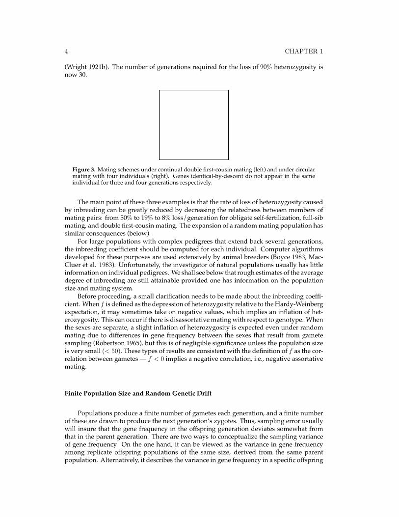
With a constant population size of four breeding adults, the minimum relationshipbetween individuals is that of double-first cousins (Figure 3). Starting with four unrelatedindividuals, it takes three generations for the appearance of alleles identical by descent inthe same individual, and thereafter

1− f(t) ' (0.92)t (1.3)

4 CHAPTER 1

(Wright 1921b). The number of generations required for the loss of 90% heterozygosity isnow 30.

Figure 3. Mating schemes under continual double first-cousin mating (left) and under circularmating with four individuals (right). Genes identical-by-descent do not appear in the sameindividual for three and four generations respectively.

The main point of these three examples is that the rate of loss of heterozygosity causedby inbreeding can be greatly reduced by decreasing the relatedness between members ofmating pairs: from 50% to 19% to 8% loss/generation for obligate self-fertilization, full-sibmating, and double first-cousin mating. The expansion of a random mating population hassimilar consequences (below).

For large populations with complex pedigrees that extend back several generations,the inbreeding coefficient should be computed for each individual. Computer algorithmsdeveloped for these purposes are used extensively by animal breeders (Boyce 1983, Mac-Cluer et al. 1983). Unfortunately, the investigator of natural populations usually has littleinformation on individual pedigrees. We shall see below that rough estimates of the averagedegree of inbreeding are still attainable provided one has information on the populationsize and mating system.

Before proceeding, a small clarification needs to be made about the inbreeding coeffi-cient. When f is defined as the depression of heterozygosity relative to the Hardy-Weinbergexpectation, it may sometimes take on negative values, which implies an inflation of het-erozygosity. This can occur if there is disassortative mating with respect to genotype. Whenthe sexes are separate, a slight inflation of heterozygosity is expected even under randommating due to differences in gene frequency between the sexes that result from gametesampling (Robertson 1965), but this is of negligible significance unless the population sizeis very small (< 50). These types of results are consistent with the definition of f as the cor-relation between gametes — f < 0 implies a negative correlation, i.e., negative assortativemating.

Finite Population Size and Random Genetic Drift

Populations produce a finite number of gametes each generation, and a finite numberof these are drawn to produce the next generation’s zygotes. Thus, sampling error usuallywill insure that the gene frequency in the offspring generation deviates somewhat fromthat in the parent generation. There are two ways to conceptualize the sampling varianceof gene frequency. On the one hand, it can be viewed as the variance in gene frequencyamong replicate offspring populations of the same size, derived from the same parentpopulation. Alternatively, it describes the variance in gene frequency in a specific offspring

INBREEDING AND GENETIC DRIFT 5

population among all loci with gene frequency p in the parental generation. The implicationof both viewpoints is the same. In the absence of any counteracting evolutionary forces, thedispersive effects of genetic drift will continue each generation until all loci have becomefixed for a single allele. The consequences of random drift are therefore two-fold: 1) thegenetic variation within populations is gradually lost as gene frequencies drift to zero orone, and 2) isolated populations diverge as they become fixed for alternate alleles.

To put things on a more formal basis, consider a large pool of gametes, a fraction p ofwhich contain the B allele. 2N gametes are randomly drawn to produce a new generationof size N . The expected frequencies of genotypes BB, Bb, and bb are, from the Hardy-Weinberg expectation, p2, 2p(1−p), and (1−p)2. The expected number of B alleles containedin any offspring is simply 2×p2+1×2p(1−p) = 2p, but the expected square of the number ofB alleles carried is 22×p2+12×2p(1−p) = 2p(1+p). The variance in the number of B allelescarried by each individual is therefore 2p(1 + p)− (2p)2 = 2p(1− p), while the variance forthe total number of B alleles carried by theN offspring is 2Np(1− p). Since 2N genes havebeen drawn, the variance of the frequency of allele B is 2Np(1− p)/(2N)2 = p(1− p)/2N .Thus, the sampling variance of gene frequency is directly proportional to the heterozygosityand the reciprocal of population size.

The expression p(1−p)/2N only defines the dispersion that results from a single gener-ation of gamete sampling, conditional on gene frequency p in the parent population. A fulleraccount of the long-term consequences of genetic drift requires an alternate approach. Thetheory will first be described for an idealized situation: 1) a monoecious, randomly matingpopulation that produces an effectively infinite number of gametes, 2) with non-overlappinggenerations, 3) a complete absence of evolutionary forces such as selection, migration, andmutation, and 4) constant population size. Later in the chapter, it will be shown how theidealized model can be generalized to incorporate different systems of mating.

Long-term loss of genetic variation within populations. Even when mating is completelyrandom, there is always a small chance that uniting gametes will derive from related indi-viduals. For example, in a randomly mating, monoecious population containing only twoindividuals, there are only four possible genes at each locus. Therefore, the probability thata gamete will randomly unite with another containing a direct copy of the same gene is1/4. With four individuals, there are eight genes, and this probability becomes 1/8. Thus,in the idealized situation, the probability that two direct copies of any parental gene willrandomly unite in an offspring is 1/2N .

Although the quantity 1/2N may be thought of as the new inbreeding that is incurredeach generation, this does not fully describe the build-up of homozygosity in a population.Even if uniting gametes do not carry genes that are direct copies of a parental gene, theymay still be identical-by-descent because of inbreeding in a previous generation. Underrandom mating, the probability of this event is simply the inbreeding coefficient of theparental generation. Thus, since the probability of drawing genes that are not direct copiesof the same parental gene is (1− 1/2N), the expected inbreeding coefficient in generation tis

f(t) =1

2N+

(1− 1

2N

)f(t− 1) (1.4)

Subtracting both sides from 1, this simplifies to the recursion formula

1− f(t) =

(1− 1

2N

)[1− f(t− 1)] (1.5a)

which generalizes to

1− f(t) =

(1− 1

2N

)t[1− f(0)] (1.5b)

6 CHAPTER 1

Note that as t → ∞, [1 − f(t)] → 0 at a rate that is inversely proportional to populationsize. Individuals are expected to become completely inbred at loci that are unmodified byselection, mutation, and migration.

It is important to bear in mind that the equations given above predict the expectedchanges in f resulting from inbreeding. Because of variation in pedigree structure, theactual degree of inbreeding generally will vary between loci within individuals as well asbetween individuals within the population. For any locus, identity by descent is binomi-ally distributed with mean f and variance σ2

f = f(1 − f). With completely linked loci,this is also the total variance in f since there is no variation in f between loci. However,for unlinked loci, the realized inbreeding at each locus need not be the same. The coeffi-cient of variation of (1 − f) is approximately (3N)−1/2 for randomly mating monoeciouspopulations, (6N)−1/2 for randomly mating but monogamous, dioecious populations, and(12N)−1/2 for monoecy with selfing excluded and for dioecy with random mating (Weir etal. 1980). These asymptotic values are reached in only a few generations. Thus, providedthe population size and number of constituent loci are moderately large, the variation ininbreeding is negligible for most practical purposes. Further information on this subjectmay be found in Jacquard (1975), Franklin (1977), and Cockerham and Weir (1983b).

Recall that [1 − f(t)] is the expected heterozygosity (Ht) relative to that in the basepopulation (H0).From Equation (1.5) we see that after tgenerations at a constant populationsize N ,

Ht =

(1− 1

2N

)tH0 (1.6)

where H0 is the initial heterozygosity. See Bulmer (1980; p. 220) for an expression for thevariance of Ht. This rate of decay of heterozygosity of 1/2N was first obtained by Wright(1931) using a rather different approach. It may be of interest to the non-mathematicallyinclined that Fisher, an excellent mathematician, obtained the wrong answer in 1922.

The time course for the loss of heterozygosity can be clarified by considering the ex-ponential approximation to Equation 1.6. Since (1 − x)t ' exp(−xt) for |x| << 1, forN > 10,

Ht ' H0 exp(−t/2N) (1.7)

This can be solved to show that the heterozygosity is reduced to half of H0 in about 1.4Ngenerations and to 5% of H0 in about 6N generations. If the population size is variable,Equation 1.6 becomes

Ht = H0

t∏i=1

(1− 1

2Ni

)(1.8)

where the∏

sign denotes a product of terms. This expression illustrates an importantpoint. Each of the terms, [1− (1/2Ni)], is necessarily less than one. Thus, an expansion ofpopulation size can only reduce the rate of erosion of heterozygosity; it cannot eliminate it.

Development of between-population variance. A natural consequence of gene frequencydrift within populations is the divergence of isolated replicate populations. Suppose a mo-noecious base population with gene frequency p0 is suddenly split into several completelyisolated subpopulations each of size N with random mating within each subpopulationand an absence of selection, migration, and mutation. The variance in gene frequency ingeneration t is

σ2p(t) = E(p2

t )− E2(pt)

INBREEDING AND GENETIC DRIFT 7

Adding and subtracting E(pt),

σ2p(t) = [E(pt)− E2(pt)] + [E(p2

t )− E(pt)]

= E(pt)[1− E(pt)]− E[pt(1− pt)]

Because there are no systematic forces causing the gene frequency to increase or decrease,E(pt) = p0, and the first quantity on the right is p0(1− p0). The quantityE[pt(1− pt)] is halfthe expected heterozygosity in a population in generation t. Substituting Equation (1.6),

σ2p(t) = p0(1− p0)

[1−

(1− 1

2N

)t](1.9a)

which is well approximated by

σ2p(t) ' p0(1− p0)[1− exp(−t/2N)] (1.9b)

for N > 10. Thus, the between-population variance asymptotically approaches p0(1− p0),which for a diallelic locus is half the heterozygosity in the base population. As the processof random drift proceeds, gene frequencies may go through many phases of increase anddecline, but eventually each gene will be totally fixed or lost. Ignoring new mutations, theprobability that an allele is ultimately fixed in a replicate population is its initial frequencyp0, while its probability of loss is (1− p0).

Equation 1.9 does not fully describe the pattern of development of differences betweenlines. For example, it yields little insight into the actual form of the distribution of populationgene frequencies, and it does not specify the probability of fixation of alleles. However,the idea that many allelic variants at enzymatic loci are selectively neutral (Kimura 1983)generated much interest in these issues, and the theory is now well developed.

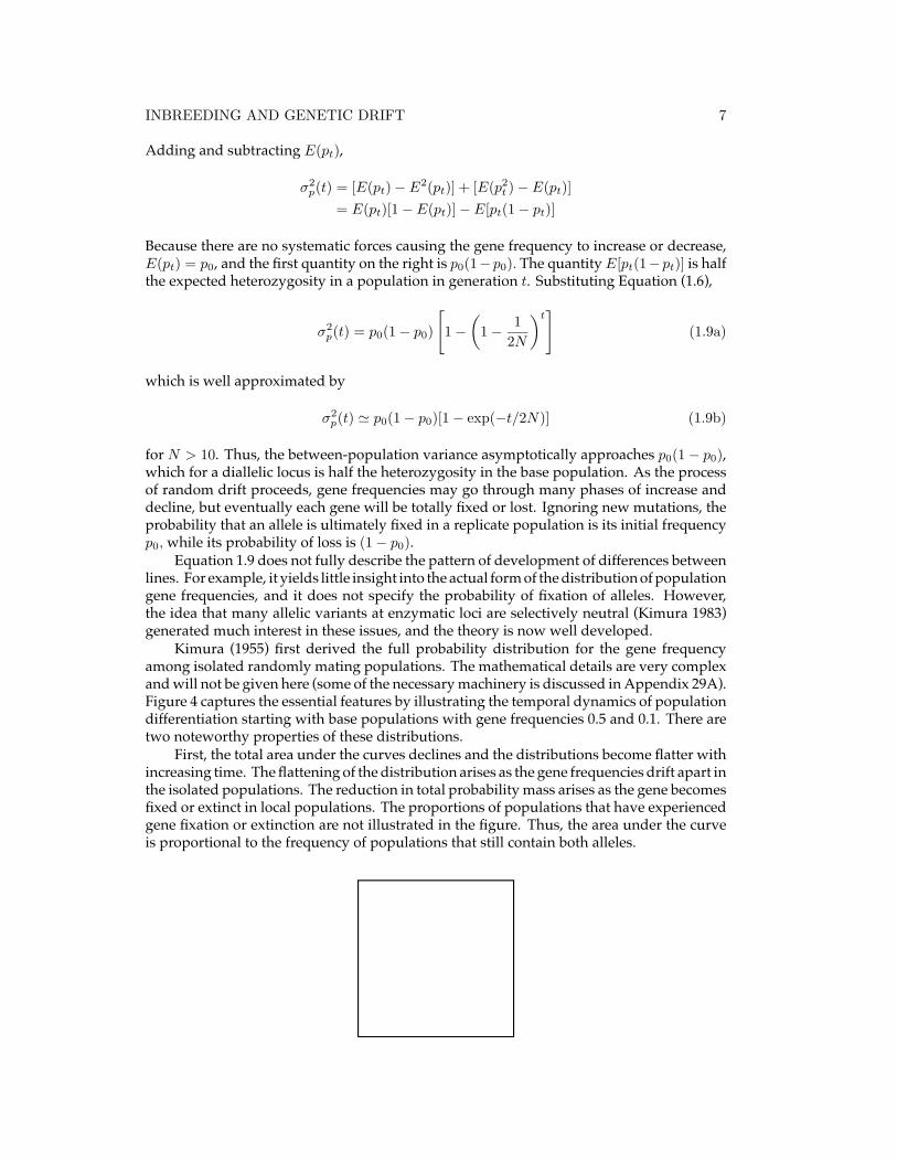
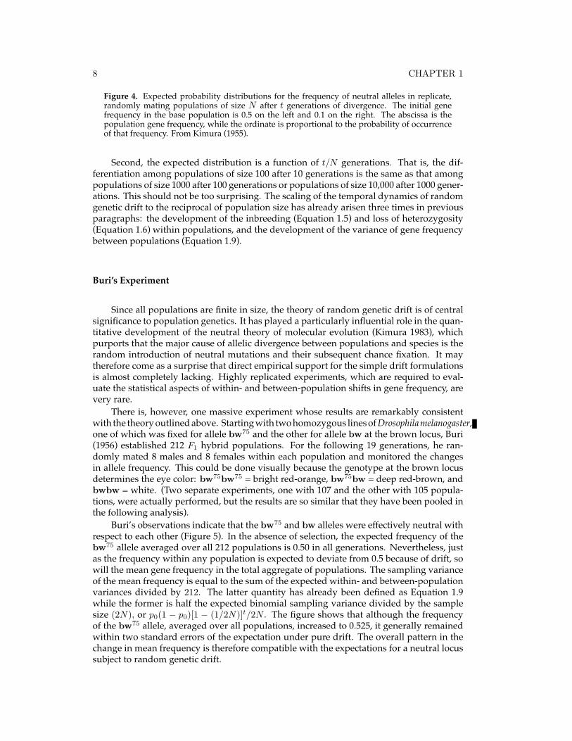
Kimura (1955) first derived the full probability distribution for the gene frequencyamong isolated randomly mating populations. The mathematical details are very complexand will not be given here (some of the necessary machinery is discussed in Appendix 29A).Figure 4 captures the essential features by illustrating the temporal dynamics of populationdifferentiation starting with base populations with gene frequencies 0.5 and 0.1. There aretwo noteworthy properties of these distributions.

First, the total area under the curves declines and the distributions become flatter withincreasing time. The flattening of the distribution arises as the gene frequencies drift apart inthe isolated populations. The reduction in total probability mass arises as the gene becomesfixed or extinct in local populations. The proportions of populations that have experiencedgene fixation or extinction are not illustrated in the figure. Thus, the area under the curveis proportional to the frequency of populations that still contain both alleles.

8 CHAPTER 1

Figure 4. Expected probability distributions for the frequency of neutral alleles in replicate,randomly mating populations of size N after t generations of divergence. The initial genefrequency in the base population is 0.5 on the left and 0.1 on the right. The abscissa is thepopulation gene frequency, while the ordinate is proportional to the probability of occurrenceof that frequency. From Kimura (1955).

Second, the expected distribution is a function of t/N generations. That is, the dif-ferentiation among populations of size 100 after 10 generations is the same as that amongpopulations of size 1000 after 100 generations or populations of size 10,000 after 1000 gener-ations. This should not be too surprising. The scaling of the temporal dynamics of randomgenetic drift to the reciprocal of population size has already arisen three times in previousparagraphs: the development of the inbreeding (Equation 1.5) and loss of heterozygosity(Equation 1.6) within populations, and the development of the variance of gene frequencybetween populations (Equation 1.9).

Buri’s Experiment

Since all populations are finite in size, the theory of random genetic drift is of centralsignificance to population genetics. It has played a particularly influential role in the quan-titative development of the neutral theory of molecular evolution (Kimura 1983), whichpurports that the major cause of allelic divergence between populations and species is therandom introduction of neutral mutations and their subsequent chance fixation. It maytherefore come as a surprise that direct empirical support for the simple drift formulationsis almost completely lacking. Highly replicated experiments, which are required to eval-uate the statistical aspects of within- and between-population shifts in gene frequency, arevery rare.

There is, however, one massive experiment whose results are remarkably consistentwith the theory outlined above. Starting with two homozygous lines of Drosophila melanogaster,one of which was fixed for allele bw75 and the other for allele bw at the brown locus, Buri(1956) established 212 F1 hybrid populations. For the following 19 generations, he ran-domly mated 8 males and 8 females within each population and monitored the changesin allele frequency. This could be done visually because the genotype at the brown locusdetermines the eye color: bw75bw75 = bright red-orange, bw75bw = deep red-brown, andbwbw = white. (Two separate experiments, one with 107 and the other with 105 popula-tions, were actually performed, but the results are so similar that they have been pooled inthe following analysis).

Buri’s observations indicate that the bw75 and bw alleles were effectively neutral withrespect to each other (Figure 5). In the absence of selection, the expected frequency of thebw75 allele averaged over all 212 populations is 0.50 in all generations. Nevertheless, justas the frequency within any population is expected to deviate from 0.5 because of drift, sowill the mean gene frequency in the total aggregate of populations. The sampling varianceof the mean frequency is equal to the sum of the expected within- and between-populationvariances divided by 212. The latter quantity has already been defined as Equation 1.9while the former is half the expected binomial sampling variance divided by the samplesize (2N), or p0(1 − p0)[1 − (1/2N)]t/2N . The figure shows that although the frequencyof the bw75 allele, averaged over all populations, increased to 0.525, it generally remainedwithin two standard errors of the expectation under pure drift. The overall pattern in thechange in mean frequency is therefore compatible with the expectations for a neutral locussubject to random genetic drift.

INBREEDING AND GENETIC DRIFT 9

Figure 5. Temporal change in the frequency of the bw75 allele, averaged over 212 isolatedpopulations of Drosophila melanogaster, each consisting of 8 breeding males and 8 breedingfemales. The dashed line denotes the expectation for a neutral allele plus two standard errors.From Buri (1956).

The dynamics of the between-population divergence (Figure 6) are qualitatively verysimilar to the expected pattern illustrated in the left panel of Figure 4. As the populationgene frequencies diverge, the initially bell-shaped distribution becomes flatter and thenbegins to acquire a U-shape as populations that are fixed for the bw75 or bw alleles beginto accumulate. Eventually, the distribution would have consisted of only two classes, thosefixed for bw75 and those fixed for bw, in roughly equal frequency.

Figure 6. Distribution of the number of bw75 genes in 212 populations of Drosophila melanogastereach initiated with a frequency of 0.5. From Buri (1956).

The actual rate of divergence illustrated in Figure 6 is somewhat greater than thatexpected for randomly mating populations of 16 individuals. However, this does not nec-essarily invalidate the theory outlined above. It is possible, for example, that not all 16potential parents reproduced each generation, and/or that the distribution of family sizesdeviated from randomness. From the standpoint of genetic drift, either of these conditionswould cause the populations to behave effectively as though they were smaller than theactual size.

With the massive amount of data in Buri’s experiment, it was possible to obtain anempirical estimate of this effective population size. Recall that the sampling variance ofgene frequency from one generation to the next is p(1− p)/2N . Not including fixed classes,there are 31 possible gene frequencies in Buri’s populations (1/32 to 31/32). Each of these31 classes was observed at various times in one or more of the 212 populations. Focusingon any one class, the sampling variance conditional on p could then be calculated from thegene frequencies observed in the subsequent generation. The 31 points shown in Figure 7provide an empirical description of the function p(1−p)/2N . An excellent fit is obtained if itis assumed that the average effective population size wasN = 10.2 rather than the idealized

10 CHAPTER 1

16. In other words, the sampling variance of gene frequency is in very close accord withthat expected for an average ideal population of 10.2 randomly mating individuals.

Figure 7. Observed sampling variances of gene frequency for situations in which the donorpopulation contained 1 to 31 bw75 genes. The dashed line is the expected pattern, p(1−p)/2N ,if the actual populations of 8 males and 8 females were randomly mating and all had an equalchance of contributing offspring. The solid line describes the pattern for an average effectivepopulation size of 10.2. From Buri (1956).

Figure 8 shows that when N is set equal to 10.2 in Equations 1.6 and 1.9, the ero-sion of average heterozygosity within populations and the build-up of between-populationvariance of gene frequency are quite consistent with the neutral model.

Figure 8. Reduction in the mean heterozygosity within populations and build-up of genefrequency variance between-populations for the brown locus in 212 replicate populations ofDrosophila melanogaster. Fitted lines are Equations 1.6 and 1.9 with p0 = 0.5 andN = 10.2. Theexpected heterozygosity is 0.5 in generations 1 and 2 because the base population (generation 0)consisted entirely of heterozygotes, and because with separate sexes, an additional generationis required for the unification of alleles that are identical by descent. From Buri (1956).

Avoidance of the Loss of Genetic Variation

The genetic consequences of inbreeding and random genetic drift are of particularconcern to managers of small, captive populations of endangered species. Here we considerjust one of the many practical questions that arise in this area. Given a limited number offounders and an upper ceiling on the number of individuals that can be maintained, whatis the optimal breeding scheme for minimizing the erosion of genetic variance? In his 1921bpaper, Wright suggested that the best way to minimize the build-up of homozygosity in a

INBREEDING AND GENETIC DRIFT 11

small population would be to restrict matings to pairs of individuals with the least degreeof relatedness. Such a breeding scheme is known as maximum avoidance of inbreeding orMAI and is exemplified by the double first-cousin mating design in Figure 3. An addedadvantage of MAI is that for a population size of N = 2m, m generations pass before anyinbreeding occurs at all. For example, with N = 64 under a maximum avoidance scheme,m+1 = 7 generations would pass before two copies of a founding gene could appear in thesame individual. Once the inbreeding begins, the proportion of heterozygosity lost eachgeneration is very nearly constant, as pointed out above for population sizes of 1, 2, and 4.More generally, forN ≥ 4, the erosion of heterozygosity under MAI is closely approximatedby

1− f(t) '(

1− 1

4N

)t(1.10)

where t is the number of generations after the onset of inbreeding (Wright 1951). Comparingthis expression with Equation (1.5), it can be seen that MAI has the same effect as doublingthe size of a random mating population.

Kimura and Crow (1963a) subsequently noted that Wright’s intuition that MAI mini-mizes the long-term loss of genetic variation is not strictly correct. A circular mating (CM)scheme (Figure 3) leads ultimately to a lower rate of loss of heterozygosity. Under thisbreeding design, females and males are arranged such that each of them is mated to two“neighbors.” The last individual in the linear array is mated with the first, thereby complet-ing the circle. Although circular mating ultimately reduces the rate of loss of heterozygosityrelative to MAI, it is inferior in the early generations of mating, and even with small N , itmay take 100 or more generations before its superiority is realized. Since most of the geneticvariation has been lost by this time, the practical utility of circular mating is questionable.

The major limitation of both the MAI and CM schemes is that they only impede theloss of genetic variation. Ignoring new mutations, any randomly mating finite populationwill ultimately become homozygous at every locus. Robertson (1964) obtained the moregeneral (and counterintuitive) result that the rate of loss of overall genetic variation actuallydeclines as the relatedness between mates increases. In the extreme, genetic diversity canbe preserved indefinitely by subdividing a population into several isolated lines. Althoughthe individual lines are all expected to become homozygous eventually, different lines arelikely to become fixed for different sets of genes. Subsequent crossing of the lines wouldthen restore the population to something close to its original state. It must be emphasized,however, that the preceding arguments assume that intense inbreeding in small lines hasno serious selective consequences that might endanger the survival of the lines. In reality,very small lines are likely to die out occasionally just by accident, and extreme inbreedingoften has serious deleterious effects on fitness (Chapter 22). Many of the technical detailson the dynamics of inbreeding and random genetic drift in subdivided populations can befound in Cockerham (1970).

Effective Population Size

Up to now, we have assumed a randomly mating population, constant in size, andconsisting of a homogeneous set of monoecious, self-compatible individuals. Since almostall populations deviate from this ideal structure in some way, the question arises as to therelevance of the preceding theory. In fact, much of the theory of inbreeding and randomgenetic drift can be generalized to other types of population structure in a relatively simplemanner. Instead of relying on the total number of individuals as a measure of population

12 CHAPTER 1

size, we construct a surrogate index that takes into account the deviations from the idealmodel. Such an index has become widely known asNe, the effective population size, followingthe early and influential work of Wright (1931, 1938, 1939).

In an ideal monoecious population, each gamete unites randomly with another gametederived from the total population ofN individuals. Thus, the probability that two randomlyuniting gametes are derived from the same parent is simply P = 1/N . Many factorsincluding self-incompatibility, limited dispersal, differential productivity of gametes, andselection can causeP to deviate from the reciprocal of the actual population size. To accountfor this, P can be more generally regarded as the reciprocal of the effective rather than theactual population size.

To see the connection betweenNe and the inbreeding in a population more clearly, recallthe approach to predicting the future inbreeding coefficient in a population. The probabilitythat two uniting gametes are derived from the same parent is now 1/Ne in which case thereis a 50% chance that they each carry copies of the same gene (identical by descent) and a50% chance that they carry copies of different genes. In the latter case, the uniting genesmay still be identical by descent with probability f(t−1) from previous inbreeding. Finally,there is a 1− (1/Ne) probability that the uniting gametes are derived from different parents,in which case there is again a probability f(t − 1) that they are identical by descent fromprevious inbreeding. Summing up the three ways in which identity-by-descent can arisebetween uniting gametes,

f(t) =

(1

Ne

)(1

2

)+

(1

Ne

)(1

2

)f(t− 1) +

(1− 1

Ne

)f(t− 1)

=1

2Ne+

(1− 1

2Ne

)f(t− 1) (1.11)

Notice that this expression is identical in form to Equation 1.4. Thus, the effective populationsize may be viewed as the size of an ideal population that would exhibit the same amountof inbreeding as the population under consideration. For reasons to be discussed below,the effective population size is almost always less than the actual size.

The effective population size is one of the most important parameters in populationgenetics. It enters almost all expressions for the dynamics and equilibrium states of genefrequencies in finite populations. WhileNe is not as easily measured in natural populationsas the total population size, it is at least in principle obtainable from observable demographicproperties of populations (Latter 1959, Lande and Barrowclough 1987, Crow and Denniston1988), as we now demonstrate.

Monoecy. In order to illustrate the mathematical approach to derive expressions for Ne,we first generalize the monoecious, self-compatible population to allow arbitrary numbersof gametes to be contributed by different members of the population. Let ki be the numberof gametes that the ith parent contributes to offspring that survive to maturity. µk andσ2k are the mean and variance of successful gamete production per individual, and Nt−1

is the number of reproducing parents. Assuming that mating is random and isogamous(no distinction between male and female gametes), there are ki(ki − 1) ways in which thegametes of parent i can unite with each other. Hence there are

∑Nt−1

i=1 ki(ki−1) total ways inwhich gametes can come from the same parent. In total, Nt−1µk gametes are produced, sothe probability that zygotes in generation t contain gametes derived from the same parentis

Pt =1

Ne=

∑Nt−1

i=1 ki(ki − 1)

Nt−1µk(Nt−1µk − 1)(1.12)

INBREEDING AND GENETIC DRIFT 13

This expression can be simplified greatly by noting that∑Nt−1

i=1 ki(ki − 1)/Nt−1 = E(k2)−µk = σ2

k+µk(µk−1) and thatNt−1µk = 2Nt. Substituting into Equation 1.12 and inverting,

Ne =2Nt − 1

(σ2k/µk) + µk − 1

(1.13)

Thus, for a randomly mating monoecious population with discrete generations, the effectivepopulation size is a function of the actual population size and the mean and variance ofsuccessful gamete production. In principle, all three quantities can be estimated in naturalpopulations.

The above expression simplifies greatly under a number of conditions. For example,for populations that are stable in size (µk = 2),

Ne =4Nt − 2

σ2k + 2

(1.14)

Consider also the situation in which each parent produces the same number of potentialgametes. Since the variance in the number of gametes of a particular parent for each gametedrawn is (1/Nt−1)[1− (1/Nt−1)] (from the properties of a binomial distribution), and sincea total of µkNt−1 gametes are drawn, σ2

k = µk[1 − (1/Nt−1)]. Substituting into Equation1.14, it is found that Ne = Nt−1. This is to be expected since the conditions assumed areidentical to those of the idealized model.

Many hermaphroditic species are self-incompatible in which case identity-by-descentfor pairs of uniting gametes comes through grandparents rather than parents. If we nowlet ki be the number of successful gametes for individual i in generation t − 2, there are2ki(ki − 1) ways in which pairs of genes from i can unite through matings in generationt− 1 (the 2 since each individual can serve as a mother or father). Since there are Nt−2µk/2parents in generation t−1, there are 2(Nt−2µk/2)[(Nt−2µk/2)−1] ways of drawing differentparents, and 4 · 2(Nt−2µk/2)[(Nt−2µk/2)− 1] ways of drawing gene pairs (the 4 since eachparent carries two genes). Therefore, the probability of drawing a pair of genes from thesame grandparent is

Pt =

∑Nt−2

i=1 ki(ki − 1)

Nt−2µk(Nt−2µk − 2)(1.15)

assuming that the fertility of parents and offspring are uncorrelated. Employing the samesubstitutions used for Equation 1.13,

Ne =2(Nt−1 − 1)

(σ2k/µk) + µk − 1

(1.16)

Note that for populations that are moderately large and stable in size, Equations 1.13 and1.16 give essentially the same answer — the prohibition of selfing has a negligible influenceonNe.The reason for this is that under random mating the increment in inbreeding resultingfrom self-fertilization is a transient event that can be completely undone in the followinggeneration.

In many hermaphroditic species, there is a distinction between male and female ga-metes (anisogamy). When mating is random but selfing is prohibited, the effective popula-tion size is the same under isogamy and anisogamy, i.e., Equation 1.16 still applies (Crowand Denniston 1988). However, with selfing permitted,

Ne =Nt−1

(4σep/µ2k) + 1

(1.17)

14 CHAPTER 1

whereσep is the covariance of the numbers of successful male and female gametes per parent(Crow and Denniston 1988). If σep is positive, as might be expected in a spatially heteroge-neous environment where some individuals acquire many more resources than others, theeffective population size will be less than the observed size provided the population size isstable (µk = 2). If σep is negative, as might be expected when there is a tradeoff betweenmale and female function, Ne can exceed Nt−1. This results because a negative covariancein male and female gamete production reduces the variance in family size.

All of the preceding examples indicate that variance in successful gamete productionis a major determinant of the effective population size. An increase in the variance offamily size causes a reduction in Ne because of the enhanced likelihood of uniting gametescoming from the same prolific parent in subsequent generations. When the variance infamily size is entirely a function of the random sampling of gametes (so that σ2

k = µk) andthe population size is stable (µk = 2), the effective population size is essentially equivalentto the number of reproductive adults. It may be more surprising that in the opposite andextreme situation in which all parents produce an identical number of progeny (σ2

k = 0),Ne = 2Nt−1−1 ' 2Nt−1, i.e., elimination of the variance in family size doubles the effectivepopulation size. It was shown earlier that the MAI scheme of mating results in a rate ofloss of heterozygosity of about 1/4N . This can now be seen to be a consequence of the MAImating scheme causing every parent to produce the same number of offspring.

In natural populations where individuals grow up in different microenvironments,which influence the availability of resources and mates, σ2

k will usually exceed the mean.Thus, generally we can expect the effective population size to be less than the number ofreproductive adults.

Example 1. Heywood (1986) has estimatedσ2k/µ

2k for seed production to be on the order of 1 to 4

in a number of annual plants. Unfortunately, the value ofσ2k for total gamete production requires

additional information on successful pollen production. Such information is extremely difficultto acquire due to problems in ascertaining paternity. For heuristic purposes, however, let usassume a stable monoecious population (µk for seed production = µk for pollen production= 1), a three-fold higher standard deviation for successful pollen production, and a perfectcorrelation between seed and pollen production, i.e., 1 = σep/[σk(seed) ·3σk(seed)]. Assuminga stable population size, what is Ne? Substituting σep = 3σ2

k(seed) and µk = 2 into Equation

1.17, Ne = N/(3σ2k(seed) + 1). For the cases in which σ2

k(seed) = 1 and 4, Ne is 25% and 8%of the census number.

tDioecy. As in the case of monoecy with self-incompatibility, when the sexes are separate,the new inbreeding needs to be defined with reference to the grandparents since this is theearliest generation back to which the two genes of an individual can be traced to the sameancestor. An additional complication that arises with separate sexes is the possibility thatthe inbreeding through males and females may differ. This is expected, for example, inpolygynous species in which most females mate with a relatively small segment of the malepopulation. It is also expected in species with skewed sex ratios.

If O is the individual of interest and X and Y its mother and father, then there are twoways in whichO may derive two genes from the same grandparent: 1)X and Y may sharethe same mother (probability 1/Nef where 1/Nef is the effective number of females), or 2)X and Y may share the same father (probability 1/Nem). In each case, the probability that

INBREEDING AND GENETIC DRIFT 15

O inherits both genes from the shared grandparent is 1/4. Thus, the total probability thatO inherits two genes from the same grandparent is

P =1

Ne=

1

4Nem+

1

4Nef(1.18)

Assuming random mating (no prohibition of mating between sibs), the effective num-ber of each sex can be derived by the same method used to acquire Equation 1.13,

Nes =2Ns,t−1 − 1

(σ2sk/µsk) + µsk − 1

(1.19)

where s denotes the sex (m or f ) and µsk and σ2sk are the mean and variance of gamete

production by sex s. Latter (1959) provides a more elaborate expression for Nes that ex-plicitly accounts for the variance and covariance of male and female progeny production.Letting φ be the sex ratio (proportion of females), then the mean and variance of gameteproduction for the whole population are respectively µk = 2(1 − φ)µmk = 2φµfk andσ2k = (1 − φ)σ2

mk + φσ2fk + φ(1 − φ)(µmk − µfk)2, and Equation 1.18 yields Equation 1.16.

Thus, the effective size of an ideal population with separate sexes is the same as that for amonoecious, self-incompatible population with the same population properties µk and σ2

k.In a recent summary of data on lifetime reproductive success in birds, Grant (1990)

found that σ2fk/µfk ranged from 1.2 to 4.2, which is much greater than the ratio of 1 expected

under random mating. Assuming a stable population size (µfk = 2) and substituting intoEquation 1.19, the effective female population size for these species is found to be 40-90%of the actual number of females.

Further simplification of Equation 1.19 is possible when certain assumptions are met.Consider, for example, the case in which members of the same sex produce equal numbersof gametes so that the variation in family size is a simple consequence of the random unionof gametes. It then follows from the development of the monoecy model thatNem = Nm,t−1

and Nef = Nf,t−1. Rearranging Equation 1.18,

Ne =4Nm,t−1Nf,t−1

Nm,t−1 +Nf,t−1= 4φ(1− φ)Nt−1 (1.20)

Ne attains a maximum of Nt−1 when the sex ratio is balanced (φ = 0.5). With skewed sexratios, the effective size of the population is influenced much more strongly by the densityof the rarer sex than of the more abundant sex. For example, in a highly polygynous speciesas φ→ 1, Ne → 4(1− φ)Nt−1 ' 4Nm,t−1.

Age structure. The previous formulae have been obtained under the assumption of discretegenerations. Such expressions are reasonable for organisms such as annual plants (ignoringthe problem of seed banks) or univoltine insects, but for species that reproduce at differentages, as in the case of most vertebrates, generations overlap in time. It turns out that thisdoes not complicate things too much. The work of Hill (1972a, 1979) indicates a simplecorrespondence between the effective sizes of populations with and without age-structure.

In the previous formulations N was the number of reproductive individuals in thepopulation in each generation. For age-structured populations, it is convenient to con-sider Nb, the number of births during each unit of time multiplied by the number of timeunits/generation. The latter quantity, known as the generation time (T ), is the average ageof parents giving birth. For an ideal monoecious population,

T =

∑τi=1 ilibi∑τi=1 libi

(1.21)

16 CHAPTER 1

where li is the probability of surviving to age i and bi is the expected number of offspringproduced by parents of age i, and τ is the maximum reproductive age. For a dioeciouspopulation, T is complicated by the need to average over mothers and fathers,

T =Tmm + Tmf + Tfm + Tff

4(1.22)

where Tmf , for example, is the average age of male parents of daughters. LettingN = NbT,all of the preceding formulae apply provided the structure and size of the population arestable. We are still left, however, with the problem of estimating σ2

k, which now dependson variation in longevity as well as variation in fertility.

Felsenstein (1971), Johnson (1977a), and Emigh and Pollak (1979) have explicitly evalu-ated the variance in offspring production in terms of the age-specific schedules for survivaland reproduction. The assumption is again made that the population is stable in size, sexratio, and age composition. Letting φb be the sex ratio of newborns andNeb = 4φb(1−φb)Nbbe the “effective size” of the newborn age class, then the effective size of an age-structuredpopulation with separate sexes is

Ne =NebT

1 + (1− φb)∑τfi=1

(1

lfi+1

− 1

lfi

)∑2f +φb

∑τmi=1

(1

lmi+1

− 1

lmi

)∑2m

(1.23)

where the superscripts f and m denote the life-table parameters for females and males

and∑2s =

(∑τsj≥i+1 l

sjbsj

)2

(Emigh and Pollak 1979). An analogous expression is availablefor monoecious populations (Felsenstein 1971). While the derivations underlying theseexpressions rely on the assumption that gametes are drawn randomly from the memberswithin age classes, no assumptions are made with regard to the preference of matingsbetween age classes.

Despite their complicated structure, demographic formulae such as 1.23 are usefulfor the analysis of the sensitivity of a population’s effective size to modifications in thelife-history schedule that might result from ecological changes. Nevertheless, the Emigh-Pollak equation has some practical difficulties. First, it rests on the assumption of a stablepopulation structure. Such situations are rare in nature because of temporal changes inthe environment. Johnson (1977a) and Choy and Weir (1978) have derived dynamicalequations for inbreeding in age-structured populations in order to resolve these difficulties.The entire subject is reviewed by Charlesworth (1980). Second, Equation 1.23 has beenderived under the assumption that the age-specific mortality and birth rates of individualsare uncorrelated. This will not be true for populations in which energetic tradeoffs existbetween different life-history characters. The problem needs further investigation.

Table 1. The elements of the formula for the effective size of an age-structured population, Equation1.23, using the red deer as an example. While the age-specific survival rates, li, are extracted directlyfrom Clutton-Brock et al. (1982), the estimates of bfi and bmi are estimated from behavioral and de-mographic observations of the authors and are adjusted downward to maintain a stable populationsize. Columns marked (1) and (2) are [(1/lsi+1)− (1/lsi )] and (

∑τsj>i+1 l

sjbsj)

2, and column (3) is theproduct of (1) and (2).

Age Females Males

i lfi bfi (1) (2) (3) lmi bmi (1) (2) (3)

INBREEDING AND GENETIC DRIFT 17

1 1.00 0.00 0.33 0.25 0.08 1.00 0.00 0.45 5.97 2.692 0.75 0.00 0.12 0.25 0.03 0.69 0.00 0.22 5.97 1.313 0.69 0.00 0.02 0.25 0.01 0.60 0.00 0.03 5.97 0.184 0.68 0.18 0.04 0.24 0.01 0.59 0.00 0.03 5.97 0.185 0.66 0.26 0.07 0.22 0.02 0.58 0.00 0.03 5.97 0.186 0.63 0.33 0.05 0.21 0.01 0.57 0.34 0.03 5.92 0.187 0.61 0.34 0.06 0.19 0.01 0.56 0.26 0.03 5.88 0.188 0.59 0.40 0.06 0.17 0.01 0.55 0.60 0.10 5.59 0.569 0.57 0.42 0.03 0.16 0.01 0.52 0.53 0.12 5.30 0.6410 0.56 0.34 0.07 0.14 0.01 0.49 0.79 0.40 3.94 1.5811 0.54 0.46 0.03 0.13 0.00 0.41 0.53 0.42 3.11 1.3112 0.53 0.42 0.20 0.08 0.02 0.35 0.45 1.69 1.00 1.6913 0.48 0.45 0.19 0.04 0.01 0.22 0.08 2.60 0.63 1.6414 0.44 0.40 0.23 0.01 0.00 0.14 0.20 3.97 — —15 0.40 0.25 0.20 — — 0.09 — — — —16 0.37 0.00 — — — 0.05 — — — —

0.23 12.32

These problems aside, there are few age-structured populations that have been charac-terized well enough to implement the Emigh-Pollak equation. While complete age-specificsurvivorship and reproductive schedules are available for the females of many naturalpopulations, there are enormous practical difficulties in ascertaining paternity. Thus, thevariance in male reproductive success is generally unknown. A long-term study on thebehavior and demography of the red deer (Cervus elaphus) by Clutton-Brock et al. (1982)allows at least a crude estimate ofNe (Table 1). The study population was roughly constantin density for two decades, and observations on known individuals provide informationon the age-specific rates of mortality and reproduction for both sexes. The sex ratio at birth,φb, averaged 0.43 over several years, so Neb = 0.98Nb.

The summations in the denominator of Equation 1.23 reflect the variation in lifetimereproductive success of females and males respectively. For the red deer, these terms areequal to 0.23 and 12.32, indicating a great inequity between the reproductive properties ofthe sexes. This is to be expected since males appropriate harems, and older males are muchmore successful at it than young ones. The few males that live to an old age may father upto two dozen offspring in their lifetime, whereas the large fraction of males that die beforethe age of 5 (∼ 40%) has no reproductive success at all. On the other hand, since malesinseminate multiple females, almost all females reproduce to some degree once they haveattained reproductive maturity.

Substituting the sums in Table 1 into Equation 1.23, the effective population size isfound to be 0.98NbT/[1 + (1 − 0.43)(0.23) + 0.43(12.32)] = 0.15NbT . Thus, the effectivesize of this population is on the order of 15% of the number of offspring produced by thepopulation/generation. The mean generation time through females and males is 9.47 and9.18 years, so T ' 9.32. The annual number of offspring produced by the population isapproximately 270 (S.D. = 40). Thus, Ne ' 0.15× 270× 9.32 = 378.

For comparative purposes, it is sometimes useful to convert the effective size of anage-structured population to an annual effective size, Ny = TNe, which is the size of anideal monoecious population with a generation time of one year that corresponds to theannual increment in inbreeding in the observed population. For the red deer example,Ny = 9.32× 378 = 3523.

18 CHAPTER 1

Variable population size. Most populations vary in density from generation to gener-ation, often dramatically so, and this raises practical problems in the implementation ofthe previous theory. The expected loss of heterozygosity over t generations is no longer[1 − (1/2Ne)]

t but a product of t terms, each incorporating the effective population size ofa particular generation,

Ht = H0

t−1∏i=0

(1− 1

2Nei

)(1.24)

It is sometimes of interest to evaluate the size of an ideal population that would have thesame expected heterozygosity after tgenerations of inbreeding as a population with variablesize over the same period. An approximate answer can be obtained by noting that withmoderately large Nei, Equation 1.24 simplifies to

Ht ' H0 exp

(−t−1∑i=0

1

2Nei

)(1.25)

which may be compared toHt ' H0 exp(−t/2Ne)

for the ideal case of constant effective size. Equating the exponents of these two expressions

N∗e 't

1

Ne0+

1

Ne1+ · · ·+ 1

Ne,t−1

(1.26)

The long-term effective sizeN∗e is approximately equal to the harmonic mean of the generation-specific effective sizes. A star is placed on Ne to remind the reader that the inbreedingprojected by N∗e strictly pertains to generation t. Other generations may exhibit more orless loss of variation than anticipated by projection of exp(−t/2N∗e ) depending upon thetemporal changes in Nei.

Example 2. Population bottlenecks have especially pronounced effects on N∗e . To see this,consider a population whose effective size regularly fluctuates between 10 and 100. FromEquation 1.26, N∗e = 2/(0.1 + 0.01) = 18.2. Thus, the total loss of heterozygosity from thispopulation every two generations is equivalent to that expected for an ideal random matingpopulation with a constant effective size of 18. This is much closer to the expectation for aconstant population size of 10 than 100.

Some work has been done on the effective size of populations consisting of patchessubject to periodic extinctions and recolonizations (Maruyama and Kimura 1980, Ewens etal. 1987, Ewens 1989a). Although it is highly technical, this work is of great relevance tonatural populations. There is room for much further study here, since the current modelsmake some rather unlikely assumptions about patterns of colonization.

Partial inbreeding. In all of the previous formulations, the assumption has been made thatthe union of gametes is random. More realistically, we might expect the frequency of matingbetween relatives to exceed that expected under random mating. Many plants, for example,

INBREEDING AND GENETIC DRIFT 19

produce a high proportion of their offspring by self-fertilization. If the total population sizeis infinite, a fixed proportion of matings between relatives leads to an equilibrium at whichthe production of new inbreeding each generation is balanced by the breakdown of oldinbreeding through outcrossing (Wright 1951, 1969, Hedrick 1986, Hedrick and Cockerham1986). Such an equilibrium does not exist for finite populations since the gene frequency issubject to random genetic drift.

Wright (1951) gave limited attention to this matter, and there has been little work on thesubject since then. Pollak (1987) has recently developed a general theory for partial selfing,showing that

Ne =4Nt

(1− β

2

)− 2(

1 + β2−β

)[σ2k + 2(1− β)]

(1.27)

where β is the frequency of selfing. If the population size is moderately large and stable,gamete production is uniform among individuals, and outcrossed matings random, thissimplifies to

Ne '(2− β)Nt

2(1.28)

Partial selfing introduces further complications into the theory of inbreeding. The standardequation for the erosion of average heterozygosity (1.5) is replaced by

1− f(t) '[(

1− β

2− β

)(1− 1

2Ne

)t+

β

2− β

(β

2

)t][1− f(0)] (1.29)

(Pollak 1987). This is another area in which there is room for much more work.

Additional Considerations

Earlier in the chapter, it was emphasized that the effects of finite population size aretwofold: the development of homozygosity within populations and the divergence of genefrequencies between replicate populations. Crow (1954) has emphasized that the formeris most closely related to the number of parents (or grandparents) since it is based uponthe probability of uniting gametes coming from the same ancestor. On the other hand,random gene frequency drift is primarily a function of the number of offspring producedsince it is based on sampling error in the gamete stage. Thus, in an expanding or decliningpopulation, the rates of inbreeding and gene frequency drift depend on different populationsizes. In order to clarify this distinction, Crow (1954) defined an inbreeding effective size(N I

e ) and a variance effective size (NVe ).

In all of the previous applications of the concept of effective population size, we wereconcerned with N I

e . The variance effective size is defined to be the size of an ideal mo-noecious population that yields the binomial sampling variance of the gene frequency,p(1 − p)/2NV

e , which matches that observed in a set of non-ideal replicate populations.General formulae for the variance effective size are available in Kimura and Crow (1963b),Crow and Kimura (1970), Crow and Morton (1955), and Crow and Denniston (1988).

The purpose of the preceding sections was to illustrate how the effective populationsize can be estimated if one can quantify the total size and various attributes of the matingsystem of the population. Under many circumstances, however, it is not possible to obtainall of the necessary demographic data. An alternative approach is the indirect methodof monitoring temporal changes in gene frequencies, usually with allozyme markers, and

20 CHAPTER 1

inferring the effective population size that is necessary to account for such change underthe assumption that the markers are selectively neutral (Pollak 1983, Tajima and Nei 1984,Waples 1989, Weir 1990).

It should now be amply clear that the loss of heterozygosity from populations canresult from two causes. The first of these, inbreeding due to consanguineous mating, is ina sense transient because it can be eliminated completely with one generation of randommating. The loss of heterozygosity resulting from finite population size is more permanentunless several isolated populations are available for crossing. Up to now, we have treatedthese two components of random genetic drift separately, but both can, and usually do,occur simultaneously in natural populations. Moreover, the effects of finite population sizecan often operate on several levels. Species are generally subdivided into several partiallyor completely isolated populations, which in turn may be fragmented into local demes,which may be further structured into family groups. Clearly, if one wants to characterizethe mechanisms of random genetic drift in natural populations, a means for partitioningthe causal sources is required.

Wright (1951, 1965, 1973) developed an ingenious framework for attacking the problem.The strategy is to take a hierarchical view of population structure. Consider the simplesituation in which the total population is divided into several isolated subpopulationswithin which there may be nonrandom mating. Letting fIT be the average inbreedingcoefficient for members of the entire population, then (1 − fIT ) is the probability that arandomly chosen individual is not inbred at a particular locus. This must be equal to theproduct of the probability of not being inbred because of residence in a subpopulation offinite size (1 − fST ) and the probability of not being inbred because of consanguineousmating within the subpopulation (1−fIS).Wright’s f−statistics can be interpreted directlyin terms of the observed and expected levels of heterozygosity at the total population andsubpopulation levels. Consequently, several estimation procedures, which rely on observedmeasures of allozyme or nucleotide variation, are available (Nei 1987, Weir 1990).