This paper is forthcoming in Industrial and Labor Relations Review.

In Search of the Glass Ceiling:

Gender and Earnings Growth among U.S. College Graduates in the 1990s

Catherine Weinberger University of California Santa Barbara

weinberg@isber.ucsb.edu

First Draft: May 2005 This version: December 2010

Gender-typical educational choices and lower rates of earnings growth, or the "glass ceiling," are widely believed to explain why older women earn far less than observably similar men. Using panels of college-educated workers from the 1990s, I search for differential growth rates predicted by both human capital and discrimination models. To the contrary, this study finds similar average rates of earnings growth for women and men across numerous specifications, suggesting that the gender gap in earnings is determined by factors already present early in the career; however, changes in educational choices explain only a tiny fraction of between-cohort narrowing of the gender gap. Further exploration reveals slower earnings growth by women within two groups: The first is young mothers, who experience slower earnings growth during the early career relative to men the same age, but then more than compensate with faster growth later in their careers. The second is the group of women with exceptionally high earnings levels; relative to men the same age with similarly high levels of attainment, women are underrepresented among workers winning the largest promotions. This phenomenon affects a very small, but potentially influential, subset of women facing a glass ceiling at the very top of the career ladder. This material is based upon work supported by the National Science Foundation under Grant No. 0120111. The use of NSF data does not imply NSF endorsement of the research methods or conclusions contained in this report. Any opinions, findings, and conclusions or recommendations expressed in this material are those of the author and do not necessarily reflect the views of the National Science Foundation. I thank Peter Kuhn for many helpful conversations, and Sarah Andresen for excellent research assistance. Patricia Anderson, Donna Ginther, Sarah Turner and anonymous referees also offered insightful suggestions.

2

Introduction

The highly visible CONSAD report on the status of women in the U.S. labor force attributes

the majority of the current gender earnings gap to women’s choices, including gender-typical

educational choices and the allocation of time between career development and family care

(2009). However, the research on which the CONSAD report is based relies primarily on data

with severe limitations for observing the dynamic processes leading to adult earnings outcomes.

The research presented here utilizes a unique longitudinal survey of highly-educated men and

women of all ages, followed for 4-10 years, to carefully document the small role played by both

pre-labor-market educational choices and contemporaneous family responsibilities in the

between-cohort narrowing of the gender earnings gap among U.S. college graduates.

This paper combines information from several sources, including the nationally

representative NSF National Survey of College Graduates (with a short panel of annual earnings

data from 1989 and 1993) and four panels drawn from the NSF SESTAT Surveys of scientists

and engineers (with annual earnings from 1989-1999, or hourly earnings from 1989-1996). The

shortest panel is representative of U.S. college graduates as of the 1990 Census, and includes

detailed information on income, college major and higher degrees for more than 40,000

individuals. The longer panels are selected subsets of the shorter, with the advantage of detailed

data on contemporaneous family formation and labor force participation. In these panels

earnings growth is measured over a ten-year interval for nearly 2000 women and 9000 men, or

over a seven-year interval for more than 4000 women and 13000 men.

Previous research based on data from the National Survey of College Graduates utilizes the

detailed information available in the base year cross-section to estimate the proportion of the

gender wage gap due to usually unobserved dimensions of human capital, particularly the choice

of college major (Black et. al. 2008). However, the true impact of a retrospective measure of

labor force experience is impossible to estimate in cross-section data. In a final footnote, Black

et. al. (2008) note that: “…it is possible that women who have high labor force attachment are

disproportionately among the most talented women (along dimensions that are not measured in

our data), and we may be therefore underestimating wage gaps for women generally when we

focus on this group.” In other words, it is possible that labor force attachment and current

earnings potential are jointly determined by factors that were already present when an individual

entered the labor force—including both individual characteristics, and features of the labor

3

market at the time. Improved understanding of the evolution of gender wage gaps requires panel

data that follows individuals over time, allowing comparison of a given cohort’s gender wage

gap at the outset and the conclusion of the time interval, and evaluation of the relationship

between each individual’s earnings growth path and contemporaneous events.

It is abundantly clear from earlier research that women are less likely than men to choose the

most remunerative technical college majors, and that this pattern has been quite persistent (Blau

and Ferber 1986, Eide 1994, Brown and Corcoran 1997, Weinberger 1998, 1999, 2001, Carrell,

Page and West 2010). In all previous cross-section studies, gender differences in college major

choices explain a substantial portion of the gender gap in earnings among college graduates

(Blau and Ferber 1986, Brown and Corcoran 1997, Weinberger 1998, 1999, 2001, Black et. al.

2008). However, little of the narrowing of the gender gap in pay among young college graduates

between 1979 and 1986 can be explained by changes in the distribution of college majors

(Datcher-Loury 1997). In 1985 data, a gender gap in hourly earnings can be seen even among

young full-time workers 1-2 years after college graduation, conditional on detailed college

major, institution attended, and other factors (Weinberger 1998, 1999). This gap is present even

before gender differences in family responsibilities or labor market experience begin to emerge.

An even larger gender gap in earnings, conditional on college major, can be seen among older

college graduates (Weinberger and Joy 2007, Black et. al. 2008).

The well-known fact that the gender gap in earnings tends to be larger among older workers

than among the young is sometimes attributed to gender differences in the rate of accumulation

of human capital due to family responsibilities (e.g. O’Neill 2003), and sometimes to the

cumulative effects of discrimination over the course of a career (e.g. Ferber & Kordick 1978,

Wood, Corcoran and Courant 1993). Both of these models are consistent with gender gaps that

grow with age. One version of the discrimination hypothesis postulates that a "glass ceiling"

blocks the entry of women into the very highest level of the occupational hierarchy (Barreto,

Ryan and Schmitt 2009). Others use glass ceiling terminology to refer to barriers that slow the

career progress of typical working women throughout their careers (Reskin and Padavic 1994).

All of these models predict that, on average, men experience faster earnings growth than women.

4

In a controversial paper, Morgan (1998) suggests a third possible explanation for the

relationship between age and the gender gap in earnings.1 Piecing together evidence from the

sparse data available at the time, she reports that among engineers in the 1980s women did not

fall behind men of their cohort as they aged. Rather, she finds that gender differentials in starting

salaries were large among older cohorts, but small in later cohorts. The persistence of these

cohort effects can fully explain the observed correlation between age and gender gaps in her

data, even as gender gaps remain relatively constant within a given cohort of engineers over time

(Morgan, 1998). Under this model, earnings growth rates are similar for women and men on

average.

Recent work based on synthetic cohort data reveals that the cohort model describes U.S.

labor markets well, not only among engineers, but also within representative samples of all

college graduates (Weinberger and Joy 2007), or all full-time workers (Welch 2000, Weinberger

and Kuhn 2010).2 However, panel data following large numbers of individual workers—both

young and old—over sufficiently long intervals of time is required to answer several open

questions: Are the patterns observed in synthetic cohort data similar to those observed in

matched panels with a fixed group of workers followed over time? How are the earnings growth

rates of female college graduates related to contemporaneous family responsibilities over the life

cycle? And, are the patterns observed on average similar to those observed at different centiles

of the earnings growth rate distribution, or of the earnings distribution? A high level of detail

about college majors and higher degree attainment will also allow us to answer the question:

How much of the between-cohort improvement in women’s relative earnings can be attributed to

between-cohort changes in educational choices? The contribution of this research is to turn

attention away from the size of the gender gap in earnings, and towards understanding its

evolution within each cohort of women over time.

1 This paper was published under the provocative topic heading “Research Disputing Conventional Views on Gender,” and inspired a heated exchange in subsequent issues of the American Sociological Review: Alessio and Andrzejewski (2000) and Morgan (2000). 2 A "synthetic cohort" compares a sample of individuals to a later sample of different individuals with the same range of birthdates. A synthetic cohort restricted to full-time workers is subject to changes in composition across observations. This is especially true for women, who are less likely than men to work full-time continuously. Panel data allow a researcher to follow a fixed group of individuals over time.

5

Data

This study utilizes data from the 1993 National Survey of College Graduates (NSCG),

conducted by the U.S. Census Bureau for the National Science Foundation, with sample drawn

from 1990 Census respondents who indicated they were college graduates.3 Matched with 1990

census responses (including 1989 income) from the same individuals, the NSCG panel used here

is representative of all U.S. born, full-time, full-year college-educated white workers aged 23-52

in 1989 (33-62 in 1999).4 A subsample of this panel is followed for ten years, 1989-1999.

Follow-up surveys conducted in 1995, 1997 and 1999 as part of NSF’s SESTAT system provide

detailed information on labor force participation and family formation over the ten year interval.

From the group of individuals resurveyed in 1999, two panels are constructed. The smaller 10-

year panel (which will be referred to as SESTAT-BA) is a representative sample of individuals

with bachelor’s degrees in a large number of selected majors.5 The larger 10-year panel (which

will be referred to as SESTAT-BA+) also includes individuals with higher degrees. These

longer SESTAT panels includes information on contemporaneous family responsibilities and

labor force participation for 5,000 full-time workers with bachelor’s degrees, and 10,000 full-

time workers with bachelor’s, master’s, law or medical degrees, over the ten-year period 1989-

1999. An even larger pair of panels, hSESTAT-BA and hSESTAT-BA+, describe 9,000 workers

with bachelor’s degrees, and 17,000 workers with bachelor’s, master’s, law or medical degrees,

over the seven-year period 1989-1996. The short NSCG panel follows 40,000 college graduates

with all undergraduate majors, and all combinations of higher degrees, over the period 1989-

1993.

Because these surveys are not yet familiar in the labor economics literature, an extensive

Data Appendix describes the properties of each of the five panels, both relative to each other and

in comparison with better-known samples of college graduates.

3 More details are provided in the Data Appendix section. 4 The study is restricted to white workers born in the U.S. to avoid the confounding factors of between-cohort changes in racial discrimination and selection into immigrant status. Gender differences in college major choices and labor force participation are most pronounced among white graduates (Weinberger 1998, Weinberger and Joy 2007). The sample is also restricted to individuals who earned a bachelor’s degree by age 30, to improve comparability between the older and younger members of the sample. 5 The SESTAT-BA panel includes only individuals with no higher degrees, and was sampled by the NSF based on college major (not necessarily occupation) in computer science, engineering, math, science, or social science, and restricted to individuals with no new college degrees after 1988. Everyone in this group was targeted to be included in each NSF resurvey.

6

Variables used in this study include sex, age, educational attainment, college major, measures

of labor force attachment, parenting status, and indicators of career progress.6 Educational

attainment as of 1988 (one year before the initial earnings observation) is based on complete

educational histories collected in the 1993 survey. All panels are restricted to individuals who

completed their education by 1988. Estimates of gender gaps in earnings levels include controls

for the contemporaneous number of hours worked per week.

The measures of annual earnings growth used in the panel analysis are based on 1989 annual

income matched with annual salary or income at a later point in time: annual salary of full-time

workers as reported in the 1993 or 1999 follow-up surveys, or 1996 annual income of full-time,

year-round workers as reported in the 1997 follow-up survey.7 Hourly earnings growth is based

on hourly earnings computed in 1989 and 1996 for all workers who reported working at least

half the year either part-time or full-time.8

To avoid measurement issues, most of the earnings growth analysis includes only individuals

employed full-time at the time of observation.9 While this is not a representative sample of all

employed workers, the full-time worker analysis does not completely miss the role of varying

levels of labor force participation. For example, in the SESTAT panel, 30 percent of the women

employed full time in both 1989 and 1999 did not work full-time over the entire ten year period.

The analysis can therefore discern differences in full-time earnings growth between those who

6 Sample means are reported in Appendix Tables A-1 and A-2. 7 As is true of most data made available to researchers, the exact income of very high earners is topcoded. Topcodes affect less than 1 percent of women and 4 percent of men in 1989 and 1993 observations, but affect 3 percent of women and 5 percent of men in the 1999 observation of the SESTAT-BA bachelor’s degree panel, and 4 percent of women and nearly 9 percent of men in the 1999 observation of the SESTAT-BA+ panel including master’s degrees, doctors and lawyers. The proportion varies across groups—for example one third of male doctors have topcoded 1989 earnings. A simulation exercise toward the end of the paper bounds the impact of topcoding on growth estimates. 8 Observations with annual full-time earnings reported to be less than $2000 (in 1989 dollars), or hourly earnings computed to be less than $1 (in 1989 dollars), were dropped from the analysis. A small number of individuals whose very low or very high 1993 earnings were "imputed" to protect confidentiality were dropped from the analysis of growth between 1989 and 1993. (The imputation procedure was simply to assign annual earnings $40,000 to about 1 percent of observations with either very high or very low actual earnings, so the true earnings data are quite missing in these cases. Assigning high earnings to all men with imputed 1993 earnings data had very little impact on the results). Observable earnings range from $8840 to $150000 in 1993, and from $0 to $140000 (topcoded) in 1989. In the 1989-1993 growth analysis, those with 1989 earnings below the inflation-adjusted 1993 floor were dropped to avoid biasing growth estimates upward. Hourly earnings were computed as (annual income)/(hours per week*weeks per year), restricted to those who worked at least 26 weeks. 9 Part-time workers earn less per hour, even compared to the earnings of the same individual while working full-time.

7

worked full-time continuously versus those who did not. The most important advantage of this

approach is that penalties for part-time work are not confounded with true earnings potential.

Extensive robustness checks compare results based on growth in annual earnings among

workers employed full-time in both 1989 and 1999 to those based on hourly earnings growth

among workers employed either part-time or full-time in both 1989 and 1996.

Gender Gaps by Age in a Cross-Section Analysis

Table 1 presents a series of cross-section earnings regressions for 1989 only, using various

subsamples from the different data sources. The estimates presented in Table 1 are intended to be

descriptive. Rather than test any particular hypotheses, these regressions describe the

relationship between age and the gender gap at a particular point in time. The Table 1

regressions confirm that the results of this measurement are not particularly sensitive across the

subsamples of the NSCG used in different portions of the later panel analysis, and illustrate the

importance of improved measures of educational attainment available in the NSCG data,

compared to the basic educational attainment data contained in the Census.

In each Table 1 specification, gender earnings gaps are estimated separately for each of three

age groups. Formally:

ln(annual earningsi)= f(agei, educational attainmenti, hours workedi)

+ β1 *(indicator=1 if i is a woman aged 23-32 in 1989)

+ β2 *(indicator=1 if i is a woman aged 33-42 in 1989)

+ β3 *(indicator=1 if i is a woman aged 43-52 in 1989)

+ εi

The dependence of earnings on age is allowed the greatest possible flexibility with a set of

dummy variables spanning each of the 30 possible years of age. Therefore the gender gap

estimates (β1, β2, and β3) describe the average earnings of women in a given cohort relative to

men exactly the same age. The specification of educational attainment varies from column to

column of Table 1, as more detailed controls are included in successive regressions. Controls for

broad categories of number of hours worked per week are added to account for the level of effort

8

provided, conditional on working full-time.10 In every Table 1 specification, the estimated

values of all three gender coefficients (β1, β2, β3) are negative and statistically significant at the 1

percent level, and the gender differential in the oldest cohort is three to four times larger than in

the youngest.

The first two columns of Table 1 present estimates of gender wage gaps using representative

samples of college graduates from the Census (column 1) and the National Survey of College

Graduates (column 2).11 The estimates are very similar, confirming that these samples are truly

comparable.12 This cross-sectional analysis confirms that gender gaps are larger for the older

cohorts, within the full representative sample of all white U.S. born college-educated full-time

workers in the 23-52 age range.

In columns 3 and 4 of Table 1, first broad and then detailed controls for pre-labor market

credentials including majors, minors, and fields of graduate degrees are introduced. The more

detailed controls explain only slightly more of the gender gap than the small number of broad

controls, suggesting diminishing returns to incorporating even better controls for unobserved

investments. It is worth noting that the coefficient estimates for the middle age range of columns

(2) and (4) are very close to corresponding estimates based on a nonparametric matching

technique (Black, et. al. 2008).13 Specifications in columns 5 and 6 show the stability of the

estimates to sample restrictions imposed in the 1989-1999 panels. In column 5, the samples are

restricted to include only bachelor’s level college graduates, and in columns 6 and 7, restricted to

the SESTAT-BA and SESTAT-BA+ samples used in the ten-year panel analysis.14 In all three

of the restricted samples, the estimated gender gaps are quite similar to those for the full sample

of all college-educated full-time full-year workers. In each of the six specifications, the gender

gap faced by the oldest cohort is at least three times as large as that faced by the youngest.

Given the very limited ability of even highly detailed controls for types and levels of education

10 Categories of hours/week controls are 35-39, 41-48, and 49 or more, with 40 the omitted category. 11 The Census data are provided by the IPUMS Project (Ruggles, et. al. 2004). 12 To improve comparability with both the Census and the 1993 earnings measure, the NSCG earnings measure was topcoded at the Census level. If this topcode is relaxed, the gender gap estimates for young workers are unaffected, but the estimated gender gap is larger among older workers. For example, the estimate for age group 43-52 in Table 1, column 2 grows from -0.446 (0.015) to -0.472 (0.015), and the column 3 estimate grows from -0.349 (0.015) to -0.375 (0.015). 13 Black, Haviland, Sanders and Taylor (2008, Table 5, Panels A and B) used a restricted version of the same data set, and estimated the gender gap among white college graduates age 25-60 to be –0.282 with controls for age and level of highest degree (compared to the column 2 estimate –0.286 for age range 33-42), falling to –0.184 when controls for detailed field of degree were added (compared to the column 4 estimate –0.195 for age range 33-42). 14 Sample means for each subsample can be found in Appendix Table 1.

9

to attenuate the inter-cohort differences in the gender wage gap, it seems unlikely that

differences in the pre-labor market educational choices of women can explain why older cohorts

of women face larger gaps.

Further evidence that the relationship between age and the gender gap is not driven by

changes in the composition of college majors over time is presented in Table 2. Here, the cross-

section regression described in Table 1, column 5 is performed separately for each broad college

major category. The same pattern emerges within nearly all fields: Gender gaps are small

among young workers (no more than 12 percent) and larger among older workers (30-45

percent), with only two exceptions. The two exceptions are computer science, where gender

gaps are small (or favor women) for all ages, and the predominantly female health professions,

where gender gaps are not much larger among older than younger women. These two exceptions

involve less than 10 percent of the full sample. For the vast majority of bachelor’s level college

graduates, older women face far larger gender gaps than younger women with the same college

major. Changes in women’s college major choices cannot explain why older cohorts of women

face larger gender gaps.

Evolution of Gender Gaps as a Cohort Ages

The cross-section analysis of Tables 1 and 2 cannot distinguish whether the smaller gender

gaps among younger workers will tend to grow as this cohort ages. There are two ways to

address this question. The first is to examine a later cross-section of the same cohort of workers,

and the other is to estimate an earnings growth regression. Both of these approaches reveal that,

except for the youngest workers, the estimated gender gaps do not grow as a cohort ages.

Table 3 describes repeated cross-section regressions that follow the Table 1, Column 6

sample from 1989 to 1999. In this table, cohorts are followed diagonally—for example, the

cohort aged 23-32 in 1989 is aged 33-42 in 1999, one row down and one column over. The

repeated cross-section regressions of columns 1 and 2 include all full-time workers, while those

of columns 3 and 4 are restricted to the SESTAT-BA matched panel of workers employed full-

time in both 1989 and 1999. The two pairs of regressions can be compared to each other to

facilitate understanding of patterns of selection into or out of the labor market over the 10-year

interval. For example, the women who were in the sample both years had similar 1989 earnings,

and slightly higher 1999 earnings, than the full sample of women described in columns 1 and 2.

10

This confirms that the larger gender gaps observed among older women in the cross-section are

not due to the selective exit of high-initial-salary women from the full-time labor force. In fact,

the opposite appears to be true. The low 1999 earnings levels among persistent older women

were already anticipated by low 1989 earnings; faster earnings growth rates actually narrowed

the gender gap within the matched panel of older women followed from 1989 to 1999.15 An

explanation for this narrowing will be explored in a later section of the paper, entitled

“Contemporaneous Factors and Gender Differences in Earnings Growth.”

Returning to the question of the role played by changing educational choices in the between-

cohort narrowing of the gender earnings gap, columns 5 and 6 of Table 3 add detailed

educational attainment controls to the regressions of columns 3 and 4. Again, the gender gap

faced by the oldest women remains 2-3 times as large as that faced by the youngest cohort of

women in each year. Consistent with the evidence presented earlier, differences in educational

choices cannot explain why the two older cohorts, aged 33-52 in 1989, face larger wage gaps

than the two younger cohorts, aged 33-52 in 1999. For example, women in the 33-42 age range

in 1989 faced a 21 percent gap, while women aged 33-42 in 1999 faced only a 12 percent gap,

relative to men the same age with the same college major. As the 1989 cross-section results of

Tables 1 and 2 have already suggested, differences in college major cannot explain why older

cohorts of college-educated women face larger gaps.

Another way to illustrate the point that women’s earnings grew at least as quickly as men’s

during this time period is to estimate an earnings growth regression. A simple specification is

described here, with extensive robustness checks to follow in a later section of the paper. Under

the usual Mincer specification, the rate of earnings growth is decreasing in age (or work

experience). Many other factors that affect earnings levels will be constant within individuals.

Here we test the hypothesis that the rate of earnings growth is lower for women than for men,

conditional on age, using the SESTAT-BA panel of bachelor’s level college graduates employed

15 Following individuals rather than cohorts (from column 3 to 4) confirms that the career progress of the typical woman employed full-time in both 1989 and 1999 either matched or surpassed that of men, relative to analysis based on repeated cross-section data. However, this observation begs the question of whether this set of women (employed full-time in both 1989 and 1999) accurately represents the set of opportunities faced by the typical woman who might possibly enter the labor force. Of particular concern is the possibility that persistence to the 1999 observation might depend on the initial earnings growth trajectory, as well as on the initial earnings level. Evidence presented in the data appendix of an earlier draft of this paper available on-line confirms that there is no evidence of disproportionate attrition by women with slower rates of early earnings growth. (http://www.econ.ucsb.edu/~weinberg/GlassCeiling.pdf)

11

full time in both 1989 and 1999 (but not necessarily working full-time, or at all, in the years in

between). This is the same sample used in Table 3, columns 2-4. Measuring earnings growth as

the annual average change in log earnings,16 yields the following estimated relationship:

Growth= 0.001*female - 0.002 *(age-32) + 0.024 Equation 1 (0.002) (0.000)** (0.001)** The positive coefficient on female suggests it is unlikely that the true rate of earnings growth is

lower for women than men in this sample of college educated workers, employed full-time in

both 1989 and 1999.17

The robustness of the non-negative coefficient on “female” in the earnings growth regression

is confirmed in numerous alternative specifications reported in Table 4a. In each column, a

slightly different sample is used. Column 1 uses the same SESTAT-BA panel of bachelor’s level

graduates as Equation 1 above, estimating relative growth rates between 1989 and 1999, but with

a more flexible specification of the relationship between age and the growth rate. Column 2

restricts to the subset of SESTAT-BA with a 1989-1993 growth measure available. Column 3

expands the sample to all NSCG panel observations eligible for inclusion in the column2 sample,

whether or not they persisted beyond the 1993 survey. Columns 4-5 are parallel to columns 1-2,

but based on the more inclusive SESTAT-BA+ panel. Column 6 uses the full NSCG panel of

white college educated workers employed full-time in both 1989 and 1993, including college

graduates with all undergraduate majors, as well as those with higher degrees. Column 7

removes the restriction to white graduates, and Column 8 uses the parallel panel drawn from the

PSID. In each of the first 8 specifications (1-a through 8-a), per-year growth in log annual

earnings is estimated to be at least as large for women as for men the same age. This result is not

specific to the SESTAT samples, but holds for representative samples of all U.S. college

graduates as well. Similar results can be seen in specifications 9a through 14a of Table 4b, based

on per year growth between 1989 and 1996 in either annual or hourly earnings among either full-

time or both part-time and full-time workers. The gender growth coefficient is close to zero, or

16 The per year, cpi adjusted growth rate is computed as : Growth=(ln(1999 real salary)-ln(1989 income))/10 or (ln(1993 real salary)-ln(1989 income))/4. (Unfortunately, data are not available for either 1989 salary nor 1993 annual income, but a comparable annual income measure is available in 1996). Except where noted, growth regressions are unweighted. 17 The rate of growth is actually somewhat higher for women, but the coefficient is very small relative to the constant term, and is neither statistically nor economically significant. The gender coefficient is the same (0.001 with standard error 0.001) when age fixed effects are included, rather than a linear age term—see Table 4.

12

slightly positive, in each of these 14 panels.18 Overall, a conservative interpretation of these

results is that the average rate of earnings growth was not lower for women than for men among

college graduates in the 1990s.

The regressions displayed in the second portion of Tables 4a (specifications 1-b through 8-b)

and 4b (specifications 9-b through 14-b) corroborate the robustness of another pattern observed

in Table 3: In some specifications relative growth rates are lower among the youngest women,

but older women’s growth rates tend to be equal to or higher than men’s among full-time

workers the same age.19 This pattern of faster growth among older women is consistent with

both supply-side human capital models in which women have more energy to devote to work or

make new investments in skills towards the end of their child-rearing years (Becker 1985,

Mincer and Polachek 1974, Polachek 1975, Weiss and Gronau 1981), and also with demand-

based models in which new antidiscrimination legislation improves women's opportunities,

canceling out some of the effects of previous discrimination (Blau and Kahn 2000) or in which

the relative demand for women’s (extra-curricular) skill sets is growing faster than the demand

for men’s skills (e.g. Blau and Kahn 1997, 2006, Weinberg 2000, Borghans, ter Weel, and

Weinberg 2006, Bacolod and Blum 2009). “Falling behind” is not a viable explanation for the

lower earnings of older college-educated women.

This finding is not consistent with explanations of older workers’ gender wage gaps based on

lower rates of human capital accumulation among women, nor with those based on the

cumulative effects of discrimination leading to ever-widening gaps in earnings over the course of

a career.

Evolution of Gender Gaps within Sub-sectors of the Labor Force

The “glass ceiling” imagery is so pervasive that it is worth exploring further to see whether it

applies within some segments of the college-educated labor force. In this section numerous

18 An additional control for “Consistently Part-Time Worker” in the column 9 and 12 specifications shows no tendency for this group to fall behind other women in hourly earnings growth. Restricting the remainder of the analysis to the full-time panels is therefore unlikely to overstate women’s earnings growth rates. 19 Similar findings of rapid earnings growth among older women have been reported in many previous studies (Mincer and Polachek 1974, Polachek 1975, O’Neill & Polachek 1993, Blau & Kahn 2000, Weinberger and Kuhn 2010). Note that the careful Light and Ureta (1995) study of earnings growth among very young workers includes only individuals age 24 in the initial observation, followed to their early thirties, and therefore corresponds to only a tiny portion of the youngest group in this study (age range 23-32 in the initial observation, followed to age range 33-42).

13

checks confirm that women’s earnings growth was equal to (or faster than) men’s within many

sub-sectors of the college educated labor market during the 1990s.

Regressions presented in Table 5 clarify that women’s earnings growth was at least as high

as men’s among college-educated workers with both bachelor’s and higher degrees, and for

women of all ages. The even-numbered columns of Table 5 show that estimated gender

differences in earnings growth are not affected by inclusion of controls for field of highest

degree. Table 6 further emphasizes the robustness of similar earnings growth rates for women

and men, finding that this is true in nearly all bachelor’s degree fields (engineering, math or

science, social sciences, business, humanities, education or health), as well as three popular

professions (doctor, lawyer, and manager). In fact, the only case in which women’s earnings did

not keep pace with men’s is among those with bachelor’s degrees in computer science, a field

with high wages and rapid earnings growth for both men and women during the early 1990s.20

The largest surprise in Table 6 is that even among lawyers, women in the NSCG sample had

faster earnings growth than men. This finding seems to directly contradict the Wood, Corcoran

and Courant (1993) study, which found a large, unexplained gender differential in career

progress favoring men among lawyers. However, further analysis with Census data solves the

mystery. The regressions displayed in Table 7 are cross-section earnings regressions using 1980,

1990, and 2000 Census data with the sample restricted to lawyers only. These reveal very

different outcomes for the cohort of lawyers followed by Wood, Corcoran and Courant (1993),

and the cohort represented in the NSF NSCG data. Within the cohort of lawyers who were in

their thirties during the 1980 census, the gender gap tripled by the 1990 Census. Within the later

cohort, who were in their thirties during the 1990 Census, the gender gap did not grow at all

before the 2000 census. While the cohort model did not describe the labor market for lawyers in

the 1980s, it seems to do so in the 1990s. The search for evidence of glass-ceiling-related

differences in earnings growth will be resumed in a later section of the paper, focusing on

differences among those at the very top of the earnings hierarchy.

20 Earnings growth for both men and women in computer science was so rapid during this time that the youngest women in this group experienced faster growth than women (or men) in any other field. Also, note the very low gender differentials in earnings levels among computer science graduates estimated in Table 2.

14

Contemporaneous Factors and Gender Differences in Earnings Growth

Previous studies have tried to find reasons for women’s lower earnings levels at a given age.

This study is unusual because we want to understand why older women experience faster

earnings growth than men or other women. The first explanation that comes to mind is that older

women have decreasing levels of parental responsibility, and are therefore able to devote more

hours and energy to work, or to learning new skills (e.g. Mincer and Polachek 1974).

Regressions displayed in Tables 8a and 8b show that this type of explanation can account for

most of older women's faster earnings growth in both the SESTAT-BA and SESTAT-BA+

samples.

Table 8, Column 1 displays the now familiar pattern: small gender differences in earnings

growth among younger workers, and larger differentials favoring women among older workers.

In Column 2, controls are included for changes in hours worked per week between 1989 and

1999. There is virtually no change in the estimated gender coefficients.21 There is also almost

no effect when a control is included for labor force attachment between 1989 and 1999 (Column

3).22 Stronger labor force attachment has the expected positive correlation with earnings growth,

but cannot explain the observed pattern of gender differentials in earnings growth. In other

words, while a correlation between labor force attachment and earnings growth can be detected,

this relationship has little impact on the magnitude of the overall gender gap among full-time

workers. Column 4 tests the hypothesis, suggested by Light and Ureta (1995), that labor market

interruptions have the greatest impact earlier in the career. The observed relationship suggests

similar costs to early and late interruptions. Notably, the gender coefficients are not sensitive to

this set of controls. Only one factor appears to explain a significant portion of the gender

differential among older women: women who had children at home in 1989 but not in 1999

experienced particularly fast earnings growth over this period (Column 5).23 In column 6, a

21 Note that, while increasing hours is associated with a higher rate of earnings growth, decreasing hours by the same proportion appears to be associated with a more dramatically lower rate of earnings growth. This might be due to either a kink, or to measurement issues. Neither of these coefficients should be interpreted as a causal effect of hours on the rate of earnings growth. 22 This control takes the form of an indicator of whether or not the worker was employed full-time over the entire 1989-1999 period (vs. observed working part-time or not at all in some intervening year). An interaction term between gender and “not full-time all years” has a coefficient that is not statistically different from zero. 23 Note that the commonly observed drop in earnings following childbirth apparently has only transitory effects, since those women who became mothers within this ten-year interval but then returned to full-time work had nearly the same average rate of earnings growth as non-mothers and those who had children at home in both 1989 and 1999.

15

more refined version of the “empty nest” specification suggests that, in addition to the fast

growth seen when children leave home, a portion of older women’s earnings growth can be

attributed to children growing older (and presumably requiring less care).24 After including this

more complete set of controls for changes in family structure between 1989 and 1999, older

women and men have nearly identical rates of earnings growth. Neither the column 5 nor

column 6 regressions estimate a statistically significant impact of becoming a new mother,

conditional on returning to full-time work by 1999. While decreasing levels of parenting

responsibility seems to contribute to the strong earnings growth among older women, new

parenting responsibility is statistically unrelated to the falling behind observed among the

youngest women when individuals are followed over a ten-year interval. These findings

strengthen the argument that differences in gender gaps established in the early part of the career

play a dominant role in determining the gender gap in earnings throughout the career. Gender

differences in contemporaneous measures of individual behavior absolutely do not predict

growth in the average gender earnings gap between 1989 and 1999.25

Another piece of evidence about the relationship between family responsibilities and the

lower earnings of older women is presented in Table 9, where earnings growth rates are

computed separately for mothers and non-mothers, relative to men the same age.26 For both

samples examined (SESTAT-BA and hSESTAT-BA+), Columns 1-3 show that earnings growth

rates are statistically equal for non-mothers and men at every age, but that earnings growth is

statistically faster among older mothers. The results for younger mothers are more nuanced.

Hourly earnings growth is similar for young mothers, non-mothers and men. Annual earnings

growth is similar for young mothers and other women, but does fall behind that for men to a

statistically significant degree.27 In fact, the rate of earnings growth is fastest within the two

groups of women least likely to have worked full-time over the entire 1989-1999 interval—

mothers in the age range 33-52. Taking the longer view, Columns 4 and 5 show that, over the

24 Means of the parenting responsibility variables, by cohort, are presented in the longer version of the paper online at http://www.econ.ucsb.edu/~weinberg/GlassCeiling.pdf. 25 The same set of regressions using the SESTAT-BA+ sample has nearly identical results. These are included in the longer version of the paper online at http://www.econ.ucsb.edu/~weinberg/GlassCeiling.pdf. 26 Here, mothers are defined as those who have children in any observation 1989-1999. 27 There is not a statistically significant difference between the coefficients on “mother” and “non-mother” in the column 1 specification for the youngest women. Results are similar for the SESTAT-BA+ and hSESTAT-BA samples, for these please see the longer version of the paper online at http://www.econ.ucsb.edu/~weinberg/GlassCeiling.pdf.

16

course of a career, annual earnings growth is statistically equal for mothers, non-mothers, and

men, while hourly earnings growth is similar for non-mothers and men but statistically higher for

mothers.28 Becoming a mother might tend to temporarily reduce hours or earnings growth among

younger workers, but over time mothers more than catch up in earnings growth rates. Over the

course of a career, differences cancel out to yield growth rates among mothers that are

comparable to, or even surpass, men’s.

Average differentials in both levels and slopes of inflation-adjusted hourly earnings are

described graphically in Figure 1. The visual depiction clarifies that the differences in earnings

growth rates between mothers, men and other women are very small relative to the size of

persistent gender gaps in earnings levels. Here, it is also evident that the size of the gender gap is

much larger for the older cohorts, and that the rate of falling behind among young women is far

too small to evolve into the magnitude of disadvantage faced by the members of the oldest cohort

throughout their careers.

The Glass Ceiling at Last?

The analysis presented so far provides strong evidence that the earnings potential of the

typical woman does not fall farther behind that of the typical man as their careers progress.

However, the glass ceiling metaphor sometimes refers to gender differentials at the top, rather

than among typical workers. Evidence of a glass ceiling blocking women's entry into

management can be seen in specific organizations (Strober and Jackman 1994, Ransom and

Oaxaca 2005). While the analysis presented in this paper can find no evidence of widespread

glass ceiling effects conferring accumulating increments of disadvantage to the typical woman in

this representative sample of U.S. college graduates during the 1990s, it does not rule out the

possibility of gender differentials in promotion that affect individuals at the very top of large

organizational hierarchies. Even if very small numbers of women are involved, the

consequences would be substantial if barriers block women's entry to particularly influential

positions.

A recent paper by Bertrand, Goldin and Katz (2010) follows a cohort of MBA graduates

from the University of Chicago Graduate School of Business (GSB), and finds that the average

28 Evidence presented in Weinberger and Kuhn (2010) suggests that these slopes remain fairly stable across cohorts, even as relative earnings levels shift, so aggregating growth rates across cohorts can produce a meaningful statistic.

17

earnings of men grow far more quickly than the average earnings of women during the first 10

years after MBA graduation. The detailed survey data describing this highly selected sample is

ideal for the purpose of understanding gender differentials in promotion to influential jobs. (To

illustrate how highly selected, only 5 percent of the nationally representative sample of MBAs

described earlier in this paper earns more than the median salary of GSB MBA graduates,

matched for age, gender and experience).29 A key finding of Bertrand, Goldin and Katz (2010)

is that the gender differential in average earnings grows much more dramatically than the gender

differential in median earnings, bolstering the view that a small number of jobs at the very top of

the earnings distribution play an important role in women’s lower earnings growth among GSB

MBAs. The fact that these jobs confer high levels of status, power and responsibility means that

understanding the promotion process is important, even if the number of affected women is very

small.

This observation leads to the hypothesis that glass ceiling effects might be observed among

workers at the upper end of two different distributions: those enjoying both high salary levels

and a high rate of earnings growth. Figure 2 displays the average 1989 to 1999 rate of earnings

growth at different centiles of the growth rate distribution among women and men at each of the

five quintiles of the 1995 salary distribution.30 In Figure 2, women’s earnings growth rate

exceeds men’s in 23 of the 25 comparisons; the two exceptions are for the highest centiles of the

growth distribution among workers with the highest earnings levels. This figure clearly shows

that in the lower 4 quintiles of salary level, women enjoy higher growth rates not just on average,

but across the entire growth rate distribution. However, among workers at very high salary

levels, men appear to be disproportionately likely to earn the very largest promotions over a ten-

29 Compared to the nationally representative samples of MBAs described in Table 6, columns 9 and 10, both men and women in the GSB MBA sample work about 10 hours more per week, and earn substantially more money. After inflation-adjusting the GSB median earnings conditional on gender and years since MBA graduation (Bertrand, Goldin, and Katz, 2009, Table 2), it is possible to estimate that, among those with no more than 5 years post-MBA experience, only 5 percent of men and 4 percent of women in the nationally representative samples of MBAs earn more than the median salary of GSB graduates, conditional on gender and experience. (In the larger sample of all college graduates with no more than 5 years experience beyond the highest degree, only 3 percent of men and 2 percent of women earn more than the median salary of GSB graduates, conditional on gender and experience). Interestingly, among MBA graduates with between 6 and 9 years of experience, 4 percent of men but 13 percent of women in the nationally representative MBA sample earn more than the median salary of GSB graduates matched for gender and experience. This suggests that the earnings of female GSB graduates grow slowly relative to women with MBAs from less prestigious institutions, as well as relative to their male former classmates. 30 Salary level was measured using the 1995 observation because it is near the midpoint of the 1989-1999 interval. It is important to use an independent observation to determine the salary level, unaffected by any error in the 1989 or 1999 earnings measures used to compute the growth rate measure.

18

year interval. Regressions displayed in Table 10 confirm the statistical significance of this

relationship; at high salary levels, women are underrepresented among those earning the largest

promotions. This relationship is statistically significant overall, and also for the subsample of

younger workers (Table 10, column 4, female*high salary interaction terms, specifications a-c).31

In fact, it appears that the negative growth coefficient observed earlier, on average, among young

women is entirely confined to a small subset of young women with very high earnings levels;

Figure 3 illustrates this result. Specification 4-d indicates that older women with very high

earnings are also underrepresented among those earning extremely large promotions in this

sample of older workers, but this result is not statistically significant. Regardless of the level of

statistical significance, the results based on older workers are only suggestive because a large

fraction of the older men and women in the group with high 1995 salary have topcoded 1999

earnings.32 Further investigation of this phenomenon will require panels with non-topcoded

earnings data for a large number of individuals who earn high salaries.

Until an appropriate source of non-topcoded data is identified, some insight can be gained

from a simple simulation. To bound the impact of topcoding on the Table 10 estimates,

specifications (1-c)-(4-d) were estimated using a counterfactual earnings growth measure

replacing topcoded men’s 1999 earnings with twice the topcode (an upper bound on the average

earnings of topcoded men) and using actual rather than topcoded 1989 earnings.33 The results of

this exercise show almost no change in estimated coefficients for the lower salary groups.

However, in this thought experiment, both older and younger women at high salary levels are

less likely than men with equally high salaries to receive large promotions. The estimated

female*high salary interaction terms are statistically significant (and stronger than the

corresponding Table 10 estimates) for all four columns among young women.34 Among older

women, this thought experiment produces statistically significant negative coefficients on

31 Specifications 1-a through 4-a impose the assumption that the baseline age-earnings-growth profile shifts by a constant amount among workers with high salary, while 1b through 4b allow a more flexible relationship between age, 1995 salary and the 1989-1999 growth rate. 32 In the 33-52 age group, about 40 percent of both men and women earning more than $85,000 per year in 1995 had topcoded earnings in 1999. (In fact, of the 653 individuals with topcoded earnings in the sample of 10,085, 60 percent were men aged 33-52 who earned more than $85,000 per year in 1995). Among both men and women with lower 1995 salary, fewer than 2 percent faced 1999 topcodes. 33 A similar simulation for comparison to Table 9 shows similar effects on mothers and nonmothers of all ages, slightly reducing estimates of earnings growth for all groups of women relative to men, with no change in patterns describing mothers relative to other women. 34 The estimated coefficients are -0.015 (0.005) at the 50th, -0.043 (0.006) at the 75th, -0.071 (0.010) at the 85th, and -0.090 (0.014) at the 95th quantiles.

19

female*high salary interaction terms at the 75th, 85th and 95th quantiles.35 The truth likely lies

somewhere in between this simulation and the Table 10 estimates, but this result suggests that

estimates based on non-topcoded data would find glass-ceiling effects among both older and

younger high-achieving women. Meanwhile, the low prevalence of topcoded earnings among

young workers leaves no question that young women with very high earnings for their age face a

measurable disadvantage in future promotions relative to men the same age at the same salary

level.

Discussion and Avenues for Future Research

Recent media reports have raised concerns about highly educated, successful career women

who “opt-out” of the labor force to spend time caring for children, despite the absence of

statistical evidence that this is a widespread phenomenon (Boushey 2005, 2008). The evidence

presented here suggests that by the time they reach their 40’s or 50’s, highly educated mothers

are as likely as other women the same age to participate in the labor force, to work full-time, and

to be persistent labor force participants. In addition, older mothers are progressing in their

careers at rates comparable to or even exceeding the career progress of women who have no

children. However, low relative earnings continue to affect older women, regardless of whether

they are mothers.

One overarching policy question is whether the between-cohort reduction in the gender

earnings gap might be reversed if government policies are relaxed, or whether supply-side

changes in women’s choices and behaviors—including college major choices, pursuit of higher

degrees, and the allocation of time between career development and family care—led to

increased productivity and market-driven increases in women’s pay. The evidence presented

here suggests that between-cohort narrowing of the gender gap in pay was primarily driven by

factors other than the observable choices or behaviors of individual women. Demand-side

increases in employers’ preference for female workers, conditional on educational credentials,

led to higher starting salaries among female recent college graduates. The reasons for this

shift—whether the growing demand for women’s labor was due to government policies, social

change, or technological changes that enhanced the relative value of skills typically embodied by

women—are not addressed by this research. What is clear is that the benefits associated with

35 The estimated coefficients are -0.024 (0.005) at the 75th, -0.041 (0.005) at the 85th, and -0.069 (0.016) at the 95th.

20

improved labor market opportunities persisted throughout the careers of younger cohorts,

regardless of later patterns of family formation.

This study presents evidence suggesting that women who appear poised to join the ranks of

the highest paid workers are less likely than men with comparable early attainments to receive

the largest promotions. This pattern appears to apply to all highly successful women, both

mothers and non-mothers. However, further research based on larger panels of high-salary

workers is required.

An analysis of gender differences in earnings profiles by Weinberger and Kuhn (2010)

covers a far longer time frame than the NSCG or SESTAT data used here. Using Census and

CPS synthetic cohorts spanning 1960-2004 (and all education levels), both the between-cohort

shifts in the gender gap and a slight within-cohort narrowing of the gap as each cohort ages are

shown to be long-standing patterns. The detailed panel data analysis presented in this paper

follows individuals over time to rule out selective attrition as an explanation of the synthetic

cohort results, and clarifies that changes in early educational investments cannot explain the

between-cohort shifts. These findings, taken together, point toward reevaluating traditional

explanations for the existence and persistence of gender gaps in earnings, and for the tendency of

gender gaps to be larger among older workers.

The finding that earnings growth rates are similar for men and women must be interpreted in

the context of persistently lower levels of earnings for women of all cohorts. This study finds

that, among college graduates in most fields, women in their forties earn 30-45 percent less than

observably similar men the same age, conditional on educational credentials and number of

hours worked per week. The unique contribution of this study is to document that, for the

typical woman, this large gender gap in earnings seems to have very little to do with “falling

behind” over the course of the career. While there is evidence of some widening of the gender

gap among very young workers, this seems to be largely confined to the early years of a career.

When followed over a longer time span, mothers tend to fall behind when young but experience

a compensating burst of faster growth later in life. Non-mothers have earnings growth rates that

are very close to men’s throughout the career. This results in a lifetime rate of growth that is

similar for mothers, women who are not mothers and men. Therefore, the key issue to pursue is

why young women tend to begin their careers earning so much less than men with similar

educational credentials. Study of career dynamics among very young workers might be a

21

particularly fruitful avenue for research to understand the underpinnings of persistent gender

gaps in outcomes.

While the analysis of this paper does not directly address the Mulligan and Rubinstein (2008)

model in which younger cohorts of women are more positively selected on unobservables, it

does reveal that even within groups quite homogeneous in educational attainment (e.g. college

graduates with business degrees) the gender gap in earnings is at least three times as large when

the older cohort is compared to the younger cohort. While possible, it would be difficult to argue

that within nearly every academic field of study the best and brightest of the older cohort

withdrew from the labor market. The Mulligan and Rubinstein model might describe the

narrowing of the gender gap in the broader labor market, but does not seem to be a good fit to

describe the labor market for college graduates.

If the between-cohort shifts in the gender gap are not due to changes in women’s college

major choices or the selection of more able female college graduates into the labor market, one

potential explanation is a growing demand for women’s extracurricular skill sets. Simply calling

this falling discrimination would beg the question of why such large gaps remain among older

women. A fully satisfying answer must explain both why younger women enjoy higher relative

wages and why older women do not. One potential model is that there is a complementarity

between youth and entry to certain career paths. A door that was initially closed to women can

only be opened to the young, while older women can never pass through. If this is the case, then

factors such as falling discrimination or growing demand for women’s “soft-skills” might confer

particular advantages to young cohorts of women while older women—even those with healthy

endowments of currently valuable skills—might never realize their full potential.

Summary and Conclusion

Although gender differences in labor force attachment are widely considered to be a leading

reason for older women’s lower earnings, this empirical analysis of career trajectories suggests

that other explanations are far more important. This study of NSCG and SESTAT panel data

demonstrates that, during the 1990s, typical college-educated women experienced wage growth

that kept pace with, or even exceeded, men’s. When compared to men with exactly the same

educational credentials, women begin and end the 1990s earning less, but do not fall farther

behind as they age. This pattern is surprising because it contradicts the predictions of both the

22

model of the gender gap based on gender differences in the rate of human capital accumulation,

and the model based on the cumulative effects of labor market discrimination.

These results are very robust. Lower earnings levels, but similar rates of earnings growth,

can be seen among college graduates in nearly every field. In this sample, women in their 40s

earn 30-45 percent less per hour than men while those in their 20s earn 5-10 percent less than

men with identical educational credentials. The analysis performed here rules out the possibility

that between-cohort changes in women’s college major choices are driving the between-cohort

reduction in the gender earnings gap. In fact, the same between-cohort patterns can be seen

within homogeneous groups of workers with the same college major.

Carefully specified regressions utilizing the detailed indicators of contemporaneous labor

force attachment and changes in childcare responsibilities available in the SESTAT panels reveal

that mothers, nonmothers and men all have similar average rates of earnings growth between

1989 and 1999. This analysis finds that over the life cycle of mothers, earnings growth rates are

relatively lower during the early years, but then substantially exceed those of men or women who

are not mothers as the children grow older and leave home, yielding an average growth rate

similar to that of both childless women and men over the lifetime.

Analysis of different centiles of the growth rate distribution finds that many of the patterns

observed on average are quite robust. However, among fast-track workers at very high salary

levels, women are underrepresented among those with very high growth rates. This evidence

suggests a “glass ceiling” with direct relevance only at the very top echelon of influential

positions.

While there may be a glass ceiling that prevents women from reaching the very highest levels

of attainment within their chosen professions, the typical educated woman in the labor market

today appears to follow a career track that is parallel to (but below that of) similarly educated

men in the same cohort. The combined findings of this analysis and Weinberger and Kuhn

(2010) present a picture in which labor market opportunities are improving for successive

cohorts of college-educated women, with pre-labor market educational investments and realized

labor force attachment explaining very little of the between-cohort change in earnings levels.

Cohort effects already evident at an initial observation predict the size of the gender gap in

earnings many years later, suggesting that mid-career interruptions are far less important than

early career processes that lead to gender gaps in earnings among young workers of each cohort.

23

Both the human capital model and the discrimination model are flexible enough to

incorporate this new empirical finding that the typical college-educated woman does not tend to

fall farther behind men of the same cohort as she ages. Factors already present in the early

career predict later gender gaps in earnings.

References Alessio, John C. and Julie Andrzejewski. 2000. “Unveiling the Hidden Glass Ceiling: An

Analysis of the Cohort Effect Claim.” American Sociological Review, 64:311-315. Barreto, Manuela, Michelle Ryan and Michael Schmitt, 2009. The Glass Ceiling in the 21st

Century : Understanding Barriers to Gender Equality Washington, DC:American Psychological Association.

Becker, Gary S. 1985. “Human Capital, Effort, and the Sexual Division of Labor.” Journal of

Labor Economics Vol. 3, No. 1 (January, Part 2); pp. S33-58 Bertrand, Marianne, Claudia Goldin and Lawrence F. Katz. 2010. “Dynamics of the Gender Gap

for Young Professionals in the Financial and Corporate Sectors.” American Economic Journal 2:228-255. (2009 version referred to in footnote: NBER Working Paper

Bertrand, Marianne, Claudia Goldin and Lawrence F. Katz. 2009. “Dynamics of the Gender Gap

for Young Professionals in the Financial and Corporate Sectors.” NBER Working Paper #14681. (Table 2 of this version is not included in the published article listed above).

Black, Dan, Amelia Haviland, Seth Sanders and Lowell Taylor. 2008. “Gender Wage

Disparities among the Highly Educated.” Journal of Human Resources, 43(Summer):630-659.

Blau, Francine D., and Lawrence M. Kahn. 1997. “Swimming Upstream: Trends in the Gender

Wage Differential in 1980s.” Journal of Labor Economics, Vol. 15, No. 1, (January, Part 1) pp. 1-42

Blau, Francine D. “Trends in the Well-Being of American Women, 1970-1995”. Journal of

Economic Literature 36(1) (March 1998): 112-165. Blau, Francine D. and Lawrence M. Kahn. “Gender Differences in Pay”. Journal of Economic

Perspectives 14(4) (Fall 2000): 75-100. Blau, Francine D. and Lawrence M. Kahn. 2006. “The U.S. Gender Pay Gap in the 1990s:

Slowing Convergence.” Industrial and Labor Relations Review, Vol. 60, No. 1 (October):45-66.

Blau, Francine D. and Marianne Ferber. The Economics of Women, Men and Work. Englewood

Cliffs, N.J.: Prentice-Hall, 1986 Borghans, Lex, Bas ter Weel, and Bruce Weinberg. 2006. “People People: Social Capital and

the Labor Market Outcomes of Underrepresented Groups,” NBER Working Paper # 11985.

Brown, Charles and Mary Corcoran. “Sex-Based Differences in School Content and the Male-

Female Wage Gap.” Journal of Labor Economics 15 (1997):431-465.

25

Carrell, Scott, Marianne Page and James West "Sex and Science: How Professor Gender

Perpetuates the Gender Gap," Quarterly Journal of Economics, Volume 125, Issue 3, 1101-1144 August 2010.

CONSAD Research Corporation, 2009. “An Analysis of the Reasons for the Disparity in Wages

between Men and Women,” Prepared for the U.S. Department of Labor, Employment Standards Administration under Contract Number GS-23F-02598.

Cotter, David, Joan Hermsen, Seth Ovadia, and Reeve Vanneman, “The Glass Ceiling Effect.”

Social Forces 80(2):655-682. Datcher Loury, Linda. “The Gender Earnings Gap among College-Educated Workers.” Industrial

and Labor Relations Review, 1997, 50(4):580-593. Eide, Eric. 1994. "College Major and Changes in the Gender Wage Gap."

Contemporary Economic Policy 12(April ): 55-64. Ferber, Marianne and Betty Kordick, “Sex Differentials in the Earnings of Ph.D.s” Industrial and

Labor Relations Review, 31(2) (Jan. 1978):227-238. Hanushek, Eric and Steven Rivkin, “Harming the Best: How Schools Affect the Black-White

Achievement Gap.” NBER Working Paper #14211, August 2008. (The relevant discussion is found in Section 4A, pp. 9-10).

Light, Audrey and Manuelita Ureta, “Early-Career Work Experience and Gender Wage

Differentials.” Journal of Labor Economics 13(1) (Jan. 1995): 121-154. Mincer, Jacob and Solomon Polachek, “Family Investments in Human Capital: Earnings of

Women. The Journal of Political Econonomy, 82(2:part2)(March-April 1974): s76-s108. Morgan, Laurie, 1998. “Glass-Ceiling Effect or Cohort Effect? A Longitudinal Study of the

Gender Earnings Gap for Engineers, 1982 to 1989.” American Sociological Review, 63(2): 479-493.

Morgan, Laurie, “Is Engineering Hostile to Women? An Analysis of Data from the 1993

National Survey of College Graduates.” American Sociological Review, 65(2) (April 2000): 316-321.

O’Neill, June. “The Gender Gap in Wages, circa 2000”. American Economic Review 93(2)

(May 2003): 309-314. O’Neill, June and Solomon Polachek. “Why the Gender Gap in Wages Narrowed in the 1980’s”.

Journal of Labor Economics 11(1) (Jan. 1993): 205-228. Polachek, S. “Sex Differences in College Major” Industrial and Labor Relations Review July

1978; 31(4): 498-508. Polachek, S. “Potential Biases in Measuring Male-Female Discrimination,” Journal of Human

Resources, 10(2) (Spring 1975): 205-229.

26

Ransom, Michael and Ronald Oaxaca, " Intrafirm Mobility and Sex Differences in Pay"

Industrial and Labor Relations Review January 2005; 58(2): 219-237. Reskin, Barbara F. and Irene Padavic, 1994. Women and Men at Work Thousand Oaks:Pine

Forge Press. Ruggles, Steven, Matthew Sobek, Trent Alexander, Catherine Fitch, Ronald Goeken, Patricia

Kelly Hall, Miriam King, and Chad Ronnander. 2004. Integrated Public Use Microdata Series: Version 3.0 [Machine-readable database]. Minneapolis, MN: Minnesota Population Center [producer and distributor], http://www.ipums.org.

Strober, Myra H. and Jackman, Jay M., "Some Effects of Occupational Segregation and the

Glass Ceiling on Women and Men in Technical and Managerial Fields: Retention of Senior Women," in G. Bradley and H.W. Hendrick (Eds.), Human Factors in Organizational Design and Management IV. (Elsevier), 1994.

Weinberg, Bruce. 2000. “Computer Use and the Demand for Women Workers,” Industrial and

Labor Relations Review, 53:290-308. Weinberger, Catherine J. “Race and Gender Wage Gaps in the Market for Recent College

Graduates.” Industrial Relations 37(January, 1998):67-84. Weinberger, Catherine J. 1999. “Mathematical College Majors and the Gender Gap in Wages.”

Industrial Relations 38 (July, 1999):407-13. Weinberger, Catherine J. 2001 “Is Teaching More Girls More Math the Key to Higher Wages?”

in Squaring Up: Policy Strategies to Raise Women’s Incomes in the U.S., edited by Mary C. King. University of Michigan Press, Anne Arbor.

Weinberger, Catherine J. and Lois Joy, (2007) “The Relative Earnings of Black College

Graduates, 1980-2001” in Race, Work and Economic Opportunity in the 21st Century, edited by Marlene Kim, publisher Routledge.

Weinberger, Catherine J. and Peter Kuhn, 2010. “Changing Levels or Changing Slopes? The

Narrowing of the U.S. Gender Earnings Gap, 1959-1999.” Industrial and Labor Relations Review, 63(3):384-406.

Weiss, Y. and R. Gronau. “Expected Interruptions in Labour Force Participation and Sex-Related

Differences in Earnings Growth” Review of Economic Studies 48(4) (October 1981): 607-619.

Welch, Finis. 2000. “Growth in Women’s Relative Wages and in Inequality among Men: One

Phenomenon or Two?” American Economic Review Papers and Proceedings, 90:444-449.

Wood, Robert G., Mary E. Corcoran, and Paul N. Courant. “Pay Differences among the Highly

Paid: The Male-Female Earnings Gap in Lawyers’ Salaries”. Journal of Labor Economics 11(3) (July 1993): 417-441.

Data Appendix The 1993 National Survey of College Graduates (NSCG) is a survey of a representative

sample of 1990 Census respondents who indicated that they were college graduates as of the 1990 Census survey date. This survey was conducted jointly by the Census and NSF. Information collected in the 1993 survey was merged with selected information from the 1990 Census long form, including 1989 income, hours worked per week and the number of weeks worked during 1989. Hence, the combination of labor market information as of the 1993 survey date with 1990 Census data from the same individual provides a short panel representative of all U.S. college graduates who earned a degree before the 1990 Census date.

From the set of all 1993 respondents, the NSF selected individuals representing members of the science and engineering workforce for inclusion in the “SESTAT” system of data. Two other surveys are combined with the NSCG to create the full SESTAT cross-sectional snapshot of the science and engineering workforce.35 Follow-up surveys of selected 1993 NSCG respondents in 1995, 1997, and 1999 were used by the NSF to include in successive SESTAT cross-sections, combined with data from the complementary surveys. However, individuals who might have been covered by one of the two other surveys (for example, NSCG respondents who earned a higher degree in a science-related field after 1990) were dropped from the group of NSCG respondents to be resurveyed. The SESTAT panels I constructed include individuals who were surveyed in both 1993 and 1999, and attained no higher degrees between 1988 and 1999. The sample from which the longer panels are drawn is representative of individuals who were deemed to be part of the science and engineering workforce, who had completed their education before the 1990 Census, and were therefore not likely to be excluded from further participation in the longitudinal study. Appendix Table A-1 describes the relationship between the NSCG cross-section sample and the set of individuals remaining at each step of selection into each of the two panels covering 1989-1999.

The first panel (SESTAT-BA) is representative of white individuals in the 1989 age range 23-52 who earned a bachelor’s degree in a field categorized as science, math, computer science, engineering or social science before 1989, attained no higher degrees between 1988 and 1999, and worked full-time in both 1989 and 1999.

The second panel (SETAT-BA+) is more difficult to describe. It is also restricted to white individuals in the 1989 age range 23-52 who attained no higher degrees between 1988 and 1999, and worked full-time in both 1989 and 1999. It includes a broader set of respondents who earned a bachelor’s, master’s, law or medical degree (before 1989). It contains the first panel, but also other individuals who were considered interesting to the NSF either because their bachelor’s degree major was in a field related to science (but not among those in the traditional science, math, computer science, engineering or social science categories), or because their 1993 occupation was related to science, or because the field of the master’s degree was of interest to the NSF. This panel does not contain Ph.D.’s because only a strangely selected few were followed until 1999 (the complementary Survey of Doctorate Recipients is intended to cover Ph.D. scientists). Within the SESTAT-BA+ panel, more than 80 percent of the sample, and more than 90 percent of doctors and lawyers, hold a bachelor’s degree in science, math, computer science, engineering or social science. The disadvantage of this panel is that it is not as clear exactly which subset of the college-educated population it represents because the sampling algorithm is very complex. The advantage for a study of the glass ceiling is that it is larger, and contains a higher proportion of workers with very high salaries, followed over a ten-

35 These other surveys capture information on doctorates, and the most recent bachelor’s and master’s degree graduates. Individuals in the NSCG who later earned another science or engineering degree, or a Ph.D., were no longer resurveyed because the other surveys captured this type of individual for the SESTAT snapshot.

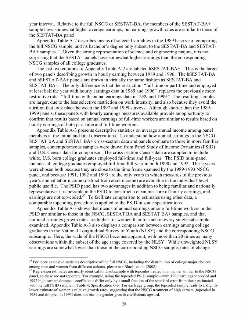
28

year interval. Relative to the full NSCG or SESTAT-BA, the members of the SESTAT-BA+ sample have somewhat higher average earnings, but earnings growth rates are similar to those of the SESTAT-BA panel.

Appendix Table A-2 describes means of selected variables in the 1989 base year, comparing the full NSCG sample, and its bachelor’s degree only subset, to the SESTAT-BA and SESTAT-BA+ samples.36 Given the strong representation of science and engineering majors, it is not surprising that the SESTAT panels have somewhat higher earnings than the corresponding NSCG samples of all college graduates.

The last two columns of Appendix Table A-2 are labeled hSESTAT-BA+ . This is the larger of two panels describing growth in hourly earning between 1989 and 1996. The hSESTAT-BA and hSESTAT-BA+ panels are drawn in virtually the same fashion as SESTAT-BA and SESTAT-BA+. The only difference is that the restriction: “full-time or part-time and employed at least half the year with hourly earnings data in 1989 and 1996” replaces the previously more restrictive rule: “full-time with annual earnings data in 1989 and 1999.” The resulting samples are larger, due to the less selective restriction on work intensity, and also because they avoid the attrition that took place between the 1997 and 1999 surveys. Although shorter than the 1989-1999 panels, these panels with hourly earnings measures available provide an opportunity to confirm that results based on annual earnings of full-time workers are similar to results based on hourly earnings of both part-time and full-time workers.

Appendix Table A-3 presents descriptive statistics on average annual income among panel members at the initial and final observations. To understand how annual earnings in the NSCG, SESTAT BA and SESTAT BA+ cross-section data and panels compare to those in more familiar samples, contemporaneous samples were drawn from Panel Study of Income Dynamics (PSID) and U.S. Census data for comparison. The cross-section Census data are sampled to include white, U.S. born college graduates employed full-time and full-year. The PSID mini-panel includes all college graduates employed full-time full-year in both 1990 and 1992. These years were chosen both because they are close to the time frame spanned by the 1989-1993 NSCG panel, and because 1991, 1992 and 1993 are the only years in which measures of the previous year’s annual labor income (distinct from asset income) are available in the individual-level public use file. The PSID panel has two advantages in addition to being familiar and nationally representative: it is possible in the PSID to construct a clean measure of hourly earnings, and earnings are not top-coded.37 To facilitate comparison to estimates using other data, a comparable topcoding procedure is applied to the PSID in some specifications.

Appendix Table A-3 shows that means of annual earnings among full-time workers in the PSID are similar to those in the NSCG, SESTAT BA and SESTAT BA+ samples, and that nominal earnings growth rates are higher for women than for men in every single subsample examined. Appendix Table A-3 also displays a comparison between earnings among college graduates in the National Longitudinal Survey of Youth (NLSY) and the corresponding NSCG subsample. Here, the scale of the NSCG becomes apparent, with more than 20 times as many observations within the subset of the age range covered by the NLSY. While unweighted NLSY earnings are somewhat lower than those in the corresponding NSCG sample, rates of change

36 For more extensive statistics descriptive of the full NSCG, including the distribution of college major choices among men and women from different cohorts, please see Black, et. al. (2008). 37 Regression estimates are nearly identical for a subsample with topcodes treated in a manner similar to the NSCG panel, so these are not reported. For example, using the topcoded PSID sample—with 1990 earnings topcoded and 1992 high earners dropped--coefficients differ only by a small fraction of the standard error from those estimated with the full PSID sample in Table 4, Specification 6-b. For each age group, the topcoded sample leads to a slightly lower estimate of women’s relative growth rates, suggesting that the NSCG treatment of high earners (topcoded in 1989 and dropped in 1993) does not bias the gender growth coefficients upward.

29

over time are similar: Men’s earnings grow by 29 percent in the NSCG and 30 percent in the NLSY, while women’s earnings grow by 33 percent in the NSCG and 35 percent in the NLSY. This exercise demonstrates that there is nothing unusual about the NSCG earnings measures that might be spuriously driving the results about women’s faster earnings growth.

Appendix Table Table A-1 --Details of selection into the SESTAT-BA and SESTAT-BA+ Panels Selection into

SESTAT-BA Panel Selection into

SESTAT-BA+ Panel Row # men women men women

1

Table 1, Column 2 Sample (White, Age 23-52, U.S. Born, Employed Full-time Full-Year in 1989 with Income at least $2000)

32,132 13,065 32,132 13,065

2

Restricted to bachelor’s degree only (Table 1, Column 5)

20,895 8,850 n/a n/a

3

Restricted to pre-1989 college major in eng, cs, math, sci, soc sci (not 1993 occupation, nor other possibly scientific major)

10,502 2,774 n/a n/a

4

…and surveyed (& responded) after 1993 (conditional)

7,155 1,912 n/a n/a

5

Surveyed (& responded) after 1993 (unconditional)

n/a n/a 13,643 3,770

6 …and no new higher degrees as of 1995

7,057 1,871 13,260 3,646

7 …and responded after 1995

6,614 1,746 12,489 3,447

8 …and no new higher degrees as of 1997

6,528 1,709 12,376 3,393

9 …and responded in 1999

4,928 1,288 9,490 2,615

10 …and no new higher degrees as of 1999

4,876 1,261 9,422 2,582

11 …and working full-time in 1999

4,514 918 8,683 1,907

12 …and 1999 salary data nonmissing

4,486 910 8,628 1,891

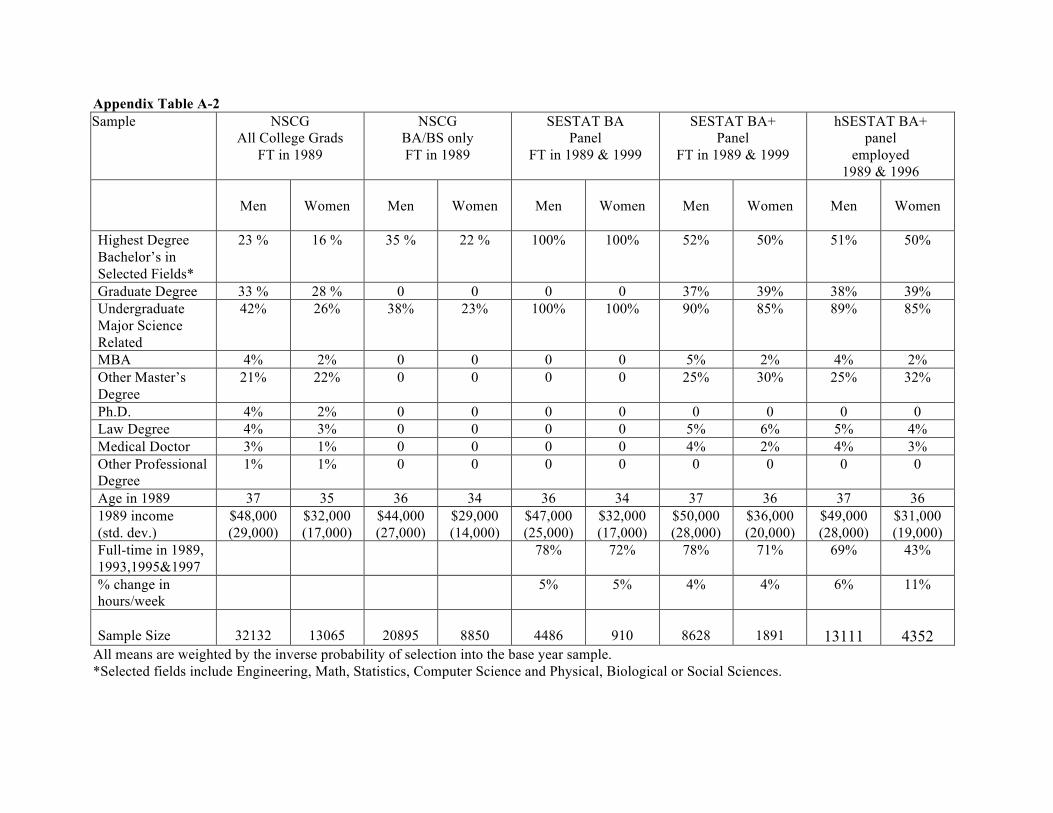
Appendix Table A-2 Sample NSCG

All College Grads FT in 1989

NSCG BA/BS only FT in 1989

SESTAT BA Panel

FT in 1989 & 1999

SESTAT BA+ Panel

FT in 1989 & 1999

hSESTAT BA+ panel

employed 1989 & 1996

Men

Women

Men

Women

Men

Women

Men

Women

Men

Women

Highest Degree Bachelor’s in Selected Fields*

23 % 16 % 35 % 22 % 100% 100% 52% 50% 51% 50%

Graduate Degree 33 % 28 % 0 0 0 0 37% 39% 38% 39% Undergraduate Major Science Related

42% 26% 38% 23% 100% 100% 90% 85% 89% 85%

MBA 4% 2% 0 0 0 0 5% 2% 4% 2% Other Master’s Degree

21% 22% 0 0 0 0 25% 30% 25% 32%

Ph.D. 4% 2% 0 0 0 0 0 0 0 0 Law Degree 4% 3% 0 0 0 0 5% 6% 5% 4% Medical Doctor 3% 1% 0 0 0 0 4% 2% 4% 3% Other Professional Degree

1% 1% 0 0 0 0 0 0 0 0

Age in 1989 37 35 36 34 36 34 37 36 37 36 1989 income (std. dev.)

$48,000 (29,000)

$32,000 (17,000)

$44,000 (27,000)

$29,000 (14,000)

$47,000 (25,000)

$32,000 (17,000)

$50,000 (28,000)

$36,000 (20,000)

$49,000 (28,000)

$31,000 (19,000)

Full-time in 1989, 1993,1995&1997

78% 72% 78% 71% 69% 43%

% change in hours/week

5% 5% 4% 4% 6% 11%

Sample Size

32132

13065

20895

8850

4486

910

8628

1891

13111

4352

All means are weighted by the inverse probability of selection into the base year sample. *Selected fields include Engineering, Math, Statistics, Computer Science and Physical, Biological or Social Sciences.

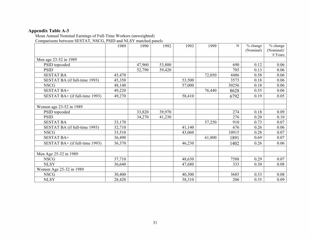
31

Appendix Table A-3 Mean Annual Nominal Earnings of Full-Time Workers (unweighted) Comparisons between SESTAT, NSCG, PSID and NLSY matched panels 1989 1990 1992 1993 1999 N % change

(Nominal) % change

(Nominal)/ # Years

Men age 23-52 in 1989 PSID topcoded 47,960 53,800 690 0.12 0.06 PSID 52,790 59,420 705 0.13 0.06 SESTAT BA 45,470 72,050 4486 0.58 0.06 SESTAT BA (if full-time 1993) 45,350 53,500 3573 0.18 0.06 NSCG 48,140 57,000 30256 0.18 0.06 SESTAT BA+ 49,220 76,440 8628 0.55 0.06 SESTAT BA+ (if full-time 1993) 49,270 58,410 6792 0.19 0.05

Women age 23-52 in 1989 PSID topcoded 33,820 39,970 274 0.18 0.09 PSID 34,270 41,230 276 0.20 0.10 SESTAT BA 33,170 57,250 910 0.73 0.07 SESTAT BA (if full-time 1993) 32,710 41,140 676 0.26 0.06 NSCG 33,510 43,060 10915 0.28 0.07 SESTAT BA+ 36,490 61,800 1891 0.69 0.07 SESTAT BA+ (if full-time 1993) 36,370 46,230 1402 0.26 0.06

Men Age 25-32 in 1989 NSCG 37,710 48,630 7588 0.29 0.07 NLSY 36,640 47,680 333 0.30 0.08

Women Age 25-32 in 1989 NSCG 30,400 40,300 3685 0.33 0.08 NLSY 28,420 38,310 206 0.35 0.09

32

Table 1-- College Graduate Gender Earnings Gaps (1989 Full time, full year workers, college graduates age 23-52). Data from the NSF National Survey of College Graduates, a follow-up survey of college graduates drawn from the 1990 Census

(1) (2) (3) (4) (5) (6) (7)

Year &Sample

1989

Census College

Graduates

1989

NSCG College

Graduates

1989

NSCG College

Graduates

1989

NSCG College

Graduates

1989

NSCG College

Graduates Bachelor’s

degree only

SESTAT-BA

Panel (Also full-

time in 1999) Bachelor’s

degree only

SESTAT-BA+

Panel (Also full-

time in 1999)

Female*(age 23-32) -0.145 -0.135 -0.088 -0.068 -0.077 -0.093 -0.082 (0.005)** (0.009)** (0.009)** (0.009)** (0.010)** (0.027)** (0.022)**

Female*(age 33-42) -0.291 -0.286 -0.224 -0.195 -0.214 -0.208 -0.158 (0.005)** (0.010)** (0.010)** (0.010)** (0.013)** (0.037)** (0.025)**

Female*(age 43-52) -0.459 -0.446 -0.349 -0.309 -0.380 -0.449 -0.331 (0.007)** (0.015)** (0.015)** (0.015)** (0.020)** (0.058)** (0.039)**

Master's Degree 0.082 0.052 0.067 (0.004)** (0.007)** (0.007)**

Ph.D. or Professional 0.245 0.275 0.298 (0.006)** (0.011)** (0.011)**

College Major Controls:

No No Broad college major, level of graduate

degree

Narrow college major,

second majors,

minors, field and level of

graduate degrees

Narrow college major,

second majors, minors

Narrow college major,

second majors, minors

Narrow college major,

second majors,

minors, field and level of

graduate degrees

Observations 118123 45197 45197 45197 29745 5396 10519 R-squared 0.25 0.26 0.31 0.35 0.32 0.32 0.33

(notes on next page) * significant at 5%; ** significant at 1%

33

Table 1 notes: Sample, Columns 1-4: White college graduates age 23-52, born in the U.S., employed full time, full year (at least 50 weeks, usual hours/week at least 35), annual income at least $2000 from Census (Column 1) or NSCG (Columns 2-4). Column 5 further restrict the NSCG sample to bachelor’s level graduates only, and column 6 to bachelor’s level graduates with selected college majors who were resurveyed, working full-time, and had no graduate degrees in 1999 (SESTAT-BA Panel), Column 7 SESTAT-BA+ Panel. See Data Appendix for complete description of panel samples.

. Dependent Variable: Log of annual wage and salary income as reported in 1990 Census; College major controls: Column 3: 9 broad categories, Column 4: Detailed college majors (156 categories), 8 categories of college minor or second major, 9 categories of master’s degree, 5 categories of Ph.D., and 4 categories of professional license, Column 5: Detailed college majors (146 categories), 8 categories of college minor or second major, Column 6: Detailed college majors (71 categories), 8 categories of college minor or second major. Column 7: Detailed college majors (145 categories), 8 categories of college minor or second major, 9 categories of master’s degree, and 2 categories of professional license. Additional controls included in all regressions: 35-39, 41-48, and 49+ hours/week, geographic controls for 9 census divisions, age controls for 30 possible ages.

34

Table 2-- College Graduate Gender Earnings Gaps by Field of College Major (1989 Full time, full year workers, bachelor’s level college graduates age 23-52) . Data from the National Survey of College Graduates.

(1) (2) (3) (4) (5) (6) (7) (8)

Compsci Engin Math/Sci SocSci Bus Hum Educ Health

Female*(age 23-32) 0.017 -0.052 -0.060 -0.114 -0.103 -0.118 -0.092 -0.098 (0.027) (0.024)* (0.035) (0.034)** (0.017)** (0.049)* (0.039)* (0.051)

Female*(age 33-42) -0.090 -0.058 -0.158 -0.219 -0.231 -0.195 -0.276 -0.231 (0.067) (0.054) (0.040)** (0.038)** (0.036)** (0.044)** (0.034)** (0.045)**

Female*(age 43-52) suppressed -0.443 -0.401 -0.387 -0.404 -0.336 -0.386 -0.136 (0.284) (0.171)** (0.067)** (0.060)** (0.068)** (0.059)** (0.055)** (0.084)

Number of College Majors

7 22 26 16 9 7 13 11

Observations 1408 5917 3254 2666 6287 1913 2029 1133 R-squared 0.28 0.27 0.31 0.28 0.27 0.26 0.25 0.25

Detailed # Observations:

Men, age 23-32 773 2561 717 464 1820 266 162 80 Men, age 33-42 209 1828 1053 831 1863 563 461 144 Men, age 43-52 36 1090 555 361 1060 291 226 55

Women, age 23-32 325 375 436 491 1166 271 317 398 Women, age 33-42 63 57 357 381 303 320 527 332 Women, age 43-52 suppressed 6 136 138 75 202 336 124

* significant at 5%; ** significant at 1% Sample: White bachelor’s level college graduates age 23-52, born in the U.S., employed full time, full year (at least 50 weeks, usual hours/week at least 35), annual income at least $2000. Dependent Variable: Log of annual wage and salary income as reported in 1990 Census. Additional controls included in all regressions: detailed college major fixed effects, 8 categories of college minor or second major, controls for 35-39, 41-48, and 49+ hours/week, geographic controls for 9 census divisions, age controls for 30 possible ages. Information based on cell size less than 5 has been suppressed at the request of the National Science Foundation Division of Science Resource Statistics. The coefficient estimate in the “suppressed” cell has magnitude less than 1/3 of the standard error.

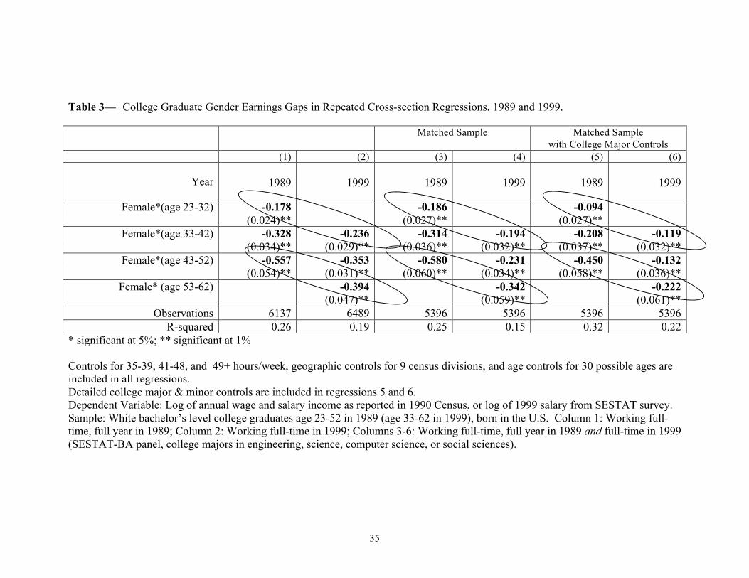
35

Table 3— College Graduate Gender Earnings Gaps in Repeated Cross-section Regressions, 1989 and 1999.

Matched Sample Matched Sample with College Major Controls

(1) (2) (3) (4) (5) (6)

Year

1989

1999

1989

1999

1989

1999

Female*(age 23-32) -0.178 -0.186 -0.094 (0.024)** (0.027)** (0.027)**

Female*(age 33-42) -0.328 -0.236 -0.314 -0.194 -0.208 -0.119 (0.034)** (0.029)** (0.036)** (0.032)** (0.037)** (0.032)**

Female*(age 43-52) -0.557 -0.353 -0.580 -0.231 -0.450 -0.132 (0.054)** (0.031)** (0.060)** (0.034)** (0.058)** (0.036)**

Female* (age 53-62) -0.394 -0.342 -0.222 (0.047)** (0.059)** (0.061)**

Observations 6137 6489 5396 5396 5396 5396 R-squared 0.26 0.19 0.25 0.15 0.32 0.22

* significant at 5%; ** significant at 1% Controls for 35-39, 41-48, and 49+ hours/week, geographic controls for 9 census divisions, and age controls for 30 possible ages are included in all regressions. Detailed college major & minor controls are included in regressions 5 and 6. Dependent Variable: Log of annual wage and salary income as reported in 1990 Census, or log of 1999 salary from SESTAT survey. Sample: White bachelor’s level college graduates age 23-52 in 1989 (age 33-62 in 1999), born in the U.S. Column 1: Working full-time, full year in 1989; Column 2: Working full-time in 1999; Columns 3-6: Working full-time, full year in 1989 and full-time in 1999 (SESTAT-BA panel, college majors in engineering, science, computer science, or social sciences).

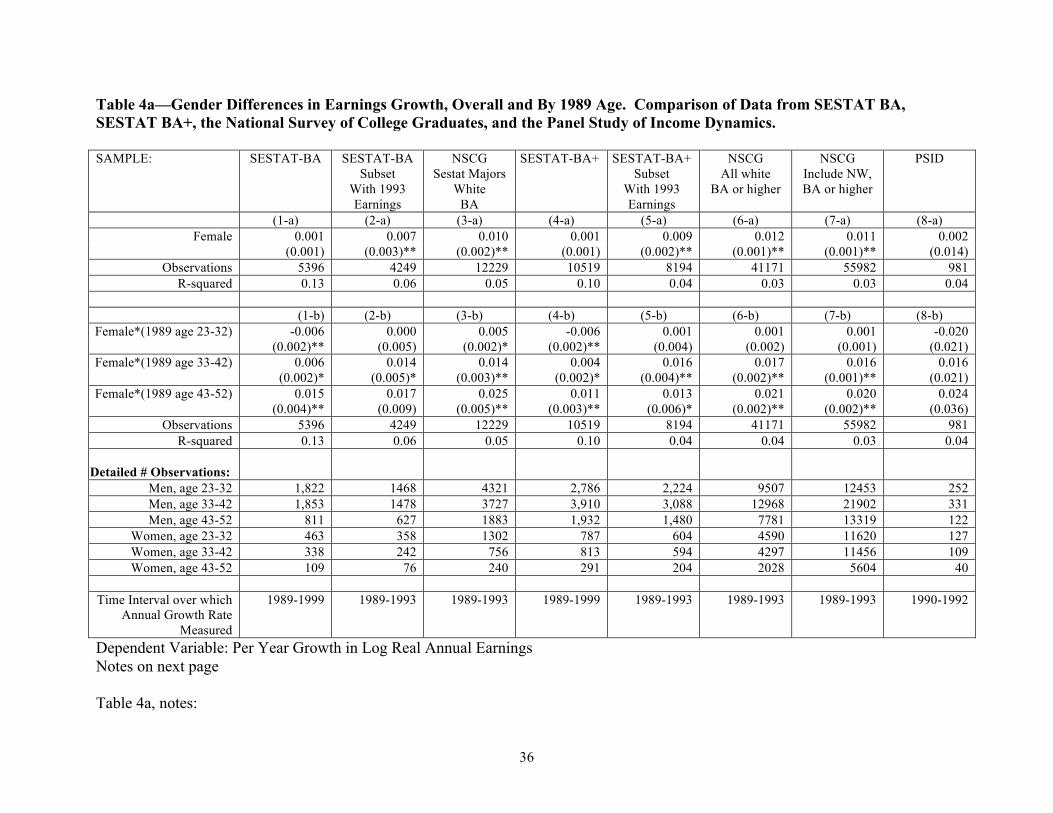
36

Table 4a—Gender Differences in Earnings Growth, Overall and By 1989 Age. Comparison of Data from SESTAT BA, SESTAT BA+, the National Survey of College Graduates, and the Panel Study of Income Dynamics. SAMPLE: SESTAT-BA SESTAT-BA

Subset With 1993 Earnings

NSCG Sestat Majors

White BA

SESTAT-BA+ SESTAT-BA+ Subset

With 1993 Earnings

NSCG All white

BA or higher

NSCG Include NW, BA or higher

PSID

(1-a) (2-a) (3-a) (4-a) (5-a) (6-a) (7-a) (8-a) Female 0.001 0.007 0.010 0.001 0.009 0.012 0.011 0.002

(0.001) (0.003)** (0.002)** (0.001) (0.002)** (0.001)** (0.001)** (0.014) Observations 5396 4249 12229 10519 8194 41171 55982 981

R-squared 0.13 0.06 0.05 0.10 0.04 0.03 0.03 0.04 (1-b) (2-b) (3-b) (4-b) (5-b) (6-b) (7-b) (8-b) Female*(1989 age 23-32) -0.006 0.000 0.005 -0.006 0.001 0.001 0.001 -0.020

(0.002)** (0.005) (0.002)* (0.002)** (0.004) (0.002) (0.001) (0.021) Female*(1989 age 33-42) 0.006 0.014 0.014 0.004 0.016 0.017 0.016 0.016

(0.002)* (0.005)* (0.003)** (0.002)* (0.004)** (0.002)** (0.001)** (0.021) Female*(1989 age 43-52) 0.015 0.017 0.025 0.011 0.013 0.021 0.020 0.024 (0.004)** (0.009) (0.005)** (0.003)** (0.006)* (0.002)** (0.002)** (0.036)

Observations 5396 4249 12229 10519 8194 41171 55982 981 R-squared 0.13 0.06 0.05 0.10 0.04 0.04 0.03 0.04

Detailed # Observations:

Men, age 23-32 1,822 1468 4321 2,786 2,224 9507 12453 252 Men, age 33-42 1,853 1478 3727 3,910 3,088 12968 21902 331 Men, age 43-52 811 627 1883 1,932 1,480 7781 13319 122

Women, age 23-32 463 358 1302 787 604 4590 11620 127 Women, age 33-42 338 242 756 813 594 4297 11456 109 Women, age 43-52 109 76 240 291 204 2028 5604 40

Time Interval over which

Annual Growth Rate Measured

1989-1999 1989-1993 1989-1993 1989-1999 1989-1993 1989-1993 1989-1993 1990-1992

Dependent Variable: Per Year Growth in Log Real Annual Earnings Notes on next page Table 4a, notes:

37

Controls: complete set of controls for exact year of age Sample: College graduates age 23-52 employed full-time at beginning and end of interval. Additional sample restrictions are indicated for each column. Column 1 is the SESTAT-BA sample, with earnings growth measured 1989-1999. Columns 2-3 measure earnings growth over the shorter 1989-1993 window. Column 2 is the subset of SESTAT-BA for which a 1989-1993 earnings growth measure is available. Column 3 is a subset of the NSCG with SESTAT-like sample restrictions imposed (e.g. white, U.S. born, bachelor’s degree only majors in engineering, science or social sciences). Columns 4 and 5 are similar to columns 1 and 2, but using the larger SESTAT-BA+ sample including graduates with higher degrees. Column 6 is similar to column 3, but covers all white college graduates with no college major restrictions, and including graduates with higher degrees. Column 7 includes all NSCG observations on college graduates (not restricted to white graduates). Column 8 includes all PSID college graduates, with earnings growth measured 1990-1992. Table 4b notes: Controls: complete set of controls for exact year of age Sample: College graduates age 23-52 employed in 1989 and 1996. Additional sample restrictions are indicated for each column. Column 9 is the hSESTAT-BA sample, including both part-time and full-time workers. Columns 10 and 11 restrict the hSESTAT-BA to workers employed full-time, full-year in both 1989 and 1996 (slight difference in sample is because workers with hourly earnings below $1 or annual earnings below $2000 were dropped). Columns 12 is the hSESTAT-BA+ sample, and columns 13-14 restrict the hSESTAT-BA+ sample to workers employed full-time, full-year in both 1989 and 1996. note: Consistently Part-Time Worker is defined as working less than 35 hours per week in 1986, 1996 and at least one observation in between.

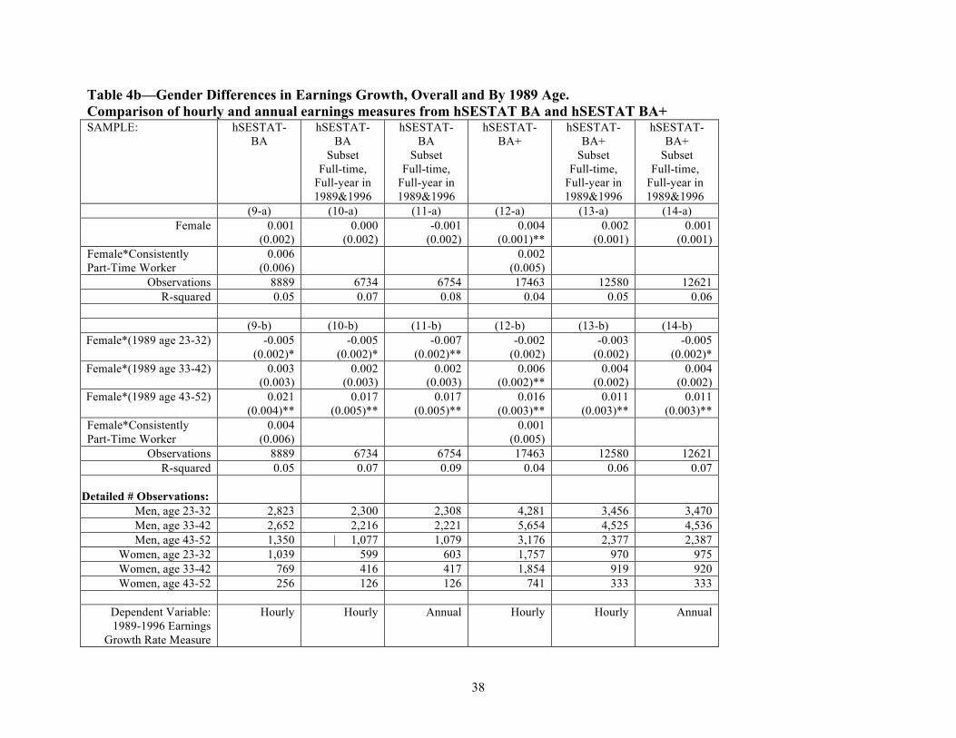
38

Table 4b—Gender Differences in Earnings Growth, Overall and By 1989 Age. Comparison of hourly and annual earnings measures from hSESTAT BA and hSESTAT BA+ SAMPLE: hSESTAT-

BA hSESTAT-

BA Subset

Full-time, Full-year in 1989&1996

hSESTAT-BA

Subset Full-time,

Full-year in 1989&1996

hSESTAT-BA+

hSESTAT-BA+

Subset Full-time,

Full-year in 1989&1996

hSESTAT-BA+

Subset Full-time,

Full-year in 1989&1996

(9-a) (10-a) (11-a) (12-a) (13-a) (14-a) Female 0.001 0.000 -0.001 0.004 0.002 0.001

(0.002) (0.002) (0.002) (0.001)** (0.001) (0.001) Female*Consistently 0.006 0.002 Part-Time Worker (0.006) (0.005)

Observations 8889 6734 6754 17463 12580 12621 R-squared 0.05 0.07 0.08 0.04 0.05 0.06

(9-b) (10-b) (11-b) (12-b) (13-b) (14-b) Female*(1989 age 23-32) -0.005 -0.005 -0.007 -0.002 -0.003 -0.005

(0.002)* (0.002)* (0.002)** (0.002) (0.002) (0.002)* Female*(1989 age 33-42) 0.003 0.002 0.002 0.006 0.004 0.004

(0.003) (0.003) (0.003) (0.002)** (0.002) (0.002) Female*(1989 age 43-52) 0.021 0.017 0.017 0.016 0.011 0.011 (0.004)** (0.005)** (0.005)** (0.003)** (0.003)** (0.003)** Female*Consistently 0.004 0.001 Part-Time Worker (0.006) (0.005)

Observations 8889 6734 6754 17463 12580 12621 R-squared 0.05 0.07 0.09 0.04 0.06 0.07

Detailed # Observations:

Men, age 23-32 2,823 2,300 2,308 4,281 3,456 3,470 Men, age 33-42 2,652 2,216 2,221 5,654 4,525 4,536 Men, age 43-52 1,350 | 1,077 1,079 3,176 2,377 2,387

Women, age 23-32 1,039 599 603 1,757 970 975 Women, age 33-42 769 416 417 1,854 919 920 Women, age 43-52 256 126 126 741 333 333

Dependent Variable: 1989-1996 Earnings

Growth Rate Measure

Hourly Hourly Annual Hourly Hourly Annual

39

Table 5—Gender Differences in Earnings Growth, by Highest College Degree and Age in 1989. Data from the National Survey of College Graduates.

Bachelor’s Degree

Master’s Degree

Ph.D.

(1) (2) (3) (4) (5) (6) Female*(age 23-32) 0.007 0.003 0.006 -0.002 0.025 0.017

(0.002)** (0.002) (0.004) (0.004) (0.014) (0.016) Female*(age 33-42) 0.012 0.017 0.014 0.016 -0.004 -0.003

(0.002)** (0.002)** (0.002)** (0.003)** (0.007) (0.007) Female*(age 43-52) 0.027 0.022 0.024 0.020 0.018 0.019

(0.003)** (0.003)** (0.003)** (0.003)** (0.008)* (0.008)* Age (in decades) -0.023 -0.020 -0.029

(0.001)** (0.001)** (0.004)** Constant 0.013 0.020 0.041

(0.001)** (0.001)** (0.004)** Additional Controls No Yes No Yes No Yes

Observations 26900 26900 9677 9677 1931 1931

R-squared 0.04 0.04 0.03 0.04 0.04 0.07 * significant at 5%; ** significant at 1% Dependent Variable: Growth per year in log real annual earnings 1989 to 1993. Additional controls: Detailed field of degree and exact age fixed effects included in even columns. Constant evaluated at age 32 in odd-numbered columns. Sample: White college graduates age 23-52, born in the U.S., employed full time, full year in 1989 and full-time in 1993.

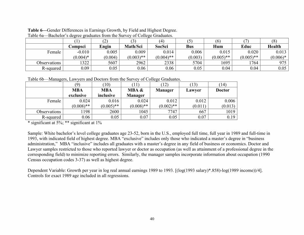
40

Table 6—Gender Differences in Earnings Growth, by Field and Highest Degree. Table 6a—Bachelor’s degree graduates from the Survey of College Graduates. (1) (2) (3) (4) (5) (6) (7) (8) Compsci Engin Math/Sci SocSci Bus Hum Educ Health

Female -0.010 0.005 0.009 0.014 0.006 0.015 0.020 0.013 (0.004)* (0.004) (0.003)** (0.004)** (0.003) (0.005)** (0.005)** (0.006)*

Observations 1322 5607 2962 2338 5704 1695 1764 975 R-squared 0.09 0.05 0.06 0.06 0.05 0.04 0.04 0.05

Table 6b—Managers, Lawyers and Doctors from the Survey of College Graduates. (9) (10) (11) (12) (13) (14) MBA

exclusive MBA

inclusive MBA & Manager

Manager Lawyer Doctor

Female 0.024 0.016 0.024 0.012 0.012 0.006 (0.008)** (0.005)** (0.008)** (0.002)** (0.011) (0.013)

Observations 1198 2600 1045 7747 667 1019 R-squared 0.06 0.05 0.07 0.05 0.07 0.19

* significant at 5%; ** significant at 1% Sample: White bachelor’s level college graduates age 23-52, born in the U.S., employed full time, full year in 1989 and full-time in 1993, with indicated field of highest degree. MBA “exclusive” includes only those who indicated a master’s degree in “business administration,” MBA “inclusive” includes all graduates with a master’s degree in any field of business or economics. Doctor and Lawyer samples restricted to those who reported lawyer or doctor as occupation (as well as attainment of a professional degree in the corresponding field) to minimize reporting errors. Similarly, the manager samples incorporate information about occupation (1990 Census occupation codes 3-37) as well as highest degree. Dependent Variable: Growth per year in log real annual earnings 1989 to 1993. [(log(1993 salary)*.858)-log(1989 income))/4]. Controls for exact 1989 age included in all regressions.

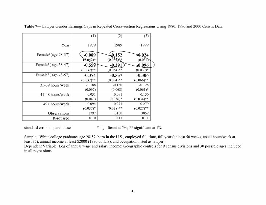
41

Table 7— Lawyer Gender Earnings Gaps in Repeated Cross-section Regressions Using 1980, 1990 and 2000 Census Data.

(1) (2) (3)

Year

1979

1989

1999

Female*(age 28-37) -0.089 -0.152 -0.024 (0.042)* (0.031)** (0.034)

Female*( age 38-47) -0.559 -0.291 -0.096 (0.132)** (0.054)** (0.039)*

Female*( age 48-57) -0.374 -0.557 -0.306 (0.132)** (0.094)** (0.066)**

35-39 hours/week -0.188 -0.130 -0.128 (0.097) (0.068) (0.061)*

41-48 hours/week 0.031 0.091 0.150 (0.043) (0.036)* (0.034)**

49+ hours/week 0.094 0.273 0.279 (0.037)* (0.028)** (0.027)**

Observations 1797 3160 3859

R-squared 0.10 0.13 0.11

standard errors in parentheses * significant at 5%; ** significant at 1% Sample: White college graduates age 28-57, born in the U.S., employed full time, full year (at least 50 weeks, usual hours/week at least 35), annual income at least $2000 (1990 dollars), and occupation listed as lawyer. Dependent Variable: Log of annual wage and salary income; Geographic controls for 9 census divisions and 30 possible ages included in all regressions.

42

Table 8—Further Analysis of Gender Differences in Earnings Growth, Using Contemporaneous Measures of Observable Characteristics in SESTAT-BA Panel Data

(1) (2) (3) (4) (5) (6) Female*(1989 age 23-32) -0.006 -0.006 -0.006 -0.006 -0.007 -0.005

(0.002)** (0.002)** (0.002)** (0.002)** (0.003)* (0.003) Female*(1989 age 33-42) 0.006 0.006 0.007 0.006 0.003 0.001

(0.002)* (0.002)* (0.002)** (0.002)** (0.003) (0.003) Female*(1989 age 43-52) 0.015 0.015 0.015 0.015 0.006 0.002

(0.004)** (0.004)** (0.004)** (0.004)** (0.005) (0.005) % change in hours per 0.016

week if increase (0.004)** % change in hours per 0.058

week if decrease (0.007)** Not full-time -0.006

all years (0.001)** Not full-time all years -0.007

*(1989 age 23-32) (0.002)** Not full-time all years -0.004

*(1989 age 33-42) (0.002)* Not full-time all years -0.007

*(1989 age 43-52) (0.003)* Mother in 89, 0.017 0.020

Empty nest in 99 (0.005)* (0.005)** Mother in 89, 0.003

Still kids at home 99 (0.003) New Mother in 99, -0.002 -0.001

No kids in 89 (0.004) (0.004) Mother in 89, 0.005

Young kids home 99 (0.005) Mother in 89, only 0.007

Teens 12+ home 99 (0.005) Mother in 89, only 0.011 Older teens 18+ 99 (0.007) Observed as Young -0.008

Mother (0.005) Observations 5396 5396 5396 5396 5396 5396

R-squared 0.13 0.15 0.13 0.13 0.13 0.13 * significant at 5%; ** significant at 1% Dependent Variable: Growth per year in log real annual earnings 1989 to 1999 ((ln(1999 real earnings)-ln(1989 real earnings))/10 . Sample: SESTAT-BA (see data appendix for detailed description) Those who worked “full-time all years” also worked full-time in 1993, 1995 and 1997. Age dummies spanning 30 possible ages included in all regressions Omitted parenting category: Women (the same age) with no births as of 1990, no older children in 1993, and no kids reported living at home in 1999. Column 6 categories of parenting in both 1989 and 1999 are mutually exclusive (all children are younger than 12 in 1999, all children are at least 18 in 1999, or all children are at least 12, but at least one child is less than 18 in 1999). Young mother flags women in the 23-32 age group with children in 1989, plus those with new children observed in 1993, 1995 or 1997 who are 32 or younger at the time of observation.

43

Table 9—Earnings Growth of Mothers and Non-mothers, Relative to Men the Same Age, by Age Group (Change in Log Annual Full-Time Earnings 1989-1999 SESTAT-BA, and Change in Log Hourly Earnings Full-Time or Part-Time 1989-1996 hSESTAT-BA+) (1) (2) (3) (4) (5)

1989 Age 23-32 33-42 43-52 23-52 23-42 1999 Age 33-42 43-52 53-62 33-62 33-52

SESTAT-BA Sample

Mother -0.009 0.011 0.021 0.003 -0.000 (0.003)** (0.003)** (0.005)** (0.002) (0.002) Non-Mother -0.003 -0.001 -0.005 -0.002 -0.002 (0.003) (0.004) (0.009) (0.002) (0.002) Observations 2285 2191 920 5396 4476 R-squared 0.07 0.02 0.03 0.13 0.12 # Mothers 258 199 84 541 457 # Non-Mothers 205 139 25 369 344 Proportion of mothers not full-time all years

0.25

0.33

0.36

Proportion of non-mothers not full-time all years

0.28

0.27

0.28

hSESTAT-BA+

Mother -0.003 0.007 0.020 0.006 0.003 (0.002) (0.002)** (0.003)** (0.001)** (0.002) Non-Mother -0.002 0.005 0.001 0.002 0.003 (0.003) (0.003) (0.006) (0.002) (0.002) Observations 6038 7508 3917 17463 13546 R-squared 0.01 0.01 0.01 0.04 0.03 # Mothers 1169 1230 575 2974 2399 # Non-Mothers 588 624 166 1378 1212

Dependent Variable: SESTAT-BA: Growth per year in log annual earnings 1989 to 1999 ((ln(1999 real earnings)-ln(1989 real earnings))/10 hSESTAT-BA+: Growth per year in log hourly earnings 1989 to 1996 ((ln(1996 real hourly earnings)-ln(1989 real hourly earnings))/7 Those who worked “full-time all years” were also observed working full-time in 1993, 1995 and 1997. Age dummies spanning all possible ages included in each regression. Mother is defined as a woman with positive fertility as of the 1990 Census, or children in any observation through 1999. Non-mothers are all remaining women.

44

Table 10— Quantile Regresssion By Age Cohort, Gender and 1995 Salary Quintile Quantile: .5 .75 .85 .95 SESTAT BA+ 1989-1999

(1-a) (2-a) (3-a) (4-a) Female*(Salary95>80k) 0.010 0.003 -0.006 -0.032

(0.003)** (0.004) (0.004) (0.011)** Female*(Salary95<80k) 0.005 0.007 0.011 0.013

(0.001)** (0.001)** (0.001)** (0.005)** (Salary95>80k) 0.004 0.011 0.018 0.038

(0.001)** (0.001)** (0.001)** (0.005)** Observations 10085 10085 10085 10085

SESTAT BA+ 1989-1999

(1-b) (2-b) (3-b) (4-b) Female*(Salary95>80k) 0.005 0.002 -0.004 -0.020

(0.002)* (0.003) (0.003) (0.009)* Female*(Salary95<80k) 0.005 0.007 0.011 0.014

(0.001)** (0.001)** (0.001)** (0.004)** Observations 10085 10085 10085 10085

Age 23-32

(1-c) (2-c) (3-c) (4-c) Female*(Salary95>70k) -0.011 -0.017 -0.026 -0.049

(0.006) (0.006)** (0.008)** (0.016)** Female*(Salary95<70k) -0.000 0.002 0.004 0.008

(0.002) (0.003) (0.004) (0.010) (Salary95>70k) 0.017 0.027 0.032 0.051

(0.003)** (0.003)** (0.004)** (0.011)** Observations 3424 3424 3424 3424

Age 33-52

(1-d) (2-d) (3-d) (4-d) Female*(Salary95>85k) 0.014 0.010 0.006 -0.023

(0.004)** (0.005)* (0.005) (0.017) Female*(Salary95<85k) 0.008 0.009 0.013 0.015

(0.001)** (0.002)** (0.002)** (0.007)* (Salary95>85k) 0.001 0.006 0.013 0.028

(0.001) (0.002)** (0.002)** (0.006)** Observations 6661 6661 6661 6661

Dependent Variable: Per Year Growth in Log Real Annual Earnings, 1989-1999. Sample: SESTAT BA+ restricted to those employed full-time in 1995, with 1995 salary data available. Detailed number of observations (all ages, 23-32, 33-52): Female and high salary: n=151, 85, 91; Male and and high salary: n=1528, 634, 934; Female lower salary: n=1593, 441, 1082; Male lower salary: n=6813, 2264, 4554. Age dummies spanning 30 possible ages included in all regressions; specifications 1-b through 4-b include dummies spanning 60 categories of age*(Salary95>80k). Note: In the 33-52 age group, 38 percent of men and 43 percent of women earning more than $85,000 per year in 1995 had topcoded 1999 earnings. Therefore, the growth estimates for this group are only suggestive. Among those with lower 1995 earnings, topcodes affected fewer than 2 percent of men and less than a half-percent of women. (Among the 653 workers with topcoded 1999 earnings, 60 percent were men age 33-52 with high 1995 earnings).

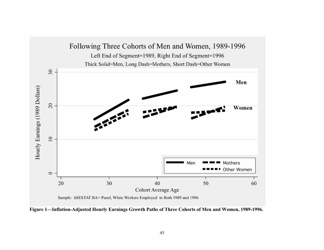
45

Figure 1—Inflation-Adjusted Hourly Earnings Growth Paths of Three Cohorts of Men and Women, 1989-1996.

Women

Men

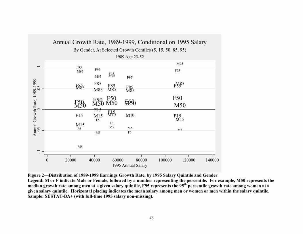
46

Figure 2—Distribution of 1989-1999 Earnings Growth Rate, by 1995 Salary Quintile and Gender Legend: M or F indicate Male or Female, followed by a number representing the percentile. For example, M50 represents the median growth rate among men at a given salary quintile, F95 represents the 95th percentile growth rate among women at a given salary quintile. Horizontal placing indicates the mean salary among men or women or men within the salary quintile. Sample: SESTAT-BA+ (with full-time 1995 salary non-missing).

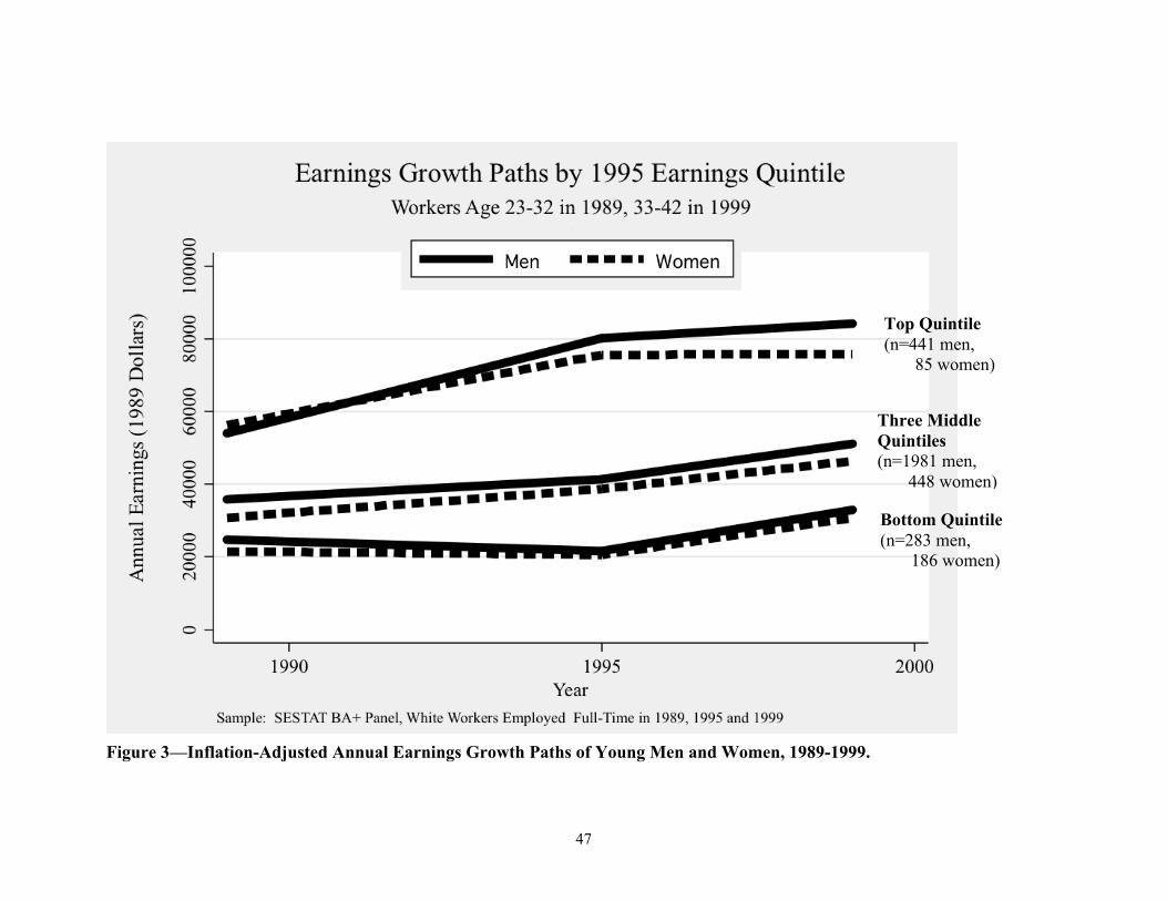
47

Figure 3—Inflation-Adjusted Annual Earnings Growth Paths of Young Men and Women, 1989-1999.

Top Quintile (n=441 men, 85 women)

Bottom Quintile (n=283 men, 186 women)

Three Middle Quintiles (n=1981 men, 448 women)