IN PURSUIT OF BALANCE: RANDOMIZATION IN PRACTICE IN DEVELOPMENT FIELD EXPERIMENTS#

Miriam Bruhn, World Bank

Email: mbruhn@worldbank.org

David McKenzie, World Bank, BREAD, CReAM and IZA Email: dmckenzie@worldbank.org

Abstract We present new evidence on the randomization methods used in existing experiments, and new simulations comparing these methods. We find that many papers do not describe the randomization in detail, implying that better reporting is needed. Our simulations suggest that in samples of 300 plus, the different methods perform similarly. However, for very persistent outcome variables and in smaller samples pair-wise matching and stratification perform best and appear to dominate the re-randomization methods commonly used in practice. The simulations also point to specific recommendations for which variables to balance on and for which controls to include in the ex-post analysis. Keywords: Randomized experiment; Program evaluation; Development. JEL codes: C93, O12.

# We thank the leading researchers in development field experiments who participated in our short survey, as well as colleagues who have shared their experiences with implementing randomization. We thank Angus Deaton, Esther Duflo, David Evans, Xavier Gine, Guido Imbens, Ben Olken and seminar participants at the World Bank for helpful comments, We are also grateful to Radu Ban for sharing his pair-wise matching Stata code, Jishnu Das for the LEAPS data, and to Kathleen Beegle and Kristen Himelein for providing us with their constructed IFLS data.. All views are of course our own.

- 1 -

1. Introduction Randomized experiments are increasingly used in development economics. Historically,

many randomized experiments were large-scale government-implemented social experiments,

such as Moving To Opportunity in the U.S. or Progresa/Oportunidades in Mexico. These

experiments allowed for little involvement of researchers in the actual randomization. In

contrast, in recent years many experiments have been directly implemented by researchers

themselves, or in partnership with NGOs and the private sector. These small-scale experiments,

with sample sizes often comprising 100 to 500 individuals, or 20 to 100 schools or health clinics,

have greatly expanded the range of research questions that can be studied using experiments, and

have provided important and credible evidence on a range of economic and policy issues.

Nevertheless, this move towards smaller sample sizes means researchers increasingly face the

question of not just whether to randomize, but how to do so. This paper provides the first

comprehensive look at how researchers are actually carrying out randomizations in development

field experiments, and then analyzes some of the consequences of these choices.

Simple randomization ensures the allocation of treatment to individuals or institutions is

left purely to chance, and is thus not systematically biased by deliberate selection of individuals

or institutions into the treatment. Randomization thus ensures that the treatment and control

samples are, in expectation, similar in average, both in terms of observed and unobserved

characteristics. Furthermore, it is often argued that the simplicity of experiments offers

considerable advantage in making the results convincing to other social scientists and

policymakers and that, in some instances, random assignment is the fairest and most transparent

way of choosing the recipients of a new pilot program (Burtless, 1995).

However, it has long been recognized that while pure random assignment guarantees that

the treatment and control groups will have identical characteristics on average, in any particular

random allocation, the two groups will differ along some dimensions, with the probability that

such differences are large falling with sample size.1 Although ex-post adjustment can be made

for such chance imbalances, this is less efficient than achieving ex-ante balance, and can not be

used in cases where all individuals with a given characteristic are allocated to just the treatment

group. 1 For example, Kernan et al. (1999) consider a binary variable that is present in 30 percent of the sample. They show that the chance that the two treatment group proportions will differ by more than 10 percent is 38% in an experiment with 50 individuals, 27% in an experiment with 100 individuals, 9% for an experiment with 200 individuals, and 2% for an experiment with 400 individuals.

- 2 -

The standard approach to avoiding imbalance on a few key variables is stratification (or

blocking), originally proposed by R.A. Fisher. Under this approach, units are randomly assigned

to treatment and control within strata defined by usually one or two observed baseline

characteristics. However, in practice it is unlikely that one or two variables will explain a large

share of the variation in the outcome of interest, leading to attempts to balance on multiple

variables. One such method when baseline data are available is pair-wise matching (Greevy et al,

2004, Imai et al. 2007).

The methods of implementing randomization have historically been poorly reported in

medical journals, leading to the formulation of the CONSORT guidelines which set out standards

for the reporting of clinical trials (Schulz, 1996). The recent explosion of field experiments in

development economics has not yet met these same standards, with many papers omitting key

details of the method in which randomization is implemented. For this reason, we conducted a

survey of leading researchers carrying out randomized experiments in developing countries. This

reveals common use of methods to improve baseline balance, including several re-randomization

methods not discussed in print. These are (i) carrying out an allocation to treatment and control,

and then using a statistical threshold or ad hoc procedure to decide whether or not to redraw the

allocation; and (ii) drawing 100 or 1000 allocations to treatment and control, and choosing the

one amongst them which shows best balance on a set of observable variables.

This paper discusses the pros and cons of these different methods for striving towards

balance on observables. Proponents of methods such as stratification, matching, and

minimization claim that such methods can improve efficiency, increase power, and protect

against type I errors (Kernan et al., 1999) and do not seem to have significant disadvantages,

except in small samples (Imai et al. 2008, Greevy et al. 2004, Aickin, 2001)2. However, it is

precisely in small samples that the choice of randomization method becomes important, since in

large samples all methods will achieve balance. We simulate different randomization methods in

four panel data sets. We then compare balance in outcome variables at baseline and at follow-up.

The simulations show that when methods other than pure randomization are used, the degree of

balance achieved on baseline variables is much greater than that achieved on the outcome

variable (in the absence of treatment) in the follow-up period. The simulations show further that

2 One other argument in favor of ex-ante balancing is that, if the treatment effect is heterogeneous and varies with observed covariates, ex-ante balancing increases the precision of subgroup analysis.

- 3 -

in samples of 300 observations or more, the choice of method is not very important for the

degree of balance in many outcomes at follow-up. In small samples, and with very persistent

outcomes, however, matching or stratification on relevant baseline variables achieves more

balance in follow-up outcomes than does pure randomization.

We use our simulation results and theory to help answer many of the important practical

questions facing researchers engaged in randomized experiments. The results allow us to provide

guidance on how to conduct inference after stratification, matching or re-randomization. In

practice it appears that many researchers ignore the method of randomization in inference. We

show that this leads to hypothesis tests with incorrect size. On average, the standard errors are

overly conservative when the method of randomization is not controlled for in the analysis,

implying that researchers may not detect treatment effects that they would detect if the inference

did take into account the randomization method. However, although this is the case on average,

in a non-trivial proportion of draws, it will be the case that not controlling for the randomization

method will result in larger standard errors than if the randomization method is controlled for.

Thus it is possible that not controlling for the randomization method could lead the researcher to

find a significant effect that is no longer significant when stratum or pair dummies are included.

Moreover, we show further that stratifying, matching, or re-randomizing and then analyzing the

data without controlling for the method of randomization results in lower power than if a pure

random draw was used to allocate treatments, except in cases where the variables that balance is

sought for have no predictive power for the future outcome of interest (in which case there is no

need to seek balance on them anyway).

The paper also discusses the use and abuse of tests for baseline differences in means, the

impact of balancing observables on achieving balance on unobservables, and the issue of how

many (and which) variables to use for stratifying or matching. Finally, based on our simulation

results and the previous econometric literature, this paper provides a list of actionable

recommendations for researchers performing and reporting on randomized experiments.

This paper draws upon a large clinical trials literature, where many related issues have

been under discussion for several decades, drawing out the lessons for development field

experiments. It complements several recent papers in development on randomized experiments.3

3 Summaries of recent experiments and advocacy of the policy case are found in Kremer (2003), Duflo and Kremer (2004), Duflo (2005) and Banerjee (2007).

- 4 -

The paper builds on the recent handbook chapter by Duflo, Glennerster and Kremer (2006),

which aims to provide a “how to” of implementing experiments. Our focus differs, considering

how the actual randomization is implemented in practice, and considering matching and re-

randomization approaches. Finally, we contribute to the existing literature through new

simulations which illustrate the performance of the different methods in a variety of situations

experienced in practice.

Whilst our focus is on field experiments in development economics, to date the field with

most active involvement of researchers in randomization, randomized experiments are also

increasingly being used to investigate important policy questions in other fields (Levitt and List,

2008). In common with the development literature, the extant literature in these other fields has

often not explained the precise mechanism used for randomizing. However, it does appear that

re-randomization methods are also being employed in some of these studies. The ongoing New

York public schools project being undertaken by the American Inequality Lab is one such high-

profile example. The lessons of this paper will also be important in designing upcoming

experiments in other fields of economics.

The remainder of the paper is set out as follows. Section 2 provides a stocktaking of how

randomization is currently being implemented, drawing on a summary of papers and a survey of

leading experts in development field experiments. Section 3 describes the data sets used in our

simulations, and outlines in more detail the different methods of randomization. Section 4 then

provides simulation evidence on the relative performance of the different methods, and on

answers to key questions faced in practice. Section 5 concludes with our recommendations.

2. How is randomization being implemented?

2.1. Randomization as described in papers

We begin by reviewing a selection of research papers containing randomized experiments in

development economics. Table 1 summarizes a selection of relatively small-scale randomized

experiments with baseline data, often implemented via NGOs or as pilot studies. 4 For each study

we list the unit at which randomization occurs. Typical sample sizes are 100 to 300 units, with

the smallest sample size being 10 geographic areas used in Ashraf et al. (2006b).

4 We do not include here experiments undertaken by the authors both for objectivity reasons, and because the final write-up of our papers has been influenced by the current paper.

- 5 -

The transparency in allocating a program to participants is likely to be greatest when

assignment to treatment is done in public.5 The column “done in public or private” therefore

records whether the actual randomization was done publicly or privately. In between lies “semi-

public”, where perhaps the NGO and/or Government officials witness the randomization draw,

but not the recipients of the program. Only 2 out of the 18 papers reviewed note whether it was

public or not – in both cases public lotteries. The majority of the other randomizations we

believe are private or at most “semi-public”, but this is not stated explicitly in the papers.

Next we examine which methods are being used to reduce the likelihood of imbalance on

observable covariates. Thirteen studies use stratification, two use matched pairs, and only three

appear to use pure randomization. Ashraf et al. (2007) is the only documented example we have

found of one of the methods that the next section shows to be in common use in our survey of

experts. They note “at the time of randomization, we verified that observable characteristics were

balanced across treatments, and, in a few cases, re-randomized when this was not the case”.

Few papers provide the details of the method used, presumably because there has not

been a discussion of the potential importance of these details in the economics literature. For

example, stratification is common, but few studies actually give the number of strata used in the

study. In practice there appears to be disagreement as to whether it is necessary to include strata

dummies in the analysis after stratification – more than half the studies using stratification do not

include strata dummies. Finally, all but one of the papers in Table 1 present a table for

comparing treatment and control groups and test for imbalance. The number of variables used for

checking imbalance ranges from 4 to 39.

2.2 Randomization in practice according to a survey of experts

The long lag between inception of a randomized experiment and its appearance in at least

working paper form means the results above do not necessarily represent how the most recent

randomized evaluations are being implemented. We therefore surveyed leading experts in

5 Of course, privately drawn randomizations still have the virtue of being able to tell participants that the reason they were chosen or not chosen is random. However, it is our opinion that carrying out the randomization in a public or semi-public manner can make this more credible in the eyes of participants in many settings. This may particularly be the case when it is the Government doing the allocation (see Ferraz and Finan, 2008, p.5 who note “to ensure a fair and transparent process, representatives of the press, political parties and members of civil society are all invited to witness the lottery”). Nevertheless, public randomization may not be feasible or desirable in particular settings. We merely wish to urge researchers to consider whether the randomization can be easily publicly implemented in their setting, and to note in their papers how the randomization was done.

- 6 -

randomized evaluations on their experience and approach to implementation. A short online

survey was sent to 35 selected researchers in December 2007. The list was selected from

members of the Abdul Latif Jameel Poverty Action Lab, BREAD, and the World Bank who were

known to have conducted randomized experiments. We had 25 of these experts answer the

survey, with 7 out of the 10 individuals who did not respond having worked with those who did

respond. The median researcher surveyed had participated in 5 randomized experiments, with a

mean of 5.96.6 71 percent of the experiments had baseline data (including administrative data)

that could be used at the time when randomization to treatment was done.

Preliminary discussions with several leading researchers established that several methods

involving multiple random draws were being used in practice to increase the likelihood of

balance on observed characteristics. One such approach is to take a random draw of assignment

to treatment, examine the difference in means for several key baseline characteristics, and then

re-randomize if the difference looks too large. This decision as to what is too large could be done

subjectively, or according to some statistical cutoff criteria. For example, one survey respondent

noted that they “regressed variables like education on assignment to treatment, and then re-did

the assignment if these coefficients were ‘too big’”.

The second approach takes many draws of assignment to treatment, and then chooses the

one that gives best balance on a set of observable characteristics according to some algorithm or

rule. For example, several researchers say they write a program to carry out 100 or 1000

randomizations, and then for each draw, regress individual variables against treatment. They then

choose the draw with the minimum maximum t-statistic.7 Some impose further criteria such as

requiring the minimum maximum t-statistic for testing balance on observables to be below one.

The number of variables used to check balance typically ranges from 5 to 20, and often includes

the baseline levels of the main outcomes. The perceived advantage of this approach is to enable

balance on more variables than possible with stratification, and to provide balance in means on

continuous variables.

Researchers were asked whether they had ever used a particular method, and the method

used in their most recent randomized experiment. All of the methods are often combined with

some stratification, so we examine that separately. Table 2 reports the results. Most researchers

6 This is after top-coding the number of experiments at 15. 7 An alternative approach used by another researcher is to regress the treatment on a set of baseline covariates and choose the draw with the lowest R2.

- 7 -

have at some point used simple randomization (probably with some stratification). However, we

also see much more use of other methods than is apparent from the existing literature. 56 percent

had used pair-wise matching. 32 percent of all researchers and 46 percent of the 5 or more

experiments group have subjectively decided whether to re-randomize based on an initial test of

balance. The multiple draws process described above has also been used by 24 percent of

researchers and by 38 percent of the 5 or more experiment group.

More detailed questions were asked about the most recent randomization, in an effort to

obtain some of the information not provided in Table 1. 23 of the 25 respondents provided

information on these. Stratification was used in 14 out of the 15 experiments that were not

employing a matched pair design. The number of variables used in forming strata was small: 6

used only one variable, typically geographic location; 4 used two variables (e.g. location and

gender), and 4 used four variables. Of particular note is that it appears rare to stratify on baseline

values of the outcome value of interest (e.g. test scores, savings levels, or incomes) with only 2

of these 14 experiments including a baseline outcome as a stratifying factor. While the number of

stratifying variables is small, there is much greater variation in the number of strata: ranging

from 3 to 200, with a mean (median) of 47 (18). Only one researcher said that stratification was

controlled for when calculating standard errors for the treatment effect.

A notable feature of the survey responses was a much greater number of researchers

randomizing within matched pairs than is apparent from the existing development literature. The

vast majority of these matches were not done using optimal or greedy Mahalanobis matching,

but were instead based on only a few variables and commonly done by hand. In most cases the

researchers matched on discrete variables and their interactions only, and thus, in effect, the

matching reduced to stratification.

One explanation for the difference in randomization approaches used by different

researchers is that they reflect differences in context, with sample size, question of interest, and

organization one is working with potentially placing constraints on the method which can be

used for randomization. We therefore asked researchers for advice on how to evaluate the same

hypothetical intervention designed to raise the incomes of day laborers.8 The responses varied

greatly across researchers, and include each of the methods given in Table 2. What is clear is that

there appears to be no general agreement about how to go about randomizing in practice.

8 See Appendix 1 for the exact question and the responses given.

- 8 -

3. Data, simulated methods, and variables for balancing

3.1 Data

To compare the performance of the different randomization methods in practice, we

chose four panel data sets which allow us to examine a wide range of potential outcomes of

interest, including microenterprise profits, labor income, school attendance, household

expenditure, test scores, and child anthropometrics.

The first panel data set covers microenterprises in Sri Lanka and comes from de Mel et

al. (2008). This data was collected as part of an actual randomized experiment, but we keep only

data for firms that were in the control group during the first treatment round. The data set

contains information on firms’ profits, assets and many other firm and owner characteristics. The

simulations we perform for this data set are meant to mimic a randomized experiment that

administers a treatment aimed at increasing firms’ profits, such as a business training program.

The second data set is a sub-sample of the Mexican employment survey (ENE). Our sub-

sample includes heads of household between 20 and 65 years of age who were first interviewed

in the second quarter of 2002 and who were re-interviewed in the following four quarters. We

only keep individuals who were employed during the baseline survey and imagine a treatment

that aims at increasing their income, such as a training program or a nutrition program.

The third data set comes from the Indonesian Family Live Survey (IFLS).9 We use 1997

data as the baseline and 2000 data as the follow-up, and simulate two different interventions with

the IFLS data. First, we keep only children aged 10-16 in 1997 that were in the 6th grade and in

school. These children then receive a simulated treatment aimed at keeping them in school (in

the actual data, about 26 percent have dropped out 3 years later). Second, we create a sample of

households and simulate a treatment that increases household expenditure per capita.

The fourth data set comprises child and household data from the LEAPS project in

Pakistan (Andrabi et al. 2008). We focus on children aged 8 to 12 at baseline and examine two

child outcome variables: math test scores and height z-scores10. The simulated treatments

increase test scores or z-scores of these children. There is a wide range of policy experiments

9 See http://www.rand.org/labor/FLS/IFLS/. 10 We also have performed all simulations with English test scores and weight z-scores. The results are very close to the results using math test scores and height z-scores and are available from the authors upon request.

- 9 -

that have targeted these types of outcomes, from providing text books or school meals to giving

conditional cash transfers or nutritional supplements.

3.2 Simulated methods

For each data set, we draw three sub-samples of 30, 100, and 300 observations to

investigate how the performance of different methods varies with sample size. All results are

based on 10,000 bootstrap iterations which randomly split the sample into a treatment and a

control group, according to five different methods. The first method is a single random draw,

which we take as the benchmark for our comparison with the pros and cons of other methods.

3.2.1 Stratification

The second method is stratification. Stratified randomization is the most well-known, and

as we have seen, commonly used method of preventing imbalance between treatment and control

groups for the observed variables used in stratification. By eliminating particular sources of

differences between groups, stratification (aka blocking) can increase the sensitivity of the

experiment, allowing it to detect smaller treatment differences than would otherwise be possible

(Box et al, 2005). The most often perceived disadvantage of stratification compared to some

alternative methods is that only a small number of variables can be used in forming strata.11

In terms of which variables to stratify on, the econometric literature emphasizes variables

which are strongly related to the outcome of interest, and variables for which subgroup analysis

is desired. Statistical efficiency is greatest when the variables chosen are strongly related to the

outcome of interest (Imai et al., 2008). Stratification is not able to remove all imbalance for

continuous variables. For example, for two normal distributions with different means but the

same variance, the means of the two distributions between any two fixed variables (i.e. within a

stratum) will differ in the same direction as the overall mean (Altman, 1985). In the simulations,

we always stratify on the baseline values of the outcome of interest and on one or two other

variables, which either relate to the outcome of interest or constitute relevant subgroups for ex-

post analysis.

11 This is particularly true in small samples. For example, considering only binary or dichotomized characteristics, with 5 variables there are 2^5 = 32 strata, while 10 variables would give 2^10 = 1024 strata. In our samples of 30 observations, we stratify on 2 variables, forming 8 strata. In the samples of 100 and 300 observations, we also stratify on 3 variables (24 strata), and also on 4 variables (48 strata).

- 10 -

3.2.2 Pair-wise matching

As a third method, we simulate pair-wise matching. As opposed to stratification,

matching provides a method to improve covariate balance for many variables at the same time.

Greevy et al. (2004) describe the use of optimal multivariate matching. However, we chose to

use the less computationally intensive “optimal greedy algorithm” laid out in King et al.

(2007)12. In both cases pairs are formed so as to minimize the Mahalanobis distance between the

values of all the selected covariates within pairs, and then one unit in each pair is randomly

assigned to treatment and the other to control.

As with stratification, matching on covariates can increase balance on these covariates,

and increase the efficiency and power of hypothesis tests. King et al. (2007) emphasize one

additional advantage in the context of social science experiments when the matched pairs occur

at the level of a community or village or school, which is that it provides partial protection

against political interference or drop-out. If a unit drops out of the study or suffers interference,

its pair unit can also be dropped from the study, while the set of remaining pairs will still be as

balanced as the original data set. In contrast, in a pure randomized experiment, if even one unit

drops out, it is no longer guaranteed that the treatment and control groups are balanced on

average. However, the converse of this is that if units drop out at random, the matched pair

design will throw out the corresponding pairs as well, leading to a reduction in power and

smaller sample size than if an unmatched randomization was used.13

Note however that simply dropping the paired unit will only yield a consistent estimate of

the average treatment effect for the full sample when the reason for attrition is unrelated to the

size of the treatment effect. A special case of this occurring is when there is a constant treatment

effect. If there are heterogeneous treatment effects, and drop-out is related to the size of the

treatment effect, then one can only identify the average treatment effect for the subsample of

units who remain in the sample when the treatment is randomly offered. Whether or not the

average treatment effect for the subsample of units who remain in the sample is a quantity of 12 The Stata code performing pair-wise Mahalanobis matching with an optimal greedy algorithm takes several days to run in the 300 observations sample. If there is little time in the field to perform the randomization this may thus not be an option. It is thus important to have ample time between receiving baseline data and having to perform the randomization to have the flexibility of using matching techniques if desired. Software packages other than Stata may be more suited for this algorithm and may speed up the process. We provide our Stata code in an online appendix to this paper. 13 See Greevy et al. (2004) for discussion of methods to retain broken pairs.

- 11 -

interest will be up to the researcher to argue, and will depend on the level of attrition. It will

understate the average treatment effect for the population of interest if those in the control group

who had most to gain from the treatment drop out of the survey, either through disappointment

or in order to take up an alternative to the treatment. It will overstate the average treatment effect

for the population of interest if the individuals in the treatment group who do not benefit much

(or perhaps even have a negative effect) of the treatment drop out.

3.2.3 Re-randomization methods

Since our survey revealed that several researchers are using re-randomization methods,

we simulate two of these methods. The first, which we dub the “big stick” method by analogy

with Soares and Wu (1983), requires a re-draw if a draw shows any statistical difference in

means between treatment and control group at the 5 percent level or lower. The second method

picks the draw with the minimum maximum t-stat out of 1000 draws.

We are not aware of any papers which formally set out the re-randomization methods

used in practice in development, but there are analogs in the sequential allocation methods used

in clinical trials (Soares and Wu, 1983; Taves, 1974; Pocock and Simon, 1975). The use of these

related methods remains somewhat controversial in the medical field. Proponents emphasize the

ability of such methods to improve balance on up to 10 to 20 covariates, with Treasure and

MacRae (1998) suggesting that if randomization is the gold standard, minimization may be the

platinum standard. In contrast, the European Committee for Proprietary Medicinal Products

(CPMP, 2003) recommends that applicants avoid such methods and argues that minimization

may result in more harm than good, bringing little statistical benefit in moderate sized trials.

Why might researchers wish to use these methods instead of stratification? In small

samples, stratification is only possible on one or two variables. There may be many variables that

the researcher would like to ensure are not “too unbalanced”, without requiring exact balance on

each. Re-randomization methods may be viewed as a compromise solution by the researchers,

preventing extreme imbalance on many variables, without forcing close balance on each. Re-

randomization may also offer a way of obtaining approximate balance on a set of relevant

variables in a situation of multiple treatment groups of unequal sizes.

3.3 Variables for balancing

- 12 -

In practice researchers attempt to balance on variables they think are strongly correlated

with the outcome of interest. The baseline level of the outcome variable is a special case of this

kind of variable. We always include the baseline outcome among the variables to stratify, match

or balance on14. In the matching and re-randomization methods, we also use six additional

baseline variables that are thought to affect the outcome of interest. Stratification takes a subset

of these six additional variables.15

Among these balancing variables, we tried to pick variables that are likely to be

correlated with the outcome based on economic theory and existing data. There is, however, a

caveat. Most experiments have impacts measured over periods of 6 months to 2 years. While our

economic models and existing data sets can provide good information for deciding on a set of

variables useful for explaining current levels, they are often much less useful in explaining

future levels of the variable of interest. In practice, often we can not theoretically or empirically

explain many short-run changes well with observed variables – and believe that these changes

are the result of shocks. As a result, it may be the case that the covariates used to obtain balance

on are not strong predictors of future values of the outcome of interest.

The set of outcomes we have chosen spans a range of the ability of the baseline variables

to predict future outcomes. At one end is microenterprise profits in Sri Lanka, where baseline

profits and six baseline individual and firm characteristics explain only 12.2 percent of the

variation in profits six months later. Thus balancing on these common owner and firm

characteristics will not control for very much of the variation in future realizations of the

outcome of interest. School enrolment in the IFLS data is another example where baseline

variables explain very little of future outcomes. For a sample of 300 students who were all in

school at baseline, 7 baseline variables only explain 16.7 percent of the variation in school

enrollment for the same students 3 years later. The explanatory power is better for labor income

in the Mexican ENE data and household expenditure in the IFLS, with the baseline outcome and

six baseline variables explaining 28-29 percent of the variation in the future outcome. The math

test scores and height z-scores in the LEAPS data have the most variation explained by baseline

characteristics, with 43.6 percent of the variation in follow-up test scores explained by the

baseline test score and six baseline characteristics.

14 Note that this is rather an exception in practice, where researchers often do not balance on the baseline outcome. 15 A list of the variables used for each dataset is in Appendix 2 (Table A2).

- 13 -

We expect to see more difference amongst randomization methods in terms of achieving

balance on future outcomes for the variables that are either more persistent, or that have a larger

share of their changes explained by baseline characteristics. We therefore expect to see least

difference among methods for the Sri Lanka microenterprise profits data and Indonesian school

enrolment data, and most difference for the LEAPS math test score and height z-score data.

More generally, we recommend balancing on the baseline outcome since our data show

that this variable typically has the strongest correlation with the future outcome. In addition, we

recommend balancing on dummies for geographic regions since they also tend to be quite

correlated with our future outcomes. This may be because shocks may differ across regions.

Moreover, in practice, implementation of treatment may vary across regions, which is another

reason to balance on region. Finally, if baseline data is available for several periods, one could

check which variables are strongly correlated with future outcomes and could also balance on

these. If multiple rounds of baseline survey are not available, this data could come from an

outside source, as long as it includes the same variables and was collected in a comparable

environment.

When choosing balancing variables, researchers will often face a trade-off between

balancing on additional variables and achieving better balance on already chosen variables. For

example, with stratification, there is a trade-off between stratifying on another variable and

breaking down an already chosen variable into finer categories. In this case, we recommend

adding the new variable only if there is strong reason to believe that it would be correlated with

follow-up outcomes or if subsample analysis in this dimension is envisioned. In our datasets, it

tends to be the case that, except for the baseline outcome and geography, few variables are

strongly correlated with the follow-up outcome. Moreover, note that simply adding the new

variable and switching the randomization method to matching, which is not bound by the number

of strata, does not necessarily solve the problem. The more variables are used for matching, the

worse balance tends to be on any given variable.

4. Simulation results

Appendix 3 reports the full set of simulation results for all four data sets for 30, 100, and

300 observations. We summarize the results of these simulations in this section, organizing their

- 14 -

discussion around several central questions that a researcher may have when performing a

randomized assignment. We start by addressing the following core question:

4.1 Which methods do better in terms of achieving balance and avoiding extremes?

We first compare the relative performance of the different methods in achieving balance

between the treatment and control groups in terms of baseline levels of the outcome variable.

Table 3 shows the average difference in baseline means, the 95th percentile of the difference in

means (a measure of the degree of imbalance possible at the extremes), and the percentage of

simulations where a t-test for difference in means between the treatment and control has a p-

value less than 0.10. We present these results for a sample size of 100, with results for the other

sample sizes contained in Appendix 3. Figure 1 graphically summarizes the results for a

selection of variables, plotting the densities of the differences in average outcome variables for

all three sample sizes: 30, 100, and 300 observations.

Table 3 shows that the mean difference in baseline means is very close to zero for all

methods – on average all methods lead to balance. However, Table 3 and Figure 1 also show that

stratification, matching, and especially the minmax t-stat method have much less extreme

differences in baseline outcomes, while the big stick method only results in narrow

improvements in balance over a single random draw. For example, in the Mexican labor income

data with a sample of 100, the 95th percentile of the difference in baseline mean income between

the treatment and control groups is 0.384 standard deviations (s.d.) with a pure random draw,

0.332 s.d. under the big stick method, 0.304 s.d. when stratifying on 4 variables, 0.100 s.d. with

pair-wise greedy matching, and 0.088 under the minmax t-stat method. The size of the difference

in balance achieved with different methods shrinks as the sample size increases – asymptotically

all methods will be balanced.

The key question then is to which extent achieving greater balance on baseline variables

translates into better balance on future values of the outcome of interest in the absence of

treatment. The lower graphs in Figures 1a though 1d show the distribution of difference in means

between treatment and control at follow-up for each method, while Table 4 summarizes how the

methods perform in obtaining balance in follow-up outcomes16.

16 The follow-up period is six months for the Sri Lankan microenterprise and Mexican labor income data, one year for the Pakistan test-score and child height data, and three years for the Indonesian schooling and expenditure data.

- 15 -

Panel A of Table 4 shows that on average, all randomization methods give balance on the

follow-up variable, even with a sample size as small as 30. This is the key virtue of

randomization. Figure 1 and Panel B show there are generally fewer differences across methods

in terms of avoiding extreme imbalances than with the baseline data. This is particularly true of

the Sri Lanka profit data and the Indonesian schooling data, for which baseline variables

explained relatively little of future outcomes. With a sample size of 30, stratification and

matching reduce extreme differences between treatment and control, but with samples of 100 or

300, there is very little difference between the various methods in terms of how well they

balance the future outcome.

Baseline variables have more predictive power for the realizations at follow-up for the

other outcomes we consider. The Mexican labor income and Indonesian expenditure data lie in

an intermediate range of baseline predictive power, with the baseline outcomes plus six other

variables explaining about 28 percent of the variation in follow-up outcomes. Figures 1b and 1c

show that, in contrast to the Sri Lanka and IFLS schooling data, even with samples of 100 or 300

we find matching and stratification continue to perform better than a single random draw in

reducing extreme imbalances. Table 4 shows that with a sample size of 300, the 95th percentile of

the difference in means between treatment and control groups is 0.23 s.d. under a pure random

draw for both expenditure and labor income. This difference falls to 0.20 s.d. for expenditure and

0.15 s.d. for labor income when pair-wise matching is used, and to 0.20 s.d. for both variables

when stratifying or using the min-max re-randomization method.

Our other two outcomes variables, math test scores and height z-scores lie in the higher

end of baseline predictive power, with the baseline outcome and six other variables predicting

43.6 percent and 35.3 percent of the variation in follow-up outcomes, respectively. Figure 1d

illustrates that the choice of method makes more of a difference for these highly predictable

follow-up outcomes than for the less predictable ones. Stratifying, matching, and the minmax t-

state method consistently lead to narrower distributions in the differences at follow-up when test

scores or height z-scores are the outcomes. Nevertheless, even with these more persistent

variables, the gains from pursuing balance on baseline are relatively modest when the sample

size is 300 – using pair-wise matching rather than a pure random draw reduces the 95th percentile

of the difference in means from 0.23 to 0.17 in the case of math test scores.

- 16 -

4.2 What does balance on observables imply about balance on unobservables?

In general, what does balancing on observables do in terms of balancing unobservables? Aickin

(2001) notes that methods which balance on observables can do no worse than pure

randomization with regard to balancing unobserved variables.17 We illustrate this point

empirically in the Sri Lanka and ENE datasets by defining a separate group of variables from the

data to be “unobservable” in the sense that we do not balance, stratify or match on them. The

idea here is that, although we have these variables in these particular data sets, they may not be

available in other data sets (such as measures of entrepreneurial ability). Moreover, these

“unobservables” are meant to capture what balancing does to variables that are thought to have

an effect on the outcome variable, but are truly unobservable. Table 3 indicates that the balance

on these unobservables is pretty much the same across all methods.

Rosenbaum (2002, p. 21) notes that under pure randomization, if we look at a table of

observed covariates and see balance “this gives us reason to hope and expect that other variables,

not measured, are similarly balanced”. This holds true for pure random draws, but will not be the

case with methods which enhance balance on certain observed covariates. Presenting a table

which shows only the variables used in matching or for re-randomization checks, and showing

balance on these covariates, will thus overstate the degree of balance attained on other variables

that are not closely correlated with those for which balance was pursued. For example, the 95th

percentile of the difference in means in Table 3 gives a similar level of imbalance for the

unobservables as the balanced outcome under a pure random draw, whereas under the other

methods the unobservables have higher imbalance than the outcome variable.18 We therefore

recommend that if matching or re-randomization (or stratification on continuous variables) is

used, researchers clearly separate these from other variables of interest when presenting a table

to show balance.

4.3 To dummy or not to dummy? 17 To see this, consider balancing on variable X, and the consequences of this for balance on an unobserved variable W. W can be written as the sum of the fitted value from regressing W on X, and the residual from this regression:

')'(

)(1 XXXXP

WPIWPW

X

XX−=

−+= (1)

Balancing on X will therefore also balance the part of W which is correlated with X, PXW. Since the remaining part of W, (I-PX)W is orthogonal to X, it will tend to balance at the same rate as under pure randomization. 18 Note the imbalance on unobservables is similar to that of a single random draw, which concurs with the point that balancing on observables can do no worse than pure randomization when it comes to balancing unobservables.

- 17 -

We have seen that only a fraction of studies using stratification control for strata in the

statistical analysis. Kernan et al. (1999) state that results should take account of stratification, by

including strata as covariates in the analysis. Failure to do so results in overly conservative

standard errors, which may lead a researcher to erroneously fail to reject the null hypothesis of

no treatment effect. While the omission of balanced covariates will not change the point

estimates of the effect in linear models, leaving out a balanced covariate can change the estimate

of the treatment effect in non-linear models (Raab et al. 2000), so that analysis of binary

outcomes makes this adjustment more important. The European Committee for Proprietary

Medicinal Products (CPMP, 2003) also recommends that all stratification variables be included

as covariates in the primary analysis, in order to “reflect the restriction on randomization implied

by the stratification”. Similarly, for pair-wise matching, dummies for each pair should be

included in the treatment regression.

Furthermore, in practice, stratification is unlikely to achieve perfect balance for all of the

variables used in stratification. Whenever there is an odd number of units within a stratum, there

will be imbalance (Therneau, 1993). In addition, imbalance may arise from units having a

baseline missing value on one of the variables used in forming strata. As a consequence, in

practice, the point estimate of the treatment effect will also likely change if strata dummies are

included compared to when they are not included.

To examine whether or not controlling for stratification matters in practice, Panels C and

D of Table 4 compare the size of a hypothesis test for the difference in means of the follow-up

outcome when no treatment has been given. Panel C shows the proportion of p-values under 0.10

when no stratum or pair dummies are included, and Panel D shows the proportion of p-values

under 0.10 when these dummies are included. Recall that this is a test of a null hypothesis which

we know to be true, so to have correct size, 10 percent of the p-values should be below 0.10. We

see that this is the case for the pure random draw, whereas failure to control for the dummies

leads the stratification and pair-wise matching tests to be too conservative on average.19 For

example, with a sample size of 30, less than 5 percent of the p-values are below 0.10 for all six

outcomes when we don’t include pair dummies with pair-wise matching. For the math test score,

only 0.6 percent of the p-values under stratification and none of the p-values under pair-wise

19 The child schooling in Indonesia is a binary outcome. The difference in means attending school can therefore be only a limited number of discrete differences, and this discreteness causes the test to not have the correct size even under a pure random draw when the sample is small.

- 18 -

matching are under 0.10. Even with a sample size of 300, less than 5 percent of the p-values are

below 0.10 for the more persistent outcomes when stratification or matching is used but not

accounted for by adding stratum or pair dummies. In contrast, Panel D shows that when we add

stratum dummies or pair dummies, the hypothesis test has the correct size, with 10 percent of the

p-values under 0.10, even in sample sizes as small as 30.

Thus, on average, it is overly conservative to not include the controls for stratum or pair

in analysis. The resulting conservative standard errors imply that if researchers do not account

for the method of randomization in analysis, they may not detect treatment effects that they

would otherwise detect. However, although on average the p-values are lower when including

these dummies, Table 5 shows that this is not necessarily the case in any particular random

allocation to treatment and control. Including stratum dummies only lowers the p-value in 48 to

88 percent of the replications, depending on sample size and outcome variable. Thus in practice,

researchers can not argue that ignoring stratum dummies will always result in larger standard

errors than when these dummies are included. If researchers could commit to always ignoring the

stratification during analysis, then this would be on average conservative. But since it is difficult

to commit, if no standard for analysis exists, researchers may be tempted to try their analysis

with and without stratum dummies and report the results that are more significant. We therefore

recommend that the standard should be to control for the method of randomization in analysis.20

4.4 How should inference be done after re-randomizing?

While including strata or pair dummies in the ex-post analysis for the stratification and

matching methods is quite straight-forward, the methods of inference are not as clear for re-

randomization methods. In fact, the correct statistical methods for covariate-dependent

randomization schemes such as minimization are still a conundrum in the statistics literature,

leading some to argue that the only analysis that we can be completely confident about is a

permutation test or re-randomization test. Randomization inference can be used for analysis of

the method of re-randomizing when the first draw exceeds some statistical threshold (although it

requires additional programming work). Using the rule which determines when re-randomization

will take place, the researcher can map out the set of random draws which would be allowed by

20 If authors believe they have a valid reason not to control for stratum dummies, they should explain this reasoning in their text, and also mention what the results would be if stratum dummies were included.

- 19 -

the threshold rule, throwing out those with excessive imbalance, and then carry out permutation

tests on the remaining draws21. Such a method is not possible when ad hoc criteria are used to

decide whether to redraw.

Optimal model-based inference is less clear under re-randomization, since allocation to

treatment is data-dependent. To see this, consider the data generating processes:

)2()2(

buZTreatYaTreatY

iiii

iii

+++=++=γβαεβα

Where Treati is a dummy variable for treatment status, and Zi are a set of covariates

potentially correlated with the outcome Yi. Under pure randomization, (2a) is used for analysis,

assignment to treatment is in expectation uncorrelated with εi, and the standard error will depend

on Var(εi). Suppose instead that re-randomization methods are used, which force the difference

in means of the covariates in Z to be less than some specified threshold δ<− CONTROLTREAT ZZ . If

δ is invariant to sample size (e.g. difference in proportions less than 0.10), then this condition

will occur almost surely as the sample size goes to infinity, and thus the conditioning will not

affect the asymptotics. However, in practice δ is usually set by some statistical significance

threshold. Then if (2a) is used for analysis (that is, the covariates are not controlled for), we will

only have that εi, is independent of Treati conditional on δ<− CONTROLTREAT ZZ . The correct

standard error should therefore account for this conditioning, using Var(εi|

δ<− CONTROLTREAT ZZ ).

In practice this will be difficult to do, so adapting the minimization inference

recommendations of Scott et al. (2002), we recommend researchers instead include all the

variables used to check balance as linear covariates in the regression.22 Estimation of the

treatment effect in (2b) will then be conditional on the variables used for checking balance. This

entails a loss of degrees of freedom compared to not controlling for these covariates, but still

requires fewer degrees of freedom than pair-wise matching. The simulation results in Table 4

21 When multiple draws are used to select the allocation which gives best balance over a sequence of 100 or 1000 draws, there may be a concern that the resulting assignment to treatment is mostly deterministic. This will be the case in very small samples (under 12 units), but is not a concern for all but the smallest trials. 22 If an interaction or quadratic term is used to check balance (which seems rare in practice), then this same term should also be included as a regressor. Note that in the special case of re-randomization method being used to seek balance on a set of binary variables X, Y and their interaction X*Y, for which it is possible to attain exact balance on these variables, then re-randomization inference with the X, Y and X*Y as controls would be equivalent to inference after stratification on these same variables with strata dummies used as controls.

- 20 -

suggest that this approach works in practice. Treating the big stick or minmax t-statistic methods

as if they were pure random draws results in less than ten percent of replications having p-values

under 0.10 (Panel C), whereas including the variables used for checking balance as linear

controls results in the correct test size (Panel D). This correction is more important for the

minmax method than the big stick method, since the minmax method achieves greater baseline

balance.

4.5 How do the different methods compare in terms of power for detecting a given

treatment effect?

To compare the power of the different methods we simulate a treatment effect by adding

a constant to the follow-up outcome variable for the treatment group. We simulate constant

treatments which add 1000 Rupees (25 percent of average baseline profits) to the Sri Lankan

microenterprise profits; add 920 pesos (20 percent of average baseline income) to the Mexican

labor income; add 0.4 (0.5 standard deviations) to log expenditure in Indonesia, and add 0.25

standard deviations to the Pakistan math test scores and child height z-scores. For the schooling

treatment, we randomly set one in three schooling drop-outs to stay in school. These treatments

are all relatively small in magnitude for the sample sizes used, so that we can see differences in

power across methods, rather than have all methods give power close to one.

Table 6 then summarizes the power of a hypothesis test for detecting the treatment effect,

taking as the t-test on the treatment coefficient in a linear regression of the outcome variable on a

constant and a dummy variable for treatment status. We report the proportion of replications

where this test would reject the null hypothesis of no effect at the 10 percent level. Panels A and

C report results when the regression model does not include controls for the method of

randomization, while Panels B and D report the power when stratum or pair dummies, or the

variables used in checking balance for re-randomization methods are included. The results for

the pure random sample in panels B and D include these same set of seven baseline controls, to

enable comparison of ex-post controls for baseline characteristics to ex-ante balancing.

Table 6 shows that if we do not adjust for the method of randomization the different

methods often perform similarly in terms of power. In cases where they differ, the methods

which pursue balance tend to have less power than pure randomization. For example, with a

sample size of 30, the power for both the height and math test-scores is approximately 0.17 under

- 21 -

a single random draw, but can be as low as 0.016 for the math test score under pair-wise

matching, and as low as 0.052 for the height z-score with the minmax method. As we have seen,

the size of tests is too low for persistent variables when the method of randomization is not

controlled for, which makes it difficult to detect a significant effect. This translates into low

power in such cases.

Adding the strata and pair dummies or baseline variables used for re-randomizing

increases power in almost all cases. Some of the increases in power can be sizeable – the power

increases from 0.016 to 0.320 for the math test score with pair-wise matching when the pair

dummies are added. This increase in power is another reason to take into account the method of

randomization when conducting analysis.

Table 6 also allows us to see the gain in power from ex-ante balancing compared to ex-

post balancing. The same set of variables used for forming the match and for the re-

randomization methods were added as ex-post controls when estimating the treatment effect for

the single random draw in panels B and D. When the variables are not very persistent, such as

the microenterprise profits and child schooling, the power is very similar whether ex-ante or ex-

post balancing is done. However, we do observe some improvements in power from matching

compared to ex-post controls for some, but not all, of the more persistent outcome variables. The

power increases from 0.584 to 0.761 for the Mexican labor income when ex-ante pair-wise

matching on seven variables is done rather than a pure random draw followed by linear controls

for these seven variables ex-post. However, there is no discernable change in power from

balancing for child height, another persistent outcome variable.

4.6 Can we go too far in pursuing balance?

When using stratification, matching or re-randomization methods, one question is how

many variables to balance on and whether balancing on too many variables could be counter-

productive. The statistical and econometric literature is not very definitive with respect to how

many variables to use in stratification.23 We therefore investigate how changing the number of

23 For example, Duflo et al. (2006) state that “if several binary variables are available for stratification, it is a good idea to use all of them, even if some of them may not end up having large explanatory power for the final outcome.” In contrast, Kernan et al. (1999) argue that “fewer strata are better”, and raise the possibility of unbalanced treatment assignment within strata due to small cell sizes, recommending that an appropriate number of strata is between n/50 and n/100. Finally, Therneau (1993) shows in simulations with sample sizes of 100, that with a sufficient number of

- 22 -

strata affects balance and power in practice in our samples of 100 and 300 observations by

simulating stratification with two, three and four stratifying variables, resulting in 8, 24, and 48

strata respectively. The results are shown in Table 7. Both the size of extreme imbalances and the

power do not vary much with the number of strata for any of the six outcomes. In most cases

there is neither much gain, nor much loss, from including more strata. However, we do note that

for a sample size of 100, when strata dummies are included, power is always slightly lower when

4 stratifying variables (and 48 strata) are included than when 3 stratifying variables (and 24

strata) are used. For example, with the math test score, power falls from 0.464 to 0.399 when the

number of strata is doubled.

A question related to the choice of how many variables to balance on is what happens

when one balances on irrelevant covariates. Imbens et al. (2009) prove that stratification can do

no worse than pure randomization in terms of expected squared error, even when there is little or

no correlation with the variables being stratified on. However, although there is no cost to

stratification in terms of the variance itself, there is a cost in terms of estimation of the variance.

The estimator which takes account of the stratification itself has a larger variance, which comes

from the degrees of freedom adjustment. Although one could instead use the estimator for the

variance which ignores the stratification, this is overly conservative, and as we have seen, results

in tests of low power.

Our personal viewpoint based on this is that there is thus a possible cost of overstratifying

on irrelevant variables, in that the power of the experiment to detect a significant treatment effect

can be diminished as a result of the degrees of freedom adjustment. To gauge how important this

might be in practice, consider first a couple of examples, using the fact that controlling for k

additional variables can at most increase the estimate of the variance by (n-k-2)/(n-2). For a

sample size of 100, even 10 irrelevant covariates could at most increase standard errors by 5.5

percent, equivalent to a reduction in sample size from 100 to 90. With 200 or 400 as the sample

size, balancing on 5 or 10 uncorrelated covariates will not increase standard errors by more than

3 percent. However, balancing on irrelevant variables will continue to have repercussions for

standard errors if the number of variables balanced on increases at the same rate as the sample

size. In pair-wise matching, the number of covariates used as controls in the treatment regression

factors used in stratifying (so that the number of strata reaches n/2), performance can actually be worse than using unstratified randomization.

- 23 -

is n/2. If the variables used to form matches do not have any role in explaining the outcome of

interest, we see that the ratio of standard errors will approach 2 , that is, can be 41 percent

higher under pair-wise matching than pure randomization.

In our simulations, we address the issue of balancing on irrelevant variables by stratifying

and matching based on i.i.d. noise. The three two columns of Table 6 show the power of the

stratified and matching estimators when pure noise is used. Once we control for stratum

dummies, power is clearly less when irrelevant variables are used for stratifying or matching

than when relevant variables are used. For example, the power with a sample size of 30 for

household expenditure under pair-wise matching is 0.580 when relevant baseline variables are

used to form the match compared to 0.356 when i.i.d. noise is used in the matching. Thus the

choice of variables used in stratifying or matching does play an important role in determining

power.

However, if we wish to compare the impact of matching or stratifying on irrelevant

variables to a pure random draw, we should compare the power for a single random draw in

panels A and C to the power for matching and stratifying on i.i.d. noise in panels B and D which

contain controls for stratum or pair dummies. The power is very similar for all sample sizes. In

practice, any given draw of i.i.d. noise is likely to have some small correlation with the outcome

of interest, reducing the residual sum of squares when controlled for in a regression. It seems this

small correlation is just enough to offset the fall in degrees of freedom, so that the worst-case

scenarios discussed above don’t come to pass.24. Hence in practice, it seems that stratifying on

i.i.d. noise does not do any worse than a simple random draw in terms of power when sample

sizes are not very small.

Finally, Table 6 shows that when stratification or matching is done purely on the basis of

i.i.d. noise, treating the randomization as if it was a pure random draw does not lower power

compared to the case when a single random draw is used. This is in contrast to the case when

matching or stratification is done on variables with strong predictive power. Intuitively, when

pure noise is used for stratification, it is as if a pure random draw was taken.25

24 Note though that even our smallest sample size of 30 is larger than the cases Martin et al. (1993) study where a loss of power can occur. 25 However, this does not mean that ex-post one can check whether the variables used for matching or stratification have predictive power for the future outcome, and if not, ignore the method of randomization. Ignoring the matching or stratification is only correct if the baseline variables are truly pure noise – if there is any signal in these stratifying or matching variables then ignoring the randomization method will result in incorrect size for hypothesis tests.

- 24 -

The simulation results for stratifying on i.i.d noise with 8 (48) strata and 30 (300)

observations thus suggest that over-stratification is not a concern in practice when using a

reasonable number of strata. In order to check what would happen in an extreme case, we also

simulated stratification on i.i.d noise with 20 strata for 30 observations and 200 strata for 300

observations. In each case, one third of the strata include only one observation, reducing the

number of observations that contribute to estimating the treatment effect. The results, included in

the last column of Table 6, show that power is now quite a bit lower compared to a pure random

draw. We thus conclude that, although in extreme cases it is possible to lose power due to over-

stratification in practice it is unlikely that one would encounter this problem.

4.7 What is the meaning of the standard Table 1 (if any)?

Section 2 points out that most research papers containing randomized experiments feature

a table (usually the first in the paper) that tests whether there are any statistically significant

differences in the baseline means of a number of variables across treatment and control groups.

The unanimous use of such tests is interesting in light of concern in the clinical trials literature

about both the statistical basis for such tests, and their potential for abuse.26 Altman (1985, p. 26)

writes that when “treatment allocation was properly randomized, a difference of any sort

between the two groups…will necessarily be due to chance…performing a significance test to

compare baseline variables is to assess the probability of something having occurred by chance

when we know that it did occur by chance. Such a procedure is clearly absurd.” Altman (1985, p.

26) goes on to add that “statistical significance is immaterial when considering whether any

imbalance between the groups may have affected the results”. In particular, it is wrong to infer

from the lack of statistical significance that the variable in question did not affect the outcome of

the trial, since a small imbalance in a variable highly correlated with the outcome of interest can

be far more important than a large and significant imbalance for a variable uncorrelated with the

variable of interest.

A particular concern with the use of significance tests is that researchers may decide

whether or not to control for a covariate in their treatment regression on the basis of whether it is

significant. Permutt (1990) shows that the resulting test’s true significance level is lower than the

26 See also Imai, King and Stuart (2008) for discussion on this issue in social science field experiments, and for their suggestions as to what should constitute a proper check of balance.

- 25 -

nominal level, especially for variables which are more strongly correlated with the outcome of

interest. He further shows adjusting on the basis of an initial significance test does worse than

randomly choosing a covariate to adjust for. He reasons that the initial significance test tends to

suppress covariate adjustment precisely where it would, on average, do some good – the cases

where the adjustment would be enough to produce significance of the outcome, but where the

difference in means falls short of significance. Instead greater power is achieved by always

adjusting for a covariate that is highly correlated with the outcome of interest, regardless of its

distribution between groups.

However, although controlling for covariates which are highly correlated with the

outcome of interest will increase power and still yield consistent estimates, recent work by

Freedman (2008), discussed further in Deaton (2008), shows that doing so will induce a finite-

sample bias if the treatment effect is heterogeneous and correlated with the square of the

covariate introduced. It therefore is of use to compare the point estimate with and without such

controls. If the point estimate changes a lot when the covariate is added, then one can investigate

further (using interaction models) whether the treatment effect varies with the covariate of

interest.27

A final concern with the use of significant tests for imbalance is their potential for abuse.

For example, Schulz and Grimes (2002) report that in the clinical trials literature, researchers

who use hypothesis tests to compare baseline characteristics report fewer significant results than

expected by chance. They suggest one plausible explanation is that some investigators may not

report some variables with significant differences, believing that doing so would reduce the

credibility of their reports. We have no evidence to suggest this is occurring in the development

literature, and hope the profession can use this first table in a manner which doesn’t lead to the

temptation for such abuse. In particular, we urge referees and editors to view a lack of balance on

one or two variables in a randomized experiment as simply the result of chance, not a reason per

se to reject a paper.28 And the criterion for robustness should be whether these variables are

believed to be strongly correlated with the outcome of interest (authors can provide correlations 27 Of course doing this requires a valid estimate of the standard errors. Consistent estimates are easily available, but the finite-sample properties of such estimators are not so clear. See Freedman (2008) and Deaton (2008) for further discussion. 28 Unless there is a reason to suspect interference in the randomization, in which case a pattern of many variables showing systematic differences in means at high levels of significance may raise red flags. Another case where Table 1 could raise red flags is if there is attrition, and observations in the same strata or pair are not dropped from the analysis. In this case Table 1 could reveal whether observables are still balanced after attrition.

- 26 -

between baseline variables and the outcome as a guide), rather than whether the p-value for a

difference in means is below 0.05 or not.

So how should we interpret such tables? The first question of interest in practice is, given

that such a test shows a statistically significant difference in baseline means, does this make it

more likely that there is also a statistically significant difference in follow-up means in the

absence of treatment? The answer is yes, provided that the baseline data have predictive power

for the follow-up outcomes (see Appendix 4).

The second question of interest is: If we observe statistical imbalance at baseline, but

control for baseline variables in our analysis, are we more likely to observe imbalance at follow-

up than if we had obtained a random draw which didn’t show baseline imbalance? To examine

this question, we take 10,000 simulations of a single random draw and divide them into two sets.

The first set includes all draws that had a statistically significant difference at the 5 percent level

in at least one of our 7 baseline variables. We call this the “unbalanced” set. The second set is the

“balanced” set and includes all other draws. The top panels of Figure 2a and 2b show the

distribution of the differences in means between treatment and control for baseline labor income

and baseline math test scores are more tightly concentrated around zero in the balanced set than

the unbalanced set.29 The middle panels show that these differences are less pronounced, but still

persist at follow-up, again showing that imbalance in baseline makes it more likely to have

imbalance at follow-up. However, once we control for the 7 baseline variables, the distributions

of a test of no treatment effect in the follow-up outcome (when no treatment was given) is

identical regardless of whether or not there was baseline imbalance.

Intuitively, when randomization is used to allocate units into treatment and control

groups, if we do find unbalanced baseline characteristics, once we control for them, the

remaining unobservables are no more or less likely to be unbalanced than if we did not find

unbalanced baseline characteristics. However, as recommended by Altman (1985), we should

choose which baseline characteristics to control for not on the basis of statistical differences, but

on the strength of their relationship to the outcome of interest.

5. Conclusions

29 Appendix A3 presents the same figures for other outcome variables and sample sizes. They all show the same patterns as in Figure 9.

- 27 -

Our surveys of the recent literature and of the most experienced researchers

implementing randomized experiments in developing countries finds that most researchers are

not relying on pure randomization, but are doing something to pursue balance on observables. In

addition to stratification, we find pair-wise matching and re-randomization methods to be used

much more than is apparent from the existing development literature. The paper draws out

implications from the existing statistical, clinical, and social science literature on the pros and

cons of these various methods of seeking balance, and compares the performance of the different

methods in simulations.

Our simulation results show the method of randomization matters more in small sample

sizes, such as 30 or 100 observations, and matters more for relatively persistent outcome

variables such as health and test scores than for less persistent outcome variables such as

microenterprise profits or household expenditure. Overall we find pair-wise matching to perform

best in achieving balance in small samples, provided that the variables used in forming pairs

have good predictive power for the future outcomes. Stratification and re-randomization using a

minmax method also lead to some improvements over a pure random draw, but in the majority of

our simulations are dominated by pair-wise matching. With sample sizes of 300 we find that the

method of randomization matters much less, although matching still leads to some improvement

in balance for the persistent outcomes.

Our analysis of how randomization is being carried out in practice suggests several areas

where the practice of randomization can be improved or better reported. This leads us to draw

out the following recommendations:

1) Better reporting of the method of random assignment is needed. This should include a

description of:

a. Which randomization method was used and why?

b. Which variables were used for balancing?

c. For stratification, how many strata were used?

d. For re-randomization, which cutoff rules were used?

This is particularly important for experiments with small samples, where the randomization

method makes more difference.

2) Clearly describe how the randomization was carried out in practice

a. Who performed the randomization?

- 28 -

b. How was the randomization done (coin toss, random number generator, etc)?

c. Was the randomization carried out in public or private?

3) Re-think the common use of Re-randomization. Our simulations find pair-wise matching to

generally perform as well, or better, than re-randomization in terms of balance and power,

and like re-randomization, matching allows balance to be sought on more variables than

possible under stratification. Adjusting for the method of randomization is statistically

cleaner with matching or stratification than with re-randomization. If re-randomization is

used, the authors should justify why re-randomization was preferred to the other methods of

randomization.

4) When deciding which variables to balance on, strongly consider the baseline outcome

variable and geographic region dummies, in addition to variables desired for subgroup

analysis. In practice few existing studies stratify on baseline values of the outcome of

interest, yet in all of our datasets, the baseline outcome variable is the one that is most

strongly correlated with the future outcome. Justification for regional stratification comes

from the fact that treatment implementation and shocks are likely to vary by region.

5) Be aware that over-stratification can lead to a loss of power in extreme cases. This is

because using a large number of strata involves a downside in terms of loss in degrees of

freedom when estimating standard errors, possibly more cases of missing observations, and

odd-numbers within strata when stratification is used. We find a loss in power only in an

extreme case where we stratify on i.i.d noise and have more strata than observations. In

practice, researchers are unlikely to pursue balance to this extreme, meaning that over-

stratification is unlikely to occur in practice. However, there is still a trade-off between

stratifying or matching on more variables and achieving closer balance on a smaller number

of variables.

6) “As ye randomize, so shall ye analyze” (Senn, 2004): Our simulations show that while on

average failure to account for the method of randomization generally results in overly

conservative standard errors, there are also a substantial number of draws in which standard

errors which do not account for the method of randomization overstate the significance of the

results. Moreover, failure to control for the method of randomization results in incorrect test

size and low power. In general, we feel that it is important to follow a standard rule here to

- 29 -

avoid ex-post decision making of whether to control for the method of randomization or not.

We recommend that the standard should be to control for the method of randomization. 30

Since the majority of inference in economics is model-based, rather than randomization

inference, this means adding controls for all covariates used in seeking balance. That is,

strata dummies should be included when analyzing the results of stratified randomization.

Similarly, pair dummies should be included for matched randomization, or linear variables

used for re-randomizations.

7) In the ex-post analysis, do not automatically control for baseline variables that show a

statistically significant difference in means. The previous literature and our simulations

suggest that it is a better rule to control for variables that are thought to influence follow-up

outcomes, independent of whether their difference in means is statistically significantly or

not. When there are several such variables and not all of them can be included in the analysis,

correlations between baseline variables and follow-up data can be checked explicitly to pick

the variables that are most strongly correlated with follow-up outcomes. One should still be

cautious in the use of ex-post controls, given the potential for finite-sample bias if treatment

heterogeneity is correlated with the square of these covariates.

References Aickin, Mikel. 2001. “Randomization, balance, and the validity and efficiency of design-

adaptive allocation methods.” Journal of Statistical Planning and Inference, 94: 97-119. Altman, Douglas A. 1985. “Comparability of randomized groups.” The Statistician, 34: 125-36 Andrabi, Tahir, Jishnu Das, Asim Khwaja and Tristan Zajonc. 2008. “Do Value-added

Estimates Add Value? Accounting for Learning Dynamics”, www.leapsproject.org Ashraf, Nava, James Berry and Jesse M. Shapiro. 2008. “Can Higher Prices Stimulate

Product Use? Evidence from a Field Experiment in Zambia.” NBER Working Paper 13247. Ashraf, Nava, Dean Karlan and Wesley Yin. 2006a. “Tying Odysseus to the Mast: Evidence

from a Commitment Savings Product in the Philippines.” Quarterly Journal of Economics, 635-672.

Ashraf, Nava, Dean Karlan and Wesley Yin. 2006b. “Deposit Collectors”, Advances in Economic Analysis and Policy 6(2), article 5.

Banerjee, Abhijit . 2007. Making Aid Work. Cambridge, MA: The MIT Press. Banerjee, Abhijit, Shawn Cole, Esther Duflo and Leigh Linden. 2007. “Remedying

Education: Evidence from Two Randomized Experiments in India.” Quarterly Journal of Economics, 1235-1264.

30 If authors believe they have a valid reason not to control for stratum dummies, they should explain this reasoning in their text, and also mention what the results would be if stratum dummies were included.

- 30 -

Bertrand, Marianne, Simeon Djankov, Rema Hanna and Sendhil Mullainathan. 2007. “Obtaining a Driver’s License in India: An Experimental Approach to Studying Corruption.” Quarterly Journal of Economics, 1639-76.

Björkman, Martina and Jakob Svensson. Forthcoming. “Power to the People: Evidence from a Randomized Field Experiment of a Community-Based Monitoring Project in Uganda.” Quarterly Journal of Economics.

Bobonis, Gustavo, Edward Miguel and Charu Puri Sharma. 2006. “Iron Deficiency Anemia and School Participation.” Journal of Human Resources, 41(4): 692-721.

Box, George E.P., J. Stuart Hunter and William G. Hunter. 2005. Statistics for Experimenters: Design, Innovation and Discovery, Second Edition. New Jersey: Wiley-Interscience.

Burtless, Gary. 1995. “The Case for Randomized Field Trials in Economic and Policy Research.” The Journal of Economic Perspectives, 9(2): 63-84.

Committee for Proprietary Medicinal Products. 2003. “Points to consider on adjustment for baseline covariates” CPMP/EWP/2863/99. http://www.emea.europa.eu/pdfs/human/ewp/286399en.pdf (accessed February 6, 2008).

Deaton, Angus. 2008. “Instruments of Development: Randomization in the tropics, and the search for the elusive keys to economic development.” The Keynes Lecture, British Academy, October 9th, 2008.

De Mel, Suresh, David McKenzie and Christopher Woodruff. 2008. “Returns to capital: Results from a randomized experiment.” Quarterly Journal of Economics, 123(4): 1329-1372.

Duflo, Esther. 2005. “Evaluating the Impact of Development Aid Programmes: The Role of Randomised Evaluations.” In Development Aid: Why and How? Towards Strategies for Effectiveness, Proceedings of the AFD-EUDN Conference 2004, 205-247. Paris: Agence Française de Développement.

Duflo, Esther, Rachel Glennerster, and Michael Kremer. 2007. “Using Randomization in Development Economics: A Toolkit.” In Handbook of Development Economics, eds. T. Paul Schults, and John Strauss, Vol. 4, 3895-62. North Holland: Elsevier Science Ltd.

Duflo, Esther, Rema Hanna and Stephen Ryan. 2007. “Monitoring Works: Getting Teachers to Come to School.” BREAD Working Paper No. 103.

Duflo, Esther and Michael Kremer. 2005. “Use of Randomization in the Evaluation of Development Effectiveness” In Evaluating Development Effectiveness, ed. Osvaldo Feinstein, Gregory K. Ingram and George K. Pitman, 205-232. New Brunswick, NJ: Transaction Publishers.

Dupas, Pascaline. 2006. “Relative Risks and the Market for Sex: Teenagers, Sugar Daddies, and HIV in Kenya.” Mimeo. Dartmouth College.

Ferraz, Claudio and Frederico Finan. 2008. “Exposing Corrupt Politicians: The Effect of Brazil’s Publicly Released Audits on Electoral Outcomes.” Quarterly Journal of Economics, 123(2): 703-745.

Field, Erica and Rohini Pande. 2008. Forthcoming. “Repayment Frequency and Default in Micro-Finance: Evidence from India.” Journal of European Economic Association Papers and Proceedings.

Freedman, David A.. 2008. “On Regression Adjustments to Experimental Data.” Annals of Applied Statistics, 2: 176–96.

Glewwe, Paul, Albert Park and Meng Zhao. 2006. “The Impact of Eyeglasses on the Academic Performance of Primary School Students: Evidence from a Randomized Trial in

- 31 -

Rural China.” Conference paper 6644 presented at the Center for International Food and Agricultural Policy, University of Minnesota.

Glewwe, Paul, Michael Kremer, Sylvie Moulin and Eric Zitzewitz. 2004. “Retrospective vs. prospective analyses of school inputs: the case of flip charts in Kenya.” Journal of Development Economics, 74: 251– 268.

Greevy, Robert, Bo Lu, Jeffrey H. Silver, and Paul Rosenbaum. 2004. “Optimal multivariate matching before randomization.” Biostatistics, 5: 263–275.

He, Fang, Leigh Linden and Margaret MacLeod. 2007. “Teaching What Teachers Don’t Know: An Assessment of the Pratham English Language Program”, Mimeo. Columbia University.

Imai, Kosuke, Gary King and Clayton Nall. Forthcoming. “The Essential Role of Pair Matching in Cluster-Randomized Experiments, with Application to the Mexican Universal Health Insurance Evaluation.” Statistical Science.

Imai, Kosuke, Gary King and Elizabeth Stuart. 2008. “Misunderstandings among Experimentalists and Observationalists about Causal Inference.” Journal of the Royal Statistical Society, Series A Vol. 171: 481-502.

Imbens, Guido, Gary King, David McKenzie and Geert Ridder. 2009. “On the Finite Sample Benefits of Stratification in Randomized Experiments.” Mimeo. Harvard University.

Karlan, Dean and Martin Valdivia. 2006. “Teaching Entrepreneurship: Impact of Business Training on Microfinance Clients and Institutions. Mimeo. Yale University.

Kernan, Walter N., Catherine M. Viscoli, Robert W. Makuch, Lawrence M. Brass, and Ralph I. Horwitz. 1999. “Stratified Randomization for Clinical Trials.” Journal of Clinical Epidemiology, 52(1): 19-26.

King, G., Gakidou, E., Ravishankar, N., Moore, R. T., Lakin, J., Vargas, M., Téllez-Rojo, M. M., Ávila, J. E. H., Ávila, M. H., and Llamas, H. H. 2007. “A ‘politically robust’ experimental design for public policy evaluation, with application to the mexican universal health insurance program.” Journal of Policy Analysis and Management 26(3): 479–506.

Kremer, Michael. 2003. “Randomized Evaluations of Educational Programs in Developing Countries: Some Lessons.” The American Economic Review Papers and Proceedings, 93(2): 102-106.

Kremer, Michael, Jessica Leino, Edward Miguel and Alix Peterson Zwane. 2006. “Spring Cleaning: A Randomized Evaluation of Source Water Quality Improvement”, Mimeo Harvard University.

Levitt, Steven and John List. 2008. “Field Experiments in Economics: The Past, The Present, and the Future”, NBER Working Paper No. 14356.

Martin, Donald C.,Paula Diehr, Edward B. Perrin, and Thomas D. Koepsill. 1993. “The effect of matching on the power of randomized community intervention studies.” Statistics in Medicine, 12: 329-338.

Miguel, Edward and Michael Kremer. 2004. “Worms: Identifying Impacts on Education and Health in the Presence of Treatment Externalities.” Econometrica, 72(1): 159-217.

Olken, Benjamin. 2007a. “Monitoring Corruption: Evidence from a Field Experiment in Indonesia.” Journal of Political Economy, 115(2): 200-49.

Olken, Benjamin. 2007b. “Political Institutions and Local Public Goods: Evidence from a Field Experiment”, Mimeo. Harvard University.

Permutt, Thomas. 1990. “Testing for Imbalance of Covariates in Controlled Experiments.” Statistics in Medicine, 9: 1455-62.

- 32 -

Pocock, SJ and R Simon. 1975. “Sequential Treatment Assignment with Balancing for Prognostic Factors in the Controlled Clinical Trial.” Biometrics, 31:103-15.

Raab, Gilliam M., Simon Day, and Jill Sales. 2000. “How to Select Covariates to Include in the Analysis of a Clinical Trial.” Controlled Clinical Trials, 21:330-42.

Rosenbaum, Paul R. 2002. Observational Studies: Second Edition. New York: Springer Series in Statistics.

Schulz, Kenneth. 1996. “Randomised Trials, Human Nature, and Reporting Guidelines.” The Lancet, 348: 596-598.

Schulz, Kenneth and David Grimes. 2002. “Allocation concealment in randomized trials: defending against deciphering.” The Lancet, 359: 614-618.

Scott, Neil W., Gladys McPherson, Craig R. Ramsay and Marion Campbell. 2002. “The method of minimization for allocation to clinical trials: a review.” Controlled Clinical Trials 23: 662-74.

Senn, Stephen. 2004. “Added values: Controversies concerning randomization and additivity in clinical trials.” Statistics in Medicine, 23(24): 3729-53.

Skoufias, Emmanuel. 2005. “PROGRESA and its Impacts on the Welfare of Rural Households in Mexico”, IFPRI Research Report 139, IFPRI, Washington D.C.

Soares, J.F. and C.F. Wu. 1983. “Some restricted randomization rules in sequential designs.”, Communications in Statistics – Theoretical Methods A, 12: 2017-34.

Taves, DR. 1974. “Minimization: A new method of Assigning Patients to Treatment and Control Groups.” Clinical Pharmacology and Therapeutics, 15: 443-53.

Therneau, Terry M. 1993. “How many stratification factors is “too many” to use in a randomization plan?” Controlled Clinical Trials, 14(2): 98-108.

Treasure, Tom and Kenneth MacRae. 1998. “Minimisation: the platinum standard for trials?” British Medical Journal, 317(7155): 362-63.

- 33 -

Figure 1: Distribution of Differences in Means between the Treatment and Control Groups and Baseline and Follow-up 1a: Sri Lanka Profits

01

23

Base

line

0.5

11.

56

mon

ths

late

r

-1 -.5 0 .5 1Difference in average profits (weighted by std dev)

1 Draw 8 Strata Matched Big Stick Minmax

02

46

Base

line

0.5

11.

52

6 m

onth

s la

ter

-1 -.5 0 .5 1Difference in average profits (weighted by std dev)

1 Draw 8 Strata Matched Big Stick Minmax

02

46

810

Base

line

0.5

11.

52

2.5

6 m

onth

s la

ter

-1 -.5 0 .5 1Difference in average profits (weighted by std dev)

1 Draw 8 Strata Matched Big Stick Minmax

Sample Size 30 Sample Size 100 Sample Size 300 1b: Mexican ENE Labor Income

0.5

11.

52

2.5

Base

line

0.5

11.

56

mon

ths

late

r

-1 -.5 0 .5 1Difference in average income (weighted by std dev)

1 Draw 8 Strata Matched Big Stick Minmax

02

46

Base

line

01

23

6 m

onth

s la

ter

-1 -.5 0 .5 1Difference in average income (weighted by std dev)

1 Draw 8 Strata Matched Big Stick Minmax

02

46

810

Base

line

01

23

45

6 m

onth

s la

ter

-1 -.5 0 .5 1Difference in average income (weighted by std dev)

1 Draw 8 Strata Matched Big Stick Minmax

Sample Size 30 Sample Size 100 Sample Size 300

1c: IFLS Expenditure Data 0

.51

1.5

22.

5Ba

selin

e0

.51

1.5

3 ye

ars

late

r

-2 -1 0 1 2Difference in average ln hh expenditure p cap (weighted by std dev)

1 Draw 8 Strata Matched Big Stick Minmax

01

23

45

Base

line

0.5

11.

52

2.5

3 ye

ars

late

r

-2 -1.5 -1 -.5 0 .5 1 1.5 2Difference in average ln hh expenditure p cap (weighted by std dev)

1 Draw 8 Strata Matched Big Stick Minmax

02

46

810

Base

line

01

23

43

year

s la

ter

-2 -1.5 -1 -.5 0 .5 1 1.5 2Difference in average ln hh expenditure p cap (weighted by std dev)

1 Draw 8 Strata Matched Big Stick Minmax

Sample Size 30 Sample Size 100 Sample Size 300

1d: LEAPS Math Test Score Data

01

23

Base

line

0.5

11.

52

1 ye

ar la

ter

-1 -.5 0 .5 1Difference in average math test score (weighted by std dev)

1 Draw 8 Strata Matched Big Stick Minmax

02

46

8Ba

selin

e0

12

31

year

late

r

-1 -.5 0 .5 1Difference in average math test score (weighted by std dev)

1 Draw 8 Strata Matched Big Stick Minmax

02

46

810

Base

line

01

23

45

1 ye

ar la

ter

-1 -.5 0 .5 1Difference in average math test score (weighted by std dev)

1 Draw 8 Strata Matched Big Stick Minmax

Sample Size 30 Sample Size 100 Sample Size 300

Figure 2: If we observe baseline imbalance, and control for baseline variables, is there any difference in follow-up balance? 2a: ENE Labor Income Data 100 Observations 2b: LEAPS Math Test Score Data 300 Observations

0.0

001

.000

2.0

003

.000

4Ba

selin

e0

.000

1.0

002

.000

3Fo

llow

-up

0.0

001.0

002.0

003

Follo

w-u

p w

/ con

trols

-4000 -2000 0 2000 4000Difference in average outcome

Balanced Unbalanced

0.0

05.0

1.0

15.0

2.0

25Ba

selin

e0

.005

.01

.015

.02

Follo

w-u

p0.

005.0

1.015.

02.02

5Fo

llow

-up

w/ c

ontro

ls

-100 -50 0 50 100Difference in average outcome

Balanced Unbalanced

Table 1: Summary of Selected Randomized Experiments in Developing CountriesTable for # variables Test

Randomization Sample Number Public or Stratification Matched Number of Strata or pair assessing used to of significancePaper Unit Size Treated Private Used? pairs? Strata dummies used? balance? check balance for balance?Published/forthcoming PapersAshraf et al. (2006a) Microfinance clients 1777 710 n.a. No No Yes 12 YesAshraf et al. (2006b) Barangay (area) 10 5 n.a. No Yes Yes Yes 12 YesBanerjee et al. (2007) School 98 49/49 n.a. Yes No n.a. No Yes 4 Yes

School 111 55/56 n.a. Yes No n.a. No Yes 4 YesSchool 67 32/35 n.a. Yes No n.a. No Yes 4 Yes

Bertrand et al. (2007) Men wanting a 822 268/264 Public Yes (C). No 23 Yes Yes 22 YesDriver's license

Bobonis et al. (2006) Preschool cluster 155 59/51/45 n.a. No No Yes 24 YesField and Pande (2008) Microfinance group 100 38/30 Public No No No (A)Glewwe et al. (2004) School 178 89 n.a. Yes No n.a. No Yes 8 YesMiguel and Kremer (2004) School 75 25*3 n.a. Yes No n.a. No Yes 21 YesOlken (2007a) Village 608 202/199 n.a. Yes No 156 Yes Yes 10 Yes

Subdistrict 156 n.a. n.a. Yes No 50 Yes Yes 10 Yes

Working PapersAshraf et al. (2007) Household 1260 6 groups n.a. Yes No 5 Yes Yes 14 YesBjörkman and Svensson (2007) Community 50 25 n.a. Yes No n.a. Yes 39 YesDuflo et al. (2007) School 113 57 n.a. Yes No n.a. No (E) Yes 15 YesDupas (2006) School 328 71 n.a. Yes No n.a. No Yes 17 YesGlewwe et al. (2006) Township 25 12 n.a. No Yes Yes 4 YesHe et al. (2007) School division 194 97 n.a. Yes No n.a. No Yes 22 YesKarlan and Valdivia (2006) Microfinance group 239 104/84 n.a. Yes No n.a. No (D) Yes 14 YesKremer et al. (2006) Spring 200 50/50/100 n.a. Yes No n.a. No Yes 28 YesOlken (2007b) Village 48 17 n.a. Yes No 2 Yes Yes 8 YesNotes:n.a. denotes information not available in the paper.A: Paper says check was done on a number of variables and is available upon request.C: It appears randomization was done within recruitment session, but the paper was not clear on this.D: Dummies for location are included, but not for credit officer which was the other stratifying variable.E. Dummies for district are included, but not for the number of households in the area which were also used for stratifying within district.

Table 2: Survey Evidence on Randomization Methods Used by Leading Researchers

% Using Method in5+ experiment Most Recent

Unweighted Weighted Group ExperimentSingle Random Assignment to Treatment (possibly with stratification) 80 84 92 39.1Subjectively deciding whether to redraw 32 52 46 4.3Using a statistical rule to decide whether to redraw 12 15 15 0.0Carrying out many random assignments, and choosing best balance 24 45 38 17.4Explicitly matching pairs of observations on baseline characteristics 56 52 54 39.1 Number of Researchers 25 25 13 23Notes:Methods described in more detail in the paper.Weighted results weight by the number of experiments the researcher has participated in5+ experiment group refers to researchers who have carried out 5 or more randomized experiments

% WHO HAVE EVER USED

Table 3: How do the different methods compare in terms of Baseline Balance?Simulation Results for 100 Observation Sample Size

Single Stratified Stratified Pairwise Big Draw withRandom on 2 on 4 Greedy Stick minmax t-stat

Draw variables variables Matching Rule out of 1000 drawsPanel A: Average difference in BASELINE between treatment and control means (in std. dev.)Microenterprise profits (Sri Lanka) 0.001 0.000 -0.001 -0.003 0.001 0.000Household expenditure (Indonesia) -0.002 0.001 -0.001 -0.002 -0.001 -0.002Labor income (Mexico) 0.000 0.000 0.000 0.000 -0.001 0.000Height z-score (Pakistan) 0.001 0.001 0.000 0.000 -0.001 0.000Math test score (Pakistan) 0.003 0.000 -0.001 0.000 0.002 0.000Baseline unobservables (Sri Lanka) 0.000 0.000 0.000 0.000 0.000 0.001Baseline unobservables (Mexico) 0.000 0.000 0.000 0.000 0.000 0.000

Panel B: 95th percentile of difference in BASELINE between treatment and control means (in std. dev.)Microenterprise profits (Sri Lanka) 0.386 0.195 0.241 0.313 0.324 0.091Household expenditure (Indonesia) 0.390 0.145 0.191 0.268 0.328 0.107Labor income (Mexico) 0.384 0.280 0.304 0.100 0.332 0.088Height z-score (Pakistan) 0.395 0.160 0.206 0.102 0.319 0.089Math test score (Pakistan) 0.392 0.164 0.237 0.074 0.328 0.106Baseline unobservables (Sri Lanka) 0.434 0.417 0.414 0.434 0.434 0.434Baseline unobservables (Mexico) 0.457 0.448 0.439 0.457 0.457 0.427

Panel C: Proportion of p-values <0.1 for testing difference in BASELINE meansMicroenterprise profits (Sri Lanka) 0.097 0.000 0.005 0.037 0.045 0.000Household expenditure (Indonesia) 0.102 0.000 0.000 0.013 0.049 0.000Labor income (Mexico) 0.100 0.015 0.029 0.000 0.053 0.000Height z-score (Pakistan) 0.100 0.000 0.001 0.000 0.038 0.000Math test score (Pakistan) 0.100 0.000 0.006 0.000 0.048 0.000Baseline unobservables (Sri Lanka) 0.101 0.096 0.095 0.082 0.098 0.091Baseline unobservables (Mexico) 0.108 0.095 0.093 0.103 0.102 0.090Notes:Statistics are based on 10,000 simulations of each method. Details on methods and variables are in Table A2.

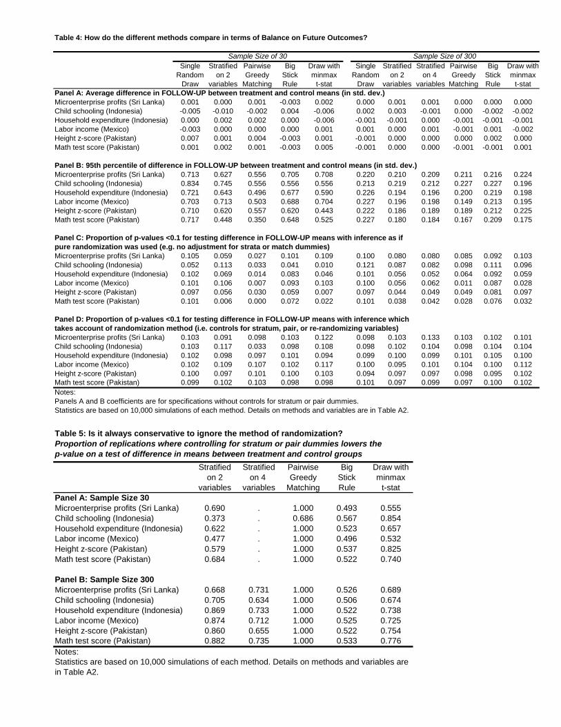
Table 4: How do the different methods compare in terms of Balance on Future Outcomes?

Single Stratified Pairwise Big Draw with Single Stratified Stratified Pairwise Big Draw withRandom on 2 Greedy Stick minmax Random on 2 on 4 Greedy Stick minmax

Draw variables Matching Rule t-stat Draw variables variables Matching Rule t-statPanel A: Average difference in FOLLOW-UP between treatment and control means (in std. dev.)Microenterprise profits (Sri Lanka) 0.001 0.000 0.001 -0.003 0.002 0.000 0.001 0.001 0.000 0.000 0.000Child schooling (Indonesia) -0.005 -0.010 -0.002 0.004 -0.006 0.002 0.003 -0.001 0.000 -0.002 -0.002Household expenditure (Indonesia) 0.000 0.002 0.002 0.000 -0.006 -0.001 -0.001 0.000 -0.001 -0.001 -0.001Labor income (Mexico) -0.003 0.000 0.000 0.000 0.001 0.001 0.000 0.001 -0.001 0.001 -0.002Height z-score (Pakistan) 0.007 0.001 0.004 -0.003 0.001 -0.001 0.000 0.000 0.000 0.002 0.000Math test score (Pakistan) 0.001 0.002 0.001 -0.003 0.005 -0.001 0.000 0.000 -0.001 -0.001 0.001

Panel B: 95th percentile of difference in FOLLOW-UP between treatment and control means (in std. dev.)Microenterprise profits (Sri Lanka) 0.713 0.627 0.556 0.705 0.708 0.220 0.210 0.209 0.211 0.216 0.224Child schooling (Indonesia) 0.834 0.745 0.556 0.556 0.556 0.213 0.219 0.212 0.227 0.227 0.196Household expenditure (Indonesia) 0.721 0.643 0.496 0.677 0.590 0.226 0.194 0.196 0.200 0.219 0.198Labor income (Mexico) 0.703 0.713 0.503 0.688 0.704 0.227 0.196 0.198 0.149 0.213 0.195Height z-score (Pakistan) 0.710 0.620 0.557 0.620 0.443 0.222 0.186 0.189 0.189 0.212 0.225Math test score (Pakistan) 0.717 0.448 0.350 0.648 0.525 0.227 0.180 0.184 0.167 0.209 0.175

Panel C: Proportion of p-values <0.1 for testing difference in FOLLOW-UP means with inference as ifpure randomization was used (e.g. no adjustment for strata or match dummies)Microenterprise profits (Sri Lanka) 0.105 0.059 0.027 0.101 0.109 0.100 0.080 0.080 0.085 0.092 0.103Child schooling (Indonesia) 0.052 0.113 0.033 0.041 0.010 0.121 0.087 0.082 0.098 0.111 0.096Household expenditure (Indonesia) 0.102 0.069 0.014 0.083 0.046 0.101 0.056 0.052 0.064 0.092 0.059Labor income (Mexico) 0.101 0.106 0.007 0.093 0.103 0.100 0.056 0.062 0.011 0.087 0.028Height z-score (Pakistan) 0.097 0.056 0.030 0.059 0.007 0.097 0.044 0.049 0.049 0.081 0.097Math test score (Pakistan) 0.101 0.006 0.000 0.072 0.022 0.101 0.038 0.042 0.028 0.076 0.032

Panel D: Proportion of p-values <0.1 for testing difference in FOLLOW-UP means with inference whichtakes account of randomization method (i.e. controls for stratum, pair, or re-randomizing variables)Microenterprise profits (Sri Lanka) 0.103 0.091 0.098 0.103 0.122 0.098 0.103 0.133 0.103 0.102 0.101Child schooling (Indonesia) 0.103 0.117 0.033 0.098 0.108 0.098 0.102 0.104 0.098 0.104 0.104Household expenditure (Indonesia) 0.102 0.098 0.097 0.101 0.094 0.099 0.100 0.099 0.101 0.105 0.100Labor income (Mexico) 0.102 0.109 0.107 0.102 0.117 0.100 0.095 0.101 0.104 0.100 0.112Height z-score (Pakistan) 0.100 0.097 0.101 0.100 0.103 0.094 0.097 0.097 0.098 0.095 0.102Math test score (Pakistan) 0.099 0.102 0.103 0.098 0.098 0.101 0.097 0.099 0.097 0.100 0.102Notes:Panels A and B coefficients are for specifications without controls for stratum or pair dummies. Statistics are based on 10,000 simulations of each method. Details on methods and variables are in Table A2.

Sample Size of 30 Sample Size of 300

Table 5: Is it always conservative to ignore the method of randomization?Proportion of replications where controlling for stratum or pair dummies lowers the p-value on a test of difference in means between treatment and control groups

Stratified Stratified Pairwise Big Draw withon 2 on 4 Greedy Stick minmax

variables variables Matching Rule t-statPanel A: Sample Size 30Microenterprise profits (Sri Lanka) 0.690 . 1.000 0.493 0.555Child schooling (Indonesia) 0.373 . 0.686 0.567 0.854Household expenditure (Indonesia) 0.622 . 1.000 0.523 0.657Labor income (Mexico) 0.477 . 1.000 0.496 0.532Height z-score (Pakistan) 0.579 . 1.000 0.537 0.825Math test score (Pakistan) 0.684 . 1.000 0.522 0.740

Panel B: Sample Size 300Microenterprise profits (Sri Lanka) 0.668 0.731 1.000 0.526 0.689Child schooling (Indonesia) 0.705 0.634 1.000 0.506 0.674Household expenditure (Indonesia) 0.869 0.733 1.000 0.522 0.738Labor income (Mexico) 0.874 0.712 1.000 0.525 0.725Height z-score (Pakistan) 0.860 0.655 1.000 0.522 0.754Math test score (Pakistan) 0.882 0.735 1.000 0.533 0.776Notes:Statistics are based on 10,000 simulations of each method. Details on methods and variables are in Table A2.

Table 6: How do the different methods compare in terms of Power in detecting a given treatment effect?

Single Stratified Pairwise Big Draw with Stratified Matching 20Random on 2 Greedy Stick minmax on on strata

Draw variables Matching Rule t-stat i.i.d noise i.i.d. noise i.i.d. noisePanel A: Proportion of p-values<0.10 when no adjustment is made for method of randomizationMicroenterprise profits (Sri Lanka) 0.144 0.106 0.095 0.139 0.154 0.132 0.086 0.111Child schooling (Indonesia) 0.123 0.146 0.111 0.115 0.066 0.116 0.144 0.119Household expenditure (Indonesia) 0.390 0.382 0.342 0.382 0.360 0.388 0.387 0.391Labor income (Mexico) 0.181 0.177 0.098 0.178 0.184 0.177 0.203 0.208Height z-score (Pakistan) 0.174 0.134 0.133 0.134 0.052 0.195 0.194 0.193Math test score (Pakistan) 0.167 0.051 0.016 0.139 0.087 0.154 0.131 0.193

Panel B: Proportion of p-values<0.10 when adjustment is made for randomization method(and for the single random draw controls for the seven baseline variables are added to the regression)Microenterprise profits (Sri Lanka) 0.130 0.135 0.153 0.131 0.167 0.144 0.164 0.109Child schooling (Indonesia) 0.109 0.131 0.121 0.112 0.095 0.118 0.144 0.149Household expenditure (Indonesia) 0.409 0.424 0.580 0.419 0.461 0.387 0.356 0.280Labor income (Mexico) 0.164 0.172 0.242 0.167 0.196 0.165 0.173 0.125Height z-score (Pakistan) 0.246 0.201 0.206 0.251 0.281 0.161 0.157 0.142Math test score (Pakistan) 0.183 0.313 0.320 0.187 0.217 0.159 0.170 0.129

Single Stratified Stratified Pairwise Big Draw with Stratified Matching 200Random on 2 on 4 Greedy Stick minmax on on strata

Draw variables variables Matching Rule t-stat i.i.d noise i.i.d. noise i.i.d. noisePanel C: Proportion of p-values<0.10 when no adjustment is made for method of randomizationMicroenterprise profits (Sri Lanka) 0.288 0.274 0.278 0.267 0.280 0.280 0.285 0.279 0.278Child schooling (Indonesia) 0.606 0.585 0.562 0.607 0.597 0.600 0.560 0.610 0.555Household expenditure (Indonesia) 0.999 0.999 1.000 1.000 0.999 1.000 0.999 0.999 0.999Labor income (Mexico) 0.494 0.486 0.480 0.475 0.489 0.474 0.479 0.484 0.489Height z-score (Pakistan) 0.728 0.757 0.756 0.766 0.743 0.767 0.727 0.728 0.739Math test score (Pakistan) 0.615 0.654 0.650 0.655 0.619 0.657 0.631 0.624 0.620

Panel D: Proportion of p-values<0.10 when adjustment is made for randomization method(and for the single random draw controls for the seven baseline variables are added to the regression)Microenterprise profits (Sri Lanka) 0.301 0.305 0.343 0.290 0.302 0.309 0.283 0.338 0.295Child schooling (Indonesia) 0.608 0.596 0.589 0.602 0.600 0.595 0.458 0.607 0.403Household expenditure (Indonesia) 1.000 1.000 1.000 1.000 1.000 1.000 0.999 0.998 0.994Labor income (Mexico) 0.584 0.561 0.541 0.761 0.584 0.582 0.501 0.602 0.408Height z-score (Pakistan) 0.863 0.849 0.854 0.853 0.867 0.866 0.741 0.721 0.642Math test score (Pakistan) 0.812 0.792 0.781 0.829 0.816 0.826 0.630 0.603 0.460Notes:Statistics are based on 10,000 simulations of each method. Details on methods and variables are in Table A2.Stratifications on i.i.d noise are for 8 (48) strata in the sample of 30 (300) observations.Simulated treatment effects are as follows

Child schooling: One in three randomly selected children in the treatment group who would have dropped out don't

Labor income: A 920 Peso increase in income (about 20% of average baseline income)

Sample Size of 30

Math test score: An increase of one quarter of a standard deviation in the test score

Height z-score: An increase of one quarter of a standard deviation in the z-score, where the z-score is defined as standard deviations from mean US height for age

Microenterprise profits: A 1,000 Sri Lankan Rupee increase in profits (about 25% of average baseline profits)

Household expenditure: An increase of 0.4 in ln household expenditure per capita, which corresponds to about one half a standard deviation or moving a household from the 25th to the 50th percentile.

Sample Size of 300

Table 7: How does stratification vary with the number of strata?Simulation results

Stratified Stratified Stratified Stratified Stratified Stratifiedon 2 on 3 on 4 on 2 on 3 on 4

variables variables variables variables variables variables(8 strata) (24 strata) (48 strata) (8 strata) (24 strata) (48 strata)

Panel A: Imbalance - 95th percentile of difference in follow-up meansMicroenterprise profits (Sri Lanka) 0.322 0.338 0.338 0.210 0.213 0.209Child schooling (Indonesia) 0.399 0.346 0.369 0.219 0.211 0.212Household expenditure (Indonesia) 0.337 0.335 0.343 0.194 0.193 0.191Labor income (Mexico) 0.335 0.327 0.344 0.196 0.196 0.198Height z-score (Pakistan) 0.297 0.299 0.310 0.186 0.191 0.189Math test score (Pakistan) 0.285 0.298 0.316 0.180 0.181 0.184

Panel B: Power: Proportion of p-values<0.10 when no strata dummies includedMicroenterprise profits (Sri Lanka) 0.129 0.138 0.144 0.274 0.281 0.278Child schooling (Indonesia) 0.303 0.267 0.273 0.585 0.574 0.562Household expenditure (Indonesia) 0.852 0.850 0.845 0.999 1.000 1.000Labor income (Mexico) 0.170 0.161 0.180 0.486 0.486 0.480Height z-score (Pakistan) 0.286 0.295 0.297 0.757 0.757 0.756Math test score (Pakistan) 0.236 0.245 0.254 0.654 0.649 0.650

Panel C: Power: Proportion of p-values<0.10 when strata dummies includedMicroenterprise profits (Sri Lanka) 0.186 0.273 0.242 0.305 0.327 0.343Child schooling (Indonesia) 0.278 0.301 0.255 0.596 0.596 0.589Household expenditure (Indonesia) 0.904 0.914 0.876 1.000 1.000 1.000Labor income (Mexico) 0.204 0.212 0.199 0.561 0.551 0.541Height z-score (Pakistan) 0.487 0.463 0.457 0.849 0.843 0.854Math test score (Pakistan) 0.464 0.464 0.399 0.792 0.790 0.781Notes:Statistics are based on 10,000 simulations of each method. Details on methods and variables are in Table A2.

Sample Size 100 Sample Size 300