In various ways, the end product of technology is the construction of devicesto perform tasks of varying degrees of sophistication. Such devices range from thedomestic (such as household appliances including cooking aids, washing machines,radios and televisions) to the industrial (such as mechanical machinery includingcranes and tractors; fabrication aids including lathes and drills; and fabricationmachinery such as spinning and weaving devices for cloth making), and on tothe advanced technological (such as the bionic ear, radar, robots and medicalscanners). The majority of such devices contain moving parts often powered byelectric motors. For obvious engineering reasons, such products are classified aselectro-mechanical devices.

Though electromechanical devices can be designed to perform specific tasksexactly, the actual products will only perform the tasks with error, because man-ufacture can only reproduce designs approximately. As this error is usually (andcan even be designed to be) of lower amplitude and of higher frequency than thetask being accomplished, it is often referred to as jitter.

For many devices, such as household appliances like mixers, cleaners and wash-ing machines, simple engineering design criteria can ensure that the jitter is vir-tually non-existent to the user and casual observer, except for some backgroundnoise and minor vibration at high operational speeds. Here, jitter itself is not apotential source for degrading the operational performance of the product. Formore advanced technological devices such as robots and medical scanners, the sit-uation changes. Interaction between the individual (local) jitters, produced by thevarious components of a complex system, such as a robot arm, can produce anaccumulated (global) jitter which degrades performance and is difficult to modeland predict. Now, it is not simply a matter of designing (with respect to given en-gineering criteria) a device to perform exactly some specific task; but of modellingthe tolerances in the manufacturing process so that the jitter in the actual productcan be predicted and thereby controlled.

In an industrial mathematics context, we have a situation where mathematicalexpertise is sought because the standard (engineering) approaches have failed. Itis natural to first seek to control the degradation in the performance of a productwithin the framework in which it is designed. It is only necessary to move into amore sophisticated framework when it is clear that the original one is deficient insome fundamental way.

This characterises the situation facing Ausonics. They manufacture ultrasonicbody scanners (Figure 1). Each one consists of a light and robust hand-held probe(which can be placed on any part of the body) connected by a long flexible lead toa compact and semi-portable unit containing all the electronics (including powersources, controls and small TV-monitor) which do not need to be located in theprobe. The probe itself is the electromechanical device. Because the underlyingtechnology is ultrasonic radar imaging (echography), the scanner is able to operatein real-time to give local cross-sectional pictures (on the TV-monitor) of the bodydirectly below and in the plane scanned by the probe (Figure 2). Their utility as areal-time diagnostic medical aid is therefore clear. In fact, Ausonics already havean established international market.

The problem for Ausonics is that, though they make many probes with vir-tually no jitter, they also produce in the process a large number of probes withunacceptable jitter. For the user, this jitter manifests itself as high frequency small

UL TRASONIC ECHOGRAPHY

Transmittedpulse

t ransm iss ionpulse

direct ion

Figure 2: Diagrarnrnatics of probe imaging.

Received(Return)

pulse

I ntenModul

disp

amplitude movement of the image displayed on the TV-monitor which should notbe there. The seriousness of the problem is reflected in the fact that the cost ofmanufacturing of a probe (because of its moving parts) is a major component inthe price of a scanner, and, on occasions, up to one third of the probes are rejectedbecause of unacceptable jitter.

For this problem, the goal of the Study Group became the modelling and anal-ysis of the electro-mechanical mechanism inside the probe. Even though the elec-tronic processing in the unit, of the signal transmitted from the probe, also pro-duces jitter (in the image displayed on the TV-monitor), it was assessed to be ofsecondary importance at this stage, and was therefore not studied.

The jitter in the Ausonics scanner manifests itself as a high frequency smallamplitude movement of the image displayed on the TV-monitor, which should notbe there. It is different from the low frequency movement within the image record-ing the dynamics of the object being probed, and must therefore be characterisedaccordingly. Thus, jitter is error, which is more complex than is characterisableusing the usual statistical models. Compared with observational errors, which aremodelled assuming the positions of the image pixels remain fixed in time, jittermust be characterised, modelled and analysed in terms of the changing positionsof the image pixels as a function of time.

A corresponding situation arises when we watch a movie. Normally, we onlysee the movement which the image itself represents. Ignoring flickering in thelight source, jitter occurs when the position of the image on the screen changesfrom frame to frame due to a malfunctioning in the projection equipment (whichincludes the film). This also highlights the fact that the movement of the image isnot the origin of the jitter (in the scanner or movie), but its manifestation.

Just as for the movie, where one eliminates the jitter by correcting the malfunc-tion in the projection equipment, the jitter in the scanner can only be eliminatedby correctly identifying and analysing the source in the scanner of the movementin the positions of the image pixels. This is the basis for the goal articulated in theIntrod uction.

Independent justification for identifying and analysing the source in the scannerof the movement arises because jitter in the image cannot be removed by standardfiltering techniques. In fact, a moment's reflection indicates that

Frame 2(error/no jitter)

Frame 2(jitter/no error)

Figure 3: Effect of smoothing (averaging) on successive jittered and non-jittered-c _

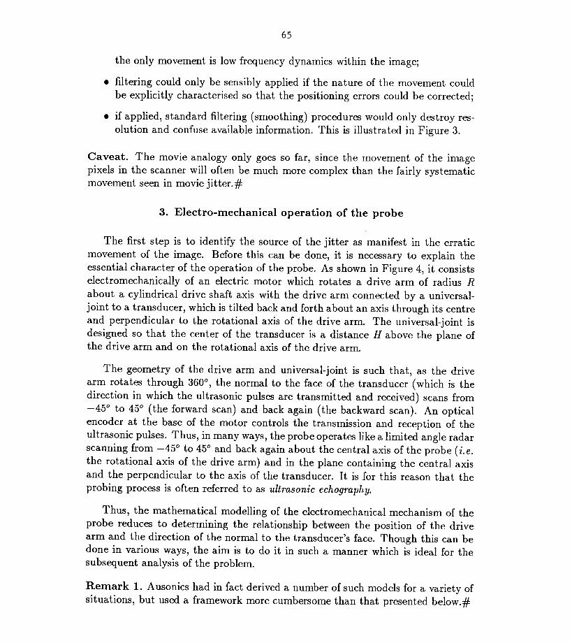
the only movement is low frequency dynamics within the image;

• filtering could only be sensibly applied if the nature of the movement couldbe explicitly characterised so that the positioning errors could be corrected;

• if applied, standard filtering (smoothing) procedures would only destroy res-olution and confuse available information. This is illustrated in Figure 3.

Caveat. The movie analogy only goes so far, since the movement of the imagepixels in the scanner will often be much more complex than the fairly systematicmovement seen in movie jitter.#

The first step is to identify the source of the jitter as manifest in the erraticmovement of the image. Before this can be done, it is necessary to explain theessential character of the operation of the probe. As shown in Figure 4, it consistselectromechanically of an electric motor which rotates a drive arm of radius Rabout a cylindrical drive shaft axis with the drive arm connected by a universal-joint to a transducer, which is tilted back and forth about an axis through its centreand perpendicular to the rotational axis of the drive arm. The universal-joint isdesigned so that the center of the transducer is a distance H above the plane ofthe drive arm and on the rotational axis of the drive arm.

The geometry of the drive arm and universal-joint is such that, as the drivearm rotates through 360°, the normal to the face of the transducer (which is thedirection in which the ultrasonic pulses are transmitted and received) scans from-45° to 45° (the forward scan) and back again (the backward scan). An opticalencoder at the base of the motor controls the transmission and reception of theultrasonic pulses. Thus, in many ways, the probe operates like a limited angle radarscanning from -45° to 45° and back again about the central axis of the probe (i.e.the rotational axis of the drive arm) and in the plane containing the central axisand the perpendicular to the axis of the transducer. It is for this reason that theprobing process is often referred to as ultrasonic echography.

Thus, the mathematical modelling of the electromechanical mechanism of theprobe reduces to determining the relationship between the position of the drivearm and the direction of the normal to the transducer's face. Though this can bedone in various ways, the aim is to do it in such a manner which is ideal for thesubsequent analysis of the problem.

Remark 1. Ausonics had in fact derived a number of such models for a variety ofsituations, but used a framework more cumbersome than that presented below.#

H HEIGHT OF CENTERI ;F TRANSDUCER ABOVE.\( DRIVE PLANE

~ 0ADIUS OFDRIVE ARM

CIRCULAR PATH OFDRIVE POINT

.~

RANSDUCERANGLE(9) tan 9 • cos a.

'\.

"PLANE OF

SCAN

FOR TRANSDUCER

ANGLE a

PLANE OF

DRIVE ARM

rj-R.rR

I

II

I

CURRENT POSITION

OF DRIVE ARM

TRANSDUCERAXIS

TH1-

BECAUSE OFAXIAL SYMMETRY

NO END VIEW

REQUIRED

POLAR COORDINATEAXIS FOR ANGLE

OF DRIVE ARM ex

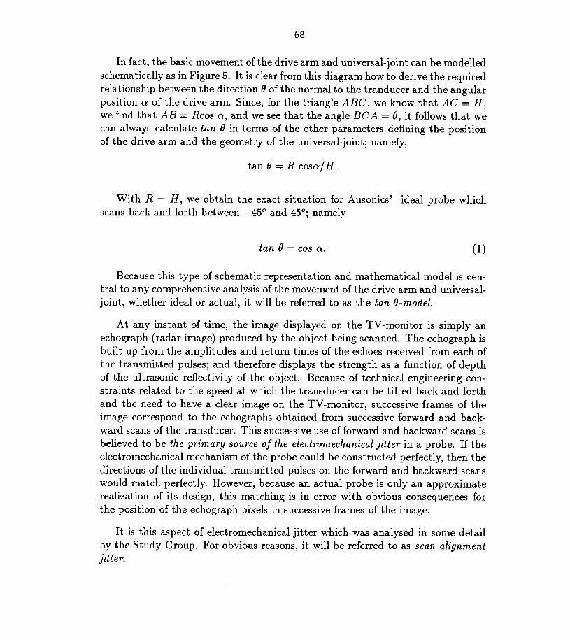
In fact, the basic movement of the drive arm and universal-joint can be modelledschematically as in Figure 5. It is clear from this diagram how to derive the requiredrelationship between the direction 0 of the normal to the tranducer and the angularposition a of the drive arm. Since, for the triangle ABC, we know that AC = H,we find that AB = Rcos a, and we see that the angle BCA = 0, it follows that wecan always calculate tan 0 in terms of the other parameters defining the positionof the drive arm and the geometry of the universal-joint; namely,

With R = H, we obtain the exact situation for Ausonics' ideal probe whichscans back and forth between -45° and 45°; namely

Because this type of schematic representation and mathematical model is cen-tral to any comprehensive analysis of the movement of the drive arm and universal-joint, whether ideal or actual, it will be referred to as the tan O-model.

At any instant of time, the image displayed on the TV-monitor is simply anechograph (radar image) produced by the object being scanned. The echograph isbuilt up from the amplitudes and return times of the echoes received from each ofthe transmitted pulses; and therefore displays the strength as a function of depthof the ultrasonic reflectivity of the object. Because of technical engineering con-straints related to the speed at which the transducer can be tilted back and forthand the need to have a clear image on the TV-monitor, successive frames of theimage correspond to the echographs obtained from successive forward and back-ward scans of the transducer. This successive use of forward and backward scans isbelieved to be the primary source of the electromechanical jitter in a probe. If theelectromechanical mechanism of the probe could be constructed perfectly, then thedirections of the individual transmitted pulses on the forward and backward scanswould match perfectly. However, because an actual probe is only an approximaterealization of its design, this matching is in error with obvious consequences forthe position of the echograph pixels in successive frames of the image.

It is this aspect of electromechanical jitter which was analysed in some detailby the Study Group. For obvious reasons, it will be referred to as scan alignmentjitter.

IDEAL DESIGNALIGNMENT

FORWARD BACKSCAN SCAN

::. -- -- -...,

- --~ -

•......••1J...

IDEAL •tan e - CURVE -

....•....\

••• ACTUAL•••• tan e -CURVE

•••• EXAGGERA TED..•••

FORWARD -------_-!-4----SCAN I BACK

SCAN

ACTUAL DESIGNALIGNMENT

FORWARD BACKSCAN SCAN

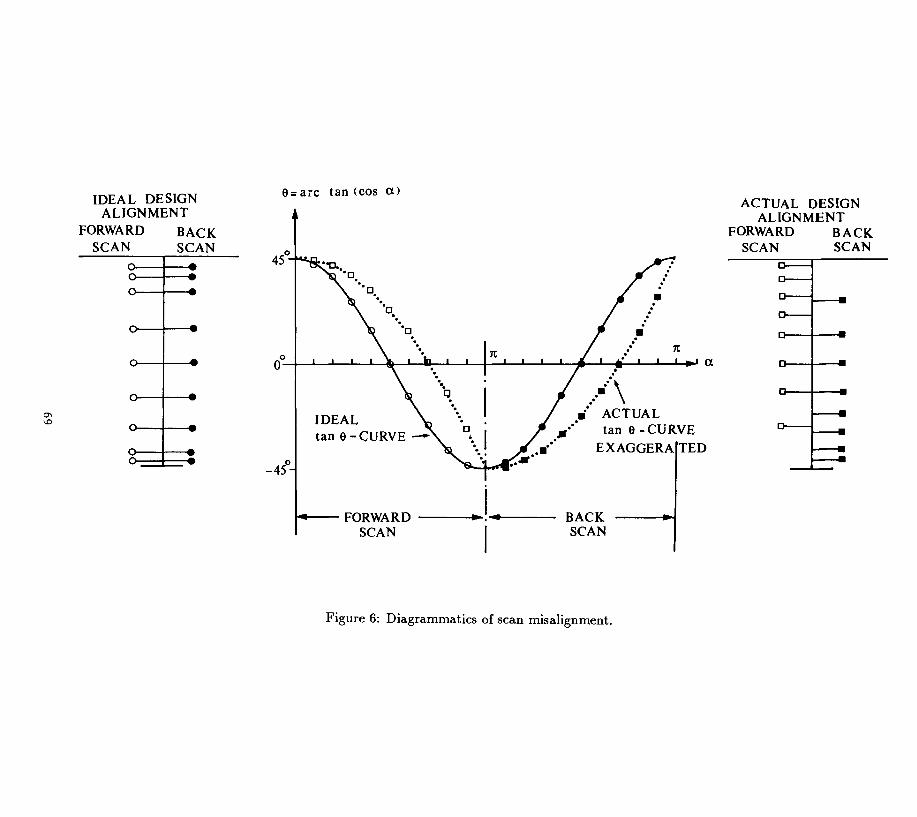
Mathematically, the study of scan alignment jitter reduces to quantifying themisalignment between forward and back scans in terms of the errors which arise inconstructing an actual probe (when compared with its ideal design). The crucialrole of the tan O-model in quantifying such misalignment is illustrated in Figure 6.In order to interpret it, we first note that the time between successive transmissionsof the ultrasonic pulses is held constant. This is achieved by coupling the opticalencoder to the rotation of the drive shaft since it moves with constant angularvelocity. Thus, for the interpretation of Figure 6, we assume that the transmissions(and hence the recording of the return pulses) occur at equal steps along the a-axis.

For the ideal design, we see immediately from Figure 6 that misalignment iszero because of the symmetry about a = 180° of the ideal tan O-curve (which isthe graphical realization of the algebraic formula (1)). The severity of the mis-alignment which can occur is also illustrated for an actual tan O-curve which hasbeen distorted from the ideal (including symmetry about a = 180°) by the errorsin the construction of the actual probe it represents.

The goal set by Ausonics was not to explicitly quantify the nature of the mis-alignment so that it can be partially corrected at some subsequent stage (e.g.electronically in the unit); but to identify the construction errors which contributethe most to the misalignment so that appropriate quality control can be introducedat the production stage. Thus, from the point of view of the present investigation,the examination of scan alignment jitter reduced to deriving and analysing tan 0-models for various configurations of actual probes (in how they differ from the idealdesign).

The construction of such tan O-models is always possible, because, as the tophalf of Figure 5 illustrates, a pulse transmission direction will always be relatableto a triangle ABC which characterises the current position of the drive arm (as afunction of the drive angle a and the errors in the construction) to the effectiveheight of the origin C of the transmission directions above the plane of rotation ofthe drive arm.

In this Section, we identify and discuss some of the possible design errors (i. e.the ways in which an actual probe can differ from its ideal design) as well as listfor each the relevant tan O-model. They are easily derived by generalising theargument built around Figure 5 which was used above to derive the tan O-model

II---+r FRONT VIEW

I H

1I

-1- --TILT OF

DRIVE ARMPLANE

AII II I

~~IR sina tan'Y../ I

I

I

10+-- H--

for the ideal design. Finally, for what is surmised to be a highly relevant tan 0-model, we make a detailed error analysis and give our interpretation of the resultsas they apply to Ausonics' situation.

When constructing an actual probe, some possible design errors which can occurare:

1. Slap (slack) slop) in drive arm and transducer mountings

Because the probe is a dynamic (not a static) mechanism, and because thejoining of components is not completely rigid, the tilting of the transducermay not be directly coupled to the movement of the drive arm. The appro-priate tan O-model is

where 1J denotes the transducer angle relevant to this situation, lie the tilt-slap in the transducer mounting, and liOt the rotational-slap in the drive armmounting. This tan O-model can also be used to account for the situationwhere the a-axis is not perpendicular to the axis of tilt of the transducer.

Remark 2. We express all tan O-models in terms of the same drive armangle a, since it is the position of the drive arm which determines the tiltof the transducer. This easily allows for the incorporation of errors in theoptical encoder, since these errors will only affect the points along the a-axisat which the ultrasonic pulses are transmitted.#

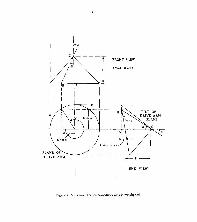
2. Misalignment of transducer axisThrough errors in the construction of the universal-joint, the axis of thetransducer may not be parallel to the drive arm plane. By considering theequivalent situation where the drive arm plane is tilted relative to the trans-ducer axis, the corresponding tan O-model is found to be (Figure 7)

tan {) = R cosa / (H + R sina tan,)

where {)denotes the transducer angle relevant to this situation, and, theangle the transducer axis makes with the drive arm plane. Without loss ofgenerality and in order to simplify the form of the right hand side of (3), ,was chosen as shown in Figure 7.

Remark 3. Though Ausonics had previously obtained a version of thisformula, it was more complex than (3), even though it assumed that R = H.The simplicity of (3) results from the way we have defined " and the explicitimplementation of the tan O-modelling formalised above.#

r PLANE OFSCAN

PLANE OF

DRIVE ARM

3. Positioning of centre of transducer above drive arm planeBecause of the complex structure of the probe from a manufacturing pointof view, it will be difficult to ensure that the centre of the transducer is(a) exactly a distance R above the drive arm plane; and(b) on the drive arm axis.

tan 0 = R cosa/ H,

where 0 denotes the transducer angle relevant to the situation identified in(a); and

tan 0 = (R cosa + .6. cos<!J)/H

where 0 denotes the transducer angle relevant to the situation identified in(b), and .6. and <!Jdefine the offset between the centre of the transducer andthe axis of the drive arm as shown in Figure 8.

Remark 4. In all the formulas derived by Ausonics, it was assumed that R = H.The consequences of this will be pursued below. #

Thus, the general design error situation is characterised by a misaligned trans-ducer axis and a poorly positioned transducer. It follows from (3) and (5) andtheir derivations that the general tan O-model is given by

As mentioned above, from Ausonics' point of view, the goal is to determinewhich design errors (in terms of a, R, H, 8, <p and ,) affect most the alignmentbetween the transmission directions on the forward and back scans. In part, theproblem thereby reduces, for a given tan O-model, to analysing the effect on thecorresponding transducer angle of perturbations in the design variables, whichcorresponds to a classical error analysis. Since a comprehensive account of suchdeliberations is beyond the scope of this Report, we briefly sketch such an analysisand discuss the resulting interpretations for a simple (but important) situation notpreviously considered by Ausonics; namely, the tan O-model of equation (4) whereH is assumed to depend on a. An examination of the construction of the probeindicates that the drive arm is a single solid component of fixed length R whereasthe height H of the centre of the transducer above the drive arm plane dependson the construction and movement of the universal joint in which the transducer

is mounted. It is therefore natural to assume that R is fixed (independent of 0:),and that H depends on 0: and, up to first order, equals R.

- RH dHdO = - ( 2 R2 2) (sino: do:+ coso: H ),H + cos 0:

smo: do:1 + cos20:

coso: dH1 + cos20: H

smo: d---- 0:.1+ cos20:

coso: dHdO -=- dO -1+ cos20: H

Together, equations (7) and (9) give a detailed picture of the effect of H, whencompared with the ideal situation characte~ised by (8). In fact, we can draw thefollowing conclusions:

(a) For the ideal design, it follows from (8) that the transducer angle is mostsensitive to perturbations in 0: when 0: f"V 11"/2 and 311"/2 and least sensitive when0: f"V 0 and 11". From a design point of view, this has good and bad aspects. Since,when examining an image on the TV-monitor, the eye seeks information from thecentral (rather than peripheral) region of the picture, this is bad as the aboveinterpretation implies that, for errors in the optical encoder, jitter will be worstin the central region of the image. It is good in the sense that encoder inducedjitter will be least where slap in the drive arm and transducer mountings couldhave most effect.

(b) From (9) it follows that the effect of H is to introduce an additive errorinto the ideal situation.

(c) Equation (7) shows that the effect of H will be out of phase with encoderinduced errors in the ideal situation. Thus, its jitter will be less crucial in thecentral region of the image.

(d) From a manufacturing point of view, the most disturbing aspect about thestructure of the additive error due to H is that it is a relative error term, sincein construction tolerances are specified as absolute errors (which we know do notnecessarily control relative errors).

Acknowledging that other aspects would have to be examined in a more com-prehensive investigation of the electronic and electro-mechanical jitter in Ausonics'scanner, the Study Group concentrated attention on what was believed to be a pri-mary source of the jitter; namely, scan alignment jitter. As outlined in the Reportabove, the Study Group made considerable progress with the modelling, analy-sis and interpretation of this source, and thereby laid a basis for a more detailedinvestigation of scan alignment jitter. In particular, the Study Group

• formulated a quite simple procedure for determining tan O-models and thenderived them for a variety of design errors;

• gave an error analysis for a simple (but important) situation not previouslyconsidered by Ausonics; and, thereby,

• derived conclusions about the scan alignment jitter not previously appreci-ated by Ausonics.

The moderator would first like to thank Ausonics and their Project Manager,Dr. Jim Rathmell, for the support such as displays, information, briefings, etc.given to the Study Group throughout its deliberations; and second to acknowledgethe enthusiastic assistance of the participants who devoted a major portion of theirtime to the investigation of this Problem (namely, Chris Harman, Lyle Noakes,Mike O'Neill, Phil Sheridan, Noel Thompson, Peter Trudinger and Kevin Wilkins).