In Copyright - Non-Commercial Use Permitted Rights ...1817/eth... · Tessaro, Stefano M. ......
216
Research Collection Doctoral Thesis Computational Indistinguishability Amplification Author(s): Tessaro, Stefano M. Publication Date: 2010 Permanent Link: https://doi.org/10.3929/ethz-a-006183893 Rights / License: In Copyright - Non-Commercial Use Permitted This page was generated automatically upon download from the ETH Zurich Research Collection . For more information please consult the Terms of use . ETH Library
Transcript of In Copyright - Non-Commercial Use Permitted Rights ...1817/eth... · Tessaro, Stefano M. ......

Research Collection
Doctoral Thesis
Computational Indistinguishability Amplification
Author(s): Tessaro, Stefano M.
Publication Date: 2010
Permanent Link: https://doi.org/10.3929/ethz-a-006183893
Rights / License: In Copyright - Non-Commercial Use Permitted
This page was generated automatically upon download from the ETH Zurich Research Collection. For moreinformation please consult the Terms of use.
ETH Library
Diss. ETH No. 19204
Computational IndistinguishabilityAmplification
A dissertation submitted to
ETH ZURICH
for the degree ofDoctor of Sciences
presented by
Stefano TessaroMSc ETH CS, ETH Zurich
born July 4, 1981citizen of Coldrerio, TI, Switzerland
accepted on the recommendation of
Prof. Dr. Ueli Maurer, examinerProf. Dr. Thomas Holenstein, co-examiner
Prof. Dr. Salil Vadhan, co-examiner
2010

ii

iii
Acknowledgments
First of all, I would like to thank my advisor, Ueli Maurer. His door hasalways been open, not only for research discussions, but also every singletime I have been in need of any kind of advice. I have learned a lot fromhim: Most of the questions addressed within this thesis are motivated bythe abstract viewpoint on cryptography Ueli has been advocating overthe years, and which has had a substantial impact on my approach toresearch.
Moreover, I am deeply grateful to both Thomas Holenstein and SalilVadhan for serving on my committee, for reviewing my thesis, and fortheir valuable feedback. In particular, Thomas is responsible to a non-negligible extent for my interest in complexity-theoretic cryptographythat I developed in an earlier stage of my graduate studies.
Of course, my time at ETH would have been far less pleasant with-out all the great colleagues with whom I have shared so many discus-sions about research, life, the universe, and everything (as well as count-less foosball matches...): This includes Divesh Aggarwal, Joel Alwen,Georges Baatz, Kfir Barhum, Zuzana Beerliova-Trubıniova, David Bern-hard, Sandro Coretti, Chandan Dubey, Matthias Fitzi, Ghislain Fourny,Viktor Gaillard, Peter Gazi, Esther Hanggi, Martin Hirt, Robert Konig,Robin Kunzler, Christoph Lucas, Jun Muramatsu, Krzysztof Pietrzak,Bartosz Przydatek, Dominik Raub, Renato Renner, Junji Shikata, JohanSjodin, Bjorn Tackmann, Douglas Wikstrom, Stefan Wolf, Jurg Wullschle-ger, Vassilis Zikas, and many others I probably forgot to mention.
I am particularly grateful to Peter for inspiring research discussionsthat have led to some of the results of this thesis. Special thanks also goto Vassilis for having been a great friend within the group, and, togetherwith Dominik, Johan, and Sandro, for having been my office mate. Inaddition, I thank our secretary, Beate Bernhard, for her tireless adminis-trative support.
Finally, I am indebted to my parents, Claudio and Marilena, for theircontinuous support, and to Roska, for her love, and for always being onmy side. Without their help and encouragement, I would probably havebeen far from achieving all of this... Grazie di cuore!
The research in this thesis was carried out under partial support fromthe Swiss National Science Foundation (SNF).

iv

v
Abstract
Computational security of cryptographic schemes is always shown un-der the (unproven) assumption that some underlying primitive is secure.In several important examples, the security of these primitives is definedin terms of computational indistinguishability, the property that two sys-tems, despite possibly being very different, exhibit essentially the samebehavior in the eyes of a computationally bounded observer. The mostprominent example is a pseudorandom generator (PRG), an efficientlycomputable function stretching a short random secret seed into a longerstring which is computationally indistinguishable from an equally longrandom string. Further examples are pseudorandom functions (PRFs)and permutations (PRPs), keyed functions and permutations which, un-der a random secret key, behave as a uniformly chosen function and per-mutation, respectively. Pseudorandom systems underlie essentially allefficient secret-key cryptographic schemes, and are frequent importantcomponents in public-key schemes and cryptographic protocols. Also, itis common to assume that block ciphers, such as the Advanced Encryp-tion Standard (AES), are secure PRPs.
Yet computational indistinguishability is a strong requirement, andcontinuous progress in the development of cryptanalytic techniques castssome doubt as to whether such assumptions are any longer justified forexisting designs. To this end, this dissertation addresses the fundamentalquestion of basing efficient cryptography on primitives satisfying sub-stantially weaker forms of computational indistinguishability. In par-ticular, we refer to computational indistinguishability amplification as theproblem of strengthening such primitives, and consider, throughout thiswork, two main axes along which amplification is achieved.
The first and main part of this thesis addresses the case where the ob-server is allowed to achieve some non-negligible (albeit quantitativelybounded) advantage over random guessing in distinguishing the twosystems. By means of a series of general theorems, we undertake an in-depth investigation of the behavior of the computational distinguishingadvantage under different forms of system composition, with the aim offinding efficient combination operations reducing the computational dis-tinguishing advantage. All these results apply to the general class of sys-tems whose state does not depend on the interaction, which comprisesmost cryptographic systems of interest. Our most important applicationis an exact characterization of the security amplification achieved by thecascade (i.e., sequential composition) of PRPs with respect to the distin-
vi
guishing advantage, a long-standing open problem. (Even stronger am-plification is shown under a minimal modification of the cascade.) Also,we provide a construction for security amplification of weak PRGs withoptimal output length, as well as tighter and / or simpler proofs for allexisting results in the literature in the context of advantage amplification.
A key technique is the generalization of complexity-theoretic results,such as Yao’s XOR Lemma and Impagliazzo’s Hardcore Lemma, to thesetting of interactive systems, which is of independent interest. Also,most of our results can be interpreted as computational analogues ofinformation-theoretic results, and help providing a better understandingof the intrinsic relationship between information-theoretic and computa-tional security.
In contrast, the final part of this thesis is devoted to a weaker formof computational indistinguishability where the observer is only grantedrestricted access to the given system. In particular, we consider PRFswhere computational indistinguishability only holds for observers whichare allowed a bounded number (e.g., a constant as low as two) of ran-dom (but known) queries. We provide constructions of fully secure PRFsfrom such weaker PRFs that even improve on the efficiency of existingconstructions in the literature based on the stronger assumption whereobservers are allowed any number of random queries. Our results yieldefficient encryption schemes from block ciphers, and efficient messageauthentication codes from hash functions, both under such very weakpseudorandomness assumptions on the underlying primitives.

vii
Riassunto
Ogni dimostrazione della sicurezza computazionale di uno schema crit-tografico si basa sull’assunzione, non dimostrata, che una primitiva, imp-iegata come componente, soddisfi a sua volta dei requisiti di sicurez-za computazionale. La sicurezza di tali primitive viene spesso defini-ta tramite il concetto di indistinguibilita computazionale, ossia la proprietasecondo la quale due sistemi crittografici, sebbene sostanzialmente di-versi, presentino un comportamento pressoche identico nei confronti diosservatori la cui potenza di calcolo e limitata. L’esempio piu comunee rappresentato dai cosiddetti generatori pseudocasuali (PRG), funzioni ef-ficienti il cui output, dato un input segreto distribuito uniformemente, ecomputazionalmente indistinguibile da una stringa distribuita uniforme-mente e di lunghezza maggiore dell’input. Ulteriori esempi sono le fun-zioni pseudocasuali (PRF) e le permutazioni pseudocasuali (PRP), funzioni(e rispettivamente permutazioni), indicizzate da una chiave segreta, chesono indistinguibili da una funzione (o permutazione) scelta uniforme-mente dall’insieme di funzioni (o permutazioni) con il medesimo do-minio. I sistemi pseudocasuali sono alla base di quasi tutti gli schemiefficienti in crittografia simmetrica, come pure di molti schemi nella crit-tografia a chiave pubblica e in protocolli crittografici. E inoltre comuneassumere che i cosiddetti block ciphers, come l’Advanced Encryption Stan-dard (AES), sono delle PRP.
L’indistinguibilita computazionale rimane tuttavia una properieta disicurezza molto forte, e i continui progressi nello sviluppo di tecnichecrittanalitiche mettono sempre piu in dubbio la validita dell’assunzioneche l’AES e una PRP. Pertanto, l’obbiettivo primario di questa disser-tazione e uno studio dettagliato di soluzioni crittografiche efficienti basatesu primitive che soddisfano unicamente forme ben piu deboli di indistin-guibilita computazionale. In particolar modo, studieremo il problemadell’amplificazione dell’indistinguibilita computazionale (computationalindistinguishability amplification), ossia il problema di incrementare la si-curezza di queste primitive.
La prima (e maggior) parte di questa tesi si propone di studiare ilcaso dove e permesso all’osservatore, confrontato con il compito di dis-tinguere due sistemi, raggiungere un vantaggio sostanziale (sebbene lim-itato quantitativamente) rispetto a una semplice scelta casuale. Attraver-so una serie di teoremi generali, affronteremo un’analisi quantitativa delcomportamento del vantaggio nel caso di diversi tipi di operazioni dicomposizione di sistemi: l’obbiettivo e di individuare esempi efficienti

viii
di operazioni in grado di ridurre sostanzialmente tale vantaggio. Questirisultati sono applicabili a una classe generale di sistemi con uno sta-to iniziale arbitrario, che non viene pero aggiornato nel corso dell’in-terazione, la quale comprende la maggior parte dei sistemi crittograficid’interesse. L’applicazione principale di questi risultati e una caratter-izzazione esatta dell’amplificazione della sicurezza raggiunta dalla cas-cata (o composizione sequenziale) di PRP, un problema finora irrisolto.Inoltre, una minima modifica della cascata raggiunge un’amplificazioneottimale. Ulteriori applicazioni consistono in un nuovo metodo per incre-mentare la sicurezza di PRG deboli con un output di lunghezza ottimale,come pure analisi semplificate di tutti i risultati precedenti nel contestodell’amplificazione del vantaggio.
Una tecnica chiave nello sviluppo di questi risultati, di interesse in-dipendente, consiste nella generalizzazione al contesto dei sistemi in-terattivi di risultati fondamentali come l’XOR Lemma di Yao e l’HardcoreLemma di Impagliazzo. Inoltre, molti risultati di questa tesi sono interpre-tatabili come analoghi computazionali di teoremi precedentemente di-mostrati nel contesto della sicurezza incondizionata (basata sulla teoriadell’informazione), e contribuiscono pertanto a una migliore compren-sione della relazione fra i due tipi di sicurezza.
La seconda parte della tesi considera un indebolimento dell’indistin-guibilita computazionale attraverso la limitazione dell’accesso. In mo-do particolare, studieremo funzioni pseudocasuali dove all’osservatore eunicamente permessa la valutazione presso un numero limitato (che puoessere addirittura una costante maggiore o uguale a due) di input casuali.Il risultato principale di quest’ultima parte consiste in nuove costruzionidi PRF (per osservatori con valutazioni arbitrarie) da queste varianti diPRF deboli, la cui efficienza e addirittura superiore a quella di preceden-ti costruzioni richiedenti un’assunzione ben piu forte dove il numero divalutazioni a input casuali non e limitato. Due conseguenze dirette sonoun nuovo sistema di cifratura basato su block ciphers, come pure un nuo-vo metodo di autentificazione di messaggi a partire da funzioni di hash,entrambi basati unicamente su tali deboli assunzioni pseudocasuali.

Contents
1 Introduction 11.1 Cryptographic Security . . . . . . . . . . . . . . . . . . . . . 11.2 Cryptographic Assumptions . . . . . . . . . . . . . . . . . . 21.3 Indistinguishability and Pseudorandomness . . . . . . . . 31.4 Computational Indistinguishability Amplification . . . . . 51.5 Outline and Contributions of This Thesis . . . . . . . . . . 6
2 Preliminaries 132.1 Basic Notation . . . . . . . . . . . . . . . . . . . . . . . . . . 132.2 Probabilities and Information-Theoretic Quantities . . . . . 142.3 Discrete Systems . . . . . . . . . . . . . . . . . . . . . . . . 172.4 Indistinguishability of Systems and Game Winning . . . . 242.5 Algorithms and Complexities . . . . . . . . . . . . . . . . . 312.6 Pseudorandom Systems . . . . . . . . . . . . . . . . . . . . 34
3 Weakly Unpredictable Bits 373.1 System-Bit Pairs . . . . . . . . . . . . . . . . . . . . . . . . . 413.2 The Hardcore Lemma for System-Bit Pairs . . . . . . . . . . 443.3 The XOR Lemma for System-Bit Pairs . . . . . . . . . . . . 79
4 Security Amplification for Neutralizing Constructions 954.1 Neutralizing Constructions . . . . . . . . . . . . . . . . . . 974.2 Product Theorem for Neutralizing Constructions . . . . . . 99

x Contents
4.3 Applications of the Product Theorem . . . . . . . . . . . . . 1044.4 A Strong Product Theorem . . . . . . . . . . . . . . . . . . . 1064.5 Applications of the Strong Product Theorem . . . . . . . . 114
5 Security Amplification via Extracting Constructions 1215.1 Hardcore Lemmas for Computational Indistinguishability 1245.2 Extracting Constructions . . . . . . . . . . . . . . . . . . . . 1345.3 Security Amplification for PRGs . . . . . . . . . . . . . . . 1395.4 High-Min-Entropy Function Tables . . . . . . . . . . . . . . 1445.5 Cascade of Weak Permutations . . . . . . . . . . . . . . . . 1495.6 Randomized Cascade and Randomized XOR . . . . . . . . 161
6 From Random-Input to Chosen-Input Indistinguishability 1656.1 The Randomized Cascade Construction . . . . . . . . . . . 1686.2 The Nested Randomized Cascade Construction . . . . . . . 1786.3 Black-Box Keying of Iterated Hash Functions . . . . . . . . 185
7 Concluding Remarks and Open Problems 189
A Additional Technical Material 203A.1 A Technical Lemma on Conditional Expectations . . . . . . 203A.2 Details of the Proof of Theorem 5.3 . . . . . . . . . . . . . . 204

Chapter 1
Introduction
1.1. Cryptographic Security
The primary goal of cryptography can be broadly summarized as the de-sign of schemes that allow a set of honest entities to securely achieve somepre-specified goals in presence an adversary. The most traditional andubiquitous example is the private transmission of information betweentwo parties, Alice and Bob, where an adversary, Eve, eavesdrops theircommunication, this task being usually referred to as message encryption.A further example is message authentication, i.e., the authentic transmis-sion of information in the case where Eve is additionally allowed to tam-per with the communication between Alice and Bob.
Despite wide interests in the deployment of such schemes spanningover two thousand years, only the last decades (starting from the seminalwork of Shannon [Sha49]) have seen cryptography develop itself into ascientific discipline centered around the principle of provable security: Se-curity of cryptographic schemes is formalized in terms of the inability ofan adversary to win a certain game associated with some desired prop-erty of the scheme. The ultimate goal is a security proof, a formal proofthat no adversary is able to win the game.
A central parameter of such security proofs is the computational powergiven to the adversary. The strongest notion (which was considered in

2 Introduction
Shannon’s work) is called information-theoretic (IT) security and requiressecurity for all adversaries, regardless of their computing power. (Theseadversaries are usually called computationally unbounded.) While someprominent tasks, such as message encryption and authentication, enjoysolutions with IT security (granted entities share a private key), the re-sulting schemes are impractical. Even more importantly, a number ofadditional tasks, such as public-key encryption (which is essential for se-cure communication over the Internet, and which has been introduced inthe seminal work of Diffie and Hellman [DH76]), cannot be realized withinformation-theoretic security.
To overcome these limitations, the weaker, yet more realistic, notionof computational security allows secure and efficient realization of a widerrange of functionalities, but only requires the scheme to resist attacksfrom so-called computationally bounded adversaries, i.e., restricted to fea-sible computations: While a computationally secure scheme can, in prin-ciple, always be broken, any successful attack would take an excessiveamount of time (e.g., thousands or even millions of years).
1.2. Cryptographic Assumptions
Information-theoretic security statements are usually unconditional, thatis, their proofs do not rely on any assumptions. In contrast, non-trivialunconditional computational infeasibility proofs remain beyond reach ofknown techniques,1 and computational security is always proven underthe assumption that some simpler cryptographic component (often calleda primitive) is secure or, more generally, that some underlying compu-tational problem is hard. For example, a symmetric encryption schememay rely on a one-way function f : X → Y , an efficiently computable func-tion which is hard to invert,2 or, in the public-key setting, may make useof a group (such as Z∗pq for large primes p and q) where the computationof e-th roots is hard (this is the well-known RSA assumption [RSA78]).
Deployment of provably secure cryptographic schemes thus follows atwo-step approach: First, one identifies a scheme with provable-securityguarantees under a computational assumption on the underlying com-ponent, and second, the underlying component is instantiated (e.g., bymeans of a block cipher, a hash function, or a certain algebraic structure)so that the computational assumption is conjectured to be true.
1Such proofs usually imply P 6= NP .2More specifically, this means that given f(x) for a random secret preimage x, it is com-
putationally hard to find a preimage x′ such that f(x) = f(x′).

1.3 Indistinguishability and Pseudorandomness 3
In general, such conjecture is solely justified by resistance to all cur-rently known attack types, and sudden cryptanalytic breakthroughs mayfalsify it. Consequently, such assumptions need to be as weak as possi-ble: On the one side, it is plausible that designing a primitive satisfyingsuch weaker assumption is a much easier task. On the other side, it is asafe practice to only assume that already existing primitives only satisfymuch weaker security properties than their original design goals.
However, while for example all symmetric cryptographic primitivescan be built based on primitives as weak as one-way functions, the re-sulting constructions are way to inefficient to be any practical use, andthe security losses contained in their security proofs are way too large.We thus experience a trade off between the strength of the assumptionand the efficiency of the scheme relying on it, and the actual problem,in practice, is to find the best compromise between the strength of theassumption and the desired efficiency of the scheme.
1.3. Indistinguishability and Pseudorandomness
Several computational assumptions are formulated in terms of the hard-ness to compute a certain secret, such as the preimage of a one-way func-tion or the e-th root of a group element. Another important class of as-sumptions (and cryptographic primitives), first considered by Blum andMicali [BM82], and which is the object of this thesis, is based on compu-tational indistinguishability, i.e., the property that two systems, which arepossibly completely different, express the same behavior in the eyes of acomputationally bounded observer, usually called a distinguisher.
More in detail, for two interactive systems3 S and T, and for a dis-tinguisher D outputting a decision bit D(F) when interacting with somegiven system F, the distinguishing advantage is defined as
∆D(S,T) := |P [D(S) = 1]− P [D(T) = 1]| ,and, for a set of distinguishers D, we define
∆D(S,T) := supD∈D
∆D(S,T).
Two systems S and T are computationally indistinguishable if ∆E(S,T) is“negligible”, where E is the set of all computationally bounded distin-guishers performing feasible computations.
3We provide a formal definition of such systems below, for now an intuitive understand-ing is sufficient.

4 Introduction
A special case of cryptographic primitives relying on computationalindistinguishability are pseudorandom systems, i.e., systems which onlyuse few random bits as a seed (e.g., from a short secret key) and whichare computationally indistinguishable from an ideal system containingmuch more randomness than the seed. Examples of relevant ideal sys-tems range from a random string longer than the seed (so-called pseu-dorandom generators (PRG) [BM82]) to a randomly chosen function (theseare referred to as pseudorandom functions (PRFs) [GGM84]) and to a ran-domly chosen permutation (pseudorandom permutations (PRPs) [LR86]).Pseudorandom systems underlie essentially all efficient symmetric cryp-tographic schemes,4 and are also central components in a wider context.Also, it is a common assumption that a block cipher, such as the Ad-vanced Encryption Standard (AES), is a PRP under a random secret key.
Building pseudorandom systems appears to be a significantly hardertask than designing primitives with computational hardness guarantees.While in the latter case it suffices to make sure that, with very high prob-ability, some secret is hard to guess, in the former case no efficient distin-guisher must detect any minimal deviation from the behavior of the idealrandom system. However, we do expect simpler constructions of pseu-dorandom primitives if we allow for non-random distribution of theiroutputs. Despite distinguishing from random being much easier, suchprimitives may still ensure the availability of sufficient pseudorandom-ness to be useful in a cryptographic sense.
More concretely, we identify two orthogonal axes along which (com-putational) indistinguishability can be relaxed:
(i) On the one hand, we can require the advantage ∆E(S,T) to be onlyupper bounded by some ε ∈ [0, 1) which is not necessarily negli-gible, and might even be very close to one. In particular, we canconsider a weakening of pseudorandom systems where the advan-tage is upper bounded by ε, and refer to the corresponding notionsas ε-PRGs, ε-PRFs, ε-PRPs, etc.
(ii) On the other hand, we can restrict the class of distinguishers, i.e., weonly consider the distinguishing advantage ∆D
′(S,T) for D′ ⊂ E .
For instance, D′ may consist of distinguishers choosing their inputsnon-adaptively or even randomly, or may contain distinguisherswhich are only allowed a very small number of queries, and so on.
4For example, PRFs are good message authentication codes and are also essential for allpractical encryption schemes.

1.4 Computational Indistinguishability Amplification 5
In view of continuous progress in block-cipher cryptanalysis, it is for in-stance completely unclear for how long AES will remain a good PRP.5
In contrast, it is a well plausible and significantly safer assumption thatAES is computational indistinguishable from a random permutation ifwe restrict ourselves to 10-query distinguishers, or only require the bestadvantage to be upper bounded by 0.99.
1.4. Computational Indistinguishability Amplification
The primary objective of this thesis is to study the general problem ofcomputational indistinguishability amplification, i.e., the problem of amplify-ing the security of primitives defined in terms of weaker indistinguisha-bility notions.
This can be rephrased as follows: Assume that, for a system S and acorresponding ideal system I, and for some class of distinguishers D,
∆D(S, I) ≤ ε.
We seek for efficient constructions C(·) using S (or, alternatively, suffi-ciently many instances S1, . . . ,Sm of S) such that
∆D′(C(S),J) ≤ ε′,
for some class of distinguishers D′, some ε′, and some target ideal sys-tems J: Generally, we have I = J, or J is of the same type of I, butpossibly with different input-output sizes. We want at least one of thefollowing two goals to be achieved:
Advantage amplification. We want to achieve ε′ < ε: This is along thesame lines as the huge body of previous work on security amplifica-tion started by Yao [Yao82] in the context of one-way functions, andsubsequently extended to other cryptographic primitives, includ-ing regular OWFs and OWPs [GIL+90, HHR06b], two-party proto-cols (cf. e.g. [BIN97, PV07, PW07, Wul07, HR08, Hai09, HPWP10,CL10]), key-agreement and public-key encryption [DNR04, Hol05,HR05], and collision-resistant hash functions [CRS+07].
Distinguisher class amplification. In this case, we want D′ ⊇ D. For ex-ample, we may have D′ = E and let D be the class of distinguishersissuing random (but known) queries. PRF secure only against such
5i.e., for how long no attacks breaking this property will not be found

6 Introduction
distinguishers will be called random-input PRFs (RI-PRFs) in the fol-lowing.6 Alternatively, one may consider the slightly larger class ofdistinguishers choosing their queries in a non-adaptive fashion.
The next section will provide an overview of the contents and contribu-tions of this thesis.
1.5. Outline and Contributions of This Thesis
We outline in detail the contributions of this thesis, which covers the con-tents of [MT08], [MT09], [MT10], and [Tes10]. An in-depth comparisonwith previous work is found at the beginning of each chapter, whereasnotation and fundamental tools are introduced in Chapter 2.
1.5.1. Advantage Amplification
A major part of this thesis is devoted to the question of advantage am-plification. Our presentation adopts an abstract viewpoint to the greatestextent: We provide general system composition theorems which are ex-ercised to obtain new security amplification results for weak primitivessuch as ε-PRGs, ε-PRFs, and ε-PRPs for arbitrary ε < 1.
Our composition theorems apply to the general class of systems Swhose input-output behavior can equivalently be realized by a (possiblyinefficient) construction S(S) with an initial state S such that the answerof every query to S(S) only depends on the input of the query and on S,but not on previous queries. We refer to such systems as cc-stateless. Inparticular, all (weak) pseudorandom systems are cc-stateless systems.
System-Bit Pairs. As the first special case of computational indistin-guishability amplification, Chapter 3 considers the case of pseudoran-dom bits: We introduce the concept of system-bit pairs, that is, pairs con-sisting of a bit B and a system S whose behavior is correlated with B. Inparticular, we study the guessing advantage GuessA(B |S), a normalizedmeasure of the probability of an adversary A guessing the bit B wheninteracting with the system S.7 Note that the fact that GuessA(B |S) issmall is equivalent to the fact that B looks random to A when given ac-cess to S.
6This notion was introduced by Naor and Reingold [NR99] under the name “weak PRF”,which we will not use, as the term “weak” will have a broader meaning within this thesis.
7Advantage ε means that the corresponding guessing probability is 1+ε2
.

1.5 Outline and Contributions of This Thesis 7
Our first contribution is a characterization of the guessing advantagefor the class of (efficiently-implementable) cc-stateless system-bit pairs(S, B) ≡ (S(S), B(S)) with initial state S: Informally, we prove that if
GuessA(B |S) ≤ ε,
for all efficient adversaries A, then there exists an event A, defined onS and occurring with probability at least 1 − ε, such that for all efficientadversaries A′,
GuessA′(B(S′) |S(S′)) ≤ ν
for S′ sampled as S conditioned onA, for all efficient adversaries A′, andfor a negligible quantity ν. This result generalizes Impagliazzo’s Hard-core Lemma (HCL) [Imp95] (and its tight version by Holenstein [Hol05]),which considered the special case where S is a random variable. The ma-jor challenge in the interactive setting stems from the fact that the onlyefficient implementation of a cc-stateless system-bit pair may be com-pletely stateful, and, in order to use the lemma in many settings, we needto prove that the event A has the property that (S(S′), B(S′)) can be effi-ciently simulated using any such efficient implementation.
One main implication of this result is a generalization of Yao’s XORLemma [Yao82, GNW95] to interactive systems: Form independent copies(Si, Bi) (i = 1, . . . ,m) of (S, B) as above, we prove that the XOR B1 ⊕· · · ⊕ Bm can be guessed with advantage at most εm + ν for all efficientadversaries accessing S1, . . . ,Sm in parallel.8 In addition to a proof basedon the HCL, we also provide a direct proof of the XOR Lemma whichyields a slightly stronger statement tolerating one stateful system-bit pair.
Neutralizing Constructions. In Chapter 4, we study computational in-distinguishability amplification in the full-fledged setting of interactivesystems. In particular, we consider constructions abstracting the XOR ofrandom bits: A construction C(·, ·) is called neutralizing for real systemsS and T, and corresponding ideal systems I and J, if we have
C(I,T) ≡ C(S,J) ≡ C(I,J),
where the equivalence ≡ indicates that both systems express the sameinput-output behavior. Such constructions have been introduced by Mau-rer, Pietrzak, and Renner [MPR07], and the notion extends naturally to
8The additive negligible term ν is unavoidable and typical of security amplification re-sults.

8 Introduction
any number of subsystems. In other words, a neutralizing constructionis a combiner with the property that whenever at least one of the subsys-tems is ideal, the resulting system is ideal, too.
FIRST PRODUCT THEOREM. Our first result relies on the XOR Lemma andimplies security amplification via any efficiently implementable neutral-izing construction C(·) for cc-stateless real systems S1, . . . ,Sm and cc-stateless ideal systems I1, . . . , Im, as long as ∆E(Si, Ii) <
12 holds for all
i = 1, . . . ,m. More concretely, we prove that
∆E(C(S1, . . . ,Sm),C(I1, . . . , Im)) ≤ 2m−1m∏i=1
∆E(Si, Ii) + ν
for a negligible function ν. We apply this result to two special cases:
- First, we prove security amplification for ε-PRFs and ε-PRGs withε < 1
2 by combining their outputs via a quasi-group operation.9 Theobtained bounds are tight, and improve on previous work by Dodiset al. [DIJK09].
- Second, this result also yields security amplification for the cas-cade (i.e., sequential composition) of ε-PRPs with ε < 1
2 . This alsoholds for two-sided PRPs, where computational indistinguishabilityis required even against distinguishers issuing inversion queries.This significantly improves on previous work by Luby and Rack-off [LR86] and by Myers [Mye99], which only considered constant-length cascades, and was therefore not sufficient to infer that a suffi-ciently long cascade yields a fully secure PRP for a non-negligible ε.
SECOND PRODUCT THEOREM. In the second part of Chapter 4, we provethat for a subfamily of randomized neutralizing constructions, which sat-isfy a special property called self-independence, essentially optimal ampli-fication is achieved, i.e., the above bound is improved to
∆E(C(S1, . . . ,Sm),C(I1, . . . , Im)) ≤m∏i=1
∆E(Si, Ii) + ν.
We present some examples where the theorem can be used:
9Recall that ? is a quasi-group operation on X if for all a, c ∈ X there exists a uniqueb ∈ X such that a ? b = c and a unique b′ ∈ X such that b′ ? a = c.

1.5 Outline and Contributions of This Thesis 9
- We prove that cascading amplifies the security of (possibly two-sided) ε-PRPs for ε < 1 in an essentially optimal way if two addi-tional secret random offsets are added at both ends of the cascade.
- In addition, we show that in contrast to the case of ε-PRFs, com-posing ε-RI-PRFs by quasi-group operations amplifies security foressentially all ε < 1.
- Finally, we prove that adding a secret random offset to the inputyields nearly optimal security amplification for ε-PRFs via compo-sition with a quasi-group operation. This slightly simplifies a pre-vious result by Myers [Mye99, Mye03].
Extracting Constructions. Even though the above product theorems forneutralizing constructions are very general, some questions still remainopen: For example, what are the exact bounds for computational indis-tinguishability amplification achieved by the (plain) cascade of ε-PRPs?And how can we obtain security amplification for ε-PRGs in the casewhere ε ≥ 1
2 ? Chapter 5 answers these questions.Our key step uses the HCL for system-bit pairs to prove that for any
two cc-stateless systems S ≡ S(S) and T ≡ T(T ) with
∆E(S,T) ≤ ε,
there always exist events A and B, defined on S and T , respectively, oc-curring each with probability at least 1−ε, such that for S′ and T ′ sampledconditioned on these events,
∆E(S(S′),T(T ′)) ≤ ν
for a negligible function ν. We refer to this result as the Hardcore Lemmafor computational indistinguishability.
We also introduce a further class of constructions, called extractingconstructions, which implement some target ideal system given that suffi-ciently many subsystems implement a function table with high entropy.We prove a general product theorem for such constructions based on theHCL for computational indistinguishability, and exercise this result witha number of examples:
- We prove a strong product theorem for ε-PRGs for arbitrary ε < 1,which significantly improves on previous work and on the resultgiven in Chapter 4: We show that applying a good randomness

10 Introduction
extractor to the concatenation of sufficiently many outputs of anε-PRG under independent seeds yields a fully secure PRG with op-timal output length. This result can be seen as an extension of thewell-known extraction technique [HILL99, STV01, Hol06] (which isused in PRG constructions from one-way functions) from the caseof random bits to the general setting of random variables.
- The most important application is a proof of tight bounds for secu-rity amplification achieved by the cascade of (possibly two-sided)ε-PRPs. This result shows that security amplification via plain cas-cading is, for all useful parameters, only marginally worse thanby using randomized offsets as proposed in Chapter 4. This set-tles the question of understanding the security amplifying proper-ties of cascades, a problem open since Luby and Rackoff’s originalwork [LR86] introducing PRPs.
- Finally, we provide alternative security amplification statements,with some quantitative improvements, for the random-offset vari-ants of the cascade and of the composition of functions by quasi-group operations considered in Chapter 4.
1.5.2. Distinguisher Class Amplification
The last part of this dissertation (Chapter 6) considers the problem ofachieving amplification with respect to the distinguisher class: In particu-lar, we study a weak form of PRFs, which we refer to as s-RI-PRFs, wheredistinguishers are only allowed to issue s random (but known) queriesto the given system, where s is a constant or some fixed function grow-ing slowly. This notion weakens significantly the concept of a random-input PRF (RI-PRF), where indistinguishability holds against any effi-cient distinguisher asking an arbitrary number of random queries. Weconsider constructions of full-fledged PRFs from s-RI-PRFs, for s as lowas 2, which outperform in efficiency even existing constructions [NR99,MS07] which require the stronger notion of a RI-PRF.
The results of this chapter show the feasibility of efficient symmet-ric cryptography from such very weak assumptions. In particular, a firstapplication of our constructions is a new mode of operation for block ci-phers allowing secure encryption nearly as efficient as in existing modesof operation (such as CBC and counter-mode encryption), but only re-quiring s-RI-PRF security for the underlying block cipher, for s as lowas two. Also, our constructions are amenable to being instantiated from

1.5 Outline and Contributions of This Thesis 11
iterated hash functions, such as SHA-1, under the assumption that thecompression function is an s-RI-PRF. Overall, we remark that existingattacks on concrete cryptographic functions are far from disproving thesesecurity properties, consequently making the results of this chapter veryattractive in practice.
1.5.3. Connection with Information-Theoretic Statements
In contrast to the limited amount of previous work on computationalindistinguishability amplification, a longer line of research on indistin-guishability amplification has addressed the information-theoretic set-ting, where indistinguishability holds also for computationally unboundeddistinguishers, both with respect to the advantage and to the distinguisherclass. For example, fundamental work in this direction has been done byVaudenay [Vau98, Vau99]. A generalized treatment of these results hasbeen subsequently presented by Maurer and Pietrzak [MP04], by Maurer,Pietrzak, and Renner [MPR07], and by Gazi and Maurer [GM09b].
While information-theoretic statements highlight fundamental prop-erties of systems, and enjoy much tighter reductions than their computa-tional counterparts, they are not realistic in the sense that concrete cryp-tographic primitives, such as block ciphers, are (at best) computationallysecure. Yet, such results should nonetheless be taken as an indication ofwhich properties we may hope to lift10 to the computational setting.
In particular, many results of this thesis are computational analoguesof information-theoretic statements. Whenever possible, we will intro-duce them by first presenting the information-theoretic statement, whichis generally simpler and often serves as a useful intuition, and then moveon to presenting our computational counterpart.
10The computational statement is usually stronger, i.e., it implies the information-theoretic statement, whereas the converse is obviously not true.

12 Introduction

Chapter 2
Preliminaries
Contributions and Outline of this Chapter. The main purpose of thischapter it to introduce the basic notation and tools employed throughoutthis thesis. In particular, Section 2.1 presents some basic notational con-ventions, whereas Section 2.2 provides an overview of probabilistic andinformation-theoretic tools needed in the following chapters.
The remainder (and bulk) of this chapter (Sections 2.3 and 2.4) is de-voted to the framework of discrete interactive systems and to introducingthe basic tools for information-theoretic indistinguishability proofs (oneof which is novel to this thesis). Our treatment is based on Maurer’s orig-inal random system framework [Mau02], with notational changes bor-rowed from [MPR07].
Finally, in order to formulate computational statements, we introducea formal model of implementations of discrete systems in Section 2.5, aswell as the associated complexity measures, and use this to define pseu-dorandom systems in Section 2.6.
2.1. Basic Notation
Throughout this thesis, we denote sets by calligraphic letters X ,Y, . . .,and use lower-case letters x, y, . . . to denote their elements. As usual,N and R denote the sets of natural and real numbers, and R≥0 and R>0

14 Preliminaries
stand for the sets of non-negative and positive real numbers, respectively.(Analogously, N>0 indicates the set of strictly positive integers.) Also, fora set X and ` ∈ N, we denote as X ` the set of `-tuples x` = (x1, . . . , x`)of elements of X with length |x| = `. (Also, for a given x`, we adopt theconvention that xi is its i-th component, and xi is its prefix of i elements.)Moreover, the empty tuple ⊥ is the only tuple with length 0. We use theshorthands X≤`, X ∗ and X+ to denote the sets of tuples of elements ofX of length at most `, of arbitrary length, and of arbitrary positive length,respectively. Additionally, the operator ‖ is the concatenation of tuples.Whenever X ∈ 0, 1, we generally refer to a tuple in X ` as an `-bit string,and write x = x1x2 . . . x` instead of (x1, . . . , x`).
A function f : N → R≥0 is negligible if it vanishes faster than theinverse of any polynomial, i.e., for all c ≥ 0 there exists k0(c) ∈ N suchthat f(k) ≤ 1
kc for all k ≥ k0(c). Furthermore, a function is noticeableif there exists some c ∈ N such that f(k) ≥ 1
kc for all sufficiently largek’s. We also take the convention that for a two-argument function f thenotation f(x, ·) indicates the function y 7→ f(x, y). This extends naturallyto a higher number of arguments and/or open parameters. Also, for tworeal-valued functions f and g, we write f ≤ g if f(x) ≤ g(x) holds for allarguments x.
Finally, we follow the convention that log(x) indicates the logarithmwith base two, whereas ln(x) is the natural logarithm.
2.2. Probabilities and Information-Theoretic Quantities
2.2.1. Probabilities and Random Variables
Recall that a (discrete) random experiment consists of a pair (E ,P), where Eis the (discrete) set of elementary events, and P : E → [0, 1] is a probabilitymeasure associating with each event e ∈ E its probability P [e] and suchthat
∑e∈E P [e] = 1. The probability of an event A ⊆ E is denoted as
P [A] :=∑e∈A P [e]. With a slight abuse of notation, we denote as A ∨
B and A ∧ B the disjunction and the conjunction of the events A andB, respectively. The conditional probability of A given B is P
[A∣∣B] :=
P[A∧B]P[B] .
A random variable X with range X is a mapping X : E → X , anddefines a corresponding probability distribution PX : X → [0, 1] suchthat PX(x) := P [X = x] =
∑e:X(e)=x P [e] for all x ∈ X . Joint probabil-
ity distributions PXY ,PXY Z , . . . are defined accordingly by seeing mul-tiple random variables as one single vector-valued variable. Frequently,

2.2 Probabilities and Information-Theoretic Quantities 15
we specify the distribution of a random variable first, and a correspond-ing random experiment is defined implicitly. In particular, we generi-cally refer to a function P : S → [0, 1] with
∑s∈S P (s) = 1 as a prob-
ability distribution on a set S. We use the shorthand X$← P to indi-
cate a random value X drawn according to the distribution P . (We useX
$← S to indicate sampling from the uniform distribution on S.) Theexpected value of a distribution P on S ⊆ R is E [P ] :=
∑s∈S P (s) · s, and
E [X] := E [PX ] for a random variable. Recall that the expected value islinear, i.e., E [X + Y ] = E [X] + E [Y ], for arbitrary X and Y .
The conditional probability distribution of X given Y is a two-parameterfunction PX|Y : X × Y → [0, 1] such that PX|Y (x, y) := PXY (x, y)/PY (y).We also extend this notation to consider events. For example, PAX|BY :
X × Y → [0, 1] is such that PAX|BY (x, y) := P[A ∧X = x
∣∣B ∧ Y = y].
Given distributions involving multiple variables (e.g., PXY |UVA), projec-tions obtained by setting variables to fixed values (e.g., PXY=y|UV=vA)are defined in the canonical way.
Finally, random variables X1, . . . , Xn are independent if and only ifPX1...Xn(x1, . . . , xn) =
∏ni=1 PXi(xi) for all x1, . . . , xn (which we abbre-
viate as PX1...Xn = PX1 · · ·PXn ). Also, they are k-wise independent if allsubsets of k ≤ n variables are independent.
2.2.2. Tail Estimates
The following inequalities [Hoe63] are used repeatedly throughout thisthesis: They state that the average of sufficiently many independent ran-dom variables X1, . . . , Xr ∈ [0, 1] is concentrated around its expectedvalue.
Lemma 2.1 (Hoeffding’s Inequalities). Let X1, . . . , Xr be independent ran-dom variables with range [0, 1], and let X := 1
r
∑ri=1Xi. Then, for all ε > 0,
P[X ≥ E
[X]
+ ε]≤ e−rε2 and P
[X ≤ E
[X]− ε]≤ e−rε2 .
In particular,P[∣∣X − E
[X]∣∣ ≥ ε] ≤ 2 · e−rε2 .
2.2.3. Entropies
The entropy of a distribution P on S is a measure of the uncertainty aboutX
$← P before it is sampled, or, equivalently, of the information provided

16 Preliminaries
by X after it is sampled. The most common entropy measure is the Shan-non entropy H(P )
H(P ) :=∑s∈S
P (s) · log
(1
P (s)
),
with the convention that 0 · log(
10
)= 0, and for a random variable X
we define H(X) := H(PX).1 Recall that 0 ≤ H(X) ≤ log |X |, where 0 isachieved if there exists x such that PX(x) = 1, whereas H(X) is maximalif X is uniform on X . The joint entropy H(XY ) of X and Y is defined asH(PXY ), and for an event A we define H(X|A) as the entropy of PX|A.Also, the conditional entropy H(X|Y ) is
H(X|Y ) = Ey
$←PY
[H(X|Y = y)] = H(XY )− H(Y ).
Note that in general H(X|Y ) ≤ H(X) ≤ H(XY ) ≤ H(X) + H(Y ) for allrandom variables X and Y .
An alternative measure is the min-entropy
H∞(P ) := mins∈S
[log
(1
P (s)
)],
with, once again, H∞(X) := H∞(PX). Also, it holds that 0 ≤ H∞(X) ≤log |X |, as well as H∞(X) ≤ H(X).
2.2.4. Distance Measures
The most natural distance measure between two probability distributionsP and Q is the statistical distance (or variational distance)
d(P,Q) :=1
2
∑s∈S|P (s)−Q(s)| = 1
2‖P −Q‖1 ,
where ‖ · ‖1 is the L1-norm. We also write d(X,Y ) := d(PX ,PY ) forany two random variables X and Y with range X = Y = S. Clearly,the statistical distance is a metric (on the set of probability distributionson a finite set S), and satisfies in particular the triangle inequality, i.e.,d(P, P ′) ≤ d(P, P ′′) + d(P ′′, P ′) for any distributions P, P ′, and P ′′.
1This last notation is more common, and refers to an understood random experiment.
2.3 Discrete Systems 17
It can be shown that
d(P,Q) = maxA⊆S
[P (A)−Q(A)] = maxA⊆S
[Q(A)− P (A)] , (2.1)
with P (A) :=∑s∈A P (s) and Q(A) :=
∑s∈AQ(s). The sets achieving
the maxima are A+ := s : P (s) ≥ Q(s) in the former case and A− :=s : Q(s) ≥ P (s) in the latter case.
A further important property is that two random variables X and Ycan always be seen as being equal with probability 1 − d(X,Y ), in thefollowing sense.
Lemma 2.2. Let X and Y be random variables with range S. Then, there existevents A and B defined on X and Y , respectively, such that PX|A = PY |B, andP [A] = P [B] = 1− d(X,Y ).
A further important distance measure is the relative entropy (or Kullback-Leibler divergence) D(P‖Q) defined as
D(P‖Q) :=∑s∈S
P (s) · log
(P (s)
Q(s)
).
As usual, for random variables X and Y , we let D(X‖Y ) := D(PX‖PY ).We stress that D(P‖Q) is not a metric, as it is neither symmetric, norit satisfies the triangle inequality. It can be shown that (cf. e.g. [CT91],Lemma 12.6.1)
d(P,Q)2 ≤ D(P‖Q), (2.2)
which is referred to as Pinsker’s inequality. A final distance measure is thedifference |H(P )− H(Q)| between the entropies of two probability distri-butions: If d(P,Q) ≤ 1
4 , then (cf. [CT91], Lemma 16.3.2)
|H(P )− H(Q)| ≤ 2 · d(P,Q) · log
( |S|2d(P,Q)
). (2.3)
2.3. Discrete Systems
2.3.1. Definition and Basic Properties
The basic objects considered in this thesis are discrete interactive systemswhich take inputs X1, X2, . . . ∈ X and return the corresponding outputvalues Y1, Y2, . . . ∈ Y (where X and Y are discrete sets), and which have

18 Preliminaries
the property that the i-th output Yi only depends on the first i inputsXi = [X1, . . . , Xi], the first i − 1 outputs Y i = [Y1, . . . , Yi−1], and someinternal state. (Also cf. Figure 2.1.) Such systems may, for example, beimplemented by some physical device or realized by an interactive al-gorithm, as we will see below in Section 2.5. We present a language forexpressing implementation-independent statements involving such dis-crete interactive systems. To this end, we follow the approach of Mau-rer’s random systems framework [Mau02], with minor modifications interminology from [MPR07].
An (X ,Y)-system S is the abstraction of an instance of such a discretesystem, i.e., an abstract object with a well-defined input-output behavior,but for which we do not specify any further implementation details. Inparticular, the input-output behavior (and hence S) is fully characterizedby the conditional probability distributions of the i-th output Yi given Xi
and Y i−1.
Definition 2.1. The input-output behavior of an (X ,Y)-system S is the infi-nite family of conditional probability distributions pSYi|XiY i−1 for all i ≥ 1.
The lower-case p explicits the fact that we only consider conditionalprobability distributions which are independent of the random experi-ment the system is used in. Also, we often omit the parameters (X ,Y)whenever they are clear from the context, or irrelevant.
There are different implicit ways of specifying the input-output be-havior of S, such as by describing its implementation in some understoodmodel. However, it is crucial to remark that every statement about sys-tems holds for any object expressing the same behavior, regardless of itsactual implementation.
In particular, two systems with completely different implementationscan express the same input-output behavior, justifying the following no-tion.
Definition 2.2. Two (X ,Y)-systems S and T are equivalent, denoted S ≡T, if
pSYi|XiY i−1 = pTYi|XiY i−1
holds for all i ≥ 1.
An (X ,Y)-system S is deterministic if pSYi|XiY i−1(yi, xi, yi−1) ∈ 0, 1
for all i ≥ 1, xi ∈ X i, and yi ∈ Yi. Moreover, it is stateless if there exists aconditional probability distribution pSY |X such that for all i ≥ 1, xi ∈ X i

2.3 Discrete Systems 19
S
X1
Y1
X2
Y2
C S
X1
Y1
Figure 2.1: On the left: (X ,Y)-system S, answering two queries. On theright: The composition C(S) of a construction C and the system S.
and yi ∈ Yi we have
pSYi|XiY i−1(yi, xi, yi−1) = pSY |X(yi, xi).
Note that a stateless system corresponds to the traditional notion of acommunication channel used in information theory.
The input-output behavior of a system S can equivalently (and some-times more conveniently) be described by the probability distributionspSY i|Xi , for all i ≥ 1, of the first i outputs Y i in a random experimentwhere the system S is fed the first i inputs Xi. It is important to avoidany confusion due to the fact that, in a random experiment where S isused, we usually have PY i|Xi 6= pSY i|Xi , whereas PYi|XiY i−1 = pSYi|XiY i−1
always holds.Note that both views are related by the equalities
pSYi|XiY i−1(yi, xi, yi−1) =
pSY i|Xi(yi, xi)
pSY i−1|Xi−1(yi−1, xi−1)(2.4)
and
pSY i|Xi(yi, xi) =
i∏j=1
pSYj |XjY j−1(yj , xj , yj−1) (2.5)
for all i ≥ 1, xi ∈ X i, and yi ∈ Yi. Moreover, it is not hard to verify thatS ≡ T holds if and only if pSY i|Xi = pTY i|Xi for all i ≥ 1.
2.3.2. Examples
The following are important examples of systems considered in this the-sis.

20 Preliminaries
Example 2.1 (Random Variables). A random variable X is as a specialcase of a system with no interaction. There are two natural approachesto model random variables as systems. The first one is as a system whichreturns X upon its first invocation (on input the dummy symbol ⊥), andno value is returned upon any subsequent invocation.
An alternative is to think of X as a system initially sampling a singlevalue x $← PX , and subsequently returning the same x upon each invo-cation. We adopt this second view, as it helps providing homogeneousstatements in our results.
Example 2.2 (Functions). A function f : X → Y is also an (X ,Y)-systemfor which Yi = f(Xi) for all queries Xi. In particular, functions are bothdeterministic and stateless systems, and any deterministic stateless sys-tem can be seen as a function.
Example 2.3 (Random Beacon). A random beacon B with range Y is a state-less system that upon each invocation ignores its input and returns anindependent and uniformly distributed element from Y , i.e., for all i ≥ 1,pBYi|XiY i−1(yi, x
i, yi−1) = 1|Y| for all xi ∈ X i and yi ∈ Yi.
Example 2.4 (Random Functions). A random function F : X → Y is an(X ,Y)-system which answers consistently, i.e., with the property that ifXi = Xj for the i-th and j-th query, then Yi = Yj holds for the corre-sponding outputs, too. In particular, such system answers consistentlywith a function table which is defined (possibly on the fly) during the in-teraction with it, and, if x has been queried, we denote as F(x) the valueassociated with x.
An important special case is a uniform random function (URF) R : X →Y where, for all x ∈ X , the value R(x) is uniform and independent ofR(x′) for all x′ 6= x. Note that X is usually finite, but we also might haveX = 0, 1∗, the set of all binary strings.
Example 2.5 (Random Permutations). If a random function Q : X → Xadditionally satisfies that Yi = Yj implies Xi = Xj , then it is called arandom permutation. A uniform random permutation (URP) P : X → Xsets P(x) to a uniformly distributed value different from P(x′) for allpreviously queried x′ 6= x.
2.3.3. Constructions and System Composition
A (U ,V,X ,Y)-construction C is a discrete system with two interfaces,called the inner and the outer interface, respectively. Upon each query u ∈

2.3 Discrete Systems 21
C
S
Figure 2.2: The construction C(S, ·).
U at the outer interface, the construction interacts with a given (X ,Y)-system at the inner interface, and after a certain number of queries, re-turns an answer v ∈ V at the outer interface. In particular, for an (X ,Y)-system S and a (U ,V,X ,Y)-construction C, we denote as C(S) the result-ing (U ,V)-system. (See Figure 2.1.) In this case, we usually refer to S asthe subsystem. We typically omit the sets U , V , X , and Y whenever theyare either clear from the context or not relevant. Also, the input-outputbehavior of a construction can be defined by a family of conditional prob-ability distributions, even though this will not be necessary, except for thecase of system users, introduced below.
Constructions can be composed sequentially.
Definition 2.3. Given a (U ,V,U ′,V ′)-construction C and a (U ′,V ′,U ′′,V ′′)-construction C′, we denote as CC′ the sequential composition of both con-structions, i.e., the (U ,V,U ′′,V ′′)-construction such that
(CC′)(S) = C(C′(S))
for all (U ′′,V ′′)-systems S.
We also allow constructions with multiple subsystems, and denote asC(S1, . . . ,Sm) the resulting system. Also, for a two-subsystem construc-tion C(·, ·), the shorthand C(S, ·) stands for the construction such that
C(S, ·)(T) = C(S,T)
for all compatible systems T, as illustrated in Figure 2.2. The notion nat-urally extends to higher numbers of subsystems.

22 Preliminaries
We conclude this section by listing recurring examples of construc-tions combining an (X ,Y)-system S and an (X ′,Y ′)-system T. It is con-venient to write these constructions in terms of operators, using infix no-tation, rather than using the standard notation for constructions.
Example 2.6 (Parallel composition). The parallel composition S‖T is the(1, 2 × (X ∪ X ′), (Y ∪ Y ′))-system which, on query (i, x), first issuesthe query x to S if i = 1, and to T if i = 2, and subsequently returns, atthe outer interface, the corresponding output.
Example 2.7 (System mixture). If X = X ′ and Y = Y ′, and for a randombit B, the system 〈S,T〉B first samples the bit B and then acts as thesystem S if B = 0, and as T otherwise.
Example 2.8 (Output composition). If X = X ′ and Y = Y ′ and for anyoperation ? on Y , the (X ,Y)-system S ?T, on input x, invokes both S andT with input x, obtaining y and y′, and returns y ? y′.
Example 2.9 (Cascades). If Y = X ′, we denote with SBT the cascade of Sand T, i.e., the system which on input x first invokes S on this input, andthe resulting output is fed into T to obtain the final output.
Also, all these notions extend naturally to an arbitrary number of sub-systems.2 Figure 2.3 provides a pictorial representation of the abovelydefined composition operators.
2.3.4. Convex-Combination Stateless Systems and Functions
We often consider systems S ≡ C(S) where C(·) is a construction ac-cessing a random variable S called the initial state. Usually, with a slightabuse of notation, we will use S(S) instead of C(S) to save on notation.The following class of systems will be central in the following.
Definition 2.4. A system S is convex-combination stateless (or cc-stateless,for short) if there exists a construction S(·) and a random variable S withS(S) ≡ S and S(s) is stateless for all possible initial states s.
Most cryptographic systems of interest turn out to be cc-stateless. Weprovide some examples.
Example 2.10 (CC-stateless random functions). It is easy to verify that acc-stateless random function F ≡ F(F ) : X → Y is such that F(f) is a
2In the output-composition case, since ? may not necessarily be associative, we denoteas S1 ? · · · ? Sm the system (· · · ((S1 ? S2) ? S3) · · · ) ? Sm.

2.3 Discrete Systems 23
S T
‖(x, 1)
x
y
y
S T
x
x
y
y
B = 0
S
T
?x S(x) ?T(x) S TX S(X) T(S(X))
Figure 2.3: Different system-composition examples. Top, left: S‖T. Top,right: 〈S,T〉B . Bottom, left: The output composition S?T. Bottom, right:The cascade SBT.
function X → Y for all f .3 Without loss of generality, we see the initialstate of F as the function table F : X → Y according to which F answersits queries. Examples of cc-stateless random functions are a URF R :X → Y (the function table is chosen uniformly at random from the setof all functions X → X ), a URP P : X → X (a permutation on X ischosen uniformly at random), and the systemE(K, ·), whereE : 0, 1k×0, 1n → 0, 1n is a function (e.g. implemented by a block cipher), andK is a uniform k-bit string.
Example 2.11 (CC-stateless random permutations and inverses.). A cc-stateless random permutation Q : X → X with function table Q has awell defined inverse Q−1 which answers according to Q−1. In particular,we define the system 〈Q〉 as the two-sided random permutation whichanswers forward queries (x,+) as Q(x) and backward queries (y,−) asQ−1(y).
3Namely, if the system where randomized and stateless, there must be a probability thattwo queries Xi = Xj satisfy Yi 6= Yj .

24 Preliminaries
Example 2.12 (Randomized Encryption Schemes.). A natural example of acc-stateless system which is not a random function is given by a random-ized encryption scheme, i.e., for a function encrypt : 0, 1k × 0, 1r ×0, 1∗ → 0, 1∗ we consider the system initially choosing a uniformkeyK ∈ 0, 1k, and upon each queryXi ∈ 0, 1∗ it generates a uniformr-bit string Ri and returns Yi := encrypt(K,Ri, Xi).
2.4. Indistinguishability of Systems and Game Winning
2.4.1. Distinguishers and Distinguishing Advantage
We consider random experiments where an entity interacts with a givensystem. A q-query (X ,Y)-user4 U is a construction which takes no input(or alternatively, the first input is ignored), interacts with some given sys-tem S by means of q queries, and returns a final output value V , which wedenote by U(S). It does not accept any further inputs. It can formally bedescribed by the conditional probability distributions pUXi|Xi−1Y i−1 for alli = 1, . . . , q, as well as pUV |XqY q . We let Uq be the set of all q-query (X ,Y)-users (for understood X and Y .) We denote as US the experiment whereU interacts with S, generating a q-query transcript (Xq, Y q) ∈ X q × Yqsuch that for all possible (xq, yq) ∈ X q × Yq ,
PUSXqY q (x
q, yq) =
q∏i=1
pUXi|Xi−1Y i−1(xi, xi−1, yi−1) · pSYi|XiY i−1(yi, x
i, yi−1)
= pUXq|Y q−1(xq, yq−1) · pSY q|Xq (yq, xq),
where pUXq|Y q−1 is the probability distributions of U’s q queries given thatthe first q − 1 answers Y q−1 are fixed to a given value. Furthermore, wehave, for all values v which can be taken by U(S),
P [U(S) = v] =∑xq,yq
pUV |XqY q (v, xq, yq) · PUS
XqY q (xq, yq).
An important special case is a q-query (X ,Y)-distinguisher D, which isdefined as a q-query (X ,Y)-user with binary output. We associate witheach distinguisher D the corresponding distinguishing advantage measur-ing the ability of D to tell apart two systems S and T.
4This notion does not appear in previous work on systems, but it will be convenient tounify statements in the following.

2.4 Indistinguishability of Systems and Game Winning 25
Definition 2.5. The distinguishing advantage of D in distinguishing S and Tis defined as
∆D(S,T) := |P [D(S) = 1]− P [D(T) = 1]| .
Furthermore, with Dq ⊆ Uq being the set of all distinguishers making qqueries, we define
∆q(S,T) := maxD∈Dq
∆D(S,T).
We remark that the maximum in the definition of ∆q(S,T) is welldefined, since, by a standard argument, for every distinguisher D thereexists a deterministic distinguisher D∗ such that ∆D(S,T) ≤ ∆D∗(S,T),and thus we can restrict the maximum to the set of q-query deterministicdistinguishers, which is finite. (In the following, we silently assume thatthe output sets of systems are always finite.)
The distinguishing advantage is a pseudo-metric: On top of being non-negative, and symmetric (i.e., ∆D(S,T) = ∆D(T,S) for all D, S, and T),it satisfies the triangle inequality, i.e.,
∆D(S,S′′) ≤ ∆D(S,S′) + ∆D(S′,S′′)
for all D, S, S′, and S′′, and the inequality also holds when maximizingover some class of distinguishers, such as Dq .
Moreover, for the special case of two random variablesX and Y , it fol-lows directly from Equation (2.1) in Section 2.2 that ∆1(X,Y ) = d(X,Y ).This is generalized to any two systems by the following lemma.
Lemma 2.3. For all q ≥ 1,
∆q(S,T) = maxU∈Uq
d(PUSXqY q ,P
UTXqY q
)Proof. For a user U, a distinguisher D with ∆D(S,T) ≥ d
(PUSXqY q ,P
UTXqY q
)runs U, and outputs a bit according to the optimal distinguisher for thestatistical distance d
(PUSXqY q ,P
UTXqY q
). Conversely, given a distinguisher
D, we have ∆D(S,T) ≤ d(PDSXqY q ,P
DTXqY q
), as one particular strategy for
a distinguisher for the statistical distance is to output a bit according toD’s behavior, and distinguisher is a user.

26 Preliminaries
2.4.2. Monotone Binary Outputs (MBOs) and Game Winning
We consider systems with a designated binary output, and we are inter-ested in the special case where this binary output is monotone, i.e., once itbecomes one, the system will always output one. The following defini-tion was first given in [MPR07].5
Definition 2.6. An (X ,Y)-system S with an MBO is an (X ,Y × 0, 1)-system S, where the binary component A1, A2, . . . of the output is calleda monotone binary output (MBO), and has the property that Ai = 1 impliesAj = 1 for all j ≥ i. Furthermore, we define the following two derivedsystems:
(i) S− is the (X ,Y)-system obtained by ignoring the MBO.
(ii) Sa is the (X ,Y × 0, 1)-system obtained by setting, for all i ≥ 1,the Y-output Yi := ⊥ whenever Ai = 1, whereas Yi is unchanged ifAi = 0.
Every (X ,Y)-system S with an MBO implicitly defines a game wherean (X ,Y)-user U interacts with6 S and wins if the MBO becomes one.For an (X ,Y)-system S with MBO A1, A2, . . ., and a q-query (X ,Y)-userU ∈ Uq , we define
νU(S) := PUSAq (1) =
∑xq,yq
PUSXqY qAq (x
q, yq, 1)
=∑xq,yq
pUXq|Y q−1(xq, yq−1) · pSAqY q|Xq (1, yq, xq),
that is, this is the probability that the MBO becomes 1 during U’s inter-action with S. Also, we let
νq(U) := maxU∈Uq
νU(S).
It is also convenient to define the parallel composition S1‖ . . . ‖Sm of sys-tems with MBOs S1, . . . , Sm as the parallel composition of S−1 ‖ . . . ‖S−mwith an MBO which is one if and only if all m MBOs associated with the
5Earlier work on random systems [Mau02] has been using the equivalent notion of amonotone event sequence (MES).
6In particular, we assume that it does not obtain the MBO value in the replies to itsqueries, as it will be syntactically convenient, yet this assumption can be dropped.

2.4 Indistinguishability of Systems and Game Winning 27
m subsystems are 1. A fundamental property is that the probability ofwinning multiple games in parallel decreases exponentially in the num-ber of games. (A proof7 is given in [MPR07].)
Theorem 2.4. Let S1, . . . , Sm be systems with MBOs. Then, for all q1, . . . , qm,
νq1,...,qm(S1‖ . . . ‖Sm) ≤m∏i=1
νqi(Si).
2.4.3. From Indistinguishability to Game Winning
We consider the general problem of upper bounding ∆D(S,T) (for a dis-tinguisher D) or ∆q(S,T). The following lemma (which was initiallyshown in [Mau02], and which we formulate in the version of [MPR07],to which we refer for a proof) states that if both systems can be extendedto systems with MBOs S and T that are equivalent as long as the MBO is0, then the distinguishing advantage ∆D(S,T) = ∆D(S−, T−) is upperbounded by the probability that D, when interacting with either S or T,provokes the MBO to become 1.
Lemma 2.5. Let S and T be two systems with MBOs such that Sa ≡ Ta.Then, for all distinguishers D,
∆D(S−, T−) ≤ νD(S) = νD(T).
Note that the condition Sa ≡ Ta means that
pSYiAi=0|XiY i−1Ai−1=0 = pTYiBi=0|XiY i−1Bi−1=0,
for all i ≥ 1, where A1, A2, . . . and B1, B2, . . . are the MBOs of S and T,respectively. This is equivalent to pSY iAi=0|Xi = pTY iBi=0|Xi for all i ≥ 1.
In the remainder of this section, we discuss different conditions which,thanks to Lemma 2.5, can be used to obtain an upper bound on the dis-tinguishing advantage in terms of the winning probability.
7We note that this result heavily relies on allowing all possible entities playing thegames. Restricting this class, even in a truly information-theoretic setting, leads to lesswell-understood phenomena, cf. e.g. [Raz98].

28 Preliminaries
A WEAKER CONDITION. We start by giving a weaker condition thanS− ≡ T− which suffices for an upper bound.
Lemma 2.6. Let S and T be two systems with MBOsA1, A2, . . . andB1, B2, . . .,respectively, such that for all i ≥ 1,
pSYi|XiY i−1Ai=0 = pTYi|XiY i−1Bi=0, (2.6)
andpSAi=0|XiY i−1Ai−1=0 ≥ pTBi=0|XiY i−1Bi−1=0.
Then,∆D(S−, T−) ≤ νD(T).
Proof. Define S′ with an MBO A′1, A′2, . . . where A′i := Ai ∨ Ci, with, for
all i ∈ N, and all monotone sequences ci−1 ∈ 0, 1i−1,
pS′
YiAi|XiY i−1Ai−1Ci−1=ci−1 = pSYiAi|XiY i−1Ai−1 (2.7)
and Ci is such that for all xi, yi−1
pS′
Ci|XiY iAiCi−1(0, xi, yi, 0, 0) =
pTBi|XiY i−1Bi−1(0, xi, yi−1, 0)
pSAi|XiY i−1Ai−1(0, xi, yi−1, 0)
. (2.8)
Clearly, (S′)− ≡ S−. Further,
pS′
YiA′i=0|XiY i−1A′i−1=0 = pS′
YiAi=0Ci=0|XiY i−1Ai−1=0Ci−1=0
= pS′
Ci=0|XiY iAi=0Ci−1=0 · pS′
YiAi=0|XiY i−1Ai−1=0Ci−1=0
(2.7)= pS
′
Ci=0|XiY iAi=0Ci−1=0 · pSYiAi=0|XiY i−1Ai−1=0
= pS′
Ci=0|XiY iAi=0Ci−1=0 · pSYi|XiY i−1Ai=0 · pSAi=0|XiY i−1Ai−1=0.
Moreover, (2.6) and (2.8) yield
pS′
YiA′i=0|XiY i−1A′i−1=0 = pTYiBi=0|XiY i−1Bi−1=0
which implies (S′)a ≡ Ta, and Lemma 2.5 hence concludes the proof.
The following direct corollary follows by defining the all-zero MBOon S.

2.4 Indistinguishability of Systems and Game Winning 29
Corollary 2.7. Let S be a system and let T be a system with MBO B1, B2, . . .,such that for all i ≥ 1,
pSYi|XiY i−1 = pTYi|XiY i−1Bi=0. (2.9)
Then,∆D(S, T−) ≤ νD(T).
NON-ADAPTIVE STRATEGIES. We give a sufficient condition such thatthe distinguisher maximizing νD(S) is non-adaptive, thus considerablysimplifying the task of bounding the advantage.
Lemma 2.8. Let S be a system with an MBO A1, A2, . . . such that, for anothersystem T,
pSY i|XiAi=0 = pTY i|Xi
for all i ≥ 1. Then, for all users U,
νU(S) ≤ maxxq∈X (U)
pSAq|Xq (1, xq).
where X (U) is the set of input sequences which occur in some interaction of Uwith positive probability.
Proof. First, note that if there exists an xq ∈ X q such that pSAq|Xq (0, xq) =
0, then the claim of the lemma is vacuously true. Otherwise, fix some userU, and let Z be the set of pairs (xq, yq) with PUS
XqY q (xq, yq) > 0. Then,
PUSAq (0) =
∑(xq,yq)∈Z
PUSAqXqY q (0, x
q, yq)
=∑
(xq,yq)∈Z
pUXq|Y q−1(xq, yq−1) · pSY qAq|Xq (yq, 0, xq)
=∑
(xq,yq)∈Z
pUXq|Y q−1(xq, yq−1) · pSY q|XqAq (yq, xq, 0) · pSAq|Xq (0, x
q)
=∑
(xq,yq)∈Z
pUXq|Y q−1(xq, yq−1) · pTY q|Xq (yq, xq) · pSAq|Xq (0, xq).
In particular, we conclude that
νU(S) = PUSAq (1) = 1− PUS
Aq (0)
=∑
(xq,yq)∈Z
pUXq|Y q−1(xq, yq−1) · pTY q|Xq (yq, xq) · pSAq|Xq (1, xq)
≤ maxxq∈X (U)
pSAq|Xq (1, xq).

30 Preliminaries
by using the fact that∑xq,yq p
UXq|Y q−1(xq, yq−1) · pTY q|Xq (yq, xq) = 1.
There are situations where Lemma 2.8 cannot be used. Still, we wouldlike to avoid computing the best adaptive probability of provoking Aqto be 1. We consider the setting where an MBO is defined on a systemS ≡ S(S) (i.e., where S is some initial state) such that the behavior ofS is independent of S as long as the MBO is 0. We show that we canequivalently consider the maximal probability over all compatible tran-scripts (xq, yq) that an independently chosen state S provokes the MBOto be one. (To the best of our knowledge, no such result appears in theliterature.)
Lemma 2.9. Let S ≡ S(S) be an (X ,Y)-system with an MBO A1, A2, . . .and an internal variable S. If there exists an (X ,Y)-system T such that, for alli ≥ 1, s, xi, and yi,
pSAiY iS|Xi(0, yi, s, xi) = PS(s) · pTY i|Xi(yi, xi) · pSAi|XiY iS(0, xi, yi, s),
then, for all users U,
νU(S) ≤ max(xq,yq)∈Z(U)
∑s∈S
PS(s) · pSAq|XqY qS(1, xq, yq, s),
whereZ(U) is the set of input-output sequences which occur with positive prob-ability in some interaction of U with some system.
Proof. Let U be a q-query user interacting with S,
PUSAq (0) =
∑xq,yq,s
PUSXqY qSAq (x
q, yq, s, 0)
=∑
xq,yq,s
pUXq|Y q−1(xq, yq−1) · pSAqY qS|Xq (0, yq, s, xq)
=∑xq,yq
PUTXqY q (x
q, yq) ·∑s∈S
PS(s) · pSAi|XiY iS(0, xq, yq, s),
and thus, since PUSAq
(1) = 1− PUSAq
(0),
PUSAq (1) =
∑xq,yq
PUTXqY q (x
q, yq) ·∑s∈S
PS(s) · pSAq|XqY qS(1, xq, yq, s)
≤ max(xq,yq)∈Z(U)
∑s∈S
PS(s) · pSAi|XiY iS(1, xq, yq, s).

2.5 Algorithms and Complexities 31
2.5. Algorithms and Complexities
2.5.1. Interactive Algorithms and Complexity
We consider interactive algorithms implementing constructions and sys-tems: Interactive algorithms are stateful, i.e., they keep a state σ duringthe execution, which is initially “empty”, i.e., σ := ⊥. When executed, analgorithm A awaits an input at one of its interfaces, and upon such input,it is activated, possibly updates the current state, and finally producesan output at one of its interfaces. Occasionally, we run the algorithmA initializing its initial state to some (compatible) value σ other than ⊥,and subsequently let its execution proceed accordingly: In this case, wedenote the resulting algorithm as A[σ].
Each algorithm A has a well-defined input-output behavior, and canappear in expression involving systems as a placeholder for the system orconstruction it realizes. In particular, an algorithm A implements a systemS if A ≡ S holds.
ORACLE ALGORITHMS. Frequently, we would like to enrich the compu-tational capabilities of an algorithms A(·) by means of an accessible sys-tem O, called an oracle. We denote the resulting algorithm as AO. (Analo-gously, we may let a construction also access such an oracle.)
We remark that formally an oracle is nothing but a subsystem ac-cessed by the algorithm (or by the construction), yet the ad-hoc notationis intended to highlight the role of the oracle as a computational support.
COMPLEXITIES. Complexity-theoretic statements are always with respectto a RAM model of computation for implementing an algorithm A as de-scribed above. In particular, we allow algorithms to store values witharbitrary precision and also to perfectly sample uniform elements fromsets as long as these sets are sufficiently dense in some set of bit strings,and membership can efficiently be tested.8
We say that an algorithm A has time complexity tA : N × N → N if forall q, s ≥ 0, the sum of the description length of A and of the numberof steps taken by A for all sequences of q inputs to the main interfaceof the algorithm, all compatible interaction with given sub-algorithms /systems / oracles, and all compatible initial states of length s, is at mosttA(q, s). We use the shorthand tA(q) := tA(q, 0). Furthermore, it has
8This will be tacitly assumed in the following, as we want to dispense with a more formalmodel to the largest extent.

32 Preliminaries
space complexity sA : N → N if the size of its state is at most sA(q) forall sequences of q inputs to the main interface of the algorithm and allcompatible interaction with given sub-algorithms / systems / oracles.Remark 2.1. Algorithms may also accept inputs of arbitrary length, inwhich case the above functions tA and sA are extended by an additionalparameter, describing the total length of the inputs `, and in the defini-tion of tA(q, `, s) and sA(q, `), the maxima are taken over all sequences ofq queries to the main interface of total length `.
2.5.2. Examples
We consider canonical implementations for some recurring systems.Example 2.13. Let R : X → Y a URF, for finite sets X and Y (usually, X =0, 1m and Y = 0, 1n). The canonical (stateful) implementation AR
keeps a list of pairs L ⊆ X ×Y , and upon a query x ∈ X , it looks whetherthere exists (x, y) ∈ L for some y ∈ Y : If yes, it returns y, otherwise itpicks y′ $← Y and adds (x, y′) to L, and returns y′.
The space complexity is
sAR(q) := O (q · (log |X |+ log |Y|)) .
By managing L as a dictionary data structure (indexed over the first com-ponents of the pairs, according to some efficiently decidable ordering ofX ), queries are answered in time O(log s) if the current state has size s,and therefore we have
tAR(q, s) := O(q · log(s+ q)).
An analogous implementation for the case X = 0, 1∗ can be given.Example 2.14. Similarly, an implementation of a URP P : X → X keeps aset L ⊆ X ×X of input-output pairs. The only difference is that samplingof a new element y′ $← Y is replaced by random sampling of an elementy′
$← X \ x′ ∈ X : ∃x′′ : (x′, x′′) ∈ L, which we assume to be perfectlyrealizable. This can be implemented with the same complexities as theURF case. Also, the implementation of a two-sided URP 〈P〉 with thesame complexity is analogous.
2.5.3. Asymptotic Statements and Efficiency
Cryptographic statements are almost always asymptotic, i.e., they aremade dependent on an open parameter k of the cryptographic system of

2.5 Algorithms and Complexities 33
interest, called the security parameter. Examples are the key length or theoutput length. In other words, one consider families of systems Skk∈N,of distinguishers Dkk∈N, of constructions Ckk∈N, etc, where the cor-responding elements from the families are used depending on the valueof the parameter. Asymptotics will be mostly implicit in this thesis: Inparticular, statements will be about individual systems, and the corre-sponding family will only be implicit.
There are two possible approaches to an algorithmic implementationof a family of systems / constructions:
Non-uniform algorithms. A non-uniform algorithm consists of a familyof algorithms Akk∈N, i.e., one algorithm per each value of the se-curity parameter. Its time complexity tA : N×N×N→ N and spacecomplexity sA : N × N → N are such that tA(k, ·, ·) and sA(k, ·) arethe time and space complexities of Ak, respectively.
Uniform algorithms. A uniform algorithm is a single algorithm A withthe value of the security parameter k as an auxiliary input, andwhich gives rise to a family of algorithms Akk∈N where Ak isobtained by running the algorithm A on input k. Also, the timeand space complexities tA and sA are usually additionally parame-terized by the parameter k, i.e., tA(k, ·, ·) and sA(k, ·) are the corre-sponding complexities when the parameter is k.
The following definition captures the notion of efficiency in the asymp-totic setting.
Definition 2.7. A family of algorithms A = Akk∈N (either non-uniformor uniform) is efficient (or polynomial-time) if for all polynomial functionsq, s : N → N, the function k 7→ tA(k, q(k), s(k)) is polynomial. A sys-tem / construction is efficient (or polynomial-time, or efficiently imple-mentable) if it supports an efficient implementation.
Non-uniform algorithms can exploit some security-parameter depen-dent advice (hard-coded in the algorithm description), which is not nec-essarily computable by a uniform algorithm. In the context of this the-sis, we are mostly interested in having uniform algorithms implement-ing the constructions (allowing for major flexibility for the honest users),whereas we assume adversarial entities to be non-uniform (which is aworst-case assumption).
Still, this being an interesting foundational question, we will also pro-vide proofs (or at least proof sketches) showing how to translate our main

34 Preliminaries
statements to the uniform model, i.e., to work with security against uni-form adversaries. This will require considerably more involved securityreductions.
2.6. Pseudorandom Systems
2.6.1. Computational Indistinguishability
We let Dt be the class of distinguishers D with time complexity t (i.e.,which support an implementation with time complexity t), while Dt,q ⊆Dt is its restriction to distinguishers issuing at most q ≤ t queries, andDt,q,` ⊆ Dt,q is the additional restriction to those for which the totallength of all queries is bounded by ` ≥ q. Then, we define the advantages∆t(S,T), ∆t,q(S,T), and ∆t,q,`(S,T) as the respective maximal ∆D(S,T)over the three above classes.9 Also, in the asymptotic setting, the quantity∆poly(S,T) always refers to the maximum taken over all polynomial-timedistinguishers.10
2.6.2. Pseudorandom Systems and Cryptographic Functions
Pseudorandom systems are efficient computational approximations ofideal systems such as uniform random functions and uniform randompermutations that only use a short random secret string (usually a secretkey).
Definition 2.8. Let F(·) be an efficiently implementable deterministicconstruction accessing a random variable S ∈ S such that F(s) is a func-tion for all s ∈ S, and let I be a system. Furthermore, for given t, q ∈ Nand ε ∈ [0, 1),
∆t,q(F(S), I) ≤ ε.Then F(·) (and often, with some abuse of notation, F(S)) is called:
- A (t, q, ε)-pseudorandom function (PRF) X → Y if F(S) is a randomfunction X → Y and I is a URF R : X → Y .
- A (t, q, ε)-pseudorandom permutation (PRP) on X if F(S) is a randompermutation X → X and I is a URP P : X → X .
9Despite notational overloading, it will always be clear from the context whether webound with respect to the time complexity or to the number of queries.
10This will usually refer to uniform distinguishers, unless otherwise explicitly stated, aswe usually provide results with concrete parameters in the non-uniform setting.

2.6 Pseudorandom Systems 35
- A (t, q, ε)-two-sided pseudorandom permutation (two-sided PRP) on Xif F(S) is a two-sided random permutation X → X and I is a two-sided URP 〈P〉 : X → X .
- A (t, ε)-pseudorandom generator (PRG) with range X if F(S) is a ran-dom variable with range X , I is a uniform random string on X , and|X | > |S|.11
Remark 2.2. In the case of a PRF with arbitrary input set X = 0, 1∗, wetalk of a (t, q, `, ε)-PRF if ∆t,q,`(F(S), I) ≤ ε
In the asymptotic setting, a construction F(·) is an ε-PRF if it is a(t, q, ε)-PRF for all polynomially bounded t and q, and it is a PRF if itis an ε-PRF for a negligible ε.
We denote the evaluation of F(S) on input x as F(S)(x). Also, in mostcases, pseudorandom systems are implemented as a system F (K, ·) froma function12 F : K×X → Y and K is a uniformly chosen secret key fromK. (Such systems are cc-stateless.) We say that such a function F is a PRF/ PRP / PRG if F (K, ·) is a PRF / PRP / PRG.
Remark 2.3. Most results of this thesis that apply to pseudorandom sys-tems will be usually formulated in a far more general setting, i.e., theywill apply to all efficiently implementable random functions, regardlessof whether they are efficiently realized from some short randomness.Also, with the exception of statements in the uniform setting, we willgive all results with concrete, rather than asymptotic, parameters: Recov-ering the corresponding results for pseudorandom systems and / or inthe asymptotic setting will be obvious.
2.6.3. Restricted Distinguishing Attacks
Indistinguishability-based security definitions can also be weakened byrestricting the distinguisher’s access to the given system. For instance,the standard PRF notion considering an (adaptive) chosen-input attack canbe weakened to non-adaptive chosen-input attacks or even to (known)random-input attacks. (Keyed functions which are secure under the latternotion are usually called weak PRFs [NR99] in the literature, even thoughwe will avoid this naming.13) This is conveniently modeled by letting
11Usually, we have S := 0, 1k and X := 0, 1` for k < `.12In practice F may arise from a block cipher, or from the compression function of a hash
function.13The name is slightly misleading within the context of this thesis, as we consider multi-
ple approaches to weakening PRFs.

36 Preliminaries
the distinguisher access either of E(F) and E(G), where the constructionE(·) enforces a particular type of access, and F and G are the randomfunctions to be distinguished. For a chosen-input attack, the construc-tion would just give full access to the underlying system (i.e. E(·) is theidentity), and the following are three additional examples:
- Random-input attacks against an (X ,Y)-system are modeled by K(·)that, upon each invocation (with some dummy input), generates afresh uniformly-chosen element r ∈ X , makes a query with input rto the given subsystem, obtaining y ∈ Y , and returns (r, y).
- For a quasi-group operation ∗ on X (usually ⊕), a random-offset at-tack is modeled by a construction Z(·) which initially generates arandom offset Z ∈ X , and upon each invocation with input x ∈ X ,makes a query to the given subsystem with input x?Z, and outputsthe returned value y.
- A non-adaptive chosen-input attack against an (X ,Y)-system can bemodeled by means of a construction N(·) which only accepts onequery consisting of a tuple of values (x1, . . . , xq) ∈ X ∗, and subse-quently asks all these q queries to the given system, and returns thetuple of corresponding outputs (y1, . . . , yq) ∈ Y∗.
We call an efficient construction F(·) an (E, t, q, ε)-PRF if
∆t,q(E(F(S)),E(R)) ≤ ε
for a URF R. Also, we usually refer to K-PRFs as random-input PRFs(RI-PRFs) and to N-PRFs as non-adaptive PRFs.
Chapter 3
Weakly Unpredictable Bits
Consider a pair (X,B) that consists of a random variable X and a cor-related random bit B that can be guessed with probability at most 1+ε
2 ,for some ε ∈ [0, 1), given the value of X . For m independent copies(X1, B1), . . . , (Xm, Bm) of (X,B), it is well known that the bit B1 ⊕ · · · ⊕Bm can only be guessed with probability at most 1+εm
2 by a computation-ally unbounded adversary given X1, . . . , Xm. This statement can be seenas the simplest form of indistinguishability amplification, as in the caseof bits, the notions of unpredictability, on the one hand, and of indistin-guishability from a uniform random bit, on the other hand, essentiallycoincide.
The most natural approach to derive the above upper bound exploitsthe fundamental property that we can always adjoin an event A to thechoice of (X,B), which occurs with probability 1 − ε, and such that forall values x in the range of X ,
PB|XA(0, x) = PB|XA(1, x) =1
2.
As long as the corresponding (independent) events occur for at least oneof the pairs (X1, B1), . . . , (Xm, Bm) (this is true with probability 1− εm),the bit B1⊕· · ·⊕Bm is truly random and can only be guessed with prob-ability 1
2 .

38 Weakly Unpredictable Bits
A computational analogue1 of this statement has been first proven by Im-pagliazzo [Imp95], and is usually referred to as the Hardcore Lemma (HCL):Under the assumption that an efficient adversary can only guess B withprobability at most 1+ε
2 given X , the lemma shows the existence of anevent A, occurring with probability 1 − ε, under which it is computa-tionally hard to guess B from X with better than negligible advantageover random guessing. Consequently, in analogy to the information-theoretic case, the HCL implies that the probability that an efficient ad-versary guesses the exclusive-or B1 ⊕ · · · ⊕ Bm is upper bounded by1+εm+ν
2 , for a negligible quantity ν: This is usually referred to as Yao’sXOR Lemma [Yao82].2
Chapter Outline and Contributions. This chapter considers and intro-duces a generalization of the above setting to interactive systems: Weconsider pairs (S, B) – called system-bit pairs – consisting of a system Swhose behavior depends on a bit B, and we study their properties in thecontext of a game where an adversary attempts to guess B given accessto S. Our main technical contributions are generalizations of both theHardcore Lemma and Yao’s XOR Lemma, which we lift to the interactivesetting of system-bit pairs.
More in detail, the contents of this chapter are organized as follows:
(i) Section 3.1 introduces the concept of a system-bit pair, and of the as-sociated guessing advantage of an adversary. The treatment followsthe lines of [MT09], where these notions were first introduced. Fur-thermore, we discuss basic properties of the guessing advantage,and its relation with the distinguishing advantage, in detail.
(ii) In Section 3.2.1, we first discuss characterizations of system-bit pairsin the information-theoretic setting. Roughly speaking, we show (The-orem 3.3) that every system-bit pair (S, B) admits an MBO suchthat the probability of provoking the MBO to be one equals the(information-theoretic) advantage of guessing B when interacting
1A distinction between computationally bounded and unbounded adversaries is onlymeaningful provided that X and B are correlated, as otherwise the best predictor has con-stant running time (i.e., outputs the most likely outcome).
2This result shall not be confused with another “XOR Lemma”, attributed to U.M. Vazi-rani, stating that a bit string is nearly uniform provided that all linear combinations ofsubsets of bits are nearly uniform, and which also admits a computational analogue, due toU.M. Vazirani and V.V. Vazirani. We refer to [Gol95] for an exposition.

39
with S, and such that as long as this MBO is zero, no adversary canguess the value of B better than with random guessing. This resultshould not be considered a contribution of this thesis (while this re-sult was never stated elsewhere, it uses very similar techniques tothe main technical lemma of [MPR07]), but it will serve as a motiva-tion for the computational results of this chapter.
(iii) Following the information-theoretic intuition, the remainder of Sec-tion 3.2 is devoted to the first main technical result of this chap-ter, the Hardcore Lemma (HCL) for cc-stateless system-bit pairs, acomputational analogue of Theorem 3.3. We provide both a non-uniform and a uniform version of the lemma. This result has firstappeared in [Tes10].
(iv) In Section 3.3, we move on to the second main result of this chap-ter, the XOR Lemma for cc-stateless system-bit pairs. We start bydiscussing a natural proof based on the HCL, which follows theinformation-theoretic intuition. Moreover, we prove an additional(stronger) version with a direct proof, which was originally provenin [MT09].
Related Work. The concept of computationally hard bits (given someside information) was introduced by Blum and Micali [BM82] in the con-text of hardcore predicates for one-way functions (cf. also Example 3.4 be-low for a formal definition). Hardcore predicates are essential in a num-ber of fundamental results in cryptography as the mean to turn hardnessinto pseudorandomness, most notably in constructions of pseudoran-dom generators from one-way permutations [Yao82] and one-way func-tions [Lev87, GKL93, HILL99, Hol06, HHR06b, HHR06a, HRV10], as wellas in the design of public-key encryptions schemes, as first proposed inthe seminal work by Goldwasser and Micali [GM84]. The first univer-sal construction of hardcore predicates for arbitrary one-way functions isdue to Goldreich and Levin [GL89].
Yao [Yao82] first considered3 the question of strengthening mildly-hard bits via xor-ing the bits (hence the name “Yao’s XOR Lemma”). Thefirst published proof of the XOR Lemma is due to Levin [Lev87] for thespecial case of hardcore predicates of one-way functions. An overview ofproofs of the XOR Lemma was given by Goldreich, Nisan, and Wigder-son [GNW95]. The simplest (and most natural) proof is given via the
3In fact, this result is generally attributed to the oral presentation of [Yao82].

40 Weakly Unpredictable Bits
Hardcore Lemma (HCL), which was introduced and first proved by Im-pagliazzo [Imp95]. (A tight version, with a uniform proof, has been givenby Holenstein [Hol05], which was recently further improved by Barak,Hardt, and Kale [BHK09].) A variant of the XOR Lemma in the setting ofsequentially-composed interactive protocols has been proven by Haleviand Rabin [HR08].
A result closely related to the XOR Lemma, first proven by Goldre-ich et al. [GNW95], is the Direct Product Theorem (DPT), i.e., the statementthat the probability of guessing simultaneously multiple mildly-hard bitsB1, . . . , Bm (given X1, . . . , Xm) decreases exponentially in m. (A simpleproof of the DPT follows from the HCL.) The DPT also yields a proofof the XOR Lemma via the Goldreich-Levin Theorem [GL89], and, con-versely, Unger [Ung09] recently showed how to prove the DPT from theXOR Lemma.4
Several generalization of the direct product theorem for cryptographicpuzzles have been presented in the literature. In particular, the first DPTfor weakly verifiable cryptographic puzzles (which for instance directlyimplies conventional security amplification results for one-way functionsand three-round interactive arguments) has been given by Canetti, Halevi,and Steiner [CHS05]. This was further generalized to the threshold [IJK07,Jut10, CLLY10] and to the interactive [DIJK09] cases.
We also point out that a new generic approach to security amplifi-cation of puzzles and of hard bits which is amenable to the setting ofsequential composition of cryptographic protocols has been recently pro-posed by Holenstein and Schoenebeck [HS10].
Outside the mere cryptographic context, the XOR Lemma and the DPTare both viable approaches in the problem of amplifying the hardness ofa function f : X → 0, 1. This setting is more difficult than the crypto-graphic one, as pairs (X, f(X)) are not efficiently samplable, which hin-ders uniform reductions in most cases. In particular, an important param-eter in this setting is the amount of non-uniformity (i.e., the length of theadvice) required by the reduction in a proof of these lemmas. Substantialprogress has been done in improving on Yao’s XOR Lemma by means ofbetter results, most notably by Impagliazzo and Wigderson [IW97], Su-dan, Trevisan and Vadhan [STV01], and Trevisan [Tre03, Tre05]. In partic-ular, the connection between hardness amplification and list decoding of
4Also, [Ung09] shows how to apply his technique to the XOR Lemma presented in thischapter to obtain a DPT for cc-stateless system-bit pairs. The same result could be derivedfrom our HCL for system-bit pairs.

3.1 System-Bit Pairs 41
error-correcting codes has been explored in many of these works, first ex-plicitly in [Tre03]. Fully uniform product theorems (i.e., with advice tak-ing at most polynomially many values) have been given by Impagliazzo,Jaiswal, and Kabanets [IJK06] and by Impagliazzo, Jaiswal, Kabanets,and Wigderson [IJKW10]. Finally, Shaltiel and Viola [SV08] have alsoinvestigated the complexity of black-box hardness-amplification proofs.
3.1. System-Bit Pairs
3.1.1. Definition and Examples
Throughout this chapter, we consider objects of the following type.
Definition 3.1. A system-bit pair is a pair (S, B) consisting of a system Sand a random bit B, such that the behavior of S depends on the value ofthe bit B.
The following are some examples of system-bit pairs.
Example 3.1. For a function f : 0, 1m → 0, 1n, and for indepen-dent and uniformly distributed m-bit strings X,R, we can consider thesystem-bit pair ((f(X), R), X ·R), where x · r denotes the scalar product(modulo 2) of two m-bit strings x and r.
Example 3.2. Another example is the pair (R,parity(R)), where R is aURF 0, 1m → 0, 1n and parity(R) ∈ 0, 1 is the parity of the functiontable of R when interpreted as an (n · 2m)-bit string.
Example 3.3. For two (X ,Y)-systems S and T, and a bit B with somegiven distribution, not necessarily uniform, we can consider the system-bit pair (〈S,T〉B , B).
We stress that the outcome of the bit B can be seen as being definedbefore any interaction with S has taken place. In other words, it is conve-nient to see the system-bit pair (S, B) as a system consisting of the par-allel composition of a bit B and the (correlated) system S,5 and conceptsdefined for systems directly extend to system-bit pairs. For instance, ifS and B can be represented as depending on an initial state S, we write(S, B) ≡ (S(S), B(S)), and the notion of a cc-stateless system-bit pair isdefined accordingly.
5The composition operator ‖ cannot be used here, as it assumes independent systems.

42 Weakly Unpredictable Bits
Remark 3.1. The fact that (S, B) is cc-stateless implies that S is cc-stateless,but it is not always true that (S, B) is cc-stateless if S is cc-stateless: Con-sider the system-bit pair (S, B) such that B is a uniform random bit, andS has one-bit inputs and outputs: It answers the first query x1 with a ran-dom bit y1, and the second query x2 is answered by x1⊕B. All remainingqueries are answered by independent random bits. Clearly, S by itself iseven stateless (all answers are random and independent), however (S, B)is not cc-stateless, since y2 = x1 ⊕B must hold.
3.1.2. Guessing Advantage
Every system-bit pair (S, B) induces a game where an adversary A in-teracts with S(B) and, after a certain number of queries, tries to guessthe value of the bit B by outputting a bit A(S(B)) ∈ 0, 1. In particu-lar, an adversary, like a distinguisher, is a binary-output user. The namesdistinguisher and adversary are used depending on what appears moreconvenient for the considered setting. In particular, we will use the nota-tions At,Aq , and At,q in this case, rather than Dt,Dq, and Dt,q .
The following definition characterizes the quality of an adversary inwinning the game.
Definition 3.2. The guessing advantage of the adversary A for the system-bit pair (S, B) is defined as
GuessA(B |S) := 2 · P [A(S(B)) = B]− 1.
Furthermore, for integers t, q > 0, we let Guesst(B |S), Guessq(B |S),and Guesst,q(B |S) be defined as the best advantage GuessA(B |S) takenover all A in At, Aq , and At,q , respectively.
Note that GuessA(B |S) ∈ [−1, 1], where 1 means that A perfectlypredicts B, whereas −1 means that A is never correct.6 FurthermoreGuessq(B |S) ≥ 0 and Guesst,q(B |S) ≥ 0, since we assume that theclasses Aq and At,q are close under flipping the output bit. Finally, inthe asymptotic setting, we also let Guesspoly(B |S) be the best advantageof a polynomial-time adversary.7
6However, flipping its output bit yields an adversary which is always correct.7As in the case of the distinguishing advantage, this usually refers to uniform adver-
saries.

3.1 System-Bit Pairs 43
Example 3.4. Let f : 0, 1m → 0, 1n be a function, and let P : 0, 1m →0, 1 be a predicate. For a uniformly distributed X ∈ 0, 1m, we con-sider the system-bit pair (f(X), P (X)): Guesspoly(P (X) | f(X)) being neg-ligible is equivalent to P being a hardcore predicate of f .
3.1.3. Properties of the Guessing Advantage
The following lemma establishes, in the setting of system-bit pairs, thewell-known equivalence between the facts that the guessing advantagefor a bit is small and the fact that the bit “looks random” given accessto S.
Lemma 3.1. Let U be a uniformly distributed bit (independent of the input-output behavior of any other system). Then:
(i) For all adversaries A ∈ At,q there exists a distinguisher D∗ ∈ Dt+O(1),q
such that for all system-bit pairs (S, B),∣∣∣GuessA(B |S)∣∣∣ = 2 ·∆D∗((S, B), (S, U)).
(ii) For all distinguishers D ∈ Dt,q there exists an adversary A∗ ∈ At+O(1),q
such that for all system-bit pairs (S, B),∣∣∣GuessA∗(B |S)
∣∣∣ = 2 ·∆D((S, B), (S, U)).
In particular Guesst,q(B |S) = 2 ·∆t+O(1),q((S, B), (S, U)).
Proof. To prove (i), simply define the distinguisher D∗ such that , givenaccess to (S, B), with B being either B or the independent bit U , lets A
interact with S, obtaining output B′, and outputs 1 if and only if B′ = B,and outputs 0 otherwise. Note that
P [D∗((S, B)) = 1] = P [A(S) = B] =1 + GuessA(B |S)
2
whereas P [D∗(S, U) = 1] = 12 , since U is independent.
For (ii), we first observe that
∆D((S, B), (S, U)) = |P [D((S, B)) = 1]− P [D((S, U)) = 1]|=∣∣∣P [D((S, B)) = 1]− 1
2 · P[D((S, U)) = 1
∣∣U = B]
− 12 · P
[D((S, U)) = 1
∣∣U 6= B]∣∣∣
= 12 ·∣∣P [D((S, U)) = 1
∣∣U = B]− P
[D((S, U)) = 1
∣∣U 6= B]∣∣ ,

44 Weakly Unpredictable Bits
since P [D((S, B)) = 1] = P[D((S, U)) = 1
∣∣U = B]. We let A∗ be the
adversary which samples a random bit U and computesB′ := D((S, U)).IfB′ = 1, then it outputs U , and otherwise outputs 1−U . The probabilitythat it succeeds is
P [A∗(S) = B] = P [U = B] · P[D((S, U)) = 1
∣∣U = B]
+ P [U 6= B] · P[D((S, U)) = 0
∣∣U 6= B]
=1
2+
1
2·(P[D((S, U)) = 1
∣∣U = B]− P
[D((S, U)) = 1
∣∣U 6= B]),
which implies∣∣∣GuessA
∗(S |B)
∣∣∣ = 2 ·∆D((S, B), (S, U)).
The following lemma expresses, in our formalism, the well-knownequivalent characterization of the distinguishing advantage in terms ofthe advantage of guessing which one of two systems an adversary isgiven access to.
Lemma 3.2. For a uniform random bit B, any two systems S and T, and alldistinguishers D,
∆D(S,T) =∣∣∣GuessD(B | 〈S,T〉B)
∣∣∣ .In particular, ∆t,q(S,T) = Guesst,q(B | 〈S,T〉B).
Proof. By a straightforward calculation,
∆D(S,T) = |P [D(S) = 0]− P [D(T) = 0]|=∣∣2 · ( 1
2 · P [D(S) = 0] + 12 · P [D(T) = 1]
)− 1∣∣
= |2 · P [D(〈S,T〉B) = B]− 1| =∣∣∣GuessD(B | 〈S,T〉B)
∣∣∣ .3.2. The Hardcore Lemma for System-Bit Pairs
This section presents the first technical contribution of this chapter, theHardcore Lemma (HCL) for cc-stateless system-bit pairs. In Section 3.2.1,we briefly discuss an information-theoretic version of the HCL, which isof independent interest. The remaining subsections are devoted to theHCL for system-bit pairs, for which we provide proofs both in the non-uniform as well as in the uniform settings.

3.2 The Hardcore Lemma for System-Bit Pairs 45
3.2.1. The Information-Theoretic Hardcore Lemma
Let (X,B) be a pair consisting of a random variable X (with range X )and a (correlated) bit B such that
GuessA(B |X) = ε
for all adversaries A. We define the event A on (X,B) such that
PXBA(x, b) := min PXB(x, 0),PXB(x, 1)
for all x ∈ X and b ∈ 0, 1. (Also cf. Figure 3.1 for a concrete exampleof a distribution PXB and the corresponding construction of the eventA.) Clearly, dividing both sides of PXBA(x, 0) = PXBA(x, 1) by PXA(x)yields
PB|XA(0, x) = PB|XA(1, x)
for all x ∈ X : In other words, conditioned on the event A occurring, itis impossible to guess the outcome of B from X with probability higherthan 1
2 . Furthermore,
P [A] =∑
x∈X ,b∈0,1
PXBA(x, b)
=∑
x∈X ,b∈0,1
min PXB(x, 0),PXB(x, 1)
=∑
x∈X ,b∈0,1
PXB(x, b)−∑x∈X|PXB(x, 0)− PXB(x, 1)|
= 1−∑x∈X|PXB(x, 0)− PXB(x, 1)| ,
and the best strategy for guessing the bit B from X (usually called themaximum-likelihood strategy) chooses, for all x ∈ X , b ∈ 0, 1 such thatPXB(x, b) ≥ PXB(x, 1− b): It achieves success probability
1 + ε
2=∑x∈X
max PXB(x, 0),PXB(x, 1)
=∑x∈X
PX(x) + |PXB(x, 0)− PXB(x, 1)|2
=1
2+
1
2
∑x∈X|PXB(x, 0)− PXB(x, 1)| ,

46 Weakly Unpredictable Bits
(X,B)
(0, 0) (0, 1) (1, 0) (1, 1)
PXB
Figure 3.1: Illustration of the construction of the event A for (X,B),where PXB(0, 0) = 1
8 , PXB(0, 1) = 38 , PXB(1, 0) = 1
6 , and PXB(1, 1) = 26 .
The gray area is the probability P [A].
which implies P [A] = 1− ε.
The above can be generalized to arbitrary system-bit pairs (S, B) usingtechniques similar to the ones of Lemma 5 in [MPR07].8 We will refer tothis result as the information-theoretic hardcore lemma.
Theorem 3.3. Let (S, B) be a system-bit pair. Then, there exists a system-bitpair (S, B) with an MBO A1, A2, . . . such that
(i) (S, B)− ≡ (S, B);
(ii) p(S,B)
Y q,Aq=0,B=0|Xq= p
(S,B)
Y q,Aq=0,B=1|Xqfor all q ≥ 1;
(iii) νq(S) = Guessq(B |S) for all q ≥ 1.
Proof. We generalize the above approach from random variables to sys-tems. For all q ≥ 1, and for all input-output sequences (xq, yq) ∈ X q×Yq ,we define
mxq,yq := minp
(S,B)Y qB|Xq (y
q, 0, xq), p(S,B)Y qB|Xq (y
q, 1, xq),
8With some extra work, Theorem 3.3 and Lemma 5 in [MPR07] can be shown to beequivalent. Lemma 5 will be indeed restated (as Theorem 5.1) in Chapter 5 and provenfrom Theorem 3.3. Our choice of presenting Theorem 3.3 first is dictated by the structure ofcomputational results of this thesis.

3.2 The Hardcore Lemma for System-Bit Pairs 47
whereas for the empty sequence ⊥ we set m⊥,⊥ := min PB(0),PB(1).Below, we define a system-bit pair (S, B) which, for all b ∈ 0, 1, for allq ≥ 1, and all (xq, yq) ∈ X q × Yq , satisfies
p(S,B)
Y qBAq|Xq(yq, b, 0, xq) = mxq,yq
p(S,B)
Y qBAq|Xq(yq, b, 1, xq) = p
(S,B)Y qB|Xq (y
q, b, xq)−mxq,yq .
Properties (i) and (ii) are easy to verify. For property (iii), we first notethat for any q-query adversary A interacting with S, the probability thatthe MBO satisfies Aq = 0 is
1− νA(S) = PASAq (0)
=∑
(xq,yq)
PASXqY qAq (x
q, yq, 0)
=∑
(xq,yq ,b)
pAXq|Y q−1(xq, yq−1) · p(S,B)
Y qBAq|Xq(yq, b, 0, xq)
=∑
(xq,yq ,b)
pAXq|Y q−1(xq, yq−1) ·mxq,yq
=∑
(xq,yq ,b)
minPA (S,B)XqY qB(xq, yq, 0),P
A (S,B)XqY qB(xq, yq, 1)
=
∑(xq,yq ,b)
PA (S,B)XqY qB(xq, yq, b)− S
= 1− S,where
S :=∑
(xq,yq)
∣∣∣PA (S,B)XqY qB(xq, yq, 0)− P
A (S,B)XqY qB(xq, yq, 1)
∣∣∣ .Using A, we construct an adversary A′ for guessing B from S whichlets A interact with S, and then, given a transcript (Xq, Y q) = (xq, yq),outputs b such that p(S,B)
B|XqY q (b, xq, yq) ≥ p
(S,B)B|XqY q (1−b, xq, yq). It is correct
with probability
P [A′(S) = B] =∑
(xq,yq)
max[PASXqY qB(xq, yq, 0),PAS
XqY qB(xq, yq, 1)]
=1
2·∑
(xq,yq)
PASXqY q (x
q, yq) +S
2=
1
2+S
2=
1
2+νA(S)
2,

48 Weakly Unpredictable Bits
where we have used that maxa, b = a+b+|b−a|2 for all a, b ∈ R. This
implies νq(S) ≤ Guessq(B |S), and by inspection it is not hard to verifythat the upper bound is indeed achieved.
It remains to show that there indeed exists a system-bit pair (S, B)
with MBO A1, A2, . . . for which p(S,B)
Y qBAq|Xqis as defined above. In partic-
ular, we let p(S,B)
BA0(b, 0) = m⊥,⊥ and p
(S,B)
BA0(b, 0) = p
(S,B)B (b) − m⊥,⊥ for
b ∈ 0, 1. (Note that A0 is not part of the MBO, and is defined only tosimplify notation.)
Furthermore, for all i ≥ 1, all b ∈ 0, 1, and all (xi.yi) ∈ X i × Yi, welet
p(S,B)
YiAi|XiY i−1BAi−1(yi, 0, x
i, yi−1, b, 0i−1) :=mxi,yi
mxi−1,yi−1
as well as
p(S,B)
YiAi|XiY i−1BAi−1(yi, 1, x
i, yi−1, b, 0i−1) :=rxi,yi ,b −mxi,yi
mxi−1,yi−1
,
where rxi,yi ,b = p(S,B)
Y iBAi−1|Xi(yi, b, 0i−1, xi), and these values can be cho-
sen arbitrarily, provided they satisfy rxi,yi ,b ∈[mxi,yi , p
(S,B)Y iB|Xi(y
i, b, xi)]
and ∑yi
rxi,yi ,b = mxi−1,yi−1 .
In particular, such values exist since∑yi
mxi,yi−1‖yi ≤ mxi−1,yi−1
≤ p(S,B)Y i−1B|Xi−1(yi−1, b, xi−1) =
∑yi
p(S,B)Y iB|Xi(y
i−1‖yi, b, xi).
On the other hand, for any non-zero monotone sequence ai−1 ∈ 0, 1i−1,
p(S,B)
YiAi|XiY i−1BAi−1(yi, 1, x
i, yi−1, b, ai−1) :=p
(S,B)Y iB|Xi(y
i, b, xi)− rxi,yi ,bp
(S,B)Y iB|Xi(y
i, xi, b)−mxi,yi
It can be verified that the given (S, B) is well defined.
In the remainder of this section, we will proceed in developing a com-putational version of Theorem 3.3.

3.2 The Hardcore Lemma for System-Bit Pairs 49
3.2.2. Measures and State Samplers
The Hardcore Lemma for cc-stateless system-bit pairs is a computationalanalogue of Theorem 3.3 above. In contrast to the above information-theoretic case, however, instead of defining a MBO on the system bit pair(S, B) ≡ (S(S), B(S)), we will be able to define an event A on the initialstate S of the cc-stateless system-bit pair (by means of a conditional prob-ability distribution PA|S) such that, conditioned on this event, guessingthe associated bit is hard.
MEASURES. In the statement and proof of the Hardcore Lemma, it willbe convenient to use the concept of a measure [Imp95] to describe the con-ditional probability distribution PA|S . In particular, we adapt this notionto cc-stateless systems: A measure M for S ≡ S(S), where S ∈ S is arandom variable with probability distribution PS , is a mappingM : S →[0, 1]. Its density is defined as
µ(M) := E [M(S)] =∑s∈S
PS(s) · M(s).
The measure M is naturally associated with a probability distributionPM on S such that
PM(s) :=PS(s) · M(s)
µ(M)
for all s ∈ S . Also, we define the complement of a measure M as themeasure M such that M(s) := 1 −M(s) for all s ∈ S. We repeatedlyabuse notation writing S $←M instead of S $← PM.
Even though, traditionally, measures are seen as “fuzzy” subsets of S,if we think ofM as the probability distribution PA|S(s) :=M(s) adjoin-ing A to S, we have µ(M) = P[A], PM = PS|A, and PM = PS|A. Usually,we stick to measures for stating and proving the Hardcore Lemma, whilethe event-based view will be convenient when exercising these results.
STATE SAMPLERS. Ideally, the Hardcore Lemma for a cc-stateless system-bit pair (S, B) ≡ (S(S), B(S)) (for initial state S ∈ S) states that if
Guesst,q(B |S) ≤ ε,
then there exists a measureM for S such that
(i) µ(M) ≥ 1− ε, and

50 Weakly Unpredictable Bits
(ii) Guesst′,q′(B(S′) |S(S′)) ≈ 0 for S′ $←M and t′, q′ as close as possi-ble to t, q.
Whenever S(S) is a random variable, this is equivalent to (a tight) ver-sion of the original Hardcore Lemma [Imp95, Hol06]. However, appli-cations of the Hardcore Lemma, as for instance the proof of the XORLemma (Theorem 3.14) given below, often require the ability, possiblygiven some short advice, to efficiently simulate (S(S′), B(S′)) for S′ $←M or (S(S′′), B(S′′)) for S′′ $← M within a security reduction.9 Whilein the context of random variables the advice is generally a sample of S′
itself, this approach fails in the setting of interactive systems: Recall thatthe representation (S(S), B(S)) is possibly a mere thought experiment,and a description of S′ may be of exponential size, or no efficient algo-rithm implementing (S, B) from S′ may exist, despite the existence of anefficient stateful interactive algorithm implementing (S, B).
To overcome this issue, we introduce the notion of a state sampler fora cc-stateless system S (such as e.g. a system-bit pair) which formalizesthe concept of an advice distribution.
Definition 3.3 (State Samplers). Let S ≡ S(S) be a cc-stateless systemwith implementation AS and S ∈ S , let ζ1, ζ2 ∈ [0, 1], and letM : S →[0, 1] be a measure for S. A (ζ1, ζ2)-(state) sampler O forM and AS withlength ` is a random process O with the following two properties:
(i) It always returns a pair (σ, z) with σ being a valid state for AS with|σ| ≤ ` and z ∈ [0, 1];
(ii) For (Σ, Z)$← O, we have10
(AS[Σ], Z) ≡ (S(S), Z ′(S)),
where Z ′(S) ∈ [0, 1] is a random variable (which only depends onS) which differs fromM(S) by at most ζ1, except with probabilityζ2, for any value taken by S.
Note that O is not required to be efficiently implementable.11
9Then, formally, one actually needs to prove that Guesst′,q′ (B(S′) |S(S′)) ≈ 0 holdseven given access to the advice: While this is implicit in the non-uniform setting (everyadversary with advice can be turned in an equally good one without advice), the proof ismore challenging in the uniform setting.
10That is, we consider systems consisting of the parallel-composition of a system (eitherAS[Σ] or S(S)), and a correlated [0, 1]-valued random variable.
11In fact, no proof in the literature provides an explicit construction ofM, with the ex-ception of the work by Reingold et al. [RTTV08], whose statement, however, is too weak tobe used in our setting.

3.2 The Hardcore Lemma for System-Bit Pairs 51
Procedure StateSampleO(k): // r ∈ Nfor all i = 1, . . . , k do
(σi, zi)$← O
ci$← [0, 1]
if ci ≤ zi thenreturn σi
return ⊥
Figure 3.2: The procedure StateSample, with oracle access to sampler O,as described in Example 3.5
Remark 3.2. Given AS andM, it is generally not easy to decide whethera good sampler (i.e., with small `, ζ1 and ζ2) for AS andM exists at all.However, for all ε > 0 there obviously exists a measureM with µ(M) ≥1− ε and a (0, 0)-sampler forM and AS with length 0: Namely, we letMbe the all-one measure (then PM = PS) and O simply returns the initial(void) state ⊥ for AS and z = 1. We will see further examples of statesamplers in the proof of Theorem 3.5 below.
USING STATE SAMPLERS. State samplers allow for efficient simulationof S(S′) for S′ $← M: Given the output (Σ, Z) sampled from a (ζ1, ζ2)-sampler O, we additionally flip a bit B with PB(1) = Z: Consider Σ′
with PΣ′ = PΣ|B=1, i.e., distributed as Σ conditioned on the outcome ofB being 1.
If ζ1 = ζ2 = 0, then AS[Σ′] ≡ S(S′), because, first (AS[Σ], Z,B) ≡(S(S),M(S), B′) by definition, where B′ is a bit which is 1 with proba-bilityM(S), and second, equivalence holds also conditioned on the caseB = B′ = 1, for which we have PB′|S(1, s) := M(s) and PB′(1) :=∑s∈S PS(s) · M(s) = µ(M), and thus
PS|B′(s, 1) =M(s) · PS(s)
µ(M)= PM(s).
Of course, one can similarly simulate S′′ $← PM, as we obtain a corre-sponding sampler by just replacing z by 1− z in the output (σ, z).Example 3.5. Given a system S ≡ S(S) with a measureM and a (ζ1, ζ2)-sampler O for M and an implementation AS, it is convenient to definea procedure StateSample (detailed in Figure 3.2) which, given oracle ac-cess to O, adopts a reject-sampling strategy to sample a state σ for AS
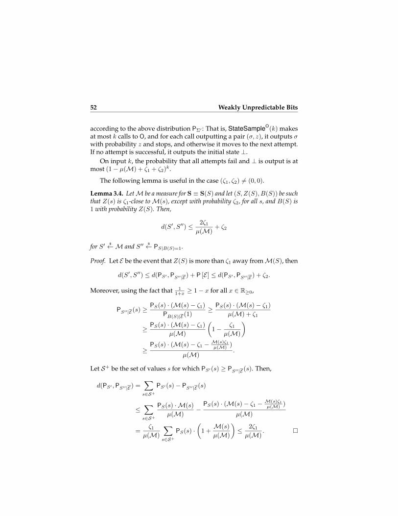
52 Weakly Unpredictable Bits
according to the above distribution PΣ′ : That is, StateSampleO(k) makesat most k calls to O, and for each call outputting a pair (σ, z), it outputs σwith probability z and stops, and otherwise it moves to the next attempt.If no attempt is successful, it outputs the initial state ⊥.
On input k, the probability that all attempts fail and ⊥ is output is atmost (1− µ(M) + ζ1 + ζ2)k.
The following lemma is useful in the case (ζ1, ζ2) 6= (0, 0).
Lemma 3.4. LetM be a measure for S ≡ S(S) and let (S,Z(S), B(S)) be suchthat Z(s) is ζ1-close toM(s), except with probability ζ2, for all s, and B(S) is1 with probability Z(S). Then,
d(S′, S′′) ≤ 2ζ1µ(M)
+ ζ2
for S′ $←M and S′′ $← PS|B(S)=1.
Proof. Let E be the event that Z(S) is more than ζ1 away fromM(S), then
d(S′, S′′) ≤ d(PS′ ,PS′′|E) + P [E ] ≤ d(PS′ ,PS′′|E) + ζ2.
Moreover, using the fact that 11+x ≥ 1− x for all x ∈ R≥0,
PS′′|E(s) ≥PS(s) · (M(s)− ζ1)
PB(S)|E(1)≥ PS(s) · (M(s)− ζ1)
µ(M) + ζ1
≥ PS(s) · (M(s)− ζ1)
µ(M)
(1− ζ1
µ(M)
)
≥PS(s) · (M(s)− ζ1 − M(s)ζ1
µ(M) )
µ(M).
Let S+ be the set of values s for which PS′(s) ≥ PS′′|E(s). Then,
d(PS′ ,PS′′|E) =∑s∈S+
PS′(s)− PS′′|E(s)
≤∑s∈S+
PS(s) · M(s)
µ(M)−
PS(s) · (M(s)− ζ1 − M(s)ζ1µ(M) )
µ(M)
=ζ1
µ(M)
∑s∈S+
PS(s) ·(
1 +M(s)
µ(M)
)≤ 2ζ1µ(M)
.

3.2 The Hardcore Lemma for System-Bit Pairs 53
Procedure EstimateWinO(A, µ(M), γ): // Adv. A, µ(M), γ ∈ [0, 1]
r :=
(1
γ− 2ζ1µ(M)
−ζ2
)2
k
for all i = 1, . . . , r doσ′i
$← StateSampleO(k/ log
(1
1−µ(M)+ζ1+ζ2
))oi := A(AS[σ′i])⊕AB [σ′i]
return 1r
∑ri=1 oi
Figure 3.3: The procedure EstimateWin given in Example 3.6.
Example 3.6. Let (S, B) ≡ (S(S), B(S)) be a cc-stateless system-bit pairwith efficient implementation A(S,B), and let A be an adversary: Wepresent a procedure (called EstimateWin and illustrated in Figure 3.3)which, for all measuresM for (S, B), estimates the probability
P[A(S(S′)) = B(S′)
∣∣S′ $←M]
within target error γ > 2ζ1µ(M) + ζ2, except with negligible probability,
given oracle access to a (ζ1, ζ2)-sampler O for M and A(S,B) with poly-nomial length. For efficiency, we require that γ − 2ζ1
µ(M) − ζ2 is noticeable,and that µ(M)−ζ1−ζ2 is noticeable. We use the notation (AS[σ′i], AB [σ′i])to denote the two components of the same instance of (S, B) simulatedby A(S,B). (Note that the procedure runs a new instance of A at everyiteration of the for all loop.)
First, by the discussion in Example 3.5, StateSample outputs a statewith the wrong distribution with probability at most
r · (1− µ(M) + ζ1 + ζ2)k/ log
(1
1−µ(M)+ζ1+ζ2
)= r · 2−k,
which is negligible for the given r. Assuming that the wrong distributionis never output, then (AS[σ′i], AB [σ′i]) ≡ (S(S′′), B(S′′)), with S′′ as inLemma 3.4. Consequently, by Hoeffding’s inequality (Lemma 2.1), o :=1r
∑ri=1 oi is an estimate of P [A(S(S′′)) = B(S′′)] with error γ− 2ζ1
1−µ(M)−ζ2, except with negligible probability. Moreover, by Lemma 3.4,
|P [A(S(S′)) = B(S′)]− P [A(S(S′′)) = B(S′′)]| ≤ d(S′, S′′)
≤ 2ζ1µ(M)
+ ζ2,

54 Weakly Unpredictable Bits
as one special distinguisher for S′ and S′′ outputs one if and only ifA(S(X)) = B(X) for X = S′ or X = S′′. Therefore, the estimate o is(by the triangle inequality) at most γ away from the actual value.
Note that running EstimateWin with parameter 1− ε ≤ µ(M) insteadof µ(M) would also produce an estimate which has at most error γ, as itcan be verified by inspection.
3.2.3. The Hardcore Lemma for System-Bit Pairs
In the following, for understood parameters γ, ε, ζ1, and ζ2, we define
ϕhc :=6400
γ2(1− ε)4· ln(
160
γ(1− ε)3
)and ψhc :=
200
γ2(1− ε)4ζ21
· ln(
2
ζ2
).
We now state the Hardcore Lemma for cc-stateless system-bit pairs.
Theorem 3.5 (HCL for System-Bit Pairs). Let (S, B) ≡ (S(S), B(S)) bea cc-stateless system-bit pair admitting an implementation A(S,B) with spacecomplexity sA(S,B)
. Furthermore, for some integers t, q > 0 and some ε ∈ [0, 1),
Guesst,q(B |S) ≤ ε.
Then, for all 0 < ζ1, ζ2 < 1 and all 0 < γ ≤ 12 , there exists a measureM for
(S, B) with µ(M) ≥ 1− ε such that the following two properties are satisfied:
(i) For S′ $←M, t′ := t/ϕhc, and q′ := q/ϕhc,
Guesst′,q′(B(S′) |S(S′)) ≤ γ.
(ii) There exists a (ζ1, ζ2)-sampler forM and A(S,B) with length sA(S,B)(q′ ·
ψhc). If (S(s), B(s)) is deterministic for all s, then there exists a (0, 0)-sampler forM and A(S,B) with length sA(S,B)
((7 · γ−2 · (1− ε)−3) · q′).
In the remainder of this section, we outline the proof intuition andgive some remarks on the above statement, while the full proof is post-poned to the next section (Section 3.2.4). A uniform version of Theo-rem 3.5 is given below in Section 3.2.8.
PROOF OUTLINE. The proof, which is by contradiction, extends in anumber of ways previous proofs by Impagliazzo [Imp95] and by Holen-stein [Hol05]. It starts by assuming that Theorem 3.5 is wrong, that is,

3.2 The Hardcore Lemma for System-Bit Pairs 55
that for any measureM on S with µ(M) ≥ 1− ε and such that a (ζ1, ζ2)-sampler for M and A(S,B) with the desired length exists, there also ex-ists an adversary A with time complexity t′ and making q′ queries suchthat GuessA(B(S′) |S(S′)) > γ for S′ $← M. Under this assumption,the proof builds an adversary A′ with time complexity t and making q
queries such that GuessA(B |S) > ε, hence contradicting the assumedhardness of guessing B given access to S.
The proof relies on the quantity NA(s) :=∑
A∈AGuessA(B(s) |S(s))measuring the overall performance of a collection A of deterministic ad-versaries in guessing B(s) when interacting with S(s) for given a states ∈ S. Additionally, we letMA,τ : S → [0, 1] be the measure associatedwith A and a threshold τ ∈ N such that elements for which A is worst,i.e., NA(s) ≤ τ , are given high weight (i.e. MA,τ (s) = 1), whereas ele-ments for whichA performs well, i.e., NA(s) ≥ τ + 1
γ(1−ε) , are not chosen(MA,τ (s) = 0). An intermediate measure value is assigned to states notfalling into one of these two categories. In particular,M∅,0 is the all-onemeasure (i.e., PM equals the initial state distribution PS), which has den-sity 1 ≥ 1 − ε. A crucial property, which we show, is that MA,τ alwaysadmits a (ζ1, ζ2)-state sampler for all A and τ .
The adversary A′ is then built as follows: Starting with A := ∅ andτ := 0, we iteratively find a deterministic adversary A such that
GuessA(B(S′) |S(S′)) > γ
for S′ $← MA,τ and add it to A. (Such A exists by the assumption thatTheorem 3.5 is wrong and the fact that a (ζ1, ζ2)-sampler exists for themeasureMA,τ .)
The process is repeated (possibly increasing τ to ensure that µ(MA,τ ) ≥1−ε), until either for all events E defined on S with P [E ] = 1−ε we haveE[GuessA(B(S′) |S(S′))
]> γ′ (for A
$← A, S′ $← PS|E , and γ′ slightly
smaller than γ) or we have P [NA(S) ≥ γ · |A|] ≥ 1 − 1−ε4 . For each of
both cases, we give an adversary A′ using the obtained collection A andguessing B from S with advantage better than ε. Furthermore, a majorpart of the proof consists of proving that this procedure terminates afterat most 7 · γ−2 · (1− ε)−3 iterations.
SOME ADDITIONAL REMARKS. We briefly discuss some additional pointsconcerning the statement of Theorem 3.5, which highlight the differenceswith the information-theoretic counterpart (Theorem 3.3).

56 Weakly Unpredictable Bits
Remark 3.3. A first natural question is whether the Hardcore Lemma canalso be proven for M defined on the randomness of the efficient imple-mentation A(S,B), hence fully dispensing with the concept of a state sam-pler and extend the result beyond cc-stateless systems. Yet all existingreductions in proofs of the Hardcore Lemma require repeated sequen-tial executions of adversaries providing independent outputs, and henceinherently require a cc-stateless representation of the system-bit pair.
Remark 3.4. Let (S, B) ≡ (S(S), B(S)) be a system-bit pair such thatGuessq(B |S) ≤ ε and, additionally, (S(s), B(s)) is deterministic for alls (or at least stateless). In both cases, even in the information-theoreticsetting, we cannot define an eventA on S with probability 1−ε such thata q-query adversary can only guess the bit B with probability 1
2 underthe condition that the eventA occurs. That is, a security loss is necessary.
We briefly illustrate this in the case q = 1. (Counterexamples forq > 1 can also be found.) For uniform independent two-valued ran-dom variables R00, R01 ∈ 0, 1, R10, R11 ∈ 1, 2, and B ∈ 0, 1, con-sider the cc-stateless system-bit pair (S(R00, R01, R10, R11, B), B). Oninput x ∈ 0, 1, the system S(r00, r01, r10, r11, b) returns rbx. Clearly,Guess1(B |S) = 1
2 : The optimal 1-query adversary A∗ queries 0, andoutputs 0 if it obtains a value in 0, 1, and 1 if it obtains 2.
Consider an event A such that the bit B can only be guessed withprobability 1
2 when A occurs: We need
PAR00R01R10R11B(r00, r01, r10, r11, b) = 0
whenever b = 0 and (r00, r01) 6= (1, 1), as well as whenever b = 1 and(r10, r11) 6= (1, 1), as otherwise there exists an adversary guessing B withnon-zero advantage conditioned on A occurring. But then,
P [A] ≤ 1
2· 1
4+
1
2· 1
4=
1
4< 1− 1
2.
Remark 3.5. It is not known whether the Hardcore Lemma can be ex-tended beyond cc-stateless system-bit pairs. However, we can show thatno such statement can hold with respect to arbitrary (but efficiently im-plementable) system-bit pairs. To see this, first remark that every sys-tem with MBO S can be turned into a system-bit pair (S′, B) such thatGuesst(B |S′) = νt(S), where νt(S) denotes the probability of the MBObecoming 1 maximized over all users with time complexity t. Let simplyS′ choose a secret uniform random bit B, and then behave as S. If theMBO turns one, then S′ hands the bit B over to the adversary. Clearly, if

3.2 The Hardcore Lemma for System-Bit Pairs 57
NA(s)
0 τ + 1γ(1−ε)τ
1
0
MA,τ(s)
N
WA,τ(s)
Figure 3.4: Measure MA,τ (s) as a function of NA(s). In particular, thegray area represents WA,τ (s) given that NA,τ (s) = N .
the MBO is 0, then B cannot be guessed with probability better than 12 ,
whereas if the MBO turns one, the adversary learns the bit and can guessit with probability 1.
In the setting where all parties (the adversary and the systems) sharesome initial random parameter (such as a public key), under reason-able assumptions there exist (cf. [BIN97, PW07]) systems12 S with MBOsuch that νt(S) ≤ ε for all polynomial t and some constant ε, whereasνt′(S1‖ . . . ‖Sm) ≈ ε holds already for very small t′. This yields a system-bit pair (S, B) where guessing B1, . . . , Bm for m independent instances(S1, B1), . . . , (Sm, Bm) is not harder than guessing B when interactingwith S. This implies, for example, that the XOR Lemma, which we provebelow and follows from Theorem 3.5, does not hold for such system-bitpairs.
3.2.4. High-Level Description of the Proof of Theorem 3.5
In this section, we present a full proof of the Hardcore Lemma for system-bit pairs (Theorem 3.5). At a high level, our proof follows Holenstein’sproof of the tight uniform13 Hardcore Lemma given in [Hol05] (which, inturn, was inspired by one of the proofs given by Impagliazzo [Imp95]).However, there are major differences (and difficulties) due to the fact thatwe are considering discrete interactive systems: In particular, for a given
12Although these original results address two-party protocols, one can see the honestparty as a system with MBO.
13Interestingly, no simpler approach appears to work despite the statement being provenbeing non-uniform.

58 Weakly Unpredictable Bits
s ∈ S the behavior of the system S(s) can be randomized (but stateless).Furthermore, we need to take into account the fact that we prove theexistence of a measure for which a sufficiently good state sampler exists.Also, unlike the case of random variables, it is crucial that no quantity inthe proof depends on the size of states S, as we cannot generally assumethem to be small. Another final difference (which turns out to be rathereasy to handle at the technical level) is that, contrary to the traditionalHardcore Lemma, we allow for the distribution PS of the state S to bedifferent than uniform.
INITIAL DEFINITIONS. For a collection A of (deterministic) adversaries,we define
NA(s) :=∑A∈A
GuessA(B(s) |S(s)),
for all s ∈ S. Note that |NA(s)| ≤ |A|. In particular, NA(s) provides aquantitative measure of the overall quality of the collectionA in guessingB(s) given access to S(s). For instance, NA(s)/ |A| gives the advantageof a randomly chosen A ∈ A in guessing B(s) while interacting withS(s). Moreover, for a non-negative integer τ ∈ N, we define the measureMA,τ : S → [0, 1] associated with A and τ such that
MA,τ (s) :=
1 if NA(s) ≤ τ ,1− (NA(s)− τ)γ(1− ε) if τ < NA(s) < τ + 1
γ(1−ε) ,0 if NA(s) ≥ τ + 1
γ(1−ε) .
The value MA,τ (s) is plotted as a function of NA(s) on Figure 3.4. Inother words, elements s ∈ S on which many adversaries in A are badare given more weight by the measure, whereas those for which manyadversaries are good are given no measure. Note that M∅,0 is the all-one measure, i.e., in particular the associated distribution PM equals PS .Hence, µ(M∅,0) ≥ 1− ε.
STRUCTURE OF THE PROOF. The proof is by contradiction. It starts byassuming that Theorem 3.5 is false. In other words, we assume that forsome γ, ζ1 and ζ2 the following holds:
Assumption ¬HC. For all measures M : S → [0, 1] withµ(M) ≥ 1 − ε such that a (ζ1, ζ2)-sampler forM and A(S,B)
with length14 ` := sA(S,B)(q′ ·ψhc) exists, there exists an adver-
sary A with time complexity t′ := t/ϕhc, making q′ := q/ϕhc
14In the case where (S(s), B(s)) is deterministic for all s ∈ S, we replace ψhc by 7 · γ−2 ·(1− ε)−3 and let ζ1 = ζ2 = 0.

3.2 The Hardcore Lemma for System-Bit Pairs 59
Procedure GoodEnough(A): // collection of adversaries A1: if A = ∅ then return false2: p := min
E:P[E]=1−εP[A(S(S)) = B(S)
∣∣A $← A, E]
3: ρ := P[NA(S) > γ · |A|]4: if p ≥ 1
2 + 14·(1−ε)·|A|γ ∨ ρ ≥ 1− 1−ε
4 then5: return true6: else7: return false
Procedure FindCollection: // no input1: A := ∅, τ := 02: while not GoodEnough(A) do3: if µ(MA,τ ) < 1− ε then4: τ := τ + 15: get deterministic A ∈ At′,q′ such that // see text
P[A(S(S′)) = B(S′)
∣∣S′ $←MA,τ]≥ 1 + γ
2
6: A := A ∪ A7: return A
Figure 3.5: Description of the procedure FindCollection used in the proofof Theorem 3.5.
queries, and such that
GuessA(B(S′) |S(S′)) > γ.
where S′ $←M.
The core of proof consists of the procedure FindCollection, specified inFigure 3.5, which, under Assumption ¬HC, outputs a collection of deter-ministic adversaries A such that |A| ≤ 7 · γ−2 · (1− ε)−3 and such that (atleast) one of the following two conditions is satisfied:
(A) P[NA(S) > γ · |A|] ≥ 1− 14 (1− ε)
(B) For all events E (defined by a probability distribution PE|S) such that

60 Weakly Unpredictable Bits
P[E ] = 1− ε, we have
P[A(S(S)) = B(S)
∣∣A $← A, E]≥ 1
2+
1
4 · (1− ε) · |A|γ .
We show how to derive, from a collectionA satisfying one of the two con-ditions, corresponding adversaries A(A) and A(B) with time complexityt and making q queries which guess B(S) given access to S(S) with ad-vantage greater than ε, contradicting the assumed hardness of (S, B).
Without loss of generality, throughout this proof we assume thatB(s)is determined by s.
THE PROCEDURE FindCollection. The procedure FindCollection (cf. Fig-ure 3.5) starts with A := ∅ and parameter τ = 0, and iteratively adds toA a deterministic15 adversary A with time complexity t′ and query com-plexity q′ such that
GuessA(B(S′) |S(S′)) > γ,
for S′ $← MA,τ . (Possibly, it first increments the value of τ by one toensure that µ(MA,τ ) ≥ 1 − ε.) Finally, it terminates when the collectionA satisfies (at least) one of conditions (A) or (B).
Note that the procedure FindCollection is to be seen as a process con-structing a collection, where in particular adversaries at Line 5 are notfound efficiently and explicitly, they are only guaranteed to exist by As-sumption ¬HC.
CORRECTNESS OF FINDCOLLECTION. In order for an adversary A as re-quired in Line 5 to exist under Assumption ¬HC, two conditions must bemet immediately before executing Line 5: First, the measureMA,τ musthave density at least 1− ε. Second, there must exist a (ζ1, ζ2)-sampler forMA,τ and A(S,B) with length ` ≤ sA(S,B)
(q′ · ψhc). The following lemmasshow that both conditions are always satisfied.
Lemma 3.6. At every execution of Line 5 in FindCollection, the conditionµ(MA,τ ) ≥ 1− ε holds.
Proof. The proof goes by induction. Clearly, it holds the first time Line5 is executed, since µ(M∅,0) = 1 ≥ 1 − ε, and hence τ is not increased.
15This can be assumed without loss of generality: Given a randomized adversary, anequally good deterministic adversary can be obtained by fixing its randomness to a goodvalue.
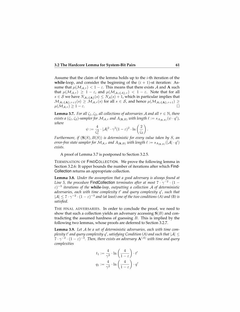
3.2 The Hardcore Lemma for System-Bit Pairs 61
Assume that the claim of the lemma holds up to the i-th iteration of thewhile-loop, and consider the beginning of the (i + 1)-st iteration: As-sume that µ(MA,τ ) < 1 − ε. This means that there exists A and A suchthat µ(MA,τ ) ≥ 1 − ε, and µ(MA∪A,τ ) < 1 − ε. Note that for alls ∈ S we have NA∪A(s) ≤ NA(s) + 1, which in particular implies thatMA∪A,τ+1(s) ≥ MA,τ (s) for all s ∈ S, and hence µ(MA∪A,τ+1) ≥µ(MA,τ ) ≥ 1− ε.Lemma 3.7. For all ζ1, ζ2, all collections of adversaries A and all τ ∈ N, thereexists a (ζ1, ζ2)-sampler forMA,τ and A(S,B) with length ` := sA(S,B)
(ψ · q′),where
ψ :=4
ζ21
· |A|2 · γ2(1− ε)2 · ln(
2
ζ2
).
Furthermore, if (S(S), B(S)) is deterministic for every value taken by S, anerror-free state sampler forMA,τ and A(S,B) with length ` := sA(S,B)
(|A| · q′)exists.
A proof of Lemma 3.7 is postponed to Section 3.2.5.
TERMINATION OF FINDCOLLECTION. We prove the following lemma inSection 3.2.6: It upper bounds the number of iterations after which Find-Collection returns an appropriate collection.
Lemma 3.8. Under the assumption that a good adversary is always found atLine 5, the procedure FindCollection terminates after at most 7 · γ−2 · (1 −ε)−3 iterations of the while-loop, outputting a collection A of deterministicadversaries, each with time complexity t′ and query complexity q′, such that|A| ≤ 7 · γ−2 · (1− ε)−3 and (at least) one of the two conditions (A) and (B) issatisfied.
THE FINAL ADVERSARIES. In order to conclude the proof, we need toshow that such a collection yields an adversary accessing S(B) and con-tradicting the assumed hardness of guessing B. This is implied by thefollowing two lemmas, whose proofs are deferred to Section 3.2.7.
Lemma 3.9. Let A be a set of deterministic adversaries, each with time com-plexity t′ and query complexity q′, satisfying Condition (A) and such that |A| ≤7 · γ−2 · (1 − ε)−3. Then, there exists an adversary A(A) with time and querycomplexities
t1 :=4
γ2· ln(
4
1− ε
)· t′
q1 :=4
γ2· ln(
4
1− ε
)· q′

62 Weakly Unpredictable Bits
such that GuessA(A)
(B |S) > ε.
Lemma 3.10. Let A be a set of deterministic adversaries, each with time com-plexity t′ and query complexity q′, satisfying Condition (B) such that |A| ≤7 · γ−2 · (1− ε)−3 . Then, there exists an adversary A(B) with time and querycomplexities
t2 :=6400
γ2(1− ε)4· ln(
160
γ(1− ε)3
)· t′
q2 :=6400
γ2(1− ε)4· ln(
160
γ(1− ε)3
)· q′
such that GuessA(B)
(B |S) > ε.
CONCLUDING THE PROOF. To conclude the proof, we observe that byAssumption ¬HC, Lemmas 3.6, 3.7, and 3.8, FindCollection outputs a col-lection A with |A| ≤ 7 · γ−2 · (1 − ε)−3 satisfying one of conditions (A)and (B). Then either Lemma 3.9 or Lemma 3.10 yields an adversary con-tradicting the assumed hardness of (S, B), as by definition of ϕhc, for thetime complexity we have t1 ≤ t and t2 ≤ t, as well as q1 ≤ q and q2 ≤ q.
3.2.5. Existence of State Samplers (Proof of Lemma 3.7)
The key observation is that given the collection A as well as black-boxaccess to the system-bit pair (S(S), B(S)), it is possible to compute a suf-ficiently good estimate of NA(S) (and thus ofMA,τ (S)) by letting (ran-domly chosen) adversaries from A sequentially interact with S(S) andcheck whether their outputs equal B or not. In particular, we can usethe algorithm A(S,B) in order to simulate (S(S), B(S)). Here, for nota-tional convenience, we assume that the algorithm A(S,B) first outputs thesimulated bit B, and subsequently implements S accordingly.
This is summarized by the random process OA,τ , which outputs avalid state of A(S,B), and is described in Figure 3.6, on top. We addi-tionally consider the idealized process O′A,τ (depicted in the lower part ofFigure 3.6) which, instead of using the algorithm A(S,B), uses the actualsystem-bit pair (S(S), B(S)) for a random S
$← PS , and produces an es-timate z(S) ofMA,τ (S) as in OA,τ , and finally outputs the pair (S, z(S)).Obviously, (A(S,B)[Σ], Z) for (Σ, Z)
$← OA,τ and (S(S), B(S), z(S)) for(S, z(S))
$← O′A,τ are exactly the same, that is, the equivalence
(A(S,B)[Σ], Z) ≡ ((S(S), B(S)), z(S))

3.2 The Hardcore Lemma for System-Bit Pairs 63
Sampler OA,τ : // collection of adversaries A, τ ∈ N
b$← A(S,B) // run A(S,B) to get the bit B
σ := state of A(S,B) after outputting B
ψ := 4ζ21· |A|2 · γ2(1− ε)2 · ln
(2ζ2
)for all i := 1, . . . , ψ do
A$← A
vi := A(A(S,B)[σ])⊕ b⊕ 1 // 1 if correct, 0 elseσ := last state of A(S,B) after interacting with A
N := 2|A| ·(
1ψ
∑ψi=1 vi − 1
2
)z := max0,min1, 1− (N − τ)γ(1− ε)return (σ, z)
Sampler O′A,τ : // collection of adversaries A, τ ∈ N
s$← PS
ψ := 4ζ21· |A|2 · γ2(1− ε)2 · ln
(2ζ2
)for all i := 1, . . . , ψ do
A$← A
vi(s) := A(S(s))⊕B(s)⊕ 1 // 1 if correct, 0 elseN(s) := 2|A| ·
(1ψ
∑ψi=1 vi(s)− 1
2
)z(s) := max0,min1, 1− (N(s)− τ)γ(1− ε)return (s, z(s))
Figure 3.6: Top: Construction of the state sampler OA,τ for MA,τ andA(S,B). Bottom: Idealized state sampler O′A,τ used in the proof ofLemma 3.7.

64 Weakly Unpredictable Bits
holds, due to the fact that A(S,B) implements (S, B). Therefore, in orderto finish the proof of property (ii) in Definition 3.3, it suffices to analyzethe quality of the estimate z(S) output by O′A,τ : Let us fix s ∈ S and
consider the random variable V (s) obtained by sampling a random A$←
A and then letting V (s) := 1 if A(S(s)) = B(s), and V (s) := 0 otherwise.Then, note that
E [V (s)] =1
|A|∑A∈A
P[A(S(s)) = B(s)]
=1
|A|∑A∈A
(1
2+
GuessA(B(s) |S(s))
2
)=
1
2+NA(s)
2|A| .
Since (S(S), B(S)) is cc-stateless, the pair (S(s), B(s)) is stateless (and inparticular, S(s) is stateless), and the values assigned to v1(s), . . . , vψ(s)are independent with the same distribution as V (s). In particular, wehave E [vi(s)] = E [V (s)] for all i ∈ 1, . . . , ψ. The event that z(s) isa bad estimate, i.e., that |z(s)−MA,τ (s)| > ζ1, implies in particular∣∣N(s)−NA(s)
∣∣ > ζ1γ(1−ε) and
∣∣∣ψ−1∑ψi=1 vi(s)− E [V (s)]
∣∣∣ > ζ12|A|γ(1−ε) .
We conclude by applying Hoeffding’s inequality (Lemma 2.1),
P [|z(s)−MA,τ (s)| > ζ1] ≤ P
[∣∣N(s)−NA(s)∣∣ > ζ1
γ(1− ε)
]≤ P
[∣∣∣∣∣ 1
ψ
ψ∑i=1
vi(s)− E [V (s)]
∣∣∣∣∣ > ζ12|A|γ(1− ε)
]
≤ 2e− ζ21
4|A|2γ2(1−ε)2ψ
= ζ2,
by the choice of ψ.
In the case where (S(S), B(S)) is deterministic given S, then a muchsimpler (and error-free) state sampler can be built: Namely, it is sufficientto let all adversaries A ∈ A interact (sequentially) with S (simulated byA(S,B)), rather then choosing them randomly, and set vi as above. Per-forming the analysis as above (via the ideal process O′A,τ ), we see thatN(s) indeed equals NA(s), and thus the estimate is always correct.

3.2 The Hardcore Lemma for System-Bit Pairs 65
3.2.6. The Procedure FindCollection Terminates (Proof of Lemma 3.8)
Similarly to the proofs in [Imp95, Hol05], we define for all collections ofadversaries A, all τ ∈ N and all s ∈ S the quantity
WA,τ (s) :=
τ −NA(s) + 1
2γ(1−ε) if NA(s) ≤ τ ,MA,τ (s)
2
[τ + 1
γ(1−ε) −NA(s)]
if τ < NA(s) < τ + 1γ(1−ε) ,
0 else.
This quantity is to be interpreted as the area underMA,τ (s), starting fromNA(s), as depicted in Figure 3.4. We also define the weighted average ofWA,τ (s) as
W (A, τ) := E [WA,τ (S)] =∑s∈S
PS(s) ·WA,τ (s).
In the following, we study the evolution of this quantity in order to provetermination for the execution of FindCollection. In particular, there aretwo causes for a change in the value of W at each iteration: First, anadversary A is always added to A. Second, the value τ is possibly incre-mented by one before the adversary is added. The following two claimsanalyze these two cases. We point out that the analysis is more involvedthan the one of [Hol05], due to the different termination condition andthe underlying distribution being arbitrary and not necessarily uniform.
The first claim shows that if we add an adversary to A in Line 5, thenW (A ∪ A, τ) is smaller than W (A, τ) by at least γ(1−ε)
2 .
Claim 1. Let A be a collection of adversaries and let τ ∈ N be such thatµ(MA,τ ) ≥ 1− ε. Moreover, let A /∈ A be an adversary such that
GuessA(B(S′) |S(S′)) > γ
for S′ $←MA,τ . Then W (A ∪ A, τ) ≤W (A, τ)− γ(1−ε)2 .
Proof. For all s ∈ S, the definition of NA yields NA∪A(s) = NA(s) +
GuessA(B(s) |S(s)), and consequently we obtain
WA∪A,τ (s) ≤WA,τ (s)−GuessA(B(s) |S(s)) · MA,τ (s) +γ(1− ε)
2.

66 Weakly Unpredictable Bits
Averaging over the choice of S yields
W (A ∪ A, τ) =∑s∈S
PS(s) ·WA∪A,τ (s)
≤W (A, τ) +γ(1− ε)
2−∑s∈S
PS(s) ·GuessA(B(s) |S(s)) · MA,τ (s).
However, note that if S′ $← MA,τ , then by definition PS′(s) := PS(s) ·MA,τ (s)/µ(MA,τ ), and hence∑
s∈SPS(s) ·GuessA(B(s) |S(s)) · MA,τ (s) =
= µ(MA,τ ) ·GuessA(B(S′) |S(S′)),
and the claim follows from µ(MA,τ ) ≥ 1−ε and GuessA(B(S′) |S(S′)) >γ.
The following claim additionally shows bounds on the variation ofW (A, τ) upon incrementing τ .
Claim 2. Let η > 0, let A be a collection of adversaries, and let τ ∈ N.Further assume that P [NA(S) > η] < 1− 1
4 (1− ε) and µ(MA,τ ) < 1− ε.Then,
W (A, τ + 1) ≤
W (A, τ) + (1− ε) + γ(1−ε)2 − γ(1−ε)2
8 if τ > η,W (A, τ) + (1− ε) + γ(1−ε)
2 if τ ≤ η.
Proof. For all s ∈ S we have
WA,τ+1(s) ≤WA,τ (s) +MA,τ (s) +γ(1− ε)
2.
In fact, ifNτ (s) ≤ τ , then we even haveWA,τ+1(s) ≤WA,τ (s)+MA,τ (s).From this we can infer
W (A, τ + 1) =∑s∈S
PS(s) ·WA,τ+1(s)
≤W (A, τ) +∑s∈S
PS(s) · MA,τ (s) +∑
s:NA(s)>τ
PS(s) · γ(1− ε)2
≤W (A, τ) + (1− ε) + P[NA(S) > τ ] · γ(1− ε)2
.

3.2 The Hardcore Lemma for System-Bit Pairs 67
If τ > η, then P[NA(S) > τ ] ≤ P[NA(S) > η] ≤ 1− 1−ε4 , and thus
W (A, τ + 1) ≤W (A, τ) + (1− ε) +
(1− 1− ε
4
)· γ(1− ε)
2
= W (A, τ) + (1− ε) +γ(1− ε)
2− γ(1− ε)2
8
whereas if τ ≤ η, we can only conclude that W (A, τ + 1) ≤ W (A, τ) +
(1− ε) + γ(1−ε)2 .
In the following, let A(i) and τ(i) be the values of A and τ at thebeginning of the i-th iteration, i.e., when GoodEnough is invoked. Inparticular, |A(i)| = i − 1. We now show that under the assumption16
that P[NA(i)(S) > γ · (i− 1)
]< 1 − 1
4 (1 − ε) holds, then FindCollectionterminates satisfying Condition (B). To this end, we define the potentialfunction π such that the potential at the beginning of the i-th iteration is
π(i) := W (A(i), τ(i))− τ(i) · (1− ε).
Note that initially π(1) = W (∅, 0) − 0 · (1 − ε) = W (∅, 0) = 12γ(1−ε) . The
above two claims imply the following for all i’s:
π(i+1) ≤
π(i)− γ(1−ε)
2 if τ(i) = τ(i+ 1)π(i) if τ(i+ 1) = τ(i) + 1 and τ(i) ≤ γ · (i− 1)
π(i)− γ(1−ε)2
8 if τ(i+ 1) = τ(i) + 1 and τ(i) > γ · (i− 1).
In particular, it is important to note that the value π(i) never increases.The following claim proves that it also decreases sufficiently fast, reach-ing a negative value after 7 · γ−2 · (1 − ε)−3 iterations. Below, we showthat in this case, the corresponding collection A satisfies Condition (B).
Claim 3. For λ := 7 · γ−2 · (1− ε)−3 we have π(λ+ 1) < 0.
Proof. Assume, towards a contradiction, that the claim is wrong, i.e., wehave an execution of FindCollection such that after λ := 7 · γ−2 · (1− ε)−3
completed iterations we have π(λ+1) ≥ 0 at the beginning of the (λ+1)-st iteration. Consider the partition I= ∪ I+ = 1, . . . , λ, where I= arethe iterations i where τ was not increased, whereas in I+ the value of τ
16If this assumption is not satisfied, then GoodEnough will detect this, and return true,which in particular implies termination of FindCollection, returning the collectionA(i) sat-isfying Condition (A).

68 Weakly Unpredictable Bits
is increased. We also let I∗ := (1 − γ)−1 |I=| + 2, . . . , λ. Hence, for alli ∈ I∗ we have
τ(i) ≥ i− 1− |I=| > i− 1− (1− γ)(i− 1) = γ(i− 1),
since (1 − γ)−1 |I=| < i − 1 for all i ∈ I∗. Therefore, for each iterationi ∈ I∗, we have π(i+ 1) ≤ π(i)− γ(1−ε)2
8 , and note that
|I∗| = λ− |I=|
1− λ − 1.
Moreover, we have |I=| ≤ γ−2(1−ε)−2 < γ−2(1−ε)−3, as otherwise thiswould contradict π(λ+ 1) ≥ 0 by the first claim. Using γ ≤ 1
2 , we obtain|I∗| > 5γ−2(1− ε)−3 − 1, which in particular implies
π(λ+ 1) ≤ 1
2γ(1− ε) − |I∗| γ(1− ε)2
8<γ(1− ε)2
8− 1
8γ(1− ε) < 0,
which is a contradiction.
Finally, we show that if π(i) < 0, then the collection A(i) satisfiesCondition (B), and thus termination is achieved.
Claim 4. If π(i) < 0, then A(i) satisfies
P[A(S(S)) = B(S)
∣∣A $← A(i), E]≥ 1
2+
1
4 · (1− ε) · |A(i)| · γ
for all events E (defined by PE|S) such that P [E ] = 1− ε.
Proof. Let τ := τ(i) and A := A(i). Also let E be an arbitrary event(defined by PE|S) such that p := P [E ] = 1 − ε. Then, by the definition ofNA,
P[A(S(S)) = B(S)
∣∣A $← A, S ∈ E]
=1
2+
1
2(1− ε)|A| ·∑s∈S
PSE(s)·NA(s).
Note that for all s ∈ S it is easy to verify that
WA,τ (s) ≥ τ +1
2γ(1− ε) −NA(s),

3.2 The Hardcore Lemma for System-Bit Pairs 69
Adversary A(A): // expecting to interact with system S(s)
ϕA := 4γ2 · ln
(4
1−ε
)for all i := 1, . . . , ϕA do
A$← A
vi$← A(S(s))
return majority vi : i ∈ 1, . . . , ϕA
Figure 3.7: Adversary A(A).
and therefore∑s∈S
PSE(s) ·NA(s) ≥∑s∈S
PSE(s) ·[τ +
1
2γ(1− ε) −WA,τ (s)
]≥ P [E ] ·
(τ +
1
2γ(1− ε)
)−∑s∈S
PS(s) ·WA,τ (s)
≥ (1− ε) · τ +1
2γ−W (A, τ) ≥ 1
2γ.
The lemma follows by substituting this into the above equation.
Therefore, after at most 7 ·γ−2 · (1−ε)−3 executions of the while-loop,the procedure FindCollection outputs a set of adversaries which satisfiesat least one of Condition (A) and Condition (B).
3.2.7. Constructing the Final Adversaries
PROOF OF LEMMA 3.9. Recall that we assume that
P [NA(S) > γ · |A|] ≥ 1− 14 (1− ε) > 1− 1
2 (1− ε) = 1+ε2 .
The adversary A(A) proceeds as described in Figure 3.7.Let us fix s such that NA(s) > γ · |A|. Then, we denote as I(s) ∈ 0, 1
the indicator random variable which is 1 if a randomly sampled A$← A
interacting with S(s) is successful, outputting B(s). (Recall that B(s) isfully determined by s.) Note that
E [I(s)] = P[A(S(s)) = B(s)
∣∣A $← A]
=1
|A|∑A∈A
P [A(S(s)) = B(s)]
=1
2+
1
2 · |A|∑A∈A
GuessA(B(s) |S(s)) =1
2+NA(s)
2 · |A| >1 + γ
2.

70 Weakly Unpredictable Bits
For i = 1, . . . , ϕA, denote as Ii(s) the random variable indicating whethervi equals B(s) when interacting with S(s): Since S(s) is stateless, thevariables I1(s), . . . , IϕA(s) are independent, with E [Ii(s)] = E [I(s)] forall i = 1, . . . , ϕA. We can use this (combined with Hoeffding’s inequality)to derive an upper bound on the failure probability of A(A) given accessto S(s),
P[A(A)(S(s)) 6= B(s)
]= P
[1
ϕA
ϕA∑i=1
Ii(s) <1
2
]
≤ P
[1
ϕA
ϕA∑i=1
Ii(s) < E [I(s)]− γ
2
]< e−
γ2
4 ϕA = 1−ε4 ,
and therefore
P[A(A)(S(S)) = B(S)] > P [NA(S) > γ · |A|] ·(1− 1−ε
4
)≥(1− 1−ε
4
)·(1− 1−ε
4
)≥ 1− 1−ε
2 = 1+ε2 .
Note that we can fix the choice of ϕA adversaries A1, . . . ,AϕA for therandom choices of A maximizing the success probability of the resultingadversary A(A). The time and query complexity bounds t1 and q1 arethen clear.
PROOF OF LEMMA 3.10. We define the functions α, α1 : S → [−1, 1] suchthat
α(s) := 2 · P[A(S(s)) = B(s)
∣∣A $← A]− 1,
α1(s) := 2 · P[A(S(s)) = 1
∣∣A $← A]− 1
for all s ∈ S. We order the elements of S as s1, s2, . . . such that α(si) ≤α(si+1) for i = 1, 2, . . .. Then, let i∗ be the (unique) index such that∑i∗−1j=1 PS(sj) < 1 − ε, but
∑i∗
j=1 PS(sj) ≥ 1 − ε. We define the eventE such that
PE|S(si) :=
1 if i < i∗,(1−ε)−
∑i∗−1j=1 PS(sj)
PS(si∗ ) if i = i∗,
0 if i > i∗,

3.2 The Hardcore Lemma for System-Bit Pairs 71
Adversary A(B): // expecting to interact with system S(s)
ϕB := 6400γ2(1−ε)4 · ln
(160
γ(1−ε)3
)for all i := 1, . . . , ϕB do
A$← A
vi$← A(S(s))
α1 := 2 ·(
1ϕB
∑ϕBi=1 vi − 1
)return 1 with probability max
0,min
1, 1
2 + α1
2(α∗− γ(1−ε)2
20
)
Figure 3.8: Adversary A(B).
and define α∗ := α(si∗). It is easy to verify that P [E ] = 1 − ε, and hence(recall that |A| ≤ 7 · γ−2 · (1− ε)−3)
P[A(S(S)) = B(S)
∣∣A $← A, E]≥ 1
2+
1
4(1− ε)|A|γ
>1
2+γ(1− ε)2
40.
This implies α∗ > γ(1−ε)2
20 , as otherwise this would contradict the abovelower bound on the guessing probability of a randomly chosen A fromthe collection A. We consider the adversary A(B) specified in Figure 3.8.
In the following, we assume that the above adversary is run on S(s)for some fixed s ∈ S . Denote as v1(s), . . . , vϕB (s) and α1(s) the vari-ables obtained during the interaction. Since S(s) is stateless, the valuesassigned to v1(s), . . . , vϕB (s) are independent, and distributed as the out-put V (s) of a randomly chosen A
$← A accessing S(s), which satisfies
E [V (s)] = P[A(S(s)) = 1
∣∣A $← A]
= 12 + α1(s)
2 .
Let G = G(s) be the event that |α1(s)− α1(s)| ≤ γ(1−ε)2
40 : By Hoeffding’s

72 Weakly Unpredictable Bits
inequality,
P[G]
= P
[|α1(s)− α1(s)| > γ(1− ε)2
40
]= P
[∣∣∣∣∣ 1
ϕB
ϕB∑i=1
vi(s)− E [V (s)]
∣∣∣∣∣ > γ(1− ε)2
80
]
≤ 2e−(γ(1−ε)2
80
)2
ϕB=γ(1− ε)3
80.
For all s ∈ S, define α(s) to be α1(s) if B(s) = 1, and −α1(s) if B(s) = 0,and note that by inspection
P[A(B)(S(s)) = B(s)
]= min
1,1
2+
α(s)
2(α∗ − γ(1−ε)2
20
) .
For any s such that PE|S(s) > 0, then α(s) ≥ α∗, and conditioned on the
event G, we have α(s) ≥ α∗ − γ(1−ε)2
40 , and thus
P[A(B)(S(s)) = B(s)
∣∣G] = 1.
Moreover, for every other s ∈ S, we have
P[A(B)(S(s)) = B(s)
∣∣G] ≥ 1
2+α(s)− γ(1−ε)2
40
2.
Therefore,
P[A(B)(S(S)) = B(S)
∣∣ E ,G] > 1
2+γ(1− ε)2
40− γ(1− ε)2
80
=1
2+γ(1− ε)2
80.
We finally conclude that
P[A(B)(S(S)) = B(S)
]≥ P [G] · P
[A(B)(S(S)) = B(S)
∣∣G]≥ P
[A(B)(S(S)) = B(S)
∣∣G]− P[G]
= P [E ] · P[A(B)(S(S)) = B(S)
∣∣G, E]+ P
[E]· P[A(B)(S(S)) = B(S)
∣∣G, E]− P[G]
> ε · 1 +1
2(1− ε) +
γ(1− ε)3
80− P
[G]
=1 + ε
2,

3.2 The Hardcore Lemma for System-Bit Pairs 73
as we wanted to show. The time complexity t2 and the query complexityq2 are clear by inspection.
3.2.8. The Uniform Hardcore Lemma
In this section, we discuss a uniform version of Theorem 3.5 along simi-lar lines as the one from [Hol05]. In informal terms, the uniform state-ment differs in that we prove that, for every polynomial-time adver-sary A and for every noticeable function γ, there exists a good measureM =M(A, γ) (with a corresponding sampler) such that guessing B(S′)
given S(S′) is hard for A, provided S′$← M, even when given oracle
access to a sampler forM. This will be sufficient for the applications ofthe lemma. (In the following, we re-define ψhc := 7200
ζ21 (1−ε)4γ2 · ln
(2ζ2
)in
the uniform setting.)
Theorem 3.11 (Uniform Hardcore Lemma). Let (S, B) ≡ (S(S), B(S)) bea cc-stateless system-bit pair with an efficient implementationA(S,B) with spacecomplexity sA(S,B)
. Furthermore, for some ε ∈ [0, 1) (with 1− ε noticeable)
Guesspoly(B |S) ≤ ε.
For all noticeable ζ1 > 0, all ζ2 = 2−poly(k) > 0, and all 0 < γ ≤ 12 (such that
2ζ11−ε + ζ2 ≤ γ
4 and 1 − ε − ζ1 − ζ2 is noticeable), and for all polynomial-timeq′-query (uniform) oracle adversaries A(·), there exists a measureM for (S, B)with µ(M) ≥ 1− ε such that the following two properties are satisfied:
(i) There exists a (ζ1, ζ2)-sampler O for M and A(S,B) with length ` :=sA(S,B)
(q′ · ψhc). In particular, if (S(s), B(s)) is deterministic for all s,then O is a (0, 0)-sampler for M and A(S,B) with length sA(S,B)
((256 ·γ−2 · (1− ε)−3) · q′).
(ii) For S′ $←M, 17
GuessAO
(B(S′) |S(S′)) ≤ γ.
The length of the states returned by the sampler only depends on thenumber of queries q′, but is independent of the time complexity of A (andthe length of oracle queries A expects). Otherwise, it would be possiblethat the statement only holds for adversaries which cannot retrieve theoutput of the sampler.
17That is, A is given access to an oracle which upon each invocation ignores its input andreturns a state sampled according to the state sampler.

74 Weakly Unpredictable Bits
Rather than giving a full proof, we opt for pointing out the modifi-cations to be made to the proof of Theorem 3.5 to obtain a uniform re-duction. The techniques are similar to the ones of [Hol05], yet care isrequired due to the interactive setting and the inability to exactly com-pute P [A(S(s)) = B(s)]. Once again, we proceed by contradiction, andthe corresponding initial assumption, which we tacitly make from nowon, is modified as follows:
Assumption ¬HC’. There exist noticeable ζ1, γ, and ζ2 =2−poly(k) (with the property that 2ζ1
1−ε+ζ2 ≤ γ4 and 1−ε−ζ1−ζ2
is noticeable), as well as a polynomially bounded q′, and anefficient q′-query oracle adversary A∗ which satisfies
GuessAO
(B(S′) |S(S′)) > γ
for all measuresM for (S, B) with µ(M) ≥ 1 − ε admitting a(ζ1, ζ2) state-sampler O for A(S,B) with length `, and S′ $←M.
In particular, we consider the general case where (S(s), B(s)) is possiblyrandomized. (The deterministic statement will follow in the same way asin the non-uniform case.)
The following lemma transforms A∗ into a more convenient form.
Lemma 3.12. There exists an efficient oracle adversary B∗ which, for all mea-sures M for (S, B) with µ(M) ≥ 1 − ε admitting a (ζ1, ζ2)-sampler O forA(S,B) with length `, outputs with overwhelming probability, given oracle ac-cess to O, an efficient deterministic q′-query adversary A (making no oraclequeries) such that
GuessA(B(S′) |S(S′)) > γ/6
for S′ $←M.
Proof. The adversary B∗ repeats the following, until successful: First, itchooses the random coins r for A∗ and makes sufficiently many oraclequeries in advance, returning values (σ1, z1), (σ2, z2), . . .. Then, it esti-mates, using EstimateWin with target error γ/6 (cf. Example 3.6), the ad-vantage of A∗ in guessingB(S′) given access to S(S′) with fixed random-ness r and oracle answers (σ1, z1), (σ2, z2), . . .. If the estimate is largerthan γ/3, it outputs A∗ with hard-coded random bits and query answers.
By the property of EstimateWin, if an adversary is output, its advan-tage is larger than γ/6 with overwhelming probability. Also note that

3.2 The Hardcore Lemma for System-Bit Pairs 75
in each attempt, random coins and oracle answers such that the result-ing adversaries achieves advantage at least γ/2 are sampled with prob-ability at least γ/2 by a Markov-like argument. In this case, an adver-sary is output by B∗, except with negligible probability. Moreover, afterΘ(
klog(1/(1−γ/2))
)attempts, such good random coins and oracle answers
are sampled except with probability O(2−k).
To ensure a consistent notation with the non-uniform case, in the re-mainder of this proof the parameter γ will equal γ/6 for the “actual” γthat appears in Assumption ¬HC’. The security reduction implementsa polynomial-time adversary A′ with GuessA
′(B(S) |S(S)) > ε by ini-
tially running the procedure FindCollection, using the oracle adversary(B∗)
O at Line 5 to obtain an adversary A to be added to the collection,and the state-sampler O for MA,τ accessed by B∗ is simulated (also inpolynomial-time) using the procedure given in the proof of Lemma 3.7.The final collectionA output when GoodEnough returns true is used ac-cording to A(A) or A(B) depending on whether (a variation of) Condition(A) or Condition (B) is satisfied.
However, the parameters ρ, p (both in GoodEnough), and α∗ (in A(B))cannot be computed exactly: The procedure GoodEnough is consequentlymodified, as in Figure 3.9, so that these parameters are estimated and theconditions in the if-statement are adapted accordingly. The next para-graphs describe the procedures Estimate-ρ and Estimate-p, as well as theresulting adaptations to A(A) and A(B). In particular, they will ensurethat GoodEnough returns true whenever one of Conditions (A) or (B) issatisfied, which implies that the analysis of termination for FindCollec-tion remains unchanged.
ESTIMATING ρ AND THE ADVERSARY A(A). The procedure Estimate-ρis described in Figure 3.10. We assume without loss of generality thatA(S,B) first outputs the bit B, and then simulates S. In particular, in eachiteration of the outer for-loop an independent instance (S(Si), B(Si)) issimulated using A(S,B), for independent S1, . . . , Sr. We will thereforeassume that equivalently the adversary Ai,j interact with S(Si) for all iand j, and the associated value N i is denoted as NA(Si). Note that theexpected value of the bj ’s (for a given Si = si) is
p(si) := P[A(S(si)) = B(si)
∣∣A $← A],

76 Weakly Unpredictable Bits
Procedure GoodEnough(A): // collection of adversaries A1: if A = ∅ then return false2: ρ := Estimate-ρ(A)3: p := Estimate-p(A)4: if ρ ≥ 1− 1−ε
3 ∨ p ≥ 12 + 5
32·(1−ε)·|A|γ then5: return true6: else7: return false
Figure 3.9: Procedure GoodEnough in the proof of the uniform HardcoreLemma.
Procedure Estimate-ρ(A): // collection of adversaries A
r :=(
121−ε
)2
· k
r′ :=(
64γ
)2
· kfor all i = 1, . . . , r dob
$← A(S,B)[⊥]σ0 := state of A(S,B) after outputting bfor all j = 1, . . . , r′ doAi,j
$← Abj := Ai,j(A(S,B)[σj−1])⊕ b⊕ 1σj := last state of A(S,B)[σj−1].
N i := 2 · |A| ·(
1r′
∑r′
j=1 bj − 12
).
ρ :=i :Ni>
3γ4 ·|A|
rreturn ρ
Figure 3.10: Procedure Estimate-ρ in the proof of the uniform HardcoreLemma.
and therefore, by the choice of r′, the average 1r′
∑r′
j=1 bj is at most γ/8away from p(si), except with probability 2e−k, by Hoeffding’s inequality,which means that NA(si) is at most 2 |A| γ/8 = |A| · (γ/4) away from

3.2 The Hardcore Lemma for System-Bit Pairs 77
NA(si). Moreover, we define
ρ↓ :=1
r|i : NA(Si) > γ · |A|| , ρ↑ :=
1
r|i : NA(Si) > (γ/2) · |A||
and observe that ρ↓ ≤ ρ ≤ ρ↑. Also, except with probability 2e−k, wehave
P[NA(S) ≥ γ
2· |A|
]≥ ρ↑ −
γ
4≥ ρ− 1− ε
12.
In other words, if ρ ≥ 1 − 1−ε3 , then we know that P
[NA(S) > γ
2 |A|]≥
1− 1−ε3 − 1−ε
12 = 1− 5(1−ε)12 . Additionally, we also know that, except with
probability 2e−k, we have
ρ ≥ ρ↓ ≥ P [NA(S) > γ · |A|]− 1− ε12
,
and thus, if Condition (A) holds, then ρ ≥ 1− 1−ε4 − 1−ε
12 = 1− 1−ε3 , and
thus GoodEnough returns true.Finally, we note that A(A) can simply be modified to work under the
condition that P[NA(S) > γ
2 |A|]≥ 1 − 5(1−ε)
12 by setting ϕA appropri-ately. Also, in the same way, we can ensure that its advantage is notice-ably higher than ε in order to compensate for the negligible error in thereduction.
ESTIMATING p AND THE ADVERSARY A(B) . The estimation of p is consid-erably more involved, and is described in Figure 3.11. As above, we asso-ciate with each iteration of the outer for-loop an instance (S(Si), B(Si)),and denote the corresponding pi as p(Si).
Note that a function p : S → R always defines an ordering18 of theelements of S as s1, s2, . . . such that p(si) ≤ p(si+1) for all i = 1, 2, . . ., andit is convenient to think of S as being sampled by first choosing a randomvariable R uniformly at random in [0, 1), and then letting S = S(R) := sifor the unique i such that R ∈
[∑i−1j=1 PS(sj),
∑ij=1 PS(sj)
). Then, we let
E∗ be the event thatR ∈ [0, 1−ε): Clearly, P [E∗] = 1−ε, and it is not hardto verify that E∗minimizes E [p(S) | E ] over all E with P [E ] = 1−ε definedon S.19 In the following, we consider the function p as in the previousparagraph: Note that E [p(S) | E ] := P
[A(S(s)) = B(s)
∣∣A $← A, E].
18In fact, there may be different possibilities, in which case we choose one arbitrarily.19If a better event E ′ assigns probability mass to [1 − ε, 1), and transferring the corre-
sponding probability mass to the range [0, 1− ε) would lead to an even better event.

78 Weakly Unpredictable Bits
Procedure Estimate-p(A): // collection of adversaries Ar := 1024 · γ2 · |A|2 · kr′ := 1024 · (1− ε)2 · γ2 · |A|2 · kfor all i = 1, . . . , r dob
$← A(S,B)[⊥]σ0 := state of A(S,B) after outputting bfor all j = 1, . . . , r′ doAi,j
$← Abj := Ai,j(AS[σj−1])⊕ b⊕ 1σj := last state of A(S,B)[σj−1]
pi := 1r′
∑r′
j=1 bj .reorder p1, . . . , pr such that pi ≤ pi+1 for all i = 1, . . . , r − 1i∗ := (1− ε)rp := 1
i∗−1
∑i∗−1i=1 pi
return p
Figure 3.11: Procedure Estimate-p in the proof of the uniform HardcoreLemma.
By the choice of r′, we have |p(Si)− p(Si)| ≤ 132(1−ε)|A|γ . for all
i = 1, . . . , r with overwhelming probability: In this case, by inspection,the average p output by Estimate-p using the values p(Si) is at most
132(1−ε)|A|γ away from the one obtained using p(Si) instead of pi(Si) forall i = 1, . . . , r.
Therefore, from now on, we analyze the case where the pi := p(Si)’sare used. In particular, let Ri ∈ [0, 1) be associated to Si and let E∗be defined as above for the function p. Using the Hoeffding’s boundtwice, we can show that |Ri∗ − (1− ε)| ≤ γ
32|A|·γ with overwhelmingprobability. First, let Xi ∈ 0, 1 (for i ∈ 1, . . . , r be an the indica-tor random variable which is 1 if and only if Ri < 1 − ε − γ
32|A|·γ (withµ := E [Xi] = 1− ε− γ
32|A|·γ ). Then,
P
[1
r
r∑i=1
Xi ≥ 1− ε]
= P
[1
r
r∑i=1
Xi ≥ µ+1
32 |A| · γ
]≤ e−k,
which yieldsRi∗ ≥ 1−ε− 132|A|·γ with probability 1−e−k, since otherwise,
more than a fraction 1−ε of theRi’s would be smaller than 1−ε− 132|A|·γ .

3.3 The XOR Lemma for System-Bit Pairs 79
Symmetrically, one can show that except with probability e−k we haveRi∗ ≤ 1− ε+ 1
32|A|·γ .We now observe that conditioned on Ri∗ ∈ [0, 1), the average p of
p(Ri) (for i = 1, . . . , i∗−1) is the same as the average of p(R′1), . . . , p(R′i∗−1)for R′1, . . . , R′i∗−1 uniformly distributed in [0, Ri∗ ]. Therefore, by the Ho-effding bound, we have that the average p1, . . . , pi∗−1 is at most 1
32·(1−ε)|A|·γaway from E [p(S) |S ∈ [0, Ri∗ ]], except with probability 2e−k. In the spe-cific case where |Ri∗ − (1− ε)| ≤ 1
32γ|A| , we have, using Lemma A.1,
|E [p(S) |S ∈ [0, r]]− E [p(S) | E∗]| ≤ 1
32(1− ε) |A| γ ,
since maxRi∗ , (1− ε) ≥ 1− ε. Therefore, in the end we have
|p− p| ≤ 3 · 1
32γ(1− ε) · |A| · γ .
Thus, if the test p ≥ 12 + 5
32·(1−ε)·|A|·γ passes, then we are guaranteedthat p ≥ 1
2 + 116·(1−ε)·|A|·γ holds. Furthermore, if p ≥ 1
2 + 14(1−ε)·|A|·γ , as
guaranteed by Condition (B), then the test is also successful.Finally, we need to adapt A(B) to only use the guarantee that p ≥
12 + 1
16·(1−ε)·|A|·γ (which is unproblematic), and furthermore, we need toadditionally estimate α∗: This can be done as the computation of pi∗ inEstimate-p, we the difference that we compute
αi := 2 ·
1
r′
r′∑j=1
bj − 1
,
and take αi∗ as an approximation of α∗. Also, again we have to ensurethat the advantage is noticeably higher than ε to compensate for the neg-ligible error probability. We omit the details.
3.3. The XOR Lemma for System-Bit Pairs
This section presents the second main result of this chapter, the XORLemma for cc-stateless system-bit pairs. In analogy to the first part ofthis chapter, we start by considering the information-theoretic case as amotivation for the computational results. Then, Section 3.3.2 presents aproof of the XOR Lemma from the Hardcore Lemma which follows theinformation-theoretic intuition. Finally, Section 3.3.3 is devoted to a di-rect proof of the XOR Lemma achieving a somewhat stronger statement.

80 Weakly Unpredictable Bits
3.3.1. Setting and Information-Theoretic Intuition
We consider the setting with m system-bit pairs (S1, B1), . . . , (Sm, Bm).We are interested in upper bounding (as a function of the Guessqi(Bi |Si)for i = 1, . . . ,m) the advantage Guessq1,...,qm(B1⊕ · · ·⊕Bm |S1‖ · · · ‖Sm)of guessing the bitB1⊕· · ·⊕Bm given parallel access to S1, . . . ,Sm, whereat most qi queries to each system Si are allowed. That is, we considerthe most general attack where the adversary can query each subsystemSi individually at most qi times, adaptively depending on the answers ofqueries to other subsystems.
The following theorem shows that the advantage is upper boundedby the product of the individual advantages Guessqi(Bi |Si).
Theorem 3.13. For all q1, . . . , qm > 0,
Guessq1,...,qm(B1 ⊕ · · · ⊕Bm |S1‖ · · · ‖Sm) ≤m∏i=1
Guessqi(Bi |Si).
Proof. For all i = 1, . . . ,m, define for (Si, Bi) the corresponding system-bit pair with MBO (Si, Bi) which is guaranteed to exist by Theorem 3.3.Clearly,
Guessq1,...,qm(B1 ⊕ · · · ⊕Bm |S1‖ · · · ‖Sm) =
= Guessq1,...,qm(B1 ⊕ · · · ⊕ Bm | S1‖ · · · ‖Sm).
However, as long as there exists an i such that the MBO of (Si, Bi) is0, Property (ii) of Theorem 3.3 implies that the bit Bi is uniformly dis-tributed, and therefore the exclusive-or B1⊕· · ·⊕ Bm cannot be guessed,except with probability 1
2 . Therefore, for all adversaries A, with ν :=
νq1,...,qm(S1‖ · · · ‖Sm),
P[A(S1‖ . . . ‖Sm) = B1 ⊕ · · · ⊕ Bm
]≤ (1 − ν) · 1
2+ ν · 1 ≤ 1 + ν
2,
and by Theorem 2.4,
νq1,...,qm(S1‖ · · · ‖Sm) ≤m∏i=1
νqi(Si) =
m∏i=1
Guessqi(Bi |Si).

3.3 The XOR Lemma for System-Bit Pairs 81
3.3.2. XOR Lemma from the Hardcore Lemma
In this section we prove a generalization of Yao’s XOR Lemma [Yao82,GNW95] to system-bit pairs, which is a computational analogue of The-orem 3.13: We are given m instances20 (S1, B1), . . . , (Sm, Bm) of a cc-stateless system-bit pair (S, B) ≡ (S(S), B(S)) with the property thatGuesst′,q′(B |S) ≤ ε and admitting an implementation A(S,B) with timeand space complexities tA(S,B)
and sA(S,B), respectively. We prove that,
given access to all of S1, . . . ,Sm in parallel, the XOR B1 ⊕ · · · ⊕ Bm canonly be guessed with advantage at most εm + γ by an adversary with re-lated time complexity t and making at most q queries to each subsystemSi, where γ can be made arbitrarily small at the cost of reducing t and qwith respect to t′ and q′.21
Theorem 3.14 (XOR Lemma). For all integers t, q,> 0, all ε ∈ [0, 1), ζ1, ζ2 ∈(0, 1), and γ ∈
(0, 1
2
], if
Guesst′,q′(B |S) ≤ ε,
then,
Guesst,q,...,q(B1 ⊕ · · · ⊕Bm |S1‖ . . . ‖Sm) ≤ εm + 2m · (ζ1 + ζ2) + γ,
where t′ = ϕhc ·[t+O
((m− 1) ·
(l + tA(S,B)
(q, l)))]
and q′ = ϕhc · q, withl := sA(S,B)
(ψhc · q).
Proof. Let A be an adversary with time complexity t issuing q queries toeach subsystem S1, . . . ,Sm and outputting a guess B′ for B1 ⊕ · · · ⊕Bm.Further, using the Hardcore Lemma (Theorem 3.5), letM with µ(M) ≥1− ε be such that
Guesst′/ϕhc,q(B(S′) |S(S′)) ≤ γ (3.1)
for S′ $← M, and let O be the corresponding (ζ1, ζ2)-sampler forM andA(S,B) with length l = sA(S,B)
(ψhc · q).
20An analogous statement can easily be obtained if the instances are from differentsystem-bit pairs. However, we will prove such a general statement in Theorem 3.15 be-low, and for this version, opt for simplicity in order to illustrate an example application ofthe Hardcore Lemma.
21As pointed out in [GNW95], referring to a note by Steven Rudich, such a trade-off isunavoidable. A quantitative study of this trade-off follows from the work of Shaltiel andViola [SV08].

82 Weakly Unpredictable Bits
We consider an adversary A′ which, given access to S(S′), first sam-plesm pairs (Σ1, Z1), . . . , (Σm, Zm) using O, and subsequently flips inde-pendent bits U1, . . . , Um ∈ 0, 1, where PUj (1) := Zj for j = 1, . . . ,m.Then, it picks an i ∈ 1, . . . ,m (provided it exists) such that Ui = 1, andsimulates the interaction of A with
AS[Σ1] ‖ . . . ‖AS[Σi−1] ‖S(S′) ‖AS[Σi+1] ‖ · · · ‖AS[Σm],
where AS[Σj ] is the instance of S simulated by A(S,B)[Σj ] (with B′j beingthe associated bit), for j = 1, . . . ,m, j 6= i. When A outputs a bit B′,A′ outputs B′ ⊕⊕j 6=iB
′j . If no such i exists, A′ terminates directly by
returning a random bit. Clearly, A′ can equivalently be seen as samplingm independent pairs (S1, Z(S1)), . . . , (Sm, Z(Sm)), letting Uj be one withprobability Z(Sj), and replacing AS[Σj ] and B′j with S(Sj) and B(Sj) forall j = 1, . . . ,m, j 6= i. This does not alter the guessing advantage.
We also consider the adversary A′ where Z(Sj) is replaced byM(Sj)
for all j = 1, . . . ,m, and denote as U1, . . . , Um the corresponding inde-pendent bits. (Remark that PUj (1) = µ(M) ≥ 1− ε.) Analogously, in the
experiment where A interacts with S1‖ . . . ‖Sm, define the bits Uj accord-ingly. In both experiments, let E be the event that U1 = · · · Um = 0. Notethat P [E ] ≤ εm. Furthermore,
P[A′(S(S′)) = B(S′)
∣∣ E] = P[A(S1‖ . . . ‖Sm) = B1 ⊕ · · · ⊕Bm
∣∣ E] ,from which, using the facts that P
[A(S1‖ . . . ‖Sm) = B1 ⊕ · · · ⊕Bm
∣∣ E] ≤1 and that P
[A′(S(S′)) = B(S′)
∣∣ E] = 12 , we can upper bound p :=
P [A(S1‖ . . . ‖Sm) = B1 ⊕ · · · ⊕Bm] as
p ≤ P [E ] + (1− P [E ]) · P[A′(S(S′)) = B(S′)
∣∣ E]≤ P [E ]
2+ P [E ] · 1
2+ (1− P [E ]) · P
[A′(S(S′)) = B(S′)
∣∣ E]≤ εm
2+ P
[A′(S(S′)) = B(S′)
],
or, in other words
GuessA(B1⊕· · ·⊕Bm |S1‖ . . . ‖Sm) ≤ εm+GuessA′(B(S′) |S(S′)). (3.2)
Furthermore, note that for all j = 1, . . . ,m and b ∈ 0, 1
d(Uj , Uj) =∣∣∣PUj (b)− PUj (b)
∣∣∣ ≤ ζ1 + P [E ′] ≤ ζ1 + ζ2,
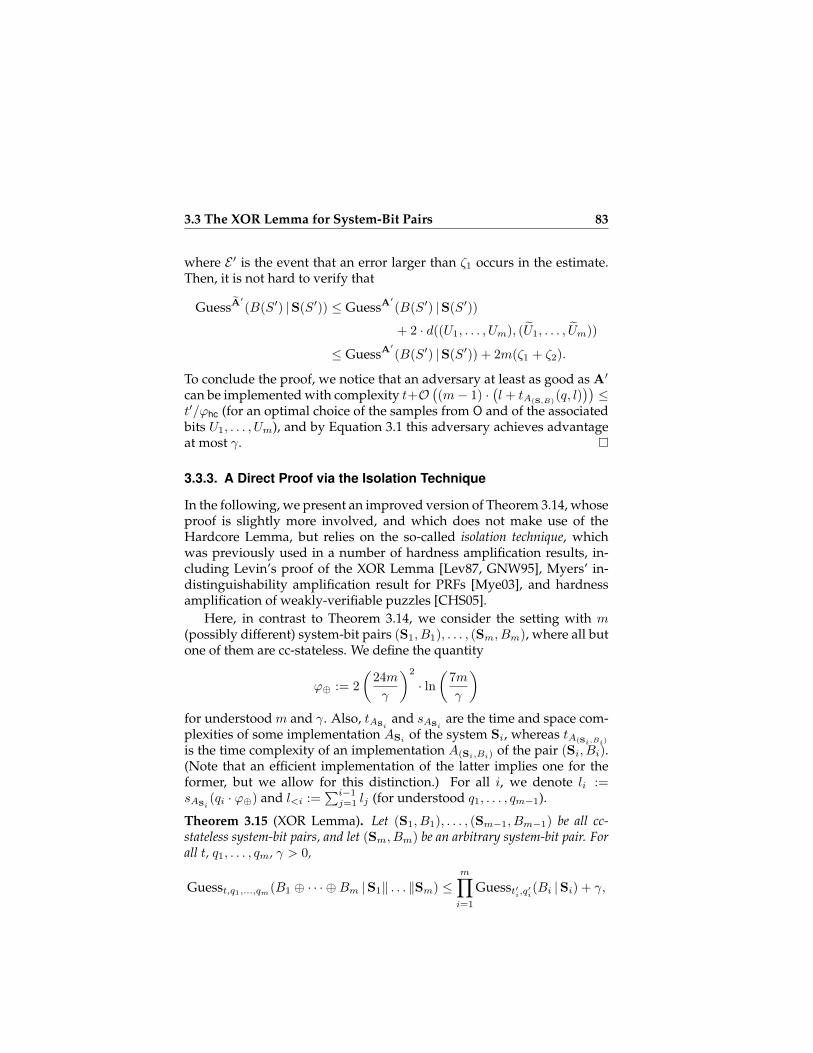
3.3 The XOR Lemma for System-Bit Pairs 83
where E ′ is the event that an error larger than ζ1 occurs in the estimate.Then, it is not hard to verify that
GuessA′(B(S′) |S(S′)) ≤ GuessA
′(B(S′) |S(S′))
+ 2 · d((U1, . . . , Um), (U1, . . . , Um))
≤ GuessA′(B(S′) |S(S′)) + 2m(ζ1 + ζ2).
To conclude the proof, we notice that an adversary at least as good as A′
can be implemented with complexity t+O((m− 1) ·
(l + tA(S,B)
(q, l)))≤
t′/ϕhc (for an optimal choice of the samples from O and of the associatedbits U1, . . . , Um), and by Equation 3.1 this adversary achieves advantageat most γ.
3.3.3. A Direct Proof via the Isolation Technique
In the following, we present an improved version of Theorem 3.14, whoseproof is slightly more involved, and which does not make use of theHardcore Lemma, but relies on the so-called isolation technique, whichwas previously used in a number of hardness amplification results, in-cluding Levin’s proof of the XOR Lemma [Lev87, GNW95], Myers’ in-distinguishability amplification result for PRFs [Mye03], and hardnessamplification of weakly-verifiable puzzles [CHS05].
Here, in contrast to Theorem 3.14, we consider the setting with m(possibly different) system-bit pairs (S1, B1), . . . , (Sm, Bm), where all butone of them are cc-stateless. We define the quantity
ϕ⊕ := 2
(24m
γ
)2
· ln(
7m
γ
)for understood m and γ. Also, tASi
and sASiare the time and space com-
plexities of some implementation ASi of the system Si, whereas tA(Si,Bi)
is the time complexity of an implementation A(Si,Bi) of the pair (Si, Bi).(Note that an efficient implementation of the latter implies one for theformer, but we allow for this distinction.) For all i, we denote li :=sASi
(qi · ϕ⊕) and l<i :=∑i−1j=1 lj (for understood q1, . . . , qm−1).
Theorem 3.15 (XOR Lemma). Let (S1, B1), . . . , (Sm−1, Bm−1) be all cc-stateless system-bit pairs, and let (Sm, Bm) be an arbitrary system-bit pair. Forall t, q1, . . . , qm, γ > 0,
Guesst,q1,...,qm(B1 ⊕ · · · ⊕Bm |S1‖ . . . ‖Sm) ≤m∏i=1
Guesst′i,q′i(Bi |Si) + γ,

84 Weakly Unpredictable Bits
where
t′i = l<i + ϕ⊕ ·
t+O
i−1∑j=1
tASj(qj , lj) +
m∑j=i+1
tA(Sj ,Bj)(qj)
and q′i = ϕ⊕ · qi for i = 1, . . . ,m− 1, whereas
tm = l<m + t+O
m−1∑j=1
tASj(qj , lj)
, q′m = qm.
The asymmetry of our proof technique allows (Sm, Bm) to be fullystateful.22 Furthermore, both t′m and q′m are much smaller then the corre-sponding terms t′i and q′i for i = 1, . . . ,m − 1. The full proof is given inthe next section.
3.3.4. Proof of Theorem 3.15
The proof of Theorem 3.15 relies on the so-called Isolation Lemma, whichreduces the situation where an adversary obtains an advantage δ · ε inguessing the XOR of the bits Bi ⊕ · · · ⊕ Bm for m − i system-bit pairs toeither an adversary guessing Bi from Si with advantage at least ε, or tothe situation where an adversary guesses Bi+1⊕· · ·⊕Bm for the system-bit pairs (Si+1, Bi+1), . . . , (Sm, Bm) with advantage at least δ. In contrastto similar lemmas in the literature, we give a more concrete statementwhich will be useful later on.
For the remainder of this section, we define, for an understood pa-rameter γ > 0,
ϕisol = 2
(24
γ
)2
· ln(
7
γ
).
Note that the value ϕ⊕ used above corresponds to the special case whereγ := γ/m for the understood parameter γ. The values l1, l2, . . . are de-fined as above (before the statement of Theorem 3.15) with respect toϕisol. Finally, we introduce the shorthands (for i ≤ j)
B[i,j] := Bi ⊕ · · · ⊕Bj ,S[i,j] := Si‖ . . . ‖Sj ,
AS[i,j][σi, . . . , σj ] := ASi [σi]‖ . . . ‖ASj [σj ].
22An incomparable generalization of the XOR Lemma for stateful interactive systems wasproposed by Halevi and Rabin [HR08]. However, it relies on sequential (rather than parallel)access to the systems S1, . . . ,Sm, which is not sufficient for the applications of this thesis.

3.3 The XOR Lemma for System-Bit Pairs 85
Lemma 3.16 (Isolation Lemma). Let i ∈ 1, . . . ,m − 1, let γ > 0, and letA be an adversary with complexity t making qj queries to Sj for j = 1, . . . ,m.Moreover, let σ1, . . . , σi−1 be valid states for AS1
, . . . , ASi−1, respectively, with
|σj | ≤ lj (for j = 1, . . . , i− 1), and let b[1,i−1] ∈ 0, 1. Assume that
GuessA(b[1,i−1] ⊕B[i,m] |AS[1,i−1][σ1, . . . , σi−1]‖S[i.m]) > δ · ε+ γ.
Then, at least one of the following two statements is true:
(i) There exists a valid state σi for ASi with |σi| ≤ li and a bit b[1,i] ∈ 0, 1such that
GuessA(b[1,i] ⊕B[i+1,m] |AS[1,i][σ1, . . . , σi]‖S[i+1.m]) > δ;
(ii) There exists an adversary A′i with running time t′i making q′i queries suchthat GuessA
′i(Bi |Si) > ε, and
t′i = l<i + ϕisol ·
t+O
i−1∑j=1
tASj(qj , lj) +
m∑j=i+1
tA(Sj ,Bj)(qj)
and q′i = ϕisol · qi.
The proof of the Isolation Lemma is postponed to Section 3.3.5. Thenext paragraph shows how the full XOR Lemma can be obtained from theIsolation Lemma. Note that we do not put priority on optimizing values(such as the function ϕisol defined above), but rather on having simplerexpressions, which are in particular independent of the upper bounds onthe underlying advantages.
FROM THE ISOLATION LEMMA TO THE XOR LEMMA. In the following,fix some t, q1, . . . , qm, γ > 0 and set γ := γ/(m− 1). Define t′i, q
′i as in the
statement of Theorem 3.15, and let εi := Guesst′i,q′i(Bi |Si).From now on, let A be the adversary with running time t making
q1, . . . , qm queries to the respective systems, and such that
GuessA(B[1,m] |S[1,m]) ≥ ε1 · · · εm + γ.
Define γi := (m − 1 − i) · γ for i = 0, . . . ,m − 1 and consider the state-ments STATi(σ1, . . . , σi, b) for a bit b ∈ 0, 1 and valid states σ1, . . . , σi

86 Weakly Unpredictable Bits
of AS1 , . . . , ASi respectively, with |σj | ≤ lj for j = 1, . . . , i which holds ifand only if
GuessA(b⊕B[i+1,m] |AS[1,i][σ1, . . . , σi]‖S[i+1,m]) ≥ εi+1 · · · εm + γi
≥ εi+1 · (εi+2 · · · εm + γi+1) + γ,
where we have used the facts that γi := γi−1 + γ and εi+1 ≤ 1. In par-ticular, by our assumption STAT0(0) holds. Furthermore, given that theassumption STATi(σ1, . . . , σi−1, b) holds for some i we apply the Isola-tion Lemma (Lemma 3.16). Note that condition (ii) cannot hold, as oth-erwise there exists an adversary A′i such that GuessA
′i(Bi |Si) > εi, but
this contradicts the assumed hardness of (Si, Bi), as we have defined εiwith respect to the maximal running time of a constructed adversary A′i.Therefore, condition (i) must hold: In other words, we have shown thatfor all i = 0, . . . ,m− 2
STATi(σ1, . . . , σi, b) =⇒ ∃σi+1, b′ : STATi(σ1, . . . , σi, σi+1, b⊕ b′),
where all the states σ1, σ2, . . . are valid for their respective implementa-tions and are such that |σi| ≤ li. Iterating the argument we obtain thatthere exist σ1, . . . , σm−1 and a bit b such that
GuessA(b⊕Bm |AS[1,m−1][σ1, . . . , σm−1]‖Sm) > εm + γm−1 = εm.
However, we can now consider the adversary
A′ := A(AS[1,m−1][σ1, . . . , σm−1]‖·)⊕ b
which, given access to Sm, simulates the adversary A interacting withthe system AS[1,m−1]
[σ1, . . . , σm−1]‖Sm, obtaining output b′, and finallyoutputs b ⊕ b′. Such an adversary has advantage larger than > εm, con-tradicting the assumed hardness of (Sm, Bm).
3.3.5. Proof of the Isolation Lemma
Throughout the proof, let (Si(·), Bi(·)) and S ∈ S be such that we have(Si(S), Bi(S)) ≡ (Si, Bi). Note that such a representation of (Si, Bi) ex-ists since the system-bit pair is assumed to be cc-stateless (as i ≤ m − 1).In particular, Bi(s) depends (without loss of generality) deterministicallyon the input s. For the remainder of this proof, it is convenient to defineγ′ := γ
4 , and for the system-bit pairs (Si+1, Bi+1), . . . , (Sm, Bm) (and the

3.3 The XOR Lemma for System-Bit Pairs 87
given states σ1, . . . , σi−1 in the statement of the Isolation Lemma) we usethe notation
M(·) := AS[1,i−1][σ1, . . . , σi−1]‖ · ‖S[i+1,m].
Note that these are only notational shorthands. In particular, the systemSj is correlated with the corresponding bit Bj for j ≥ i + 1 as in thesystem-bit pair (Sj , Bj). Moreover, we define α1, α : S → [−1, 1] suchthat for all s ∈ S
α1(s) := 2 · P[A(M(Si(s)))⊕ b[1,i−1] ⊕B[i+1,m] = 1]− 1,
α(s) := 2 · P[A(M(Si(s)))⊕ b[1,i−1] ⊕B[i+1,m] = Bi(s)]− 1.
By rearranging terms in the definition ofα (i.e. by moving b[1,i−1]⊕B[i+1,m]
to the right-hand side) we see that E[α(S)] > δ · ε+ γ by the assumptionof the lemma, and also α(s) = α1(s) if Bi(s) = 1, and α(s) = −α1(s) ifBi(s) = 0.
The remainder of the proof of the Isolation Lemma is subdivided intothe following two technical lemmas.
Lemma 3.17. If P[|α1(S)| > δ + γ′] > γ′, then there exists σi for ASi with|σi| ≤ li and bi ∈ 0, 1 such that
GuessA(b[1,i−1] ⊕ bi ⊕B[i+1,m] |M(ASi [σi]) > δ.
Lemma 3.18. If P[|α1(S)| > δ + γ′] ≤ γ′, then there exists an adversary A′iwith running time t′i and making q′i queries such that GuessA
′i(Bi |Si) > ε.
The Isolation Lemma is implied by these two lemmas, since eitherP[|α1(S)| > δ + γ′] > γ′ holds (and in this case Lemma 3.17 impliesstatement (i)), or P[|α1(S)| > δ + γ′] ≤ γ′ holds, which yields (ii).
The remainder of this section is devoted to proving the above twolemmas.
PROOF OF LEMMA 3.17. We define a random process SAMPLE (whichis depicted on the left-hand side of Figure 3.12) outputting a pair (σ, b),where σ is a valid state for ASi and b ∈ 0, 1 is a bit. The processSAMPLE lets ϕisol independent instances of A(·) := A(M(·)) ⊕ b[1,i−1] ⊕B[i+1,m]
23 sequentially interact with the same instance of Si, producing
23i.e. the adversary which for new independent instances of (Si+1, Bi+1), . . . , (Sm, Bm)simulates an interaction of A with AS[1,i−1]
[σ1, . . . , σi−1]‖S‖S[i+1,m], where S is thegiven system, and adds b[1,i−1] ⊕B[i+1,m] to its output to obtain the actual output

88 Weakly Unpredictable Bits
outputs o1, . . . , oϕisol (and denote by o their average). The instance of Si issimulated using ASi by letting, for j = 1, . . . , ϕisol, the j-th independentinstance of A interact withASi [σj−1], and setting σj to be the final state ofASi after such interaction (and σ0 := ⊥ is the empty, initial state for ASi ).Also, it sets σ := σϕisol . The process SAMPLE computes α1 := 2·o−1. If α1
is higher than δ, we expect GuessA(b[1,i−1]⊕1⊕B[i+1,m] |M(ASi [σ])) > δ(and the process hence outputs (σ, 1)), whereas if it is lower than −δ, weexpect GuessA(b[1,i−1]⊕ 0⊕B[i+1,m] |M(ASi [σ])) > δ (and SAMPLE out-puts (σ, 0)).
We consider a random experiment where SAMPLE samples a pair(σ, b), and we subsequently compute A(M(ASi [σ])) ⊕ b[1,i−1] ⊕ B[i+1,m].We define the event T that one of the if-statements within process SAMPLEis executed, and we show that under the assumption that P[|α1(S)| >δ + γ′] > γ′ we have P[T ] > 0 and
π1 ≥1 + δ
2, (3.3)
for
π1 := P[(σ, b)← SAMPLE : A(M(ASi [σ]))⊕ b[1,i−1] ⊕B[i+1,m] = b | T ].
Note that this is sufficient to obtain the statement of Lemma 3.17, as wecan choose a pair (σ, b) output by SAMPLE conditioned on the event T(note that this yields a well-defined distribution of pairs (σ, b)) maximiz-ing the above probability, and set σi := σ, b[1,i] := b[1,i−1] ⊕ b. Since Aissues at most qi queries, and the above process is repeated ϕisol times, wehave |σi| ≤ sASi
(qi · ϕisol) = li.In order to prove inequality (3.3), we consider a second sampling pro-
cess (called SAMPLE′ and depicted on the right-hand side of Figure 3.12)which samples s according to PS and subsequently computes the val-ues o1, . . . , oϕisol by letting ϕisol independent instances of A interact withSi(s). The process finally outputs the pair (s, b) with b being computedas in SAMPLE. In particular, we also denote here as T the event that oneof the two conditions in the if-statement is satisfied, and we define
π2 := P[(s, b)← SAMPLE′ : A(M(Si(s)))⊕ b[1,i−1] ⊕B[i+1,m] = b | T ].
A crucial observation is that the sampling processes SAMPLE andSAMPLE′ compute the values o1, . . . , oϕisol by letting multiple, indepen-dent, instances of A interact with the same instance of Si, and further-more, we are interested in the probabilities π1 and π2 that a further, inde-pendent, instance of A is successful in guessing the bit bwhen interacting

3.3 The XOR Lemma for System-Bit Pairs 89
Process SAMPLE: // no inputb := 0;σ0 := initial state of ASi
for all j := 1, . . . , ϕisol dooj := A(M(ASi [σj−1]))⊕ b[1,i−1] ⊕B[i+1,m]
σj := final state of ASi
α1 := 2 · 1ϕisol·∑ϕisol
j=1 oj − 1
if α1 > δ + (2/3)γ′ thenb := 1
else if α1 < −δ − (2/3)γ′ thenb := 0
return (σ, b)
Process SAMPLE′: // no inputb := 0s← PSifor all j := 1, . . . , ϕisol dooj := A(M(Si(s)))⊕ b[1,i−1] ⊕B(j)
[i+1,m]
α1 := 2 · 1ϕisol·∑ϕisol
j=1 oj − 1
if α1 > δ + (2/3)γ′ thenb := 1
else if α1 < −δ − (2/3)γ′ thenb := 0
return (s, b)
Figure 3.12: Sampling processes SAMPLE and SAMPLE′ used in theproof of Lemma 3.17.

90 Weakly Unpredictable Bits
(once again) with the same instance of Si. In the first random experiment,the instance of Si is simulated by using the algorithm ASi . In the secondcase, this is done by choosing a random s and running Si(s). However, inboth cases, all probabilities (including the event T ) only depend on theinput-output behavior of Si, and not on the way this instance is simu-lated, and hence we have π1 = π2, and T occurs with the same probabil-ity in both experiments.24
In the remainder of the proof we thus show that π2 ≥ 1+δ2 , which is
much simpler than working with the original random experiment, as foreach value s the system Si(s) is stateless and we can conveniently upper-bound the error in the estimate of α1 (using e.g. Hoeffding’s inequal-ity) due to the fact that the random variables o1, . . . , oϕisol , conditioned onsome fixed value s, are statistically independent. More formally, we de-note the values α1 and oj associated with a particular choice of s as α1(s)and oj(s), respectively. We additionally define (for every η ≥ 0) the set
Gη :=s ∈ S
∣∣ |α1(s)| > δ + η.
Note that Gη ⊆ Gη′ for all η > η′ and P[s ∈ Gγ′ ] > γ′ by the aboveassumption. Furthermore, with a slight abuse of notation, we denoteby Gη the event s ∈ Gη . In the following, we show that P[Gγ′/3 | T ] isoverwhelming.
Note that for a fixed s (because of the fact that Si(s) is stateless) therandom variables oj(s) (which here we exceptionally denote by lower-case letters) are independent binary variables, with
E[oj(s)] = p1(s) = P[A(M(Si(s)))⊕ b[1,i−1] ⊕B[i+1,m] = 1]
for all j = 1, . . . , ϕisol. First, by Hoeffding’s bound, and because of thefactor two in the definition of α1, we have for every fixed s ∈ S,
P[|α1(s)− α1(s)| > γ′/3
]≤ P
[∣∣∣∣∣ 1
ϕisol
ϕisol∑i=1
oi(s)− p1(s)
∣∣∣∣∣ > γ′/6
]≤ 2 · e−ϕisol(γ
′/6)2
.
This in particular implies that for the randomly chosen s,
P[Gγ′/3 ∧ T
]≤ P
[T | Gγ′/3
]≤ P
[|α1(s)− α1(s)| > γ′/3 | s /∈ Gγ′/3
]≤ 2 · e−ϕisol(γ
′/6)2
.
24Informally, this means that if we simulate a system S = S(S) which is used onlythrough black-box access, and we do this by means of an algorithm G, we implicitly samplea corresponding S during the interaction even though such S does not actually exist.

3.3 The XOR Lemma for System-Bit Pairs 91
This yields
P[Gγ′/3 | T ] =P[Gγ′/3 ∧ T ]
P[Gγ′/3 ∧ T
]+ P[Gγ′/3 ∧ T ]
≥ P[Gγ′/3 ∧ T ]
P[Gγ′/3 ∧ T ] + 2 · e−ϕisol(γ′/6)2 .
(3.4)
As the function x 7→ xc+x is non-decreasing over [0, 1] for every constant
c ∈ [0, 1], it is now sufficient to find a non-trivial lower bound for P[Gγ′/3∧T ]: Since Gγ′ ⊆ Gγ′/3, we have
P[Gγ′/3 ∧ T ] ≥ P[Gγ′ ∧ T ]
= P[Gγ′ ] · P[T | Gγ′ ]≥ γ′ · (1− 2 · e−ϕisol(γ
′/6)2
) ≥ γ′ − 2 · e−ϕisol(γ′/6)2
,
since P[T | Gγ′ ] ≤ P[|α1(S)−α1(S)| > γ′/3 | s ∈ Gγ′ ]. (Note that the aboveinequality implies in particular P[T ] > 0.) Plugging this into (3.4) yieldsP[Gγ′/3 | T ] ≥ 1− 2
γ′ · e−ϕisol(γ′/6)2
, and thus we conclude
π1 = π2
≥ P[Gγ′/3 | T ] · P[A(M(Si(S))) = b[1,i−1] ⊕ b⊕B[i+1,m] |S ∈ Gγ′/3 ∧ T ]
≥(
1− 2
γ′· e−ϕisol(γ
′/6)2
)·(
1 + δ + γ′/3
2
)≥ 1 + δ
2+γ′
6− 2
γ′· e−ϕisol(γ
′/6)2
>1 + δ
2,
by the definition of ϕisol.
PROOF OF LEMMA 3.18. We construct the adversary A′i for predicting thebitBi given access to Si as described in Figure 3.13: It estimates the valueα1 by repeatedly simulating the execution of A(M(·))⊕ b[1,i−1]⊕B[i+1,m]
with the system Si, and finally outputs 1 with probability 12 + α1
2(ε+γ′)
As above, we assume that (Si, Bi) is instantiated by first samplings ∈ S according to PS and then behaving as (Si(s), Bi(s)). This allowsus to analyze the behavior of A′i conditioned on each value s ∈ S . Inparticular, we denote by α1(s) the value obtained when run on S(s).
We first consider the event E that for the chosen S = s we have∣∣∣α1(s)− α1(s)∣∣∣ > γ′. Note that the individual runs of the independent
instances give independent outputs because Si(s) is stateless. Hence, by

92 Weakly Unpredictable Bits
Adversary A′i: // given access to Si
for all j := 1, . . . , ϕisol dooj := A(M(Si))⊕ b[1,i−1] ⊕B[i+1,m]
α1 := 2 · 1ϕisol·∑ϕisol
j=1 oj − 1
return 1 with probability minmax 12 + α1
2(ε+γ′) , 0, 1
Figure 3.13: Adversary A′i in the proof of Lemma 3.18.
Hoeffding’s bound, P[E ] ≤ 2 · e−ϕisol(γ/8)2
. Also as above, we let Gγ′ theset of values s ∈ S such that |α1(s)| ≤ δ + γ′. (In particular, P[Gγ ] ≤ γ′,by the assumption of the lemma.)
For all s ∈ Gγ′ , we have
P[A′i(Si(s)) = Bi(s)] ≥ P[A′i(Si(s)) = Bi(s) ∧ E ]
= P[E ] · P[A′i(Si(s)) = Bi(s) | E ](3.5)
as well as
P[A′i(Si(s)) = Bi(s) | E ] ≥ 1
2+α(s)− γ′2(δ + γ′)
. (3.6)
Moreover,∑s∈Gγ′
PS(s) · α(s) =∑s∈S
PS(s) · α(s)−∑s/∈Gγ′
PS(s) · α(s)
≥ E[α(s)]− P[Gγ′ ] ≥ δ · ε+ γ − γ′,(3.7)
which finally yields
P[A′i(Si(S)) = Bi(S) ∧ S ∈ G | E ] =∑s∈G
PS(s) · P[A′i(Si(s)) = Bi(s) | E ]
(3.6)
≥ 1
2+
∑s∈G PS(s) · α(s)− γ′
2(δ + γ′)
(3.7)
≥ 1
2+δ · ε+ γ − 2γ′
2(δ + γ′)
=1
2+ε · (δ + γ′) + γ − δ · γ′ − 2γ′
2(δ + γ′)
≥ 1
2+ε
2+
γ′
2(δ + γ′)≥ 1
2+ε
2+γ′
4.

3.3 The XOR Lemma for System-Bit Pairs 93
Hence, using Equation 3.5 we conclude that
P[A′i(Si) = Bi] ≥1 + ε
2+γ′
4− 2e−ϕisol(γ/8)2
=1 + ε
2
for the given value of ϕisol.As for the complexity of the adversary, we note that the adversary
A’ needs to hard-code a description of the states σ1, . . . , σi−1 (needing atmost l<i bits, which are hence counted only once in the time complexity)and runs ϕisol copies of A, making each time qi queries to Si, and weadditionally need to simulate ASj [σj ] for all j = 1, . . . , i− 1 (which takestime tASj
(qj , lj)), and need to simulate new instances of (Sj , Bj) for j =
i+ 1, . . . ,m (which takes time tA(Sj ,Bj)(qj)).
3.3.6. The Uniform XOR Lemma
This section presents a uniform version of the XOR Lemma (Theorem 3.15)using fairly standard techniques (cf. e.g. [GNW95]), and we thus dispensewith a quantitatively precise analysis of the reduction: We only discussthe main modifications to the proof of Theorem 3.15. In particular, weonly consider the case (S1, B1) ≡ · · · ≡ (Sm, Bm) ≡ (S, B).
Theorem 3.19 (XOR Lemma). Let (S1, B1), . . . , (Sm, Bm) be independentinstances of an efficient cc-stateless system-bit pair (S, B) with
Guesspoly(B |S) ≤ ε.
Then,Guesspoly(B1 ⊕ · · · ⊕Bm |S1‖ . . . ‖Sm) ≤ εm + ν
for a negligible function ν.
Proof (Sketch). The proof is by contradiction, and starts by assuming theexistence of an efficient uniform adversary A such that
Guesspoly(B1 ⊕ · · · ⊕Bm |S1‖ . . . ‖Sm) > εm + γ
for a noticeable function γ and infinitely many values of the security pa-rameter k. Given black box access to the adversary A, we build a newadversary A′ for predicting B given access to S operating as follows:
(1) Initially, it sets b[1,0] := 0.

94 Weakly Unpredictable Bits
(2) For each i = 1, . . . ,m − 1, given states σ1, . . . , σi−1, it repeatedly andindependently runs process SAMPLE, without the final return state-ment. We consider two cases:
(a) If the if-statement is satisfied in some run of SAMPLE (whichwould have output (σ, b)), then we set σi := σ and b[1,i] := b ⊕b[1,i−1], and move to the next index i+ 1.
(b) If after a number itmax := −k/ log(1−λ′(k)) of runs with the sameindex i of SAMPLE the if-statement was never satisfied, we runthe adversary A′i with the found states σ1, . . . , σi−1 and b[1,i−1] asabove against the given system S to guess B.
(3) If the for loop is terminated (i.e. Case (b) was never met, and we endup with i = m), then states σ1, . . . , σm−1 and a bit b[1,m−1] have beenfound. We use them to run the adversary A(G[σ1]‖ · · · ‖G[σm−1]‖·)on S and add b[1,m−1] to the resulting output.
The main idea is that for given i, in the case where |α1(S)| > εm−i +γ′ holds with probability at least γ′, then a good state σi is found withoverwhelming probability within the given number of iterations itmax,and we can move to the next i. If for some i the if-statement is neversatisfied, then with overwhelming probability |α1(S)| ≤ εm−i + γ′, andthus the attacker A′i is successful.

Chapter 4
Security Amplification for NeutralizingConstructions
The XOR Lemma (Theorem 3.15) solves the problem of amplifying thedistinguishing advantage for weakly pseudorandom bits: This is a spe-cial case of the general problem where real systems S1, . . . ,Sm and idealsystems I1, . . . , Im are given, and we look for a construction C(·) forwhich ∆t,q(C(S1, . . . ,Sm),C(I1, . . . , Im)) is much smaller than all of the∆t′,q′(Si,Ti), and, ideally, t and q are as close as possible to t′ and q′.
In this chapter, we consider a large class of constructions C(·), whichwe refer to as neutralizing, with the property that
C(T1, . . . ,Tm) ≡ C(I1, . . . , Im)
whenever there exists Ti such that Ti ≡ Ii. These constructions abstractthe notion of a combiner [Her05] for computational indistinguishability:It suffices that one system Ti is (computationally) indistinguishable fromthe corresponding ideal system Ii (and thus is “secure”) in order forC(T1, . . . ,Tm) to be computationally indistinguishable from the idealsystem C(I1, . . . , Im).
We first prove that any such combiner ensures a mild form of compu-tational indistinguishability amplification, whereas for a subclass of theseconstructions we show nearly optimal computational indistinguishabil-ity amplification.
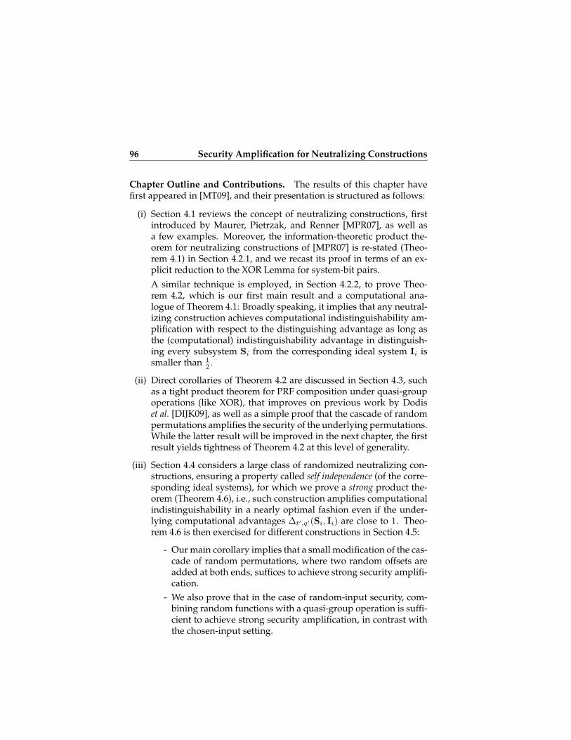
96 Security Amplification for Neutralizing Constructions
Chapter Outline and Contributions. The results of this chapter havefirst appeared in [MT09], and their presentation is structured as follows:
(i) Section 4.1 reviews the concept of neutralizing constructions, firstintroduced by Maurer, Pietrzak, and Renner [MPR07], as well asa few examples. Moreover, the information-theoretic product the-orem for neutralizing constructions of [MPR07] is re-stated (Theo-rem 4.1) in Section 4.2.1, and we recast its proof in terms of an ex-plicit reduction to the XOR Lemma for system-bit pairs.
A similar technique is employed, in Section 4.2.2, to prove Theo-rem 4.2, which is our first main result and a computational ana-logue of Theorem 4.1: Broadly speaking, it implies that any neutral-izing construction achieves computational indistinguishability am-plification with respect to the distinguishing advantage as long asthe (computational) indistinguishability advantage in distinguish-ing every subsystem Si from the corresponding ideal system Ii issmaller than 1
2 .
(ii) Direct corollaries of Theorem 4.2 are discussed in Section 4.3, suchas a tight product theorem for PRF composition under quasi-groupoperations (like XOR), that improves on previous work by Dodiset al. [DIJK09], as well as a simple proof that the cascade of randompermutations amplifies the security of the underlying permutations.While the latter result will be improved in the next chapter, the firstresult yields tightness of Theorem 4.2 at this level of generality.
(iii) Section 4.4 considers a large class of randomized neutralizing con-structions, ensuring a property called self independence (of the corre-sponding ideal systems), for which we prove a strong product the-orem (Theorem 4.6), i.e., such construction amplifies computationalindistinguishability in a nearly optimal fashion even if the under-lying computational advantages ∆t′,q′(Si, Ii) are close to 1. Theo-rem 4.6 is then exercised for different constructions in Section 4.5:
- Our main corollary implies that a small modification of the cas-cade of random permutations, where two random offsets areadded at both ends, suffices to achieve strong security amplifi-cation.
- We also prove that in the case of random-input security, com-bining random functions with a quasi-group operation is suffi-cient to achieve strong security amplification, in contrast withthe chosen-input setting.

4.1 Neutralizing Constructions 97
- Finally, in the case of chosen-input security, strong security am-plification can be achieved by adding a secret random offset tothe input. This improves on a previous construction by My-ers [Mye99, Mye03].
The results of this chapter are presented in the non-uniform setting only.The modifications to obtain uniform statements are fairly straightforward,and follow the same approach as in the proof of the uniform XOR Lemma(Theorem 3.19).
Related Work. The concept of a neutralizing construction was intro-duced by Maurer, Pietrzak and Renner [MPR07], allowing a unified treat-ment of indistinguishability amplification with respect to the information-theoretic distinguishing advantage. Previous results in this setting havebeen obtained by Vaudenay [Vau98, Vau99] within the framework of de-correlation theory.
In contrast, only limited work has addressed amplification resultswith respect to the computational distinguishing advantage. The firstproduct theorem is due to Luby and Rackoff [LR86], who proved thatthe cascade of two PRPs is strictly stronger than both of the individualcomponents. Yet, extensions of this result to longer cascades (as doneby Myers [Mye99]) only apply to constant-length cascades, due to thehigh complexity of the resulting reduction: This approach thus falls shortof proving amplification from a non-negligible advantage to a negligi-ble one, which is our ultimate goal. The first product theorem for PRFs(which follows as a corollary from Theorem 4.6) appeared in [Mye99](the result was subsequently published in [Mye03]). Only more recently,Dodis et al. [DIJK09] provided the first product theorem for PRFs via sim-ple XOR composition, which we improve quantitatively as an applicationof Theorem 4.2.
We additionally stress that our work on cascades is in contrast with aprevious line of work focusing on generic attacks against cascades [EG85,MM93, BR06, GM09a], where one only assumes black-box access to theunderlying block cipher, usually modeled as an ideal cipher.
4.1. Neutralizing Constructions
We start with the following definition, which differs slightly from the onegiven in [MPR07].

98 Security Amplification for Neutralizing Constructions
Definition 4.1. A construction C(·) is called neutralizing for system classesS1, . . . ,Sm and ideal systems I1, . . . , Im (with Ii ∈ Si for all i = 1, . . . ,m)if, for all S1, . . .Sm such that Si ∈ Si (for i = 1, . . . ,m), we have
C(S1, . . . ,Sm) ≡ C(I1, . . . , Im)
whenever there exists some i with Si ≡ Ii.
Neutralizing constructions capture the notion of a combiner [Her05]for computational indistinguishability properties: Whenever at least onesystem Si ∈ Si is computationally indistinguishable from Ii, then thesystems C(S1, . . . ,Sm) and C(I1, . . . , Im) are computationally indistin-guishable. Typical examples for the classes Si are the classes of randomvariables, random functions, and random permutations. Without loss ofgenerality, we assume that each such system class S satisfies the naturalproperty that if S ∈ S, then fixing (even partially) the random choices insome implementation of S yields a system in S as well. In particular, it isconvenient to say that C(·) is neutralizing for S1, . . . ,Sm and I1, . . . , Imif it is neutralizing for some classes S1, . . . ,Sm with Si ∈ Si and Ii ∈ Sifor i = 1, . . . ,m.
We provide two examples of neutralizing constructions with two sub-systems. (Both constructions extend naturally to an arbitrary number ofsubsystems.)
Example 4.1. Every quasi-group operation1 ? on a finite set Y induces aconstruction C(·) such that C(F,G) := F ?G which is neutralizing forany two random functions F and G : X → Y and ideal systems I and Jbeing independent URFs. In particular, I ? J is also a URF. As a specialcase, this result holds for random variablesX,Y overY , the ideal systemsbeing uniform random elements of Y .
Example 4.2. The cascade operator B induces a construction C′(·) withC′(Q1,Q2) := Q1 B Q2 which is neutralizing for any two cc-statelessrandom permutations Q1 and Q2 : X → X (in fact Q1 can possibly bestateful) where the ideal systems I and J are both URPs X → X . Inparticular, I B J is also a URP. If Q1 is cc-stateless, then the same resultholds even in the two-sided case for 〈Q1〉 and 〈Q2〉 (with ideal system〈P〉 for a URP P).
1That is, given a, c ∈ Y (or b, c ∈ Y) there exists a unique b (a) such that a ? b = c.An example is bit-wise XOR ⊕ for Y = 0, 1n, and any group operation is a quasi-groupoperation as well.

4.2 Product Theorem for Neutralizing Constructions 99
4.2. Product Theorem for Neutralizing Constructions
4.2.1. The Information-Theoretic Product Theorem
Throughout this and the following subsections, let C(·) be a neutraliz-ing construction for the real systems S1, . . . ,Sm and the correspondingideal systems I1, . . . , Im. We re-state (and give a proof in slightly differentterms) the general product theorem upper bounding the distinguishingadvantage ∆q(C(S1, . . . ,Sm),C(I1, . . . , Im)) in terms of the individualadvantages ∆qi(Fi, Ii), with qi being the number of queries C(·) makesto i-th subsystem when queried q times. The proof is illustrative for con-veying the main ideas underlying the proof of Theorem 4.2 below.
Theorem 4.1. Let C(·) be as above, and let q > 0 be such that C(·) makes qiqueries to its i-th subsystem when invoked q times. Then,
∆q(C(S1, . . . ,Sm),C(I1, . . . , Im)) ≤ 2m−1 ·m∏i=1
∆qi(Si, Ii).
Proof. The core of the proof is a generic argument (i.e. it holds for all dis-tinguishers) reducing the task of upper bounding the distinguishing ad-vantage ∆q(C(S1, . . . ,Sm),C(I1, . . . , Im)) for a neutralizing constructionC(·) to an instance of the XOR-lemma.2 Define
S := (S1, . . . ,Sm) and I := (I1, . . . , Im),
and let B a bit such that PB(0) = 12m−1 . It is easy to verify that for all
distinguishers D,
∆D(C(S),C(I)) = 2m−1 ·∆D(〈C(S),C(I)〉B ,C(I))
= 2m−1 ·∣∣∣GuessD(B′ | 〈〈C(S),C(I)〉B ,C(I)〉B′)
∣∣∣B′ is a uniform random bit, independent of B. Note that conditioned onB′ = 0, the system 〈〈C(S),C(I)〉B ,C(I)〉B′ behaves as C(S) with proba-bility 1
2m−1 , and as C(I) otherwise (i.e., with probability 1− 12m−1 ). On the
other hand, conditioned on B′ = 1 it always behaves as C(I). In particu-lar, this implies that (for independent uniform random bits B1, . . . , Bm),the following two system-bit pairs are equivalent
(〈〈C(S),C(I)〉B ,C(I)〉B′ , B′) ≡≡ (C(〈S1, I1〉B1
, . . . , 〈Sm, Im〉Bm), B1 ⊕ · · · ⊕Bm) ,
2This only appears implicitly in the information-theoretic product theorem of [MPR07].

100 Security Amplification for Neutralizing Constructions
because of the neutralizing property. We thus obtain
GuessD(B′ | 〈〈C(S),C(I)〉B ,C(I)〉B′) =
= GuessD(B1 ⊕ · · · ⊕Bm |C(〈S1, I1〉B1, . . . , 〈Sm, Im〉Bm))
= GuessDC(B1 ⊕ · · · ⊕Bm | 〈S1, I1〉B1‖ · · · ‖〈Sm, Im〉Bm)
≤ Guessq1,...,qm(B1 ⊕ · · · ⊕Bm | 〈S1, I1〉B1‖ · · · ‖〈Sm, Im〉Bm),
where we have “absorbed” the computation of C(·) into D, clearly with-out modifying the advantage. Using the (information theoretic) XORLemma (Theorem 3.13), we have
∆q(C(S),C(I)) ≤ 2m−1 ·m∏i=1
Guessqi(Bi | 〈Si, Ii〉Bi)
= 2m−1 ·m∏i=1
∆qi(Si, Ii).
A computational version of Theorem 4.1 seems easy to obtain, as wecan simply replace the use of the information-theoretic XOR lemma bythe computational one. Yet, a major issue is due to the presence of thefactor 2m−1: Namely, when using the computational XOR lemma, theadditive term γ is also multiplied by 2m−1, and the term 2m−1 · γ is gen-erally too large (or, in other words, in order to make it sufficiently small,the resulting γ would make the reduction inefficient). Below, we over-come this issue by considering the casem = 2 first, and subsequently usethis as an “Isolation Lemma” to obtain the full theorem.
4.2.2. The Computational Product Theorem
From now on, assume that all systems, except for possibly Sm and Imare cc-stateless. The computational version of Theorem 4.1 relies on thecanonical implementationA〈Si,Ii〉Bi of 〈Si, Ii〉Bi which chooses a randombit Bi ∈ 0, 1 and answers each query using the implementations ASi
and AIi (with respective complexities tASiand tAIi
) of Si or of Ii, re-spectively, depending on the value of Bi. It can be implemented withcomplexity tA〈Si,Ii〉Bi
(q, s) = maxtASi(q, s), tAIi
(q, s) + O(1). This alsoyields an implementation of (〈Si, Ii〉Bi , Bi) with the same complexity (byadditionally outputting the bit Bi). We let ϕ⊕ be as in Section 3.3.3, andfor all i, we denote li := sA〈Si,Ii〉Bi
(qi · ϕ⊕) and l<i :=∑i−1j=1 lj (for un-
derstood q1, . . . , qm−1). Finally, we let tACbe the time complexity of an
efficient implementation AC of C(·).

4.2 Product Theorem for Neutralizing Constructions 101
Theorem 4.2. For all t, q > 0 and γ > 0, if ∆t′i,q′i(Si, Ii) ≤ 1
2 for all i =1, . . . ,m− 1, then
∆t,q(C(S1, . . . ,Sm),C(I1, . . . , Im)) ≤ 2m−1 ·m∏i=1
∆t′i,q′i(Si, Ii) + 2γ,
where
t′i := l<i + ϕ⊕ ·[t+ tAC
(q) +O(i−1∑j=1
tA〈Sj ,Ij〉Bj(qj , lj)
+
m∑j=i+1
tA〈Sj ,Ij〉Bj(qj)
)]and q′i := ϕ⊕ · qi for all i = 1, . . . ,m− 1, whereas
t′m := l<m + t+ tC(q) +O
m−1∑j=1
tA〈Sj ,Ij〉Bj(qj , lj)
and q′m := qm.
In the remainder of this section, we provide a full proof of the theo-rem, whereas Section 4.3 presents some applications.
The key technique used in the proof of Theorem 4.2 is a version of theIsolation Lemma (Lemma 3.16) in the setting of computational indistin-guishability amplification. While this follows the same lines as the proofof Theorem 4.1 given above for the case m = 2, we rely on the strongerstatement given by the Isolation Lemma (Lemma 3.16) in order to provethe result for the most general setting where no additional structural re-quirements are made on the construction C(·).
ISOLATION LEMMA. For the sake of simplifying notation, for all i =1, . . . ,m, we denote as Ai := A〈Si,Ii〉Bi the implementation of the sys-tem 〈Si, Ii〉Bi . It is also convenient to write C(S1‖ . . . ‖Sm) instead ofC(S1, . . . ,Sm), i.e., we see the construction as accessing the parallel com-position of all subsystems, rather than the individual subsystems. Fur-thermore, we define (for i ≤ j) the shorthands
S[i,j] := Si‖ . . . ‖SjI[i,j] := Ii‖ . . . ‖Ij
A[i,j][σi, . . . , σj ] := Ai[σi]‖ · · · ‖Aj [σj ].
Also, let ϕisol be as in Section 3.3.4.

102 Security Amplification for Neutralizing Constructions
Lemma 4.3. Let i ∈ 1, . . . ,m − 1, let γ > 0, and let D ∈ Dt,q be a dis-tinguisher. Moreover, let σ1, . . . , σi−1 be valid states for A1, . . . , Ai−1, respec-tively, with |σj | ≤ lj (for j = 1, . . . , i− 1), and let b[1,i−1] ∈ 0, 1 be a binaryvalue. Also, assume that for a uniform bit B,
GuessD(b[1,i−1]⊕B |C(A[1,i−1][σ1, . . . , σi−1]‖〈S[i,m], I[i,m]〉B)) > 2δε+2γ.
Then, at least one of the following two statements is true:
(i) There exists a valid state σi for Ai with |σi| ≤ li and a bit b[1,i] ∈ 0, 1such that
GuessD(b[1,i] ⊕B |C(A[1,i][σ1, . . . , σi]‖〈S[i+1,m], I[i+1,m]〉B)) > δ;
(ii) There exists a distinguisher D′i ∈ Dt′i,q′i such that
∆D′i(Si, Ii) ≥ GuessD′i(Bi | 〈Si, Ii〉Bi) > ε,
and
t′i = l<i + ϕisol ·
t+ tAC(q) +O
i−1∑j=1
tAj (qj , lj) +
m∑j=i+1
tAj (qj)
and q′i = ϕisol · qi.
Proof. A straightforward calculation yields (for an additional uniformrandom bit B′ independent of B, and for A := A[1,i−1][σ1, . . . , σi−1])
GuessD(b[1,i−1] ⊕B |C(A‖〈S[i,m], I[i,m]〉B)) =
= 2 ·GuessD(b[1,i−1] ⊕B |C(A‖〈〈S[i,m], I[i,m]〉B′ , I[i,m]〉B)). (4.1)
Also, as C(·) is neutralizing for S1, . . . ,Sm and I1, . . . , Im, it is also neu-tralizing for 〈S1, I1〉B1 , . . . , 〈Si−1, Ii−1〉Bi−1 ,Si, . . . ,Sm and I1, . . . , Im. Inturn, because 〈S1, I1〉B1 , . . . , 〈Si−1, Ii−1〉Bi−1 are cc-stateless systems, theconstruction C(·) is also neutralizing forA1[σ1], . . . , Ai−1[σi−1],Si, . . . ,Smand I1, . . . , Im. This yields
C(A‖Si‖I[i+1,m]) ≡ C(A‖Ii‖S[i+1,m]) ≡ C(A‖I[i,m]) ≡ C(I1, . . . , Im),
from which we infer the equivalence
(C(A‖〈〈S[i,m], I[i,m]〉B′ , I[i,m]〉B), b[1,i−1] ⊕B) ≡≡ (C(A‖〈Si, Ii〉Bi‖〈S[i+1,m], I[i+1,m]〉B′′), b[1,i−1] ⊕Bi ⊕B′′) (4.2)

4.2 Product Theorem for Neutralizing Constructions 103
for independent uniform random bits Bi and B′′, since both system-bitpairs behave as C(I1, . . . , Im) whenever the bit is 1 − b[1,i−1], whereasotherwise they behave as C(I1, . . . , Im) or C(A‖S[i,m]) with probability1/2 each. Therefore, combining (4.1) and (4.2), the assumption of thelemma can equivalently be reformulated as
GuessDC(b[1,i−1] ⊕Bi ⊕B′′ |A|〈Si, Ii〉Bi‖〈S[i+1,m], I[i+1,m]〉B′) > δε+ γ,
We can now apply the Isolation Lemma (Lemma 3.16) to obtain the de-sired statement, and note that the running time to implement the system-bit pair (〈S[i+1,m], I[i+1,m]〉B′ , B′) is of the order
∑mj=i+1
tA〈Sj ,Ij〉Bj(qj) by
construction of A〈Sj ,Ij〉Bj .
FROM THE ISOLATION LEMMA TO THE PRODUCT THEOREM. For givent, q and γ, and γ := γ/(m−1), we let t′1, . . . , t′m and q′1, . . . , q′m be as in thestatement of Theorem 4.2, and define εi := ∆t′i,q
′i(Fi, Ii). Furthermore,
recall that εi ≤ 12 for all i = 1, . . . ,m− 1.
From now on, assume that Theorem 4.2 is false, and let D ∈ Dt,q bethe distinguisher such that
∆D(C(S1, . . . ,Sm),C(I1, . . . , Im)) = GuessD(B |C(〈F[1,m], I[1,m]〉B))
≥ 2m−1 · ε1 · · · εm + 2γ
for a uniform random bitB. Define γi := (m−1−i) ·γ for i = 0, . . . ,m−1and consider the statements STATi(σ1, . . . , σi, b) for a bit b ∈ 0, 1 andvalid states σ1, . . . , σi of A1, . . . , Ai respectively, with |σj | ≤ lj for j =1, . . . , i which holds if and only if
GuessD(b⊕B′ |C(A[1,i][σ1, . . . , σi]‖〈S[i+1,m], I[i+1,m]〉B′)) ≥≥ 2m−1−i · εi+1 · · · εm + γi
≥ 2 · εi+1 · (2m−1−(i+1) · εi+2 · · · εm + γi+1) + γ,
where we have used the facts that γi := γi−1 + γ and 2 · εi+1 ≤ 1.In particular, by our assumption STAT0(0) holds. Furthermore, givenSTATi(σ1, . . . , σi−1, b) holds for some i we apply the Isolation Lemma(Lemma 4.3). Note that condition (ii) cannot hold, as otherwise thereexists a distinguisher D′i such that ∆D′i(Si, Ii) > εi, but this contradictsthe assumed indistinguishability of Si and Ii, as we have defined εi withrespect to the maximal running time of a constructed distinguisher D′i.

104 Security Amplification for Neutralizing Constructions
Therefore, condition (i) must hold: In other words, we have shown thatfor all i = 0, . . . ,m− 2
STATi(σ1, . . . , σi, b) =⇒ ∃σi+1, b′ : STATi(σ1, . . . , σi, σi+1, b⊕ b′),
where all the states σ1, σ2, . . . are valid for their respective implementa-tions and are such that |σi| ≤ li. Iterating the argument we obtain thatthere exist σ1, . . . , σm−1 and a bit b such that
GuessD(b⊕Bm |C(A[1,m−1][σ1, . . . , σm−1]‖〈Sm, Im〉Bm)) >
> εm + γm−1 = εm.
Hence, the distinguisher
D′ := D(C(A[1,m−1][σ1, . . . , σm−1]‖·))⊕ b
obtains advantage larger than > εm, contradicting the assumed indistin-guishability of Sm and Im.
4.3. Applications of the Product Theorem
4.3.1. Sums of PRFs and Tightness
Let F1, . . . ,Fm : X → Y be random functions, with respective algorithmimplementations AFi , where all but Fm are required to be cc-stateless,and let ? be a quasi-group operation on Y . The operator ? is neutralizing,as discussed in Section 4.1, for F1, . . . ,Fm and ideal systems I1 = · · · =Im = R, where R : X → Y is a URF. We assume that elements of Y can beencoded using ` ≈ log |Y| bits. Recall that the canonical implementationof R keeps a linearly-growing state of size s = O(q ·`) after q queries, andanswers each query in time O(log(s)). Therefore, with tA〈Fi,R〉Bi
(q, s) =
O(maxtAFi(q, s), q · log(s+ q)) and li := O(maxsAFi
(ϕ⊕ · q), ϕ⊕ · q · `),we apply Theorem 4.2 to obtain the following result (we tacitly assumethat all advantages are bounded by 1
2 ):
Corollary 4.4. For all t, q > 0 and γ > 0,
∆t,q(F1 ? · · · ? Fm,R) ≤ 2m−1 ·m∏i=1
∆t′i,q′i(Fi,R) + 2γ.

4.3 Applications of the Product Theorem 105
We remark that the analogous result for PRGs follows as a specialcase, since a PRG can be seen as a one-input PRF.
A weaker version of this result was shown by Dodis et al. [DIJK09] forthe special case ? = ⊕: Their bounds depend in particular on the numberof queries, and is hence far away from our bound, which we prove to betight up to the additive term γ.
Remark 4.1 (Tightness). Consider the cc-stateless random function F thatbehaves as a URF R : 0, 1n → 0, 1n, with the exception that thefirst bit of F(0n) is one with probability 1
2 + ε.3 Note that ∆D(F,R) ≤ε for all D, as the function table of F has statistical distance ε from arandomly chosen function. However, on input 0n, the first output bit ofthe XOR F1⊕· · ·⊕Fm is one with probability 1
2 +2m−1εm: Therefore, theconstant-time distinguisher D∗ that returns the first output bit on input0n achieves advantage 2m−1εm.
Regardless of the security loss we are ready to accept, the bound inCorollary 4.4 is consequently tight up to the term γ, and Theorem 4.2cannot be improved at this level of generality.
4.3.2. Cascade of PRPs
Let P : 0, 1n → 0, 1n be a URP and let Q1, . . . ,Qm : 0, 1n →0, 1n be cc-stateless random permutations, where Qi and 〈Qi〉 are im-plemented by AQi
and A〈Qi〉, respectively. Recall that the B operatoris neutralizing for Q1, . . . ,Qm (all with ideal system P), as well as for〈Q1〉, . . . , 〈Qm〉 (all with ideal system 〈P〉). Recall that simulating theURP P (as well as the two-sided URP 〈P〉) requires the same complex-ity as implementing a URF. Therefore, similarly to the PRF case above,we have tA〈Qi,R〉Bi
(q, s) = O(maxtAQi(q, s), q · log(s + q)), as well as
li := O(maxsAQi(ϕ⊕ · q), ϕ⊕ · q · n) (and analogously for 〈Qi〉), and
Theorem 4.2 yields the following corollary:
Corollary 4.5. For all t, q > 0 and γ > 0,
∆t,q(Q1 B · · ·BQm,P) ≤ 2m−1 ·m∏i=1
∆t′i,q′i(Qi,P) + 2γ,
3This function is efficiently implementable by a stateful algorithm, whereas a keyedfunction approximating F can be built from any PRF: Just add sufficiently many bits tothe key to simulate the first output bit on input 0n, and behave otherwise as the originalPRF.

106 Security Amplification for Neutralizing Constructions
and
∆t,q(〈Q1〉B · · ·B 〈Qm〉, 〈P〉) ≤ 2m−1 ·m∏i=1
∆t′i,q′i(〈Qi〉, 〈P〉) + 2γ.
Furthermore, we note that Q1 is allowed to be stateful in the one-sided case, as Theorem 4.2 allows one system to be stateful: In fact, Bis not necessarily neutralizing whenever at least two permutations arestateful.
At time of publication (in [MT09]), this was the first result consider-ing two-sided PRPs, and even in the one-sided setting only the case m = 2was considered by Luby and Rackoff [LR86], and subsequently extendedto any constant m by Myers [Mye99]. (Also, a slightly weaker result forthe case m = O(log log n) is given in [Mye99].) However, all of these re-sults fall short of achieving security amplification, as they are not able totransform an ε-PRP for a non-negligible ε into a fully secure PRP. How-ever, contrary to the PRF case above, in this case the bound is not tight,and indeed we will show in Chapter 5 how it can be improved to achieveamplification well beyond advantage 1
2 .
4.4. A Strong Product Theorem
Since Theorem 4.2 holds for arbitrary neutralizing constructions, one can-not avoid the factor 2m−1 in the bound by Remark 4.1. This section showsa strong product theorem for subclass of neutralizing constructions sat-isfying a simple information-theoretic property, i.e., the obtained upperbound is roughly the product of the individual advantages. Contraryto Theorem 4.2, this result is not a computational analogue of an exist-ing information-theoretic statement: Instead, we take a proof-centric ap-proach, identifying properties that need to be satisfied by neutralizingconstruction C(·) in order to obtain a strong product theorem.
4.4.1. Self-Independence
We start with some intuition. For a neutralizing construction C(·) for cc-stateless systems S1, . . . ,Sm and I1, . . . , Im with ∆t′i,q
′i(Si, Ii) ≤ εi, we
want to prove that
∆t,q(C(S1, . . . ,Sm), I) ≤m∏i=1
εi + γ,

4.4 A Strong Product Theorem 107
where I := C(I1, . . . , Im). One possible proof approach, that we will fol-low, makes use of the isolation technique, as in the proof of Theorem 3.15:By a counting argument, it is not hard to show that given initial statess1, . . . , si−1 for S1, . . . ,Si−1 as well as a distinguisher D such that
∆D(C(S1(s1), . . . ,Si−1(si−1),Si, . . . ,Sm), I) >
m∏j=i
εj + γ
then either there exists si for Si such that
∆D(C(S1(s1), . . . ,Si(si),Si+1, . . . ,Sm), I) >
m∏j=i+1
εj + γ,
or, for a fraction εi of the si’s,
∆D(C(S1(s1), . . . ,Si(si),Si+1, . . . ,Sm), I) = ∆DCi(Si(si), Ii) > γ
where (recall that C(·) is neutralizing)
Ci(·) := C(S1(s1), . . . ,Si−1(si−1), ·,Si+1, . . . ,Sm).
In the latter case, we would like to build a distinguisher D′i out of Di :=DCi which contradicts indistinguishability of Si and Ii. The simpleststrategy is to let independent instances of Di sequentially interact withthe given system T, resulting in output bits b1, b2, . . ., where either T =Si(si) for some state si or T = Ii, producing an estimate p of the proba-bility P [Di(T) = 1] as the average of the bits b1, b2, . . .: If p is sufficientlyfar from P [Di(Ii) = 1] (say at least γ/2), then D′i outputs 1, otherwise itoutputs 0. It is not hard to verify that if the estimate is within an errorof at most γ/2 from the actual probability, D′i achieves advantage largerthan εi.4
Note that T = Si(si) is stateless, and hence the bits b1, b2, . . . are inde-pendent when interacting with T: By Hoeffding’s inequality (Lemma 2.1),p is indeed a good estimate of P [D(Ci(Si(si))) = 1]. However, in the casewhere T = Ii, the bi’s are not necessarily independent, and hence no state-ment about the quality of p can be made in general.
We introduce a condition which is sufficient for (almost) indepen-dence to be achieved, which we refer to as self-independence of an ideal
4This is because it outputs 1 on the εi-fraction of the si’s considered above, and outputs0 when interacting with Ii.

108 Security Amplification for Neutralizing Constructions
system I under a construction C(·): It captures the property that a com-putationally unbounded distinguisher is unable to tell apart the scenariowhere the same instance of I is accessed through independent instancesof C(·) from the setting where each instance of C(·) accesses an indepen-dent instance of I. Should Ci(·) satisfy this property for Ii above, then itwould be easy to show that a good estimate is produced also in the caseT = Ii.
Definition 4.2. The system I is η-self-independent under C(·) for a functionη : N×N→ R≥0, if for all q, λ > 0, the best (information-theoretic) distin-guishing advantage when allowing q queries to each subsystem satisfies
∆q,...,q(C1(I)‖ . . . ‖Cλ(I),C1(I1)‖ . . . ‖Cλ(Iλ)) ≤ η(q, λ),
where C1(·), . . . ,Cλ(·) and I1, . . . , Iλ are independent copies of C(·) andI, respectively.
As an example, consider the construction C(·) which generates a (se-cret) random n-bit offset Z, and given access to a random function F :0, 1n → 0, 1n, C(F) returns F(x ⊕ Z) upon each query x. It is nothard to show that a URF R : 0, 1n → 0, 1n is η-self-independent un-der C(·) for η(q, λ) ≤ q2λ2
2 · 2−n, i.e., the probability that for some distincti 6= j the instances Ci(·) and Cj(·) invoke R with the same input.
4.4.2. A Product Theorem from Self-Independence
In the following, let C(·) be a neutralizing construction for the real sys-tems S1, . . . ,Sm and ideal system I1, . . . , Im, all of which (with the pos-sible exception of Sm and Im) are cc-stateless. Furthermore, we assumethat Si(·) is efficiently implementable for all i = 1, . . . ,m − 1,5 and thecorresponding (short) random variable Si is drawn from the set Si. Also,we let E(·) be a construction restricting access to Si and Ii, in the senseof Section 2.6.3. Finally, for i = 1, . . . ,m, and for s1 ∈ S1, . . . , si−1 ∈ Si−1
we define
C(i)s1,...,si−1
(·) := C(S1(s1), . . . ,Si−1(si−1), · ,Si+1, . . . ,Sm)
and consider the following two properties:5While the same techniques as in the proof of Theorem 3.15 could be used to address
general cc-stateless systems where Si(·) is not necessarily efficient, this will not be neces-sary for our applications: In particular, for the application for Theorem 4.2, we always needto consider systems with no such efficient implementations, such as URFs and URPs, butthis is not needed.

4.4 A Strong Product Theorem 109
(i) For all i = 1, . . . ,m− 1 (the property is not necessary for i = m) andall s1 ∈ S1, . . . , si−1 ∈ Si−1, the ideal system Ii is η-self-independentunder the construction C
(i)s1,...,si−1(·) for some small function η.
(ii) For all i = 1, . . . ,m and s1 ∈ S1, . . . , si−1 ∈ Si−1, there exists aconstruction T
(i)s1,...,si−1(·) with the property that for independent
instances T1(·), . . . ,Tλ(·) and C1(·), . . . ,Cλ(·) of T(i)s1,...,si−1(·) and
C(i)s1,...,si−1(·), respectively, and all compatible systems S,
T1(E(S))‖ · · · ‖Tλ(E(S)) ≡ C1(S)‖ · · · ‖Cλ(S).
We define tTi as the maximal complexity (taken over all s1, . . . , si−1)for implementing the construction T
(i)s1,...,si−1(·).
In the following, we define λ :=(
4mγ
)2
· ln(
4mγ
), for understood m and
γ.
Theorem 4.6. Let q > 0, C(·), and E(·) be as above satisfying conditions (i)and (ii), and assume that upon q queries, C(·) makes at most qi queries to thei-th subsystem. Then, for all t > 0 and γ > 0,
∆t,q(C(S1, . . . ,Sm),C(I1, . . . , Im)) ≤m∏i=1
∆t′i,q′i(E(Si),E(Ii))
+
m−1∑i=1
η(qi, λ) + γ,
wheret′i := λ · (t+O(tTi(qi))) and q′i := λ · qi
for all i = 1, . . . ,m− 1, whereas t′m := t+O(tTm(q)) and q′m := qm.
The full proof of Theorem 4.6 is deferred to Section 4.4.3. Further-more, in Section 4.5 we provide application examples of Theorem 4.6.
4.4.3. Proof of the Strong Product Theorem
This section presents a proof of Theorem 4.6. As in the cases of The-orems 3.15 and 4.2, the proof is based on the isolation technique. Itabstracts and generalizes the proof technique used by Myers [Mye03]

110 Security Amplification for Neutralizing Constructions
(which was in turn based on Levin’s proof of the XOR-lemma [Lev87,GNW95]). Throughout this section, we let
S[i,j] := Si, . . . ,Sj ,
S[i,j](si, . . . , sj) := Si(si), . . . ,Sj(sj),
I[i,j] := Ii, . . . , Ij .
THE ISOLATION LEMMA. In the following, we let I := C(I1, . . . , Im) and
define λ = λ(m, γ) :=(
4γ
)2
· ln(
4γ
). Also, in the following, let λ be de-
fined as above with respect to some understood γ, whereas with respect
to γ we define λ :=(
4γ
)2
· ln(
4γ
).
Lemma 4.7. Let i ∈ 1, . . . ,m− 1, ζ > 0, and γ > 0. Assume that D makesq queries to C(·) resulting in qj queries to each of them subsystems Sj , and thatfor values s1 ∈ S1, . . . , si−1 ∈ Si−1 we have
P[D(C(S[1,i−1](s1, . . . , si−1),S[i,m])) = 1
]− P [D(I) = 1] > δ · ε+ ζ + γ,
then at least one of the two following statements holds:
(i) There exists a value si ∈ Si such that
P[D(C(S[1,i](s1, . . . , si),S[i+1,m]) = 1]−P[D(I) = 1] > δ+ζ−η(qi, λ).
(ii) There exists a distinguisher D′i such that ∆D′i(E(Si),E(Ii)) > ε whichmakes q′i := λ · qi queries and has time complexity t′i := λ · (t+ tTi(q)).
FROM THE ISOLATION LEMMA TO THEOREM 4.6. Similarly to the casesof Theorems 3.15 and 4.2, we apply the isolation lemma iteratively toobtain Theorem 4.6. Fix t, q, γ > 0 (and let γ := γ/(m − 1)) such thatupon q queries C(·) makes q1, . . . , qm queries to its subsystems. For alli = 1, . . . ,m, let t′i, q
′i as in the statement of Theorem 4.6, and let εi :=
∆t′i,q′i(Si, Bi).
Assume towards a contradiction that there exists a distinguisher Dwith running time t making q queries to C such that
∆D(C(S[1,m]), I) ≥ P[D(C(S[1,m])) = 1
]− P [D(I) = 1]
≥ ε1 · · · εm +
m−1∑i=1
η(qi, λ) + γ.

4.4 A Strong Product Theorem 111
and define γi := (m − 1 − i) · γ for i = 0, . . . ,m − 1 and consider thestatements STATi(s1, . . . , si) which holds if and only if
P[D(C(S[1,i](s1, . . . , si),S[i+1,m])) = 1
]− P [D(I) = 1] ≥
≥ εi+1 · · · εm +
m−1∑j=i+1
η(qj , λ) + γi
≥ εi+1 · (εi+2 · · · εm + γi+1) +
m−1∑j=i+1
η(qj , λ) + γ.
In particular, by our assumption STAT0 holds. By the Isolation Lemma(Lemma 4.7) and the fact that ∆t′i+1,q
′i+1
(Si+1, Ii+1) ≤ εi+1, whenever thecondition STATi(s1, . . . , si) holds for some s1, . . . , si, then condition (ii)cannot hold, and hence condition (i) must hold, i.e., there must exists si+1
such that STATi+1(s1, . . . , si+1) holds. In other words, we have shownthat for all i = 0, . . . ,m− 2
STATi(s1, . . . , si) =⇒ ∃si+1 : STATi+1(s1, . . . , si+1).
Iterating the argument we obtain that there exist s1, . . . , sm−1 such thatSTATm−1(s1, . . . , sm−1) holds, i.e.
P[D(C(S[1,m−1](s1, . . . , sm−1),Sm) = 1]− P[D(I) = 1] ≥ εm.
This, however, gives rise to a distinguisher D′m := D(Tm−1,s1,...,sm−1(·))
with advantage εm and the given complexity t′m, contradicting the indis-tinguishability assumption on Sm and Im.
PROOF OF THE ISOLATION LEMMA (LEMMA 4.7). We fix i ∈ 1, . . . ,mas in the statement of the lemma. It is convenient to denote η := η(qi, λ),as well as C(i)(·) := C
(i)s1,...,si−1(·). Note that since C(·) is neutralizing,
we have C(i)(Ii) ≡ I. Furthermore, we also define the function α : Si →[−1, 1] such that
α(s) := P[D(C(i)(S(s))) = 1]− P[D(I) = 1].
Clearly, by the assumption of the lemma, we have E[α(Si)] > δ · ε+ ζ+γ.Furthermore, if there existed an si such that α(si) > δ + ζ − η, the firststatement of the lemma would be directly true. Therefore, we assume inthe following that α(s) ≤ δ+ ζ − η for all s ∈ Si. Moreover, we define theset
G := s ∈ Si |α(s) > γ/2.

112 Security Amplification for Neutralizing Constructions
Distinguisher D′i:// for S ∈ E(Si),E(Ii)
for j := 1, . . . , λ dooj := D(T
(i)s1,...,si−1(S))
o := 1λ ·∑λj=1 oj
if o− π > γ/4 thenreturn 1
elsereturn 0
Distinguisher D′′i :// for S ∈ Si, Ii
for j := 1, . . . , λ dooj := D(C(i)(S))
o := 1λ ·∑λj=1 oj
if o− π > γ/4 thenreturn 1
elsereturn 0
Figure 4.1: Distinguishers D′i and D′′i in the proof of Lemma 4.7. In bothcases, π equals P[D(I) = 1].
The following claim gives a lower bound on the probability that Si is inthe set G.
Claim 5. P[Si ∈ G] > ε+ η + γ/2.
Proof. Assume, towards a contradiction, that P[Si ∈ G] ≤ ε + γ/2 + η.Then,
E[α(Si)] = P[Si ∈ G] · E[α(Si)|Si ∈ G] + P[Si /∈ G] · E[α(Si)|Si /∈ G]
≤ (ε+ η + γ/2) · (δ + ζ − η) + γ/2
≤ εδ + ζ − η + η + γ/2 + γ/2 = εδ + ζ + γ.
which is in contradiction with the assumption on D.
We construct the distinguisher D′i for distinguishing E(Si) from E(Ii)as specified on the left-hand-side of Figure 4.1: With π := P[D(I) = 1],D′i simulates λ independent instances of D(T
(i)s1,...,si−1(·)) sequentially in-
teracting with the given system S, and computes the average o of the λbits output by these instances, and finally outputs 1 if o > π + γ/4, and0 otherwise. Note that by the property of T(i)
s1,...,si−1 we can equivalentlyconsider a distinguisher D′′i for Si and Ii (depicted on the right-hand-side of Figure 4.1) which computes the bits o1, . . . , oλ by letting inde-pendent instances of D(C(i)(·)) interact with the given system. Clearly,∆D′i(E(Si),E(Ii)) = ∆D′′i (Si, Ii), and we thus focus on the latter advan-tage.
The remainder of the proof consists of the following two lemmas.

4.4 A Strong Product Theorem 113
Lemma 4.8. P[D′′i (Si(s)) = 1] > 1− e−λ(γ/4)2
for all s ∈ G.
Lemma 4.9. P[D′′i (Ii) = 1] ≤ e−λ(γ/4)2
+ η(qi, λ).
Before we turn to the proofs of the two lemmas, we note that theysuffice to obtain the isolation lemma, since by Claim 5
∆D′′i (Si, Ii) ≥ P[Si ∈ G] · P[D′′i (Si(Si)) = 1|Si ∈ G]− P[D′′i (Ii) = 1]
> (ε+ γ/2 + η)(1− e−λ(γ/4)2
)− e−λ(γ/4)2 − η≥ ε+ γ/2 + η − 2e−λ(γ/4)2 − η = ε+ γ/2− 2e−λ(γ/4)2
= ε
for the chosen value of λ.
Proof of Lemma 4.8. Since the system Si(s) is stateless, note that for a fixeds ∈ G the random variables o1, . . . , oλ are independent binary variableswith
p(s) := P[oj = 1] = P[D(C(i)(Si(s))) = 1],
and thus E[o] = p(s). We know that p(s)− π > γ/2, since s ∈ G, and thuso−π ≤ γ/4 implies that o < p(s)−γ/4. Therefore, by Hoeffding’s bound,we have
P[D′′i (Si(s)) = 0] = P[o− π ≤ γ/4] ≤ P[o < p(s)− γ/4] < e−λ(γ/4)2
.
Proof of Lemma 4.9. Consider a distinguisher D′′i which given access to
the parallel composition S1‖ . . . ‖Sλ of λ systems S1, . . . ,Sλ, computesoj := D(Sj) for all j = 1, . . . , λ, and then outputs its decision bit as D′′i .Clearly, for independent instances C(i)
1 (·), . . . ,C(i)λ (·) of C(i)(·) we have
P[D′′i (Ii) = 1] = P[D′′i (C
(i)1 (Ii)‖ . . . ‖C(i)
λ (Ii)) = 1],
i.e., where every system in the parallel composition accesses the sameinstance Ii. Note that because of the η-self-independence of Ii under C(i)
we have, for independent instances Ii,1, . . . , Ii,λ of Ii
∆D′′i (C
(i)1 (Ii)‖ . . . ‖C(i)
λ (Ii),C(i)1 (Ii,1)‖ . . . ‖C(i)
λ (Ii,λ)) ≤ η(qi, λ),
from which we directly infer
P[D′′i (Ii) = 1] ≤ η(qi, λ) + P[D′′i (C
(i)1 (Ii,1)‖ . . . ‖C(i)
λ (Ii,λ)) = 1]. (4.3)

114 Security Amplification for Neutralizing Constructions
We hence upper bound the probability on the right-hand side. Notethat, in this case, the variables o1, . . . , oλ are assigned independent equally-distributed values, with P[oj = 1] = π all j = 1, . . . , λ (by the neutralizingproperty of C(·)), and thus E[o] = π holds as well. Then, by Hoeffding’sinequality,
P[D′′i (C
(i)1 (Ii,1)‖ . . . ‖C(i)
λ (Ii,λ)) = 1] = P[o− π > γ/4] < e−λ·(γ/4)2
,
which combined with (4.3) yields the desired upper bound.
4.5. Applications of the Strong Product Theorem
This section presents some applications of Theorem 4.6. Throughout thissection, let Q1, . . . ,Qm : 0, 1n → 0, 1n be cc-stateless random per-mutations, and let F1, . . . ,Fm : 0, 1n → 0, 1` be cc-stateless randomfunctions. In particular, we let Qi ≡ Qi(Si) for some random variable Siover a set Si, for all i = 1, . . . ,m, and analogously we have Fi ≡ Fi(Si).Furthermore, let P : 0, 1n → 0, 1n and R : 0, 1n → 0, 1` be aURP and URF, respectively. Assume that Qi(s)(x) (and Q−1
i (s)(y)) andFi(s)(x) can be computed in time tQi and tFi , respectively, for all s, x,and y.
4.5.1. Randomized Cascade of PRPs
Our first application is a strong product theorem for (two-sided) PRPs.We modify the (two-sided) cascade 〈Q1〉 B · · · B 〈Qm〉 by choosing twoindependent random offsets that are added to the inputs and the outputs,i.e., we consider 〈⊕Z1
〉B 〈Q1〉B · · ·B 〈Qm〉B 〈⊕Z2〉 for two independent
uniform n-bit strings Z1, Z2, where for some z ∈ 0, 1n the system 〈⊕z〉is the two-sided mapping which answers a forward query (x,+) withx ⊕ z and a backward query (y,−) with y ⊕ z. The computational over-head is minimal compared to the regular cascade, and requires only ad-ditional storage for two n-bit strings (which are to be seen as part of thesecret key).6 Clearly the neutralizing property of the original cascade ispreserved.
The central observation is that the two additional random offsets en-sure property (i) and allow for applying Theorem 4.6. More formally,for some i ∈ 1, . . . ,m and s1 ∈ S1, . . . , si−1 ∈ Si−1 we define (for a
6The idea of adding random offsets at both ends of a permutation was already used byEven and Mansour [EM97], though in a completely different context.

4.5 Applications of the Strong Product Theorem 115
system S implementing a two-sided permutation from n bits to n bits)the construction N(·) as choosing two offsets Z1, Z2 independently anduniformly at random, as well as Si+1, . . . , Sm, and such that
N(S) := 〈⊕Z1〉B 〈Q1(s1)〉B · · ·B 〈Qi−1(si−1)〉B S
B 〈Qi+1(Si+1)〉B · · ·B 〈Qm(Sm)〉B 〈⊕Z2〉.
The following lemma states the self-independence of a (two-sided) URP〈P〉 under N(·).
Lemma 4.10. Let N1(·), . . . ,Nλ(·) be independent instances of N, and letP1, . . . ,Pλ,P : 0, 1n → 0, 1n be independent URPs. Then
∆q,...,q(N1(〈P〉)‖ · · · ‖Nλ(〈P〉),N1(〈P1〉)‖ · · · ‖Nλ(〈Pλ〉)) ≤ λ2 · q2 · 2−n.
In other words, 〈P〉 is η-self-independent under N(·) for η(q, λ) := λ2q22−n.
Proof. For notational simplicity, we define two systems H0 and H1 withMBOs such that
H−0 := N1(〈P〉)‖ · · · ‖Nλ(〈P〉) and H−1 := N1(〈P1〉)‖ · · · ‖Nλ(〈Pλ〉).
For both systems, all t = 1, . . . , λ, and all i ≥ 1, letX (t)i contain those n-bit
strings x for which, when processing the first i queries, Nt(·) has issueda forward query (x,+), or alternatively a backward query (y,−) of Nt(·)was answered with the value x by the given permutation. Analogously,let Y(t)
i contain those n-bit strings y for which when processing the first iqueries Nt(·) has issued a backward query (y,−), or alternatively a for-ward query (x,+) of Nt(·) was answered by y.
For both systems H0 and H1, the respective MBOs A1, A2, . . . andB1, B2, . . . are such that Ai = 1 (or Bi = 1) if for some t 6= t′ we haveX (t)i ∩ X
(t′)i 6= ∅ or Y(t)
i ∩ Y(t′)i 6= ∅.
We note that for all i ≥ 1,
pH0
Yi|XiY i−1Ai=0 = pH1
Yi|XiY i−1Bi=0,
because for both systems, if the MBO is 0, the query to 〈P〉 / 〈Pt〉 as-sociated with a (fresh) forward query to Nt(〈P〉) / Nt(〈Pt〉) returns auniform value from 0, 1n \⋃t′ Y(t)
i−1. (The case of a backward query issymmetric.) Furthermore,
pH0
Ai=0|XiY i−1Ai−1=0 ≥ pH1
Bi=0|XiY i−1Bi−1=0

116 Security Amplification for Neutralizing Constructions
because, for system H0, the condition X (t)i ∩ X
(t′)i = ∅ holds for all t 6= t′
if and only if Y(t)i ∩ Y
(t′)i = ∅ for all t 6= t′. Therefore, by Lemma 2.6, we
obtain∆D(H−0 , H
−1 ) ≤ νD(H1)
for any distinguisher D issuing at most q queries to each subsystem (andthus making totally at most λ · q queries).
We thus focus on upper bounding the probability νD(H1) that D pro-vokes Bλ·q = 1. More specifically, let Z(t)
1 , Z(t)2 , S
(t)i+1, . . . , S
(t)m be the val-
ues taken byZ1, Z2, Si+1, . . . , Sm in Nt(·) for t = 1, . . . , λ. Note that for allvalues z(t)
1 , z(t)2 and s(t)
i+1, . . . , s(t)m taken by these variables, the system H1
behaves as the parallel composition of λ independent (two-sided) ran-dom permutations. We can thus apply Lemma 2.9. We assume that weare given input-output pairs (u
(t)1 , v
(t)1 ), . . . , (u
(t)q , v
(t)q ) for Nt(〈Pt〉) for
t = 1, . . . , λ, i.e., the i-th query to Nt(〈Pt〉) has been either a forwardquery u
(t)i with output v(t)
i or a backward query v(t)i with output u(t)
i .Moreover, we define for all i = 1, . . . , q and t = 1, . . . , λ
P(t)i :=
(Q1(s1) B · · ·BQi−1(si−1)
)(u
(t)i ⊕ Z
(t)1 )
Q(t)i :=
(Q−1m (S(t)
m ) B · · ·BQ−1i+1(S
(t)i+1)
)(v
(t)i ⊕ Z
(t)2 ),
i.e., these are the corresponding input-output pairs for the underlyingpermutations 〈P1〉, . . . , 〈Pλ〉. Note that all of these random variables are(individually) uniformly distributed and furthermore, given t 6= t′, i, jwe have P[P
(t)i = P
(t′)j ] = 2−n and P[Q
(t)i = Q
(t′)j ] = 2−n. Therefore,
Bλq = 1 implies that there exist distinct t, t′ and (not necessarily distinct)i, j such that P (t)
i = P(t′)j or Q(t)
i = Q(t′)j . By the union bound we con-
clude that
νD(H1) ≤ 2 ·(λ
2
)· q2 · 2−n ≤ λ2 · q2 · 2−n.
Therefore, we can combine Theorem 4.6 (with E(·) being the identity)and Lemma 4.10 to obtain the following result.
Corollary 4.11. For all t, q, γ > 0, and independent uniform n-bit stringsZ1, Z2,
∆t,q(〈⊕Z1BQ1 B · · ·BQm B⊕Z2
〉, 〈P〉) ≤m∏i=1
∆t′i,q′i(〈Qi〉, 〈P〉)
+mq2λ2
2n+ γ,

4.5 Applications of the Strong Product Theorem 117
where t′i := λ ·(t+O(q ·∑j 6=i tQj )
)and q′i := λ · q for all i = 1, . . . ,m− 1,
whereas t′m := t+O(q ·∑m−1j=1 tQj ) and q′m := q.
The result can be used to obtain am (εm+ ν)-two-sided PRP from anyε-two-sided PRP, for a negligible function ν. (Note that the η-dependentterm is negligible for polynomial t, q and any γ which is the inverse of apolynomial.) It can be shown that the second random offset Z2 is super-fluous in the one-sided case.
4.5.2. Sum of Random-Input PRFs
The construction K(F1⊕· · ·⊕Fm) (i.e. the XOR of the functions accessedin a random-input attack) is clearly neutralizing (the ideal system beingK(R)). However, the fact that F1⊕· · ·⊕Fm and R are invoked on randominputs only allows for proving a much stronger result using Theorem 4.6,since it satisfies property (i) needed by the theorem.
More precisely, let us fix i ∈ 1, . . . ,m and s1 ∈ S1, . . . , si−1 ∈ Si−1,and define for a random function S : 0, 1n → 0, 1` the constructionW(·) as
W(S) := K(F1(s1)⊕ · · · ⊕ Fi−1(si−1)⊕ S⊕ Fi+1 ⊕ · · · ⊕ Fm).
Then, we can show the following.
Lemma 4.12. Let R,R1, . . . ,Rλ : 0, 1n → 0, 1` be independent URFs,and let W1(·), . . . ,Wλ(·) be independent instances of W(·), then
∆q,...,q(W1(R)‖ · · · ‖Wλ(R),W1(R1)‖ · · · ‖Wλ(Rλ)) ≤ q2λ2
22−n.
In other words, the URF R is η-self-independent under W for η(q, λ) ≤ q2λ2
2 ·2−n.
Proof. Consider the system H0 with an MBO A1, A2 . . . such that
H−0 := W1(R)‖ · · · ‖Wλ(R).
Each query i to the subsystem t is associated with a random input ri,t atwhich the XOR is evaluated, and let Ai := 0 if within the first i queriesthere exists no two random inputs rj,t = rk,t′ for distinct t 6= t′. Moreover,let H1 := W1(R1)‖ · · · ‖Wλ(Rλ).

118 Security Amplification for Neutralizing Constructions
As long as Ai = 0 holds in H0, the random function R is never eval-uated at the same input by two constructions Wt(·) and Wt′(·), andthus as long as Ai is 0, the system H0 behaves as H1: Corollary 2.7 andLemma 2.8 imply that for all distinguishers D issuing at most q queriesto each of the λ subsystems we have
∆D(H−0 ,H1) ≤ νD(H0) ≤(λ
2
)q22−n.
Moreover, for all i and keys s1 ∈ S1, . . . , si−1 ∈ Si−1, the appropri-ate construction T
(i)s1,...,si−1(·) generates random keys Si+1, . . . , Sm and
whenever invoked, it issues a query to K(S), obtaining (r, y), and out-puts the pair
(r,
i−1⊕j=1
Fj(sj)(r)⊕ y ⊕m⊕
j=i+1
Fj(Sj)(r)).
It is easy to see that these constructions satisfy property (ii), since K(·)evaluates the given function at a fresh random input upon each invoca-tion. Therefore, Theorem 4.6 yields the following result.
Corollary 4.13. For all t, q, γ > 0,
∆t,q(K(F1 ⊕ · · · ⊕ Fm),K(R)) ≤m∏i=1
∆t′i,q′i(K(Fi),K(R))
+(m− 1)q2λ2
2n+1+ γ,
where t′i := λ(t + O(q ·∑j 6=i tFj )
)and q′i := λ · q for all i = 1, . . . ,m − 1,
whereas t′m := t+O(q ·∑m−1j=1 tFj ) and q′m := q.
The result holds for any other quasi-group operation. It is remark-able that XOR satisfies much stronger indistinguishability amplificationproperties under random-input attacks than under chosen-input attacks.
4.5.3. Randomized XOR of PRFs
The first product theorem for PRFs, due to Myers [Mye03], consideredthe neutralizing composition Z1(F1) ⊕ · · · ⊕ Zm(Fm) for independentinstances of Z(·) (which we assume to be instantiated with ⊕, but any

4.5 Applications of the Strong Product Theorem 119
other quasi-group operation would work). We show that this result isimplied by Theorem 4.6. In fact, the same result holds for the constructionZ(F1 ⊕ · · · ⊕ Fm) using the same offset for all invocations.
More precisely, fix i ∈ 1, . . . ,m and s1 ∈ S1, . . . , si−1 ∈ Si−1, anddefine the constructions M(·) and M′(·) such that for any random func-tion S : 0, 1n → 0, 1`,
M(S) := Z(F1(s1)⊕ · · · ⊕ Fi−1(si−1)⊕ S⊕ Fi+1 ⊕ · · · ⊕ Fm
).
and
M′(S) := Z1(F1(s1))⊕ · · · ⊕ Zi−1(Fi−1(si−1))⊕ Zi(S)
⊕ Zi+1(Fi+1)⊕ · · · ⊕ Zm(Fm)),
Lemma 4.14. Let R,R1, . . . ,Rλ : 0, 1n → 0, 1` be independent URFs,and let M1(·), . . . ,Mλ(·) be independent instances of M(·), then
∆q,...,q(M1(R)‖ · · · ‖Mλ(R),M1(R1)‖ · · · ‖Mλ(Rλ)) ≤ q2 · λ2
4· 2−n
and
∆q,...,q(M1(R)‖ · · · ‖Mλ(R),M1(R1)‖ · · · ‖Mλ(Rλ)) ≤ q2 · λ2
4· 2−n.
In other words, the URF R is η-self-independent under M(·) and M′(·) forη(q, λ) ≤ q2λ2
2 · 2−n.
Proof. We just prove the statement for M(·), as the proof for M′(·) is fullyanalogous. We define the system H0 with MBO A1, A2, . . . such that
H−0 := M1(R)‖ · · · ‖Mλ(R)
To define the MBO, let Z1, . . . , Zλ be the random offsets chosen by Z(·)in M1, . . . ,Mλ, respectively: We let Ai := 0 if and only if among thefirst i queries there exists no two queries Xj , Xk, j 6= k to distinct sub-systems t, t′ ∈ 1, . . . , λ such that Xi ⊕ Zt = Xj ⊕ Zt′ , and Ai := 1otherwise. Clearly, as long as this does not hold, every query (regardlessof the systems) returns an independent random output, i.e., behaves asH1 := M1(R1)‖ · · · ‖Mλ(Rλ), and it is easy to verify that we can applyboth Corollary 2.7 and Lemma 2.8, and for all distinguishers D issuing atmost q queries to each of the λ subsystems we have
∆D(H−0 ,H1) ≤ maxxλq
pH0
Aλq|Xλq (1, xλq),

120 Security Amplification for Neutralizing Constructions
where xλq is a sequence of queries with q queries to each subsystem, andfor each such sequence and for each pair of systems t 6= t′ there are atmost q2 pairs of possibly colliding queries Xi ⊕ Zt, Xj ⊕ Zt′ , and theprobability that they collide is exactly 2−n. By the union bound we have
pH0
Aλq|Xλq (1, xλq) ≤
(λ
2
)· q2 · 2−n.
A major advantage of Myers’ original construction (which was un-observed so far) is that independent instances of the construction can besimulated even when only given access to Z(S) (with S ∈ Fi,R). Therelevance of this observation is due to the fact that the best advantageunder Z(·) can be significantly smaller than under direct access: Con-sider e.g. a good PRF which is modified to have the additional propertyof outputting the zero string when evaluated at some fixed known input,regardless of the key.
In order to apply Theorem 4.6, the construction T(i)s1,...,si−1(·) chooses
independent instances Fi+1, . . . ,Fm, Z1(·), . . . ,Zi−1(·),Zi+1(·), . . . ,Zm(·),and a random n-bit string Z, and on input x queries x ⊕ Z to Z(S), ob-taining y ∈ 0, 1`, and outputs
y ⊕i−1⊕j=1
Zj(Fj(sj))(x)⊕m⊕
j=i+1
Zj(Fj)(x),
where Zj(Fj)(x) is the result of invoking the system Zj(Fj) on input x.Once again, condition (ii) is easily verified by the fact that access
through Z(·) can be re-randomized by simply adding a fresh random off-set to all inputs. Thus, Theorem 4.6 yields the following strengthenedversion of the main result of [Mye03].
Corollary 4.15. Let Z1(·), . . . ,Zm(·) be independent instances of Z(·). For allt, q, γ > 0,
∆t,q(Z1(F1)⊕ · · · ⊕ Zm(Fm),R) ≤m∏i=1
∆t′i,q′i(Z(Fi),Z(R))
+(m− 1)q2λ2
2n+1+ γ,
where t′i := λ(t + O(q ·∑j 6=i tFj )
)and q′i := λ · q for all i = 1, . . . ,m − 1,
whereas t′m := t+O(q ·∑m−1j=1 tFj ) and q′m := q.

Chapter 5
Security Amplification via ExtractingConstructions
Despite the generality of the results of Chapter 4, Theorem 4.2 only yieldsa mild form of advantage amplification, whereas Theorem 4.6 impliesoptimal amplification for a restricted class of randomized constructionsonly. Therefore, there exist examples, such as the (plain) cascade, forwhich only Theorem 4.2 applies, although one hopes for better bounds.To bridge this gap, this chapter introduces a class of constructions – calledextracting constructions – for which we prove a strong computational in-distinguishability amplification theorem.
Our paradigm is best illustrated by considering two finite randomvariables X and Y with statistical distance d(X,Y ) = ε. By Lemma 2.2, itis always possible to adjoin events A and B to them such that:
(i) P [A] = P [B] = 1− ε = 1− d(X,Y );
(ii) PX|A = PY |B, i.e, conditioned on both events occurring, X and Yhave the same distribution.
If Y = U is uniformly distributed on S, these two properties imply thatthe random variable X , with probability 1− ε, has high min-entropy
H∞(X|A) = H∞(Y |B) ≥ log |S| − log
(1
1− ε
),

122 Security Amplification via Extracting Constructions
i.e., which is at most log((1− ε)−1
)away from the maximum achievable
value log |S|.The core of our paradigm consists of a computational analogue of this
property which applies to any (cc-stateless) random function F such that,for all polynomially-bounded t and q,
∆t,q(F,J) ≤ ε,
where J realizes a function chosen uniformly from a set F . Informally,we show that with probability 1 − ε, the random function F is compu-tationally indistinguishable from a random function J′ whose functiontable has min-entropy at least log |F| − log
((1− ε)−1
).
This reduces the task of proving computational indistinguishabilityamplification for a construction C(·) to the substantially simpler prob-lem of showing that C(·) implements a target ideal system I whenever asufficiently large fraction of its subsystems implements a random func-tions whose function table has sufficiently large min-entropy: We callsuch constructions C(·) extracting, in view of their obvious similarity withthe concept of randomness extractors. The cascade of random permuta-tions will turn out to be such a construction.
Chapter Outline and Contributions. We provide a more detailed roadmap of the contents of this chapter:
(i) We start, in Section 5.1.1, by restating (Theorem 5.1) the main tech-nical lemma of [MPR07]. It generalizes the above characterizationof the distance of random variables by showing that one can de-fine MBOs on any two systems S and T such that (i) both systemsbehave in the same way as long as the MBOs are 0, and (ii) the prob-ability that each of the MBOs becomes 1 after q queries equals thedistinguishing advantage ∆q(S,T).
We provide a proof based on the information-theoretic HardcoreLemma for system-bit pairs (Theorem 3.3) in order to introduce thetechniques used to prove the computational results of this chapter.
(ii) In Section 5.1.2, we present the first main technical result of thischapter, which we refer to as the Hardcore Lemma (HCL) for computa-tional indistinguishability and which is a computational analogue ofTheorem 5.1. Informally, it states that for any two cc-stateless sys-tems S ≡ S(S) and T ≡ T(T ) with ∆poly(S,T) ≤ ε there exist eventsdefined on S and T , each occurring with probability 1− ε, such that

123
conditioned on these events, S(S) and T(T ) are computationallyindistinguishable.
In analogy to the information-theoretic case, the proof relies on theHardcore Lemma for system-bit pairs, and it is given both in thenon-uniform (Section 5.1.2) and in the uniform (Section 5.1.3) set-tings.
(iii) Section 5.2 introduces the class of extracting constructions, for whichwe prove a general security amplification theorem (both in the non-uniform and in the uniform settings) based on the HCL for com-putational indistinguishability, and as an application, we present anumber of new results:
- In Section 5.3, we present a new paradigm for security ampli-fication of ε-PRGs for any ε < 1, which improves on previoustechniques (illustrated in Section 4.3 as an application of Theo-rem 4.2) requiring ε < 1
2 . Our construction can be instantiatedto be fully deterministic.
- Our main application, presented in Section 5.5, is a proof thatthe cascade ofm ε-PRPs is a (εm(m− (m− 1)ε) + ν)-PRP (for anegligible function ν), and we show this bound to be tight. (Aslightly weaker bound is obtained in the uniform case.) Thisbound implies efficient amplification via cascading for all ε < 1such that 1−ε is noticeable, without the need of random offsetsas in the randomized cascade (cf. Section 4.5.1). This settles anopen problem due to Luby and Rackoff [LR86].
- Section 5.6 presents alternative (and somewhat more natural)security amplification proofs for the randomized cascade andthe random-offset constructions presented in Sections 4.5.1 and4.5.3.
(iv) A central tool in proving the extracting property is a characteriza-tion of the input-output behavior of cc-stateless random functionswith high min-entropy function tables, which generalizes a previ-ous result by Unruh [Unr07], and which is proven in Section 5.4.
We remark that by means of the notion of an extracting construction, thischapter presents a generalized and unified exposition of the contents of[MT10] and [Tes10]. The former paper introduced the concept of the HCLfor computational indistinguishability in the case of random variables

124 Security Amplification via Extracting Constructions
and applied this to security amplification of PRGs, whereas the latter pa-per subsequently extended the HCL to interactive systems to obtain tightbounds for the cascade of PRPs.
Related Work. To the best of our knowledge, the only result in the lit-erature employing a technique which is a special case of an extractingconstruction is the so-called extraction lemma, used within PRG construc-tions from one-way functions [HILL99, Hol06] (a similar result was alsoused by Sudan et al. [STV01]): One proves that the concatenation of suf-ficiently many mildly unpredictable bits (in the sense of Chapter 3) con-tains enough computational entropy which can be extracted by an ap-propriate randomness extractor. However, this technique only applies tobits, rather than arbitrary random variables.
Advantage amplification for the cascade of PRPs was fist studied byLuby and Rackoff [LR86] for the case of two permutations, and their re-sults was further generalized by Myers [Mye99] to longer cascade. WhileLuby and Rackoff’s original bound was tight (and matches our boundfor the case m = 2), this is not true for Myers’ generalization, which alsoonly applies to constant-length cascades, and hence falls short of solvingthe problem of security amplification for arbitrarily weak PRPs.
A related (but orthogonal) line of work to ours considers so-calleddense subsets of pseudorandom sets. Roughly speaking, for a PRG G :0, 1k → 0, 1` and a parameter t (such as t = poly(log k)), Reingoldet al. [RTTV08] show that for any k-bit distribution U ′k of min-entropyat least k − t, there exists an `-bit random variable U ′` with min-entropyat least ` − t such that G(U ′k) and U ′` are computationally indistinguish-able. This result has been independently proven by Dziembowski andPietrzak [DP08], who used it in order to build secure cryptosystems re-silient to leakage of information about their secret values.
5.1. Hardcore Lemmas for Computational Indistinguisha-bility
5.1.1. The Information-Theoretic Case: Maximal MBOs
Recall (see Lemma 2.2) that there exist events A and B on any two ran-dom variables X and Y with equal range S such that PXA = PY B andP [A] = P [B] = 1 − d(X,Y ). A generalization to arbitrary interactive sys-

5.1 Hardcore Lemmas for Computational Indistinguishability 125
tems S and T was proven1 in [MPR07].
Theorem 5.1. For any two (X ,Y)-systems S and T we can define (X ,Y)-systems S and T with MBOs such that
(i) S− ≡ S and T− ≡ T,
(ii) S` ≡ T`,
(iii) νq(S) = νq(T) = ∆q(S,T) for all q ≥ 1.
We give a simple proof based on the information-theoretic HCL forsystem-bit pairs (Theorem 3.3): It illustrates the technique used, below,to derive the HCL for computational indistinguishability from the (com-putational) HCL for system-bit pairs.
The key step is to consider the system-bit pair (F, B) := (〈S,T〉B , B)for a uniform random bit B. By Lemma 3.2,
∆q(S,T) = Guessq(B | 〈S,T〉B).
Additionally, by Theorem 3.3, there exists a system-bit pair (F, B) withan MBO C1, C2, . . . such that (F, B)− ≡ (F, B) and, for all i ≥ 1,
p(F,B)Y i,Ci=0,B=0|Xi = p
(F,B)Y i,Ci=0,B=1|Xi .
We define two systems S with MBOA1, A2, . . . and T with MBOB1, B2, . . .such that, for all i ≥ 1,
pSAiYi|XiY i−1Ai−1:= p
(F,B)CiYi|XiY i−1Ci−1B=0
pTBiYi|XiY i−1Bi−1:= p
(F,B)CiYi|XiY i−1Ci−1B=1.
It is easy to verify that S− ≡ S and T− ≡ T. Furthermore, we haveSa ≡ Ta, since for all i ≥ 1,
pSAi=0Y i|Xi = p(F,B)Ci=0Y i|XiB=0 = 2 · p(F,B)
Ci=0B=0Y i|Xi
= 2 · p(F,B)Ci=0B=1Y i|Xi = p
(F,B)Ci=0Y i|XiB=1 = pTBi=0Y i|Xi .
This in particular implies νq(S) = νq(T), and we conclude by noticingthat given B = 0, provoking Cq = 1 in (F, B) is equivalent to provoking
1A weaker version was previously proven by Maurer and Pietrzak [MP04].

126 Security Amplification via Extracting Constructions
Aq = 1 in S, and symmetrically, given B = 1, provoking Cq = 1 in (F, B)
is equivalent to provoking Bq = 1 in T. That is,
∆q(S,T) = Guessq(B |F) = νq(F) =1
2
(νq(S) + νq(T)
),
which implies (iii).
To summarize, we have gone through three steps: First, we define thesystem-bit pair (F, B). Second, we compute a maximal MBO for (F, B),and finally, we “distribute” the part of the MBO corresponding to the caseB = 0 to S, and the one corresponding to B = 1 to T. We use a similarapproach in the computational case below.
5.1.2. The Non-Uniform HCL for Computational Indistinguishability
Given two cc-stateless systems S ≡ S(S) and T ≡ T(T ) such that, forsome given t and q,
∆t,q(S,T) ≤ ε,we prove that, for all γ > 0, there exist events A and B, both with proba-bility at least 1− ε, such that
∆t′,q′(S(S′),T(T ′)) ≤ γ
for S′ $← PS|A and T ′$← PT |B, where t′ < t and q′ < q. In contrast
to Theorem 5.1 (but in analogy to Theorem 3.5), this statement does notdefine MBOs, but instead provide events defined on the initial state only,which is the strongest statement one could expect.
Once again, we use the language of measures, rather than events, tosimplify notation in the proof. Also, we let ϕhc and ψhc be as defined forTheorem 3.5. A uniform version of the theorem is discussed and provenin the next section.
Theorem 5.2 (Hardcore Lemma for Computational Indistinguishability).Let S ≡ S(S) and T ≡ T(T ) be cc-stateless systems, with respective implemen-tations AS (with space complexity sAS
) and AT (with space complexity sAT).
Furthermore, for some integers t, q > 0 and some ε ∈ [0, 1),
∆t,q(S,T) ≤ ε.
Then, for all 0 < ζ1, ζ2 < 1 and all 0 < γ ≤ 12 , there exist measuresMS and
MT such that µ(MS) ≥ 1−ε and µ(MT) ≥ 1−ε and the following propertieshold:

5.1 Hardcore Lemmas for Computational Indistinguishability 127
(i) For S′ $←MS, T ′ $←MT, t′ := t/ϕhc, and q′ := q/ϕhc, we have
∆t′,q′(S(S′),T(T ′)) ≤ 2γ;
(ii) There exist a (ζ1, ζ2)-sampler OS forMS andAS with length sAS(ψhc ·q′)
and a (ζ1, ζ2)-sampler OT for MT and AT with length sAT(ψhc · q′).
Furthermore, if both S and T are random functions, then both samplerscan be made error-less with lengths sAS
(ψ · q′) and sAT(ψ · q′), where
ψ := 7 · γ−2 · (1− ε)−3.
Proof. Let S and T be the respective ranges of S and T . Along the linesof Theorem 5.1, (F, B) is the cc-stateless system-bit pair with a uniformrandom bit B and where F behaves as S if B = 0 and as T if B = 1. Inparticular, (F, B) has initial state (x, b) ∈ (S × 0) ∪ (T × 1), sampledby first letting b $← 0, 1, and then choosing x $← PS if b = 0 and x $← PTotherwise, and
(F(x, b), B(x, b)) =
(S(x), 0) if b = 0,(T(x), 1) if b = 1.
The canonical implementation A(F,B) of (F, B) is obtained by first choos-ing the random bit b $← 0, 1, and then using AS or AT to simulate therespective system: The state of A(S,B) is a pair (σ, b) consisting of the bitb and the current state σ of AS or AT.
By Lemma 3.2,
∆t,q(S,T) = Guesst,q(B |F) ≤ ε,
and Theorem 3.5 thus implies that there exists a measureM on (S×0)∪(T × 1) such that µ(M) ≥ 1− ε, and
Guesst′,q′(B′ |F(X ′)) ≤ γ, (5.1)
where (X ′, B′)$←M, t′ := t/ϕhc, and q′ := q/ϕhc. Furthermore, a (ζ1, ζ2)-
sampler O is associated with the measureM and A(F,B).
First, note that PB′(0) ∈[
1−γ2 , 1+γ
2
], since otherwise there exists a
fixed value b′ ∈ 0, 1 which can be output by an adversary (with con-stant time complexity and making no query) to achieve advantage higherthan γ, contradicting (5.1). In the following, we assume without loss ofgenerality that 1−γ
2 ≤ PB′(0) ≤ 12 , and 1
2 ≤ PB′(1) ≤ 1+γ2 . (The other case
is symmetric.)

128 Security Amplification via Extracting Constructions
We define the measuresM0 : S → [0, 1] andM1 : T → [0, 1] such that
M0(s) :=M(s, 0) and M1(t) :=M(t, 1)
for all s ∈ S and all t ∈ T . Then note that
µ(M0) =∑s∈S
PS(s) · M0(s) = 2µ(M) · PB′(0),
µ(M1) =∑t∈T
PT (t) · M1(t) = 2µ(M) · PB′(1),
which implies (1 − γ) · µ(M) ≤ µ(M0) ≤ µ(M) and µ(M) ≤ µ(M1) ≤(1 + γ) · µ(M). Moreover, we setMT :=M1, and, if µ(M0) < 1− ε, wedefineMS such that
MS(s) :=ε
1− µ(M0)· M0(s) +
1− ε− µ(M0)
1− µ(M0)
for all s ∈ S . (If µ(M0) ≥ 1 − ε, then MS := M0.) Observe that wealways haveM0(s) ≤ MS(s) ≤ 1, and 1 − ε ≤ µ(MS) ≤ µ(M), since ifµ(M0) < 1− ε, then
µ(MS) =∑s∈S
PS(s) · MS(s)
=ε
1− µ(M0)· µ(M0) +
1− ε− µ(M0)
1− µ(M0)= 1− ε.
We now consider the distribution (X ′′, B′′) which chooses B′′ uniformlyat random, and then X ′′ according toMS orMT depending on whetherB′′ equals 0 or 1. With S′ $←MS and T ′ $←MT,
∆t′,q′(S(S′),T(T ′)) = Guesst′,q′(B′′ |F(X ′′))
≤ Guesst′,q′(B′ |F(X ′)) + 2 · d((B′, X ′), (B′′, X ′′))
≤ γ + 2 · d((B′, X ′), (B′′, X ′′)),
since
GuessA(B′ |F(X ′))−GuessA(B′′ |F(X ′′)) ≤ 2 · d((X ′, B′), (X ′′, B′′))
for all adversaries A.2 The following claim yields the desired upperbound.
2To see this, note that the (inefficient) distinguisher which given a pair (X,B) simulatesthe interaction of A with F(X) and outputs 1 if and only if its output equals B achievesadvantage 1
2
[GuessA(B′ |F(X′))− GuessA(B′′ |F(X′′))
]≤ d((X′, B′), (X′′, B′′)).

5.1 Hardcore Lemmas for Computational Indistinguishability 129
Claim 6. d((X ′, B′), (X ′′, B′′)) ≤ γ2 .
Proof. On the one hand, we first note that for all t ∈ T we have
PX′′B′′(t, 1) =1
2µ(M1)· PT (t) · M(t, 1)
≤ 1
2µ(M)· PT (t) · M(t, 1) = PX′B′(t, 1),
where we have used the fact that µ(M1) ≥ µ(M). On the other hand, forall s ∈ S we have (using µ(MS) ≤ µ(M) andM0(s) ≤MS(s))
PX′′B′′(s, 0) =1
2µ(MS)· PS(s) · MS(s)
≥ 1
2µ(M)· PS(s) · M(s, 0) = PX′B′(s, 0).
Therefore,
d((X ′, B′), (X ′′, B′′)) =∑t∈T
PX′B′(t, 1)− PX′′B′′(t, 1)
=1
2
∑t∈T
PT (t) · M(t, 1) ·(
1
µ(M)− 1
µ(M1)
)=
1
2
(µ(M1)
µ(M)− 1
)≤ γ
2.
To conclude the proof, note the state sampler O forM andA(F,B) withlength l = sA(F,B)
(q′ ·ψ) outputs a triple (b, σ, z), where σ is a state for AS
if b = 0 and a state of AT when b = 1. In particular, for (Σ, B, Z)$← O,
(AB [Σ], B, Z) ≡ (F(X,B), B, Z(X,B)),
where A0 := AS, A1 := AT, and Z(X,B) is at most ζ1 off M(X,B),except with probability ζ2, for all values x, b taken by X,B.
Consequently, the state sampler OT for MT outputs (σ, z) sampledaccording to the output distribution O conditioned on B = 1. The sam-pler OS outputs (σ, z′) by taking (σ, z) sampled from O conditioned onB = 0, and then sets z′ := z if µ(M0) ≥ 1− ε, and otherwise sets
z′ :=ε
1− µ(M0)· z +
1− ε− µ(M0)
1− µ(M0).

130 Security Amplification via Extracting Constructions
Clearly, it remains a (ζ1, ζ2)-sampler, due to ε1−µ(M0) ≤ 1.
Note that Theorem 3.5 only guarantees that the lengths of the statesoutput by both samplers are bounded by maxsAS
(ψhc ·q′), sAT(ψhc ·q′).
The fact that the individual bounds hold for each of the states can beinferred from a careful analysis of the proof of Theorem 3.5. (This moreprecise statement is in general not necessary in the following, but willproduce slightly nicer statements.)
Also, if both S and T are cc-stateless random functions, then (F, B)has deterministic behavior for any value of its initial state, and thus O iserror-less, which implies that OS and OT are also error-less.
5.1.3. The Uniform HCL for Computational Indistinguishability
The above proof of Theorem 5.2 is inherently non-uniform, as it usesquantities which cannot be determined exactly in a uniform reduction.However, we can provide a uniform reduction that follows the abovelines to obtain a uniform version based Theorem 3.11. (In the uniformcase, recall that we set ψhc := 7200
ζ21 (1−ε)4γ2 · ln
(2ζ2
).)
Theorem 5.3. Let S ≡ S(S) and T ≡ T(T ) be cc-stateless systems, withrespective efficient implementations AS and AT. Furthermore, assume that forsome ε ∈ [0, 1) (such that 1− ε is noticeable),
∆poly(S,T) ≤ ε.
For all noticeable ζ1 > 0, all ζ2 = 2−poly(k) > 0, and all 0 < γ ≤ 12 (such that
2ζ11−ε + ζ2 ≤ γ
4 and 1− ε− ζ1− ζ2 is noticeable), and for all polynomial-time q′-query (uniform) oracle distinguishers D(·,·), there exist measuresMS andMT
such that µ(MS) ≥ 1 − ε and µ(MT) ≥ 1 − ε and the following propertieshold:
(i) There exist (ζ1, ζ2)-samplers OS and OT for MS and AS as well as forMT and AT, respectively, with length ` := maxsAS
(ψhc · q′), sAT(ψhc ·
q′). Furthermore, if both S and T are random functions, then both sam-plers can be made error-less with length ` := maxsAS
(ψ ·q′), sAT(ψ ·q′)
for ψ := 256 · γ−2 · (1− ε)−3.
(ii) For S′ $←MS and T ′ $←MT,
∆DOS,OT(S(S′),T(T ′)) ≤ 13γ.

5.1 Hardcore Lemmas for Computational Indistinguishability 131
Proof. Assume that Theorem 5.3 is false, that is:
There exist noticeable ζ1 > 0, ζ2 = 2−poly(k) > 0, and 0 < γ ≤12 (such that 2ζ1
1−ε + ζ2 ≤ γ4 and 1 − ε − ζ1 − ζ2 is noticeable),
a polynomially bounded q′, and an efficient q′-query oracledistinguisher D∗ = (D∗)(·,·) which satisfies
∆(D∗)OS,OT(S(S′),T(T ′)) > 13γ
for all measuresMS andMT, both with density at least 1− ε,admitting respective (ζ1, ζ2)-state-samplers OS and OT withlength ` for the corresponding implementations AS and AT,and for S′ $←MS, T ′ $←MT.
Then, we prove that for the cc-stateless system-bit pair (F, B) defined asin the proof of Theorem 5.2, there exists an efficient q′-query oracle ad-versary A∗ = (A∗)(·) such that for all measuresM for (F, B) with densityat least 1− ε admitting a (ζ1, ζ2)-state-sampler O for A(F,B) with length `,
Guess(A∗)O(B′ |F(X ′, B′)) > γ
for (X ′, B′)$← M, except with negligible probability. As this suffices to
contradict the uniform Hardcore Lemma for the system-bit pair (F, B)(Theorem 3.11),3 there exists a uniform polynomial-time distinguisher Dsuch that
∆D(S,T) ≥ GuessD(B |F) > ε,
contradicting the indistinguishability of S and T.The adversary A∗, given oracle access to the sampler O for M, pro-
ceeds as detailed in Figure 5.1. It first produces an estimate p0 of theprobability p0 that B′ = 0. Then, if B′ takes a value b ∈ 0, 1 with prob-ability substantially larger than 1
2 , it outputs b. Otherwise, it simply letsthe distinguisher D∗ interact with the given system F(X ′, B′), with or-acles OS and OT which are (ζ1, ζ2)-samplers for the measures MS andMT defined as
MS(s) :=ε
ε+ 3γ(1− ε) · M0(s) +3γ(1− ε)
ε+ 3γ(1− ε)
MT(t) :=ε
ε+ 3γ(1− ε) · M1(t) +3γ(1− ε)
ε+ 3γ(1− ε) .
3As discussed in the proof of Theorem 3.11, the final adversary can be modified to com-pensate for a negligible error probability.

132 Security Amplification via Extracting Constructions
Adversary (A∗)O(F): // For system-bit pair (F, B) ≡ (F(X,B), B)
r := 16kγ2
(σ1, b1), . . . , (σr, br)$← StateSampleO(k · log( 1
ε+ζ1+ζ2))
p0 := i : bi=0r
if p0 >12 + γ then
return 0else if p0 <
12 − γ then
return 1else
if EstimateWinO((D∗)OS,OT , γ, 1− ε) > 12 then
δ := 0elseδ := 1
return (D∗)OS,OT (F)⊕ δ
Figure 5.1: Oracle adversary A∗ in the proof of Theorem 5.3. The value kis the (implicit) security parameter, and the oracles OS and OT are simu-lated from O as described in the text.
for all s ∈ S and t ∈ T , where M0 and M1 are defined as in the proofof Theorem 5.2. The state sampler OS is implemented by sampling pairs((σ1, b1), z1), ((σ2, b2), z2), . . . from O until bi = 0 is satisfied, and then(σi,
εε+3γ(1−ε)zi + 3γ(1−ε)
ε+2δ(1−ε) ) is output. If after k attempts no pair withbi = 0 is returned, then it outputs (⊥, 1). (ForMT the sampler OT sym-metrically uses bi = 1.) This yields, along the same lines as in the dis-cussion at the end of the proof of Theorem 5.2, (ζ1, ζ2)-samplers for bothmeasures, provided that a pair with bi = 0 (for OS) or bi = 1 (for OT)occurs within the k samples from O.
Finally, A∗ uses EstimateWin (cf. Example 3.6) to determine whetherthe probability that (D∗)OS,OT outputs the correct bit is at least 1
2 . In theaffirmative case, A∗ returns the output bit of (D∗)OS,OT , whereas other-wise its output bit is flipped before its returned.
Analysis. In the following, we assume that StateSample always sam-ples correctly. Note that for the probability p0 that b = 0 for a pair (σ, b)

5.1 Hardcore Lemmas for Computational Indistinguishability 133
returned by O, we have, by Lemma 3.4
|p0 − p0| ≤2ζ1µ(M)
+ ζ2 ≤2ζ1
1− ε + ζ2.
By the choice of r, applying Hoeffding’s inequality yields
|p0 − p0| ≤ |p0 − p0|+ |p0 − p0| ≤ γ/4 +2ζ1
1− ε + ζ2 ≤ γ/2.
except with negligible probability. We now consider two different cases.
CASE 1:∣∣p0 − 1
2
∣∣ > γ . Assume that p0 >12 + γ (dealing with the second
if-statement is symmetric), then p0 > 1+γ2 , and outputting 0 achieves
advantage γ.
CASE 2:∣∣p0 − 1
2
∣∣ ≤ γ . This ensures that p0 = µ0
µ(M) ≥1−3γ
2 , whichin particular implies that OS and OT are correct,4 except with negligibleprobability. Moreover, from this we also infer that
µ(M0) =∑s∈S
PS(s) · M(s, 0) = 2µ0 ≥ (1− 3γ) · µ(M).
Similarly, we can derive µ(M1) ≥ (1− 3γ) · µ(M).Note that we haveMS(s) ≥ M0(s) for all s ∈ S , as well asMT(t) ≥
M1(t) for all t ∈ T , and furthermore
µ(MS) =∑s∈S
PS(s) · MS(s)
=ε
ε+ 3γ(1− ε) · µ(M0) +3γ(1− ε)
ε+ 3γ(1− ε) = 1− ε,
and the same obviously holds for µ(MT).As in the non-uniform proof, we consider (X ′′, B′′) such that B′′ is
uniform and X ′′ is sampled according to MS if B′′ = 0, and as MT
otherwise, whereas (X ′, B′) are sampled according toM. The followingclaim is proven in Appendix A.2.
Claim 7. d((X ′, B′), (X ′′, B′′)) ≤ 6γ
4Since bi = 0 or bi = 1 happens with probability at most 34
+ ζ1 + ζ2 ≤ 34
+ 18
= 78
.

134 Security Amplification via Extracting Constructions
Our initial assumption implies∣∣∣Guess(D∗)OS,OT
(B′′ |F(X ′′, B′′))− 12
∣∣∣ >13γ, and by the claim this implies
∣∣∣Guess(D∗)OS,OT(B′ |F(X ′, B′′))− 1
2
∣∣∣ >γ. To conclude the proof, note that EstimateWin outputs the correct δ,except with negligible probability, and thus we can remove the absolutevalues.
5.2. Extracting Constructions
5.2.1. Motivation and Definition
Throughout this section, let F be a set consisting of functions X → Y .Examples are the sets of all functions X → Y , of all permutations onX = Y , or of random variables with range Y .5 Also, we let F ≡ F(F ) andJ ≡ J(J) be cc-stateless random functions, where the function table J ofJ is chosen uniformly from F , and such that for some t, q > 0,
∆t,q(F,J) ≤ ε.
By Theorem 5.2, there exist events A and B, both occurring with proba-bility at least 1− ε, such that
∆t′,q′(F(F ′),J(J ′)) ≤ 2γ
for F ′ $← PF |A and J ′ $← PJ|B, and the function table J ′ has min-entropy
H∞(J ′) ≥ log |F| − log
(1
1− ε
),
since
PJ′(f) =PJB(f)
P [B]≤ PJ(f)
1− ε =1
|F| · (1− ε) .
Informally, this is to be interpreted as follows: With probability 1 − ε, therandom function F is computationally indistinguishable from a random functionJ′ whose function table has min-entropy at least log |F| − log
((1− ε)−1
).
This observation motivates a new class of constructions combiningrandom functions and which are required to be “close” to some targetideal system I whenever a sufficiently large fraction of the tables of itssubsystems have large min-entropy.
5Such a random variable can be seen as a random function ⊥ → Y with single-inputdomain.

5.2 Extracting Constructions 135
Definition 5.1. For ε ∈ [0, 1), τ ∈ 1, . . . ,m and δ : N → R≥0, an m-subsystem construction C(·) is (ε, τ, δ)-extracting for F and I, if for allcc-stateless random functions F1, . . . ,Fm with tables F1, . . . , Fm ∈ F ,
∆q(C(F1, . . . ,Fm), I) ≤ δ(q)
whenever there exists I ⊆ 1, . . . ,mwith |I| ≥ τ such that, for all i ∈ I,
H∞(Fi) ≥ log |F| − log
(1
1− ε
).
Ideally, we would like δ(q) to be negligible (in m), for ε < 1− 1poly and
for all polynomially bounded q. Also note that a slightly more generaldefinition would be possible, where instead of the parameter ε, entropylower bounds for each subsystem are given. However, the current defini-tion will be convenient in order to reduce parameters in all applicationsof extracting constructions we encounter in this chapter.
5.2.2. The Product Theorem
For convenience, define the shorthand p(m, τ, ε) :=∑τ−1i=0
(mi
)(1−ε)iεm−i,
i.e., the probability that strictly less than a threshold τ out of m indepen-dent events A1, . . . ,Am with P [Ai] = 1− ε occur.
In the following, let C(·) be an (ε, τ, δ)-extracting construction6 forfunction set F and ideal system I, and which can be implemented withcomplexity tAC
. Furthermore, assume that upon q queries, the construc-tion C(·) makes qi queries to the i-th subsystem.
Let F and J be cc-stateless random functions, with implementationsAF, and AJ, such that J implements a uniformly chosen function tablefrom F . For independent copies F1, . . . ,Fm of F, the following lemmabounds the advantage ∆t,q(C(F1, . . . ,Fm), I).
Lemma 5.4. For all distinguishers D ∈ Dt,q and for all k ∈ N, there existsan oracle distinguisher D′ = D′(·,·) such that for all measuresM for F and Nfor J, both with density at least 1 − ε, and admitting respective error-less statesamplers OM and ON for AF and AJ (with lengths lF and lJ),
∆D(C(F1, . . . ,Fm), I) ≤ m ·∆D′OM,ON(F′,J′) + p(m, τ, ε) + δ(q) + 2−k,
6where, in the uniform case, we assume that δ and τ are efficiently computable functions

136 Security Amplification via Extracting Constructions
Distinguisher D′OM,ON (S): // Given random function S : X → YG := ∅for all i = 1, . . . ,m do
(σi, zi)$← OM
G := G ∪ iwith probability zii∗
$← 1, . . . ,mfor all i = 1, . . .m do
if i ∈ G and i < i∗ thenσ′i
$← StateSampleON ((k + log(m))/ log(
1ε
))
Si := AF[σ′i]elseSi := AJ[σi]
if i∗ ∈ G thenreturn D(C(S1, . . . , Si∗−1,S, Si∗+1, . . . , Sm))
elsereturn D(C(S1, . . . , Sm))
Figure 5.2: The distinguisher D′(·,·) in the proof of Lemma 5.4.
where F′ and J′ have their function tables sampled according to M and N ,respectively. Moreover, D′ has time complexity
t′ := t+ tAC(q) +O
( m∑i=1
maxtAF(qi, lF), tAJ
(qi, lJ)+
+m(k + log(m))
log (1/ε)
),
and makes at most maxi∈1,...,m qi queries to the given system.
Proof. The distinguisher D′, given access to a system S = I′ or S = J′,operates as described in Figure 5.2. It starts by setting G := ∅, issuing mqueries to OF, obtaining pairs (σi, zi), and adds each i ∈ 1, . . . ,m toG with probability zi. Furthermore, it picks an index i∗ uniformly from1, . . . ,m, Then, if i∗ ∈ G, it behaves as
D(C(S1, . . . , Si∗−i, ·, Si∗+1, . . . , Sm))
and otherwise just outputs D(C(S1, . . . , Sm)), where, for all i ∈ 1, . . . ,m,we have Si := J(J ′) for J ′ $← PN if i ∈ G and i < i∗, and Si := AF[σi]otherwise.

5.2 Extracting Constructions 137
In particular, J(J ′) is simulated by running AJ[σ′i], where σ′i is sam-pled using StateSample, as described in Example 3.5. Note that by thechosen parameter, this procedure outputs a state with the correct distri-bution, except with probability 2−k
m , and hence the probability that it everoutputs a state with the wrong distribution is at most 2−k.
In the following, we assume that the outputs of StateSample alwayshave the right distribution: This clearly gives an advantage which is atmost 2−k larger than the one with possible aborts. We use the shorthands
P[D′(S)
∣∣ g] := P[D′(S) = 1
∣∣ |G| = g]
P[D′(S)
∣∣ g, i] := P[D′(S) = 1
∣∣ |G| = g ∧ i∗ = i]
to denote the conditional probability of D′ outputting 1 when interactingwith S given that |G| = g ∈ 0, 1, . . . ,m (possibly additionally condi-tioned on i∗ = i). Then, simple conditioning yields
∆D′(F′,J′) = |P [D′(F′) = 1]− P [D′(J′) = 1]|
=
∣∣∣∣∣m∑g=0
P|G|(g) ·[P[D′(F′)
∣∣ g]− P[D′(J′)
∣∣ g]]∣∣∣∣∣=
∣∣∣∣∣m∑g=0
P|G|(g) · 1
m
m∑i∗=1
[P[D′(F′)
∣∣ g, i∗]− P[D′(J′)
∣∣ g, i∗]]∣∣∣∣∣ .By construction, we also observe that
P[D′(F′)
∣∣ g, i∗] = P[D′(J′)
∣∣ g, i∗ − 1]
(5.2)
for all g ∈ 1, . . . ,m and i∗ ∈ 2, . . . ,m, as in both cases the output isD′(C(S1, . . . ,Sm)) where Si ≡ J′ for all i ∈ G ∩ 1, . . . , i∗ − 1, whereasSi ≡ F′ for all i ∈ G ∩ i∗, . . . ,m. Using this in the above, we obtain
∆D′(F′,J′) =1
m
∣∣∣∣∣m∑g=0
P|G|(g) ·(P[D′(F′)
∣∣ g, 1]− P[D′(J′)
∣∣ g,m])∣∣∣∣∣≥ 1
m
∣∣∣∣∣m∑g=0
P|G|(g) · P[D′(F′)
∣∣ g, 1]− P [D(I) = 1]
∣∣∣∣∣−− 1
m
∣∣∣∣∣P [D(I) = 1]−m∑g=0
P|G|(g) · P[D′(J′)
∣∣ g,m]∣∣∣∣∣ .

138 Security Amplification via Extracting Constructions
On the one hand, we now remark thatm∑g=0
P|G|(g) · P[D′(F′)
∣∣ g, 1] = P [D(C(F1, . . . ,Fm)) = 1] .
On the other hand, because µ(N ) ≥ 1− ε, whenever g ≥ τ ,∣∣P [D′(J′) ∣∣ g,m]− P [D(I) = 1]∣∣ ≤ δ(q),
and therefore
1
m
∣∣∣∣∣m∑g=0
P|G|(g) · P[D′(J′)
∣∣ g,m]− P [D(I) = 1]
∣∣∣∣∣ ≤≤τ−1∑g=0
P|G|(g) +
m∑g=τ
P|G|(g) ·∣∣P [D′(J′) ∣∣ g,m]− P [D(I) = 1]
∣∣≤ p(m, τ, ε) + δ(q),
and hence
∆D′(F′,J′) ≥ 1
m·[∆D(C(F1, . . . ,Fm), I)− δ(q)− p(τ,m, ε)
],
which concludes the proof.
Remark 5.1. Both terms 2−k (in the advantage) as well as m · (k+log(m)) ·log(
1ε
)(in the complexity t′) are superfluous in the non-uniform setting,
as a sufficiently good state sampled according to PN can be fixed, and wethus dispense with calls to StateSample.
By combining Lemma 5.4 and Remark 5.1 with the good measuresM =MF andN =MJ provided by Theorems 5.2 and 5.3, the followingtwo theorems are straightforward.
Theorem 5.5 (Non-Uniform Product Theorem). For all integers t, q > 0and for all γ ∈
(0, 1
2
], if
∆t′,q′(F,J) ≤ ε,then,
∆t,q(C(F1, . . . ,Fm), I) ≤ 2m · γ + p(m, τ, ε) + δ(q),
where q is maximal such that qi · ϕhc ≤ q′ for all i = 1, . . . ,m, and
t′ = ϕhc ·[t+ tAC
(q) +O(
m∑i=1
maxlF + tAF(qi, lF), lJ + tAJ
(qi, lJ))]

5.3 Security Amplification for PRGs 139
for ψ := 7 · γ−2 · (1 − ε)−3 and ϕhc as in Theorem 5.2, lF := sAF(q · ψ), and
lJ := sAJ(q · ψ) .
Theorem 5.6 (Uniform Product Theorem). If 1− ε is noticeable,
∆poly(F,J) ≤ ε,
and, in addition, δ(q) is negligible for all polynomial q, and F, J, and C(·) areefficiently implementable, then,
∆poly(C(F1, . . . ,Fm), I) ≤ p(m, τ, ε) + ν
for a negligible function ν.
In the following, we limit ourselves to discuss applications using thenon-uniform product theorem, even though a uniform result can be ob-tained analogously by applying the uniform product theorem.
5.3. Security Amplification for PRGs
5.3.1. Motivation
In Section 4.3, it was shown that if an `-bit random variable X satisfies∆t(X,U`) ≤ ε for all polynomially bounded t and for a uniform `-bitstring U` (for instance, X may be the output G(Uk) of a weak PRG G :0, 1k → 0, 1`), then
∆t(X1 ⊕ · · · ⊕Xm, U`) ≤ 2m−1 · εm + ν
for all polynomially bounded t and a negligible function ν.This approach suffers from two major disadvantages: First, computa-
tional indistinguishability amplification is inherently limited to the caseε < 1
2 . For instance, the security of a weak PRGG : 0, 1k → 0, 1` witha very large stretch ` >> k, and with one single constant output bit, is notamplified by the ⊕-operator, even if all other output bits are pseudoran-dom. Second, the construction is expanding only when ` > k ·m. Notethat this issue cannot be overcome by extending the output size of theweak PRG, due to the security loss that would quickly yield an ε′-PRGwith ε′ close to one, violating the requirement that ε′ < 1
2 .Using Theorem 5.5, we provide the first solution which amplifies the
security of an ε-PRG G : 0, 1k → 0, 1` for any ε < 1. First, we need toreview some basic concepts on randomness extractors.

140 Security Amplification via Extracting Constructions
5.3.2. Randomness Extractors
A source S is a set of probability distributions, and an ε-extractor for S is anefficiently computable function Ext : 0, 1m×0, 1d → 0, 1n such thatfor a uniformly distributed d-bit string R, we have d(Ext(X,R), Un) ≤ εfor all m-bit random variables X with PX ∈ S and a uniformly dis-tributed n-bit string Un. Furthermore, the extractor is called strong if thestronger condition d ((Ext(X,R), R), (Un, R))) ≤ ε holds.
A two-parameter function h : 0, 1m × 0, 1d → 0, 1n is calledtwo-universal if P[h(x,K) = h(x′,K)] = 2−n for any two distinct m-bit xand x′ and a uniform d-bit K. An example with d = m is the functionh(x, k) := (x k)|n, where is the multiplication of binary strings inter-preted as elements of GF (2m), and |n outputs the first n bits of a givenstring. Two-universal hash functions are good extractors:
Lemma 5.7 (Leftover Hash Lemma [BBR88, ILL89]). For any ε > 0, everytwo-universal hash function h : 0, 1m × 0, 1d → 0, 1n is a strong ε-extractor for the source of m-bit random variables with min-entropy at leastn+ 2 log
(1ε
).
We also note that extractors with smaller seed exist for the sourceof random variables with guaranteed min-entropy. We refer the readerto [Sha02] for a survey.
DETERMINISTIC EXTRACTORS. An extractor is deterministic if d = 0, i.e.,no additional randomness is needed. (Note that such extractors are vac-uously strong.) A class of sources allowing for deterministic extractionare so-called (m, `, k)-total-entropy independent sources [KRVZ06], consist-ing of random variables of the form (X1, . . . , Xm), where X1, . . . , Xm areindependent `-bit strings, and the total min-entropy of (X1, . . . , Xm) is atleast k.7 In particular, the following extractor from [KRVZ06] will be use-ful for our purposes. (Unconditional constructions requiring a higherentropy rate δ are also given in [KRVZ06].)
Theorem 5.8 ([KRVZ06]). Under the assumption that primes with length in[τ, 2τ ] can be found in time poly(τ), there is a constant η such that for allm, ` ∈ N and all δ > ζ > (m`)−η , there exists a polynomial-time computableε-extractor Ext :
(0, 1`
)m → 0, 1n for (m, `, δ · m`)-total-entropy inde-pendent sources, where n = (δ − ζ)m` and ε = e−(m`)Ω(1)
.
7Note that in this case H∞(X1, . . . , Xm) =∑mi=1 H∞(Xi).

5.3 Security Amplification for PRGs 141
5.3.3. The Concatenate-And-Extract Construction
This section presents, as an application of Theorem 5.5, the first construc-tion achieving security amplification of arbitrarily weak PRGs.
Let Ext : 0, 1m` × 0, 1d → 0, 1n be an efficiently computablefunction. The Concatenate-and-Extract (CaE) construction is a function0, 1m`+d → 0, 1n+d such that
CaE(x1 ‖ · · · ‖xm ‖ r) := Ext(x1 ‖ · · · ‖xm, r) ‖ r.
for all x1, . . . , xm ∈ 0, 1` and r ∈ 0, 1d.Let S`,m,ε,η be the set of random variables X1‖ . . . ‖Xm ∈ 0, 1m`
where X1, . . . , Xm ∈ 0, 1`, and (1− ε− η)m of the random variables Xi
have min-entropy H∞(Xi) ≥ `− log((1− ε)−1
). The following statement
follows directly from the definition of an extractor.
Lemma 5.9. For all ε ∈ [0, 1) and η ∈ [0, 1 − ε], if Ext is a a strong δ-extractor for S`,m,ε,η , the construction CaE(·, Ud) (for a uniform d-bit stringUd) is (ε, τ, δ)-extracting for the set of `-bit random variables and ideal systemI := Un for
δ(q) := δ and τ := (1− ε− η)m.
Note that the reason we look at CaE as deterministic, with its ran-domness Ud being an explicit parameter, is that we want to interpret CaEas an efficiently computable function to be used as a PRG. Using Theo-rem 5.5 (and Hoeffding’s inequality to upper bound p(m,m(1−ε−η), ε),we obtain the following corollary.
Corollary 5.10. Let X be an `-bit random variable, and let X1, . . . , Xm beindependent copies of X . For all integers t > 0, and for all ε ∈ [0, 1), allγ ∈ (0, 1
2 ], and all η ∈ (0, 1− ε], if
∆t′(X,U`) ≤ ε
and Ext is a a strong δ-extractor (computable in time tExt) for S`,m,ε,η , then
∆t(CaE(X1, . . . , Xm, R), Un+d) ≤ 2m · γ + 2 · e−η2m + δ
where t′ = ϕhc · [t+ tExt +O(m · `)], and U`, Ud, and Un+d are uniform `-, d-,and (n+ d)-bit strings, respectively.
If X = G(Uk) for an ε-PRG G : 0, 1k → 0, 1`, the resulting con-struction is expanding if n/mk > 1, and for an optimal extractor this

142 Security Amplification via Extracting Constructions
ratio is roughly (1 − ε)[`− log
(1
1−ε
)]/k (we ignore the entropy loss of
the extractor for simplicity), or, turned around, our construction expandsif the underlying ε-PRG satisfies `/k > 1
1−ε + log(
11−ε
)/k. In particular,
this value is independent of m. In Section 5.3.4, we show that for a largeclass of natural constructions this is essentially optimal. For example, forε = 1
2 , the output length ` of the given generator G needs to be slightlylarger than 2k in order to achieve expansion. For comparison, by XOR-ing, expansion is achieved if `/k > m, where m = ω(k/ log(1/ε)) = ω(k)in order for the construction to be secure, and thus ` = ω(k2) is required.
Also, the fact that all `-bit blocks are independent allows for usingdeterministic extractors in the CaE construction, such as the one given byTheorem 5.8, as long as (1− ε)
(1− 1
` log(
11−ε
))is bounded from below
by (m`)−η .
5.3.4. Optimality of the Output Length
We address the optimality of the output length of the CaE constructionwith respect to the following general class of constructions which operateby combining a number of independent outputs.
Definition 5.2. Let U`, Ud, and Uh be uniformly distributed `-, d-, andh-bit random strings, respectively. A function C :
(0, 1`
)m × 0, 1d →0, 1h is a relativizing (ε, ν)-indistinguishability amplifier if for all oracles Oand all (efficiently-samplable8) `-bit random variables X such that
∆DO
(X,U`) ≤ ε
for all polynomial-time oracle distinguishers D(·), we have
∆DO
(C(X1, . . . , Xm, Ud), Uh) ≤ ν,
for all polynomial-time oracle distinguishers D(·) and for independentrandom variables X1, . . . , Xm with PXi = PX .
All constructions admitting a black-box security reduction (such asthe CaE construction) are relativizing (cf. also [RTV04] for an overviewof reduction types). The following theorem shows that the output lengthachieved by the CaE construction is essentially optimal for such construc-tions.
8Possibly with help of oracle O.

5.3 Security Amplification for PRGs 143
Theorem 5.11. For all ε ∈ [0, 1) and all ν ∈(0, 1
4
], all relativizing (ε, ν)-
indistinguishability amplifiers C(·) :(0, 1`
)m × 0, 1d → 0, 1h satisfy
h ≤[m · (1− ε) ·
[`− log
(1
1− ε
)]+ d− 2ν log(2ν)
]· (1− 2ν)−1.
Proof. In the following, assume for simplicity that ` − log(
11−ε
)is an
integer. Consider the `-bit random variable X which, with probability ε,takes the value 1`, whereas with probability 1−ε, it takes as value an `-bitstring z‖0log( 1
1−ε ), where z is a uniformly distributed (`− log(1/(1− ε)))-bit string. It is easy to verify that
∆DO
(X,U`) ≤ d(X,U`) ≤ ε,
for all distinguishers D(·) and oracles O. Furthermore,
H(X) = ε · 0 + (1− ε) ·[`− log
(1
1− ε
)],
which in turn implies
H(C(X1, . . . , Xm, Ud)) ≤ H(X1 . . . XmUd)
= m · (1− ε) ·[`− log
(1
1− ε
)]+ d.
Assume now, towards a contradiction, that
h > (1− ε) ·m ·[`− log
(1
1− ε
)]+ d+ 2ν(h− log(2ν)),
thenH(Uh)− H(C(X1, . . . , Xm, Ud)) > 2ν · (h− log(2ν)),
and by Equation (2.3) (cf. Section 2.2.4), this implies
d(C(X1, . . . , Xm, Ud), Uh) > ν.
To finish the proof, we note that if we let O be an oracle allowing effi-cient solution of any PSPACE-problem, then there exists a polynomial-time distinguisher DO, which, on input y ∈ 0, 1h, uses the oracle to de-termine the probability that C(X1, . . . , Xm, Ud) = y, and outputs 1 if andonly if this probability is smaller than 2−h. This distinguisher achievesexactly advantage d(C(X1, . . . , Xm, Ud), Uh), contradicting the assump-tion on C.

144 Security Amplification via Extracting Constructions
5.4. High-Min-Entropy Function Tables
5.4.1. Introduction
Let F be a set of functions and let F ≡ F(F ) be a cc-stateless randomfunction with function table F ∈ F such that
H∞(F ) ≥ log |F| − δ
for some δ ≥ 0. If we let F be the set of all functions 0, 1n → 0, 1and δ ∈ N, an example is the function table F for which (when seen as an2n-bit string) the first 2n − δ bits are uniform and independent, whereasthe remaining δ bits are all zero. In the general case where nothing buta lower bound on the entropy of F is known, understanding the input-output behavior of F is a non-trivial task, as complex correlations amongoutput values may occur.
In the following, we present a general and useful result for describ-ing the input-output behavior of such a random function F. It appliesto different function sets F , and generalizes an earlier lemma by Un-ruh [Unr07] for the special case where F is the set of all functions X → Y .Our proof only relies on the weaker assumption that the Shannon entropysatisfies H(F ) ≥ log |F|−δ, and we have not been able to prove a strongerstatement under the assumption that the min-entropy is large, which re-mains an open problem.
5.4.2. Entropy Regular Function Sets
We start with some technical definitions characterizing a set F of func-tions X → Y .
Definition 5.3. A query xi ∈ X is redundant forF and history (xi−1, yi−1) ∈X i−1 × Yi−1 if for all random variables F with range F such that
P [∀j ∈ 1, . . . , i− 1 : F (xj) = yj ] > 0,
the value F (xi) is fully determined by (xi−1, yi−1). Otherwise, the queryis non-redundant. In particular, (xq, yq−1) ∈ X q × Yq−1 or (xq, yq) ∈ X q ×Yq is non-redundant if xi is non-redundant for (xi−1, yi−1) for all i =1, . . . , q.
Example 5.1. If F contains all functions X → Y , then of course x is redun-dant for (xi−1, yi−1) if and only if there exists j ∈ 1, . . . , i− 1 such thatxj = x.

5.4 High-Min-Entropy Function Tables 145
Example 5.2. Let F be the set of all mappings q : X × +,− → X suchthat q(·,+) is a permutation X → X , and q(·,−) its inverse. (Such func-tions model two-sided permutations.) Then, for all (xi−1, yi−1) the query(x,+) is redundant if there exists xj = (x,+) ∈ x1, . . . , xi−1, or if thereexists j ∈ 1, . . . , i− 1 and y such that xj = (y,−) and yj = x.
Definition 5.4. The set F is (entropy) regular if both the following holds:
(i) There exists some value N with the property that for all q < N andnon-redundant (xq, yq) ∈ X q × Yq , there exists xq+1 which is notredundant for (xq, yq), whereas every (xq, yq) for q > N contains aredundant query.
(ii) For J uniformly distributed on F , there exists a function h : N →R≥0 such that for all 1 ≤ i ≤ |X |, and all i-query non-redundantinteractions (xi, yi−1) ∈ X i × Yi−1 with
P [∀j ∈ 1, . . . , i− 1 : J(xj) = yj ] > 0
we have,
P[J(xi) = yi
∣∣ J(x1) = y1, . . . , J(xi−1) = yi−1
]∈
0, 2−h(i)
for all yi ∈ Y .
Also, we let H : 1, . . . , N → R≥0 be such that H(q) :=∑qi=1 h(i).
Example 5.3. The set of functions X → Y is regular with h(i) := log |Y|for all i and N := |X |. Analogously, the set of permutations X → Xand the set of two-sided permutations X → X are both regular withh(i) := log(|X | − i+ 1) and N := |X | − 1.
Example 5.4. The simplest example of a function set which is not regular,for X = Y = 0, 1, consists of the three functions f1, f2, f3 with
f1(0) = 0, f1(1) = 0,
f2(0) = 0, f2(1) = 1,
f3(0) = 1, f3(1) = 1.
Note that in particular Property (i) does not hold.
The following lemma will be useful in the following.

146 Security Amplification via Extracting Constructions
Lemma 5.12. Let F be regular (with associated function h), and F be a randomvariable on F . Then, for all i, and all non-redundant (xi, yi−1) ∈ X i × Yi−1,
H(F (xi) |F (x1) = y1, . . . , F (xi−1) = yi−1) ≤ h(i).
Proof. Let J be uniformly distributed on F . If
PF (xi)|F (x1)···F (xi−1)(yi, y1, . . . , yi−1) > 0,
then also PJ(xi)|J(x1)···J(xi−1)(yi, y1, . . . , yi−1) > 0. This implies that thenumber of values taken by F (xi) is at most 2h(i).
5.4.3. Main Technical Lemma
Let us fix a regular set F of functions X → Y : For every user U and fora cc-stateless random function F with function table F ∈ F , we definethe random function FU which is initialized by letting U interact withF: If (x1, y1), . . . , (xΛ, yΛ) is the resulting interaction, then FU answersaccording to a uniformly chosen function F ′ ∈ F constrained to F ′(xi) =yi for all i ∈ 1, . . . ,Λ.
The following lemma states that if a cc-stateless random function be-haves according to a function table with large Shannon entropy, thanthere always exists a good deterministic U such that F and FU are in-distinguishable.
Lemma 5.13. Let F be a regular set of functions X → Y (with associatedparameter N ), and let F be a cc-stateless random functions with function tableF ∈ F such that H(F ) ≥ log (|F|)− δ. For all q,Λ ∈ N with q+ Λ ≤ N , thereexists a deterministic user U making at most Λ queries such that
∆q(F,FU) ≤(qδ
Λ
) 12
.
Proof. In the following, let N , h, and H be as in Definition 5.4. For adeterministic user U making i non-redundant queries X1, . . . , Xi ∈ X to F,it is convenient to define the quantity
HU(F) := H(Y1, Y2, . . . , Yi),
where Y1, Y2, . . . , Yi ∈ Y are the answers of these queries made by U(in the order they are issued). As all queries are non-redundant, i ≤N . Furthermore, note that the quantity HU(F) only makes sense if U is
5.4 High-Min-Entropy Function Tables 147
deterministic, as otherwise additional randomness can be injected by Uitself. Additionally, we define the function d : 1, . . . , N → R such that
d(i) := maxU
[H(i)− HU(F)
],
where the maximum is taken over all U’s as above making exactly inon-redundant queries, i.e., d(i) measures the best deviation from themaximal possible entropy H(i) achieved by such an i-query U. (Hence,d(i) ≥ 0.) The following properties hold for d.
Claim 8. The function d satisfies the following two properties:
(i) d(N) ≤ δ.
(ii) d(i) ≤ d(i+ 1) for all i ∈ 0, . . . , N − 1.
Proof. For (i), fix an arbitrary N -query deterministic U interacting withF. Note that with knowledge of U, given answers Y1, . . . , YN we canuniquely reconstruct the function table F , since we can simulate an exe-cution of U, answering each query Xi with Yi, to obtain the correspond-ing queries X1, . . . , XN , and from these F is fully determined by the as-sumption that they are non-redundant. Also given F , the output valuesY1, . . . , Yq are fully determined. Hence,
HU(F) = H(Y1, Y2, . . . , YN ) = H(F ) ≥ log |F| − δ = H(N)− δ,
which implies d(N) ≤ δ.To prove (ii), fix some i > 0, and let U be such that it makes i queries
X1, . . . , Xi, and maximizes H(i) − HU(F). Then, for any U′ which actsas U for its first i queries, and makes an additional non-redundant queryXi+1 /∈ X1, . . . , Xi we have (with Y1, . . . , Yi+1 ∈ Y being the corre-sponding answers)
d(i+ 1) ≥ H(i+ 1)− H(Y1, . . . , Yi, Yi+1)
= H(i)− H(Y1, . . . , Yi)︸ ︷︷ ︸=d(i)
+h(i+ 1)− H(Yi+1 |Y1, . . . , Yi)︸ ︷︷ ︸≥0
,
since H(Yi+1 |Y1, . . . , Yi) ≤ h(i) by Lemma 5.12.
The following claim shows that since d is monotone and grows overallby at most δ on its domain, then there must be a portion of length q in1, . . . ,Λ + qwhere d is almost flat.

148 Security Amplification via Extracting Constructions
Claim 9. There exists i∗ ∈ 0, . . . ,Λ such that
d(i∗ + q)− d(i∗) ≤ qδ
Λ.
Proof. Define λ :=⌊
Λq
⌋as well as the set S := i · q : i = 0, . . . , λ ⊆
0, . . . ,Λ. Clearly, d(λ · q+ q) ≤ d(N) ≤ δ, and hence there must be an i∗
in S such that d(i∗+ q)− d(i∗) ≤ δλ+1 , as otherwise this would contradict
d(λq + q) ≤ δ. The claim follow by the fact that λ+ 1 ≥ Λq .
In the following, let i∗ be as guaranteed to exist by Claim 9, and takeU maximizing H(i∗) − HU(Y1, . . . , Yi∗). Consider the random functionF → J which behaves as F for the first i∗ queries, but then behaves as arandomly chosen function J ∈ F consistent with the input and outputsof the first i∗ queries. Additionally, let D be an arbitrary q-query deter-ministic distinguisher issuing non-redundant queries: We define U→ Dto be the the distinguisher making i∗ + q non-redundant queries, whichruns U and then runs D, but does not repeat queries for which the an-swers is known due to a query of U. In particular, it possibly asks extra(dummy) queries in order to ensure that i∗ + q queries are always asked.
Claim 10. For all deterministic q-query distinguishers D,
∆D(F,FU) ≤ d(P
(U→D)F
Y i∗+q,P
(U→D)(F→J)
Y i∗+q
),
where P(U→D)F
Y i∗+qand P
(U→D)(F→J)
Y i∗+qare the distributions of the answers of
the queries of U → D when interacting with the systems F and F → J,respectively.
Proof. Given the value of Y i∗+q , one possible strategy to distinguish sam-
ples from P(U→D)F
Y i∗+qand P
(U→D)(F→J)
Y i∗+qis to mimic the behavior of D in the
corresponding interaction with F and FU, respectively.
Using the shorthands P(1) and P(2) for P(U→D)F and P(U→D)(F→J),respectively, as well as
Y i∗
:= [Y1, . . . , Yi∗ ] and Y q := [Yi∗+1, . . . , Yq],

5.5 Cascade of Weak Permutations 149
we have
D(P
(1)
Y i∗+q
∥∥∥P(2)
Y i∗+q
)=∑yi∗+q
P(1)
Y i∗+q(yi∗+q) · log
(P
(1)
Y i∗+q(yi∗+q)
P(2)
Y i∗+q(yi∗+q)
)
=∑yi∗
P(1)
Y i∗(yi∗) ·∑yq
P(1)
Y q|Y i∗ (yq, yi∗) · log
P(1)
Y q|Y i∗ (yq, yi∗)
P(2)
Y q|Y i∗ (yq, yi∗)
where we have used the fact that P(1)
Y i∗= P
(2)
Y i∗, since the first i∗ queries
are answered by F in both cases. Furthermore, we have
− log(P(2)
Y q|Y i∗ (yq, yi∗)) =
i∗+q∑j=i∗+1
h(j) = H(i∗ + q)−H(i∗)
by the regularity property of F . Also note that∑yi∗
P(1)
Y i∗(yi∗) ·∑yq
P(1)
Y q|Y i∗ (yq, yi∗) log
(P
(1)
Y q|Y i∗ (yq, yi∗))
= −H(Y q|Y i∗),
where the Shannon entropy is computed in the first experiment: In par-ticular, using the fact that
H(Y q|Y i∗) = H(Y i∗+q)− H(Y i
∗)
and replacing everything into the above,
D(P
(1)
Y i∗+q
∥∥∥P(2)
Y i∗+q
)= H(i∗ + q)−H(i∗)− H(Y q|Y i∗)
= H(i∗ + q)− H(Y i∗+q)− (H(i∗)− H(Y i
∗))
≤ d(i∗ + q)− d(i∗) ≤ qδ
Λ.
Pinsker’s inequality (cf. Equation (2.2) in Section 2.2.4), combined with
Claim 10, implies that ∆D(F,FU) ≤√
qδΛ for all deterministic q-query
D, and the final bound follows since a randomized distinguisher neveroutperforms a deterministic one.
5.5. Cascade of Weak Permutations
In this section, we show that the cascade ε-PRPs on a set X is securityamplifying for essentially all ε < 1 − 1
|X | . We note that no better result

150 Security Amplification via Extracting Constructions
can be expected, as a (1 − 1|X | )-PRP with a fixed point can be given, and
the cascade preserves such a fixed point.9
The core of the result consists of proving that the cascade of cc-statelessrandom permutations is an (ε, 2, δ)-extracting construction, for all ε anda sufficiently small δ.
5.5.1. Cascades as Extracting Constructions
Let Q1 and Q2 be two independent cc-stateless random permutations onthe set X (with N := |X |) with the property that the min-entropies oftheir respective function tables Q1 and Q2 satisfy H∞(Q1) ≥ log(N !) −log((1− ε)−1
)and H∞(Q2) ≥ log(N !) − log
((1− ε)−1
)for some ε ∈[
0, 1− 1N
). We prove that the cascade Q1 BQ2 is indistinguishable from
a URP P for computationally unbounded distinguishers, both in the one-and in the two-sided cases.
Lemma 5.14. For all q,Λ ≥ 1,
∆q(〈Q1 BQ2〉 , 〈P〉) ≤4qΛ
N+
2Λ(q + Λ)
(1− ε)N + 2
(q log
((1− ε)−1
)Λ
) 12
.
Furthermore, ∆q(Q1 BQ2,P) ≤ ∆q(〈Q1 BQ2〉 , 〈P〉)
Before we proceed to a proof of Lemma 5.14, we remark that the samebound applies to any cascade Q′1 B · · ·BQ′m of independent cc-statelessrandom permutations with i < j such that Q′i ≡ Q1 and Q′j ≡ Q2, as itcan be seen as the cascade of two permutations Q1 := Q′1 B · · ·BQ′i andQ2 := Q′i+1 B · · · B Q′m with the same min-entropy guarantees on theirfunction tables. This yields the following corollary.
Corollary 5.15. For all ε ∈ [0, 1), Λ ≥ 1 and a finite set X with |X | = N ,the cascade of m random permutations on X is (ε, 2, δ)-extracting for the set ofpermutations X → X and a URP P : X → X , where
δ(q) :=4qΛ
N+
2Λ(q + Λ)
(1− ε)N + 2
(q log
((1− ε)−1
)Λ
) 12
.
Furthermore, the statement also holds in the two-sided case, with a two-sidedURP 〈P〉 as the associated ideal system.
9This restriction is irrelevant, since in order for the reduction to be efficient, we needε < 1− 1
poly , and |X | is super-polynomial in the security parameter.

5.5 Cascade of Weak Permutations 151
Note that we are allowed free choice of Λ: For our purposes, it sufficesto set Λ := (logN)ζ (for a slowly growing ζ = ω(1), where logN is thesecurity parameter) to achieve indistinguishability for any polynomialnumber of queries q and any ε ≤ 1− (logN)3ζ
N .
Proof (Of Lemma 5.14). Throughout this section, we let N := |X | and foran integer N , we define N (i) := N · (N − 1) · · · (N − i+ 1). In particular,N (N) = N !. We also fix parameters ε and Λ.
For every user U issuing Λ queries and for a cc-stateless two-sidedrandom permutation 〈Q〉 with domain X , we define the two-sided ran-dom permutation 〈Q〉U with domain X which is initialized by lettingU interact with Q: If (x1, y1), . . . , (xΛ, yΛ) are the resulting input-outputpairs, i.e., for all i either a forward query (xi,+) returned yi or a back-ward query (yi,−) returned xi, then 〈Q〉U answers backward and for-ward queries according to a randomly chosen permutationQ constrainedto Q(xi) = yi for all i ∈ 1, . . . ,Λ. Lemma 5.13 implies that there existusers U1 and U2 such that for i = 1, 2,
∆q(〈Qi〉 , 〈Qi〉Ui) ≤
(qδ
Λ
) 12
.
Let 〈Q′i〉 := 〈(Qi)Ui〉 for i = 1, 2 be the two corresponding systems.
THE HYBRID SYSTEMS 〈H〉. We introduce a hybrid two-sided (stateful)random permutation 〈H〉, which simulates the cascade 〈Q′1 BQ′2〉, withsome differences. The two-sided permutation 〈H〉 is initialized by run-ning U1 and U2 on Q1 and Q2, respectively: Let
T (1) :=
(x(1)1 , y
(1)1 ), . . . , (x
(1)Λ , y
(1)Λ )
T (2) :=
(y(2)1 , z
(2)1 ), . . . , (y
(2)Λ , z
(2)Λ )
be the resulting input-output pairs. We also use the shorthands
X (1) := x(1)1 , . . . , x
(1)Λ , Y(1) := y(1)
1 , . . . , y(1)Λ ,
Y(2) := y(2)1 , . . . , y
(2)Λ , Z(2) := z(2)
1 , . . . , z(2)Λ .
Additionally 〈H〉 maintains a set of triples Q (which is initially empty).A triple (x, y, z) ∈ Qmeans that the first permutation in the cascade sim-ulated by 〈H〉 maps x to y, whereas the second one maps y to z. Fornotational convenience, we let Q1 be the set of elements x which appear

152 Security Amplification via Extracting Constructions
as first component of a triple in Q. Similarly, we define Q2 and Q3 as theprojections on the second and third components, respectively.
Also, at every point in time in the interaction, let T (1) ⊆ T (1) be thesubset of pairs which do not share a component with Q1 and Q2, andlet T (2) be defined analogously. Also, let X (1), Y(1), Y(2) and Z(2) be theassociated projections.
On input (x,+) with x /∈ Q1, a new triple (x, y, z) with y /∈ Q2 andz /∈ Q3 is added as follows:
(A) If there exists (x, y′) ∈ T (1), then we set y := y′. Furthermore, ifthere exists (y, z′) ∈ T (2), then we set z := z′. Otherwise we choosez
$← X \Q3.
(B) Otherwise, we set y $← X \ Q2 (i.e., the set of all values which havenot been used yet). Furthermore, if some (y, z′) ∈ T (2), then z := z′.Otherwise, we set z $← X \ (Q3 ∪ Z(2)).
Backward queries (y,−) are answered symmetrically.
BOUNDING ∆q(〈Q′1 BQ′2〉 , 〈H〉). The only difference between 〈H〉 and〈Q′1 BQ′2〉 occurs in (A) when sampling z
$← X \ Q3 rather than z$←
X\(Q3∪Z(2)) and in (B) when y $← X\Q2 rather than y $← X\(Q2∪Y(1)).Also, the symmetrical statement holds for backward queries.
Consequently, we define an MBO A1, A2, . . . on 〈H〉 (obtaining 〈H〉)which turns to one as soon as an element z ∈ Z(2), or y ∈ Y(1) (in a for-ward query), or x ∈ X (1), or y ∈ Y(2) (in a backward query) is sampled.Then, conditioned on the MBO not turning one, the system 〈H〉 behavesas 〈Q′1 BQ′2〉, i.e., and by Corollary 2.7,
∆q(〈H〉 , 〈Q′1 BQ′2〉) ≤ νq(〈H〉).
To upper bound νq(〈H〉), we think of the four assignments of interestto be equivalently executed as follows: Initially, three independent listsx′1, . . . , x
′q , y′1, . . . , y′q , and z′1, . . . , z
′q , consisting each of uniform indepen-
dent random distinct elements of X , are sampled. Whenever we have toassign a value x′, y′, or z′ in one of the four cases of interest, we pick thefirst element from the corresponding list, and delete it from the list. Also,whenever 〈H〉 adds a triple (x′, y′, z′) to Q, the values x′, y′, and z′ areremoved from the corresponding lists, if they appear in them, after thequery is answered.
5.5 Cascade of Weak Permutations 153
The probability that Aq = 1 occurs is upper bounded by the probabil-ity that one of X (1) ∩ x′1, . . . , x′q, Y(1) ∩ y′1, . . . , y′q, Y(2) ∩ y′1, . . . , y′q,or Z(2) ∩ z′1, . . . , z′q is non-empty. As every element of the three lists is,individually, uniformly distributed, the union bound yields
∆q(〈H〉 , 〈Q′1 BQ′2〉) ≤ νq(〈H〉) ≤4qΛ
N.
BOUNDING ∆q(〈H〉 , 〈P〉). In the following, we consider the sets X (1)in ⊆
X (1) and Y(1)in ⊆ Y(1) of inputs of forward and backward queries of U1,
respectively. Analogously, we define Y(2)in and Z(2)
in . Furthermore, we let
X (1)out := X (1) \ X (1)
in , Y(1)out := Y(1) \ Y(1)
in ,
Y(2)out := Y(2) \ Y(2)
in , Z(2)out := Z(2) \ Z(2)
in .
Then, we define the MBO B1, B2, . . . on 〈H〉 (obtaining 〈H〉) such thatBi = 1 if at initialization Y(1)
out ∩ Y(2) 6= ∅, or Y(2)out ∩ Y(1) 6= ∅ occur, or one
of the following is true:
- A forward query Xj = (x,+) (with j ∈ 1, . . . , i) with x ∈ X (1)out is
issued;
- A backward query Xj = (z,−) (with j ∈ 1, . . . , i) with z ∈ Z(2)out
is issued.
Assume that the i-th query is a forward query (x,+). (For a backwardquery, the argument is symmetric.) Then, given that Bi = 0, we considertwo cases:
- If (A) occurs, then the fact that Bi = 0 yields that x = x(1)j ∈ X (1)
in
(for some j ∈ 1, . . . ,Λ), and that y(1)j /∈ Y(2), which in turn implies
y(1)j /∈ Y(2): Thus a random value from X \ Q3 is returned.
- Otherwise, if (B) occurs, consider a particular value z ∈ X \ Q3.If z = z
(2)j ∈ Z(2) (for some j ∈ 1, . . . ,Λ), the probability that
this value is returned is 1|X\Q2| = 1
|X\Q3| , i.e., the probability that
y(2)j ∈ Y(2) is chosen.

154 Security Amplification via Extracting Constructions
On the other hand, if z /∈ Z(2), the probability that z is returnedequals∣∣∣X \ (Q2 ∪ Y(2))
∣∣∣|X \ Q2|
· 1∣∣∣X \ (Q3 ∪ Z(2))∣∣∣ =
1
|X \ Q2|=
1
|X \ Q3|,
since |Q2| = |Q3|, Y(2) ∩Q2 = ∅, Z(2) ∩Q3 = ∅, and∣∣∣Y(2)
∣∣∣ =∣∣∣Z(2)
∣∣∣.We have just shown that 〈H〉 behaves as 〈P〉 as long as Bi = 0 (even ifT (1) and T (2) are known), and Corollary 2.7 yields
∆q(〈H〉 , 〈P〉) ≤ νq(〈H〉).
Also, with the state S consisting of a description of T (1) and T (2), notethat Bi only depends on S and Xi, Y i−1, and the conditions for applyingLemma 2.9 are fulfilled with T being a URP.10 Given input-output pairs(x1, z1), . . . , (xq, zq), we sample
(X(1)1 , Y
(1)1 ), . . . , (X
(1)Λ , Y
(1)Λ ) and (Y
(2)1 , Z
(2)1 ), . . . , (Y
(2)Λ , Z
(2)Λ )
by letting U1 and U2 interact with Q1 and Q2 independently, and upperbound the probability that Bq = 1 by P [E1 ∨ E2] ≤ P [E1] + P [E2], whereE1 is the event that any of the outputs of the queries of U1 is in Y(2) ∪X q and E2 is the event that any of the outputs of the queries of U2 isin Zq ∪ Y(1). Note that the sequence of outputs of queries of U1 and U2
have both min-entropy at least log(N (Λ)
)− log
((1− ε)−1
), i.e., each such
sequence occurs with probability at most 1(1−ε)N(Λ) . On the other hand,
since∣∣X i ∪ Y(2)
∣∣ ≤ q + Λ and∣∣Zi ∪ Y(1)
∣∣ ≤ q + Λ, there are (by a unionbound) at most Λ(q + Λ) · (N − 1)(Λ−1) sequences provoking E1 and E2.Thus, we conclude that
νq(〈H〉) ≤ 2 · Λ(q + Λ)
(1− ε)N .
10We use in particular that p〈H〉YiBi|XiY i−1Bi−1S
= p〈H〉Bi|XiY i−1Bi−1S
·p〈H〉Yi|XiY i−1BiS
=
p〈H〉Bi|XiY i−1Bi−1S
· p〈P〉Yi|XiY i−1 , and
∏qi=1 p
〈H〉Bi|XiY i−1Bi−1S
= p〈H〉Bq|XqY qS
.

5.5 Cascade of Weak Permutations 155
WRAPPING UP. We can now collect the previous bounds:
∆q(〈Q1 BQ2〉, 〈P〉) ≤ ∆q(〈Q1 BQ2〉, 〈Q1 BQ′2〉)+ ∆q(〈Q1 BQ′2〉, 〈Q′1 BQ′2〉) + ∆q(〈Q′1 BQ′2〉, 〈P〉)
≤ ∆q(〈Q1〉 , 〈Q′1〉) + ∆q(〈Q2〉 , 〈Q′2〉) + ∆q(〈Q′1 BQ′2〉 , 〈P〉)
≤ 2 ·(q log((1−ε)−1)
Λ
) 12
+ ∆q(〈Q′1 BQ′2〉 , 〈P〉),
where we used the fact that removing the first (or the second) permuta-tion only makes distinguishing easier. Furthermore,
∆q(〈Q′1 BQ′2〉 , 〈P〉) ≤ ∆q(〈Q′1 BQ′2〉 , 〈H〉) + ∆q(〈H〉 , 〈P〉)
≤ 4qΛ
N+
2Λ(q + Λ)
(1− ε)N ,
which concludes the proof.
5.5.2. Main Security Statement
Let Q be a cc-stateless random permutation with domain X (for N :=|X | = 2n, where n is the security parameter) such that 〈Q〉 is imple-mented by the algorithmA〈Q〉with time complexity tA〈Q〉 and space com-plexity sA〈Q〉 . We also consider the canonical (efficient) implementationof a two-sided URP 〈P〉 discussed in Section 2.5.2, i.e., each query is an-swered in time logarithmic in the number of table entries, and after qqueries, the table has q entries and size s = O(q · n). Moreover, we letQ1, . . . ,Qn be independent instances of Q.
We could now simply apply Theorem 5.5 with Corollary 5.15 to provesecurity amplification, and this is indeed the best we can obtain for theuniform setting. Yet, for the non-uniform case, we are able to prove thefollowing result, which is slightly stronger.
Theorem 5.16. For all integers t, q > 0, for all ε ∈ [0, 1) and γ ∈(0, 1
2
], if
∆t′,q′(〈Q〉 , 〈P〉) ≤ ε,then, for all Λ > 0,
∆t,q(〈Q1 B · · ·BQm〉 , 〈P〉) ≤ (m− (m− 1)ε) · εm + 4qΛN + 2Λ(q+Λ)
(1−ε)N
+ 2
(q log
((1− ε)−1
)Λ
) 12
+ (2m+ 2)γ

156 Security Amplification via Extracting Constructions
where
t′ = ϕhc ·[t+O
(m ·max
l + tA〈Q〉(q, l), q · (ψn+ log(q · (ψ + 1)))
)]and q′ = ϕhc · q, for ψ := 7 · γ−2 · (1− ε)−3 and ϕhc is as in Theorem 5.2, andl := sA〈Q〉(q · ψ).
The same bounds apply to the single-sided case, and we postpone aproof of tightness to Section 5.5.3.
The proof of Theorem 5.16, given below, follows the same high-levelapproach as Theorem 5.5: It exploits the fact that with very high proba-bility at least two permutations in the cascade are “good”, i.e., they arecomputationally indistinguishable from random permutations with highentropy. In this case, the extracting property of the cascade implies thatthe real system is close to a URP. However, in order to improve the boundeven further, we consider what happens in the case that at most one per-mutation is good: While Theorem 5.5 bounds the advantage by one inthis case, this can be improved. For example, when exactly one permuta-tion is good, the entire cascade is computationally indistinguishable froma permutation with min-entropy log(N !) − log
((1− ε)−1
), and it is easy
to show that such a permutation can be distinguished with advantage atmost ε from URP. We are unaware of how this technique can be appliedto the uniform setting.
Proof. Theorem 5.2 implies that we can define (two-sided) random per-mutations 〈Q′〉 , 〈Q′′〉, and 〈P′〉 such that the following three propertieshold for some p ≤ ε: (i) The function table of 〈P′〉 has min-entropy atleast log(N !) − log
((1− ε)−1
), (ii) 〈Q〉 behaves as 〈Q′〉 with probability
1− p and as 〈Q′′〉with probability p, and (iii) ∆t′′,q′′(〈Q′〉 , 〈P′〉) ≤ 2γ fort′′ = t′/ϕhc and q′′ = q′/ϕhc = q. Furthermore, 〈Q′〉 and 〈Q′′〉 can bothbe perfectly implemented usingA〈Q〉 initialized with some appropriatelydistributed state of length at most sA〈Q〉(q · ψ) given as advice. Similarly,〈P′〉 can be simulated by running the above algorithm initialized with anappropriate state of lengthO(q ·ψ ·n). (See the discussion in Section 3.2.2.)
Additionally, for all I ⊆ 1, . . . ,m, let AI be the event that 〈Qi〉behaves as 〈Q′〉 for all i ∈ I whereas 〈Qi〉 behaves as 〈Q′′〉 for all i /∈ I.Likewise, for independent instances 〈Q′i〉 and 〈Q′′i 〉 (for i = 1, . . . ,m) of〈Q′〉 and 〈Q′′〉, respectively, let QI := S1 B · · ·B Sm, where Si := Q′i forall i ∈ I and Si := Q′′i for all i /∈ I
We now fix some distinguisher D ∈ Dt,q , and observe that
δD(〈Q1 B · · ·BQm〉 , 〈P〉) =∑
I⊆1,...,m
qI · δD(〈QI〉 , 〈P〉), (5.3)

5.5 Cascade of Weak Permutations 157
where δD(F,G) := P [D(F) = 1]− P [D(G) = 1] and qI := P [AI ] = (1−p)|I| · pm−|I|.
We first upper bound the summands corresponding to sets I withat most one element. To this end, for all i = 1, . . . ,m, we consider thedistinguisher Di which, given access to a two-sided random permutation〈S〉, outputs D(
⟨Q′′1 B · · ·BQ′′i−1 B SBQ′′i+1 B · · ·BQ′′m
⟩): Note that Di
can be implemented with time complexity t+(m−1)·[l + tA〈Q〉(q, l)
]≤ t′′
given the appropriate advice.We have δ′i := δDi(〈Q′〉 , 〈P〉) = δDi(〈Q′〉 , 〈P′〉) + δDi(〈P′〉 , 〈P〉) ≤
2γ + ε, where the bound on the first term follows from the HardcoreLemma (for every fixed value of the advice), whereas the bound on thesecond term follows from the fact that δDi(〈P′〉 , 〈P〉) ≤ ε. Additionally,
δDi(〈Q〉 , 〈P〉) = (1− p) · δ′i + p · δ′′i ≤ ε
with δ′′i := δDi(〈Q′′〉 , 〈P〉). Using the fact that⟨Q′′1 B · · ·BQ′′i−1 BPBQ′′i+1 B · · ·BQ′′m
⟩≡ 〈P〉 ,
we obtain δD(〈Q∅〉 , 〈P〉) = δ′′i and δD(⟨Qi
⟩, 〈P〉) = δ′i for all i =
1, . . . ,m, and thus
∑|I|≤1
qI · δD(〈QI〉), 〈P〉) =
m∑i=1
1
m· pm · δ′′i + pm−1(1− p) · δ′i
≤ maxi∈1,...,m
pm · δ′′i +m · pm−1 · (1− p) · δ′i
.
However, for all i ∈ 1, . . . ,m, we combine all of the above observationsto obtain
pmδ′′i +mpm−1(1− p)δ′i = pm−1(pδ′′i + (1− p)δ′i) + (m− 1)pm−1(1− p)δ′i≤ pm−1ε+ (m− 1)pm−1(1− p)ε+ 2γ
≤ εm + (m− 1)εm(1− ε) + 2γ
= εm(m− (m− 1)ε) + 2γ,
where we also have used p ≤ ε and the fact that pm + (m− 1)pm−1(1− p)grows monotonically for p ∈ [0, 1].
To bound the remaining summands of Equation (5.3), we use a stan-dard hybrid argument. Let 〈P′1〉 , . . . , 〈P′m〉 be independent instances of〈P′〉. For given I (with size at least two) we define QI,i (for i ∈ 0, . . . ,m)

158 Security Amplification via Extracting Constructions
which is the cascade S1 B · · · B Sm where Sj = Q′′j if j /∈ I, Sj = P′j ifj ∈ I and j ≤ i and Sj := Q′j if j ∈ I and j > i. Then,
δD(〈QI〉 , 〈P〉) =
m−1∑i=0
δD(〈QI,i〉 , 〈QI,i+1〉) + δD(〈QI,m〉 , 〈P〉).
For i = 1, . . . ,m, let D′i := D(〈S1 B · · ·B Si−1 B ·B Si+1 B · · ·B Sm〉),with Sj defined as above, but simulated using the corresponding im-plementations of 〈Q〉 and 〈P〉, as well as appropriate advice: In partic-ular, it can be implemented with time complexity t′′ and thus, for alli = 1, . . . ,m,
δD(〈QI,i−1〉 , 〈QI,i〉) = δD′i(〈Q′〉 , 〈P′〉) ≤ 2γ
by the Hardcore Lemma and the fact that this holds for all values of theadvice. Finally, as for all j ∈ I the function table of
⟨P′j⟩
in the cas-cade 〈QI,m〉 has min-entropy at least log(N !) − log
((1− ε)−1
), we can
bound δD(〈QI,m〉 , 〈P〉) using Corollary 5.15 since |I| ≥ 2. The fact thatδt,q(〈Q1 B · · ·BQm〉 , 〈P〉) = ∆t,q(〈Q1 B · · ·BQm〉 , 〈P〉) concludes theproof.
5.5.3. Tightness of the Bounds
In the following, let ε < 1 − 2−n such that log((1− ε)−1
)is an integer,
and consider the cc-stateless random permutation Q : 0, 1n → 0, 1nwhich initially flips a bit B ∈ 0, 1 taking value 0 with probability ε. IfB = 0, then Q behaves as the identity permutation id, whereas if B =1 it behaves as a randomly chosen permutation Q′ with the constraintthat the first log
((1− ε)−1
)bits of Q′(0n) are all equal to 0. Clearly, it is
possible to give an efficient stateful algorithm implementing Q (or 〈Q〉)by using lazy sampling. We prove the following for Q.
Lemma 5.17. Let P : 0, 1n → 0, 1n be a URP, and let Q1, . . . ,Qm beindependent instances of Q. Then:
(i) For all distinguishers D we have
∆D(〈Q〉 , 〈P〉) ≤ ε,
regardless of their computing power.

5.5 Cascade of Weak Permutations 159
(ii) There exists a constant-time distinguisher D∗ making one single forwardquery such that
∆D∗(Q1 B · · ·BQm,P) = ∆D∗(〈Q1 B · · ·BQm〉 , 〈P〉)
≥ (m− (m− 1)ε)εm − 1
2n.
This implies that our bound cannot be substantially improved, even ifallowing a huge security loss in the reduction. This in particular extendsa previous tightness result given by Myers [Mye99] for the special casem = 2 to arbitrary m ≥ 2.
Proof. In the following, letQ and P be random variables representing thedistributions of the permutation tables of Q and P, respectively. Thereare (1 − ε)(2n!) permutations π for which the last log
((1− ε)−1
)bits of
π(0n) all equal to 0, and the identity id is one such permutation. Hence,
PQ(id) = ε+ (1− ε) · 1
(1− ε)(2n!)= ε+
1
2n!≥ 1
2n!= PP (id).
For all π 6= id, we have PQ(π) ≤ (1 − ε) · 1(1−ε)(2n!) = 1
2n! = PP (π). Thisyields ∆D(〈P〉 , 〈Q〉) ≤ d(P,Q) = PQ(id)−PP (id) = ε for all distinguish-ers D.
For the second claim, we define D∗ as the distinguisher querying 0n
and outputting 1 if and only if the first log((1− ε)−1
)bits of the result-
ing output are all 0, and outputting 0 otherwise. It is easy to verify thatP[D∗(P) = 1] = 2− log((1−ε)−1) = 1 − ε, as the output of P on input 0n isa uniformly distributed n-bit string.
Denote as Bi the bit B associated with the i-th instance Qi, and letAIfor I ⊆ 1, . . . ,m be the event that Bi = 1 for all i ∈ I and Bi = 0 forall i /∈ I. Furthermore, let E be the event that AI occurs for some I with|I| ≤ 1. Clearly, P [E ] = εm +m(1− ε)εm−1 and
P[D∗(Q1 B · · ·BQm) = 1
∣∣ E] = 1,
since Q1 B · · ·BQm under E behaves either as the identity or as Q′, andin both cases the first log
((1− ε)−1
)bits are all 0.
Assume that AI occurs for I with k := |I| ≥ 2, and let Q′1, . . . ,Q′k beindependent random permutations answering according to Q′. Then
P[D∗(Q1 B · · ·BQm) = 1
∣∣AI] = P [D∗(Q′1 B · · ·BQ′k) = 1] .

160 Security Amplification via Extracting Constructions
Note that for any input x 6= 0n the probability that the first log((1− ε)−1
)output bits of Q′k(x) are all 0 is exactly 1− ε, whereas the probability thatQ′k is invoked on 0n is at most 1
(1−ε)2n (as regardless of the input, theoutput Q′k−1 is uniformly distributed on a set of at least size (1 − ε)2n),and therefore
P [D∗(Q′1 B · · ·BQ′k) = 1] ≥(
1− 1
(1− ε)2n)· (1− ε) = 1− ε− 1
2n,
and therefore we also have P[D∗(Q1 B · · ·BQm) = 1
∣∣ E] ≥ 1 − ε − 12n ,
from which we conclude (using QB := Q1 B · · ·BQm)
∆D∗(QB,P) ≥ P [D∗(QB) = 1]− P [D∗(P) = 1]
= P [E ] · P[D∗(QB) = 1
∣∣ E]+ P[E]· P[D∗(QB) = 1
∣∣ E]−− (1− ε)
= P [E ] · 1 + (1− P [E ])
(1− ε− 1
2n
)− (1− ε)
≥ P [E ] · ε− 1
2n
≥ εm+1 +m(1− ε)εm − 1
2m
= (m− (m− 1)ε)εm − 1
2n.
Remark 5.2. The above Q can efficiently be implemented by a statefulalgorithm. This suffices to prove tightness of Theorem 5.16, as it appliesto such a general setting (Q is cc-stateless), yet it leaves open the questionof whether the bound is tight in the setting of weak PRPs, where we aregiven a keyed permutation only. That this is indeed the case can be seenas follows: Assume we are given a two-sided PRP P : 0, 1k×0, 1n →0, 1n. Then, we construct P ′ : 0, 1k+log((1−ε)−1) × 0, 1n → 0, 1nsuch that, for all K ∈ 0, 1k and K ′ ∈ 0, 1log((1−ε)−1),
P ′(K‖K ′, x) :=
x if K ′ 6= 0log((1−ε)−1),P (K,x)⊕ P (K, 0n)|log((1−ε)−1) else.
where x|log((1−ε)−1) is such that the first log((1− ε)−1
)bits equal the cor-
responding bits of x, and the last n − log((1− ε)−1
)bits are 0. It can be
shown that P ′ is an (ε + ν)-PRP for a negligible function ν. Also, it is

5.6 Randomized Cascade and Randomized XOR 161
easy to verify that given a random key, P ′ implements the identity withprobability ε, and with probability 1− ε implements a permutation suchthat, when queried on input 0n, the first log
((1− ε)−1
)bits are all zero,
and thus the above distinguisher D∗ also applies, from which we infertightness.
5.6. Randomized Cascade and Randomized XOR
We conclude this chapter by providing alternative security amplificationproofs for the randomized cascade (Section 4.5.1) and the randomizedXOR of random functions (Section 4.5.3), by seeing them as extractingconstructions. We note that by setting Λ := 2n/2, the bounds are slightlysuperior to the ones obtained in Chapter 4.
5.6.1. The Randomized Cascade
In the following, let 〈Q〉 be a two-sided cc-stateless random permutationon the n-bit strings (with implementation A〈Q〉), and let 〈Q1〉 , . . . , 〈Qm〉be independent instances of 〈Q〉. Recall that the randomized cascade (cf.Section 4.5.1) is the construction realizing
〈⊕Z1〉B 〈Q1〉B · · ·B 〈Qm〉B 〈⊕Z1〉 ,
from 〈Q1〉 , . . . , 〈Qm〉, where Z1 and Z2 are independent uniform n-bitstrings.
In the following, we show that the randomized cascade constructionis (ε, 1, δ)-extracting, for all ε ∈ [0, 1) and some sufficiently small δ. Thekey step is the following lemma.
Lemma 5.18. Let Q : 0, 1n → 0, 1n be a cc-stateless random permutationwhose function table has min-entropy at least log(2n!)− log
((1− ε)−1
). Then,
for independent uniform n-bit strings Z1 and Z2, and for all Λ > 0,
∆q(⟨⊕Z1 BQB⊕Z2
⟩, 〈P〉) ≤
(q log
((1− ε)−1
)Λ
) 12
+2qΛ
2n,
where 〈P〉 is a two-sided n-bit URP.

162 Security Amplification via Extracting Constructions
Proof. Lemma 5.13 guarantees the existence of a user U such that
∆q(⟨⊕Z1 BQB⊕Z2
⟩, 〈⊕Z1〉B
⟨Q⟩UB 〈⊕Z2〉) ≤ ∆q(
⟨Q⟩,⟨Q⟩U
)
≤(q log
((1− ε)−1
)Λ
) 12
.
Let 〈H〉 be the system with an MBO A1, A2, . . . behaving as 〈⊕Z1〉 B⟨
Q⟩U
B 〈⊕Z2〉, with Ai = 1 if one of the first i queries to 〈H〉 results
in a query to⟨Q⟩
which is part of the input-output pairs obtained by U.Also, consider the system 〈P〉with MBO B1, B2, . . . which initially lets Uinteract with
⟨Q⟩, and then, independently of the resulting input-output
pairs, behaves as 〈⊕Z1〉 B 〈P〉 B 〈⊕Z2
〉. Moreover, Bi = 1 whenever,among the first i queries, some input-output pair resulting from a queryto the underlying 〈P〉 has common input or output with an input-outputpair obtained by U at initialization.
Then, we clearly have 〈H〉−≡ 〈⊕Z1
〉 B⟨Q⟩U
B 〈⊕Z2〉, 〈P〉
−≡ 〈P〉.
Moreover, 〈H〉 and 〈P〉 have the same behavior conditioned on the MBOsbeing 0, and the probability that the MBO turns one is clearly larger in〈P〉: We can hence apply Lemma 2.6,
∆q(〈⊕Z1〉B
⟨Q⟩UB 〈⊕Z2
〉 , 〈P〉) ≤ νq(〈P〉).
To bound the latter probability, we apply Lemma 2.9, since the behaviorof 〈P〉 is independent of the outcomes of Z1 and Z2, and of U’s interac-tion: For any q inputs and q outputs, the probability that random n-bit Z1
and Z2 provoke Bq = 1 is at most 2qΛ2n by the union bound.
Under the assumption that there exists an i ∈ 1, . . . ,m such that thefunction table of Qi has min-entropy at least log(2n!) − log
((1− ε)−1
),
the table of Q := Q1 B · · · BQm has also min-entropy at least log(2n!) −log((1− ε)−1
), and Lemma 5.18 implies that the randomized cascade is
(ε, 1, δ)-extracting for
δ(q) =
(q log
((1− ε)−1
)Λ
) 12
+2qΛ
2n
for all ε ∈ [0, 1). For a two-sided URP 〈P〉 on the n-bit strings, this yieldsthe following corollary by Theorem 5.5.

5.6 Randomized Cascade and Randomized XOR 163
Corollary 5.19. For all integers t, q > 0, for all ε ∈ [0, 1) and γ ∈(0, 1
2
], if
∆t′,q′(〈Q〉 , 〈P〉) ≤ ε,
then, for all Λ > 0,
∆t,q(〈⊕Z1〉B〈Q1〉B· · ·B〈Qm〉B〈⊕Z1
〉 , 〈P〉) ≤ εm+
(q log
((1− ε)−1
)Λ
) 12
+2qΛ
2n+ 2mγ,
where
t′ = ϕhc ·[t+O
(m ·max
l + tA〈Q〉(q, l), q · (ψn+ log(q(ψ + 1)))
)]and q′ = q · ϕhc for ψ := 7 · γ−2 · (1 − ε)−3 and ϕhc as in Theorem 5.2, andl := sA〈Q〉(q · ψ).
5.6.2. Randomized XOR of PRFs
Let F : 0, 1n → 0, 1` be a cc-stateless random function (with imple-mentation AF), and let F1, . . . ,Fm be independent instances of F. Then,as in Section 4.5.3, we consider the construction which realizes
⊕Z B (F1 ⊕ · · · ⊕ Fm),
from F1, . . . ,Fm, where Z is a uniform n-bit string. We show the follow-ing.
Lemma 5.20. Let F : 0, 1n → 0, 1` be a cc-stateless random functionwhose function table has min-entropy at least `2n − log
((1− ε)−1
). Then, for
a uniform n-bit string Z and for all Λ > 0,
∆q(⊕Z B F,R) ≤(q log
((1− ε)−1
)Λ
) 12
+qΛ
2n,
for a URF R : 0, 1n → 0, 1`.
Proof. Let U be as guaranteed by Lemma 5.13, i.e., such that
∆q(⊕Z B F,⊕Z B FU) ≤ ∆q(F,FU) ≤(q log
((1− ε)−1
)Λ
) 12
.

164 Security Amplification via Extracting Constructions
Consider H which behaves as ⊕Z B FU with an MBO A1, A2, . . . suchthat Ai = 1 if and only if one of the inputs x⊕Z among the first i queriesbelongs to U’s queries. Note that as long as Ai = 0, all outputs are inde-pendent and uniform, and we can use both Corollary 2.7 and Lemma 2.8to obtain
∆q(⊕Z B FU,R) ≤ νq(H) ≤ maxxq
pHAq|Xq (1, xq) ≤ qΛ
2n,
since for each i, the probability that xi⊕Z is among U’s queries is Λ2n .
If there exists an i ∈ 1, . . . ,m such that the function table of Fi hasmin-entropy at least `2n − log
((1− ε)−1
), then the same holds for the
function table of F := F1 ⊕ · · · ⊕Fm, and hence Lemma 5.20 implies thatthe randomized-xor construction is (ε, 1, δ)-extracting for
δ(q) ≤(q log
((1− ε)−1
)Λ
) 12
+qΛ
2n.
and all ε ∈ [0, 1). Combined with Theorem 5.5, this implies the followingcorollary, for a URF R : 0, 1n → 0, 1`.
Corollary 5.21. For all integers t, q > 0, for all ε ∈ [0, 1) and γ ∈(0, 1
2
], if
∆t′,q′(F,R) ≤ ε,
then, for all Λ > 0,
∆t,q(⊕Z B (F1 ⊕ · · · ⊕ Fm),R) ≤ εm +
(q log
((1− ε)−1
)Λ
) 12
+qΛ
2n+ 2mγ,
where
t′ = ϕhc · [t+O (m ·max l + tAF(q, l), q · (ψn+ log(q(ψ + 1))))]
and q′ = q · ϕhc for ψ := 7 · γ−2 · (1 − ε)−3 and ϕhc as in Theorem 5.2, andl := sAF
(q · ψ).

Chapter 6
From Random-Input to Chosen-InputIndistinguishability
This final chapter is devoted to computational indistinguishability ampli-fication with respect to the distinguisher class. More specifically, we con-sider PRF constructions from random-input PRFs (RI-PRFs), for whichindistinguishability is only guaranteed against distinguishers of the formDK, for an efficient distinguisher D and the construction K enforcingrandom-input access (cf. Section 2.6.3). In particular, we address a fur-ther relaxation of this notion, called an s-RI-PRF, where the number ofdistinguisher queries is bounded by a small quantity s such as a constantor a small growing function.1
For small s, the s-RI-PRF notion is significantly weaker than the con-cept of a full-fledged RI-PRF. For instance, the outputs associated withs+ 1 distinct random inputs may satisfy an easily verifiable relation withno impact on the pseudorandomness of the function. Also, from a prac-tical standpoint, being an s-RI-PRF is a very realistic assumption on acryptographic function such as a block cipher or a compression function
1Note that a s-RI-PRF 0, 1κ × 0, 1n → 0, 1` is only interesting if the key lengthsatisfies κ < s · `. For κ ≥ s · `, such functions can be constructed unconditionally, e.g.using s-wise independent functions. (However, optimal unconditional constructions withκ = s · n are not known for all parameters m.)

166 From Random-Input to Chosen-Input Indistinguishability
of a hash function (like SHA-1), even in the presence of very powerfulcryptanalytic attacks.
Chapter Outline and Contributions. We provide PRF constructions thatoutperform, in terms of efficiency, existing construction from RI-PRFs(with an unrestricted amount of queries), while only requiring the un-derlying function to be an s-RI-PRF, for s as low as two. Furthermore,our constructions are iterated and can process inputs of arbitrary length.This structure makes them well suited to be derived from properly keyedhash functions with very weak compression functions.
More in detail, the contents of this chapter consist of the followingresults, which have first appeared in [MT08]:
- In Section 6.1, we present our first construction (called the RC con-struction) of an arbitrary-input-length PRF from any s-RI-PRF (fors ≥ 2) for which output and key lengths are equal. As a specialcase, one obtains a fixed-input-length PRF which, for input length `,makes ≈ `
log s calls to the underlying s-RI-PRF per evaluation.
- In Section 6.1.4, we show that careful instantiation of the RC con-struction yields an efficient symmetric encryption scheme relyingon the sole assumption of an s-RI-PRF (for some s ≥ 2), while re-quiring (on average) only 1 + 1
s−1 calls to F per encrypted datablock, and minimal storage overhead. Furthermore, in Section 6.1.5we also show that the RC construction yields constructions of effi-cient PRGs from s-RI-PRFs.
- Section 6.2 presents a further construction, called the NRC con-struction, which improves the throughput of the RC constructionfor long messages making a novel use of pairwise independence,while still solely relying on the underlying function being an s-RI-PRF.
- Finally, Section 6.3 addresses the problem of deriving our construc-tions by keying iterated hash functions (such as SHA-1 or MD5)whose compression function is an s-RI-PRF: If minimal (and natu-ral) regularity properties are additionally guaranteed by the com-pression function, the keying can be done in an entirely black-boxway.
We point out that being an s-RI-PRF is, to the best of our knowledge,the weakest assumption on (keyed) cryptographic functions for whichefficient modes of operations have ever been considered.
167
Related Work. The notion of a RI-PRF was first introduced by Naorand Reingold [NR99] under the name “weak PRF”. The use of RI-PRFsin efficient cryptographic constructions was studied by Damgard andNielsen [DN02], who considered constructions for range extension ofRI-PRFs, a question further studied by Maurer and Sjodin [MS07] andby Pietrzak and Sjodin [PS07].
The first construction of a PRF from a RI-PRF is also due to Naor andReingold [NR99], and a further construction was later proposed by Mau-rer and Sjodin [MS07]. Both assume2 a length-preserving underlying func-tion F : 0, 1n × 0, 1n → 0, 1n (which can be obtained e.g. from ablock cipher) and realize a keyed function mapping `-bit strings to n-bitstrings (for a fixed input length `).
THE NAOR-REINGOLD CONSTRUCTION [NR99]. The construction NR`takes an `-bit input (with ` being a power of two) and its secret key con-sists of 2` n-bit strings k1,0, k1,1, . . . , k`,0, k`,1. The computation on inputx = (x1, . . . , x`) proceeds as follows: First, we define y(log `+1)
i := ki,xifor all i = 1, . . . , `. Then, for all j = log `, . . . , 1 we compute y(j)
i :=
F (y(j+1)2i−1 , y
(j+1)2i ) for all i = 1, . . . , 2j−1 and finally output y(1)
1 . In otherwords, the elements of the key corresponding to the individual input bitsare chosen as the values of the ` leaves of a complete binary tree whichis evaluated in a bottom-up fashion by computing the value of each in-ner vertex as F (yl, yr), where yl and yr are the values of its children, andfinally outputting the value of the root. Hence, one evaluation of the con-struction needs `
2 + `4 + · · ·+ `
` = `− 1 calls to the underlying function F .A more involved construction (which we call NRs,`) by the same authorsuses a key consisting of s n-bit values and improves the total numberof calls to roughly `/ log s per evaluation, but only accepts ` and log s tohave the form 2j + 2 for some j ≥ 0. (For both constructions, other inputlengths can be achieved through appropriate paddings.)
THE IC CONSTRUCTION [MS07]. The construction IC` takes a (κ+ 2n)-bit key consisting of three values k1 ∈ 0, 1κ and r, r′ ∈ 0, 1n. (Thevalue r′ can even be made public.) It first precomputes the values ki :=F (ki−1, r
′) for all i = 2, . . . , `. On input x = (x1, . . . , x`) ∈ 0, 1`, itsets y0 := r, and for all j = 1, . . . , `, computes yj := F (kj , yj−1) if xj = 1,and yj := yj−1 else. Finally, it outputs y`. The construction IC` requires
2The constructions of [NR99] rely on an intermediate primitive, called a synthesizer, butin fact a RI-PRF is a synthesizer.

168 From Random-Input to Chosen-Input Indistinguishability
w(x) calls to F when evaluated on input x, where w(x) ≤ ` is the Ham-ming weight of x. If memory restrictions do not allow storage of thekeys k2, . . . , k`, their values have to be computed at each evaluation andthus the construction requires (` − 1) + w(x) calls to F per evaluation,which can be as high as 2`− 1.
In order to prove security of all the aforementioned constructions withrespect to adversaries issuing q queries, the underlying RI-PRF must alsobe secure when evaluated at (at least) q random inputs.3 Moreover, oneapplication of our constructions is to employ them as iterated construc-tions of PRFs where candidates for RI-PRFs may arise from (keyed) com-pression functions of hash functions, which have the form F : 0, 1κ ×0, 1n → 0, 1κ (where e.g. κ = 160 and n = 512 for SHA-1). The aboveconstructions can all be extended in a straightforward way4 to handlesuch functions as well, but for the same input length ` the number ofcalls would increase considerably if n > κ (roughly, by a factor of dnκewith respect to the case n = κ, which is e.g. 4 for SHA-1). This holdseven if we just want κ-bit outputs. Hence, this calls for a constructionfor which the condition n > κ does not have a negative impact on theefficiency of the construction.
Finally, we point out that non-adaptively secure PRFs are in particu-lar RI-PRFs, and that even under this stronger assumption, constructionsof full-fledged PRFs with better efficiency are not known. In fact, whilevery simple operations are sufficient in order to achieve adaptive secu-rity in the information-theoretic setting [MP04, MPR07, GM09b], most ofthese have been shown not to work in the computational setting [Mye04,Pie05], unless public-key encryption does not exist [Pie06, CLO10].
6.1. The Randomized Cascade Construction
6.1.1. Description of the Construction
In this section, we present the first construction of this chapter: It is rem-iniscent of the cascade construction of Bellare et al. [BCK96b], but only
3The security statements of [NR99] are asymptotic, but more concrete statements can beobtained by a closer inspection of the proofs.
4One can simply base the above constructions on the function F ′ : (k1‖ . . . ‖kc, r) 7→F (k1, r)‖ . . . ‖F (kc, r) (possibly chopping some bits) where c = dn/κe (the function F ′
can be shown to be a RI-PRF). Note that more involved range-extension techniques (suchas those from [DN02, MS07, PS07]) do not work here, as they require a length-preservingfunction beforehand.

6.1 The Randomized Cascade Construction 169
requires the underlying function F : 0, 1κ × 0, 1n → 0, 1κ to be ans-RI-PRF with s ≥ 2 being a parameter of the construction.
Recall that, for a set X , an efficiently computable injective functionENC : X → 1, . . . , s+ is a prefix-free encoding scheme if ENC(x) is not aprefix of the sequence ENC(x′) for all distinct x, x′ ∈ X . It is generallydesirable that ENC operates in an on-line manner. (We refer the reader tothe recent work by Dodis et al. [DPT10] for the state of the art in build-ing such codes.) If X = 0, 1` for some fixed `, then prefix-freeness isachieved “for free” by encoding all inputs as sequences in 1, . . . , s∗ ofequal length d `
log2 se.
For a function F : 0, 1κ×0, 1n → 0, 1κ, its cascade F ∗ : 0, 1κ×(0, 1n)
+ → 0, 1κ is such that, for key k and input (x1, . . . , x`) ∈(0, 1n)
+, it outputs σ`, where σ0 := k, and σi := F (σi−1, xi) for all i =1, . . . , `. The randomized cascade construction with parameter s and inputsetX (where usually eitherX = 0, 1∗ orX = 0, 1` for a fixed `) for thefunction F and prefix-free encoding scheme ENC, denoted RCs,X ,ENC(F ),is a mapping 0, 1κ×0, 1sn×X → 0, 1κ: As its inputs, it takes a keyconsisting of a κ-bit private part k and an sn-bit long public part, whichis interpreted as the concatenation of s n-bit strings r1, . . . , rs, as wellas a value x ∈ X , and outputs F ∗(k, (rm1 , . . . , rmλ)), where ENC(x) =(m1, . . . ,mλ).
For notational convenience, we use the shorthands RCs,ENC for X =0, 1∗ (and omit the prefix-free encoding when it is generally understoodfrom the context), as well as RCs,` for X = 0, 1` (where the canoni-cal encoding described above is used). We also generically refer to theconstruction as the RC construction. The RC construction is depicted inFigure 6.1 for the special case s = 2.
EFFICIENCY COMPARISONS. A fair comparison between the RC construc-tion and previous results can be undertaken for the fixed-input-lengthconstruction RCs,` only. In the length-preserving case (κ = n), the con-struction RC`,s is comparable to (for the case s = 2) the NR- and the ICconstructions in terms of calls to F , and outperforms them for s > 2.Furthermore, we obtain the same space-time trade-off of the NRs,` con-struction, but we allow for all possible values of s. Our construction alsolimits the effects of possibly very long input paddings in the NR- and NRconstructions. The efficiency improvement of our construction is how-ever more evident in the case where n > κ, as even if s = 2, the numberof calls to F of (the extended versions of) all other constructions is largerat least by a factor dnκe (the factor is e.g. 4 when instantiating F with the

170 From Random-Input to Chosen-Input Indistinguishability
F
m1
FF
r1r2
x ENC
m2 mλ
k
rm1 rm2 rmλ
Figure 6.1: The construction RC2,ENC
compression function of SHA-1). Finally, because of the iterated struc-ture, efficient sequential evaluation of RCs,` requires (beside sufficientstorage for the key material) κ bits only to store the “chaining value”.
6.1.2. Security of the RC Construction
Every prefix-free encoding ENC is conveniently described in terms of a(possibly infinite) directed tree T = (V, E): Its vertex set V consists ofall sequences (m1, . . . ,mj) which are a prefix of ENC(x) for some in-put x (in particular, including the encodings themselves and the emptysequence ⊥), and for each (m1, . . . ,mj) ∈ V there exists a directed edgeto (m1, . . . ,mj ,mj+1) for allmj+1 ∈ 1, . . . , s such that (m1, . . . ,mj+1) ∈V . It is easy to see that ⊥ is the root of the directed tree and its leaves areexactly the encodings of the inputs. We provide two examples of suchtrees in Figure 6.2.
Every sequence of queries to the RC construction thus defines a sub-tree of T consisting of the paths from the root to the encodings of thequeries: For notational convenience, we define the shorthandL(x1, . . . , xq)to be the number of inner vertices (i.e. vertices which are not leaves) ofthe subtree induced by the q inputs x1, . . . , xq . It is easy to verify thatL(x1, . . . , xq) ≤ 1 + q(d `
log se − 1) for RCs,`. Also, we define L(q, `) :=
maxx1,...,xq :|xi|≤` L(x1, . . . , xq) for the case where the inputs are stringswith arbitrary length.
Consequently, one can see an interaction with the RC construction asa process where the tree T = (V, E) defined by ENC is traversed and κ-bitvalues are assigned to all visited vertices: While the root ⊥ is assigned arandom κ-bit value, the value of each visited vertex (m1, . . . ,mj) is setto F (z, rmj ), with z being the value of the parent vertex (m1, . . . ,mj−1).

6.1 The Randomized Cascade Construction 171
1
ε
4321
11 12 13 14
0
4 53
2
ε
12
21
22
221 222
11 21
a b c
d e
Figure 6.2: Example trees associated with prefix-free encodings. Left:Encoding mapping inputs a, b, c, d, and e to sequences (1, 1), (1, 2), (2, 1),(2, 2, 1), and (2, 2, 2), respectively. Right: Encoding CTRENC used forefficient counter-mode evaluation.
A query with input x is answered with the value at the corresponding leafENC(x). By the definition of an s-RI-PRF, it is easy to see that evaluatingF under some given (pseudo-)random secret key at s independent ran-dom inputs produces s pseudorandom outputs,5 and hence intuitivelythe above process sets the values of all visited vertices to pseudorandomvalues (and in particular this holds for the leaves). However, to formal-ize this intuition, we have to show that it is indeed possible to recycle thesame values r1, . . . , rs for each inner vertex.
From now on, we fix s and a prefix-free encoding scheme ENC : X →1, . . . , s+, a function F : 0, 1κ × 0, 1n → 0, 1κ, and we let R :X → 0, 1κ and R′ : 0, 1n → 0, 1κ be URFs. Moreover, we letRC = RCs,X ,ENC(F ). The following theorem formally captures the mainsecurity statement for the RC construction (for input set X ). Its proof canbe found in the next section.
Theorem 6.1 (Security of the RC construction). For all L, t > 0 and all dis-tinguishers D ∈ Dt withL(x1, x2, . . .) ≤ L for all query sequences x1, x2, . . . ∈X , there exists a distinguisher D′ such that
∆D((RC(K,R, ·), R), (R, R)) ≤ L·[∆D′K(F (K, ·),R′)+s2 ·2−(n+1)
],
where K and R are uniformly distributed κ- and sn-bit strings, respectively,and D′ makes s queries and has running time t′ = t+O(L · tF ), with tF beingthe time needed to evaluate F .
5Except in the case where two of the random inputs r1, . . . , rs collide, which happenswith small probability only.

172 From Random-Input to Chosen-Input Indistinguishability
Recall that K(·) stands for the construction allowing for a random-input attack defined in Section 2.6.3. The notation (RC(K,R, ·), R) and(R, R) indicates that the valueR is additionally given to the distinguisher,i.e., it does not need to be secret. We also remark that the term s2 ·2−(n+1)
is generally negligible, as s is assumed to be small (e.g., a constant).The theorem can be restated in the following more compact form in thearbitrary-input-length case.
Corollary 6.2. For all t, q, ` ≥ 0,
∆t,q,`((RC(K,R, ·), R), (R, R)) ≤≤ L(q, `) ·
[∆t′,s(K(F (K, ·)),K(R′)) + s2 · 2−(n+1)
],
with t′ = t+O(L(q, `) · tF ).
In comparison with earlier constructions from RI-PRFs, all variants ofthe RC construction require F to be only an s-RI-PRF. A minor positiveaspect of the randomized cascade construction (if compared with otherconstructions) is the absence of any q-dependent birthday-like term inthe above bound. Furthermore, if we assume that F is indeed secureagainst q queries, the security of the RCs,` construction is comparable tothe one of the IC` construction if we assume (in fact, very optimistically)that the best RI-PRF distinguishing advantage grows linearly in the num-ber of queries, i.e.
∆t,q(K(F (K, ·)),K(R′)) = Θ(q ·∆t,s(K(F (K, ·)),K(R′))).
Remark 6.1. It is easy to increase the output size of the RC construction(if needed) with the addition of a minor number of invocations of F perevaluation, which is independent of the input length: To obtain a con-struction RC(F ) : 0, 1κ×0, 1ns×X → 0, 1φκ with output size φ ·κ,we fix φ distinct strings a1, . . . , aφ ∈ X such that L(a1, . . . , aφ) is mini-mal. Then, given key with private part k and public part r1, . . . , rs, oninput x ∈ X , to compute RC(F )(k, r1‖ . . . ‖rs, x) we first let
k′ := RC(F )(k, r1‖ . . . ‖rs, x)
and finally output
RC(F )(k′, r1‖ . . . ‖rs, a1)‖ . . . ‖RC(F )(k′, r1‖ . . . ‖rs, aφ).
Security of this construction can be inferred by the fact that evaluating itat input x accounts to evaluating at inputs (x, a1), . . . , (x, aφ) a variant ofthe RC construction with input set X × a1, . . . , aφ and the prefix-freeencoding ENC′(x, a) := ENC(x)‖ENC(a).

6.1 The Randomized Cascade Construction 173
6.1.3. Proof of Theorem 6.1
The proof relies on L hybrid constructions H0(·), . . . ,HL−1(·) that ac-cess K(F), for a random function F : 0, 1n → 0, 1κ. For all i =0, . . . , L − 1, the construction Hi(·) first makes s queries to K(F), whichreturn (r1, y1), . . . , (rs, ys) ∈ 0, 1n × 0, 1κ, and outputs r1, . . . , rs ∈0, 1n. It subsequently implements a function X → 0, 1κ. In partic-ular, it keeps track of vertices of the subtree of T = (V, E) (defined asabove) induced by the queries to the implemented function, assigningto all internal vertices v of the subtree increasing integer values label(v)when they are visited for the first time. Furthermore, Hi(K(F)) asso-ciates κ-bit values value(v) with all visited vertices in the following way:Each query x ∈ X (with ENC(x) = (m1, . . . ,mλ)) is answered by look-ing for the highest λ∗ such that value(m1, . . . ,mλ∗) is defined (we abusenotation setting (m1,m0) = ⊥), and for all j = λ∗ + 1, . . . , λ definingvalue(m1, . . . ,mj) to a random value if the label of (m1, . . . ,mj−1) issmaller than i, to ymj if it equals i, and otherwise
value(m1, . . . ,mj) := F (value(m1, . . . ,mj−1), rmj ).
Finally, the value of (m1, . . . ,mλ) is returned.We can easily see that, for a beacon B with κ-bit output,
H0(K(F (K, ·))) ≡ (RC(K,R, ·), R),
D(HL−1(K(B)) ≡ D(R, R).
While the first equivalence is obvious by inspection, the second one fol-lows from the observation that for the given distinguisher D the labelsassigned to vertices are bounded by L − 1, and thus in this case all val-ues returned by queries are independent and uniformly distributed (as,in particular, the values y1, . . . , ys are also independent from any othervalue and from r1, . . . , rs). Moreover, for all i = 0, . . . , L− 2
Hi(K(B)) ≡ Hi+1(K(F (K, ·))),
because in Hi(K(B)) all values of vertices whose parent has label notlarger than i (this includes the vertex with label i+1) are independent anduniform, whereas the values of all other vertices are computed by usingthe function F accordingly. However, if we use an externally given K asthe value of the vertex with label i+1, rather than an internally generatedrandom value, the behavior does not change, as K is never output by theprefix-freeness of ENC, and we obtain exactly Hi+1(K(F (K, ·))).
174 From Random-Input to Chosen-Input Indistinguishability
To conclude, we define the distinguisher D′ that picks an index i ∈0, . . . , L−1 uniformly at random and runs D′i := DHi: For a uniformly-distributed κ-bit key K, and with F := K(F (K, ·)) and I := K(B),
∆D′(F, I) =1
L
∣∣∣∣∣L−1∑i=0
P [D′i(F) = 1]− P [D′i(I) = 1]
∣∣∣∣∣=
1
L
∣∣∣∣∣L−1∑i=0
P [D(Hi(F)) = 1]− P [D(Hi(I)) = 1]
∣∣∣∣∣=
1
L|P [D(H0(F)) = 1]− P [D(HL−1(I)) = 1]|
=1
L∆D((RC(K,R, ·), R), (R, R)).
Moreover, by the triangle inequality,
∆D′K(F (K, ·),B) ≤ ∆D′K(F (K, ·),R′) + ∆D′K(R′,B)
and it is easy to show that ∆D′K(R′,B) ≤(s2
)· 2−n by the fact that D′K
queries the given system at s independent n-bit random inputs, and theadvantage is bounded by the probability that two such inputs collide.
It also easy to verify that the distinguisher D′ can be implementedwith the given running time. (We assume that the running time of ENCis minimal and can hence be neglected.)
6.1.4. Applications I: Efficient Symmetric Encryption
This section presents a construction of a (symmetric) encryption schemefrom an s-RI-PRF which is (already for minimal values of s) nearly asefficient as PRF-based encryption schemes (such as counter-mode andCBC-encryption). This result shows the feasibility of practically efficientsymmetric cryptography from very weak assumptions.
First, we briefly recall the definition of a symmetric encryption scheme.
Definition 6.1. For a function µ : N × N → R≥0, a symmetric encryptionscheme (SES) with completeness µ, key spaceK, and plaintext spaceM, isa pair of efficiently computable constructions (ENC(·),DEC(·)) such that,for any q, ` ∈ N, for a randomly chosen key K ∈ K, and any sequenceof plaintexts M1, . . . ,Mq ∈ M with length at most ` input to ENC(K),resulting in ciphertexts C1, . . . , Cq , we have
P [∀i ∈ 1, . . . , q : DEC(K)(Ci) = Mi] ≥ µ(q, `).

6.1 The Randomized Cascade Construction 175
In general, one consider symmetric encryption schemes with com-pleteness 1. Furthermore, note that ENC is allowed to be randomized,and to even keep a state, whereas DEC is generally assumed to be state-less, even though sometimes a stateful implementation may lead to betterefficiency.
The following is a standard security notion for symmetric encryptionschemes.6
Definition 6.2. A SES (ENC(·),DEC(·)) is (t, q, `, ε)-indistinguishable un-der chosen-plaintext attacks (IND-CPA) if for a uniform random keyK ∈ K,
∆t,q,`(SEL0 ENC(K),SEL1 ENC(K)) ≤ ε(t, q, `),
where SELb, for b ∈ 0, 1, takes a pair of plaintexts (m0,m1) with thesame length |m0| = |m1| as input at the outer interface, forwards mb tothe inner interface, and forwards every input at the inner interface to theouter interface.
A scheme is usually called IND-CPA secure if it is (t, q, `, ε)-IND-CPAfor all polynomials t and q and some negligible function ε.
For all s ≥ 2, given a function F : 0, 1κ × 0, 1n → 0, 1κ, weconsider the (stateful) encryption scheme (ENCs(·),DECs(·)) with per-fect completeness and plaintext space M = (0, 1κ)
+, where ENC(·)operates as in Figure 6.3. It only requires κ+ sn bits of memory (to keepσ and r1, . . . , rs, we neglect the space needed to store the counter) andapproximately 1 + 1
s−1 calls to F per κ-bit block of encrypted data. Anefficient stateful decryption algorithm is obtained by essentially runningENC(·) on the ciphertext, where the counter component cnt is used todetect out of order messages.7
The scheme is better understood as an instance of so-called counter-mode encryption: Given a PRF F ′ : 0, 1κ′ × N → 0, 1κ, one obtains anefficient stateful IND-CPA encryption scheme (cf. [BDJR97] for a securityproof) for arbitrary-length messages by using F ′ in so-called counter-mode, i.e. given a secret key k, we keep a counter ctr (initially 0), andthe encryption of a plaintext m (which we assume for simplicity to have
6Many variants of this notion exist. We refer the reader to the works of Bellare etal. [BDJR97] and Katz and Yung [KY00] for further details on security notions for symmetricencryption.
7A drawback of our approach is that efficient decryption also requires a stateful algo-rithm, which one would possibly want to avoid. We point out that other modes of opera-tion, such as CBC encryption, also require stateful decryption.

176 From Random-Input to Chosen-Input Indistinguishability
Construction ENCs(k, r1, . . . , rs):
// F : 0, 1κ × 0, 1n → 0, 1κ, k ∈ 0, 1κ, r1, . . . , rs ∈ 0, 1n
upon initialization do:σ := k // setting up statecnt := 0 // counter
upon receiving a plaintext m ∈ (0, 1κ)+ do: // encryption of m
for all i = 1, . . . , |m| /κ doyi := F (σ, r2+(cnt mod (s−1)))cnt := cnt + 1if cnt ≡ 0 (mod s− 1) thenσ := F (σ, r1)
return [cnt,m⊕ y1‖ . . . ‖y|m|/κ]
Figure 6.3: Encryption procedure for the scheme ENC(·) and DEC(·)based on an s-RI-PRF F .
length |m|multiple of κ) is the ciphertext
[ctr,m⊕ (F ′(k, ctr)‖F ′(k, ctr + 1)‖ . . . ‖F ′(k, ctr + |m|/κ− 1))]
(and ctr is increased by |m|/κ). Note in particular that we need one callto F ′ for each κ-bit block of encrypted data.8 Security of our schemefollows by observing that it corresponds to using the RC constructionfor F ′ with the prefix-free encoding scheme CTRENC : N → 1, . . . , s+defined as
CTRENC(i) := 1i div s−1‖(2 + (imod s− 1)).
The tree arising from this encoding scheme is illustrated in Figure 6.2.Furthermore, the values r1, . . . , rs can be chosen publicly by one com-
municating party (provided an authenticated channel is available), hence
8Variants of randomized stateless counter-mode encryption (where one chooses a freshrandom counter at every encryption instead of keeping a state) based on any RI-PRF F :0, 1n × 0, 1n → 0, 1n were presented in [DN02, MS07]. As with a full PRF, theseschemes only require one call per n-bit block of encrypted data, but the underlying RI-PRFmust be secure against as many queries as the amount of encrypted message blocks.

6.1 The Randomized Cascade Construction 177
reducing the cost of key establishment to the generation of the κ-bit pri-vate part of the key. Extension to security against (adaptive) chosen-ciphertext attacks based on any s-RI-PRF can be then obtained by stan-dard techniques appending a MAC of the ciphertext [BN00] (e.g. usingany of the PRF constructions presented in this chapter).
6.1.5. Application II: Pseudorandom Generators from s-RI-PRFs
We show that the RC construction yields PRG constructions from RI-PRFswhich improve on previous results. We omit the proofs of the technicalclaims (which are mostly corollaries of Theorem 6.1 or are based on stan-dard techniques). Surprisingly, constructing a good PRG from a RI-PRF(or an s-RI-PRF) turns out not to be a straightforward task: In contrastto PRFs, a RI-PRF F does not generally allow to find few “good” in-puts x1, . . . , xt such that the mapping
k 7→ F (k, x1)‖ . . . ‖F (k, xt)
is a PRG. However, one can use this approach employing the RC con-struction as the underlying PRF: For any t fixed inputs x1, . . . , xt (t >2), we define the mapping G(F ) : 0, 1sn+κ → 0, 1sn+tκ such thatG(F )(r1, . . . , rs, k) equals
r1‖ · · · ‖rs‖RCs(F )(k, r1‖ . . . ‖rs, x1)‖ · · · ‖RCs(F )(k, r1‖ . . . ‖rs, xt)is a PRG if F is an s-RI-PRF. (The order of the strings in the concatena-tion is irrelevant.) Note that an important advantage is that the s n-bitstrings r1, . . . , rs can be output as well. For example, given a 2-RI-PRFF : 0, 1n × 0, 1n → 0, 1n, the mapping G(F ) : 0, 13n → 0, 16nsuch that G(F )(k, r0, r1)
r0‖F (F (k, r0), r0)‖F (F (k, r0), r1)‖F (F (k, r1), r0)‖F (F (k, r1), r1)‖r1
is a length-doubling PRG which requires 6 calls to F . In particular, 3 callsare necessary in order to input only one both halves of the output. Thisimproves a construction given in [MS07], which needed 3 and 4 calls,respectively.
An alternative approach to building a PRF from an s-RI-PRF F wouldconsist of first constructing a length-doubling PRG G from F , and sub-sequently using the well-known GGM construction [GGM84] to builda PRF with a κ-bit key and `-bit inputs by outputting, on input x =(x1, . . . , x`−1, x`) ∈ 0, 1` and key k, the κ-bit value
Gx`(Gx`−1(· · ·Gx1
(k) · · · )),

178 From Random-Input to Chosen-Input Indistinguishability
where Gi(k) for i = 0, 1 gives the first and the second half of the outputof G, respectively. However, it is not hard to see that all constructionsfollowing this approach turn out to be less efficient than using the RCconstruction directly (e.g. using the above PRG one needs 3 calls of F perinput bit).
6.2. The Nested Randomized Cascade Construction
Even though the RC construction can be practically efficient in specialinstantiation scenarios discussed earlier, its throughput is a major bot-tleneck in the case where the construction is used as a PRF (or a MAC)which is invoked at arbitrary inputs with variable lengths. Furthermore,the prefix-free encoding can be a limiting factor in the arbitrary-input-length case. One possibility to mitigate this for long messages (i.e., longerthan κ bits) is to use domain extension techniques where initially analmost-universal hash function [CW79, Sti91] is applied to the message,and the output is processed by a fixed-input-length variant of the RC con-struction. This section presents a construction following this approach,where the almost-universal hash function is also implemented from thesame underlying s-RI-PRF.9 Its core ingredient is a novel use of pairwiseindependence.
PAIRWISE-INDEPENDENT MAPPINGS. First recall that a mapping10 M :0, 1κ × 0, 1m → 0, 1n is pairwise independent if, under a uniformrandom κ-bit key K, the values M(K,x) and M(K,x′) are independentand uniformly distributed for all distinct x, x′ ∈ 0, 1m. Most pairwise-independent mappings satisfy the following property, which will be cen-tral in our construction.
Definition 6.3. A pairwise-independent mappingM : 0, 1κ×0, 1m →0, 1n is key programmable if there exists a (possibly randomized) algo-rithm SAMPLE which on input (x, x′, y, y′) (where possibly x = x′, y =y′) returns a uniformly chosen element from the set
k |M(k, x) = y,M(k, x′) = y′.9Of course, we could just replace the first phase by some existing construction of a (al-
most) universal hash function. However, our goal is to present a solution which only relieson a compressing RI-PRF, and which is amenable to being instantiated from existing prim-itives such as hash functions, as we discuss below.
10We use the word mapping, rather than hash function, to stress the fact that m = n mayalso hold.

6.2 The Nested Randomized Cascade Construction 179
IfM is key programmable, the following two random experiments areequivalent to sampling a random κ-bit keyK: (i) For somem-bit string x,sample Y as a uniform random n-bit string andK $← SAMPLE(x, x, Y, Y );and (ii) For n-bit strings x 6= x′, sample Y, Y ′ as independent random n-bit strings and K
$← SAMPLE(x, x′, Y, Y ′). Both the last two samplingstrategies are used to ensure that M(K,x) = Y (and possibly M(K,x′) =Y ′) for values Y, Y ′ ∈ 0, 1n which, although uniform and independent,are provided externally.
We provide two examples of key-programmable pairwise-independentmappings.
Example 6.1. Let M be such that given k1, k2 ∈ 0, 1n and the input x ∈0, 1n, the output M(k1‖k2, x) equals k1 ⊕ (k2 x), where ⊕ and areaddition and multiplication of n-bit strings interpreted as elements ofthe extension field GF (2n). The unique k1‖k2 such that M(k1‖k2, x) =y and M(k1‖k2, x
′) = y′ (with x 6= x′) can efficiently be found solv-ing the corresponding system of two equalities. Is only a single con-straint M(k1‖k2, x) = y given, one chooses a random n-bit string k2 andsets k1 := (k2 x)⊕ y.
Example 6.2. An alternative is the mapping M ′ whose (nm + n)-bit keyconsists of an (m×n)-binary matrix A and of a n-dimensional binary col-umn vector b, and on input x the output is Ax+b, where x is interpretedas anm-dimensional column vector, and addition and multiplications aremodulo 2. The function M ′ needs a larger key than M described above,but avoids finite-field multiplications.
UNIVERSAL HASHING. Also recall that for δ : N → R+, we say that afunction H : 0, 1κ × 0, 1∗ → 0, 1n is δ-almost universal (δ-AU) if
pCOLLH (x, x′) := P[H(K,x) = H(K,x′)] ≤ δ(max|x|, |x′|)
for all distinct x, x′ ∈ 0, 1∗, where K is a uniformly chosen κ-bit key.11
The following lemma will be useful. (We omit its fairly standard proof.)
Lemma 6.3. Let H : 0, 1κ1 × 0, 1∗ → 0, 1κ be δ-AU, and let F ′ :0, 1κ2 × 0, 1κ → 0, 1κ be a keyed function. For all distinguishers D ∈Dt,q,`, there exists a distinguisher D′ such that
∆D(H(K1, ·) B F ′(K2, ·),R) ≤ ∆D′(F ′(K2, ·),R′) + 12 · q2 · δ(`),
11This extends the standard notion [CW79, Sti91] to deal with arbitrary input lengths byletting δ be a function of the message length. Alternatively, one could use the notion of acAU-hash function from [Bel06], but this will not be necessary here.

180 From Random-Input to Chosen-Input Indistinguishability
and whereK1 andK2 are independent uniform κ1- and κ2-bit keys, respectively,whereas R : 0, 1∗ → 0, 1κ and R′ : 0, 1κ → 0, 1κ are URFs. More-over, D′ makes q queries and has running time t′ = t + q · tH(`), where tH(`)is the time needed to evaluate H on inputs of length at most `.
CONSTRUCTION. The main idea of the nested RC construction (NRC,for short) is to combine an iterated phase where blocks are processed at ahigher rate (but which satisfies a property weaker than pseudorandom-ness) with a second phase where the RCs,κ construction (for fixed inputlength κ and a parameter s) is invoked on the output of the first phase(with independent key material).
LetM : 0, 1κ′×0, 1m → 0, 1n be a key-programmable pairwise-independent mapping, and let F : 0, 1κ × 0, 1n → 0, 1κ. Theconstruction PIM (F ) : 0, 1κ+κ′ × 0, 1∗ → 0, 1κ takes a key k‖k′,where k ∈ 0, 1κ and k′ ∈ 0, 1κ′ . On input x ∈ 0, 1∗, it pads12 xas (x1, . . . , xλ), where x1, . . . , xλ ∈ 0, 1m, and outputs
F ∗(k, (M(k′, x1), . . . ,M(k′, xλ))).
Moreover, given the additional parameter s, we define the nested con-struction NRCM,s(F ) : 0, 12κ+κ′ × 0, 1sn × 0, 1∗ → 0, 1κ suchthat
NRCM,s(F )(k1‖k2‖k′, r1‖ . . . ‖rs, x) :=
RCs,κ(F )(k1, r1‖ . . . ‖rs,PIM (F )(k2‖k′, x)).
It is easy to verify that in order to process a message x, the constructionneeds totally
⌈|x|+1m
⌉+ d κ
log se calls to the underlying function F .
It is tempting to increase the throughput of the construction by choos-ing a mapping M with m much larger than n. However, all knownconstructions of pairwise-independent hash functions (in particular key-programmable ones) require keys twice as long as the input (rather thanthe output), and hence such an approach would entail a much longer key.In fact, we believe the length-preserving mapping M presented above tobe a viable practically efficient solution: This special case of the construc-tion is depicted in Figure 6.4.
12According to the canonical padding which pads a string x to have length being a mul-tiple ofm by appending a 1 and sufficiently many 0’s: The resulting padded string consists
hence of⌈|x|+1m
⌉m-bit blocks.

6.2 The Nested Randomized Cascade Construction 181
x1 x2 xλ
r1, . . . ,rs
rmdκ/ logserm1
mdκ/ log sem1ka
x
kb
k2 k1
F F F F F
Figure 6.4: The construction NRCFM,s for the special case M(ka‖kb, x) =(ka x)⊕ kb.
SECURITY. We fix s ≥ 2, a key-programmable pairwise-independentmapping M : 0, 1κ′ × 0, 1m → 0, 1n, and a function F : 0, 1κ ×0, 1n → 0, 1κ. Also, we let NRC = NRCM,s(F ) and PI = PIM (F ). Inaddition, R : 0, 1∗ → 0, 1κ and R′ : 0, 1n → 0, 1κ are both URFs.The following theorem precisely quantifies the security of the NRC con-struction.
Theorem 6.4. For all distinguishers D ∈ Dt,q,`, there exist distinguishers D′
and D′′ such that
∆D(NRC(K ′, R, ·),R) ≤≤(
1 + q(d κ
log se − 1))·(
∆D′K(F (K, ·),R′) + s2 · 2−(n+1))
+⌈`+1m
⌉· q2 ·
(∆D′′K(F (K, ·),R′) + 2−n
)+ q2 · 2−(κ+1),
where K ′ is a random (2κ + κ′)-bit key, R is a random sn-bit key, and K isa random κ-bit key. Furthermore, D′ makes s queries and has running timet′ = t+O(q( `m + κ
log s ) · tF ), whereas D′′ makes two queries and has runningtime t′′ = O
(2`m · tF
). (Here tF denotes the time needed for an evaluation of F .)
The core of the proof consists of showing that whenever F is a RI-PRFfor two-query adversaries, the PI construction is δ-AU for a suitable func-tion δ. Given x and x′ with corresponding padded strings (x1, . . . , xλ)and (x′1, . . . , x
′λ′) (where without loss of generality λ < λ′), let λ∗ be
maximal with the property that x1 = x′1, . . . , xλ∗ = x′λ∗ (in particular,λ∗ := 0 if x1 6= x′1), and define the quantity Λ(x, x′) as λ + λ′ − λ∗ − 1 if(x1, . . . , xλ) is not a prefix of (x′1, . . . , x
′λ′), and as λ + 1 otherwise. Note
that Λ(x, x′) ≤ λ+ λ′ ≤ 2 maxλ, λ′ ≤ 2d `+1m e if |x|, |x′| ≤ `.

182 From Random-Input to Chosen-Input Indistinguishability
The following lemma provides a precise upper bound on the collisionprobability of the PI construction in terms of the RI-PRF distinguishingadvantage of a distinguisherDx,x′ (which in particular only depends on xand x′) for F . Its proof is deferred to Section 6.2.1.
Lemma 6.5. For all distinct inputs x, x′ ∈ 0, 1∗, there exists a two-querydistinguisher D′x,x′ such that
pCOLLPI (x, x′) ≤ Λ(x, x′) ·
(∆D′
x,x′ K(F (K, ·),R′) + 2−n)
+ 2−κ,
where D′x,x′ has running time O (Λ(x, x′) · tF ) and makes two queries.
In particular, given some `, let x, x′ be strings with |x|, |x′| ≤ ` maxi-mizing ∆D′
x,x′ K(F (K, ·),R′), and set D′′ := D′x,x′ . Then D′′ has runningtime t′′ = O
(2`m · tF
). We define
δ(`) := 2⌈`+1m
⌉· (∆Dx,x′ (F (K, ·),R′) + 2−n) + 2−κ.
The function PI is δ-universal by Lemma 6.5, and this implies Theo-rem 6.4 using Lemma 6.3 and Theorem 6.1.
6.2.1. Proof of Lemma 6.5
The proof follows the lines of [Bel06], with some extra difficulties dueto the use of RI-PRFs instead of PRFs. We fix two inputs x, x′ ∈ 0, 1∗and we let (x1, . . . , xλ) and (x′1, . . . , x
′λ′) be their corresponding paddings.
Without loss of generality, assume that λ ≤ λ′, and let Λ := Λ(x, x′) andλ∗ be defined as above. The proof considers two distinct cases:
(1) (x1, . . . , xλ) is not a prefix of (x′1, . . . , x′λ′),
(2) (x1, . . . , xλ) is a prefix of (x′1, . . . , x′λ′).
For the proof, we also neglect the time complexity of SAMPLE (as it isminor with respect to evaluating F ). Also for convenience, we denoteSAMPLE(x, x, y, y) as SAMPLE(x, y).
Case 1. Similarly to Theorem 6.1, one proves that both outputs are pseu-dorandom, and hence can only collide with low probability. It is conve-nient to define the tuple (m1, . . . ,mλ+λ′−λ∗) such that
mi :=
xi if i ≤ λx′i−λ+λ∗ if i > λ
6.2 The Nested Randomized Cascade Construction 183
for all i = 1, . . . , λ + λ′ − λ∗. Moreover, we associate Λ integer labelslabel(m1, . . . ,mj) ∈ 0, . . . ,Λ − 1 with all prefixes (m1, . . . ,mj), withj ∈ 0, . . . , λ+ λ′ − λ∗ − 1 \ λ in increasing order. Furthermore, for allj = 1, . . . , λ+ λ′ − λ∗ we let
parent(m1, . . . ,mj) :=
(m1, . . . ,mj−1) if j 6= λ+ 1(m1, . . . ,mλ∗) if j = λ+ 1.
We define Λ hybrid constructions H0(·),H1(·), . . . ,HΛ−1(·) where, forall i = 0, . . . ,Λ − 1, given access to K(F) (for a random function F :0, 1n → 0, 1κ), the system Hi(K(F)) first sets k′ as follows: If i = λ∗,it samples k′ $← SAMPLE(mi+1,mλ+1, r1, r2) and lets y(mi+1) := y1,y(mλ+1) := y2, whereas if i 6= λ∗, then it just sets k′ $← SAMPLE(mi+1, r1)and y(mi+1) := y1. Then, it assigns κ-bit values value(m1, . . . ,mj) to all(m1, . . . ,mj) for j = 0, . . . , λ+ λ′ − λ∗. First, value(⊥) is set to a uniformrandom string, and otherwise value(m1, . . . ,mj) is set depending on thelabel l of parent(m1, . . . ,mj). If l < i, it is assigned a uniform randomvalue, if l > i, it is assigned F (v,M(k′,mj)) (with v being the value ofthe parent), and if l = i, it is assigned y(mj). Finally, the system returns(value(m1, . . . ,mλ), value(m1, . . . ,mλ+λ′−λ∗))
By inspection, we see that, for a κ-bit random K and a κ′-random K ′
H0(K(F (K, ·))) ≡ (PI(K‖K ′, x),PI(K‖K ′, x′))HΛ−1(K(B)) ≡ (R1, R2),
where B is a κ-bit beacon, and R1, R2 are independent uniform κ-bitstrings. The first equivalence holds because the sampling of k′ throughthe sampling algorithm (and with r1, r2 being uniform and independent)is equivalent to sampling a random k′ and letting y(mi+1) := M(k′,mi+1)(and possibly y(mλ∗+1) := M(k′,mλ∗+1)). Moreover, for the secondequivalence, all assigned values are independent and uniform. In ad-dition, as in the proof of Theorem 6.1, we can infer that
Hi(K(B)) ≡ Hi+1(K(F (K, ·))). (6.1)
Consider now the distinguisher Dcoll which, given two κ-bit strings (y1, y2)outputs 1 if and only if y1 = y2, and 0 otherwise. Furthermore, letD′i := Dcoll Hi(·) for i = 0, . . . ,Λ− 1. Clearly, by the above,
P [D′0(K(F (K, ·))) = 1] = pCOLLPI (x, x′)
P[D′Λ−1(K(B)) = 1
]= 2−κ.

184 From Random-Input to Chosen-Input Indistinguishability
Finally, we define D′x,x′ as the distinguisher running D′i for a uniformlychosen i ∈ 0, . . . ,Λ−1. This yields (for F := K(F (K, ·)) and I := K(B))
∆D′x,x′ (F, I) =
∣∣P [D′x,x′(F) = 1]− P [Dx,x′(I) = 1]
∣∣=
1
Λ
∣∣∣∣∣Λ−1∑i=0
P [D′i(F) = 1]− P [D′i(I) = 1]
∣∣∣∣∣=
1
Λ
∣∣P [D′0(K(F (K, ·))) = 1]− P[D′Λ−1(K(B)) = 1
]∣∣≥ 1
Λ
[pCOLL
PI (x, x′)− 2−κ],
and the desired bound follows from the fact that
∆D′x,x′ (F, I) ≤ ∆D′
x,x′ (K(F (K, ·)),K(R′)) + ∆2(R′,B),
where the last summand is bounded by 2−n.
Case 2. For all i = 1, . . . , λ + 1 we let Hi(·) be the hybrid constructionthat first obtains two pairs (r1, y1), (r2, y2) from the given system K(F),and samples k′ $← SAMPLE(x′i, r1). Then, it sets value(x′1, . . . , x
′i−1) := ⊥,
value(x′1, . . . , x′i) := y1, and
value(x′1, . . . , x′j) := F (value(x′1, . . . , x
′j−1),M(k′, x′j))
for all j = i+ 1, . . . , λ′. Finally, it outputs
(value(x′1, . . . , x′λ), value(x′1, . . . , x
′λ′), (r2, y2)).
We let D′coll be such that, given a triple (y, y′, (r2, y2)), it returns 1 if andonly y = y′. Then, define D′i := D′coll Hi for all i = 1, . . . , λ. By inspection,
P [D′1(K(F (K, ·))) = 1] = pCOLLPI (x, x′),
and additionally for all i = 1, . . . , λ− 1,
Hi(K(B)) = Hi+1(K(F (K, ·))),
which implies P [D′i(K(B)) = 1] = P[D′i+1(K(F (K, ·))) = 1
].
Also let D′′coll be the distinguisher which on input (y, y′, (r2, y2)) com-putes F (y′, r2) and returns 1 if and only if it equals y2, and 0 otherwise.We define D′λ+1 := D′′coll Hλ+1. Then,
P[D′λ+1(K(B)) = 1
]= 2−κ,

6.3 Black-Box Keying of Iterated Hash Functions 185
since the value y2 is independent of y′ and r2, and hence also of F (y′, r2).Finally, we have
P [D′λ(K(B)) = 1] ≤ P[D′λ+1(K(F (K, ·)) = 1
],
as the probability that y = y′ in Hλ(K(B)) is the same as the probabilitythat K = y′ in Hλ+1(K(F (K, ·))), and this latter event implies that D′λ+1
outputs one.
The final distinguisher D′x,x′ picks i $← 1, . . . , λ + 1, and runs D′i.Then, with F = K(F (K, ·)) and I = K(B),
∆Dx,x′ (F, I) = |P [Dx,x′(F) = 1]− P [Dx,x′(I) = 1]|
≥ 1
λ+ 1
λ+1∑i=1
P [D′i(F) = 1]− P [D′i(I) = 1]
≥ 1
λ+ 1
[pCOLL
PI (x, x′)− 2−κ].
Once again, the final bound is obtained using the triangle inequality andthe fact that ∆2(R′,B) ≤ 2−n.
6.3. Black-Box Keying of Iterated Hash Functions
In this final section, we turn to some practical aspects of the constructionsof this chapter.
6.3.1. Iterated Hash Functions and MACs
Recall that an iterated hash functions [Mer89, Dam89]H : 0, 1∗ → 0, 1κwith underlying compression function F : 0, 1κ × 0, 1n → 0, 1κ (nis generally called the block length) and initialization value IV ∈ 0, 1κ isdefined such that every input x ∈ 0, 1∗ is first padded as (x1, . . . , xλ) ∈(0, 1n)+ and subsequently the value F ∗(IV, (x1, . . . , xλ)) is output. Ingeneral, the last block xλ contains some padding bits as well as the lengthof the message (the so-called MD-strengthening) to preserve collision re-sistance of the compression function. Examples of such functions arethose from the MD and the SHA families.
Bellare et al. [BCK96a] proposed two constructions of message authen-tication codes13 (MACs), called HMAC and NMAC, which are obtained
13Informally, a MAC is a cryptographic function with a secret key which is “unpre-dictable” (also see below for a formal definition). While a PRF is a MAC, the latter notion isstrictly weaker than the former.

186 From Random-Input to Chosen-Input Indistinguishability
by appropriately keying an iterated hash function H : 0, 1κ×0, 1∗ →0, 1κ (where the first input is the initialization value) as
HMAC(H)(k1‖k2, x) := H(IV, k2‖H(IV, k1‖x))
for a fixed known IV and |k1|, |k2| both equal to the block length of H ,and as
NMAC(H)(k1‖k2, x) := H(k2, H(k1, x)),
respectively.14 (Note that HMAC only requires black-box usage of H .)Despite alternative designs of MACs (such as CBC-MAC [BKR00] andUMAC [BHK+99]), these constructions have enjoyed widespread usagedue to the large availability of hash function implementations (both inhardware and in software). From the theoretical standpoint, securityof HMAC/NMAC has been first proved [BCK96a] under the assump-tion that the compression function of H is a PRF (when keyed throughthe chaining value), and that H is weakly collision resistant, i.e. it is hardto find two distinct messages x, x′ with H(K,x) = H(K,x′) for a se-cret key K (given oracle access to H(K, ·)). Bellare [Bel06] subsequentlyproved HMAC/NMAC to be an arbitrary-input-length PRF under thesole assumption of the compression function being a PRF. We point outthat the cascade construction by Bellare et al. [BCK96b] can also be seen asa way to key a hash function with a single key to obtain a PRF underthe same assumption, at the expense of using a prefix-free encoding ofthe inputs. More recently, Fischlin [Fis08] presented security proofs forHMAC/NMAC (when used as a MAC rather than as a PRF) relying onnon-malleability properties of the underlying compression function. Afurther recent line of research [HPY07, Yas07] has been concerned withincreasing the efficiency of the HMAC/NMAC constructions by impos-ing slightly stronger requirements on the underlying compression func-tion (i.e. pseudorandomness under mild types of related-key attacks).
The bottom line is that in order to deploy one of these constructionsin practice, it is relevant to assess the level of confidence one is willing toput in the given compression function, but in view of continuous crypt-analytic achievements this is far from being a simple task. The results ofthis chapter can be seen as taking steps in the opposite direction: We haveraised the question of constructing iterated MACs (and PRFs) with verylow requirements on the given compression function, while guarantee-ing limited impact on the performance when compared with construc-tions with stronger underlying security assumptions. In particular, we
14Practical implementations usually consider single-keyed versions which, for simplicity,are not discussed here.

6.3 Black-Box Keying of Iterated Hash Functions 187
consider constructions which only require the underlying compressionfunction to be an s-RI-PRF (for s as small as two).
6.3.2. Instantiations from Hash Functions
The iterated structure of the RC and the NRC constructions makes com-pression functions ideal candidates for instantiating the underlying s-RI-PRF. In general, however, we may be constrained to only have black-box access to an implementation of an iterated hash functionH : 0, 1∗ →0, 1κ with direct access neither to the initialization value IV nor to theunderlying compression function F : 0, 1κ×0, 1n → 0, 1κ. To over-come this obstacle, we encode (as in HMAC) an n-bit key as the first blockof the input to the hash function H . More precisely, given the prefix-freeencoding scheme ENC : 0, 1∗ → 1, . . . , s+, we consider the construc-tion HRCFs,ENC which takes a key with private part k ∈ 0, 1n and publicpart r1, . . . , rs ∈ 0, 1n, and on input x such that ENC(x) = (m1, . . . ,mλ)outputs the value
HRCs,ENC(H)(k, r1‖ . . . ‖rs, x) := H(k‖rm1‖ . . . ‖rmλ),
and analogously we define HRCs,` for inputs of fixed-length ` (usingthe canonical encoding to the base s). Furthermore, with M : 0, 1κ′ ×0, 1m → 0, 1n being a key-programmable pairwise-independent map-ping, we consider the construction HNRCM,s which takes a key with pri-vate part k1, k2 ∈ 0, 1n, k′ ∈ 0, 1κ′ and public parts r1, . . . , rs. Oninput input x (padded as (x1, . . . , xλ)) it outputs
HNRCM,s(H)(k1‖k2‖k′, r1‖ . . . ‖rs, x) :=
HRCs,κ(H)(k1, r1‖ . . . ‖rs, H(k2‖M(k′, x1)‖ . . . ‖M(k′, xλ))).
In order to lift the security statements of the RC and the NRC construc-tions to both the HRC and HNRC constructions, the assumption that Fis an s-RI-PRF is not sufficient: First, it is necessary that the κ-bit out-put F (IV,K) is computationally indistinguishable from a uniformly dis-tributed random string of length κ (under a secret random K); This guar-antees that the chaining value obtained after the first evaluation of F ispseudorandom and can be used as the “key” for the RC- or the PI con-struction. A further problem is due to the fact that we generally cannotenforce the last n-bit block processed by F to be random because of thepadding introduced by H , and this issue should not destroy the pseu-dorandomness of the outputs. To our rescue, however, comes the fact

188 From Random-Input to Chosen-Input Indistinguishability
that each such block is processed keying F with a fresh pseudorandomvalue: It is hence enough to additionally guarantee that for an arbitraryfixed n-bit string x and a random secret κ-bit string K, the string F (K,x)is computationally indistinguishable from a random κ-bit string.
Both these extra properties are very weak requirements: In fact, agood compression function should satisfy them even unconditionally. Itis sufficient, for example, that F (IV, ·) and F (·, x) (for all x ∈ 0, 1n)are all (nearly-)regular functions. (We refer the reader to [BK04] for adiscussion on regularity-properties of hash functions.). With these twoadditional assumptions on the compression function F of H , the securitybounds of the RC and the NRC construction can be lifted to their black-box counterparts. We omit the proofs (which are very similar to the onesof the original constructions).

Chapter 7
Concluding Remarks and OpenProblems
In this thesis, we have provided a general treatment of several facets ofthe problem of computational indistinguishability amplification.
With respect to the question of advantage amplification, our results yieldan in-depth quantitative understanding of several constructions combin-ing cryptographic systems. As an application of these results, many ap-proaches to security amplification of computational-indistinguishabilitybased symmetric-key primitives, such as PRGs, PRFs, and PRPs, are nowfully understood. We also expect a number of further applications of ourresults to other settings and constructions.
Our bounds are, in most cases, tight, up to some additive negligibleterms, for which we believe there is room for quantitative improvement:For example, for several results in Chapter 5, these terms arise from theapplication of Lemma 5.13. Although this lemma is very useful, in thatit characterizes the input-output behavior of high-entropy random func-tions, it would not be surprising if much better results could be obtainedby ad-hoc construction-specific analyses.
We also remark that the restriction to cc-stateless systems seems tobe an inherent limitation of our proof techniques. This class is suffi-ciently general to comprise many cryptographic systems of interest, but

190 Concluding Remarks and Open Problems
it is well conceivable that similar product theorems may hold for a largerclass of systems, even though a proof may require considerably new tech-niques. We also point out that a somewhat orthogonal approach is takenin the study of parallel composition of interactive protocols [BIN97, PV07,PW07, Hai09, CL10, HPWP10], where the security reduction is limited tointeraction in one single protocol instance with a pre-determined numberof rounds, but these techniques do not apply to the study of compositionof weak secret-key primitives. An important open problem is to unifythese two lines of work to the greatest extent, developing a general un-derstanding of secure composition of cryptographic systems.
Finally, even though an existing information-theoretic statement hasoften inspired us to study a corresponding computational analogue, weare not aware of an approach to translate the results of Chapter 5 back tothe information-theoretic setting, with a tight security reduction.1 Our re-sults heavily rely on relating computational indistinguishability to a sys-tem behaving as a high-entropy function table with good probability, butit is known that this approach cannot yield a tight information-theoreticreduction.
As for computational indistinguishability for the distinguisher class, wehave shown that efficient arbitrary-input-length PRFs (and consequentlyMACs and encryption schemes) can be constructed under very weak as-sumptions, i.e., PRFs where indistinguishability only holds under a lim-ited number of random queries. This feasibility of practical symmetriccryptographic under very weak assumptions.
We believe that our construction from RI-PRFs is optimal in terms ofcalls to underlying function. It is an interesting open problem to confirmthis intuition by means of a lower bound proof for black-box reductions.In sharp contrast to the information-theoretic case [MP04, MPR07], weconjecture that no better construction exists even under the stronger as-sumption of a PRF which is indistinguishable under non-adaptive queries.This is partially confirmed by known impossibility results [Mye04, Pie05]for some natural constructions.
1Of course, the computational result itself also applies to the information-theoretic set-ting. Yet, as in all other examples, we would expect a much better security reduction.

Bibliography
[BBR88] Charles H. Bennett, Gilles Brassard, and Jean-Marc Robert.Privacy amplification by public discussion. SIAM Journal onComputing, 17(2):210–229, 1988.
[BCK96a] Mihir Bellare, Ran Canetti, and Hugo Krawczyk. Keyinghash functions for message authentication. In Advances inCryptology — CRYPTO ’96, volume 1109 of Lecture Notes inComputer Science, pages 1–15, 1996.
[BCK96b] Mihir Bellare, Ran Canetti, and Hugo Krawczyk. Pseudo-random functions revisited: The cascade construction and itsconcrete security. In FOCS ’96: Proceedings of the 37th IEEEAnnual Symposium on Foundations of Computer Science, pages514–523, 1996.
[BDJR97] Mihir Bellare, Anand Desai, Eron Jokipii, and Phillip Rog-away. A concrete security treatment of symmetric encryption.In FOCS ’97: Proceedings of the 38th IEEE Annual Symposium onFoundations of Computer Science, pages 394–403, 1997.
[Bel06] Mihir Bellare. New proofs for NMAC and HMAC: Secu-rity without collision-resistance. In Advances in Cryptology— CRYPTO 2006, volume 4117 of Lecture Notes in ComputerScience, pages 602–619, 2006.
[BHK+99] John Black, Shai Halevi, Hugo Krawczyk, Ted Krovetz, andPhillip Rogaway. UMAC: Fast and secure message authenti-cation. In Advances in Cryptology — CRYPTO ’99, volume 1666of Lecture Notes in Computer Science, pages 216–233, 1999.

192 Bibliography
[BHK09] Boaz Barak, Moritz Hardt, and Satyen Kale. The uniformhardcore lemma via approximate bregman projections. InSODA 2009: Proceedings of the Twentieth Annual ACM-SIAMSymposium on Discrete Algorithms, pages 1193–1200, 2009.
[BIN97] Mihir Bellare, Russell Impagliazzo, and Moni Naor. Doesparallel repetition lower the error in computationally soundprotocols? In FOCS ’97: Proceedings of the 38th IEEE AnnualSymposium on Foundations of Computer Science, pages 374–383,1997.
[BK04] Mihir Bellare and Tadayoshi Kohno. Hash function balanceand its impact on birthday attacks. In Advances in Cryptology— EUROCRYPT 2004, volume 3027 of Lecture Notes in Com-puter Science, pages 401–418, 2004.
[BKR00] Mihir Bellare, Joe Kilian, and Phillip Rogaway. The securityof the cipher block chaining message authentication code.Journal of Computer and System Sciences, 61(3):362–399, 2000.
[BM82] Manuel Blum and Silvio Micali. How to generate cryp-tographically strong sequences of pseudo random bits. InFOCS ’82: Proceedings of the 23rd IEEE Annual Symposium onFoundations of Computer Science, pages 112–117, 1982.
[BN00] Mihir Bellare and Chanathip Namprempre. Authenticatedencryption: Relations among notions and analysis of thegeneric composition paradigm. In Advances in Cryptology —ASIACRYPT 2000, volume 1976 of Lecture Notes in ComputerScience, pages 531–545, 2000.
[BR06] Mihir Bellare and Phillip Rogaway. The security of tripleencryption and a framework for code-based game-playingproofs. In Advances in Cryptology — EUROCRYPT 2006, vol-ume 4004 of Lecture Notes in Computer Science, pages 409–426,2006.
[CHS05] Ran Canetti, Shai Halevi, and Michael Steiner. Hardness am-plification of weakly verifiable puzzles. In Theory of Cryptog-raphy — TCC 2005, volume 3378 of Lecture Notes in ComputerScience, pages 17–33, 2005.
[CL10] Kai-Min Chung and Feng-Hao Liu. Parallel repetition theo-rems for interactive arguments. In Theory of Cryptography —

Bibliography 193
TCC 2010, volume 5978 of Lecture Notes in Computer Science,pages 19–36, 2010.
[CLLY10] Kai-Min Chung, Feng-Hao Liu, Chi-Jen Lu, and Bo-Yin Yang.Efficient string-commitment from weak bit-commitment. InAdvances in Cryptology — ASIACRYPT 2010, Lecture Notes inComputer Science, 2010.
[CLO10] Chongwon Cho, Chen-Kuei Le, and Rafail Ostrovsky. Equiv-alence of uniform key agreement and composition insecurity.In Advances in Cryptology — CRYPTO 2010, volume 6223 ofLecture Notes in Computer Science, pages 447–464, 2010.
[CRS+07] Ran Canetti, Ronald L. Rivest, Madhu Sudan, Luca Trevisan,Salil P. Vadhan, and Hoeteck Wee. Amplifying collision re-sistance: A complexity-theoretic treatment. In Advances inCryptology — CRYPTO 2007, volume 4622 of Lecture Notes inComputer Science, pages 264–283, 2007.
[CT91] Thomas M. Cover and Joy A. Thomas. Elements of InformationTheory. Wiley-Interscience, 1991.
[CW79] J. Lawrence Carter and Mark N. Wegman. Universal classesof hash functions. Journal of Computer and System Sciences,18(2):143–154, 1979.
[Dam89] Ivan B. Damgard. A design principle for hash functions. InAdvances in Cryptology — CRYPTO ’89, volume 435 of LectureNotes in Computer Science, pages 416–427, 1989.
[DH76] Whitfield Diffie and Martin E. Hellman. New Directions inCryptography. IEEE Transactions on Information Theory, IT-22(6):644–654, 1976.
[DIJK09] Yevgeniy Dodis, Russell Impagliazzo, Ragesh Jaiswal, andValentine Kabanets. Security amplification for interactivecryptographic primitives. In Theory of Cryptography — TCC2009, volume 5444 of Lecture Notes in Computer Science, pages128–145, 2009.
[DN02] Ivan B. Damgard and Jesper Buus Nielsen. Expandingpseudorandom functions; or: From known-plaintext secu-rity to chosen-plaintext security. In Advances in Cryptology— CRYPTO 2002, volume 2442 of Lecture Notes in ComputerScience, pages 449–464, 2002.

194 Bibliography
[DNR04] Cynthia Dwork, Moni Naor, and Omer Reingold. Immuniz-ing encryption schemes from decryption errors. In Advancesin Cryptology — EUROCRYPT 2004, volume 3027 of LectureNotes in Computer Science, pages 342–360, 2004.
[DP08] Stefan Dziembowski and Krzysztof Pietrzak. Leakage-resilient cryptography. In FOCS ’08: Proceedings of the 49thIEEE Annual Symposium on Foundations of Computer Science,pages 293–302, 2008.
[DPT10] Yevgeniy Dodis, Mihai Patrascu, and Mikkel Thorup. Chang-ing base without losing space. In STOC ’10: Proceedings of the42nd Annual ACM Symposium on Theory of Computing, pages593–602, 2010.
[EG85] Shimon Even and Oded Goldreich. On the power of cascadeciphers. ACM Transactions on Computer Systems, 3(2):108–116,1985.
[EM97] Shimon Even and Yishay Mansour. A construction of a cipherfrom a single pseudorandom permutation. Journal of Cryptol-ogy, 10(3):151–162, 1997.
[Fis08] Marc Fischlin. Security of NMAC and HMAC based on non-malleability. In CT-RSA 2008, volume 4964 of Lecture Notes inComputer Science, pages 138–154, 2008.
[GGM84] Oded Goldreich, Shafi Goldwasser, and Silvio Micali. Howto construct random functions. In FOCS ’84: Proceedings ofthe 25th IEEE Annual Symposium on Foundations of ComputerScience, pages 464–479, 1984.
[GIL+90] Oded Goldreich, Russell Impagliazzo, Leonid A. Levin, Ra-marathnam Venkatesan, and David Zuckerman. Securitypreserving amplification of hardness. In FOCS ’90: Proceed-ings of the 31st IEEE Annual Symposium on Foundations of Com-puter Science, pages 318–326, 1990.
[GKL93] Oded Goldreich, Hugo Krawczyk, and Michael Luby. On theexistence of pseudorandom generators. SIAM Journal on Com-puting, 22(6):1163–1175, 1993.
[GL89] Oded Goldreich and Leonid A. Levin. A hard-core predicatefor all one-way functions. In STOC ’89: Proceedings of the 21st

Bibliography 195
Annual ACM Symposium on Theory of Computing, pages 25–32,1989.
[GM84] Shafi Goldwasser and Silvio Micali. Probabilistic encryption.Journal of Computer and System Sciences, 28(2):270–299, 1984.
[GM09a] Peter Gazi and Ueli Maurer. Cascade encryption revisited.In Advances in Cryptology — ASIACRYPT 2009, volume 5912of Lecture Notes in Computer Science, pages 37–51, December2009.
[GM09b] Peter Gazi and Ueli Maurer. Free-start distinguishing: Com-bining two types of indistinguishability amplification. In IC-ITS 2009: Proceedings of the 4th International Conference on In-formation Theoretic Security, volume 5973 of Lecture Notes inComputer Science, pages 28–44, 2009.
[GNW95] Oded Goldreich, Noam Nisan, and Avi Wigderson. On Yao’sXOR-lemma. Electronic Colloquium on Computational Complex-ity (ECCC), 2(50), 1995.
[Gol95] Oded Goldreich. Three XOR-Lemmas — An exposition,1995. Available at: http://www.wisdom.weizmann.ac.il/˜oded/PS/xor.ps.
[Hai09] Iftach Haitner. A parallel repetition theorem for any inter-active argument. In FOCS ’09: Proceedings of the 50th IEEEAnnual Symposium on Foundations of Computer Science, pages241–250, 2009.
[Her05] Amir Herzberg. On tolerant cryptographic constructions. InCT-RSA 2005, volume 3376 of Lecture Notes in Computer Sci-ence, pages 172–190, 2005.
[HHR06a] Iftach Haitner, Danny Harnik, and Omer Reingold. Efficientpseudorandom generators from exponentially hard one-wayfunctions. In ICALP 2006: Proceedings of the 33rd InternationalColloquium on Automata, Languages and Programming, volume4052 of Lecture Notes in Computer Science, pages 228–239, 2006.
[HHR06b] Iftach Haitner, Danny Harnik, and Omer Reingold. On thepower of the randomized iterate. In Advances in Cryptology— CRYPTO 2006, volume 4117 of Lecture Notes in ComputerScience, pages 22–40, 2006.

196 Bibliography
[HILL99] Johan Hastad, Russell Impagliazzo, Leonid A. Levin, andMichael Luby. A pseudorandom generator from any one-way function. SIAM Journal on Computing, 28(4):1364–1396,1999.
[Hoe63] Wassily Hoeffding. Probability inequalities for sums ofbounded random variables. Journal of the American Statisti-cal Association, 58(301):13–30, 1963.
[Hol05] Thomas Holenstein. Key agreement from weak bit agree-ment. In STOC ’05: Proceedings of the 37th Annual ACM Sym-posium on Theory of Computing, pages 664–673, 2005.
[Hol06] Thomas Holenstein. Pseudorandom generators from one-way functions: A simple construction for any hardness. InTheory of Cryptography — TCC 2006, volume 3876 of LectureNotes in Computer Science, pages 443–461, 2006.
[HPWP10] Johan Hastad, Rafael Pass, Douglas Wikstrom, and KrzysztofPietrzak. An efficient parallel repetition theorem. In Theoryof Cryptography — TCC 2010, volume 5978 of Lecture Notes inComputer Science, pages 1–18, 2010.
[HPY07] Shoichi Hirose, Je Hong Park, and Aaram Yun. A simple vari-ant of the Merkle-Damgard scheme with a permutation. InAdvances in Cryptology — ASIACRYPT 2007, volume 4833 ofLecture Notes in Computer Science, pages 113–129, 2007.
[HR05] Thomas Holenstein and Renato Renner. One-way secret-keyagreement and applications to circuit polarization and immu-nization of public-key encryption. In Advances in Cryptology— CRYPTO 2005, volume 3621 of Lecture Notes in ComputerScience, pages 478–493, 2005.
[HR08] Shai Halevi and Tal Rabin. Degradation and amplificationof computational hardness. In Theory of Cryptography — TCC2008, volume 4948 of Lecture Notes in Computer Science, pages626–643, 2008.
[HRV10] Iftach Haitner, Omer Reingold, and Salil Vadhan. Effi-ciency improvements in constructing pseudorandom gener-ators from one-way functions. In STOC ’10: Proceedings of the42nd Annual ACM Symposium on Theory of Computing, pages437–446, 2010.

Bibliography 197
[HS10] Thomas Holenstein and Grant Schoenebeck. General hard-ness amplification of predicates and puzzles, 2010. Availableat http://arxiv.org/abs/1002.3534.
[IJK06] Russell Impagliazzo, Ragesh Jaiswal, and Valentine Ka-banets. Approximately list-decoding direct product codesand uniform hardness amplification. In FOCS ’06: Proceedingsof the 47th IEEE Annual Symposium on Foundations of ComputerScience, pages 187–196, 2006.
[IJK07] Russell Impagliazzo, Ragesh Jaiswal, and Valentine Ka-banets. Chernoff-type direct product theorems. In Advancesin Cryptology — CRYPTO 2007, volume 4622 of Lecture Notesin Computer Science, pages 500–516, 2007.
[IJKW10] Russell Impagliazzo, Ragesh Jaiswal, Valentine Kabanets,and Avi Wigderson. Uniform direct product theorems: Sim-plified, optimized, and derandomized. SIAM Journal on Com-puting, 39(4):1637–1665, 2010.
[ILL89] Russell Impagliazzo, Leonid A. Levin, and Michael Luby.Pseudo-random generation from one-way functions (ex-tended abstracts). In STOC ’89: Proceedings of the 21st AnnualACM Symposium on Theory of Computing, pages 12–24, 1989.
[Imp95] Russell Impagliazzo. Hard-core distributions for somewhathard problems. In FOCS ’95: Proceedings of the 36th IEEE An-nual Symposium on Foundations of Computer Science, pages 538–545, 1995.
[IW97] Russell Impagliazzo and Avi Wigderson. P = BPP if E re-quires exponential circuits: Derandomizing the XOR lemma.In STOC ’97: Proceedings of the 29th Annual ACM Symposiumon Theory of Computing, pages 220–229, 1997.
[Jut10] Charanjit S. Jutla. Almost optimal bounds for direct productthreshold theorem. In Theory of Cryptography — TCC 2010,volume 5978 of Lecture Notes in Computer Science, pages 37–51, 2010.
[KRVZ06] Jesse Kamp, Anup Rao, Salil Vadhan, and David Zuckerman.Deterministic extractors for small-space sources. In STOC ’06:Proceedings of the 38th Annual ACM Symposium on Theory ofComputing, pages 691–700, 2006.

198 Bibliography
[KY00] Jonathan Katz and Moti Yung. Complete characterization ofsecurity notions for probabilistic private-key encryption. InSTOC ’00: Proceedings of the 32nd Annual ACM Symposium onTheory of Computing, pages 245–254, 2000.
[Lev87] Leonid A. Levin. One-way functions and pseudorandomgenerators. Combinatorica, 7(4):357–363, 1987.
[LR86] Michael Luby and Charles Rackoff. Pseudo-random permu-tation generators and cryptographic composition. In STOC’86: Proceedings of the 18th Annual ACM Symposium on Theoryof Computing, pages 356–363, 1986.
[Mau02] Ueli Maurer. Indistinguishability of random systems. In Ad-vances in Cryptology — EUROCRYPT 2002, volume 2332 ofLecture Notes in Computer Science, pages 110–132, 2002.
[Mer89] Ralph C. Merkle. A certified digital signature. In Advancesin Cryptology — CRYPTO ’89, volume 435 of Lecture Notes inComputer Science, pages 218–238, 1989.
[MM93] Ueli Maurer and James L. Massey. Cascade ciphers: The im-portance of being first. Journal of Cryptology, 6(1):55–61, 1993.
[MP04] Ueli Maurer and Krzysztof Pietrzak. Composition of randomsystems: When two weak make one strong. In Theory of Cryp-tography — TCC 2004, volume 2951 of Lecture Notes in Com-puter Science, pages 410–427, 2004.
[MPR07] Ueli Maurer, Krzysztof Pietrzak, and Renato Renner. Indis-tinguishability amplification. In Advances in Cryptology —CRYPTO 2007, volume 4622 of Lecture Notes in Computer Sci-ence, pages 130–149, August 2007.
[MS07] Ueli Maurer and Johan Sjodin. A fast and key-efficient re-duction of chosen-ciphertext to known-plaintext security. InAdvances in Cryptology — EUROCRYPT 2007, volume 4515 ofLecture Notes in Computer Science, pages 498–516, 2007.
[MT08] Ueli Maurer and Stefano Tessaro. Basing PRFs on constant-query weak PRFs: Minimizing assumptions for efficient sym-metric cryptography. In Advances in Cryptology — ASI-ACRYPT 2008, volume 5350 of Lecture Notes in Computer Sci-ence, pages 161–178, 2008.

Bibliography 199
[MT09] Ueli Maurer and Stefano Tessaro. Computational indistin-guishability amplification: Tight product theorems for sys-tem composition. In Advances in Cryptology — CRYPTO 2009,volume 5677 of Lecture Notes in Computer Science, pages 350–368, 2009.
[MT10] Ueli Maurer and Stefano Tessaro. A hardcore lemma for com-putational indistinguishability: Security amplification for ar-bitrarily weak prgs with optimal stretch. In Theory of Cryptog-raphy — TCC 2010, volume 5978 of Lecture Notes in ComputerScience, pages 237–254, 2010.
[Mye99] Steven Myers. On the development of block-ciphers andpseudo-random function generators using the compositionand XOR operators. Master’s thesis, University of Toronto,1999.
[Mye03] Steven Myers. Efficient amplification of the security of weakpseudo-random function generators. Journal of Cryptology,16:1–24, 2003.
[Mye04] Steven Myers. Black-box composition does not imply adap-tive security. In Advances in Cryptology — EUROCRYPT 2004,volume 3027 of Lecture Notes in Computer Science, pages 189–206, 2004.
[NR99] Moni Naor and Omer Reingold. Synthesizers and their ap-plication to the parallel construction of pseudo-random func-tions. Journal of Computer and System Sciences, 58(2):336–375,1999.
[Pie05] Krzysztof Pietrzak. Composition does not imply adaptivesecurity. In Advances in Cryptology — CRYPTO 2005, volume3621 of Lecture Notes in Computer Science, pages 55–65, 2005.
[Pie06] Krzysztof Pietrzak. Composition implies adaptive securityin minicrypt. In Advances in Cryptology — EUROCRYPT 2006,volume 4004 of Lecture Notes in Computer Science, pages 328–338, 2006.
[PS07] Krzysztof Pietrzak and Johan Sjodin. Range extension forweak PRFs; the good, the bad, and the ugly. In Advancesin Cryptology — EUROCRYPT 2007, volume 4515 of LectureNotes in Computer Science, pages 517–533, 2007.

200 Bibliography
[PV07] Rafael Pass and Muthuramakrishnan Venkitasubramaniam.An efficient parallel repetition theorem for Arthur-Merlingames. In STOC ’07: Proceedings of the 39th Annual ACM Sym-posium on Theory of Computing, pages 420–429, 2007.
[PW07] Krzysztof Pietrzak and Douglas Wikstrom. Parallel repetitionof computationally sound protocols revisited. In Theory ofCryptography — TCC 2007, volume 4392 of Lecture Notes inComputer Science, pages 86–102, 2007.
[Raz98] Ran Raz. A parallel repetition theorem. SIAM Journal on Com-puting, 27(3):763–803, 1998.
[RSA78] Ronald L. Rivest, Adi Shamir, and Leonard M. Adleman. Amethod for obtaining digital signatures and public-key cryp-tosystems. Communications of the ACM, 21(2):120–126, 1978.
[RTTV08] Omer Reingold, Luca Trevisan, Madhur Tulsiani, and Salil P.Vadhan. Dense subsets of pseudorandom sets. In FOCS ’08:Proceedings of the 49th IEEE Annual Symposium on Foundationsof Computer Science, pages 76–85, 2008.
[RTV04] Omer Reingold, Luca Trevisan, and Salil P. Vadhan. Notionsof reducibility between cryptographic primitives. In Theoryof Cryptography — TCC 2004, volume 2951 of Lecture Notes inComputer Science, pages 1–20, 2004.
[Sha49] Claude E. Shannon. Communication theory of secrecy sys-tems. Bell Systems Technical Journal, 28:656–715, 1949.
[Sha02] Ronen Shaltiel. Recent developments in explicit construc-tions of extractors. Bulletin of the EATCS, 77:67–95, 2002.
[Sti91] Douglas R. Stinson. Universal hashing and authenticationcodes. In Advances in Cryptology — CRYPTO ’91, volume 576of Lecture Notes in Computer Science, pages 74–85, 1991.
[STV01] Madhu Sudan, Luca Trevisan, and Salil P. Vadhan. Pseudo-random generators without the XOR lemma. Journal of Com-puter and System Sciences, 62(2):236–266, 2001.
[SV08] Ronen Shaltiel and Emanuele Viola. Hardness amplificationproofs require majority. In STOC ’08: Proceedings of the 40thAnnual ACM Symposium on Theory of Computing, pages 589–598, 2008.

Bibliography 201
[Tes10] Stefano Tessaro. Security amplification for the cascade of ar-bitrarily weak PRPs: Tight bounds via the interactive Hard-core Lemma. 2010.
[Tre03] Luca Trevisan. List-decoding using the xor lemma. In FOCS’03: Proceedings of the 44th IEEE Annual Symposium on Founda-tions of Computer Science, pages 126–135, 2003.
[Tre05] Luca Trevisan. On uniform amplification of hardness in np.In STOC ’05: Proceedings of the 37th Annual ACM Symposiumon Theory of Computing, pages 31–38, 2005.
[Ung09] Falk Unger. A probabilistic inequality with applications tothreshold direct-product theorems. In FOCS ’09: Proceedingsof the 50th IEEE Annual Symposium on Foundations of ComputerScience, pages 221–229, 2009.
[Unr07] Dominique Unruh. Random oracles and auxiliary input. InAdvances in Cryptology — CRYPTO 2007, volume 4622 of Lec-ture Notes in Computer Science, pages 205–223, 2007.
[Vau98] Serge Vaudenay. Provable security for block ciphers by decor-relation. In STACS ’98, volume 1373 of Lecture Notes in Com-puter Science, pages 249–275, 1998.
[Vau99] Serge Vaudenay. Adaptive-attack norm for decorrelation andsuper-pseudorandomness. In Selected Areas in Cryptography— SAC ’99, volume 1758 of Lecture Notes in Computer Science,pages 49–61, 1999.
[Wul07] Jurg Wullschleger. Oblivious-transfer amplification. In Ad-vances in Cryptology — EUROCRYPT 2007, volume 4515 ofLecture Notes in Computer Science, pages 555–572, 2007.
[Yao82] Andrew Chi-Chih Yao. Theory and applications of trapdoorfunctions. In FOCS ’82: Proceedings of the 23rd IEEE AnnualSymposium on Foundations of Computer Science, pages 80–91,1982.
[Yas07] Kan Yasuda. Boosting Merkle-Damgard hashing for mes-sage authentication. In Advances in Cryptology — ASIACRYPT2007, volume 4833 of Lecture Notes in Computer Science, pages216–231, 2007.

202 Bibliography

Appendix A
Additional Technical Material
A.1. A Technical Lemma on Conditional Expectations
Lemma A.1. Let f : [0, 1] → [0, B] be monotone increasing, and let R beuniformly distributed in [0, 1]. Let Ev be the event that R ≤ v. Then for allα, β ∈ [0, 1],
|E [f(R) | Eα]− E [f(R) | Eβ ]| ≤ B · |α− β|max α, β .
Proof. Assume without loss of generality that α ≤ β. Then, due to themonotonicity of f , we have E [f(R) | Eα] ≤ E [f(R) | Eβ ], and
E [f(R) | Eβ ]− E [f(R) | Eα] =1
β
∫ β
0
f(r) dr − 1
α
∫ α
0
f(r) dr
=1
β
∫ β
α
f(r) dr +
(1
β− 1
α
)∫ α
0
f(r) dr
≤ 1
β
∫ β
α
f(r) dr
≤ Bβ − αβ
,
since 1β − 1
α ≤ 0.

204 Additional Technical Material
A.2. Details of the Proof of Theorem 5.3
Proof of Claim 7. Let S+ ⊆ S be defined as the set of s ∈ S such thatPX′B′(s, 0) ≤ PX′′B′′(s, 0). Analogously, let T + ⊆ T be the set of t ∈ Tsuch that PX′B′(t, 1) ≤ PX′′B′′(t, 1). Recall that
d((X ′, B′), (X ′′, B′′)) =∑s∈S+
PX′′B′′(s, 0)− PX′B′(s, 0)+
+∑t∈T +
PX′′B′′(t, 1)− PX′B′(t, 1). (A.1)
We only upper bound the first sum (i.e., over all s ∈ S+), as the othersum can be bounded symmetrically. First, for all s ∈ S,
PX′′B′′(s, 0)− PX′B′(s, 0) =1
2· PS(s) ·
[MS(s)
µ(MS)− M0(s)
µ(M)
].
Moreover, it is convenient to rearrange terms as
MS(s) =ε
ε+ 3γ · (1− ε)M0(s) +3γ · (1− ε)
ε+ 3γ · (1− ε)
=M0(s) +3γ · (1− ε)
ε+ 3γ · (1− ε) · (1−M0(s)).
Using µ(MS) ≥ µ(M0) and µ(M) ≤ µ(M0)1−3δ ,
MS(s)
µ(MS)− M0(s)
µ(M)≤ 3γ · M0(s)
µ(M0)+
3γ · (1− ε)ε+ 3γ · (1− ε) ·
1−M0(s)
µ(MS)
≤ 3γ · M0(s)
µ(M0)+
3γ
ε+ 3γ(1− ε) · (1−M0(s))
for all s ∈ S, where we have also used µ(MS) ≥ 1−ε for the last inequal-ity. Note in particular that the upper bound is always non-negative, and

A.2 Details of the Proof of Theorem 5.3 205
this can be used to conclude that∑s∈S+
PX′′B′′(s, 0)− PX′B′(s, 0) =1
2
∑s∈S+
PS(s) ·[MS(s)
µ(MS)− M0(s)
µ(M)
]≤ 3γ
2
∑s∈S+
PS(s) ·[M0(s)
µ(M0)+
1−M0(s)
ε+ 3γ(1− ε)
]≤ 3γ
2
∑s∈S
PS(s) ·[M0(s)
µ(M0)+
1−M0(s)
ε+ 3γ(1− ε)
]=
3γ
2
[1 +
1− µ(M0)
ε+ 3γ(1− ε)
]≤ 3γ,
since1− µ(M0) ≤ 1− (1− 3γ)(1− ε) = ε+ 3γ(1− ε).