IN 1111111111111111111111 1401614509 · 2013. 6. 4. · 2.25 Heat removal factor FR of building...

IN 1111111111111111111111

1401614509

CRANFIELD INSTITUTE OF TECHNOLOGY

SCHOOL OF MECHANICAL ENGINEERING

PhD THESIS

ACADEMIC YEAR 1988-89

N. E. NEBA-FABS

A STUDY ON THE PERFORMANCE OF

PASSIVELY HEATED SOLAR HOUSES

SupervisorS

Dr. WJ Batty

Prof. B Norton,

March 1990

SUMMARY OF CONTENTS

Page

ACKNOWLEDGEMENTS .................................

ABSTRACT ............................................

LIST OF FIGURES .................................

NOMENCLATURE .0.......... 000* ... ...... x

CHAPTERS 1-2 Formalization for the passively solar heated direct gain house with and without conservatory

1.0 Theoretical Consideration of the Passively 2 heated Solar House

1.1ý Fundamentals of the Problem 3 1.2 Energy Book Keeping 6

1.3 The Distribution Function 9 1.4 Application to the Direct gain House

1.5 Application to the Water wall house 17

1.6 Application to the House with massive 23 storage or trombe wall

1.7 Application to the Direct gain House with 27 an attached conservatory

SUMMARY OF CONTENTS

Page

1.8 The effect on Q4 9Q. ang SHF of 45

the daytime losses from room air at T.

to conservatory, Fn. ( Tc - Tc,,, a ). Cases with and without conservatory and night insulation.

1.9 Sample calculation for section 1.8.52

2.0 Evaluating the conservatory 57

temperatures T., ,

2.1 Direct Gain System (with attached 62

conservatory). Heat removal factor F. and Flow Factor F".

2.2 The effect of Infiltration, Exfiltration 63 and Natural Ventilation on Conservatory Temperature, T. aa

2.2.1 Infiltration air leakage rate into building)t;., *69

2.2.2 Rate of Ventilation air flow into building) n;,,,, t by (a) wind and (b) thermal forces, and 77 (c) combined wind and stack effects, rývtnt,

w; na'stacK* 2.3 Solar-load-ratio statistics in the 93

United Kingdom.

2.4 Application to the United Kingdom. 102

SUMMARY OF CONTENTS

Page

CRAPTER 3 Computer Program Modules 105

3.1 Module LOGAR (The Direct Gain 112 house).

3.2 Module LOGONE (d-g house pltAs 113

atrium).

3.3 Module LOGTWO (Conservatory 1.14 study).

CHAPTER 4 Discussion of results. 115

4.1 The Passive Solar direct gain 116 house.

4.2.1 The Direct gain, passive solar element with attached conservatory.

118

4.2.2. A study of the parameters affecting the building/conservatory geometry. 119

CHAPTER 5 Conclusions and suggestions for 127 further work.

CHAPTER 6 References. 132

CHAPTER 7 Published Reports. 138

CHAPTER 8 Appendices. 140

i

ACKNOWLEDGEMENTS

I wish to express my Professor B Norton, for encouragement through the to Dr W Batty for reading present standard.

gratitude to my supervisor, his continual support and

course of the research: and and editing the text to its

I am also indebted to Professor SD Probert for his many useful suggestions during various stages of this project.

My gratitude is also extended to Margaret Macaskie for typing the manuscript.

Finally, I gratefully support by the Ministry Scientific Research of the whom I remain indebted.

acknowledge the financial of Higher Education and Republic of Cameroon, to

** *******

ii

ABSTRACT In this paper , analytical techniques are developed for evaluating the performance

of passively heated buildings. As most

buildings use conservatories to enhance

their performance , the direct gain types

having attached conservatories are considered

in detail. The complexity of the problem is

minimized by ensuring all equations are developed

from first principles.

Auxilliary energy predictions for space heating

by the method is in close agreement with monitored

data for three occupied houses in Milton Keynes in

England.

iii

LIST OF FIGURES

Figure Title Page

1. The Parabolic distribution function 58a p(SLR)

2.1 Practical Aspects of Designing the 58a Direct Gain System with attached Conservatory

2.2 Designing for Natural Ventilation: 59a Stack forces

2.3 The Thermal Circuit of a Direct 59b Gain System with attached Conservatory

2.4 Schematic Design of the Direct Gain 61a System with Conservatory

2.5 Energy Balance on fluid element 61a

2.6 Illustration of Infiltrations into 69a Building from ambient

2.7 Plot, Predicted Vs Monitored air flow rates increase, resulting from unequal entrance and exit areas. 69b Eqn A16.3 (Predicted). (Ref. 17) (Monitored)

2.8 Flowing Diagram for calculating Solar Heating Fraction for a 69c direct gain system with an attached solarium (Conservatory)

2.9 Combined flow due to wind and temperature forces as multiple of flow by temperature difference 85a only

iv

Page

2.10 Ventilation flow increase due to 85b unequal inlet outlet area

2.11 SHF Vs SLR at various I/Ld (2,3,4) 116a (Direct Gain)

2.12 Dependence of SHF on daylength (dl) 116b of 8,10 and 12 hours. (Direct Gain)

2.13 SHF Vs fraction F of transmitted insolation not absorbed by storage, 116c for fixed SLR - Direct Gain. (a) SLR = 0.1, (b) SLR = 0.5, (c) SLR = 1.0, (d) SLR = 2.0

2.14 Dependence on SHF of S/SLR - Direct 116d

Gain; (a)S/SLR =0 . 6, (b)6/SLR 8; (c)SISLR = 1-0

2.15 S14Pvs Rt-d-g, -at (Z)SLR'-0*5(b)SLP-A, O(C)1*Q 116e 2.16 SHF Vs SLR (Direct Gain system

Conservatory night insolation) T (289k) 17*C; B=0.2; Infil - co rate Ai=_9.4-*10(-4) Kg/SM2 ; at 118a various Ld/E (0.0,0.1,0.2,0.3, 0.4,0.5,0.6)

2.17 SHF Vs SLR d. gain with conservatory 118b a fourth the size of house. M' by infiltration = 9.5 E- 04 Ky/sm2 air; at various daylengths (dl) of 8,10 and 12 hours

2.18 SHF Vs Relaxation time Rt. d. gain house with conservatory. B=0.2; 118C at specified SLRs of 0.5,1.0 and 2.0

2.19 SHF Vs fraction FC of transmitted 119a insolation not absorbed by storage for fixed SLR -Direct Gain with Conservatory. (a) SLR = 0.1; (b) SLR = 0.5;

(c) SLR- 1.0; (d) SLR - 2.0.

V

Page

2.20 SHF Vs F (Fraction of Qt not 119b absorbed by storage). Direct Gain with Conservatory B=0.2).

Fixed SLRs of 0.1,0.5,1.0, 2.0.

2.21 Dependence on SHF of 8/§-LR. 119C Direct Gain with conservatory

for 6/T-LP, = 0.6,0.8,1.0

2.22 Heat removal factor FR Vs flow 122a 23 rate M'Cp/Ueq for various &

conservatory sizes. B=0.0(d. g); b B=0.1,0.2,0.3,0.4,0.5, 0.6,0.7,0.8 (approaches green house)

2.24 Conservatory Temperature Vs Mass flow rate into Building envelop (H,, or M'i) by 122c

ventilation or infiltration. Various generic sizes of B=0.0 (d. gain) to B=1.0 (green house)

2.25 Heat removal factor FR of building envelop Vs conservatory 122d temperature for B=0.0 - 1.0

2.26 Plot, equivalent heat transfer coefficient from building envelop to ambient (Ueq), Vs volumetric proportion from 122e

unity of air in conservatory, t*-

2.27 Conservatory temperature for increasing heat transfer 122f coefficient, from envelop of building to ambient

vi

PaRe

2.28 Conservatory temperature (0c) 122g for ascending conservatory size (B), (w. r. t the building and unity)

2.29 The effect of increasing heat 122h transfer coefficient for building envelop ( U01 ) on heat removal factor F

A 2.30 Effect of larger conservatories

on heat removal factor (Flow by 122i infiltration)

2.31 The conservatory temperature as a function of the infiltration rate into the conservatory, at 122j various levels of insolation.

Qt 96.5,192,289,386 W/m2aaj

V. 5 MIS 2.32 P(SLR) as a function of SLR* 122k

Linford passive solar houses Milton Keynes 52.8 N

2.33 The frequency of occurrence of SLR values Vs specific slr using typical reference year 1221 (TRY) hourly data for Kew Gardens, London (10 yrs ref).

vii

Figure Page

2.34 SHF vs SLR House 33 Data (Linford 126a House, Milton Keynes) May 82-April 83.

(Gordon and Zarmi Approach). Data File (Gl. DAT).

2.35 House 33 (Linford, MKI'q boiler - 59% 126b Q Conversion, losses - 70%.

QAUX measured vs computed (Gordon and Zarmi Approach).

(L-rLboiler) X (rj con-4. losses), assumed lost in house, if boiler is situated in House. i. e. . 41L x 70

. 287 OR QAUX (measured) x 1.287. Data File (G2. DAT 1)

2.36 Figs 2.34 for House 35*SHF vs SLR 126c (Gordon and Zarmi Approach). Data File (G2. DAT).

2.37 Figs 2.3 for House 35. AU*! I1i&Ty energy QAUX (measured) vs QAUX (computed by Gordon and Zarmi's Approach) in %Wh for Linford House 35.126d

Data File (G2. DAT2).

2.38 Figs 2. (34$36) for House 36. SHF vs SLR (Gordon and Zarmi 126e Approach)

Data File (G3. DAT).

2.39 Figs 2.35 and 2.37 for House 36 QAUX (measured) vs QAUX (Computed by Gordon and Zarmi's Approach) 126f in ýWh for Linford House 36.

data File (G3. DAT3).

viii

Figure Page

2.40 The auxilliary measured (QAUXM) vs 126g

Computed (Gordon and Zarmi Method) Energy in h for House 33,35 and 36, Linford Passive Solar Houses, Milton Keynes. Period of data May 82 - April 83.

Data File (Gl3. DAT13)

2.41 SHF vs SLR for 3 Test Cell Linford Passive Solar Houses 126h 33,35, and 36, Milton Keynes. (Gordon and Zarmi Approach).

Data File (GS13. DAT13).

2.42 SHF vs SLR house 33 Data. Linford House, Milton Keynes. May 82 to 126i April 83. Cowing and Kreider Approach.

Data File (Fl. DAT)

2.43 House 33 (Linford, MK) %rLof boiler = 59%. rj Conversion, losses - 70%

126j QAUX measured vs computed (Cowing and Kreider Approach). (I -% botlcd x( rL conv. losses) assumed lost in house if boiler is situated in house. i. e. . 41 x 70 = . 287 OR QAUX (measured) x 1.287.

Data File (Fl. DAT1).

2.44 SHF vs SLR House 35 (Linford, Milton Keynes) May 82 - April 83.126k (Cowing and Kreider) Approach.

Data File (F2. DAT)

2.45 QAUXM (measured) vs QAUXCK (computed) by Cowing and Kreider Approach in Kwh 1261 for Linford House 35. Compare with Fig. 2.43, House 33.

Data File F2. DAT2.

ix

Page

2.46 SHF vs SLR for Linford Passive Solar 126m House 36. The Approach of Cowing and Kreider. Compare Figs 2.42 and 2.44.

Data File (F3. DAT)

2.47 The Measured vs Computed Energy 126n Consumption in YWh for Linford House 36. Cowing and Kreider Approach.

Data File (F3. DAT3).

2.48 The Measured vs Computed Auxilliary Space Heating Energy Consumption by 126o Kwh for Linford Houses 33,35 and 36 Milton Keynes; Cowing and Kreider Approach.

Data File (F13. DAT13)

2.49 SHF vs SLR for 3 Test Cell Linford 126p Passive Solar Houses; the Approach

of Cowing and Kreider. Houses 33, 35 and 36.

Data File (FS13. DAT13).

x

NOMENCLATURE

A Free area of inlet opening in square metres eqn. (2.46).

B Proportion of heat transfer air in conservatory relative to the direct gain system. Air proportion in conservatory equals (L - B) eqn. (1.7.1).

F (L - F) is the fraction of transmitted insolation Qr absorbed by storage and does not heat room air. eqn. (1.3.9).

9 The gravitational constant g-9.81 m/sI.

xA constant term defined in (A13).

K The inverse of K. (A13).

The thermal conduettvity of the MSW (MI-Sivt storage wall) material eqn. (1.6.3). Win"K't

L The average daily total heating season load. (eqn. 1J. 2-2). Mtlt3

L The wall thickness of the MSW house eqn. (1.6.3). tral

N Number of days in the heating season. eqn. (1.2.2).

SRF The fraction of house heating load which is supplied by solar energy.

SLR The ratio of the insolation transmitted into the house, QT, divided by the house heating load L.

x The solar load ratio (SLR).

xi

Subscripts

A. The inlet area (i. e. area of window or I door in conservatory) in ml eqn. (2.51).

A The outlet area (i. e. a stack area in roof) out in ma eqn. (2.5Q.

C0A functional coefficient dependent on climatic as well as building paramters eqn. (J. 2.1. ).

C" The functional coefficient C,, during 0 nightime periods as defined in

eqn. (1.3. S).

CA A wind pressure coefficient appearing in eqn. (2.34).

CP The specific heat capacity of air at constant pressure, taken as C 1012J/l(g K. eqn. (2.67). P

E E") The energy lost from storage for a n water wall house to ambient for a given twenty-four hour day during daytime and night time periods respectively, defined by eqns. (1.5.10) and (1.5.11).

Fraction of transmitted insolation QT ' through conservatory not absorbed by storage and hence directly heats air in conservatory. Fraction directly heating air in conservatory F. > fraction directly heating air in house, due to storage mass in house. (section 1.9).

The actual flow multiple on flow due to temperature difference for combined vent flow by wind and thermal forces (A. 17).

FR The equivalent heat removal factor for the building envelop (dimension less ratio) eqn. (2.68).

L The average daytime heating season load eqn. U. 2.2). watts

LJLj Ratio average daily load to daytime load.

Ln The average night time heating season load (eqn. J. 2.2). Watts

L The total heating load over time t. eqn. t (I - 1- 1)- wat. L-S

LjL, L The terms L,, L2, L., represent the 3

contribution o. f the water wall to the heating load for a given day. eqns. (1.5.14), (1.5.13) and (1.5.15)

respectively. Watts

Infiltration air leakage rate into building

in i(g1Sftj2 of crack area AG

eqn. (2.34).

(mc)s The heat content of the storage as in eqn. (1.3.9). [Tlm2xj

Rate of ventilation air flow into building VCZA by wind or thermal forces. section (2.2.2). 'kj&IS

Mas's flow rate of air due to Lhermal. forces in (Kg/s) (by ventilation) eqn. (2.55).

i Ventilation mass flow rate of air into verkt, w building due to wind forces in 'Kg/s

eqn. (2.54).

P24-M The atmospheric pressure in N/ml . taken as pa*Ln = 1.01325EO5 (N/m2 ).

The static pressure at point i in Fig. 2.6 (N /M2 ) as defined by eqn. (2.25).

The static pressure atro; nto in Fig. 2.6 (N/m 7- ) as defined by eqn. (2.23).

xill

Qdý', ' Qn"' The energy collected by room air during daytime and nightime onagiven 24 hour day defined by eqns (1.3.15) and (1.3.16)

respectively.

Qdl, ý*Qn`* The energy collected by room air at day-

time and night time periods respectively for a direct gain system with attached conservatory and ILL night time isulation.

eqn. (1.7.20). $ appendix 11.

QPI Qa in storage is that fraction of QT which is not put to use on that same day, in heating room air; at nightime or daytime. Eqn (1.3.19).

Q Vertical insolation transmitted through T2 vertical double glazing in J/m

section 1.9.

QU The useful energy supplied by the passive solar element eqn. (1.2.2): LW&Us] or t7oulesl-

q (6 The useful solar-gain per unit time U eqn. U -1 - 0. LUIS] orLWa. -US3-

Ra The universal gas constant for air taken as Ra- 287.045 J/Vg K air. eqn. (2.55).

R. The crack resistance or resistance offered OL by the crack in m3 /S of crack area for the

case considered (i. e. all types of windows and sliding glass doors) eqn. (2.37).

r,. Constant; A correlation coefficient (A. 16).

S The mass surface absorbance of storage A (section 1.9).

xiv

SHF(O) SHF values for daytime periods d during which backup is required

eqn. (1.2.3)

daj SHF SHF during daytime periods as defined

by eqn. (1.3.7).

, ni tht SHF SHF during nightime periods as define-d

by eqn. (1.3.8).

SHF (0) SHF values for nightime periods rl during which backup is required.

eqn. (1.2.4).

SLR . The points at which SH (a)

. rntnA unity eqn. (1.2.6). Fý becomes

Ta. Ambient temperature. L-Yl

TA temperature variable defined by eqns. a, c (2.55d) in* K.

T Thermostatically set temperature of C room air at and not below T 18.3*C.

C.

Average daytime temperature, in conservatory i;,. d during heating season (section 1-9) E*Kl

in Night time average temperature in conservatory during heating season (section 1.9)VKI.

Ts, Ts4 The storage temperature, superscript d$n denotes daytime and nightime as in eqn. (1.3.9)- LOB, ]

T (o) The storage temperature at the begin- & ning of the day eqn. (1.3.10). (Dy, ]

TS j(&ta) The value of storage temperature T. at the beginning of nightime eqn. (1.3.13). ["Kl

xv

to Any given time interval eqn. (1.1.1 ).

tý 0 Denotes daytime and night- time respectively in eqn. (1.3.9).

at j, at' Denotes length of daytime and night-

time respectively in eqn. (J-. 3.9).

u Heat tranfer coefficient from conservatory CO) S to storage wall (section 1.9) in Wrrý17K"

Ue(j The equivalent heat transfer coefficient for the building envelop defined by eqn. (2.69). wm7214

uSP, The heat transfer coefffcient from WgrC2V storage to room air. eqn. (1.3.9).

uaua The daytime and night time heat-transfer Sa Sa coefficients from storage to ambient for a water wall house, Eqns. (1.5.2) and (1.5.5) respectively. Wm-IR

I

U SW Heat transfer coefficient from storage to

room air, through the internal storage surface for a 14SW house. eqn. (1.6.2). Wm'2k"l

U An effective heat transfer cxoefficient Vent which approximately represents the effect of

venting in a MSW house. eqn. (1.6.2). WrrC214-L

Ud The daytime heat transfer coefficient from storage to room air for a MSW house given by eqn. (1.6.2). W nX72 V. ,I

V The average of seasonal wind velocity season as defined in eqn. (2.45). Ws

V (Vw) Average wind velocity as defined in Wina eqn. (2.45). ints

xvi

Gree X Sy mbols.

OL The fraction of transmitted insolation, Q, which is absorbed by storage for a water wall house. eqn. (1.5.1).

The point to or from the mean SLR (x) at which the distribution function p(x) vanishes eqn(l. 3. i).

e(X) A function which describes the frequency of occurrence of different values of the ratio of daily insolation to load (x), over the course of a heating season eqn. (1.3. t).

Pi The density of indoor air eqn. (2.25).

eo The density of outdoor air (kg/m eqn. (2.23).

rL A parameter in eqn. (1-7.18) defined by eqn. (1.7.20).

It The relaxation time for heat transfer from storage to room air defined by eqn. (1.3.11), tbrs).

The relaxation time c during daytime and nightime periods (hrs).

w Hour angle.

WS Sunrise (sunset) hour angle.

SECTION I-

FORMALIZATION OF THE DIRECT GAIN HOUSE AND DIRECT GAIN

HOUSE WITH SOLARIUM OR CONSERVATORY

2

Theoretical Consideration of-the Passively-Heated Solar House.

1.1 Fundamentals of the Problem.

The object of the computations is to express a solar heating fraction, SHF, of a house in terms of the Solar Load ratio, as well as building and climatic parameters.

Definitions

Solar Heating Fraction SHF

SHF is defined as the fraction of a house heating load which is supplied by Solar Energy. Over a given period of time, t, (which can be the entire heating season or a sizeable fraction thereof, e. g. a month) SHF is given by

t

SHF -QU /Lt (1/ Lt) ý01"( t') I-: 1- I

where Lt is the total heating load over time, t, Qu is the useful solar gain collected over time, t, and q (t) is the useful solar gain per unit timeý In order to be specific the period of time to be considered henceforth will be the entire heating season. The useful solar gain is. the solar energy gain which does not resultLn heating room air above a specific comfort temperature, TC. The house is assumed to have a backup heating system which ensures that room temperature never falls below TC.. It is also assumed ventilation is employed to maintain room temperature at Tr, when- soever the room air temperature exceeds TC. If the heating load is calculated as specified above, then the effect on SHF of acti- vating ventilative cooling of a temperature slightly above T. is negligible. (8)

(ii) Solar Load Ratio SLR

SLR is defined as the ratio of insolation transmitted into the house, QT, divided by the house heating load, L. The insolation transmitted through the vertical south- facing glazing can be readily calculated from the more commonly available data of insolation on a horizontal surface (9).

1.2 Energy Book Keepinj

In a case where there was no overheating at any time during the heating season, then all collected energy would be useful energy, and SHF would be proportional to SLR.

SHF = Co SLR - 1.2.1.

The function Co is a function of climatic as well as building parameters. The equation 1.2.1. is general throughout the value of Co and its dependence on building

parameters vary with the type of passive heating element. For sufficiently large SLR values, SHF becomes unity. Due to overheating during part of the heating season, not all collected energy is useful energy (energy is dumped) and SHF averaged over the heating season is less than the value predicted by the linear form of equation 1.2.1. Hence, there is a non- linear dependence of SHF on'SLR in a "transition" region characterised by intermediate SLR values. Solar heating fraction is therefore linear in SLR at low SLR values, non-linear in a "transition" region of intermediate SLR values and unity at large SLR values. An accurate "energy book keeping" for determining what fraction of the time overheating occurs and what magnitude of collected energy is dumped is therefore essential for calculating SHF in the transition region.

4

For purposes of energy book keeping, the heating season is divided into periods during which solar gains provides all of the heating load (no backup required) and periods during which solar gain provides only part of the heating load. A relatively coarse division of time into days and nights (rather than

' the hourly calculations

usually used in numerical simulation), is employed for energy book keeping. The computations are then further divided into days (or nights) during which solar gain (or the storage thereof) provides all of the load, and days (or nights) during which solar gain provides only part of the load. It is assumed that the average daily load T that is represented by the daytime load Ld, and the night time load, Ln, does not vary appreciably over the heating season. SHF can then be expressed as a weighted average over daytime and night time periods during which back-up heating is either required or not required.

WF=(I IN)( j: a 1 Z) 7,1 + (11fil ( z4 a)Z (QýI La ) A. ý& Oj .0 JL&ls w. *+k 6&,

-K-r býck. fý

I L) E I.

e; 5Kts oi 0 netz w-'+4 b.. W. f baLK. p

(1-2-1)

5

where N is the number of days in the heating season, and U_d and -Un are the average daytime and night time loads, respectively. 'Eatt is the fraction of daytime load out of heating season, daily load and LnI L is the fraction of night time load out of heating season daily load. The useful energy provided by the passive solar element, denoted by Qu in eqn. (1.2.2), is a combination of both energy supplied by solarpinS on the day it is collected and "residual" energy which has remained in storage from previous days. SRFj (a) $ SHFn(ol is then used to denote SHF values for daytime and night time periods respectively, during which back-up is required, namely

d 7- Qý ( ciay )1 L& (1.2.3 )

(t. 24. )

In order to compute the summations in equation 1.2.2. the frequency of occurrence of diffferent values of SLR during the heating season is needed. A normalised distribution function, P(SLR), which gives the probability of occurrence of any SLR value is therefore introduced. SHF then becomes

-0 IS

1. ei%) dw- CL9

dA

Cal

j. (Z, 1 Z) 1fi. p(-; c) d: r.

3LI2_'A I

P(20sv4Fn(ol(%-) 0

(1-2-5)

6

The first and third terms of equation (1-2.5), represents the contribution to SHF by days and nights with no back-up, and the second and fourth terms the contribition by days and nights with back-up respectively. SLR mi,,, j and SLRmir,, n are the minimum values of SLR such that no back-up heating is required during daytime and night time respectively, and the dummy variable X denotes SLROSLIZ,,, I,,, j and(O)SLR min, n are the points at which SHF

cl and SHF n (a)

become unity, defined using term I AnJ, 3 of equation (1.2.5).

SH e- (9)

( VL41_. �j )=

-1 d

(ON SHF,,

It must be noted that, as shown below, in the determination of SHF ") and SLR m; n, residual energy that remains in storage from previous days, as well as energy collected on a given day, are taken into account.

1.3 The Distribution Function

In order to calculate SHF, it is required to know the function which describes the frequency of occurrence of different values of the ratio of daily insolation to load (SLR) over the course of a heating season. it should be noted that most commonly considered passive solar heated elements are vertical, so the insolation considered is that on a vertical surface. It is inter- esting to note that although insolation on the horizontal varies significantly during the heating season and gives rise to a

. 5kewed distribution (10,11), the insolation

7

on the vertical is much more uniform throughout the heating season and yields far

mores, mmetric distribution (10,11) 0 With typical meterological years data for the coastal region of Israel (11), Gordon and Zarmi (1) determined the actual SLR distribution (assuming a thermostat set temperature of 18.3 aC (65 4) F)). The distribution is a peaked, symmetric function with a statistical insignificent tail for large SLR values.

For the purpose of presenting a closed-form analytic solution, Gordon and Zarmi (1). used a parabolic distribution function which is peaked about the average SLR value, SLR, which vanishes at SLR t and which is normalised.

0 C)

PC %L. A) 3 SL It SLIZ 4,91

0 La +

( 13- 1)

For the particular case cited above (11), (0-5 ) SLR (see Fig. I)* The

e(SLR) employed in equation (1 . 2,5) should be the actual measured distribution function particular to ones location. In this study the data used in (1) for S is employed. Inspection of some available data (10) indicates that 6/ -f T. -A typically varies from 0.6 to 1.0. Also.

(0) S14F c

d0 SLA

SHF` C- So. 0a (t. 3-3

8

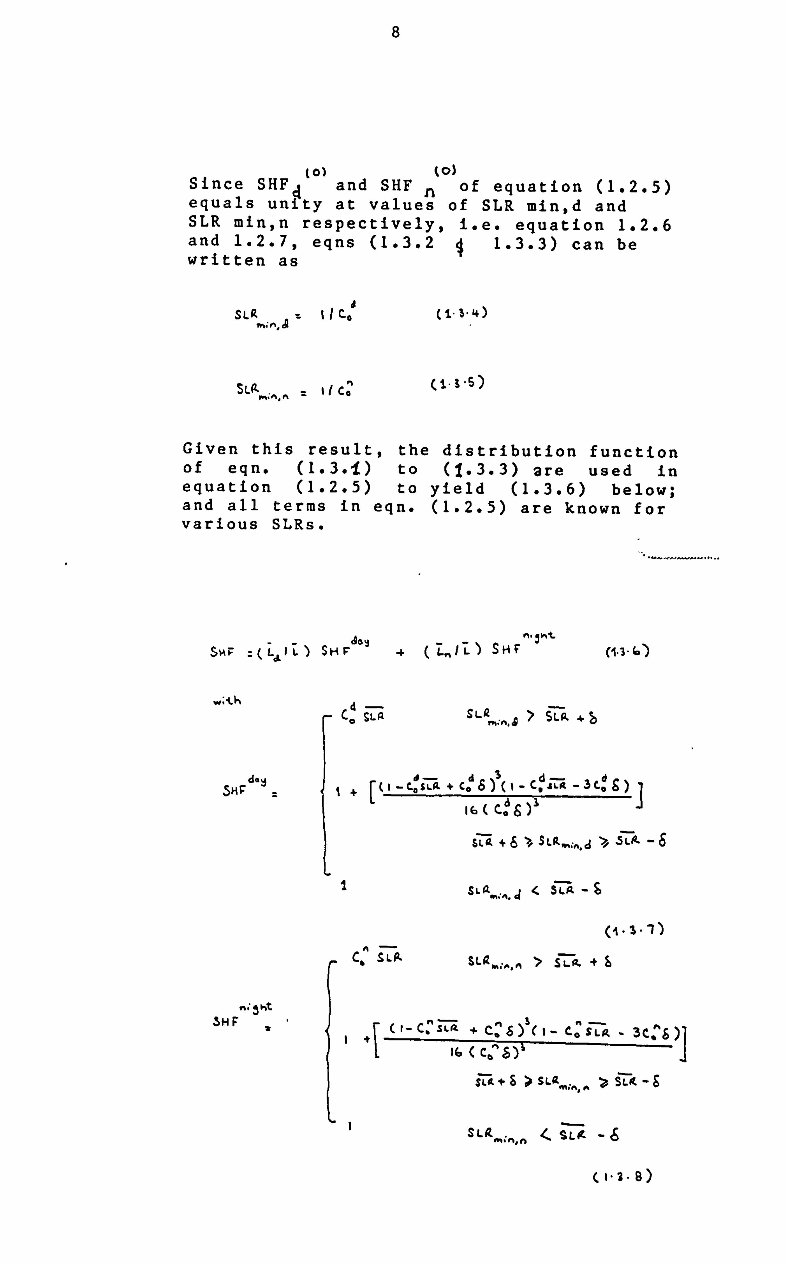
t 0) (0) Since SHFd and SHF n of equation (1.2.5) equals unity at values of SLR min, d and SLR min, n respectively, i. e. equation 1.2.6 and 1.2.7, eqns (1.3.2 1.3.3) can be written as

Z,, ca (1- SLiz -0 3

S LP- M. *, %,, % ýII ca (1-1-6)

Given this result, the distribution function of eqn. (1.3. -L) to (1.3.3) -are used in equation (1.2.5) to yield (1.3.6) below; and all terms in eqn. (1.2.5) are known for various SLRs.

S'A ir :( L4 1 Z) SH P Jag

-4. ( zý 1Z)SH F"' is't

(1.1.6)

4 Co >

d02 d _ C. dr-

Cd ; -LK .6

ý( 1 LK + c. SHP

iL A+&>, sLgý;.. d >, gL A- -6

I

EL +

ht SHF

C. Ra +c + 3C. "6

16 ( co" s )'I-

i-L& +S UZý,. ^,

SUZ .4 ,,, n ý ( 1.2.8)

9

1.4 Application to the Direct Gain House

By definition a direct gain house is one with a large south-facing glazing and thermal storage mass in the interior. It is assumed that the building envelope is sufficiently well insulated and that storage is located so that heat transfer from storage to ambient can be neglected, and that the other thermal mass of the building is negligible relative to the storage mass

The direct gain house is treated as a two mode model, the two modes being the storage S and room air A. As all that is needed to complete the computation of SHF (via equation (1.2.5), are SHF 1 (01 and SHF n

(4)) (namely, the SHF values for periods during which back-up is required), the heat balance equations for the storage are considered. The rate of change of energy in storage at daytime is

Qr d u TS )4 at =

d

The second item of the R. H. S. of eqn. 1.3.9 represents the losses from storage S to room air at temperature, Tc of 18.3*C; (MC) S is the heat content of the storage; Ts is the

10

storage temperature, t denotes t me; subscript d denotes daytime; At denotes length of daytime; (i - F) is fraction of transmitted insolation QT absorbed by storage and does not heat room air; and USPL is the heat transfer coefficient from storage to room air d The solution of eqn. (1.3.9) for is shown in appendix 1 to be

4d -t d /t Ts (t Qýfl

-0 -t 4 /t

U. S, &td e

Wýtrt

Ic - C- c ), / uj"

0-3-10)

(1-3-11)

jor beat* tranSIOr and is the relaxati

' on time. from storage to

room air; and T, (O) is the value of Td at the beginning of the day. Since no solar gain is absorbed in wall during night time, the heat balance equation for the storage at night when back-up is required is

Qvic) cir"Idtn 0uC -T n s35

whose solution for T5n is

Td Tc

where T5a (4t Ct ) is the value of Ts at the beginning of night time, and superscript n denotes night time. We use eqn. (1.3.10) in (1*1'13) to obtain the solution for T 'Ct 0)

F) Q-r (I-e -Alt d/,

us, at

T, ) e -4tý/t I e-

e/ fr-

11

The relevance of the degree days, DDois the fact that it forms a term in the calculation of the solar heating load L0

The energy collected by room air during day time Qj (1) and night time CL

n on a given twenty-four hour day is

cl) At d

Qd + U" ýd (td T. )dtd

0

n at

o+u,, (tn dt ri

0

12

where 'FQT in eqn. 1.3.15 represents the fraction of transmitted radiation absorbed directly into room air during daytime. Using eqn. (1.3.10) and (1.3.14) in eqns (1.3.15) and 1.3.16) respectively, gives

(1) (1-r-) t (I Qd' ý Oy

II-I

&t d

us" Ts CO -r, Ied pr

and LF QT It e:

At' '/t

i e7 6, tn/, r

Qf% -4

ký, ( -rs (*)-T, )T 0- At:

(I- PC &. t"/, c )

See appendices 6 and 7. Both of equations (1.3.17) and (1.3.18) have terms which represent the fraction of Qr which is put to use the same day and the fraction of "residual" energy (which has remained in storage from previous days).

which is also put to use that same day. For a monthly or seasonal calculation, interest is of how the total useful Qr is distributed between daytime and night time over a heating season.

Equations (1.3.17) and (1.3.18) indicate how the residual energy will, on the average, be distributed between daytime and night time. Residual energy QR in storage, is simply that fraction of Qr which is not put to use on that same day, in heating room air; at night time or daytime.

(1-3- 1 q) Qd CD", )

13

(1) (1)

where Qj and Qn are the proportions of QT used in heating room air during daytime and night time respectively using the first terms of equations (1.3.17) and (1.3.18) which are the fractions Of QT used in heating room air in eqn. (1.3.19) yield Qjt, eqn. (1.3.20) below. It should be noted that the second terms of eqn. 1.3.17 and 1.3.18 are the losses from storage to room air at daytime and night time periods respectively.

Hence, Q QT -( GA ( 1) .4-

Qn (1) ) i. e. eqný (1-3.19). Using both eqn. (1.3.17) and (1.3.18) in (1.3.19) yields

' 4t d/,

C a, rfI _D_Atd/,

C It I Qv. Q, -or Atd At d

OK = o, (i-c)t ci-e- At d/'t

)(i-0 -e- &t7/ýz ))

At d

Qk QT (1- 9) Ic f-

&t'/-t (1-e -At ) (1.2, -10)

At

Consequently, the average useful daytime (night time) energy gain Qj (Qr3) for days with no residual energy QH 0 (or days which require backing up) is obtained as (see Appendix 8).

0. (, -F)z (,, -e-

i-e

II

Atdcl-e-

Q=Q,, Qrl Q$L(a) OR Qn = Q, -Qd (1-3-21 )

Equation (1.3.21) provides the solution for SHF (C)j/Qr for days during which back-up is required CL 11 =0) namely

od [ At d /, r )(t e7"'ý'x ) da9

Qý

1

at 4(i- e-(4t4 + A-tn)'% )

11

By Jefination (1-3-22)

d S 14 P C. SLR

do-i

(1-3-23)

lie nee the R HS of e q. n 0-3-22) eVaLs the RIIS of ega (1-3-. 23) OR

14

c(I- P-- &t 4/, t )( I -C

&t'/, c ) Ld

At d(I- e- (&td + &tr, )jt )II

There f are

At

Atd(, _ e-C At's +A: tl)/'c

(I-3-24. )

It can be similarly shown that

p- &t d /Ir

tit 4 cl-e < &tcs. 4_ &t

by writing Q,, 7 QT CLI in eqn. (1 . 3.21) and following the same procedure.

The fact that SHF (0) (days with back-up, QR= 0) is proportional to SLR is a key result. It enables one to perform the integration described in section (1.2), and to obtain a closed form analytic expression' for SHF. With these results, eqns (1.3.22)- (1.3.25) and eqn. (1.3.1) are used in eqn (1.2.5) to yeild the closed-form expressions for SHF as described in eqns (1.3.7)- (1.3.8).

It has been assumed above that insolation can effectively be treated as constant throughout the day. The justification for this is presented below. The only change on considering the effect of using a time- dependent insolation during daytime is the replacement of the constant insolation rate Q, dl&. Ld used in daytime eqn. (1.3.9) by a time-dependent one.

15

The gross feature of the time dependence of the insolation can be represented (12) by a function of the form

i- ( COS'v - COS Q3 )(1.3-26)

whe re angle.

Li 6= Tr &t 67

and

(IJ - 2t

is the sunrise(sunset hour

= 21+

S. 2*7

2 rr /T)

Eill (1-3-R) now becomeS

(rnC) dT Isd/ d-L cl F 9, C cc's W3 US, ( T3 d

s. C

( I-

The soLutiori ol e(ln (1-3-29) Vie[Os

d -týlt r-T, tginw. + s USA

II[I+a,

-r a

sw -c sýn wr _td/t _os ws CTd 0) (- -r,. )e

( i. 3.3o)

16

Repeating the procedure of section 0 4), Q j"I CL n

(1) and Qa are recalculated. ;

he C1

partition of the residual energy QR between daytime and night time is still the same as in section (1.4), yielding the final partition of Q T, between daytime and night- time as

O-F) QTAIý2 F-s"M 033 -A'C CGS WS -i- ( S; r%LJS +SLT COS WS)6' At

d

2 (1 + A"r, Ls 1',, w., -

-%. %) scasw3

- At'l-C

Qd = QT - Q,

These expressions for Qj and Qjare clearly different from the corresponding ones calculated in section 1.4 (see eqn(l. 3.21)). The mair, difference appears at low values of Ic , where eqn (1.3.21) yields

"C 1 4t ci (1-1-32)

()ý :(I-F) Q-r

I sin W. I &, r L (%. &. 3 3) Z(s. r% uis - Wä Co 5 UJ4 )

For commonly used values of, -r, , however, the difference between the two results is negligible. For example, for a &td of 10 hr and a value of IC as small as 5 hr, eqn (1.3.31) yields for Qn a value which is smaller than that obtained by eqn (1.3.21) by 6.4%. With increasing It , agreement is better, and for large values of 't both expressions for Q ri approach the same limit.

3 (i-; )Q,,. t'lr t

17

Also, the limit of Q. for short daytime periods ( &t(i small) is the same for both calculations.

Q'I Ati 3-. LL

I (I- F) Qr ( 1.3-35)

1.5 Application to the Water Wall House

The house to be considered has a glazed, south-facing water storage wcIll. The absorbing surface of the water wall is taken to be equal to the glazing area. The houses's other thermal mass is assumed to be negligible relative to the water wall. The use of night insulation is optional and will be treated in detail below.

The wall house is treated with a two-mode model, the two nodes being the water storage S and warm air A. During daytime when back- up is required, the heat transfer rate from storage to room air is represented by

dd, d) -U (-r

= (OLQ, /&t J$k 'Sd -d) -d-TS / dt

- L(5

A( TS d-T,

where o( is the fraction of transmitted insolation QT which is absorbed by storage; Usaj is the daytime heat transfer coeffi- ent from storage to ambient; and U $A is the heat transfer coefficient from storage to room air.

One further approximation to be made here is that the relative fast rate of heat transfer which results from natural convection within the water wall allows the treatment of the water wall as an element of negligible thermal resistance. The convec- tive heat transfer coefficient within a water wall can in fact be calculated from the theory of natural convection of a fluid between two parallel plates (13).

18

For the temperature differences typically encountered in such systems, the thermal resistance to heat flow by the water wall is of the order of 0- 5% of the thermal resistance to heat flow from the inner surface of the water wall to room air and will hence be treated as a negligible contribution to the overall thermal resistance to heat flow from storage to room air, I S'k

The solution of eqn (1.5.1) for Tt is shown in appendix 2 to be

d tQ, (, - (it ddd

td/ -C d -rs W)

- Tý =u so. ( Tr. - 1-. )(I- Eý dCU

t Ud US. +ud 4Lt

SA

where -C -I, (o) - -r, ) e7 (I. S. 2)

USA * Us )

a

and is the relaxation time for daytime heat transfer from storage to both room air and ambient; and T, (o) is the value of T3d at the beginning of the day. At night time when no energy is absorbed by storage, the heat balance equation when back-up is required is

An (M C)s d TS 0 USA S CL

� '. 5. ")

whose solution for Th is 5

n -tn/, Cn TntA Tc.

Uso ( Tc - T,, '

n U. SA +u So

75, d

( Atd )_ _r. ) e-tn Itn

(1-5-S)

19

where TSd( At a)

is the value of T. at the beginning of nightime, superscript rx

denotes night time; and Am

T= (fn C)s +u50.

A distinction is made between the daytime

, and night time heat transfer coefficients f rom storage to ambient ( U$&J and Usa ' in order to allow for the effect of night insulationpshould it be employed. Using eqn (1.5.2) in (1.5.5) yields the solution for T, '. '(tn ),

T. "(tn) oLr-, ( i- e -At d /, td - tn

e dd 4t C USA + U511 )

dd_, dt4/ Xd _tm/, C n uso ( Tc. - To e

u5A +d

I

SCL

rl e' tll/-cr, Uso- ( T. - T(L

USA + USc),

+T Tr At

dd)et n/. en (1-5-1) 3

The energy collected by room air during daytime (Qj (11 ) and night time n

(1) ) on a given twenty-four hour day is

d

U (Tci( Qd td) -

T') dtd I

SA s C. 0

n

us,, ( Ts" T, )dt co

20

Similarly, the energy lost from storage (11 to ambient during daytime EA and night

time (Enýil) for the same twenty-four hour day is

-d(td) d)

dt: d

I- Týl

At r%

En = TSM (tn)- 'r. r' )d t" ( 1. F. II) I

$*- s

a

Using eqn (1.5.2) and (J. 5-7) in eqns (1.5.8)-(1.5.11), gives

11) d -At d /, Cd

cz - Cý ,u SA t (, -e 3 06" n

USA d

+u SA

'ý d( TS (0)-T, )(, - e-

dLt ci/ -c

ö)

res*. ducLL

- L, waLL Load

(I-S. 12. )

(0 r% &t d/, rd 4t n pt Qn ) (I - e, - dda. &t ( USA

AL

+u 'Slk

.n( 'r. (o) - T, ) e- I *c

(ie- At n/, r n

resýd tA(3

- waLL

0.5-13)

21

(i) ci d- 4tý/ td *1

Id =dQ, -is, 1- ud

go-n

Id d +UT(T to) T )(I- e C.

resi', d u a. L

+L waLL Loa4

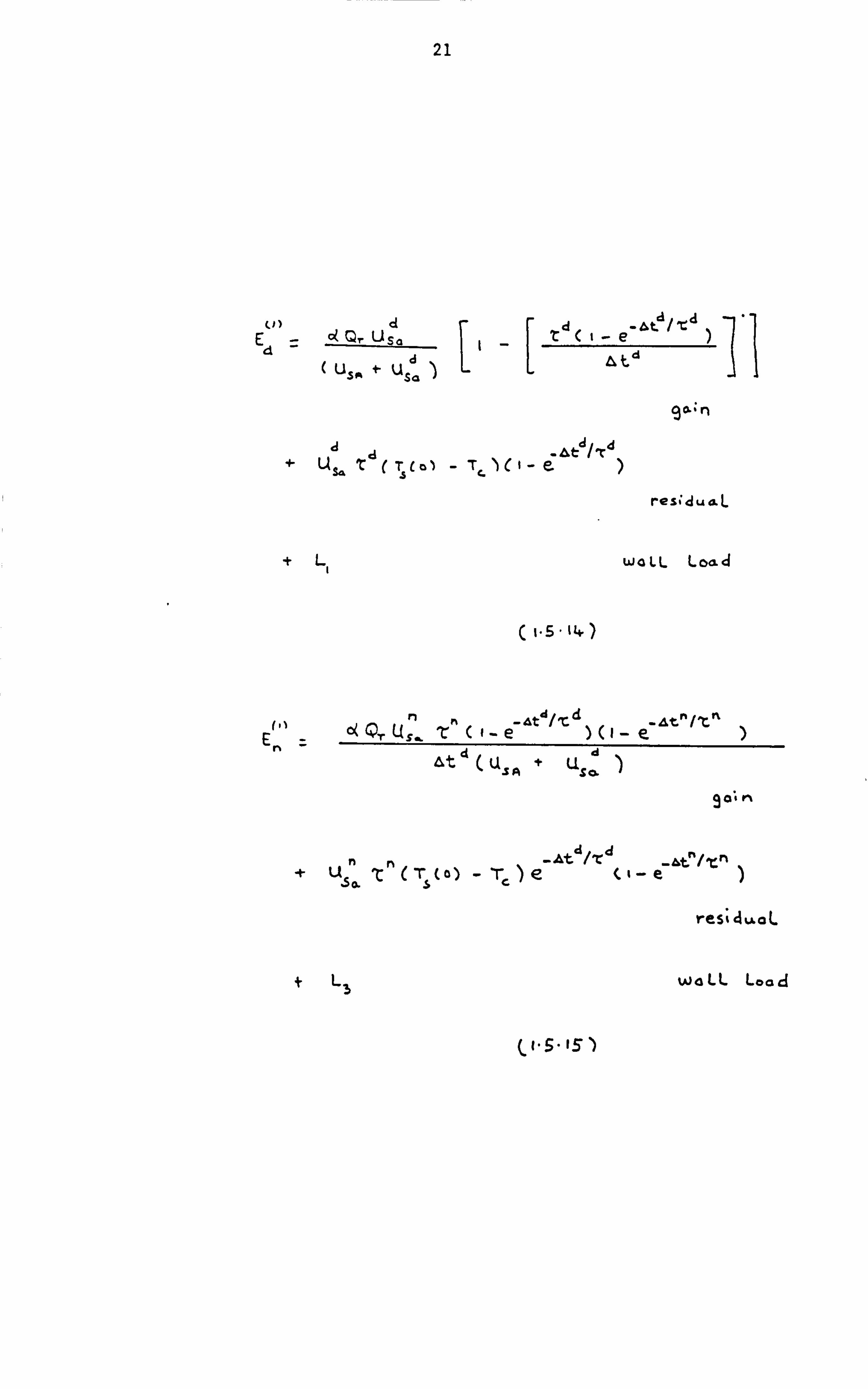
I-s - 14. )

(, 1 :ZQ, U, _C� (f_j�, d ,, dn/

't

EM =- S- d) ci ( e-4t

4t (U u S(DI-

9 0,6 r%

At d

Ir d &t7/, tn

+ uýS 't (T (0) - r, )E(i- e7 s

+

resi 4%.

AoL

WaLL Load

22

Eqn. (1.5.12)-(1.5.15) each have three types of terms. Terms proportional to cLO, represent the fraction of the absorbed solar gain, ULCLT which is transferred either to room air Qa(" $ Qn (i) ) or to ambient (E8(1)) and (E (11) on the same day. Terms proportional to A Ts(o)- T4 represent

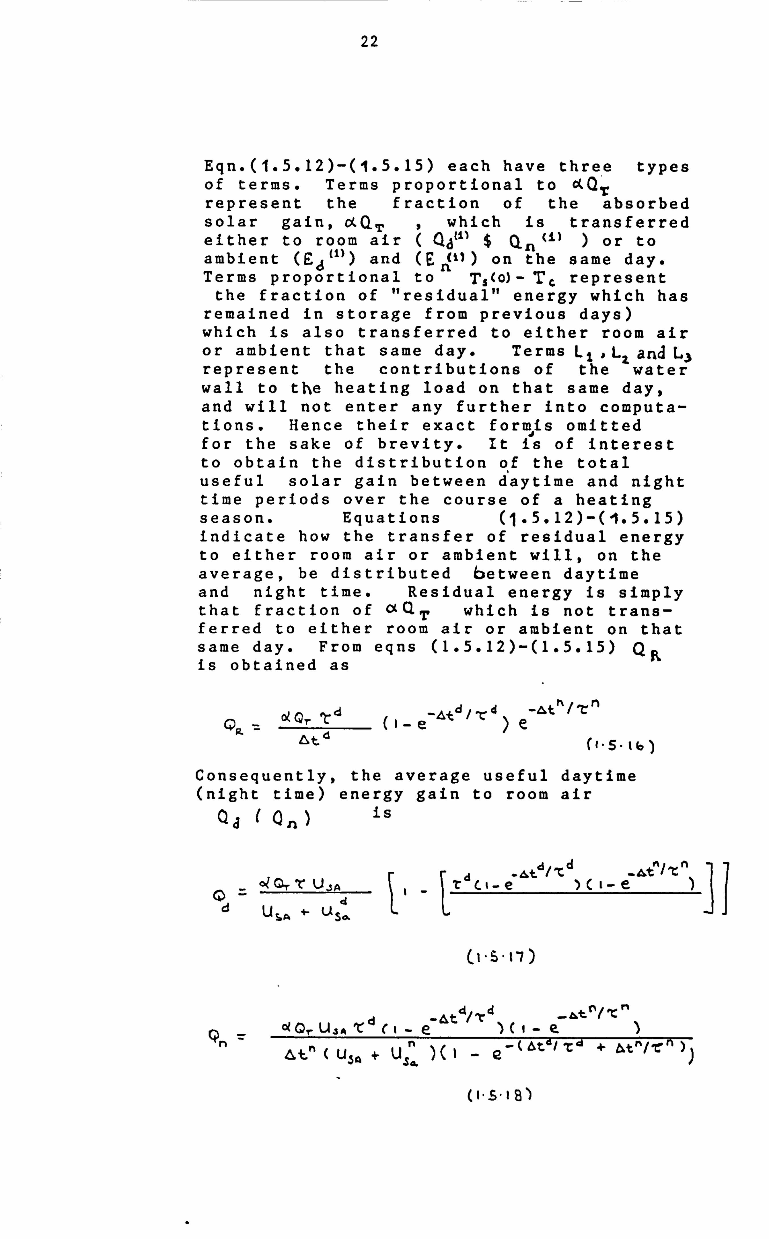
the fraction of "residual" energy which has remained in storage from previous days) which is also transferred to either room air or ambient that same day. Terms L, , L. and L3, represent the contributions of the water wall to the heating load on that same day, and will not enter any further into computations. Hence their exact fornLis omitted for the sake of brevity. It is of interest to obtain the distribution o, f the total useful solar gain between daytime and night time periods over the course of a heating season. Equations (1.5.12)-(-1.5.15) indicate how the transfer of residual energy to either room air or ambient will, on the average, be distributed between daytime and night time. Residual energy is simply that fraction of ot QT which is not transferred to either room air or ambient on that same day. From eqns (1.5.12)-(1.5.15) is obtained as

±01 Td (i- e-&+. d /, t:, d)

e-At ft /'r

Ltd (I. S.

Consequently, the average useful daytime (night time) energy gain to room air

Qj ( on ) is

41 -, &t d Pt d-4; 0 It n

C)l UJA Ic

ul u So. L

(1 -5- 11 )

d

(Atd/ -cd

8')

23

Eqns (1.5.17) and (1.5.18)

solution for the SHF for days back-up is required, namely

5HF d Ld =(L

and Q

provide the during which

QIE)=c SLR 0 (I. S. 19)

(0) SHF

P) C), I En

-= ([Iýn) Q, I Cal 5LR

where rd USA 4tdprd )(1-e - 4t7/IC

0 =( L/ Ld d USA +U So. (t-e-

nL 0( USA 'r d0dI e- &tr'jCn

CO -d 'ý' Un 4ýjc (USA0, e -. C d+&, Lr% /. C n

The key result is the fact that SHF""is

, proportional to SLR and the closed-form expressions for SHF are eqns (1.3.6) - (1.3.8).

1.6 Application to the house with Massive Storage or Trombe Wall

The house to be considered here has a glazed, south-facing massive storage wall (MSW). The absorbing surface area of the MSW is tcxken to be equal to the glazing area. The house's other thermal mass is assumed to be negligible relative to the MSW. The use of night insulation is

n optional and affects the value ofl-I SI_ t The night time heat transfer coeffic ent from storage to am bient. Treatment is made of the two cases of vented and unvented MSWs.

The heat balance equation for the storage is considered with the storage represented by a single temperature T. . The validity of treating the non-linear problem of heat diffusion through the MSW by a linear one -node model, for the calculation of long term thermal performance for wall thickness of practical interest, is established in (14). See Appendix 3.

24

Based on the assumption that the non-linear solution for MSW temperature TS does not introduce much difference to the one-bode model (14), during the daytime when back-up is required, the heat balance equation for storage is

41 C rn c- d T'ý td +-d tt" Usa, T"

(T" -T, )

V4 5

where (MC), is the heat content of the storage; superscript d denotes daytime, Ta4 is the average daytime ambient temperature; t denotes time; At d is the length of day time; c( is the fraction of transmitted insolation QT which is absorbed by storage; U dis the daytime heat transfer coefficient aa from storage to ambient; and U,, is the daytime heat transfer coefficient from storage to room air, given by

usw

u5 + U5W

�er%t

urlyente d MSW

( (. 6-2)

vlente4 MSW

In equation 1.6.2, U,,,, is the heat transfer coefficient from storage to room air, through the internal storage surface, and U

,.,, t is an effective heat transfer coefficient which approximately represents the effect of venting.

A fairly accurate accounting for venting on long time scales (a month or longer) by introducing one effective value Of Uvent has been demonstrated by computer simula- tions of vented MSWs (15). The justification for the treatment of insolation as a constant has been presented in section 1.4. For the one-noaa model, U

Sw is given

by

Sw ( 1- 6-3)

25

where U., is the surface-to-air heat transfer coefficient, L is the wall thickness, and 1ý is the thermal conductivity of the MSW material.

The solution of eqn. (1.6.1) for Ts (t is t dprd Ad td/. Cd C Te )(I_e T

ýOIQT O-e [us

. T., L

&t d( Ud t- Ud)I( Ud + USd W So Wa

(S. E. L4. ) 4 (; co _T)e

where

't d= (m C), I(u, vi Sa

and is the relaxation time for daytime heat transfer from storage to both room air and ambient ; andT (0) is the value of T at the beginning of tte day.

The heat balance equation for the storage at night when back-up is required is

(. C), CIT'rI dtn =0- U" ( 7ý - 'r r' )- USW (T n-T) S*. 0. S b. f. )

whose solution for TSnis

unSCT, T,,. m )ci- e- a ri (us, + U5ý

PC ri

26

where TS d(

At j) is the value of TS at the

beginning of night time; superscript n denotes night time; and

'r tI% = (rn C), I( U. " +- USCL )

The distinction between U and Un sa. is to allow for the effect of night insulation should it be employed. Using eqn (1.6.4) in (1.6.7) gives the solution for Tsn( tn)

TS rl (tM) - TC. J. ( CD, (I e--'t

a/, Cd ) e7

t n/,, n

n us, c T, c e-'n

USW US ') d/,, d -tn/, n

USaL (Tý - T. ' )_0 - e-At e dd Uj +U 54L

)

+( Tý d/,

C d

e7 tI/ -C n

< j. 6. q The energy collected by storage on a given 24 hour day is composed of three components: (a) heat lost to ambient; (b) heat transferred to room air; and (c) "residual" heat which remains in storage and is consumed on subsequent days. Following the procedure detailed in section (1.4), the SHF for days during which backup is required is obtained as

SHP Cd. SL IZ d0

SHF(ol, Cn. n0 SLP

where

Ud+ ýLtr, b4 50

(I. (a. 12)

us T6CI_ e7. atýl, _t dl (I_ ,_ &tri/, C m)

LAS, +Und e- (&td/. rd + &tn/. tn

Sol

(1-6-13 )

27

The final expression for SHF is

SI, IF = SHF Lj IL+ 6-14.

where SHp Jay

and SHFf'19*nt are the average daytime and night time SHFs respectively. if the parabolic distribution function described in section 2 is now employed, a closed analytic expression for SHF is obtained, with

d C, 'X A

(%-C! -jC'% +C C'i %A -3 + 06)(1 _6) 16)3 16 C CO =. + &'> '# XA-6

< X-M -6,

SLR n. -M, a

( "'5'

n SL 1Z CO h-E

V4 3'6)

SI Ca' + C. " S)(I-C %A C,

16 ( C, 11 6)3 'k 3CA - (S

n

116

where X. average SLR value.

1.7 Application to the Direct Gain House with An Attached Conservatory

In keeping with the original work of Gordon and Zarmi, we consider the relative proportions of the size of the conservatory to the direct gain system, where B is the quantitative heat transfer proportion of air from the direct gain system to the conservatory. Then a study can be made of the effect of factors as the size of the

28

conservatory on the direct gain system. It is further assumed that the complete outward wall surface area (south facing) between the direct gain system and the conservatory constitutes the system storage mass. The direct gain system is considered at temperature Te . As pointed out in section (1.4) the effect of considering a constant insolation rate QT on the computations can be assumed negligible. The storage is considered at temperature T, a during daytime, and T. r' at night time. Tro is the average unifo Im temperature of the conservatory, and Ta the average daytime ambient temperature. A consideration of SHF on SLR for such a system and the influence on it of the building and climatic factors will be made. Evaluations of the performance of such a system as opposed to the direct gain house considered by Gordon

and Zarmi (1) will be presented in

section (2) below.

heat The daytime., balance equation for this system considering a3 node model is

Crnc)s dTs cl 1 dt d: (1-6) 1 «, -F) Q-rl ht d)- US; %

(T5d --Tý, )1

d u ýT

ca's eo

storage superscript d denotes day time; is the length of daytime; F is the fraction of transmitted insolation QT which is not absorbed by storage and hence directly heats room air; Fe. the fraction of transmitted insolation ; through conservatory not absorbed by storage'(wall storage in conservatory ), and directly heats the air in the conservatory. U SA and UcO, 5 represent the heat transfer coefficients from storage to room air and conservatory to storage respectively,

where ( MC ), is the heat content of the

29

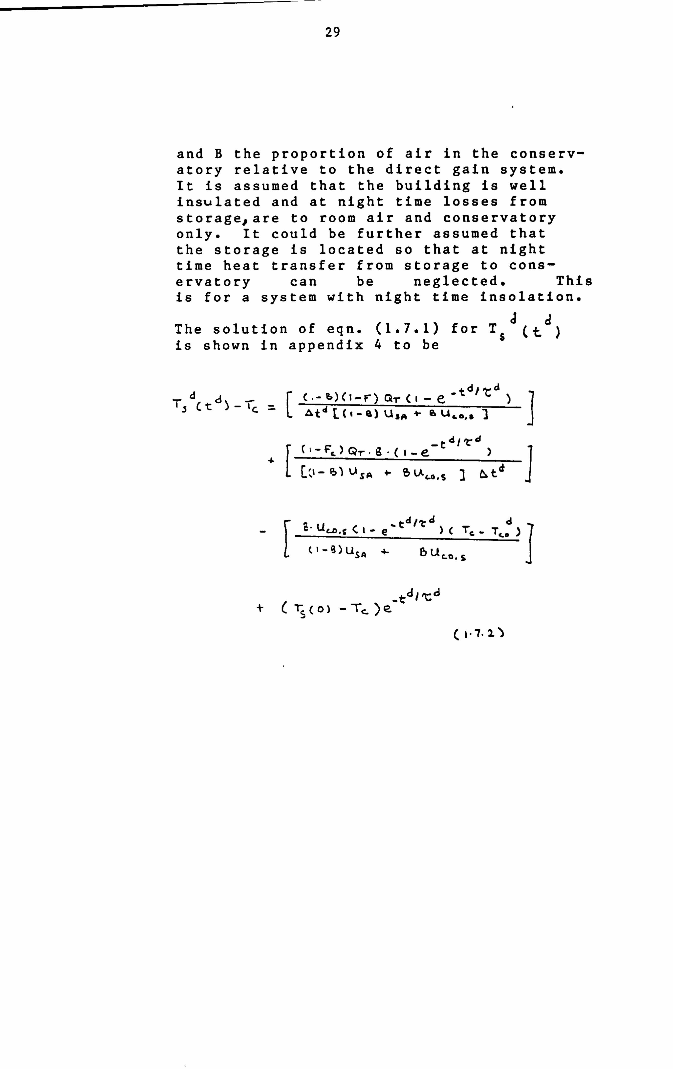
and B the proportion of air in the conservatory relative to the direct gain system. It is assumed that the building is well insulated and at night time losses from storage., are to room air and conservatory only. It could be further assumed that the storage is located so that at night time heat transfer from storage to conservatory can be neglected. This is for a system with night time insolation.

The solution of eqn. (1.7.1) for T is shown in appendix 4 to be

43 C (I e- - tdt td) ICt)-,,, =I At" L0- 6) UsA 4- 1& u..,, II

-td iv '

[�, - pi) u SA 4» 5(-Ä". s 1 Lt

1

td pt 4CT, _ T,,

d e

tl-B)USA 4.15 Ll

rs ( 0) - -r, -

) e-t dI ,-8

( 1.7-1)

30

or

Ts d Q-r (k- e-

td/ rtd )(I-F sr -sF,

)-

tUSA+ La, 0]I

t: cl I't cl

lb) U-5A 1- 5 ULO. S

aý-T, )e at'r, d

where

0) LASA + 13 LAf_0,5

and is the relaxation time for both heat transfer from storage to room air, and conservatory to storage; T, (o)is the value of TSa at the beginning of the day.

The heat balance equation for the storage at night when back-up is required is

("C)s 8Tsml dEn0-0- 5) [ USA (Tn S

This is the equation balancing heat transfer in the storage assuming night time insolation is employed. the first term of eqn (1.7.1) is zero. So are the third and fourth terms respectively. Equation 1.7.1

reduces to the original form due to Gordon

and Zarmi (1). If however no night insolation is employed, there will be losses from

storage to conservatory and the first and last terms of eqn (1.7.1) vanish. The third term, however, now becomes

31

Term 36[ USILO C -r sT C4 n

or Term 3 16 C -r" - -ra (-I. -? ) . ") I i. e. assuming the situation in týe cons'ervatory represents night time, outdoor ambient conditions with allowable accuracy.

Hence, the night time heat balance equation can be written (for the case of no night time insulation) as

)S . n, +, I (TYI C n_ TS

-a ý U, -.. 5. c -r, " - -r.: )I (I. I. !a) We note that when (B - 0), the equation 1.7.8 reduces to the direct gain system without conservatory i. e. eqn. 1.3.12., the solution of eqn (1.7.5) can be shown to be (for the case of night time insolation)

7. T, C --r, )e IC n

where

11 (% = (MC), I CI-e') USAC 1-'7- ia)

and is the relaxation time for heat transfer from storage to room air at night time; where TSJ (at d) is the value of TS at the beginning of night time, and superscript n denotes night time.

Using eqn (1.7.3) in (1.7.9) gives the solution for Tn(tnjas

S

PC

TS n (t &t4((1-6)U. SA + &LIL"S)

-4t al xd di

-ý pi - u. -0-$ (t- p- )e -r� - «n. -b )

(-t-, býUSA t- Eý LLC_C>. s

1

- &0 / -C "

_tn,, -

Ts P- e

32

0

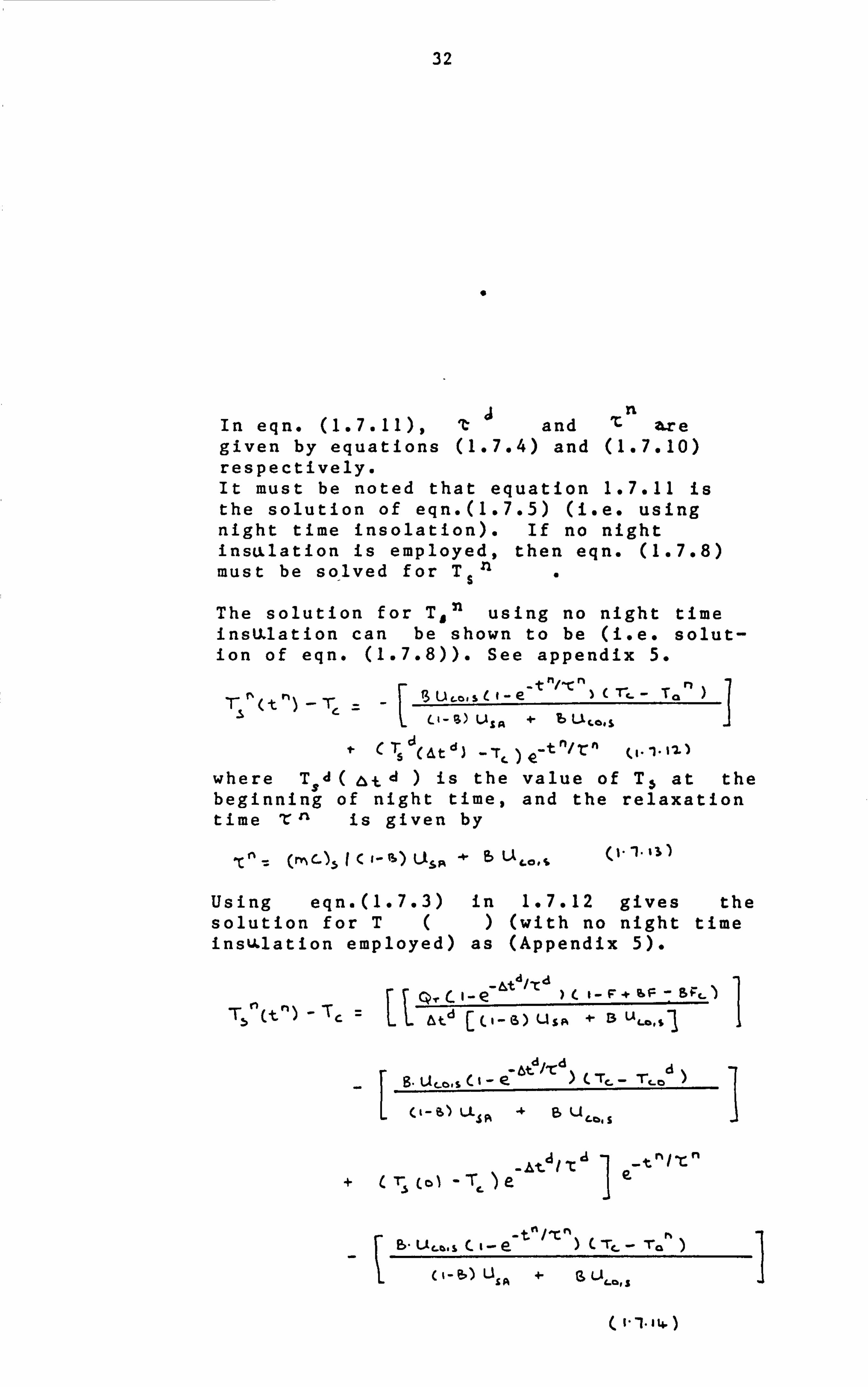
In eqn. (1.7.11), Tj and T- 46r e given by equations (1.7.4) and (1.7.10)

respectively. It must be noted that equation 1.7.11 is the solution of eqn. (1.7.5) (i. e. using night time insolation). If no night insulation is employed, then eqn. (1.7.8)

must be so-lved for TS11

The solution for T, n using no night time insUlation can be shown to be (i. e. solution of eqn. (1.7.8)). See appendix 5.

T_ r) -TetT,, n

Li- U" 16 U'O. S C T, 6(

4t d3- -r, ) e- tn/, n (I.

where Tsd &+ d) is the value of Ts at the beginning of night time, and the relaxation time T"' is given by

Ic- =I( I-rs) Lis" - e, U,. ",

0.1.131)

Using eqn. (1.7.3) in 1.7.12 gives the solution for T) (with no night time insu. lation employed) as (Appendix 5).

Q, C I-e- &t

d)C

I- F+ SF - SF, )

At d C(I-S)USA BULO'. ,

, -C" I

btý/'cd )c -rc - Tc d)

B. uc-o. s ci- e7 _Z, 1 ct-ßý UL4f% +a

dLcb. S1

-t Te.

B. LA Lb. sCI- e- t)C

-rL - T, )

(ý-N) Lie-als

( I. -T. I ti. )

33

where tcl and T-n are given by eqns. (1.7.4) and (1.7.13) respectively.

Thus equation (1.7.11) and (1.7.14) presents us with the solution for T,. n (trý) with and without night time inskilation respectively. In equation 1.7.11 the relaxation times ( Td . r- n) are given by equations 1.7.4 and 1.7.10 respectivelyeFor the use of eqn. 1.7.14, It C1 # rt rl are given by eqns (1.7.4) and (1.7.13) respectively.

We should now evaluate the energy (for a given twenty-four hour day) collected by ro.., ai r during dayt ime (QjM) and night time (Q The later will be done for both the cases of night time and no night time insulation.

At d

F Q, -T, ) dtd

n At

U., (Tr, ctm) - T, -

where FQ T itýeqn. (1.7.15) represents the fraction of transmitted radiation absorbed directly into room air during daytime.

34

Using equation (1.7.3) in (1.7.15) gives (see Appendix 9).

USA Ci-F +- eF* -6;: C. ) T.

aCI-e)-A

FI( 1- 5) USA +B Lk,,,, 11

1

&t

UsA T, (o) - T. ) 't dc t-e-

at d /, td )-

where Lj is given in Appendix 9.

Equation (1.7.17) has three types of terms. The term proportional to FQr represents the fraction of the absorbed solar gain, FQr which is transferred to room air. The term proportional to T. (o) -T r- , represents the fraction of "residual" energy (which has remained in storage from previous days) which is also transferred to room air. The term L, represents the losses from room air to conservatory. The exact solution will be presented by eliminating the second and third terms of eqn (1.7.17)t<1.7.18).

Similarly, for the case where night insulation is employed, using eqn (1.7.1) in (1.7.16) yields the solution of QA (has (see Appendix 10).

(m; 7QTUSP"C, (, I-e - &t Id I't d)(1-

e7 E (I - 6) U,, i- Bu Co's

I

4- U. Sp.

T- e_

- L2

where rn = rl IF

m- At

a PC 4 -&t

F% I t" i Ll u P, - U,.,, -C (I-ee (T. -Tc.

C %- 9) USA 48 ULO, 3

4 1.1. IR)

35

In equation 1.7.18, T9aT, are given by equations (1.7.4) and (1.7.10) respectively, and ý=I-FP

In order to evaluate the energy collected by room air during night time for the direct gain system with attached conservatory and no night insulation employed; the solution for the heat balance equation, (eqn 1 7.14), is substituted in equation (1.7.16): ýJ,,

rn are now given by equations (1.7.4) and (1.7.13).

Hence, (see Appendix 11); distinguishing the energy collected by room air at night time for the direct gain system with attached conservatory, and no night time insulation as Appendix 11 gives

L t-'1.2o) b d Qd

n/ Cn where USA S-U, C"S T" At- 4- -I) Cr. - T'.

((, -B)ULA +- 5ULO's )

As noted in Appendix employing night time the energy collected equal to L,

(I. 1.11 )

ll, the effect of not insulation is to reduce by room air by a value

Residual energy is simply that fraction of FQT which is not transferred to either room air or conservatory on the same day. It is evaluated using the terms in FQ T in equations (1.7.17) and (1.7.18) for the system with night time insulation as

36

QT

d e'

at d /, Cd For + SA

--- dI (1-6) U-C A+

au LO. SI& t7

QT U5A 'tr( 1- f- )(i-e

&td((%-iS)Usa * "Ca's )

d -At dI

It d

46tdltd -at'jrn Or 0 SA

I 't ci-e)- ItNt - 't (I-e Kf-e

atd (( 1-0 U. S, + V,,, S )

olk

At &tdttd

(,

rnp-Or USA [,. r" (I- eý T-'ci-e )O-ei -6)usok+ Bu,., s Atcl

( %-1-22)

37

The average useful daytime (night time) energy gain QJ(Q n) is evaluated by solving eqn. (1.7.17) and (1.7.18) simul- taneously. Eliminating the terms in TS (0) -Tc and L IýL 2) yields (see Appendix 12) for the system with night insulation.

SUMMARY

From Appendix 12 to 14 we summarize as follows.

For a direct gain system with an attached conservatory, the useful energy gains Qd((),, ) at daytime and night time are given by

(A) System with night insulation (A12)

The average useful daytime (night time) energy gain Qj Qn ) is

Qd m Q, , 1- 9) "CM f- 4t d pt de

-atm/tn ne -&td /, td

d Atdltd usak (I -e- )-

a tý ix at d ýo c (1- a) uo + r'e-4 +Itacl-e

T" e-' at d /, rd

1 12- -at"/, Cn ) 4- L2tCi-

e-&t d/, cd

&td prd ( e- 44 mp, m)+ _Cd _ e-,

&+dtrd

"3 1 ma d oý

( "1.2)

38

-, &tci/Zd - at , /-c (I-e at-, ' /tn &td/td e- ) +- rd ct-p-

rn"' F Us Aac e- &t

At d e, 6ta Icd

&t d 6) U,, +- E, U,,,, M e- Ae I'Cdci

e- Ct. /, Cm +I d(, _e-, l'6l

Li'tme-, &td'Xd (I -e- Atr, I -t 11

) I. Lz rde-, ttd I 't d

'tr'e- 4 t'd pr dci

e-- &tnl 'Crl ), rdC, - &tl Ird

:[/ m2 o! j

(1-1- 14- )

and from SHF d (a)

= co (I

SLR we obtain

cc 61CI: d

(I-F) T-,, e- &td/r dc &tflitm )

Cnp-At-ITOC at 4- XCI-

- ry%* F UsA Z"' ( i- e- &tl/zn

)cIdCI- e- dt4/ 7: d)- &t4l e-4t'j/-t-d

-a)u )Ltnr-, &tct/, Cd(l_e-&trl/. Cn ) e

L. Zna -&t ditd

o -e _., tn/tei

)+ Lz TdCI- 4E- bt d/ td ) d /, rd - dt" /-C d e_&td/Td (. te

rl C I-e n e-6t.

11-rd 6tnjtn ) -C d e- btdl-td

F LA

ätd (( -la) Lis A +. a LAc... s 3E zr%, --6týlta Ci- e-At"lzr'3

Lt tm e- ät

dit d(t p--,

N tn lr, 1 )+ 'Z: " (1 p- - ätli 1 Zd

t(Ne At ej pr

wý*re C u.. 16)

Qr E3 "1']

cu 4-

Tn USA

(rAC). $ = 'tke--aL -ass 4 storage ( q. 2AIo S' 3- Im 1 14 )

39

cAd re I -((I - S)F

=-F *- 9; - I!, r-c-

'd/ 'r daIT, Ci 'A 3f. 00 &t USA - Ur-as -T,

(I-S)US, q +

-&t dizJ

e- At"k Tc. _T,

d

L2 B. ua-U Los e_-,, )x3 600

( I- USA +5U. S U3A 1'7, U, o. s (. WIM'K 7.2 q )C

USA U, G,. S L: rjr"IKh, j

= ý, JJM'414]x 3600.

T. and Tcodare the room and conservatory temperatures during the day respectively. TqO dis given by eqns 2.43., ie.

Tf d F: P, Uo-q, 16ý, Clr + ct- a) ; 0,3 /ue$ a FR Ue, $ + r" Irj-'L CP

I+ To

4 1-7.. 30)0

Tc- ý 113*3 ", -' -2q-3 *K

The equivalent heat transfer coefficient is from eqn. (2.2)

U8C I- B) U sak LICOS (1-5) USA + buLos.

U S, ý andLl,. s are the heat transfer coeffi- ents from storage to room air and conservatory to storage. The heat removal factor for the building envelop treated as a collector is from eqn. 2.11.

cp FK rn; r%4-L Uel,

in eqns 1.2.30-32.

40

ý in; i. L. is in ( 'V9 m 12 s Xcross section

Of flow). U eq in (W rn 2K). QT the transmitted insolation in (W/ rn2-/ day). C the specific heat capacity for air at constant pressure, taken as 1012 (J/149k) B the ratio representing the size of conservatory compared with the building. Size (cons-) + size (B-) = 1. To-the amb i ent temperature (Ta - 11.6 (284.6 * K). &+ in eqns. 1.7.23 - 1.7.29 is taken as a day length of 10 hours (in hours). F and Fcthe fraction of transmitted insulation into room and conservatory not absorbed by storage, e. g. F=0.2, FC = 0.5 (F << If the windows and doors in house are assumed closed, then air moves in by infiltration. Hence the use of rAl, f

. rIL in eqns.

1.7.29 a-d. When open, *wind and stack forces come to place, and r; niný., L is superseded. In that case invent- is used. Derivations for r; iimýiL qnd" Vent of flow (see eqns. (2.35) and (2.66); lead to

0.2e v-0.5 HI. -, P. ",

. Ir potm 2 7ý,

T. T,

II -R.

T., C.

o2 C*(Il. 2ý L-L ý'Lin

ITO 0.53 H(

TA Tc.

U31S

and

41

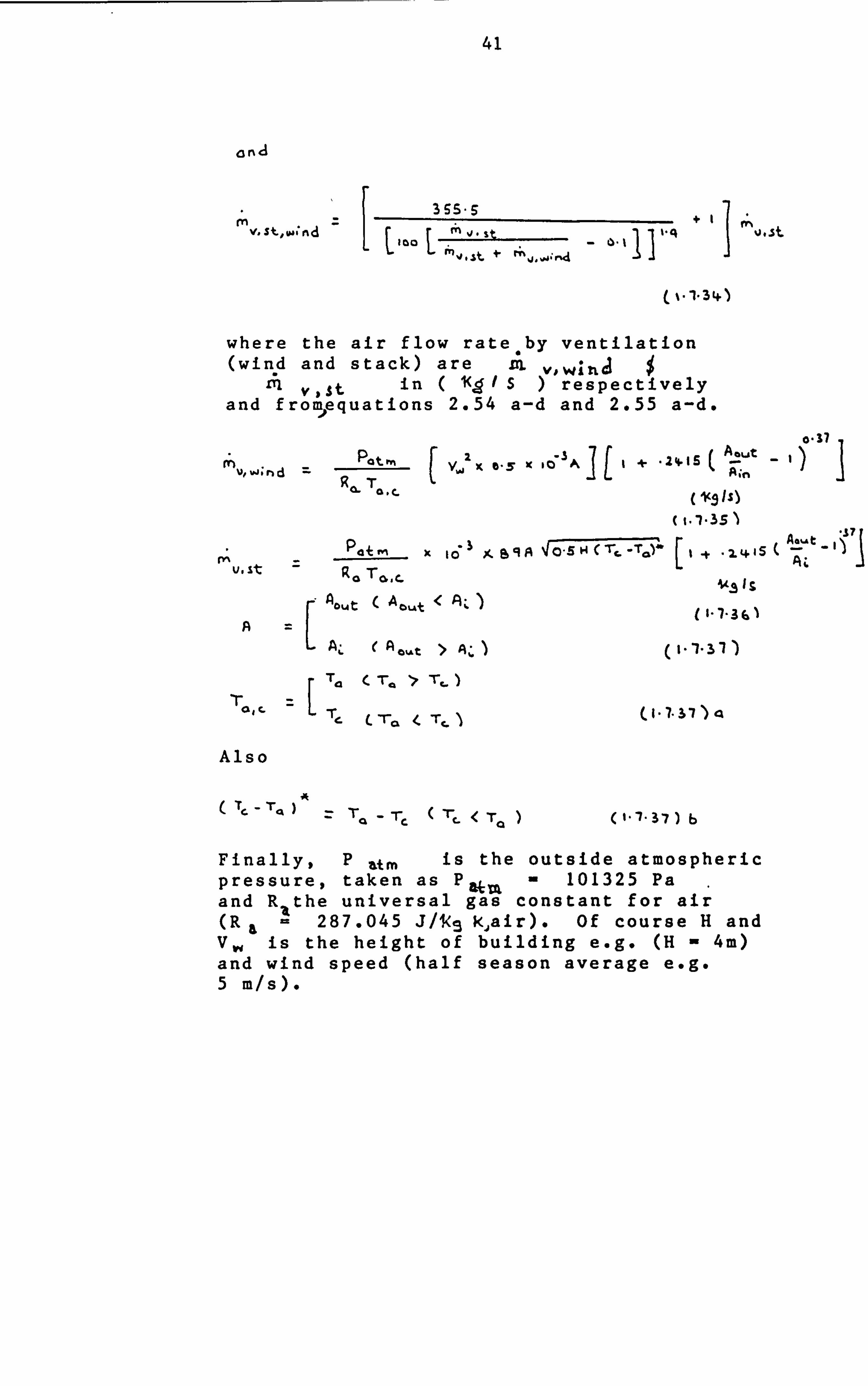
anA

rn + V. st,.. *Md r; l V'st

(%-3 L* )

where the air flow rate. by ventilation (win. d and stack) are 11, V, WirLA

$ ri V'St in ( 1(, g IS) respectively

and fromequations 2.54 a-d and 2.55 a-d.

17 P. t

A.,, t

To. X 8-5 +(A;

n 4L

Pat mxqA 40-S HCr, -T. )-

V. St RCI TOI. C. A.. t ( A.. t < Aý

Aý A , ýt > Aý

T4 T, > Tc.

-r. e. T, -

Also

T, - T, TQ _ Te (T - C- < To 1"7' 37

Finally, P atm is the outside atmospheric pressure, taken as Pk. = 101325 Pa

. and RA the universal gas constant for air (R a 287.045 J/VS k, air). Of course H and VW is the height of building e. g. (H - 4m) and wind speed (half season average e. g. 5 m/s).

42

(B) The case of the NO night insulation (A14)

The average energy gain the case wi replaced by is true for and C,

I-A-

useful daytime (night time) Qa* (Q

" *) are identical to

th night'linsulation with L2 (LZ 4, L3 The same the coefficients Ca'*

. See discussion (A. 12).

L2 = L; L + L3 c

ci c f%

%, Q r% , CO 0(sa mp- )

where L, is given from (All) as

-, ät'/ Z'- A't m /, cm ) K*(Tr -, r d

L3 -- 15 - us ZU to s-�, r% cý-e -0 )

(1-b) U$A +6 uLo,

s

( i. 1.37) od

where

I-VU Usrt

c r,

43

A(13) presents, K* values lie in the range 4ý*

2.0

The fraction K* is fully described below (see A. M.

5.0

Colaer days and warmer days nights in conservatory and nights

in conservatory

44

The typical K* value for our "reference" house with reference conditions (A13) for a given T co is

-r, ., =I E4.0c -rc. = 18- 30C( ib 5 *F )

V, V, -= -o-6((; ep;. *, g .A( 13 ))

K* is a climatic factor.

We note that for the case where night insulation is employed we may assume since no heat proceeds from room to conservatory (Tc - T, O""') = 0, and Tlj It" but are given by 1 7.27 and 1.7.28.

Hence f rom eqTi 1.7.37j, K* =0 and the expressions for C0 'd* 9C0

n* become identical to the case with night insulation, i. e. L: k = 0. Therefore a value of K* = 0, represents the case with night insulation )If Zc' -4- 't 11 )., e(Ins- no LrxsuL8Ucn become identical to those for night insulation, f (L Z ), whereCJO are now given by eqn 1.7.27,28.

j n. JA TI* With these compute

,d values for Co,, CopC, PCO from equations 1.7.25 - 37g, the use

of eqn 1.3.7/8 and then 1.3.6 yield the values for SHF as a function of all the parameters appearing in eqns 1.7.25 - 37g, where in eqns 1.3.7/8

d LP, -=t1

Co rnq r', a

an CA

-SLP -3 q

45

and also dad

IL) St-IF THP SHP =( Li IL 40

1.8 The Effect on Qd, Qn AndSHF oý the Daytime losses Lifrom room air at T. to conservatory. f(TC -T, d

.0 (Case with conservatory and Night Insulation. )

In this section we develop express-j ions for Q d(L) 9 Qn11)* Qd4lQn, and C, Carl *, in terms of the losses from room air to conservatory at daytime, L1. This permits us to study how these losses will affect the coefficients C. 8

and C0n; hence SHF.

We also justify the solution for C. and Can in our case, by assuming that the conservatory is re moved (B - 0), hence the losses (L jý JO 'L2- 0) equal zero. The solution for C,, and C, n are shown to reduce to the form presented by Gordon and Zarmi (1), (i. e. for a direct gain system with no attached conservatory).

From A15 we obtain the solution for the case of (night insulation) where Lj, L2 represents the reduction in Q1 11 Q

XL (daytime, night time useful solar gains), due to daytime losses L 1. .

46

Also, from equations (1.7.36) t(l. 7.37). L d/ -r d

*r e-At"/-ra- We can then Study how the daytime losses Ll affects the coefficients C. dC0n

and hence SHF. This helps us to see the magnitude of error introduced in the analysis by assuming that these losses are zero, i. e. Ll. - 0, from when Lt varies to a typical value. From (A15), the daytime useful gain is

At d/, t. V,

+ Or

r, p- - 6t ft at ý/, cll

&tj/, t d Atdird

MF USA )- &t d e'

b6td L(. _S) USA * 13 LA. 3ý 't ̂ e - "' /, rd C

t-e-" /TA ), -rd (I -e:

-&t d/ td - Ltni-tn ) L- - &t AA3

c I- e, Td(, -q &t d/ vi -atr"T" call- e-

atd I 'ra

C'. S- 2)

and sinceQn mQT -Qd for days during which back-up is required (Q g- 0)

tn. -&tj/T dc, n/-, n

)Td( -e- &ell ta

ZM, P -&tli/Z: d Atn/. Cn ) 4- Zd cI

%t "/ -t 1,4 - Atýl -c cl &t d /tý

fnF -e 't cI -e.

,pcd ltd US" + e. 1-e +t

, Ltcl/-C4 4'Lr'17-' ) +. -Cd C- Atd 1 -rd

P, [zne- (ý -e- ý, -e

(I -el. 3 )

47

W4&re

rn = rl IP=C v- i: A. Rý;: - E5 PC )I r- Egm C 1.1.25 )

Y- a= (rnc), ( us, -4- bLÄ", ) F-qn (-t-ß. 3)6

t Cl-O)USO, ((. 1.10)

We now proceed by evaluating the coefficients C and C by the same procedure detailed in the sections proceeding eqn (1.3.25). Hence from eqn. (1.8.2) to (1.8.3), for

(a) Night Time Insulation

-, d do -Atrv 'r r% d

&t Vr d _Atd I -C

-C atd/, -Cd At. / e' C e, )+ rd Ce_ Atdf rd

rn 1 Tm f td( atd/. rd

At d pt- ät

dIT-d

. ', ' )f Tnp--, tO/-rd ßu, (i- e-

C L, re- At

d/rdci-e-, &t mpt n)

,-L., rdc i- e- atgi/. Cd )I Ic 3600 11 ol C rr'e-

&td/ -rd (I e- At ft / -t'ý ) -C 4CIe- &t' /Z')i

- I'S *4)

m is given by eqn. 1.7.25.

td by eqn. 1.7.4.

,c ýa by eqn. 1.7.10.

48

Hence, 'ý-22 (1-ý- 2 5)- SZIO'-* proce2ure

r' I I. B. 5) C, N =CL Cc ( Ld / Z: )j

where

L is given in A9 as (also eqn 1-7-36)

a- &t di 'C CS dd

us^ U, -cS

a It c -e b, t PC ur. - -r. )-

Lc 6) u 1A + e. u,,, CI. S. 6 )

and from A10 (see also eqn (1.7.19))

USA -4t d/Td

6) U'. 'a U. -

(I-S-7)

with m, 'Cc' ý T' as previously defined above.

From equation (1.8.6), we can study how the daytime losses from room air at TC, to conservatory at T co

d, (L I ), vary with the temperature diffedrence between conservatory room air. (Tc -T co

).

In cases where T co d>T. then

(Tc - Tc 41 ,,,

) is -ve In such cases we have L being -ve , and from eqn (1.7.17), - (-Ve ), gives the addition to Q by conservatory. Therefore,

49

a IfT CO TrLI is -Ve and represents addition to Qj(Vby the attachment of a conservatory. From eqn. (1.8.6) and (1.8.7) we can thereforg plot Lland LZ as functions of (TC -T CO

), B, e. t. c.

The Case of No Consery-a-tory (B -

We shall now justify our solution for C. d.

and C" 11 by ensuring they reduce to that for a direct gelin system (d. g. s) without an attached conservatory for value of B-0. The results for the d. g. s. was presented by Gordon and Zarmi. (I)

If there is no conservatory attached to our system, then for our case (with night time insulation), the terms L, andL2 which represent losses or gains between the cons- vatory and room, i. e. f's (T c. - Tj co C1 both vanish in the expression for C0 (Eqn. (1.8.4))-

i. e. LI=L2 for B-

For B=0, Eqn. 1.8 * 3b t 3c gives 'r" =. 't n- (rqc)g I IAS' Substituting these values in eqn. 1.8.4 gives; for night time insulation and,

No conservatory.

6=0 ,

lr

L, zo , L, =o, td = T, =

mF=(I-F+aF-aF: )rIr. r- , &=

c 1.4a. s )

MF =( I- F) (I. S. 9)

8.4t d prm - At d/ It 49 -Atni -C m 46t d /V

e -at", V,

(, -, )(, -e - Atn Itr,

- "t d/, td /td ) U, T" It dce

u.,,, [ 'c'e- i

-

50

we add and subtract rl .

_&td /rdCI-

e- ) in numerator of term 1* Ond Carnb'16t +ho- adoecl flart

at (+-ervi I oi 4-V%e. ecýn)- subt7-&, r-+. e8 p art

At . Ed At" /t

Cd 0 Atn/ Tý

, Zne *' Xd e- At77; 7

- 6, t'% pr nd. (-F)T ti-e e

e at e-

1-

. t. d

[ ät "i -t ý[ jýI 1 Ld

d

t db-t at " =P -c +e C, e J-c 1 r, '

Ld 0- r I- e-

at ft/T

)(-e- At

e -I A

Thus for the case with no conservatory, B=O, we see that our general expression reduces to that by Gordon and Zarmi (1).

Hence we use the relation between L2 and LI eqn. 1.8.1 and substituting, L

f(L in eqn 1.8.4 givej C as a function of LL From the eqns for SHF Jay

and SHF night i. p , 1.3.7,1.3.8 and eqn 1.3.6 for SHF, we obtain SHF=fC LL) where LI. is the gain from conservatory to room air during daytime.

We also note that in eqn. (1.3.6)

51

and in eqns. (1.3.7) and (1.3.8)

I/

SLR=I/C. " CI-2-I th )

6 in eqn. (1.3.7) and (1.3.8) was assumed a value of 0.8.

Thus we see that our analysis for a direct gain system with conservatory reduces to the case of a direct gain system, (for B- 0), validating our results. This is for the system with night insulation. We can now see how the losses from room air to conservatory at day L, affects SHF by plotting

SH F, z

Also, for different sizes of conservatory we can study how the SHF varies, i. e.

S"F =ý( 5) 10S 15 4 1-0 ( 1.46-18 )

Eqn. 1.8.18 represents buildings of different geometric designs, from no conservatory, B-0, the direct gain (I to the very large conservatory d. reerLhouse -

52

1.9. Sample Calculation

(i) Direct gain, Conservatory, night insulation

We specify the "reference" house considered by Gordon and Zarmi (1), from ref. (3) with the following properties.

LILd =3 Ll La

USA = 17 WIM 2k= 17 x 3600 TIm %R hr (MC), =9-2x 105 71 m2 X

d At = to ou rs

14 hours

1-214 x 10 9 F/m, = 8500 W/M 2

0-36 T'(11 = 18.3*c

Ta 11 -6*C I-F 0-64

a IL4-Sllc,

41 TIO . 2s., *c ( assumed

ri T, c z 14% Cassuined for heatint season)

(assurned

B% 0-1 tassurnad )

"U - CO. $ 1/3 115A (assumea Low )z fi, OW/Býk- (6. %36oo Tltrl2yhr

k" z(r. _ rcon )I( Tc _ Tcd )=_0.6 a

53

Eqn. 1.7.27

Ir (mc itti-t)IjsA + su&o. tl

. 9-2 X 10 1[0-8(17 X 3600) + 0-2 (6X 360011

ta = 17 hrs ( Cornp, 34 . eci 1

Eqn. 1.7.28

. rL (M C), IC TA) USA

It f% IS- 8 hrS Computed

rn I-7+ 'B'V - lbFc )IF 0-61 /o-36

rri

rn'p o-61

The mass surface absorptance of the wall Sý, = 0.8. Strictly speakinginp should be

rnV z SA 37 +

for night

d co = Te( na vv n (1-9-1)

c La IL)1

54

In the above eqns the dimension (L.. is (jl jn2 ) and ( QT is (J/xn2 ) per day to be used. (-r hours-e. g. Qr

-7 = 1.224 x 10-9 J/rn2 120 - 1.02 x 10 J/n-12 day.

With the above information the following parameters are caclulated as

L, = 24-3 Thn2 L2 = -41-9 TIM2 L3 ý 24-77/M? *

Ta .9 *c C.

T'. -6

36001 0-01

C. - 0-84

C. " 1- 08

Hence for SLR = 1.0,0.8

SHF d-0.77

SHFrl = 0.88 d. g, "nservatory

]4n=al and SHF 0.85 for SLIk -11.0 night insulation ý- ref W A. & 614F 0.7 for SLR=1-0 niSht inSuUtion FiJL2-(l) Thus we see the introduction of the conservatory on our reference house (1), increase the SHF by 0.14 (20%).

(ii) Direct Gain, Conservatory, no night insulation

Here we simply note eqn 1.9.1 is same with L2_ replaced by (L2_ + L3. ) and r4- '0-

(inC). I((, -B)USA + BU--, S ( '*' hoUrS

d C. 1-3 L Cons 0-84

dn 0-93 SHP u o-78

,. SHY a 0,83 for UP. -- 1-0

55

Comparing cases (i) night insulation and (ii)noinsulation we see in the later SHFd increases, SHF" decreases and SHF is lower than in (i) with night insulation.

Thus the contribution by using night insulation is 2.4%*, (-%5 - -B3)/-85; increase in SHF compared to no night insulation. Thus night insulation is insignificent at SLF - 1.0, for a d. g house with attached solarium.

A few useful keynote deductions thus far are

An attached conservatory 1/4 the size of the d. g room B=0.2 (20%), increasesSHF by 20%.

This is in comparison to the "reference" house by Gordon and Zarmi(l).

2. Night insulation for a d. g. house with attached atrium increases SHF by 2.4% compared to no night insulation.

3. The model presented in this report reduces to the Direct Gain house without conservatory for B-0

i. e. Ir d= t (rnC)S "USA

4. We note we assumed a rate of heat transfer from conservatory to storage OCCIS of

6WI jr, 2 IC - 113 146A, , the heat transfer coefficient from storage to room air.

(iii) No conservatory B-0i. e. Direct Gain only

fý (Tc -Tc'ol ) zo ; L, ao, L3, a

Night insulation

(MC)S ((I -a) USA + IBUCO. S I

OnOll O-B) USA

56

*c d= tA . (n-LC)s I Uss,

S; tzne AS in rof U) , 4or direct

In section (1.8) we show that our expressions for CC reduces to the form presented in ref. (1), namely

-a6o/, r - &t"/ jr(I-e )(I-E)II c.

d= Lit, [I- [-"-y ( &t- ; at

see eqns (1.8.13), and proceeding derivations.

Hence as in (1) we obtain

Slip= o-7

Hence for no conservatory B= 0$ Td= 'C'n. 'r ý UnC)s I USA

(iv) Factorsýto verify influence on d. g. rooms SHFqwi+. % conservatory and night insulation.

(a) CL -1k cei LIEj 6) at d

b) CO 1,3-0 USA

c) L2 (Sr

(d) (h) (ni&ht insulation

No night insulation

Shown insignificant, but we study how outdoor night time conservatory conditions affects SHF- I( le" T.. '

, T'n. )

-2-0 4 lco 4 S-0 MIS)

57

2.0 Evaluating the Conservatory Temperature

For purposes of evaluating the conserva- atory temperature, it is considered that the direct gain system with attached conservatory constitutes a solar energy collecting system, or solar energy collector (SEC). We consider the energy balance on fluid element (air), in the flow direction; in this case assumed along the height of the building as shown in Fig 2.1

It is assumed that air inlets are placed at a level of between zero and one metre above floor level in the conservatory and corresponding air outlets are located in the top floor ceilings. The roof void may be ventilated by using a combination of roof ridge and roof tile ventilators.

58

Assume total area opening of vent for conservatory A,:, 5X 10 -4 n%2* ,-42. and for the ceiling vent A0= 5% 20 rn

The configuration shown in fig 2.1 maximises the roof void suction relative to the conservatory for both wind and stack effects. Furthermore, the direction of air flow is invariant to wind direction and in essence flows the desired flow route (16). The low level of conservatory vents enhances stack flow and eliminates the possibility of stack induced (temp. difference induced) return flowsresulting from conservatory air temperature> Te, , being at a higher temperature than the living space. T, *

The dangers of condensation in the roof space by entering moisture and poor ventilation in the remote zones from the immediate vicinity of the conservatory are eliminated by placing the moisture producing areas, i. e. kitchen and bathroom, in the north facing side of the building and venting them directly to the outside via ventilation stacks. Some ceiling porosity is still required but internal moisture migration is much reduced while flow paths to the remote rooms are also established. This is shown in Figure 2.2-

58a

t-2

i-o-

O. S.

0-6-

0-4-

0-2

0 0

Fig. 1

The Parabolic Distribution Function p(SLR)

Roof ridge an-3 tile ventiLators knaxitaise Suction in roof vo;, 3.

. air tight V4J 11. -

SLR

Flc, w ? &th indtpendent ci win3 Jirer-tion -

Low vents avoid 6&cjc f lovi

jt*fqrej%c. & Level For Pressurt-,

Yossilote zont 0£ p- r Dliginl& arla

Fig 2.1 Practical Aspects of Designing the Direct Gain System with attached Conservatory

0'5 L. O

59

Fig 2.215 aesigning for natural ventilation: stack elf ec ts . For the conservatory we present a thermal circuit representing the inlet flow of air from the building envelopeassumed at conservatory temperature for purposes of calculating the heat removal factor of the building, (See Figure 2.3)- The heat removal factor FR is the ratio of the useful gain of the building envelopeassumed at temperature T, to its actual value. CO

From Figure 2.3, the equivalent resistance of the building envelop can be written as

11 Ft el

= 11 P'. SA

+i/1; 1-, 1 (2-1-t )

where and A,., arepresent the resistance from room air and conservatory to ambient respectively.

Hence ,

R ,, r- c Asa R. 'a

)Ic Af'a + pt"., ) (2-1-1)

and

Ugc, = it Pleol =. ( pj5& + R,. a. )I P'sa. ( I. I. -I )

then,

Ueci 'Ilct-Ousa + 11BU, "al - (I- Z- 4 i. I (1- 5) Us a. ,I BVG. a

and

Uej = BUIIA + Cl-'B) Us, & (2-2-S)

59a

Ventilation Stack Terminates in -ve pressure region above-rool-

Sokacl( Inlets

Ptaced in

Moist' roorns tocatec3 opposite

conservatory

Fig 2.2 Designing for Natural Ventilation: - Stack

Improved air

59b

R, IT a ITCO

Btl,.,. 7! 77-57

Ri =I I BUG0,4.

sa

Vor Heat Aernovat 'Factor C-nputaltions, assume

Te Tto "jh-le 's-iiaini& "- Cc>nservator-1 Temperature, T.

jY1(i(, �. d. (l;

?ýIt. iI (I-'B)ljsa

Itsuco'a

FIL, = pic. 0'a

=( I-B)Usa + rsuco's A 'A ý-. ýAAAA. A. -

Ta.

B= 0. % Uecl = 1,1sa, a-- I- $ uej uc-oss

(. 1.1 La )-

Fig 2.3 The Thermal Circuit of a Direct Gain System with attached Conservatory

60

We note that in eqn.. 2.2.5 when (B - 0) no conservatory, Ueci W Usa

', the heat transfer

coefficient from room air to ambient (direct gain); and when B=I, the heat transfer coefficient from conservatory to ambient (the greenhouse) , Aleq I Uca. &

The useful gain in the thermal circuit of figure 2.3 can be written as

%=S, + S2 - Ueq ( Tj - Ta ) (1-3)

This is the useful gain assuming the building envelopeat fluid inlet temperature Teo We define the heat removal factor shortly which accounts for actual fluctuations in temperature as air proceeds through the building envelope

From eqn. (2-3) above

9u =C B'FQ, + (1-'t)FCL, ) - Ual (Tj -T&) (2-4)

where T,. is the conveying air temperature in the direct gain system with conservatory.

The usesful gain given by eqn. (2.4) is ultimately transferred to the fluid. The fluid enters the direct gain system (collector with attached conservatory), at temperature Tj, i T

04) See Figure

2.4o

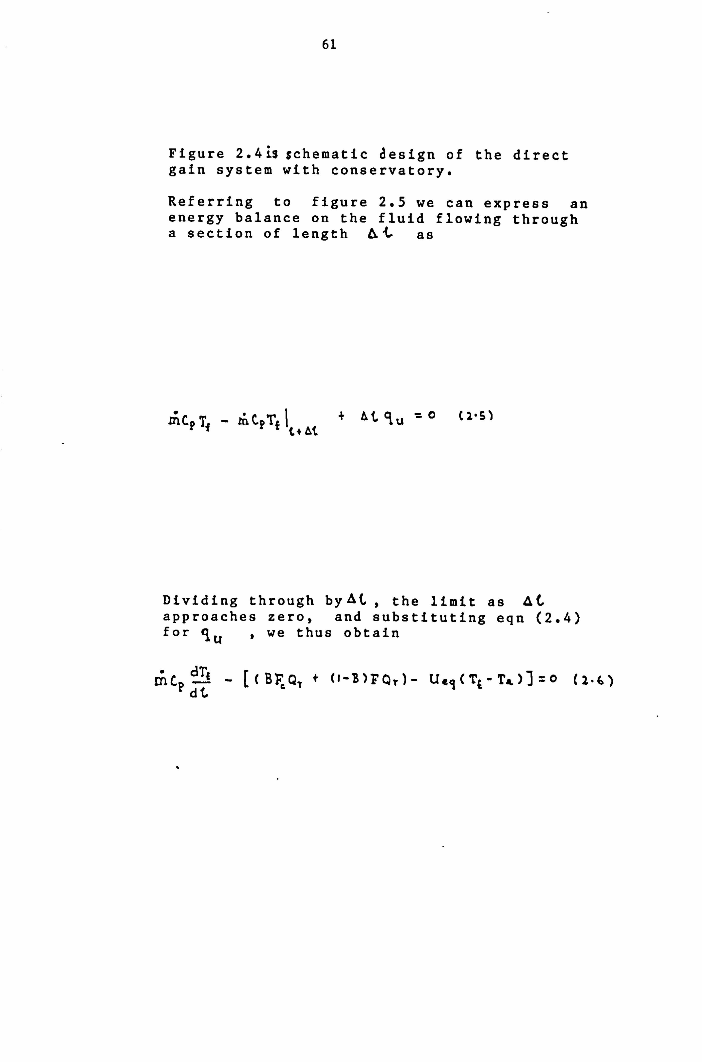
61

Figure 2.4iSschematic 8esign of the direct gain system with conservatory*

Referring to figure 2.5 we can express an energy balance on the fluid flowing through a section of length &L as

JAC, T, - 1ý C' Tj I t+ At

+ at qu -0 (2-5)

Dividing through by, &t, the limit as 4(, approaches zero, and substituting eqn (2.4) for C1. , we thus obtain

rýc LI

- [(BFcQT + (1-'B)Fqr)- Uej(Tj-T&)jýO P dt

61a

Tic r

TC Tal

"0

C0 -7 qr -T TC

lenglht L

Figure 2.4 Schematic Design of the Direct Gain System with conservatory

--b- s, ýerTi ij 1 -i->

Fig 2.5

FLUID FLOW (AIR)

Energy Balance on Fluid Element

62

If we consider that the equivalent loss coefficient'We. for the direcA gain system plus conservatory is independent of position, L) then the solution for the temperature at any position i (subject to the condition that the inlet fluid temperature isrr =T

is Csee section A. 18) for solution. fA 'CO

Tt - TA - (BF,, QT + cj-s)Fo. T)jUeq = r1UeqtliCp) T- Ta. - UCCI

cc, STC (IT

(2-7)

If our system has a length L in the flow direction, then the outlet fluid temperature

Tf-0 = Tc , is found by substituting L for f in eqn. (2.7) above.

2.1 Direct Gain System (with attached Conservatory)q Heat Removal Factor, 71ý and Flow Factor F"

It is convenient to define a quantity that relates the actual useful gain of our system to the useful gain if the whole system were at the fluid inlet temperature, Tf., j - TcO Mathematically, the collector heat removal factor, is then

FA Ck. Tco -To. ) UOCICTCO - Ta)j

i. e. what conservatory gives to ambient atexit is the solar input it receives at inlet minus losses (from building envelop to ambient) times the F

B

where i is the mass flow rate/metre square of cross section area. From eqn 2.8 the collector heat removal factor is expressed as

tý C? T, o- Ta I . 1.7B; F Qr Ua Ueq

4_

(2-9)

63

and from equation (2.7) when 'u- - L; i. e. the considered flow is at exit s and; for building envelop that flow ceases to receive solar gain; we can then express FR as

F. - 4, r- P, -e R U'jCI

Ii

or withý in J<SIs of flow cross section area we obtain,

(Ueq CP Ix "II

U eq

From eqn (2.11) the systems heat removal factor is a function of the single variable Uej / ý, C P0

In eqn. (2.11) j is the flow rate in the direct gain system by either infiltration or ventilation (stack and wind); in the flow direction per unit flow area (cross-section) i. e.

In infil ( -iniatration )

"' vent

(Vent! lation ) e2-1 . 2)

and ýI inal ; rh Ve'nt

are measured in J<g/Sm L

As the systems heat removal factor is a function of the single variable(U,, IinCI), 'a graph can be plotted of F.. VS Up,, Ith ni To fully appreciate the significance of theý curve, it is convenient to re-examine eqn. (2.8), but in a slightly different form.

Q= -F,

64

where QU is the total useful energy gain of our system. With this equation the useful gain is calculated as a function of the inlet fluid temperature. This is a convenient representation when evaluating solar energy systems since the inlet fluid temperature is usually known. However, it must be remembered that losses based on the inlet fluid temperature are too small since losses occur all along the system and the fluid has en ever-increasing temperature in the flow direction. The effect of the multiplier, 'p,,, is to reduce the calculated useful energy gain from what it would have been had the whole system been at (TE., j= T,

. 0); to what it actually is using a fluid that increases in temperature as it flows through the system. As the mass flow rate through the system increases, the temperature rise through the system decreases. This causes lower losses and a corresponding increase in the useful energy gain, since the average system temperature is lower.

This increase in useful' energy gain is reflected by an increase in the systems heat removal factor as the mass flow rate increases. See eqn. (2.11).

From eqn. (2.13) above

Jj6 F qý -i. ci - 15 tt (T4, it p

,a -t!. O.. c

[( g p.. %+Cj- 5)_F

-r IQ Fp- LQ AAV 4+ -r F

Fr. tQ4o. -tl -

. -A 0- rI-L. L. tL-)

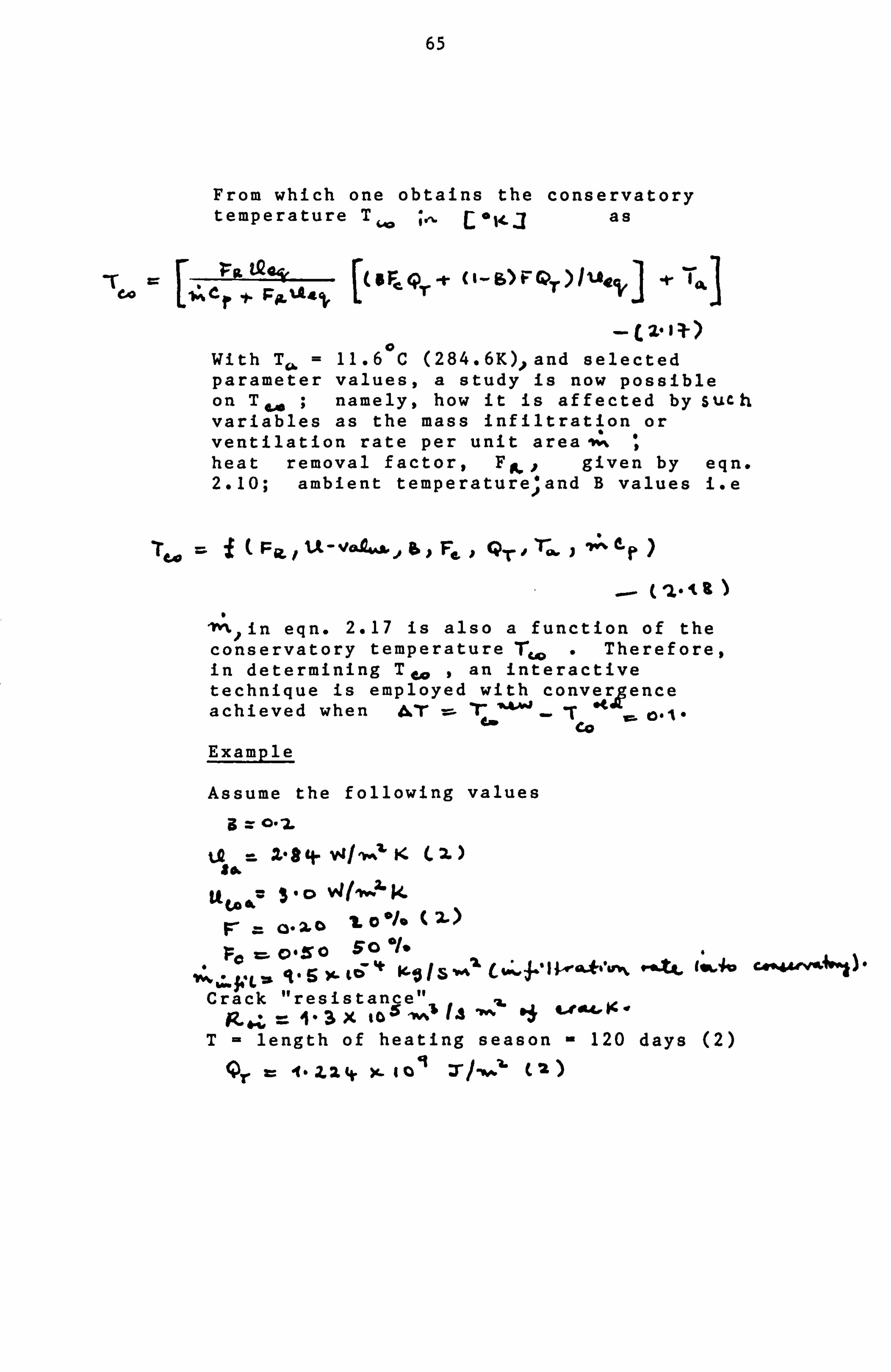
65

From which one obtains the conservatory temperature T,. ;-10 le- 3 as

roL tQ4v, (eF,, FQT L-, ýCj. * ;; jL%keeý

[

- E2. I I-)

With Tlý, = 11.6 0C (284.6K).., and selected parameter values, a study is now possible on T 0,0 ; namely, how it is affected by sue h variables as the mass infiltration or ventilation rate per unit areaw:, s, heat removal factor, Fp

. j. given by eqn. 2.10; ambient temperature; and B values i. e

vaL*. ä, 161F, , Qr. - 'r-c� , 41 0-? )

, rl-la) lr, ý,, in eqn. 2.17 is also a function of the conservatory temperature T,,, . Therefore, in determining TC, , an interactive technique is employed with conver ence achieved when &Y =:. 'r %A-Vj - 4M CO Example

Assume the following values ig = 0.,; L

tA = Z. 9 4. VJ/ Iv^21 KCI) S&

CA d6

'0.2, o, C). 50 %. 5Y

Cra"ck "resistance" q6 9" = 1.3 9 to 5 M$ -W.. 4., faA,

T- length of heating season 120 days (2)

Iýr = It* Z24 Y- 1 10 41 2- / ovv%"&. ("

66

Evaluate the heat removal factor for the above direct gain system with attached conservatory (B = 0.2), a quarter the size of the room; using eqn 2.11, assuming C. for air is 1012 J/KgK and ambient temperature Tc%. of T ,6= 11 .6

43 C (284.6K) (2)

Solution

Eqn. 2.11 gives the heat removal factor for the above example.

;: =;, CP eC AU 4LAV

Using eqn. 2.2.5

tA4A A. 4 -r 9 u'. . -a -a -11 wl-ý, v-

r . 50.46 0, ) -(. W

4) 4(zz) IL,

. jý- Fr it.

Now, evaluate the temperature of the conservatory for the above given conditions.

Using eqn. (2.1-+) T La

is in degrees Kelvin given by,

0-01+4 2V4-6

67

Evaluate Q Ir in W/-i. %I' day using Q-T (120 days)

=1-1Z gf x %, 0 q(t2. t Je -td )(2. )

C. I ZA. 4 x taýo

ýLO X 'L+ jx JGWO w Iv.; L Q . -T -

= va - A-T

-

4 o-o4ý4(44&so) + ; Lb4-*fO

CIO

or T"

0. This is the average conservatory temperature during the heating season (120 days), using data in ref. (1,2) and the above analyses.

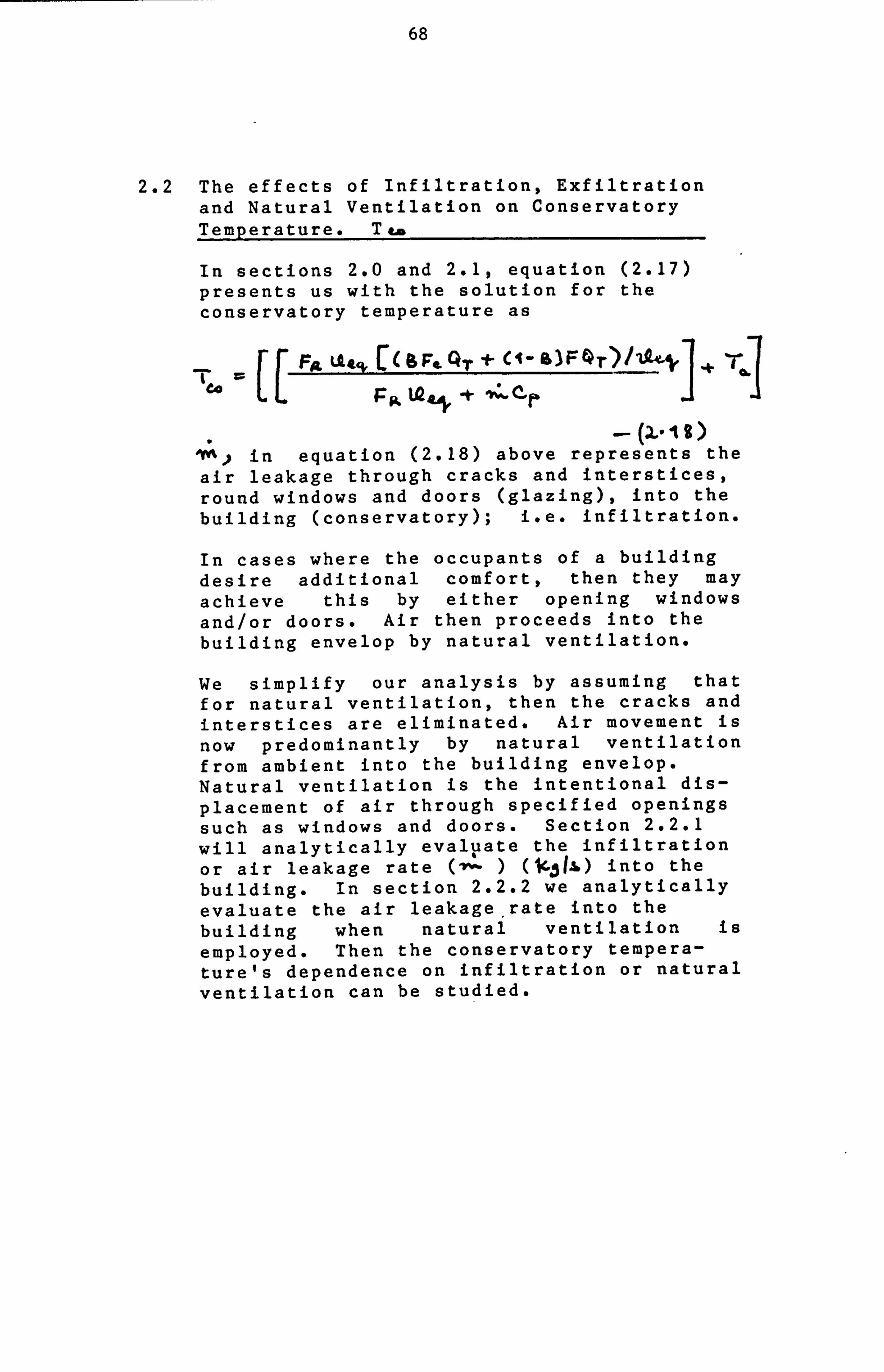
68

2.2 The effects of Infiltration, Exfiltration and Natural Ventilation on Conservatory Temperature. T"

In sections 2.0 and 2.1, equation (2.17) presents us with the solution for the conservatory temperature as

ua% C4a Fo. QT +CI-a3F lea

+

in equation (2.18) above represents the

air leakage through cracks and interstices,

round windows and doors (glazing), into the building (conservatory); i. e. infiltration.

In cases where the occupants of a building desire additional comfort, then they may achieve this by either opening windows and/or doors. Air then proceeds into the building envelop by natural ventilation.

We simplify our analysis by assuming that for natural ventilation, then the cracks and interstices are eliminated. Air movement is now predominantly by natural ventilation from ambient into the building envelop. Natural ventilation is the intentional dis-

placement of air through specified openings such as windows and doors. Section 2.2.1 will analytically evaluate the infiltration or air leakage rate (-#ý- ) into the building. In section 2.2.2 we analytically evaluate the air leakage, rate into the building when natural ventilation is

employed. Then the conservatory temperature's dependence on infiltration or natural ventilation can be studied.

69

2.2.1 Infiltration Air Leakage Rate into Building

Air flow rate into and out of a building due to either infiltration, exfiltration, or natural ventilation depends on the pressure difference between outside and inside; and on the resistance to flow of air through openings in the building. In this analysis we consider the configuration between ambient at Tc,, and room air Te as shown in Figure 2.6.

The amount of air flowing through a crack in an outside wall, window or door, depends on the size of the crack, and the pressure difference between inside and outside.

In most cases, the resistance to air flow within the house is negligible. For the purpose of infiltration calculations, the house can then be regarded as a box, as shown in Figure 2.6.

For all types of windows and sliding glass doors, the Federal Mobile Home Construct- ion and Safety Standard (Fed. MHC SS 280.405), see ASHRAE handbook of fundmentals (17); presents the infiltration through cracks as

or

PC In eqn. 2.20, pVis the weight flow from 0 to ( Ica /4Aa); A. is the air leakage &*-tftC-a)e

P... static pressure at b (see Fig 2-6); vj the flow exponent (usually n-0.66 (18)), and Ca flow coefficient.

69a

lýe£ er enze I'Side

0'. Lawel ier a .

a a0 . cl

Fig 2.6 Illustration of Infiltration into building from ambient

69b

140

-A

L4

X

3 0

A16,3 -0

pLe; 17 ) -X

Ratio outtet to inlet ato-a- or %iir-P, -Vers&

Fig 2.7 Plot, Predicted vs Monitored Air Flow rates increase, resulting from unequal entrance and exit areas. Eqn. A16.3 (Predicted) (Ref. 17) (Monitored)

69c

3 aL It :L -d a va

C4

ct

dr t4

Ci

e%uc . -%

P. 0t " i

% . i dlý %

:

li oý

3 b% u1» $ _d .Z 4

%0 N 4 j 1

, ., I

S.

I

ri

Lu

. 01

-* %0 IA

'I 0

4C6

,; LU

to 0

Co Co

ýi Co

rA 4 41

bo -H

Zm u >%

r-4 U)

w Co 00

4.4

0 1-4 0

wH 41 bo P CU

to w r. 00

Co 44 u 0 %.. ý

0 :1

w to

w0 pw 44 0

Cl

iv dý

., % 11 c;. t

70

Equation (2.20) can be rewritten as

P4

eý=e I It'OL

where *04c, ý is the resistance of the crack, defined as the volume flow rate per unit area of crack, at a unit pressure difference. ASHRAE handbook of fundmentals (17), gives for all types of windows and sliding glass doors

% 3' /s bk, %7- o-j v= OOXS4 ,

at pressure 75 Pascals (Nlw%X ),

equivalent to 11.2 m/s (V W wind velocity pressure.

Evaluating the Crack's Resistance to Air Flow

We proceed by evaluating the "resistance" of the crack for the case considered i. e.

"all types of windows and sliding glass doors". Reference is now made to Figure 2.6.

The static pressure at point o in Figure 2.6 is given by

C. *e V

where ASHRAE handbook (17) gives the wind pressure coefficient C* for elongated rect- angular crack at T,,,. = 11.6*C as C4ý-

S1; 0

Its, is the density of outdoor air (*Kg/m Vw the wind speed (m/s); L):, - 11.2 m/s; g the gravitational acceleration. g-A0 94 " IJ'6

and the distance between reference levels

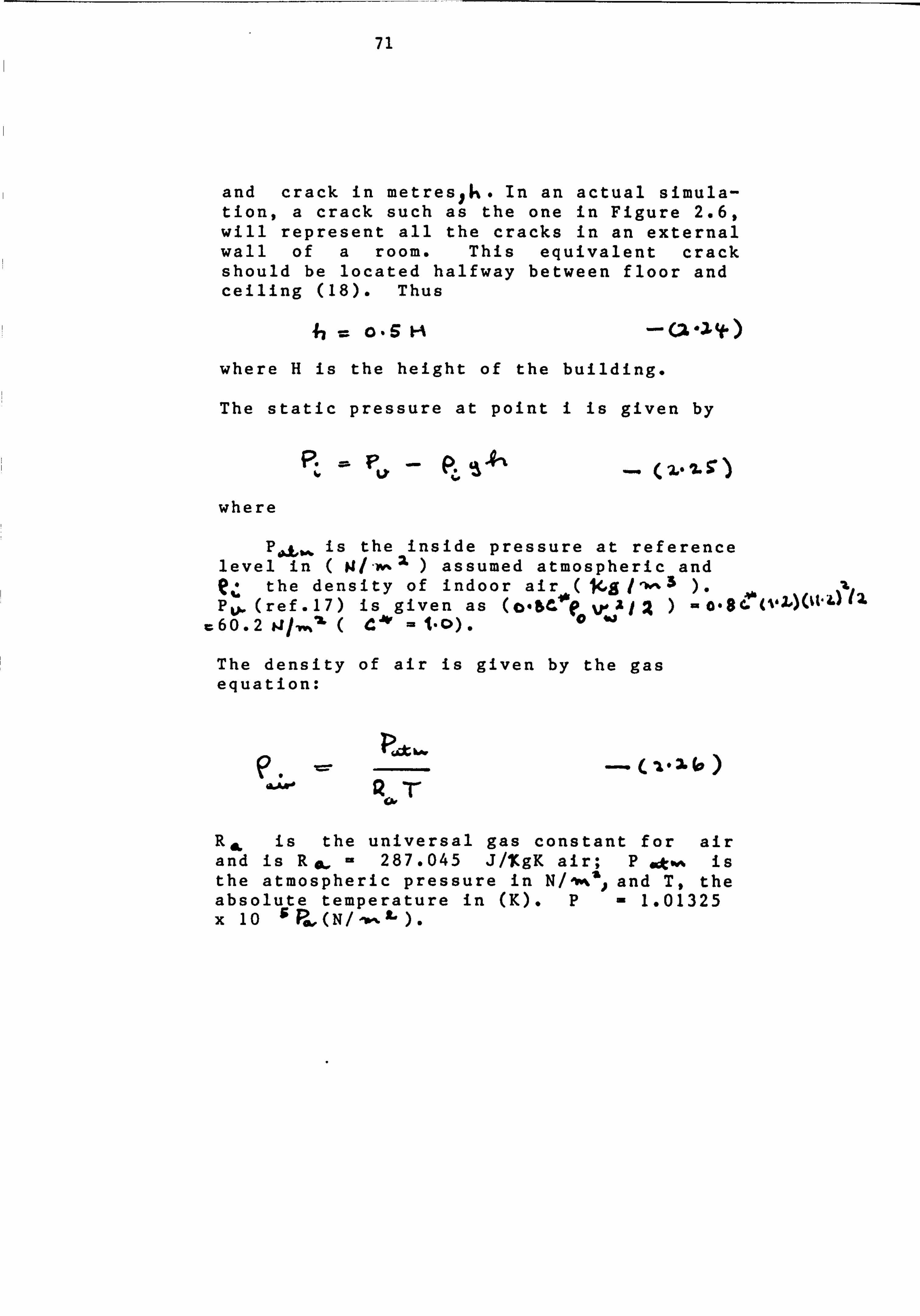
71

and crack in metres)k. In an actual simulation, a crack such as the one in Figure 2.6, will represent all the cracks in an external wall of a room. This equivalent crack should be located halfway between floor and ceiling (18). Thus

ýh = - (. 2 -3, ý- )

where H is the height of the building.

The static pressure at point i is given by

p. p- �. 7

where

P,,. L.. is the inside pressure at reference level in ( 14-w-1 ) assumed atmospheric and

ez the density of indoor air ( j4S 1 -ow%, S ). % Pw (ref. 17) is given as WAI :t)-

c60.2 9/vv%*& ( e. '* - 1- 0) . to

w

The density of air is given by the gas equation:

F Pat I., OAR' QT

R& is the universal gas constant for air and is R&, - 287.045 J/%gK air; P "t W% is the atmospheric pressure in N/, r. %s., and T, the absolute temperature in (K). P 1.01325 x 10 5 Pe, (N / -*% IL ).

72

From equations pressure diffe can be written

(2.23) to (2.26) the rence 61> ý, P,, of eqn. (2.21)

as

T"', Tcý

-CZ- 2 1)

where T,. is the outdoor ambient temperature, To_ = 11.6 c' C; and T c. the indoor room temperature, T r. = 18.30C.

From eqn. (2.21)

From eqn. 2-2Z$2-11,,, for V,.., = 11.2 W%ls n=0.66, C* = 1.0, the crack "resistance" R,,, ý is evaluated as

Rf *0 - PZ -( (0 145

0-1 C*- T, % Tc,

In using T 416te-

in subsequent calculations

[K] ,( 14, 'To.,

e

and -ca. at)

V_j Te, T,, 4-1 1 ps t6 0

From eqn. (2.30) c

)l TIZ.

where VW - 11 .2 and 0. 00254 of A. (ref. 17).

73

6 Evaluating the Air Flow due to rAr

To evaluate the weight flow (air leakage/ infiltration rate) in XtIs-v-l'of Aa we use eqn. (2.29) and. (2.30). From these two equations, NI is given by (in I(g/a -u, 4 of crack area A

Aa= &( 4ý-Z ) the inlet area - (length y- clearance of windows) x no. of window lengthsinvolved. Then

o-66

C. L) 0"5

cc V 2. ) POX.

For a crack area, A. the weight flow or air leakage/infiltration rate in Xg/s is (2. "54) then given by

I)I %X - a-616 ' ! '* ýL ý, O'%C-

&tow.

R,, C.,

2. rCL TC. ILCk,

Co. I-S, j

In evaluating the infiltration rate from -2. S. 5 eqn. (2.35) above the wind pressure coefficient C* depends on the atmospheric temperature as well as wind velocity VW For T 0, = 11.60 C and a windspeed VW 1-L

'W. JS C11L is obtained as eft, 1.0

74

For various values of T,, in (K); see ASHRAE handbook owý& Product Directory (17).

pt. "

c

c -W must be evaluated from eqn. (2.36) for a given ambient temperature; before us in eqn. (2.35), with T. in QA). VW in the numerator 4 eqn. (2.35) is not 11.2v-/, s, but the pertinent value at the location. H= height of building.

Sample Calculation

1. R Crack "resistance".

Substituting T,, = 11.6 0C (284.6K) in eqn. 2.36 gives C* as

C, #- -s. 4- In 0. cl

For Ow'= 11.2 m/s. *This is not the input for V,,, & in the numerator of eqn. (2.35) for

but the pertinent speed must be used.

00 T .29 K-

cin 2-3tp) ,, = 11- f. *e- = 2. go+-(. K (Lc,,., 4. *crn t4. ac. V-

la, C" C. 14 C, 1ýr. -

( Tý, > T.,

P'tt. %

=4ot32.. 5 ?, -

Substituting the above values into eqn. (2.33) yields the "resistance" offered by crack to air flow as

75

ýe oL =ý

ýý- I[ *-I XJ. jý Y. C44-1)ý

_ 4-11-114 1-I

2.8 4- - 6.2.

(L14*L xdtj. 3)]

Co. 00; L. 74_)

Izaz p1t.

P- ".

I

For a building of height H 4m,

't o13 *2 S' I/ -, ý [64-V3, t[I 17# 0 (4-S

I -iv-w

Or R=i, IA to 57

IV^ 'I Is IVWI. "6 1 X,,, -CZ*4'0)

Eqn. (2.39) indicates that as the height of the building, H, increases, the crack "resistance" to air flow, RL , increases. This is to be expected as the increased gravitational forces in a taller building should increase the-"resistance" to air flow by the crack.

R" can be plotted as a function of the building height H in (m)

Calculate ý41.

Eqn. (2.35)

From eqn. (2.35) assume a wind speed of 5 m/s. (The pertinent value must be used in the numerator of eqn. (2.35). Hence,

U. =s'. Is vi

76

Assume H=+ %Vl 4; ýt&^ = -t ai IS 2T Pe, L%a -%x )

-4 a.,, O 6-ý 4it--. Z- 3 16 ) -, [ Oleýl t1ti ah.

C. V- Cý ) -act ') 2. - 3 (a Cý f-0

-; 6 it 4. (. " y-

Trý YCg )=I Then from eqn. 2.35 forlý and 2.38 for

0. &k

Pt. 1.0 O.. rxf-al xe-i. ? bt.

ka Tr2. % 4

(219'e.

6 LII. 3 go,

1

4. LI C ýi

, 4- 3 x. Lt) 5

t- where

-ce c=

1-i-,

t

In this case TTe. =2 91.3K (T > T.. Then,

I Cý 3y. '10 -1 -jL

'L 67.04. r

"'I = 9-S I C; 3

77

Assuming that the glazing area constitutes 3 windows/doors of size (1)(1.5 m) and clearancet6lm; then the leakage area/flow area A is given by

Ab, a[( 't Y. it; ') x 2. *(A. 5 Y.

3 V. 0.05

-4 .0 -4- From which-; 4 becomes 0.00014 Kgjs or 9. ýJ&*Ar

Hence the infiltration or air leakage rate

,M= C1 . Lt, XI Cý 4 14,5 1 S. &: Ir VV%1 &ý 4U VJ IA. 4-f-(X 0

M- (2. **L) This value of vý is now used in eqn. (2.18) for T.,

74.. =[ --FA -IA, @, L, [c, 3F, Q-r -r(A- ia) F(ý-)/Uftj ],

-%,, I

j: j;. U. C, -i- -VZ, 0- F

I

V, -

where-vý is as calculated above, i. e.

- q. q.. )( Io Is -' c'-. ttcrJ '-o. I

-(

2.2.2 Rate of Ventilation Air Flow into Building., ;. by (A) wind and (B) Thermal Forces- v C., -L-

It was pointed out in section 2.2.1 that, when natural ventilation is employed in a building, i. e. the occupants desire additional comfort and open windows and doors, infiltration flow is superseded and the term, 4, in the eqn. (2.43) above for T..,, is now-A,.,,. t for the building envelop, wt.; cZ, following recommendations in the ASHRAE fundamentals Handbook (17).

78

Air movement into, through or out of a building may be caused by wind or thermal forces, acting alone or together. Arrangement, location and control of ventilating openings should be to combine rather than oppose the two forces. In the following section the air flow in due to

Wind and

Thermal Forces

shall be evaluated for our building envelop.

(a) Flow due to Wind

Factors affecting ventilation wind forces include average velocity thj , prevailing direction, seasonal and daily variation in velocity and direction, and local obstruc- tions such as nearby buildings or hills.

Wind velocities are usually lower in summer than in winter; frequency; from different directions differ in summer and winter. There are few places where velocity often falls below half the average. Thus, natural ventilating systems are often designed for wind velocities of half the average seasonal velocity, i. e.

4r) & "A-0 r%

where V,, 3 is the design velocity and USA4",

is the average seasonal velocity (120 days).

Eqn. (2.4 6) below shows the quantity of air forced through ventilation inlet openings by wind, or determines the proper size of openings to produce given air flow rates. In

79

tr. =- 'Z L>, t ( ii 3)

W% 1. c9

-(a. - 44- (. )

where 1)'. Is the air flow in A is the free area of inlet openings in square metre; Vw is the design wind velocity given by eqn. (2.45) in '1, ^IL ; and Z the effectiveness of the opening. (Z is taken as 0.50 to 0.6 for perpendicular winds and 0.25 to 0.35 for diagonal winds (17)) i. e.

0 -. 5 Ir x :! L- a-6 perpendicular winds -(a. 4-, 4- )

25 :S 12 & 0'3 S; diagonal winds

In these computations the effectiveness of the opening will be taken as

Z=a. S( EcbDlo )

Inlets should be directly into the most frequent prevailing winddirection. If they are not advantageously placed, flow will be less than that from the equation; if unusually well-placed, flow will be slightly more. Desirable outlet locations are

80

(1) On the leeward side of the building directly opposite the inlet.

(2) On the roof, in the low pressure area caused by jump of the wind.

(3) On the sides adjacent to the wind- wards face where low pressure areas occur.

(4) In a monitor on the leeward side.

(5) In roof ventilators; or

(6) By stacks.

Flow due to Thermal Forces

If there is no significant building internal resistance, and assuming indoor and outdoor temperatures are close to 27 0C( 80'6F ), the f low 4%. - lfý S(S

.1 due to stack effects is

ý4+ ML& V_ = VR AC -004 (Tc, --rL xIC; *

whereý (

., t,,, V. is the air flow in A., the free area of inlets or out-

lets (assumed equal) in square metres; 4'-J the height from inlets to outlets

in metres andt may be assumed

, &tj = 0.5 H-cI. ra )

where H is the height of the building for a window located midway between floor and ceiling, assuming outlets employed are stack outlets on roof as in Fig. 2.2 -T r_ is the average -46-r'e temperature in (OW. ). Irct in equation (2.49) is the constant of proportionality, for an effectiveness of opening Z=0.5. n.

, a, - sa A.., z -t"-r . : __ Cs. y).

81

Greatest flow per unit area of opening is obtained when inlet and outlet areas are equal. Eqn. (2.46) and (2.49) are based on their equality =- Area of glazing, window or door. Increasing the outlet area over inlet area, or vice versa, will increase air flow but not in proportion to added area. When openings are unequal, the usual practice is to use the smaller area in the equation and add the increase in flow percentage) as determined from standard curves. Reference is made to the ASHRAE handbookof fundamentals (17).

(i) Flow due to wind forces, or thermal forces (Increase)

o-17 As.. x

JOD J*, tu. KAZ -r= 0- 94 -( tz. ". e

where A,,. tand A.. are the outlet area (stack area in roof), and inlet area (area of window or door in conservatory). The correlation coefficient for this fit is obtaAned as 'ý-= 0"14 - Actual values of (AVw )

obtained from the curve in ref. (17)

and those generated by the fit in equation (2.51) are presented in tables 2.1$Fjg. 2. jo, for various ratios of i. e. outlet to inlet flow area.

When one uses equation (2.51) and equations (2.45) - (2.50), Vt,:, CL and are then evaluated in terms of the ratio of. outlet to inlet area A 0,, x / As. . V. ý, g the air flow by ventilation due to wind forces in-r"/. S is then from eqns (2.51) and (2.45) - (2.48).

82

; Vý

-(2... S* 1)

Using an effectiveness of opening of 0.5, and the wind velocity as the average season value ( .1) (- I S)

(ii) Mass flow rate of air forces (Ventilation)

From equation (2.52), rate by ventilation d on open windows/doors

due to wind

Y; % A

the air mass flow ue to wind forces

simply becomes

e vw &kn 'IQ

and V,. J;,. ZL ,4 YIýL-

x to S

A6

*-S7

j -j- - 14- 1r tl--r

- ') AL

.5

where

-4A

, e. �. z -z AL ý -lý - (1. -946)

,C

83

u9.4A n

- (2. cq-&. )

P is the atmospheric pressure, O*F,. and R,, is the universal gas constant for air, ( IZ4 = 2. S'7. cb*S' Tj ; ý5 V- -Z4- )- T,, is the room temperature set at ( Td. -I it *3*c E 2L'I 1,3 "K

.3) and T, -the ambient temperature.

T,, the average heating season value ref . (2) is -rm w 1.1. GOc r_ xv4.. r, k. 3

Mass flow rate of air due to thermal

_forces (Ventilation)

IVU, ct,, &V-

Similarly from equations (2.51) and (2.49)- (2.50), the ventilation air mass flow rate, due to thermal forces (stack effects), (i. e. temperature differences between building envelop and ambient);

6.31 -P

9 Z' 44 ij'Tc -

e' , CK

Or

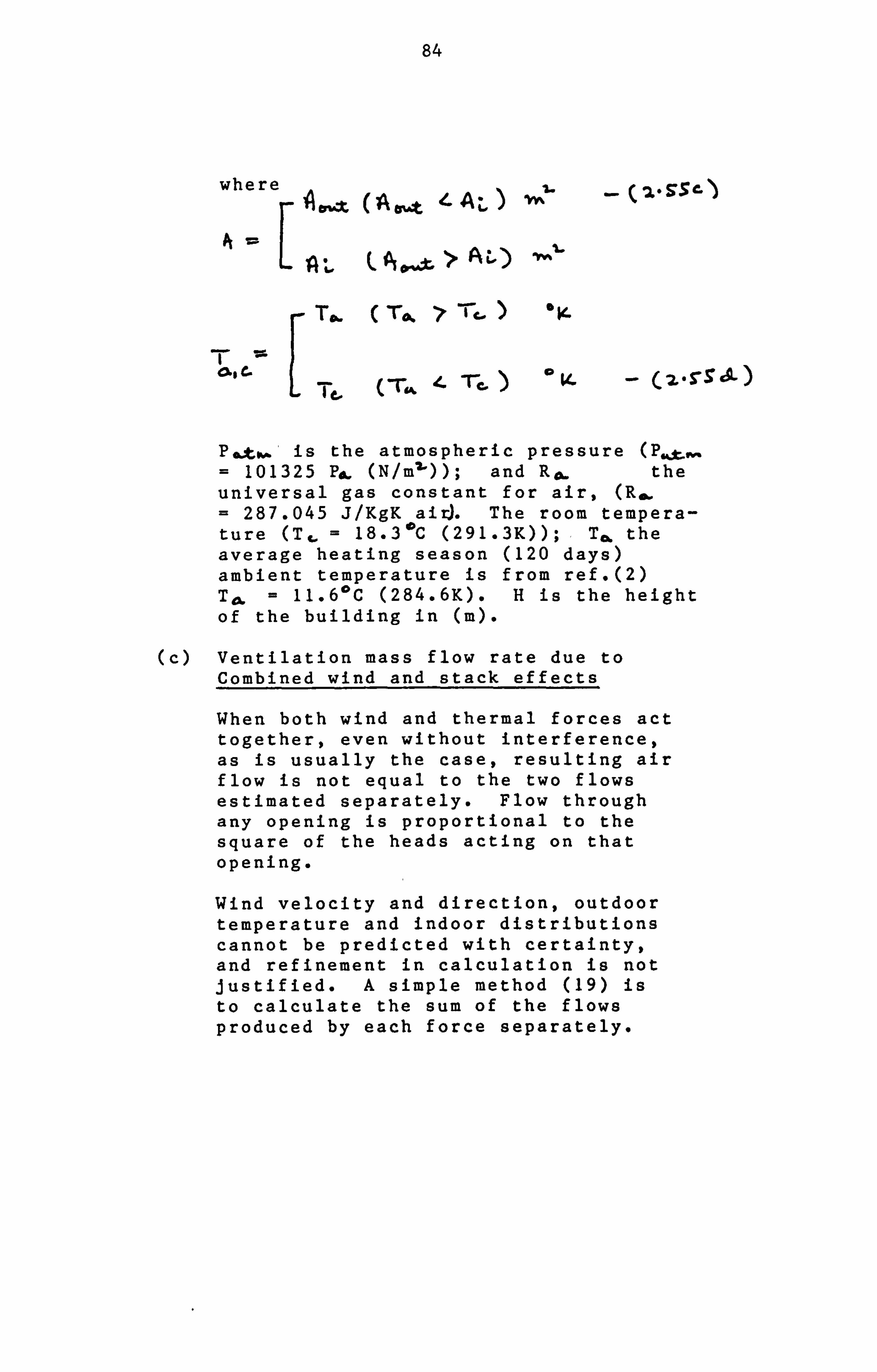
84

where 16. Ot Z- AL

'A L>A

T,. To. *7 Tcý

I= 06, Cý

-- rm V-

ý It,

Po,. tv,. is the atmospheric pressure (Pt-,. = 101325 Pa, (N/m2-)); and Ra- the universal gas constant for air, (R,, = 287.045 J/KgK air). The room temperature (Tq, = 18.3*C (291.3K)); T.. the average heating season (120 days) ambient temperature is from ref. (2) To. = 11.60C (284.6K). H is the height of the building in (m).

(c) Ventilation mass flow rate due to Combined wind and stack effects

When both wind and thermal forces act together, even without interference, as is usually the case, resulting air flow is not equal to the two flows estimated separately. Flow through any opening is proportional to the square of the heads acting on that opening.

Wind velocity and direction, outdoor temperature and indoor distributions cannot be predicted with certainty, and refinement in calculation is not justified. A simple method (19) is to calculate the sum of the flows produced by each force separately.

85

9 Im W- UU-tj , ý. 09 ttci- V-

Then using the ratio of the flow produced by thermal forces to the aforementioned sum, the actual flow due to the combined forces can be approximated from standard curves (17) as a multiple of flow due to temperature difference. A fit on this curve, see A17, yields the actual flow as multiple of flow due to temperature difference; a function of the ratio

-fýV4. ZI &k ow. V- f»toi-v- >t. -t j . *.. .0) The multiplication factor on

V- that yields the combined air mass flow rate -#ý, .t., ý V., .a is empirically evaluated in A17. The air mass flow rate in (Kg/s) due to combined ventilation., wind and thermal forces can be written as

355'S' I. ct +4

.; 1.

are the ventilation air mass flow rates in (Kg/s) due to thermal and wind forces and are given by equations (2.55a-d) and (2.54a-d) respectively.

A correlation of Y- - -0.97makes such an empirical form attractive where

-ý, wt, * 0 V. i Vý- , týo .0-

85a

CY IN (9 r. w 0

9 m 4 *A

W 44

v» 1:

0 c:

0 4)

to (0 >,

10 j2

3: 0 ,q 0

41 44

44 0 :i

0 10 0 .

0 :1 44

10 01 0

19 -H 9) u

w 0 u

0 44

9

ci 000 (2 9 ll; Ci 19 ti 9 Ilý r4 c4 ty 00 W. 4

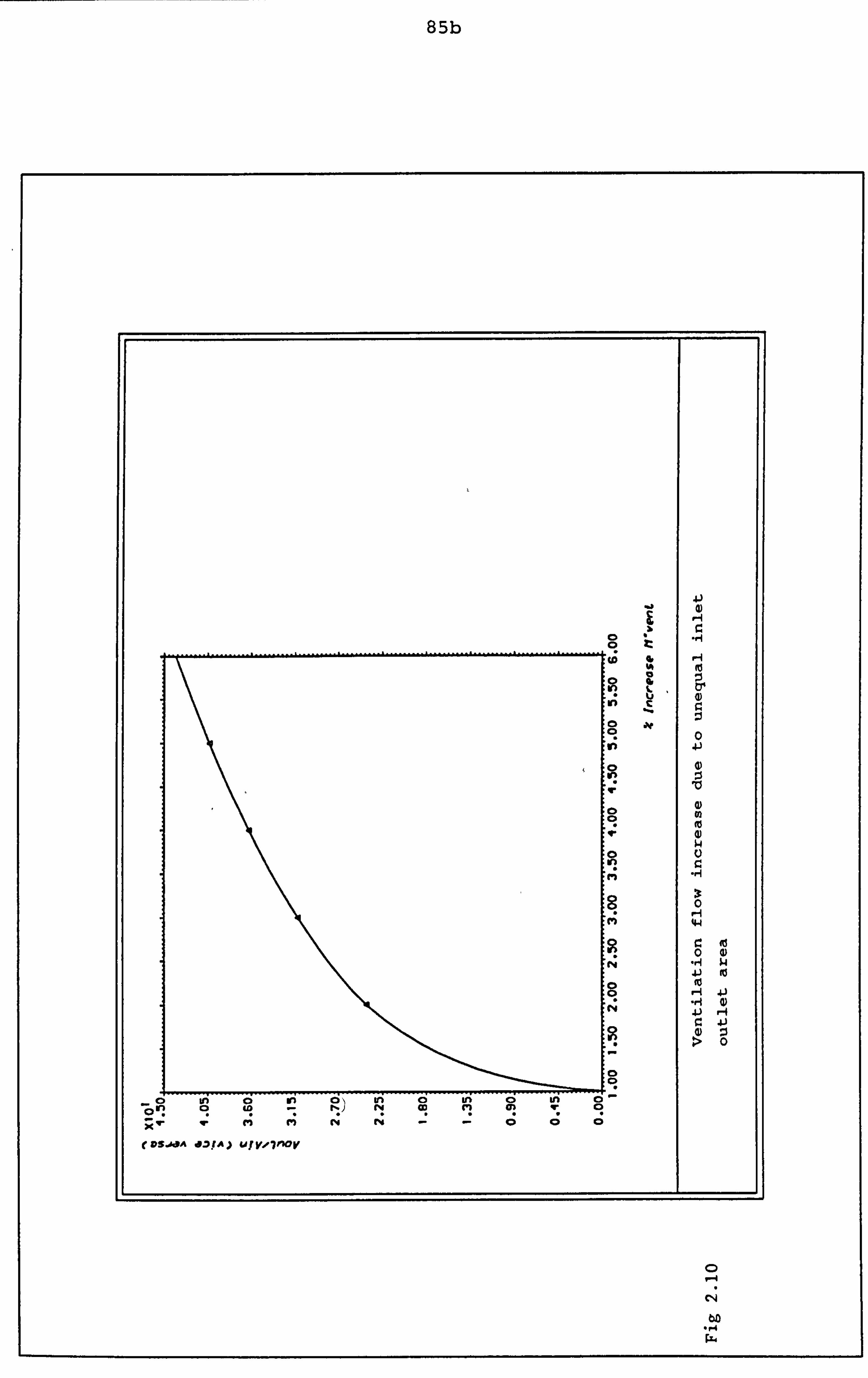
85b

4J

..................

0 C! ý 4J

w

0 11 0

-H 4) 41 4

0

0 In ci in 0) tn a 99 11: ri 0! Ln 6 L6- 6-

C! a! V; 9 wm cn 914 N- 00

VS. J4A 9. 'J. tA fd/ve7nov

C) 1ý N

6D ., 4

86

Thus, when ventilation is activated in the building by opening windows and doors by the occupants, the combined ventilation air mass flow rate into the building is given by equation (2.66) above. Infiltra- tion effects being thereby superseded and vice versa. The eqn. (2.18) for conservatory temperature then becomes

1 to =1[.

rg. t'eý -- -rUrt, tx. �ýv.

CO.

-

-( 2--61-)

where the heat removal factor is from eqn. (2.11)

CP

Fit ; t,

2-b and the equivlant heat transfer coefficient for the building envelop Ue_V from eqn. (2.265) ZA

=(4-a) lts, ý.

'LL2,0". - (2-1 (aft)

In equations (2.67)-(2-69), T&,, is the conservatory temperature in ( 4K ).

B the volumetric proportion of air (from unity) retained by the conservatory. 0 -B )is retained by room air at a temperature Ta_ f ixed at (Te- v- 42*3 C ( tilts 6 K, )). The fraction of transmitted insnlation (QT '-- 1*22* (2)) not absorbed by conservatory *... 9

storage in room; which directly heats the air in the conservatory and room are represented as F. and F respectively.

87

Tvý 0

is the ambient temperature, T,, =. 11.6 C (284.6K); Ný% vent, stack, wind is the ventilation air mass flow rate in (Xg/s) due to combined wind and thermal forces as in eqns (2.54a-d), (2.55a-d) and eqns. (2.66). Cp is the specific heat capacity of air at constant pressure, P. Z 101325 ( fa. so. rj/,. '*)

,Cp- 1012 J/%gK. FIL is the equivlant heat removal factor for the building envelop (ratio, dimension is the equivalent heat transfer co: f)iiUcLi*e"nt for the building (W/ %v% 2- KL is the length of the direct gain system in the flow direction (eqn. 2.12), (L - conservatory depth 4- height of room)(m). U "#& I heat transfer coefficient from conservatory to ambient ( 3-0W/w0' K U5, A , heat transfer coefficient from storage at room air, assumed AA;

L. a Usok T. - I *I (WI Nv%"- V- ). U96, heat transfer coefficient from room air to ambýent, 11 j c,. - 2.1 9 LiF W/ 'w%, " V- L r'44 1 :1

M (vent, stack)is the ventilation air mass flow rate in (Kg/s) due to thermal fo. rces as given by eqn. (2.55a-d), and

M ývent, wind) the ventilation air mass flow rate in (%g/s) due to wind forces as

given by eqn. L2. -S4a-d).

Sample Evaluation *-j Ventilation air mass flow rate (Kg/s) due to combined wind and Stack Effects

Air Mass flow rate due to Stack effects ( k:, - , Lt-4ý 4

Equation (2.55a-d) gives

40 AX 241 ± ew! tS V- 4- iýsy. t-36

I'S 7-C 4-'S A 2,11 3

88

41 0. *0sC vl, ̂ Zj st" LL

4eS I C_ -, -' 01 -9-ýl "I '

where;

assuming inlet area is four times outlet area, A &At/A Z or vice versa assumes a numerical volume Of 4 -Cre -T t. c.. ) (Te -? To-)

t-I .76 Te AI- IS oc- 3 V- ) C- -C! Q

'r,,,, 24 V- T, 6-I-

a X,: t , ýr 4ýr,

IA= 0'25)t 3,

cs

a.,, Q

0-251 -00-C

Air Mass flow rate due to wind effects

Equation (2.54a-d) gives

04 3"A 5x0 -S' x0 ; -. 5 A )L 1.36 21? 7-04+. r ; Llq(-3

a-0031CV-8/5) 'aw C16004 JQ C> 4-

assuming the same conditions in 1 above including an average wind speed Lt-

a %, a r%

89

From the above example, the increase in ventilation rate due to unequal outlet ý-LO-t

area (A L/A*,, &- 4) and an inlet area of 3 wind&Ps(l x 1-8m), At - 3xl. Om ia36%. (4-3 G 44, ev. It is apparent too that th, e stack vent-

, ywind forces%%.. t,,,, Z,, 0.403kg/s, ilate rate)p b 4""rc.. ftj, a^A = 0.0031 kg/s for a wind speed of 0-ý, & -5 m/s and air of density 1.2 Kg/ml.

3. Air Mass Flow Rate due to Wind and Stack Effects

From the sample calculations 1 and 2 it is apparent that

t; ý, WC%tO sta. L V- Ci It *It,

044--Z, S&O. CýW- ".. Z, . 4.9L i. e. th stack ventilation air mass flow rate is 99% of the combined flow rate by wind and stack forces.

The combined air flow rate is sum of the two flow rates but equation 2.66 above. Hence,

too L10.44-03

4- O-Cý02 I

L

not simply the evaluated from

11 1.19

1

çtcC14

=(I. o-+ ) ýA, V44%*- 0 14

90

Therefore, the combined ventilation air flow rate for the above example is equivalent to a 7% increase on 'VA(vent, stack)for a flow where stack effects predominate by 99% of the combined flow, and we obtain

41 0

OR

>ý 0- te 31 (l% 4ýr 1s)

"--e# N%wo. 93 v-

when ventilation supersedes infiltration, this is the value ofvt%. in the eqn. for T... and vice versa.

(d) Practical Considerations when Utilising Natural Ventilation

Types of natural ventilation openings include

(1) windows, doors, monitor openings and skylights.

(2) Roof ventilators.

(3) Stacks connecting to registers; and

(4) Specially designed inlet or outlet openings.

Windows

Windows transmit light, of course, and provide ventilating areas when open. They may open by sliding vertically or horizontally; by tilting on horizontal

pivots at or near the centre; or by

swinging on pivots at the top, bottom or side. Air flow per square metre of opening may be considered the same. Type of pivoting is an important consideration for weather protection.

91

Roof Ventilators

A roof ventilator provides a weather-proof air outlet. It is actuated by the same forces that create flow through other openings. Its capacity depends on its location on the roof; the resistance it and the ductwork offey% to air flow; its ability to use kinetic wind energy to induce flow by centrifugal or ejector action; and the height of the draft.

A ventilator should be located on that part of the roof where it receives the full wind without interference. If it is installed within the suction region created by the wind passing over the building t.. ' 6 1.,

L. 4(Atýbetween two high buildings, its performance will be seriously impaired and its ejector action, if any, may be lost.

For a high flow coefficient, the ventilator base should be of taper cone design to produce a bell-mouth nozzle. If a grille is provided at the base, or struct- ural members introduce resistance, the base opening should be increased accord- ingly.

Building air inlets at lower levels should be lax. ger than the combined throat areas of all roof ventilators.

Natural draft, or gravity, roof ventilators may be stationary, pivoting, or oscillating, and rotating.. geJection criteria are: ruggedness; corrosion-resistance; storm- proofing features; dampers and operating mechanisms; possibility of noise; original cost; and maintenance. Natural ventilators can supplement power driven supply fans;

the motors need only be energised when the

92

natural exhaust capacity is too low. Gravity ventilators may have manual dampers

or dampers r_ontrolled by thermostat or wind velocity.

Stacks or vertial flues should be located where wind can act on them from any direction. Without wind, the chimney effect alone removes air from the room with the inlets.

Generally, the following natural ventilation rules must be considered.

Buildings and ventilating equipment should not be oriented for a particular wind direction, but should be designed for effective ventilation with all wind directions, since very few places have prevailing winds. Even if a wind direction prevails 80% of the time, safe adequate ventilation is needed for the remaining 20%.

2. Inlet openings should not be obstructed by buildings, trees, sign boards, or indoor partitions.

3. Greatest flow per unit area of total opening is obtained by using inlet and outlet openings of nearCy equal areas. See Fig 2.7.

4. Direct short circuits between openings on two sides at a high level may clear the air at that level without producing any appreciable ventilation at the lower level of occupancy.

93

5. For temperature difference to produce a motive force, there must be vertical distance between openings; vertical distance between inlets and outlets should be as great as possible.

Openings in the vicinity of the neutral presssure level are least effective for ventilation, and

70 Openings with areas much larger than calculated are sometimes desirable, when anticipating increased occupancy, or very hot weather* 'rhe openings should be

accessible to and operable by occupants.

2.3 Solar-Load-Ratio Statistics in the United Kingdom

The original method of Gordon and Zarmi (1,2) did obtain close form analaytic expressions for the solar heating fraction (SHF) as a function of the solar load ratio. The analysis as presented by Gordon and Zarmi did assume the frequency distribution of daily SLR values to be parabolic about the mean. It was however recommended that the actual SLR frequency distribution for the location be employed in estimating the SHF values. Cowing and Kreider (20), in their study of locations in the United States, obtained the actual frequency distribution of SLR values for twenty-six cities in the United States. They showed that a fourth order polynomial proved sufficiently accurate in characterising all SLR values. The relationships was of the form.

SLk, + IC. 5. SLP. 't' bi L SLIZ

-(2. +c) )

94

Higher order expressions increa&t4 the complexity of the closed-form solar fraction expressions with only marginal increase in accuracy (21). Basically, the work in (20) presented the following improvements on the original Gordon, Zarmi (Gj7. ) method.

New SLR distribution functions for 26 United States Typical Meteorological Year (TMY) locations (22). Improvements on the original GZ SLR distribution was felt to be warranted since discrepancies in annual solar functions up to 25 per cent were found in climates with skewed SLR distributions. (21).

2 The derivation of a generalised, closed-form expression for annual system performance in- corporating these new SLR distribution functions. I

3. Additional climate and location related inputs to further assist the system designer, and

Comparison of measured auxiliary energy usage in passively heated, solar building with predictions of the improved model. The generic SLR, jwas defined as in eqns 2.14-2-13 1. k

LJ) 'rot L Y. It A Tc6. Y

J, Ae- lu-

14

2L P* .3

tý ty

Q., A At,

95

where I,, _ is the total daily solar radiation impinging upon a south facing vertical glazing (Typical Meteorological Year Data). DD, Lis the degree day using 65*F base. Ac the collector area; ft , the average yearly transmittance of the solar glazing ' 0(., the absorption of the direct gain passive solar space heating system to transmitted radiation, and Lr, L (Uhvalue), the building loss coefficient (heat transfer coefficient) attributable to conduction and infiltration.

As in (1,2), the annual solar fraction is given by

(2c) S 14 SM F=4P C-A ) 4-x -t pC-X) SHF C-4)A, 4 +Fn

feiA)jx t

Sf

0%

substitution of equation (2. *%)-(73) into equation (2.70) yields, 6, -A "Itra &SLPL

3 0 It Aý5 + Rj or 9L PL. CS Ir týa Stg 4- E.

The substitution of eqn. (2.75) into the first two terms of eqn. (2.74) yields the annual performance eqn. as

= b0z +

I., OZ4*/ iý -t-

ca

, t/, 2 It r +>& .0 Ci -t- -&5 13 0 Cý,

I-

(2..:? (-) 5 1: 3

96

where Z is the maximum daily SLR value for a given location; Ag-Eg are constants and Cd, Cn are user calculated, constant of proportionality linking daytime, night time system performance to SLR respectively. Polynomial regression techniques (23) are utilised to find best fit values for Ag, Bg, Cg, Dg and Eg. The freq-distributions for thee-t United States locations are shown in Fig$ including a comparison of the Actual and Modelled SLRg distribution.

The sum of the first five terms of eqn. (2.76) is equal to unity, since it is the area under the normalised distribution curve. The remaining terms are simplified by defining seven new parameters.

V &Ie"a , 0. Vr, = &Ieln A1 93 1G

C= CIS IIz" 'b = -): )j 12. () , ra = Es 13 0-42.011)

Then, bearing in mind the sum of the first five terms of eqn. (2.76) is unity the SHF of eqn. (2.76) can be written as

SHF A+ C7 Vj,

The expression for the night time SHF is identical in form except that Vt is replaced by VA 0

The terms A, B, C, D and E are tabulated by location in Table -t &I ý4 r,;. oj J*e Z(. L4SA Losa, ýQ-4-

The proceeding expressions are valid except for no-venting situations, i. e. those for

which all solar radiation transmitted into the living heated space is useful in offset-

97

ting auxiliary energy space heating requirements (for example, in residences with relatively small south glazing 4xreas and/or large building heat loss coefficients). For no vent cases, annual system performance is directly proportional to the average daily solar-to-load ratio (1,2). In equational form

2NF = C4 E A, ;E o4 / 4. c, L]S-, -- S/ Vi -(2-: e'l )

CHF = Ag *, A r,.. n

where S, the average daily solar-to-load ratio, is 14

sLiz. 9 w Iv., (-A-,: 65/ A (-U-As) -(2-%4)6 The SHF value below which eqn. (2.78) is not to be used was determined for the three system types considered and found to be independent of system type and is listed in Table4(". ý 10 ) as R. If either

Vt Z- p. O-K 3/ Vn

then the annual solar fraction is given by eqn (2.79) or (2.80) respectively, rather than (2.78).

Finally, the total annual solar heating fraction for day and night periods is calculated from

14 F ir g SH F+F SHF: 06^ 011, A &j. n &%v%r%j

and the annual auxiliary energy space heating requirement is

19

= (-t- SH F) 'L 0. - U, a_M r% c4 r. r. -( 1- Ir 4- )

98

where F 0" jQ and F &_'O ,are the average fraction of the space heating load occurring during daytime/night time over the heating season. 0 kelq

q p, C T6 -) )c gj" Lt-. 3+C C LP&

IA ACn-T,, ') (LAtj') X ;Z V- (-ý-I 3'

of- F., 9=(, r/A, 4- )( /( tvj- -". ) - (2. -

T being the average daytime length over the heating season, and T., being the average heating season day ti me /daq, 4, ýPýt- LZSkk+ý^" temperature, and L...., being the annual space heating load.

(UA>

4 "r. = Ar, ý 12 -3-i�)-( 2-- 8 41, )

The method described in the proceeding sections will be applied to U. K. locations. Typical Reference Year (TRY) data from the Polytechnic of Central London (10 yrs ref) for Kew, London will be analysed with a view to obtaining the SLR frequency distribution. It will be seen if this distribution is sufficiently described by a fourth order polynomial as for the United States locations, and the degree of skewness about the mean SLR value will be studied to see the derivation from a simulation employing a parabolic form.

The exact integration for obtaining eqn. (2.76) is presented below.

The Approach of Cowing and Kreider(20)

The SHF is given by eqn. 2.74 i. e.

e. SM F CAX + 2c. A=

99

The upper limits of the first integral (oc)e eqn. (2.74) is substituted by Z (the maximum daily SLR value occurring during the heating season).

(0) Gordon and Zarmi (1) (eqn 7) show SHFC ONC) the SHF for days during which back up is required can be given by

.cH ir c -y- )=0, vc - c2.89)

ct

i. e. the -tar and also

i. e. the lower limits of the first integral and upper limits of the second integral of eqn. (2.74 and 2.87). Eqn. (2.75) for the Irequency of occurrence distribution of SLR is now substituted into eqn (2.87) above to yield

F A Cr A D! j G, + E!

)

+ C, A, + B, X- + C-5 er-' Cr 1, OG

S-t

The integral is evaluated by considering similar terms in both integrals of SLR (x).

100

Ag Term z

(F, -rSt zCA As G-

. 5ý91v- = GASW-l SSIC-. tý.

iacx= 1ý6 &ca

f-

A. ý z

crz

This appears as the Ag term of eqn (2.76) for SHFA

Bg Term

I &+Infu z JL, G-

ain (2. cl a) C. 21

el C. 1 uý kc D0aa

30

'1 1

0 3d I- C; L. IS)

Combining (2.94) and (2.95) yields

B *t 2. x lý t5 (9, aJ (>

t 21 C* 21

ez, 13 j Z. cifo 2. ro

101

and this appears the Bg terms of eqn (2.76) for SHF

Thus evaluation of the Cg, Dg and Eg terms of the integral (eqn. 2.90) combining the Z and subscripted yields

XH;: & 4- S'

+ 0, C- ZC. r Cz-q 4

16C,; 6 12. dS2.0 r- It lve. -V

I

and the expression for SHF. is obtained.

Performing the first substitution of the upper limits of integral 1 in eqn. (2.90) using p(x) as given by eq. (2.75) yields the SLR (x) distribution or Z distribution as if with limits from (0 to SLR max) or (0 to Z) .

This of course is the a. -" under the normalised distribution curve (and therefore the sum of the first five terms of eqn. 2.97 (Z - terms) is unity).

The remaining terms of eqn. 2.97 are simplifed by defining six new parameters.

v X =:. Gý I e- A- A5 12 5-- 531co

c", / 12.1>5 I ac IE M. 63 / 3,0

_C. 2.99) Then bearing in mind the sum of the Z terms of eqn. (2.0) are unity, the expression becomes

AI VA ) Vc% 4L

A- I

- (I. cl q)

102

Thu4 from first principles we arrived at Cowing and Kreiders expressions for SHFd. Expressions for SHFn are similar to (2.99) except VA is replaced by Vn VY, = G/C"

2.4 SHF Analysis for Milton Keynes Linford Houses

The simulated results gave 2.

SL It) = a. 7 972-17 t 6C. SS 4-joc - 17S-b.. a q-674- Dc.

*. 1. r S-. z - 16 11 '1 fa S"ý'- a-Iý.

cc* 12. + : )r- 4

-t- 365- 7-

-(Z. 109 The SHF A is given by eqn (2.74) i. e.

+

84 4CS X 116 00-92.1+ ; C. 4* +3 16 3- 'ýS- 141-IC 2C

! e6 C, .117S721 *7 + 4- 410 4'lb'7 4* ýC

+I S-S-2. &a cl 6S-: r-3 G- aa-q2 4- +3G3- (+-r4-SX'V) (, Lr-3 2.787217 Term

z Z. Z- :j 87 111

797 2-1 7Z 92 e-

-ý&. . 10

2, -7972t7c,! ýý I Ile-

= t. 7Z7 21 -1 A- c-

(2. -1033

103

Combining eqn. (2.102) and (2.103) yields

2- 7872-11 Z- ; L- 7S7;?. 1 "7 + 2. '7V7Z1'7 e- z le,

or

-

S14 F ,L=

The difference in the coefficients from those of Cowing and Kreider results from the fact that the G term left in their expressions was already introduced in the computer data. However, it can be seen the curves of POO fit their results. Also a 5th order

polynomial for p(x) was used ca. -Ta"A to their 4th order eqn. Now considering the other coefficients of eqn. (2.101) yields the expression for SHFd for the Linford houses as

4 W-4- Z

'%'rS; t-6qI6S7L -+ 3b*%

4- 5 (0

IsC. gall v384 g- CO) Cal t4t, ff. +. p %ýP.

+ 116 Ob + '3 (. 2 -14ý r v- S' j]

3 C) 4. x e- 6

As before, the sum of the first five terms of eqn. (2.104) equal unity.

104

Note that the definition for ( OL- I/C differs from Cowing and Kreiders (Va. C, /a) as mentioned before.

Hence,

s#45 [A +C9+ EC- 4(b tEV, 4 j V& ) Vk

where (2--to. 7)

ig ;. Z 17-12.

4t4.1 . S7 (0 es 4-S 1 ý6

-17Scb

2. S's' 2-

- lepoo - qll+ /So

343 - 4-V +. T 4Z

Vtl* EF

and V'a

Hence SHF

SHF

da

-(1-lo (a )

71z ec-ýt) Vie 0. ýÜ J--e z4. %.

OW"$ Z. tz.

. A. 2ý . 2.33.

105

CHAPTER 3

COMPUTER PROGRAM MODULES

106

File Module

JOBI. FOR

LOGONE. FOR

LOGAR

LOGONE

LOGTWO. FOR LOGTWO

Description Results File

D. G. House SLRLOLD. DAT2 SLRDL. DAT2 RTSLR. DAT2 EFSLR. DAT LRDOSLR. DAT2

D. G. + Con- SLRLOLD. DAT1 servatory SLRDL. DAT1

RTSLR. DAT1 EFSLR. DAT1 LRDOSLR. DAT1

Conservatory FFR. DAT5 Study FFR. DAT6

FFR. DAT7 FFR. DAT8 FFR. DAT1 FFR. DAT2

Z - Icavt. a

tL&dt Vi. FiL - 4 Vs. VA 0

r lt vj. 4, tt Iluf hi z tr (AV vs. i to -

File Module

PCLTRY. DAT

LINS. DAT

NOW. FOR YNOTSLRI Kew, London

RLNOW. FOR YNOTSLR2 Linford Houses

107

Description

Hourly weather data. Kew Gardens

Hourly weather data, Linford Houses, M. K.

Computes, (i) Daily SLR (Kew). Day no, SLR.

(ii) Day no, DDA a Tv (. Tjr"1j

(iii) p(SLR) real, computed

(iv) Matrix of intercorrelation x-wn 5 variables of Polynomial eqn. p(SLR)

Computes, (i) Daily SLR (Linford, MK) Day no, SLR

(ii) Day no, DD

', ,

(iii) SLR(s) p-SLR(s)

(iv) RIJ

Result File

10 year record

May 82 - April 83

SLR. DAT

MA. DAT

DHS. DAT

R IY. DAT

SLR I. DAT

OPT2. DAT2

DHS1. RES

RIJ. DAT

108

File Module Description Results File

VECTOR. FOR VECTOR In the process of determining the efts of the polynomial eqn p-SLR, the inverse trans- formation of the 4-D

space vector (RIJ. DAT) is required. Program Vector was developed to handle the problem. It finds the inverse of a (3 x 3) or (4 x 4)

matrix by Gaussian elimination. It could easily be modified to an nthD problem, with n specified by the user. 2 case examples have their results (3 x 3)

and (4 x 4) in Files MATx3. DAT and MATX4. DAT.

POLY. FOR POLY Program Poly uses the results of the Inverse Matrix from Program Vector in Files MATX4. DAT and MATX3. DAT. and via Polynomial Regression Techniques, obtains the cfts of p-SLR distribution.

MATX3. DAT

MATX4. DAT

REG. RES

RLNOW. FOR YNOTSLR2 Compares weather data DHS1. DAT (Computed) p(SLR) vs the equation (computed p(SLR) for specified SLR values).

109

File Module Description Result File

CONVERT. FOR

CONVERT As the Linford data exceeded the width of the Vax Terminal, Convert was developed to read all the available records and write the desired outputs in File LINS. DAT. Reads from LINS. DAT File in FILEOUT. DAT

QAUX. FOR QAUX I

(G -Z Approach) Gordon and Zarmi(l)

Studies Gl. DAT auxilliary House 33 heating SHF vs SLR requirements .... for Linford House 33,35 & 36 using a parabolic p-SLR. QAUXM - G2. DAT1 Auxilliary measured energy QAUXM vs for space heating. QAUXCGZ QAUXCGZ-computed House 33 G-Z

G2. DAT SHF vs SLR (G - Z) G3. DAT House 35 SHF vs SLR

House 36 (G - Z)

110


QAUXB. FOR QAUXJ

(C K Approach) Cowing & Kreider Approach (20)

G2. DAT2 QAUXM vs G3. DATJ QAUXCGZ QAUXM vs House 35 QAUXCGZ

House 36 (G - Z)

G13. DAT13 GS13. DAT13 QAUXM vs QAUXCGZ SHF vs SLR All 3 houses All 3 houses (G - Z) (G - Z)

Studies F1. DAT auxilliary SHF vs SLR energy House 33(CK) requirements for Linford Houses 33,35 and 36 using Fl. DAT1 a 5th order polynomial Mo,. 43C 351C k) p-SLR. QAUXM - QAUXM vs Auxilliary measured energy for space heat- QAUXCK ing (Kwh)/month QAUXCK - comput - ed CK (Kwh)/mon th

F2. DAT F3. DAT SHF vs SLR SHF vs SLR House 35(CK) House 36(CK)

ill


F3. DAT3 F2. DAT2 QAUXM vs QAUXH vs QAUXCK QAUXCK House 36(CK) House 35(CK)

F13. DAT13 QAUXM vs FS13. DAT13 QAUXCK SHF vs SLR All three All three houses(CK) houses (CK)

112

3.1 MODULE LOGAR (The Direct Gain House)

Module Logar is a precise package which has the capabilities of reproducing the following results, for a direct gain system.

Solar heating fraction (SHF) versus relaxation time (RT) at different values for solar load ratio (SLR). The outputs are presented in Figure (2.15).

2. The SLR Vs SHF at different values for total to daily load (Cl E&

Figure (2.11) showsthe resultant outputs.

3. The SLXV4314F at different lengths of daytime

period (df-) of 8,10 and 12 hours. Outputs in Figs. (2.12).

4. The SLR Vs SHF at different values for delta to average solar load ratio. Outputs in

Figs. (2.14).

The fraction F of transmitted insulation through vertical double glazing (for fixed solar load ratios) versus the solar heating fraction (SHF). Outputs in Fig. (2.13).

113

3.2 PROGRAM MODULE LOGONE (d. g. house plus conservatory)

In introducing the conservatory to the direct gain system PM-LOGONE was developed to generate the following results.

1. SHF vs SLk for a direct gain system with CONSERVATORY and night insulation T., (289K) 17* c; B-0.2; infiltration rate MZ = q-4- * 10 t-4) k-5 IS, VV%L .

at variousl:, Lll: The outputs are presented in Figs 2.16.

yr 2. The SHFrelaxation time Rt for a direct

gain housewith conservatory B-0.2 at specified SLRs. Figs 2.18 present the outputs.

3. The SHF vs F (fraction of Qt not absorbed by storage), for a direct gain house with conservatory at specifiea SLRs of 0.1,0.5, 4.0, and 2.0. Figs. 2.20 present the generated outputs.

4. The SHF vs FC (fraction of Qt not absorbed by storage in conservatory) at specified SLRs of 0.1,0.5,1.0 and 2.0. The outputs are presented in figs 2.19.

5. SHF vs SLR for a d:. g. system .1 conservatory at values of 'at SLR- of 0.6,0.8, and 1.0. Outputs in Figs. 2.2, L.

6. SHF vs SLR for a d. g. house with conservatory a fourth the size of house B- 20% - 0.2 and infiltration rate of i^, w 9.5E - 04 kg/. sw. '" air at various lengths of daytime period (de, ) of 8,10 and 12 hours. Outputs in Figs. 2.17.

114

3.3 PROGRAM MODULE LOGTWO (Conservatory Study)

It was then influencing tory temper factor Fo, tration M-x ilation ; 4, to consider

desired to study factors parameters as the conserva-

ature T,... , the heat the air flow rate by infil-

and air flow rate by vent- Module Logtwo was developed

the problem.

Logtwo studied the following:

1. Conservatory temperature for increasing heat transfer coefficient from envelop of building to ambient. The outputs are presented in Figs 2.27.

2. T" Vs B (the size of the conservatory w-r-t (the building and unity). Outputs in

Figs 2.28. U 4Aý,

3. Effect of increasing^the heat transfer coefficient for building envelop on heat removal factor FA. Ou tputs in

Figs 2.29.

4. Effect of larger conserva tories on the heat removal factor PA (flow consid- .. ered by infiltration). A4X =, 4-9F--V4-x-*h%vn% Outputs in Figs 2.30.

5. Fg, Vs at var ious sizes of conservatories (6).

6. Tam Vs mass flowl'aU into building envelop at various conservatory sizesAg- Outputs in Figs 2.31 Wind sp"cC vwý&Jq I. S

115

CHAPTER 4

DISCUSSION OF RESULTS

116

4.1 The Passive Solar Direct Gain House

Using the theory developed in sections 1 and 2, the SHF is calculated as a function of SLR. this is presented in Fig. 2.11.

I The effect of varying CIE', L(one manifesta- tion of which could be the addition of night insulation i. e. ILd- decreases with the addition of night insulation); another of which could simply be the different climatic conditions; is shown in Fig. 2.11.

As expected smaller values of (a larger fraction of heating load occurring during daytime), increases SHF. Load ratios of 2,3 and 4 are considered.

In Fig. 2.12 the effect of varying the length of daytime period (d(, ) (with all -other parameters fixed at their reference values) is presented. As (d. L) decreases, SHF increaes. This is a con- sequence of the fact that the same amount of insulation is absorbed over a shorter daytime period (in a hou'se with a time constant for heat transfer from storage to room air of 15 hr), and put to use at night when the load is greater.

Figs 2.15, displays the dependence of SHF on the relaxation time (Rt) (hrs) for several fixed values of SLR. Increasing (Rt) corresponds to either increasing the storage thermal mass or decreasing the heat transfer coefficient from storage to room air or both (at fixed F). see eqns (1.3.11).

116a

C3 1;

8 el .j -8

a C)

U! 00

9 Pý ci ci a 4D a

Iq V! 1: 11 11 ci CS u

zpis

C4

Ot

116b

CD 11 1

13 'D 'a

tt

----------

1ý

1ý x C4

. U.: ý* %. 0m

9 0

C; 0 C!

006660000 ci 6u a! 9 Pý 1ý LI! r! 9 00000

C14 li

C14

bi) ., 4

116c

-4

C4

u

116d

0 IL

tt

0

C! 0

I

0 c! ix m

0!

NO

CD ;

C m

>

-- - --- - --- 0 --- 0

C! 4n co Pý 'i V! 1; Ci 1ý 9

-06fS

60

-, 4

116e

C4 14 2 01

t

e C , 9 cn cc rý li V! lwý li li 9 .

Cý 60 ., 4

rxý

117

It should be noted that increasing storage thermal mass by increasing its area rather than its thickness also affects the parameter F. SHF increases with increasing (Rt) and approaches an asymptotic, value at large (Rt). These results are consistent with the findings of Ref. (4) and (1).

In Figs 2.13 the effect on SHF of varying F at fixed values of SL is shown. At sufficiently low values of SLR, SHF is independent of F, and is about or equal to SLR.

-At larger, more commonly encountered values of SLR, SHF is a decreasing function of F, which is in agreement with the findings of, Ref. (24). This is due to the fact that larger fractions of daily insulation being absorbed directly by room air during daytime and less energy being stored for higher load night time periods.

We also note that at sufficently large values of SLR, the limiting value of SHF at F-1.0 is simplyT.. j/Z: . This is a result of the fact thatY*no solar energy is being stored for night time use (F = 1.0), then sufficiently large SLR values will provide 100% of the daytime load., only.

Figs 2.14 shows the effect of varying the relative width of the parabolic distribution function, 211C-LP.; shown in Figs., S- and defined in eqns 1.3.1. It is noted that SHF is not a sensitive function of J)jS_LjL

118

4.2 Study of the Conservatory

4.2.1 The direct gain, passive solar element with attached conservatory

Fig. (2.8) shows the flow diagram employed in studying the inclusion of a conservatory to the d. g. passive solar element. Again, as demonstrated injigs 2.16, smaller values ofZIL, & or larger values of ZAII: (larger values of heating loads occurring during daytime) increases SHF as for the simply d. g. house.

However, a fundamental difference in Fig. 2.16 compared to 2.11 is the fact that for a given SLR I E4LIEpthe d. g. system with attached solarium yields larger SHF values compared to the simple direct gain house. Consider in Figs. 2.11 and 2.16.

Figs 2.17 shows the effect of varying the length of daytime period (de-) on SHF for an element with attached solarium. Comparing figures (2.17) and (2.12) shows by the gradient of the curves (at fixed SLR and corresponding day lengths), that for a system with attached solarium the SHF values are generally higher.

Figs. 2.18 shows a plot of the SHF vs (Rt) for fixed SLRs. As compared to Figs. 2.15 (the d. g. house without conservatory), the introduction of conservatory generates higher SHF values.

118a

9 ký .! V? 1ý V!

% ki % P-1

ON m I

0

z 0

4-) A 0)

44

N k

m C11 co

V) E-4

45 0 C3. C,

00 0

%0

118b

V 1)

t

4J N

0 4 ca - -- ------- ... - . .....

0 A4 44

co 0

m 0 Lr) Aj

0 (a C; CD > A

W

0 '1

44

41

>1

0 44

99 rý li U! 11: li (i C

: 04S

CN

118c

00 -4

C4 60 . r4

r14

119

Figs. 2.20 shows that the introduction of conservatory for a fixed value of Fe- does not considerably alter the variation of SHF with F. However, the variation of SHF with F. (the amount of insulation through vertical windows not absorbed by conservatory storage) is noticeably different from the plot of SHF Vs Fa Fr- does not considerably vary with SHF for fixed SLRs. See Fig. 2.19.

Comparing figs. 2.21 to figs 2.14 (the simply d. g. house) shows that the effect of varying the relative width of the parabolic distribution function'DIfLIL generally generates higher SHF values for the d. g. system with attached conservatory.

4.2.2 A study of the parameters affecting the building/conservatory geometry

ttq. , eqn. (2.2.5) was defined as the

equivlent heat transfer coefficient from building envelop to ambient. As IAA* increases, it should be expected that the temperatures in the building envelop, hence conservatory should be much higher than ambient.

Figs. 2.27 shows that higher rates of heat transfer or coefficient occur for higher conservatory

6 temperatures (above ambient:

11.6 C assumed).

Figs 2.28 illustrate the fact that for conservatory temperatures above ambient, the conservatory temperature increases with the conservatory size B with respect to the building.

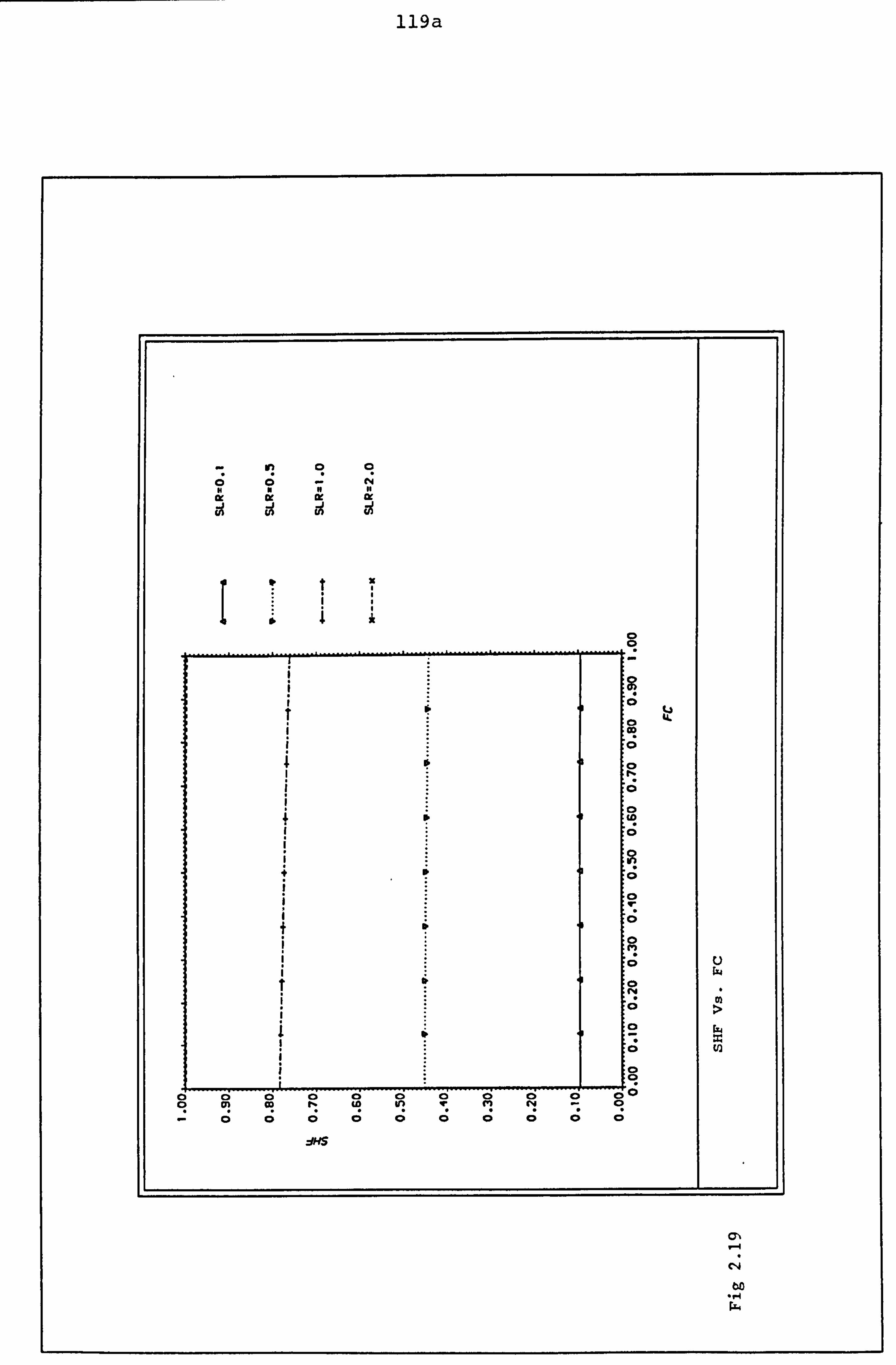
119a

C14

119b

-4 to IA

1

0. i 0 ........... 9

4J m

C; 0 U.

C! w

0 I

m 0

lu 0 0

,e 43 > $'

C; cl 0

44 0

r. 0

4 4. )

X I I I m 44 M

C; :3 0

0 >

19 --------------- a00

V! 00000 ci

Cý C'4

to . r4

119C

oc

120

Another feature of Figs. 2.28 is the fact that the difference between a simply direct gain feature B=O and a greenhouse B=1.0 at same weather conditions is a temperature difference of about (22.1 - 15.6) or 6.5 46 C.

On considering eqn. 2.13 it was mentioned that the effect of the multiplier FX (heat removal factor) is to reduce the calculated useful energy gain from what it would have been had the whole system been

. 4. ); to what it actually is at( Tp o- - 'r

using a fluid that increases in temperature as it flows through the system. Thu4 higher values of building envelop temperature from actual flow values or larger UAAVvalues should show a decrease in the multiplier VL from actual. This is seen in Figs. 2.29

9 where for higher tl% values, F it decreases.

Again, from the definition of the multiplier F$L above (heat removal factor), and as already pointed out higher conservatory sizes (B values), approaching the greenhouse (B 1)., represent higher conservatory temperatures; as the actual building envelop temperature increasing differs from conservatory temperature the multiplying factor Fp_ (heat removal factor) decreases. This is illustrated in Fig. 2.30.

Figs. 2.22 and 2.23 illust- trate the variation of the multiplying factor FA (heat removal factor); with AarjX'C+

, for various conservatory sizes. Firstly, the size of the conservatory does not considerably affect this pattern.

121

More importantly as the storage mass increases or heat transfer coefficient U*+, pfrom building envelop decreases, the heat removal factor asymtotically approaches its actual value (i. e. unity).

This is due to the fact that Uet the heat transfer coefficient from building envelop to ambient has decreased considerably and more uniform conditions in the building envelop can be more represented by a single temperature e. g. TW*

Figs 2.24 showsthat for low ventilation or infiltration rates the temperature difference for various conservatory sizes is much more marked than at higher ventilation or infiltration rates. Also for any given ventilation or infiltration rate, the conservatory temperature asymtotically reaches ca for no ventilation or infiltration- Wiwi ; -AX = 0.0. Also, for any given ventilation or infiltration rate larger conservatories generally represent higher temperatures.

Figs. 2.25 again illustrateithe fact that the multiplier FjL decreases as conservatory temperature Ta, increases for any conservatory size. At T L. 0 =_ TIjL' = 11 .60aC, the heat removal factor iS unity as should be expec: U-4 from the definition of F,,

Larger conservatories (B - values) illustrate a more marked variation in Fp. versus T,.,, . This is because the actual difference in building envelop temperature from conservatory temperature is much more pronounced with the introduction of larger conservatory.

122

Figs. 2.26 illustrate that the equivalent heat transfer coefficient from building envelop to ambient., LR40+, increases with increasing conservatory size w. r. t building (B - value).

Figs. 2.30 shows that the heat removal factor or multiplier FA decreases for larger conservatories as should be expected (from a simple d. g. B=0, to a greenhouse B= 1).

Figs 2.31 illustrate that the Tt. decreases with increasing infiltration rates into conservatory at all insolation levels considered.

Figs 2.32 and 2.33 illustrate the frequency of occurrence of SLR values ver

' sus specific

SLR values using Typical Reference Year (TRY) hourly data for Milton Keynes U. K. Lat (52.8N) (Linford passive solar houses); and Kew, London (10 yrs reference).

A 5th Degree polynomial proved sufficiently accurate to represent both models; with a multiple correlation coefficient of R- and R=0.98 respectively. The results thus validate the approach of Cowing and Kreider (20) validating them for U. K. locations.

122a

C14 C-4

Cý 44

122b

rn

f. u

122c

P. C; C;

000 If 0 81 It CD in m

t

. ........... - ----- C: V

C; cc, C; 0

0 4)

w 0

: 3 0 0

Art 44

0

C; E-4

w 0

9

- . 0, -1 0 r. OD V.

1 CD

U 1 00 w C4 1; ! w;

9; T dwai *Add5W0,7

Cý

04

bo ., 4

122d

c; C;

0000 11 it to ca 4m cc CD co co

I -* . 0, ,.

A 11 . co

3. w

." .0 1 .

'A

lo, 0

, 01 ., 1 -1 01'

0 0 00,

.. ", "'0 .,

0. - q: t7l

I ;,,, f ,. 10

in 44

a ci c;

! 2w IMP In in on C;

x- d-4 -IDDJ 7p-w

L

Lr, 04

Cý

60 ., 4 rX4

122e

0

> 00 w w > > 0 9) U

Öl c:

0 0

10 ýi

w _H

H tu :i

A 44 0

c; 0

44 -H 44 ;1 44

0 0 0 w

44

fe 0 w w

(0 -ri

0 -0 9

r. a)

H 0 >

> H >

-0 , C!

v. Co N tli

19 r! li cs Ir cil 14 CD 00

N9g! r: v! lq; 01 cn

94 (4 9

94 In (n CD Co CD Co t4 c4 c4 c4 (4 t4

ban

%D

1

44

122f

C4

0

in

0 w 4

44

0

0 co it to 41

to li

V) r.

r. 4)

% ,4 ., 1

1 co I 0

44 V

04

E-4 44

. 0

0. 0

on 0)

r

r. 0

> C:

6 lqý tq

6Nw0 co N ca 0N

9 V! U! 1,: 9 ri Pý 0 0 1" CID CD fý r- ww C-4 C4

T

Cý

N

122g

$A

je 40

vi

>

a cr4

,A O'A CA ... to -0 41 !i %ft as

>... 4

# 43

LwV, 4

:ý6 :)P. - a 4)

m

8 m 0

CD C;

li 0 0 $4 0

44

0 ,a

4J m 0

0

0) *0 m r

r-4 ýA

0 u

:5 .0

co N0

0 0 In 00 co r- r- T To !2

00 Cý

C14

44

122h

ej ok ic

0 -1 i: 4)

--- ------- - $4 0

44

44 44

La a) 0

w 44 41

w 4. ) 0 0 41

44

m > (a 0 4)

0 $4

44 4) 0 .9 4. ) 0 0

44 4) 0

9 V! Ci ri 9 Pý 00 m m ol co

N N N N

ban

C14

bc

1221

0 w V!

as

41 to 0)

. . * - --- - ..... ......... ------------ ... I

w ; C 0

9 0 >

W 0

C; rq 0 41

2 w 44 to r.

C; H -4

44 >1 0A

4. ) ýg 00 0) H

44 44 C; 44 -

0 41 u

44 C;

0 9

9 ci ci ci Ci ci C; V! C, m rq ;m m r) cl)

cn

14

rx.

122j

A 0 > in a 1 7 a

3. >

in In is -0 11 0> In tri 0

00 CD

0

44 4) >

6 44 0

4. ) to

C: 0 0

0 4. )

40, S,., -,. * N

C; 44 0

-W it w xw it

>

. *a. x4t 4) IV >1

4. ) w m 0

It 4. ) m c OD ý)4 0

w 0 0 . lj 4)

is 4) 0 rZ

U) C:

41 0

0 -H

0) 41 A 0

w

V! _ Iri rý; C" - ri vi rý tri

0 LO li Cý Pý r! C, r-

0 ;. -, F; Fi a0 al CD 0; C; 'm

Mm .4 C4 (4 C14 C4 r: C4

cn

Cý P.

122k

en 't Lf) 't tý

ýzt r- %0 C14 It bn r- 00 kD ON ON Ln P4 -4 00 't 00 - 't ý4 cli 10 (D ID C) Lr) U) rý Le-I -- C) 'T 00 -0" 1ý0 - 60 r- -4 Ln Ln -4 en

fl- Lr) -0 -4 C-4 I C-)

+

ýX4

ho (1) w cli

%D + -4

rý

M

j in

OL 11 0 u

tio u

Ir 0

+ >

14 0

r4 CD

C; z

1-4 OD

44 V) 0

C; C: 0

0) C:

q >I

-4

rz 0 C: 0 co 44 0 r. 41 PIN ; 1-1

ý4 C 4 0

P.

.......... U) ..... ............. ....

10

to w ........................ :3 Q) w --- ------- --- -- -- - 0w - -1 0

.0 0 oll; Q! V! 9 Lý C!

.C =1 ; V- rs vn m C4 0a

4-1 Ln Q (&7S)d W.

0 44

cn w

C14 >4

C14

0 -1

1221

r- Lr) rý ON

in rý C4 , CN

V) I C)

4!, 11 + 94 ý4 cn

to

94

co

0

0

$4 bo 41)

Ln

z

rn 41 4-4 C)

-x

%o C*4 cn 00 00 cr, in r-i 'm 't rý a% Ln rý C'4

aý 00 r- cl) 0 cl) 00 C> co 00 00 . C> I,, 1ý0 - Cr% Ln

-T Ln "o r, -t C-4 Lr) q C'j

If It if

w VA

4

123

It was then useful to apply both the analytical techniques employing a parabolic p-SLR and polynomial p-SLR, detailed in sections I and 2 of this paper, to actual monitored building and weather data.

Data available for the Passive Solar Heated Linford Houses in Milton Keynes for the Heating Season May 82-April 83 was used and the SHF, SLR distribution for 3 houses (33,35 and 36) obtained.

Both approaches were applied to each of the 3 individual houses for different load ratios (EdIL-) and all 3 houses together using both methods. The SHF, SLR distribution for 3 daytime to total load ratios for Houses 33,35 and 36 are presented in Figs. (2.34) (2.36) and (2.38) respectively using method 1.

For the house load ratios considered the weather data showed that both houses 35 and 36 yielded higher SLR's compared to House 33.

The plot for all 3 houses and loads appears in Fig 2.41, using method 1- the Gordon and Zarmi Approach. The lower regions for SHF or SLR can be seen to be those for House 33, while houses 35 and 36 characterise the higher regions of the plot. A key result is the fact that the actual monitored data (hence SLR) fits the theoretical results using Gordon and Zarmi's approach (parabolic p-SLR); to the Linford House data.

These theoretical results for a direct gain Solar Heated reference house have been presented in Fig 2.11. It can be seen that the patterns are similar, though the actual observed SLR range vary, as these are climatic dependent.

124

Hence one could say that the approach of Gordon and Zarmi could be effectively used in monitoring the performance of actual systems.

As information was available for the auxilliary number of Kwh's employed in heating room air for each of the 3 houses (Period Oct. 82-April 83) heating season; Gordon and Zarmi's approach has been used in determining the auxilliary energy consumption of each house per month from SLR and SHF weather data. The auxilliary energy consumption (QAUXCGZ) for space heating as computed by Gordon and Zarmi's method in Kwh's is shown plotted against the actual measured auxilliary energy consumption (QAUXM) for each of Houses 33,35 and 36 in Figs 2.35 2.37 and 2.39 respectively. The three plots show that House 33 with lower SHFIs auxilliary heating energy consumption per month is generally higher than Houses 35 and 36 with higher SHFIs, as should be expected.

The near symmetry of the three plots is an indication of the fact that the analytical techniques of Gordon and Zarmi predict the auxilliary space heating energy' with a reasonable level of accuracy.

(See the plot for all 3 houses, Fig 2.40), The model appears to over-estimate auxilliary energy requirements. This region in plot (2.40) is relatively small. * For almost all of the data sets the model accurately predicts the auxilliary energy requirements. Also it must be noted that_ the load ratios employed in these computations (L/Ld) were hypothetical values as opposed to the actual values. It could be pointed out that it seems safe that the model rather than under-estimate auxilliary energy requirements in the heating season (Oct. -April), does marginally over-estimate it at periods when least auxilliary energy is needed, and again marginally under-estimates it during periods of highest needs. The later is certainly a drawback. Cowing and Kreider (20) suggested that the deviation of the estimates could result from the fact that the model assumes the insclation impinging upon a vertical south facing surface varies sinusoidally during a clear day, with a similar ambient temperature profile. The effect they suggest Is to match instantaneous solar heating energy with space heating loads in a less favourable manner, than is assumed in-the model. The authors in (1) and (14) also demonstrated analytically that in houses

125

with relatively low relaxation time (- five hours) auxilliary energy requirements are under-estimated by 6.4% Cowing and Kreider (20) further suggest a possibility of random nature error in the input measurements. All sources of input measurement errors must be eliminated or at least quantified. They sum up by suggesting estimates of instananeous and contin- uous measure

- ments will permit an estimation of the uncertainties in average daily auxilliary space heating requirements for all months and or locations considered.

The main difference in the approach of Cowing and Kreider (20) from that originally pioneered by Gordon and Zarmi (1) is in the fact that the later employs a parabolic distribution function for P(SLR), the frequency of occurrence of computed SLR values. The former, however (20), employs the actual frequency distribution from typical meterological years data; a 5th order polynomial in the case of Milton Keynes. It should be expected therefore that as recommended by Gordon and Zarmi (1), Cowing and Kreider's approach yield more agreeable results. This appears to be the case comparing the computed and measured auxilliary energy requirements by both methods for all 3 houses i. e. Figs 2.40 and 2.48, about the line of symmetry. The data sets lie more evenly around the line of symmetry in the model using actual p(SLR) distributions Fig 2.48. If we now consider specific auxilliary energies of 770 Kwh/month for example, it can be seen that the two models agree exactly for House 35, fig 2.48, as opposed to Fig 2.40. The difference is however marginal.

The (real) SHF vs SLR distributions and measured vs computed auxilliary space heating requirements per month for each of House 33,35 and 36 using the 5th degree polynomial from weather data, for Linford Houses, for p(SLR) is shown in Figs 2.42 to 2.47.

126

From Figs 2.43,2.45 and 2.47 deductions can be made on the effect of the load ratio (L 11: A) on the computed auxilliary energy, for each individual house; the absissa axis. it was assumed in plotting the curves that the measured auxilliary energy at each of these load ratios is non-variant; (the ordinate axis) as monitored data for various load ratios was unavailable. This also certainly affects the symmetry of the curves. If one considers the computed auxilliary energy requirement_(abiLissa) for House 33, Fig (2.43), load ratios of (LA /L )-0.3 and 0.25 yield almost similar auxilliary energies. However, higher day load ratios (LAIL 0.5 yield higher auxilliary energies.

Physically, this means months with higher average daily loads require higher auxilliary heating, as should be expected, for the solar inputs should be low for days with high loads. Figs 2.45 and 2.47 on the other hand for Houses 35 and 36 shows that the auxilliary energy (absissa axis) _.

Aecreases with increasing daytime load ratio i. e. ( Ldd /Z) increasing. This may be explained by the fact that days with low daytime loads, represent days with high solar inputs, but less auxilliary needs in' storage from daytime for use at night time, requiring more auxilliary heating, at night time.

On the other hand, for days with high daytime loads, the auxilliary inputs during daytime for use at night time when much heating is required is higher although solar input during daytime is low, resulting in less auxilliary needs at night. The effectiveness of storage and solar inputs into the thermal mass therefore plays a role in auxilliary energy requirements.

A balance is made here between the solar inputs to storage and the auxilliary heat input to storage used up at night time, which is itself an indication of building performance. Residual energy from daytime used during night time comes into play.

It appears that the auxilliary energy needs for each of the three test cell houses favour House 35 over House 36, in turn over House 33. See the range of the absissa axis of figs 2.45,2.47 and 2.43.

126a

. 19h

.. p 11 04

04 0

N 11

m 1

V. it

>1 m

V -1

13 j

1) j

-3 j

t z

z 0 E-4

i. %

CL 0)

ký*-.. % % ,,.. .

0 10 4. Q dc % .. %%

0N

1

0 10 ci ci 0 00 9

0000 li ri Cý 1%

a 9 too

Ln rl m N

dus 42 04 or..

126b

0 r4 r) e 91 0U 0) oý

al to 0 10

Ln 0 10

; 4. 41 w 0

u

IN t 01 >

w 4) 0 w

4' :i

01

ob b = . dp

DU 1 Co 0 ci 0 r,

ö00 to

0000 0

r4 g

LD -

126d

04 T, '

00

av 1) iJ

x 1ý 0 J 0 U)

>1

Jj

0 u -11

............ - ---- --- N ý4 1

x :)0

ci 2 go m V; > co

0 4) 0 r

.4 +# mw 4) 0 Z 44

10,

$ 4 0

-4 co ý4

C-4

r t; m -H

lu

00a0a 60 to C4 r. w Cl) N

c"x., janve

126e

Itr I Nm to 0

q, N

14

a] 4)

0 to

w (d 0 u

---------------- r: EO 0 0-

> fo -4 N

% 0 at %% to 10

(I A

in 04 V w

r. 0 0

44 C:

10 ý4 0

0 . 44 0

611, 0

04 m 0) ý

-------- ------ 0!

0 0,0 0 ao

44

fn C14 in ir wC

126f

0 .H 41

cq q.

13 1) -i le j 0

u

w

>4 u $4 fu

u

10

4

0

r- ol

4 -1 4

R 's . m. 0

lb u 0)

tý 0 10 0) V

In 4 0

0 in

0 0 Ln 9n in In 9

E V2za M r, w Ir

126g

0

4)

A9

w ww

>1 tt

0

4)

b

0 0 m

4 M &I Z lob > 0

+

+

01+ 0 0

0 q4

0 (P)

+ go z A

d) w 4 A 0

p b 4. 1% E-4 44

lb N c

ci ci ci 0 0 0 w

0 Ch 0 0

0, rf (QAX) janvo

12bk

>1 4)

N m

0

i j

t

ol 0

- ----- ---- w

0 R

0x lk

0 44

.4

to 0

w w Lf)

in m W :3 0) 0 M

V 4)

C4 w

In m >

m : 01 8 (A L)

1: 1-0 r

0

ci cs 0 0 N 0 co w in in in in V)

MRS

126o

.t

: w M 0, W n.

ei ri

99 w b4

0) w ww

x xx (0 ..

V to

0

---- ---------- -

a 7 r- v v

0 01 0 u 4)

> 0 x Cb

op w w

e 4 :1

01 0

41

4 0

ci 00 0 0 0

rý 0

Co 91 rý in A4 94

126p

(Y)

.j j j % % % -j J J U) m in to m M M

EO

1! t -A 0)

(o 0 of =

w w 0 0) 44

... q

4 0

0.1- p 0%

E-4 0

NOW 11. m 44

Pa. 14 0 0

to w ol > 8

## + W 0)

ca E-4

.64 14 VP

'o 8 (14

,0 ci ci 00C; 6 co 4=1 0 I,: G! ri Iq 9 1: C! vi li w in v Ir q. M 94 N

127

SECTION 5

CONCLUSIONS AND SUGGESTIONS FOR FURTHER WORK

128

A simple analytic method for calculating the monthly and seasonal thermal performance of passively-heated solar ho'uses has been presented in closed form.

Both the formalism for a direct gain house with and without an attached conservatory have been presented.

Furthermore, typical reference year meteorological data for the Linford Passive solar houses, Milton Keynes and Kew Gardens, London (10 years hourly ref), are used in determining the actual SLR-distribution functions for both locations.

The methods employed for the formalism for the attached conservatory have been developed from first principles in the study. The results are compared with the simple direct gain cases also considered. Some apparent results occur.

Firstly, it should be mentioned that the main advantage of the analytic technique is that it provides a useful tool.. for easy calculation., of the dependence, of thermal performance, on buildings and climatic factors. Detailed study of factors 04 conservatory size, ventilation rate into the building, and so on, have been under- taken. The conservatory temperature TQ, heat removal factor. of building envelop, F& , and ventilation and infiltration flow rates into the buildinghave been

studied.

129

The conclusions from the discussions in Section 4 show fundamentally that the introduction of the conservatory to the same ref. building (the simple direct gain house), introduces higher SHF values.

From Figs. 2.28, it was con- cluded that for conservatory temperatures above ambient, the conservatory temperature increases with the conservatory size B with respect to the building.

From Figs 2.28 it was depicted that the difference in temperature between a simple direct gain feature B=0, and . greenhouse B-1.0, at same weather conditions is about 6.50C.

It was demonstrated from this study, see Figs 2.24, that for low ventilation or infiltration rates, the temperature difference for various conservatory sizes is much more marked than at higher ventilation or infiltration rates. Also, for any given ventilation or infiltration rates, larger conservatories generally represent higher temperatures.

The heat removal factor Fp- decreases in increasing conservatory temperature Te4, At Tc,, - To_ , FA becomes unity. See Fig. 2.25.

Figs 2.31 illustrates the fact that the conservatory temperature decreases with increasing infiltration rates into the conservatory.

Using typical years reference data for 1) the Linford passsive-solar houses, Milton Keynes and 2) Kew Gardens, London (10 yr hourly base ref. ) solar to load ratio - SLR - values; Were computed for both locations, and the frequency of occurrence of each SLR value determined from the meteorological and building data, i. e R(SLR). The p- distributions for both locations is shown in Figs. 2.32 and 2.33.

130

A 5th Degree polynomial was then fitted on both curves and the coefficients representing the P- distributions determined. A correlation order of 0.97 and 0.93 represented a good fit, as in the work by Kreider and Cowing (20), thus validating the approach to two U. K. locations.

A further extension of this work will involve the compilation of data for about 40 houses and estimating the daily auxilliary energy from this approach; then, comparing with measured data as in ref. (20),

'The case of an attached solarium can also be considered.

131

As an indication of the practicability and validation of the analytical techniques details described in this paper, the case of 3 real direct gain houses was considered. The houses are of the direct gain type and are described as Houses 33,35 and 36. They are the Linford Houses in the Milton Keynes District in England. Meteorological data and records of the auxilliary space heating energy usage over the heating season (Oct. 82-April 83,7 months) has been compared to computations by each of two methods.

The analysis is carried out for these three houses independently and collectively using the two methods. Method (A) assumes a parabolic distribution function for SLR, p(SLR), given by eqn. (1.3.1), sufficiently describes the frequency of occurrence of computed SLR values, over the heating seasons 7 months' duration. Method (B) uses the real statistically determined frequency distribution p(SLR) from the weather data. A 5th order polynomial sufficiently described all p(SLR) values with good correlation (r - 0.97), Fig 2.32.

The average predictions of auxilliary energy usage in (Kwh/month) by model (B) using actual p-SLR weather data appears to favour observed records more than Model (A) using a parabolic p-SLR, as recommended by Gordon and Zarmifl2o

As many houses in the U. K. use conservatories to further enhance building performance the rigorous equations derived in this report for such situations will obviously be of immense use in designing buildings in the U. K and Europe at large. Finally, it is hoped that the ana-lytical results presented will help understand the physics of the study.

132

CHAPTER 6

REFERENCES

133

IDVVVIDV? Jrvc

JM Gordon "Analytic Model for Passively- Y Zarmi heated Solar Houses - 1. Theory"

Solar Energy, Vol. 27, No. 4, pg. 331-3 42,1981.

2. JM Gordon "Analytical Model for Passively- Y Zarmi heated Solar Houses.

2. Users Guide. "

Solar Energy, Vol. 27, No. 4 pg 343-47 1981.

3. W. O. Wray "A semi-empirical Method for J. D. Balcomb Estimating the Performance of

R. D. McFarland Direct Gain Passive Heated Buildings"

Los Alamos Scientific Laboratory Publications LA-UR-79-117(1979)

4. W. D. Wray "Trombe Wall Vs Direct Gain: A J. D. Balcomb Comparative Analysis of Passive

Heating Systems"

Los Alamos Scientific Laboratory Publication LA-UR-79-116(1979)

5. J. D. Balcomb "A Simple Empirical Method for R. D. McFarland Estimating the Performance of a

Passive Solar Heated Building of the Thermal Storage Wall Type"

Los Alamos Scientific Laboratory Publication LA-UR-78-1159 (1978)

134

6. R. D. McFarland "The Effect of Design Parameter J. D. Balcomb Changes on the Performance of

Thermal Storage Wall Passive Systems"

7. J. E. Perry Jnr

R. W. Jones

9. N. E. Neba-Fabs

10. P BCrdahl D Grether D Martin M Wahling

0 11. S Schweittzer


"Mathematical Modelling of the Performance of Passive Solar Heating Systems"


"Private Communication Zarmi, Jones"

Los Alamos Scientific Laboratory (Oct. 1980)

"Solar Energy Modelling and Collection by Direct Gain Rooms"

MPhil Dissertation, Cranfield Institute of Technology, SME 1988.

"California Solar Data Manual"

Lawrence Berkeley Laboratory (1978)

"A representative 'Average' Weather Year for Israel's Coastal Plain"

Report No. 3-78. Agricultural Research Organisation, Bet-Dagan, Israel (1978)

135

12. B. Y. H. Lim "The Interrelationship and R. C. Jordan Characteristic Distribution of

Direct, Diffuse and Total Solar Radiation"

Solar Energy 4(3), 1 (1960).

13. H Tabor "Radiation Convection and Conduction Coefficients in Solar Collectors"

Bull. Res. Council Israel 6(C) 155 (1958).

14. J. M. Gordon "Massive Storage Walls as Y Zarmi Passive Solar Heating Elements:

An Analytic Model"

Solar Energy Vol. 27, No. 4. pg 349-55 (1981).

15. D. M. Utzinger "The Effect of Air Flow Rate J. W. Mitchell in Collector-storage walls"

Proc. Am. Section ISES Conf. pg. 831, Phoenix, Arizona

(June 1980).

16. M. W. Liddament "Aspects of Natural Ventilation in Passively Heated Buildings"

Conf. Proceedings: The Efficient Use of Energy in Buildings. 2nd U. K. ISES Conference, C46, Sept 17,1986, Cranfield Institute of Technology, Bedford, England.

136

17. ASHRAE(1977) "American Society of Heating, Refrigeration and Air-Condit- ioning Engineering Handbook"

Published - ASHRAE (1977).

18. R. T. Larsen "Digital Simulation of Energy Consumption in Residential Buildings"

Proc, International Council for Building research studies and Documentation (CIB), British Building Research Establishment. Published: The Construction Press Ltd, in conjunction with CIB (1976).

19. W. C. Randall "Predetermining Aeration of E. W. Conover Industrial Buildings"

ASHVE Transactions, Vol. 37 (1931) P-605.

20. T. Cowing "Solar-Load-Ratio Statistics J. F. Kreider for the United States and their

use for Analytical Solar Performance Predictions".

Journal of Solar Energy, Engineering Nov. (1987), Vol. log, pg 281.

21. T. W. Cowing "A New Passive Solar Space Heat System Design Method for the United States"

M. S. Thesis, Building Systems Program /Energy, Univ. of Colorado, Boulder, Co. (1984).

137

22. I. J. Hall "Generation of a Typical Meteor- R. R. Prairie ological Y, ear for 26 SOLMET H. E. Anderson Stations" E. C. Boes

Proc. 1978 Annual Meeting of AS/ISES Vol. 2.2, Denver, Co, Aug. 28-31, pp 669-71 (1978).

23. N. H. Nie "Statistical Packages for the C. H. Hall Social Sciences"

J. G. Jenkins K. Steinbrenner Mc-Graw - Hill, New York (1975).

D. H. Bent

24. W. O. WraAj "Sensitivity of direct gain J. D. Balcomb space heating performance to

fundamental parameter variations"

Solar Energy 23,421 (1979).

138

CHAPTER 7

PUBLISHED REPORTS

139

PUBLISHED REPORTS

1.

2.

3.

4.

N. E. Neba-Fabs "The Design and_Construction of a Solar Energy Collector with Corrugated Iron Sheet as Absorber for Domestic Water Heating".

B. Eng Project, June (83), Hech. Eng., Ahmad%Bello Univ. Zaria, Nigeria.

N. E. Neba-Fabs "Solar Radiation Estimates from available Meterological Data for the Republic of rAmairnnn - 11

N. E. Neba-Fabs V. A. Akinsete A. Falada

N. E. Neba-Fabs

5. N. E. Neba-Fabs B. Norton J. C. McVeigh S. D. Probert

MSc thesis, Dec. 84, Mech. Eng University of Lagos, Nigeria.

"Solar Radiation and its Estimation in Nigeria and the Cameroon"

Commonwealth Science Council, Mauritius. 1985.

"Solar Energy Modelling and Eollection by Direct Gain Rooms-

MPhil Diss., Dec. 1987, Mech. Eng., Cranfield Institute of Technology, England.

"Solar Radiation Models for týe Cameroons"

I. S. E. S. World Congress, Hamburg, Germany(jq8-7)

140

CHAPTER 8

APPENDICES

Al. Solution of Heat Balance Equation for Direct Gain House,

From eqn. (1.3.9)

(ir, C) dT 411 4t 4=''-- 'JSA ( TS T, )

S9 Ata- We denote the storage mass (MC), D

I -F)Q, zATd ana T, =C A+d S

Eqn. (1-1) becomes

Ll =A- at's -C) (A L-2)

d w.

or !U+ SV =A+ BC (A L-3 am

writing A+ BC - K,

, )I-' +SI-K =0 dx

dl +

ze e -b dl +3-I- P- v=K et d -jc 3> 1)

A zc A le !! e 3) A 1-6 3)

integrating both sides W-r-t x

1xi. u. ZC (A 1-7

Z. lb

Z-a -X

ce

a (1-F) Q, -[ USA rn Os It

+ 7ý 1 At d USA +Ca

(A 1.5)

(Al-9 )

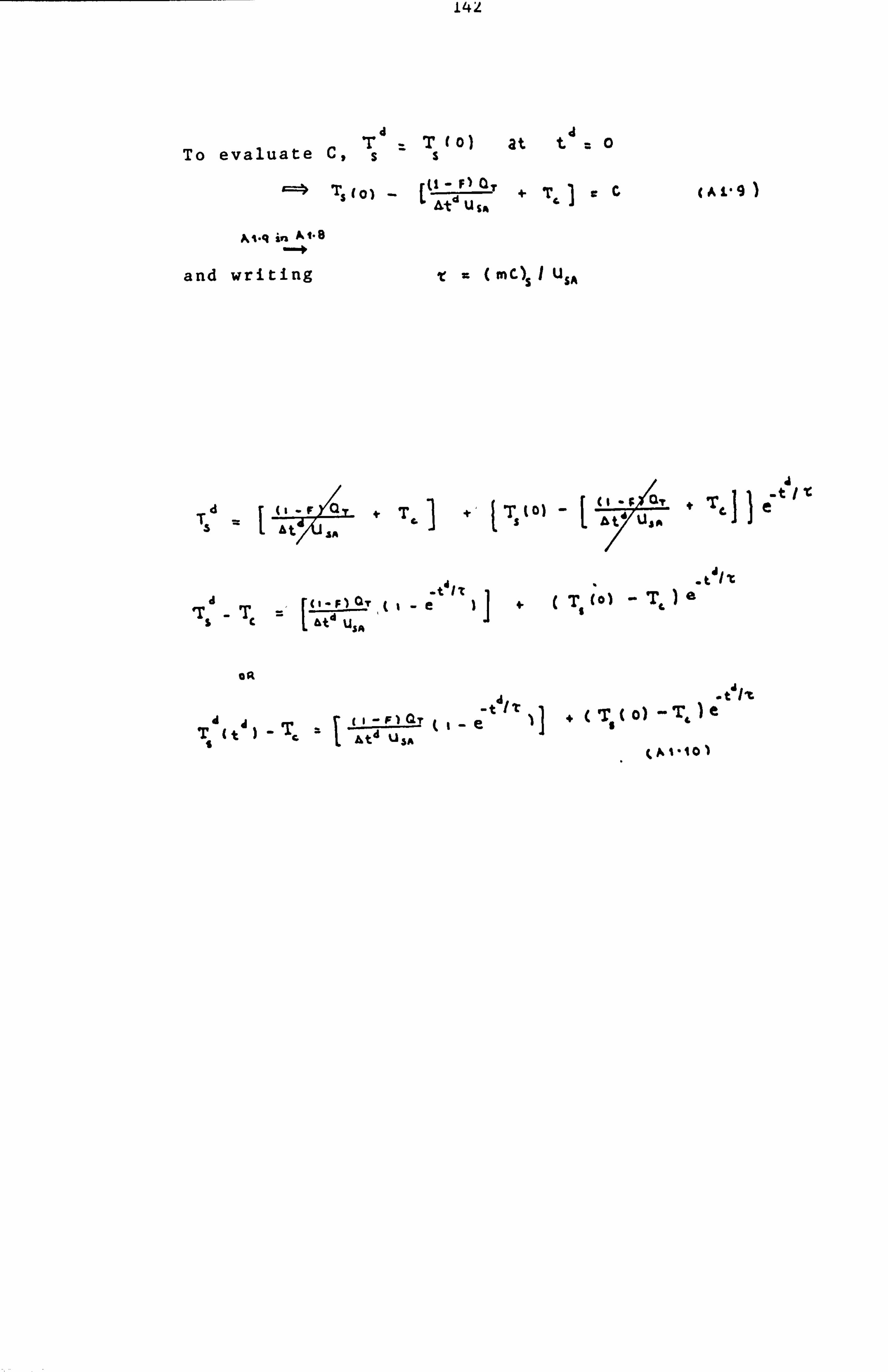
TT (0) at t0 To evaluate C, ss

Ts (0) -[ Ll -CP OT

+ T, I. C. (AL-9 ) At u sok

N, t. q

and writing MC)S 1 USA

T3 =14.

Ta -FI OT (, -;

t4 Vt ,]4. ( lý

ic1a. tli -t

Te = ,

ci

- to) -T

t

l(%-eT-T. Tcu1 s( 0)

it 4u Alt

A2 Solution of Heat Balance Equation for the WaterWalt House (Eqn. 1.5.1)

From eqn. 1.5.1

(inC) dTý d

Idt d=(.

40,1 At Ud Ssa( Tsl Ta 1- U$,, (rj - T,

We rewrite eqn. as C4 =A (4 - C) F dx

Z4J=A++bC+EF dx

1, U4 =I-r, ýCh2 -2 )

d: C

where A 642 t

Ga b+ E

From eqn. (Al. 8) the solution of (A2.2) is

D (A 1-3)

+ Usa Ae ( U. Sa 4. U, ) uj*U 3 St JA

41

-Usa + USA (A2.5) rn C)

3 A

(A2-2 )

lAsA Tc (A 1-4) 41 US& + QSA

TS=Q, + T. US . US. )l (.. C), I t4 dT at +da (U

S& 4 USA Us& +U SA (A 2-6

if T (mC), I( Usa + USA then substituting

5 sto) , at td= o in eqn (A2.6), gives, Tj =T

OL Cý T

&0( u, +u sa Sot

A-1.6

T (t U Ul.

+

Aa Usa Ta U,,, % Te

di J

ula + USA us& 4, USA

(A 2-7

'i I Usa.

\Ta

4 uu

U S& Ta.

ui+e \U

144

or

a4ajA -t aIt

Ie -t it', ) .- -t I't USX T, u,,, T, + T; to)

T (t zmý %. A - Us^

3 &td ( us& + usJ

ataA Adding

I and subtracti ng

usaTl. e USL + ýASA

an R-14-5 of Al-s 21*40

- t4 1-t 4a -t

41 It dj

ad Q-r (I-6 u" eCT, TaI T, -ld a

Ae(U, a + USA) U S&

U3A

41 .t us,, Te. Cet+T (o)e US3 TC. e usa + USI, usa u SPI

The 3rd and 4th terms added gives

T, - 7ý e

Hence eqn. (A2.9) becomes

-talld d -el-C4 41

4 4d e Us& (i -eI CT, -TA

TT 4d at + USA + USA ,( U'S us,

with given by -r C0e.

t -C

X-X-lo

A

i(U 41 +U A2.1i It ( rnc), / 5a

144a

A3. Gordon and Zarmi (14) illustrated

that the non-linear heat diffusion

through the massive storage wall can

be treated as a linear one node model,

for wall thicknesses of practical

interest.

145

EQN. A4. SOLUTION OF THE HEAT BALANCENIN DAYTIME

The daytime heat balance equation for a direct gain building with attached conservatory is

aA(I-FI USA Td LmC), dT. Idt atd

+uTdTa "O's ce I

writing

(MC) T tl 35

A-if: At

6) USA

C

=8 U0

Co r.

dI At

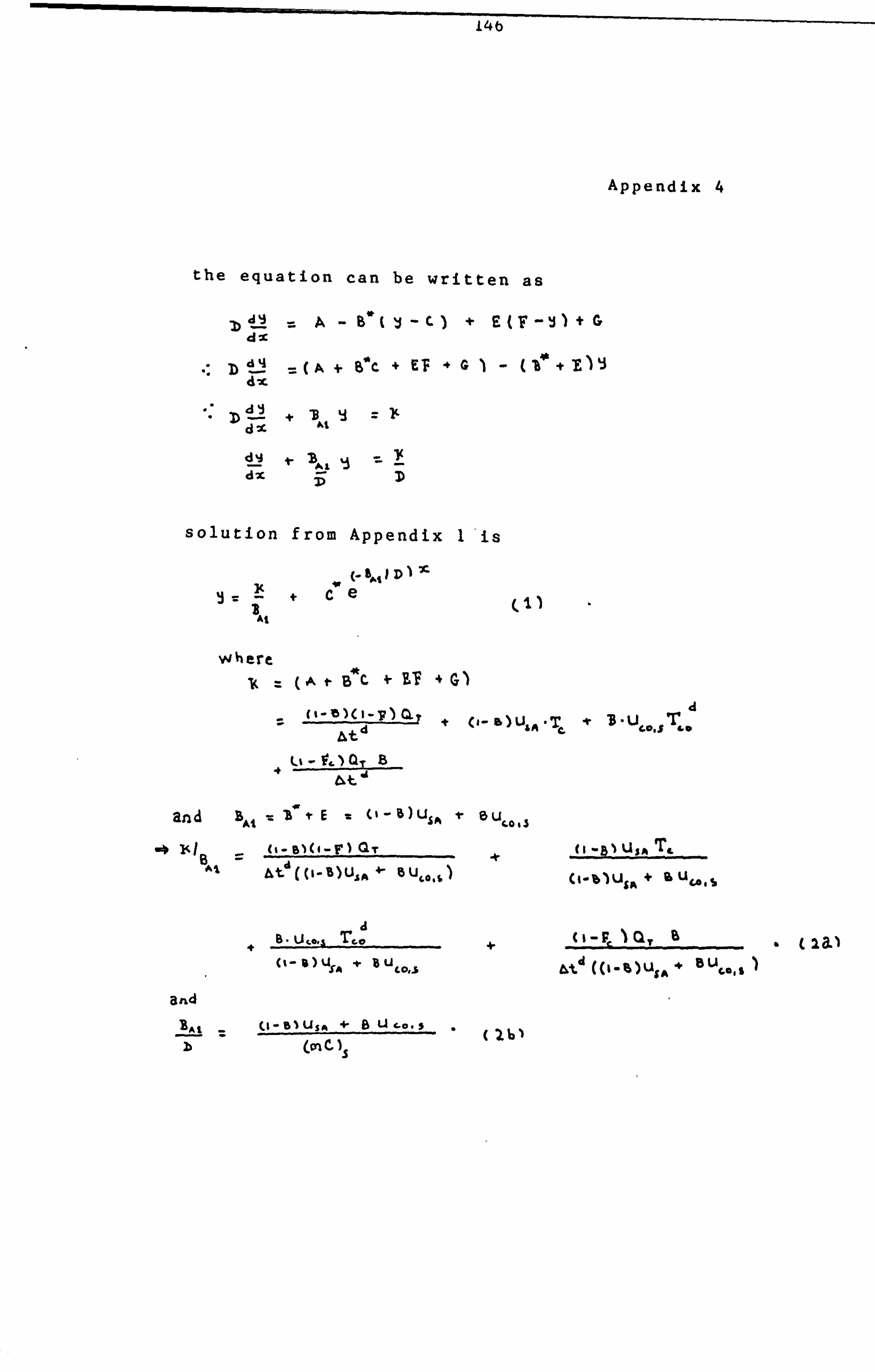
146

Appendix 4

the equation can be written as

-b L%j =A- t* (2- r- 1 dX

D '124 +E d%

-D 1L3 + ci 2c

LY B', Z dx 5

solution from Appendix l'is

it (- 5ý,, ID

ce

where 1( (A f- B*C

15 )c I-+ (1- &)U -T + S*u At d &A C,

Ll-v, )QT f3- 4t 'A

and IE -a 0 Us, v5 Uc. 0 3 (I- 5)(4-F) (IT T, Atý(cl-B)u" +- (1-1b)USA + SU

cAss

+B-u+ "SA +U

Coll

and 'RAt al USA +U

b (me) 3

(%-F 1. ý

&tl «1-1b)us, .

147

(4-3)ts-P USA TS

4 +. au, At (ii-DIU"+ lauf. U"%) (8-8)u3A �0.3

a 't u�� T,. 0. T IB

au... i U8A

IfT. (MC)t/( (1-1) UE& + BUC0.5) , substituting TSj. T (0) at t gj 0

then equation(3)becomes I

T (0) At d

uco. s T,. _

(I-S)US^ + 'hUco. s 41 in (3) d4 (1 r) OL-r

t Atd U,, +

Uc. %, s Tco (I-B)USON + S-Ulo. S

cl-b) USA Tc

(I-O)u", +

CL, a 41k

-a) USA+ 5 uce's

T'(0)

Us,, +8 U". s

8 Uco, s T,. i

(I-b)Uso, + BU&O. s

(t- a) Us#, Tc +

($-%)US, + B-UC., S ci-r. ) ar lb 1 4-

At4(to-Ous" + S'Ucels)

ci- lb) UsA Tc (I-S)USA +

Aa it

e 60

(('-B)USA

Oct -t alT of t

(s-xi(o-vl CIT o- e us* , (I- e Ts (t Usa +b uca's (I-D)USA 4, buLa. s

-tt 41

10. U.. S T. 0- a( i- e7 (1-6) USA +a U", At"((I-B)U&A + SU#. ols

T (o) e 3 0-G)USA + SU, 11,3

148

add and subtract a- UCG. TC C e- tdit d)

an FLHS

dd tdltj + U460A

e (T. -T .6 TS a U"., +

Iýt term I (use 5ubtractai T&ft ftl1rAl)

T it CL., S C

aaJej yart + terin I) term 4

-tal -C a T, to) e (S)

(term S)

Tallimg T, to LHS of ein (S) anJ conlining. ramalnins rortion

of term 3 with term 5

Tj(td Tr (1- 8)(1 -11) CL, C7 e Pt

s &tA 0 -t

IITJ ci- e

At do

-t"It cl

i uýo, s ce TC - T.. 0

4 -t (r

(T5(o) - T)e (6)

OR

Terat J anJ 2 of Gin (6 1c an be further

Comlleined t,, lif-LJ a torm in tht, Coefficient ell

It= (1-5)(1-F) + Sc I -v, )

+ -B

rL= I-T+By -Bye

This is the Solution emploje8 in k? p&nA! % (9 )I

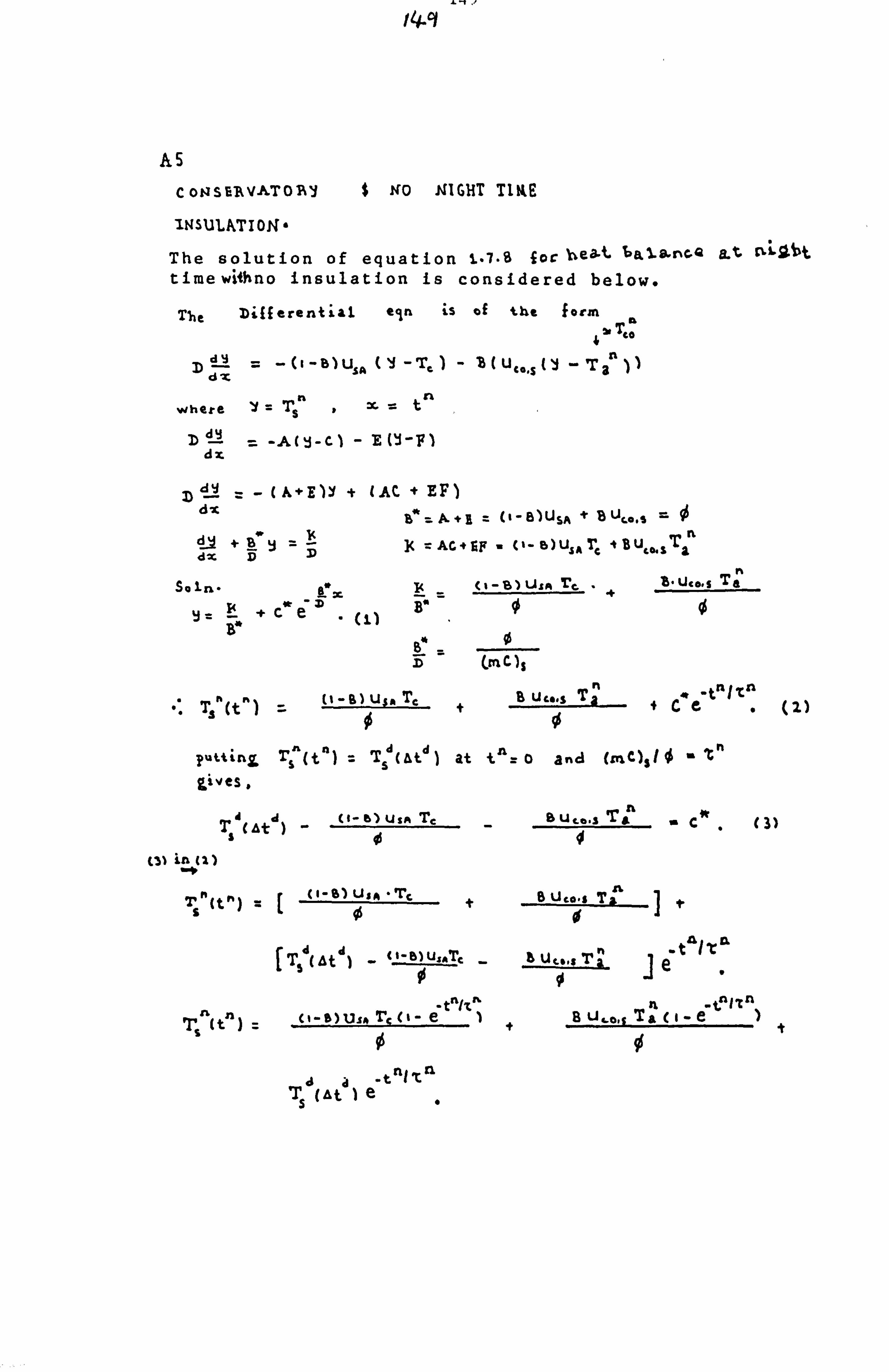
NA

AS

c oosElkvATORI $ NO MIGHT TIKE

'INSUL&TION-

The solution of equation 1-7-8 joc hea-t '6a, 1ar%c. Q jLt CLLSOýt

timewithno insulation is considered below.

Tile Zifferential tin is of the f orin T.:

4 1-2 0- B) Us, I-T. 'B ( Uc.,

s (J -T 2" d, x

Where Ts n

D L4 -A(ý-C) dx

3)42 (A+ E)Y + AC + EF d -4 i* +I=0- B) USA +B U11-S

-t su,,, T dý+ J( =AC*SF - (1-5)UArl 4% 1) 3)

h0z. tjc,, § Tan

B + c' e

(MC)s n

nn 9) USA TC B uc,,. s Ta . 01 TS (t

004Ce (2)

ddn puttinjL Ts (tg) Ts (at at tA= o and (mt)sl

b) USA TC auT C* (3) 45 4

C31 la cI )

n (t n) (1-6) UsA -Tc t6 Uco-s 'fr s gs $

tAl -C 91 b U. Lo. s Ta

T Ts (t c s) us. % Irc oeIB

Ts a (, & ta1e _tnlr a0

-thitt, and SuLtract U T, - ci- e-I t. RH5

0

Ira e-

t4. )(T, T&

(Subtracteci part I torin2)

et L%Ic

aJded lart and term

T, (At )e

Talcing T, to LHS of eln (4) 2rld cc-6101t1l.

remaining. jortion. of term 2 with terrn3 a 4 Irle

t jr, T ri

Ta

(TI d( &t

41

where

It n= Crnc)s /0 and 45 = (1-B)USA -t Buco's

151

zIRECT GAIN - EQ9 (AI*10)

Appendix 6

To obtain the energy collected by room air during Jaytime, the integral below is

evaluated as

d At d

-F Q, u (t at

at d-

tý IIc cL YQ +U

$A u3p, At cs

At d

-t d

't

u( Ts (0) Te at SA

-C cl . ell td

at

7 TJ 1. a

F('T &td

T, (O) C",

t

(2)

(1-F) QT htdic

+uT, Tr. )e- at F QT + SA T

IQ' (o+T) -+ usp, ( TS(o) - Te )-Tj- (3)

at d IT

- at i It

IT e-UT2 (0) - T, ), c e = X-F.

td SA

I- Ic USA ( TS(o) - T, )]. (4)

(1) -[ -7 -e Qa ; -- OLT T Lt Id

'&t -at

u54 ( Ts ( 0) T, ctt-e

152

MI RECT Gkl 14 Appendix 7

To c bt &in the energy Collected Ll

roorn air Juring, night time, the into. 1, ra. 1

J, elow iS CVal%lated as .

(1) =

AtA z T,

nu SA ( T, .)-, tr.

At oT (i-e je- t ryr dt, ft + VSA

&td

Atd +-ILI cn U, SA [(T 0 ]e dt

05 -t ni Ic Atim

I. -N 0, CI-eI P- I. 4- &t4

- .

)e usm (T. (o) - T,

At aT o-e). -, c ef -]+ jsp, ((Ta (0) T, ) e7 Ic. e atd

I-

d At4l I+u., v

Atd

CIL' z -c (, -e

"t e-

at d

-At a kc _At, /T

T, )e

153

AB : DIRECT GAIN Appendix 8

The solution for the average useful daytime (night time) energy gain Qj (Q,, ), i. e. solution of the two simultaneous equations (1.3.17) and (1.3.18); eliminating the second terms respectively and writing for Qn, (Q, - Qa ). Hence,

&t d/. c

ht

Od Qr c--v)-rct- e T. t. ) -T. )t '41 -e

ar (1-1r)tc I- e- At

d /-c At"/, c Q'r od

Atd +

Henceforth (I - IEý At

a IT

) ar% (I CI At IT

2. nJ art d

A+J/T 0, = 0,11 -I -i -u (1 (0) - i. ) -'r "j0 (31 At'd

t TIrl Ixi At 4 I-C 6.1 + [El. 3 . o"I gives. #

. at'/. t . 7) -C 4- at di

4. Od Od Q'r 1 Od - In ld (% -F) 'c l-d ] t43 ät, ä

OR

at /T ), r

., Ij on

4a I

Atd

[; 'Lon 04 OCL I

( S)

cat'n siJes of ein (5) 1), eft of A-erm 4

e Od (I. V)T & On d btd &td (& 4-A) n tt%

x _L A kt VIC

QT A /t

&td 53ýý PC

Qr I- F' )T id, gS,

at' (i- e"ht'

0.1-3)

154

A9 I)IRECT GAIN Jl, -Nb CONSERVATC)P-'Y:

litrt 0= (1- 6) USA + T4 U,, Oj S

Appendix 9

To obtain the energy collected by room air during daytime for the direct gain system with attached conservatory, the integral below is evaluated as

The saln for TS d Lt d Tr is frora ein CN4.7)

C1) At

da

d us,, ( T, a ( ti) T, at C1 d/, td at t

Q-r -)I Cit AtO

at I-Ca

, Usa ji-eT. T,.

PC lu SA T, 0) - T. dt

d -qar (t at

= FQT + U3A t

Ai 01/.

td 10

-

a- UCG. S t Ctdlpt a

T, Ci U. S. +

U (TS(O) - T,

USArtQLr e- At

e- T

PQ *: 1-1 Td Up, (T,. T'

r Atd 0 '4b IF

UsA ( T. c o) - Tc )E USAIQr ( 0+ Td )- USA& U,., S(Q4-C')(T'. T, ý)

d

- USA T% Te J

155

It? a aJi ng term I' ana 2 of

-t cd U. SA use Or T e. QT

is

UzU I-C d L us'kB uco's &td (Tc-Tc.

tU rl 0r -C USA( T, (o) - T, )Tdih I- &t ld 4

uuT, +u $A (T. (0) - 'r,

to mbini ag. kerins ( 1.. 2.6 ) ana terms C5 ar-a 8) rasrectivall of ein (1)

a (I)

= Tor + UsA rL G-r d(I-i. ht dIId

d0 Ata

Us, (TS (0) - T, )ta(I-e)-L, - (4)

where L, is a caln6ination Of terms 3, L, aria 7 of cin

L USA B UIC. S Ic e ht d IT d

-T d

cc

(5)

L. sepresents the contri but io n5 of the conserva-Lory ir' heating roorn air

(u)

USA rl (t- e 70 ad-133+

LIS. T, ) -C cl (IeT

156

Appendix 10

A10 DIRECT GAIN $ CONSERVATORY (Night-time Insulation)

To evaluate the energy collected by room air at night time for the direct gain system employing night time insulation, with an attached conservatory, the integral below is evaluated as 4ollows

-at d I't d

where dan. 3 (ta

Rere ' heat transfer at 11ithttitne frorn Staragt is only to room air. The Gain for (Tr'(j) -T. ) was ýLi. 4em in eqn 1-7-11

I-low ,a (1) A is given 16-y

(1) &t

n I u.,,, ( T. T, dt

0 at dt rX

d Cit Mt

us. d at

At d/Ir dt rl /'t n j U'. [ (T, (o) - T, ) eIe dt -

a n at ý

USA Uca. s ý6d__( Tý e dt

0

LISA Or ý5d 71 e+ Atc' 0--I /-C-

Id Pt dt

U5A TS (0) - T4 )': ý At 3e ]a

- _O'E"

U S84 ýB U _46d

C T. at

0. -L /T n

10

�/ a -at'/t n

r.. ýi u3A Or ed e UsA Tg (o ätd ý1

d- at'/'r d ujj% B uco. r neT, - T... 1 UCA Qlr TIIÄ od

u4. l( Tl(-I \)-

7� ) e7 A Ir . ýc91 1- -USA

B u', ', tr, Q$, d t T, - T, ,)1. (4)

157

co chb in i rq, s irai lar terms jr% ecin- Iii'-IJS

(1). a 4ý d &% -&t

ditd rL

Q= rL 0, us,, a C5 M+ Lýý'O(T, (O)-T, )"- OrL A At d0

where

L USA B UCO-S J dr, ( T,

-

ts)

(6)

or

(1) rl d rL

in Q., FU SA 't ol 95 a

n Atd 0

. &t a%a-

+ 3A

. rL (TS(O) - Tr. ) 0.0mI

where

jr, = rl 1F( %)

and 4= (I-S)US,

158

Appendix 11

A 11 11PLECT GAIN AND C-014S'ERVATORY ( No nijht insulation)

To evaluate the energy collected by room air at night time for the direct gain system employing NO night time insulation, with attached conservatory, the eqn. (1.7.14) is substituted in (1.7.16) and the integral evaluated as follows,

where 'Ca andCn are given by eqn. (1.7.4) and (1.7.13) respectively. The energy will be distinguished by an asterisk (*)

, trL

CIN) IAT, M TS

at d OT Od rL e U.

atd

a0 ata I L(T.

'(0) -T, )e- Ie dt SL -

e-tolt" rx A, tr, d", ( T, - U4.

0

Uco- T, 'u

S, L

t 'I

The first three terms of the Integral have just been evaluated. See Appendix 10. We proceed by evaluating term 4

Irl At Ur-0.5 e Te To. L I

U., 0

UrA 3 uca.. s (te

tn/, a

T

0

10 %

n- at'/-c n USA, B Uco, S +

Us^ B Uro,

159

SA B LICO. S at rL c -us&

aup e' at"/%' L T.. - 00

USA 8 U,,. S C T,

n- at'l t Tern' 4 U"' Eý 62ýc T, -T

n

0

Writing the solution for the first three terms, (see Appendix 10) together with the integral of term 4 yields the energy collected by room air at night time for a direct gain system employing NO night time insulation, with attached conservatory as

(1*) (0 Qln =Qn- L3

(1) where Qn is the energy room air collects at night time for a system employing night time insulation (see Appendix 10 and eqn. (1.7.18);

and L is given by

at"/, C nt LUae, -u, -.

e T. -T.. 30

Hence the effect of not employing night time insulation is to reduce the energy collected by room air by a value equal to L3

a whe re 95 'a hd ild a re as defined in Appendix. 10

160

12 DIRICT GMN AND C-ONSERVkTO'Rl Appendix 12

The solution for the average useful daytime (night time) gain Qj (Q ,) is obtained by eliminating the term in T,, (O) - T. and 1,, L2. between equation (1.7.17) and (1.7.18) and writing for Q. ; Qr - Q., in eqn (1.7.18).

Night time Insulation

rri Us,, j (o) - T, ), c d

95 d+L

(i a) 0[

Z* 4ý-I. II+U. S,

(Ts r &td

Aq. (.

d Q -C) rn'FQu,, -rrll95, + us^ "t Ts (a) - T, ) e-ILt"/-Cd n

Td Mee 9s Ll (Z a) Alo-I OR 0-1-16)

We '. ee -, a r range eqn. (1.7 . 17)

j4 ed -1]]4 (te rtn 2

a, [«P - Zti"- 1 Ata

Re-arrange eqn. (1.7.18)

-d n 0d= 0'. 11- rn v U.. T40,0,

at d (-Le-rm2) 4L

lln n ý. AtdlC A

It a

_d od 31

n+I 'Acla 2 -4 [It

d Zýves ,

-mýh i Cl cl Im Qd -C n. A-ell-c 4n- MT ucc Q, Ic e 46ý At

Ic d At L ca e belt'

.da in Fu, 95 " tA d., t- 46 1, Qr [-C &td

L IT 0',

. (3a) I

161

_at d/. t

d rl. 'C

d 45 d)=

Q'I (. ". 0. d

-4Lta/td r, + rre

At

L LT e-

*See bow a-Ilatc, it, tA 15 3

where L, and L2 is as defined in eqns 1.7.36

and 1.7.37. From these eqns the relationship between 1, and L2. is

L cl e-a td/, c d-

4t .4/cjn. 4

L2 n cl 95

rA. Oj A

add and subtract in the numerator divide both sides

., Lt d VC cl

e

of eqn. by e"jjiierxt

term 1 (R. H. S);

f Ga to-rrn

dd. &td/. td

= ar _F) zi rhF u Iß, on [ t" [%, oi -Kte.

31

rd &td

P. at

di ld i', +

CD, [, t-Iie-ItalT'a d eý

162

This is the exact solution for Qa .

Since Qn Qt-Qd, it follows from equation ( k12-4 ) that

L z-, ý- at Jjt dn,

_rn-F

a,. &eptd On _- OT

d

45 ft -d-

&t eII

, tn e-&+ I-cd0s' + -rd Od AdT. le- &t. 11otd ft t on

+

d/, Ci . ft j4 OrL + Lx 16 j_

at"I. 0 n0d (A IZ. S

011 d3

Hence, from eqns A12.4 and A12.5

Ld i4t c -F c' e7 n6 U10%

n aL rx atd I -C 4 L% d od Atd .dT.

c 01% 4

X% - Atd/-t d r, Le4, +L -It 464 (A U-6

A- cl dd Qr[ e 9f., + -C (0ý I

and

163

-atd/td a &t 11 6r, III F LI d-T.

'

Od + 54

On or n L-, j Ii 'rae-At4/xdq5rL 4. -cc' A

r. a ne +Td

-Atd/, Ci rx cl eý rL + Od

A t2.7 n e'6,01'c -c

where Qr per day QT (TIM2 over heating season , divided by 120 days, the length of the season and

zJ= (Iric), Iý( jk 12- 8)

, t' = CrnC)S I( I- BI Us ý, OK12-9 ) J11 = rl IF=CI-7 4- BF- 15T, ) IF A o)

Strictly speaking a should be M= SAO-T +'BY-3T-)IT where SA is the mass surface absorbance of storage e. g. SA = 0.8 (1,2).

It is shown in equations 1.8.8 to 1.8.13 that the values of C, j and C, Y' for a direct gain system using a conservatory eqns A12.6 and A12.7 above become identical and reduce to those presented by Gordon and Zarmi (1,2), for a direct gain system only, i. e. no attached conservatory, see eqns 1.3.24 and 1.3.25.

164

L 1. and L. are defined is appendices 9 and 10

as

Us sk U C&. 5 BTe &t /'Cj )cT, - P. 56oo (Ail -t I)

d LZ Us^ U c., S B Od ý, n' -A 360 a

0

CONTRIBUTIONS BY CONSERVATORY

(a) Interpretation of Lj and L,

_ Values E 71m'

Values of L2 as deined are (-ve). From eqn. A12.5 we see that this represents an addition to Qn . L,, is the useful gain from conservatory collected at daytime put to use at night time. L2=f (TC04 ) for the house in (A12.12). From equation A12.4 the useful gain at daytime Qd for the house is reduced by the useful gain that is put to use at night time p f(L 2, ), and added by the useful gain from conservatory that is put to use at daytime f(L. )

Eqn. A12.4 has 3 types of terms. Term 'I .A funct ia rL of CI -F )

To. rm 2. A j%xz-, r-+0arL of . 3torage. ? raper*. Its

Ter rn I-A furic4. jo n of L, , L, .L3( rLa rL' V%t 'Insulation

Therefore the contributions by the conserv- at atory., daytime in the house heating load is the

term in term 3 with Lj,, and at night time is

the term in term 3 with L2, . Hence from

eqns. A12.4 and A12.5 the contributions by the conservatory to the house heating load at both daytime and night time can be written as

165

-4.01-E4 CL LIT e6C, + L2 A

Ll + Ir j

Term 3 (eqn. A12.4) is conservatory contribution, absorbed by storage strictly speaking.

1* In the case of no night insulation,, L, simply becomes (L 2+ L3 ). Since L. is -ve 9 inspection of eqn A12.5 shows that L3 is sub- tracted from Q. and f(L, 3 ) term in eqn. A12.5 represents the night time losses due to no night insulation. Therefore for a system with attached conservatory and no night insulation

l» gti&týiTd es Z% ad 0 lit 4- ( L, + LO 't 45 d cc =n (A 12-14 ý

, trk e- a d/. t d rL + Ic ci 95 J

r% d

The ( Lz4 L, ) term bfinj lisat colter-kedi by Conservatory

at . 3allkime ana St C) re cl for use a-t zlig, htkirne CAio) pL%xs

niiLht lassos aj4 to rac ni166t irtsulation (A Ii. )

mf in term 3 of eqn. A12.4 is given by I

+ IT,

Sir 'ST. )

W7 5, F. (A. lL. t5)

Therefore we see that the contributions by the conservatory for a system with and without night insulation is A

(T. -Tc-d IpL, (Tc -Td.

T, C T, - T,

oo;, g ', Constant , assurning. various Val%3e$'

frain e(In 11-iS )-

166

;, f we assume F F. as may be the case Inv z (1-7)

Fc = fraction of transmitted insolation into conservatory not absorbed by storage.

fraction of transmitted insolation into

roOra not absorbed by storage.

Generally, F may not equal F. as the furniture and utensils in the room absorb more, making F4( rrL Appendix 12

ält d/Zi ft =(1-e»

4txl 1 -c n)ta rta e. =(i-e Ort

0=( 1-8 )135 UCCý, -S

* r. )

167

APPENDIX 13

Q, a (Q, ) for no night insulation and conservator

In order to evaluate the average daytime (night time) useful energy gain for the heating season Q *(Q *)

d r1L for the case with no night time insLilation, we need to express (T -T

d) in terms of (Tc -Ta). C Co Co

In the work by Gordon and Zarmi (1), by using a backup

source to keep room temperrature at T. , they did not distinguish between the room temperatures at daytime

and night time. See their eqns (20) and (21). In keeping with such assumptions, if we assumed that the conservatory is kept at a uniform temperature Teo during daytime and night time, and backup is used to keep this temperature constant, so that Tco" = Tco"-T,. it would not be reasonable in practice.

Hence we rather assume or introduce a constant term K where K for a given day or (all average days thereof) in the heating season is

43 Tc. )I(T, - T,

Typical values of K may lie in the range

l< 18-3 - 14- 5 Lre; il#T4 , IS-3 - (Z-iier-)

Or

0.2 ý l( ( 0.5 (0

168

K is a climatic factor and is given for any day in the heating season.

Hence

TC - T. *

IR (T'. - T.,

and the average value relationship can be known for any typical day.

Hence we can write the relationship for L3 as

-us A+- 'tfl. )(T, - A8 U40,9 T "' (I- e- - &+. ", I T'. I( 3)

k [('-B)USA 4- BUC. &151

We can then study how the fractional temperature difference between room air and conservatory (Tc - T,, ) at daytime and night time affects the SHF.

In other words how K T, - r,. d )I ( T, - -r,. '

affects SHF,

Clearly, low values of K (e. g. 0.2) characterise cold night days e. g. (T,, n = OOC); and large values of K (e. g. 0.5) characterise warm nights (e. g. T

C-0 in = 116C).

In eqn (*) above we have assumed backup is used to keep room air temperature at a constant value Tc (e. g. 18.3*C or 65'F) see ref. 2 pg 344. Hence typical K values lie in the range (0.2 (K< 0- 5)

Also -ve values of K represent days in the heating season when the temperature in the conservatory during daytime Tcod is higher than the room average temperature T. Hence, from eqn. (*) we summarise as follows,

169

INTERPRETATION OF K- VALUES

00

Td Iftiluarice or, j< Cj ---; 6 Influence on I< of - CO T, -. Z" F

Low -va 'R Low 1< +vC mig. 1-1 "Ve. e., L ]Kz-o, S e. C v, =o-2 O. j. 1( ý 0.5

dc r"L. we. g. 6C TnhIfhe-f. d -. "> Tc Tdý Te Tcý Cb co 1VIC ,aaad Te 'i LOW C- e. g. T,, =22-lC+ e. g. T,, --11-4, C ;, a c T,. "Lm elý 711ý

.A L4.9or-

-va 14 I-Va 14 val-ues

T,. TIO low el, e. g. ILIOC Q*C

1kZGIibN ?, EG*roIT 2- RIGION 3 PEGION 4

O'c

A typical value or K to be used for heating

season computations when Tn is high e. g. 11 0C and Td is higher than T (e. gc.

022.1*C) is from eqn(*) CO C

above.

K 0.52

170

1. Hence we summarise that K is defined such that for nights with TLO" high (&q. 11'*C) and T,, '4 (high e. g. 22.10C); K values are high and -ve e. g. - 0.5.

2. For nights with low Tc. and high T,, (e. g. 22.10C) K is low and -ve .r IR Ge .0=a.

e. g. K= -0.2.

3. For nights with low Te. n (e. g. Tea it is reasonable to assume %614 is lower than Te_ since backup is used to keep room temperature at Te-- T f- O'd 4. Tr_ . or for nights with low TD"(e. g. 0 C) and low TLo'4 4 re S Oe- (K is low and +ve e. g. K-0.2).

For nights with high T" and low T. ( Ifor "e- ) co a 0.5). CTI Oc

Warm Days

A typical region for the heating season is region I of the above figure which gives a typical value of K as

0.52

using Tc. ý- 22.1, T r_ - 18.30C, and T,. 4

=1 110C.

171

Still much warmer days

If we increase T .0 and T, vl e. g. C60

T 25.1 C and T., from eqn. *

1.6

m 14 0C we note

Summarv

Hence, typical heating season values of K will vary from

--0.52 to

(warm days)

T' i

z. Co

7- ', ' -- ii oe- C. o

Cold days and nights values

cold nights/days

2: 14 *

r-^= 00e Co

--1.6

(hot days)

C'O = IV .rA-I *c

Te-, 0"=I

q- Oe-

snow nights/days

, r. . a'br- Ir 11 -E oe. Co

gm 0.:? g

172

Typical values of K are therefore for (T, =, tB. 3 C)

1460 JA z 0- 2 0-18

T". = IS-i-C T,. ' -0 di 14-SIC T, 04C L46C T, *` 116C A 7 T 0 1 .

hottest hot (Snow)

Warmer days and nights colder days and nights

-ve 4ve

In our computations we therefore assume the reference house as in (2) Te- IB-30C with the further assumptions TJ =2S-1

a C, and cc Tcon = 14*C. For this reference house K---1.6.

We shall now return to the solution of using K such that

l< it = 1/1' =(T, -T, ý)/(T,

- T,. 'l )( Lo

Hence (T C-

TCO rL )- K* (T C-T Cd

)-

Typical values of K* are therefore (where K* is a climatic factor representing the daytime and night time conditions in the conservatory),

ve

JO. YS &na warmer clavs arma ni&h+s in nights in consfrvatarl conservalory -

-2-0 41, * l< s (5)

173

APPENDIX 14

For the system with conservatory and NO night insulation, the daytime useful energy gain is (2a"I , the same as for the case with night insulation but the night time is different (see Appendix 11) from the case where night insulation is used. Renceg

ad -- a FQr ITJ 41 11

d -Z Qd Atd

-f U. S). (Ts (0) - T, ), c i+ Li (1)

and from Appendix 11

rl MFIIT USA t+u

d/, c

Jn

Atd 0 SA 96A

L%+L3

where from eqn. (1.7.4) and (1.7.13), -rd= *C IL = (rr-, c)s

ere rt E,. m ease with rtZgM! inswixtiorL

From previous sections,

us.., Tý u *c t cl/-c T, -Tca. 0

USA ýd n d dn. c Tr- Tca

rl At C%/. c X-L

t1lit r- ) v, 'i USA 6 uco, s C. Tc - TIC (6)

where i-e )" on e76t! Ll

I-&S U4*oj -(I)

174

where K* irl the eqn for L, is given by

'r, I(T. - T, d)

ana i-Ifir-al values &re rresentac3, in Appendix 13.

We proceed by eliminating the terms in (T (0)- Te between eqn (1) and (2) above.

S

The solution will be basically the same as in Appendix 12 (night insulation) with L2 replaced by (L

2+L3).

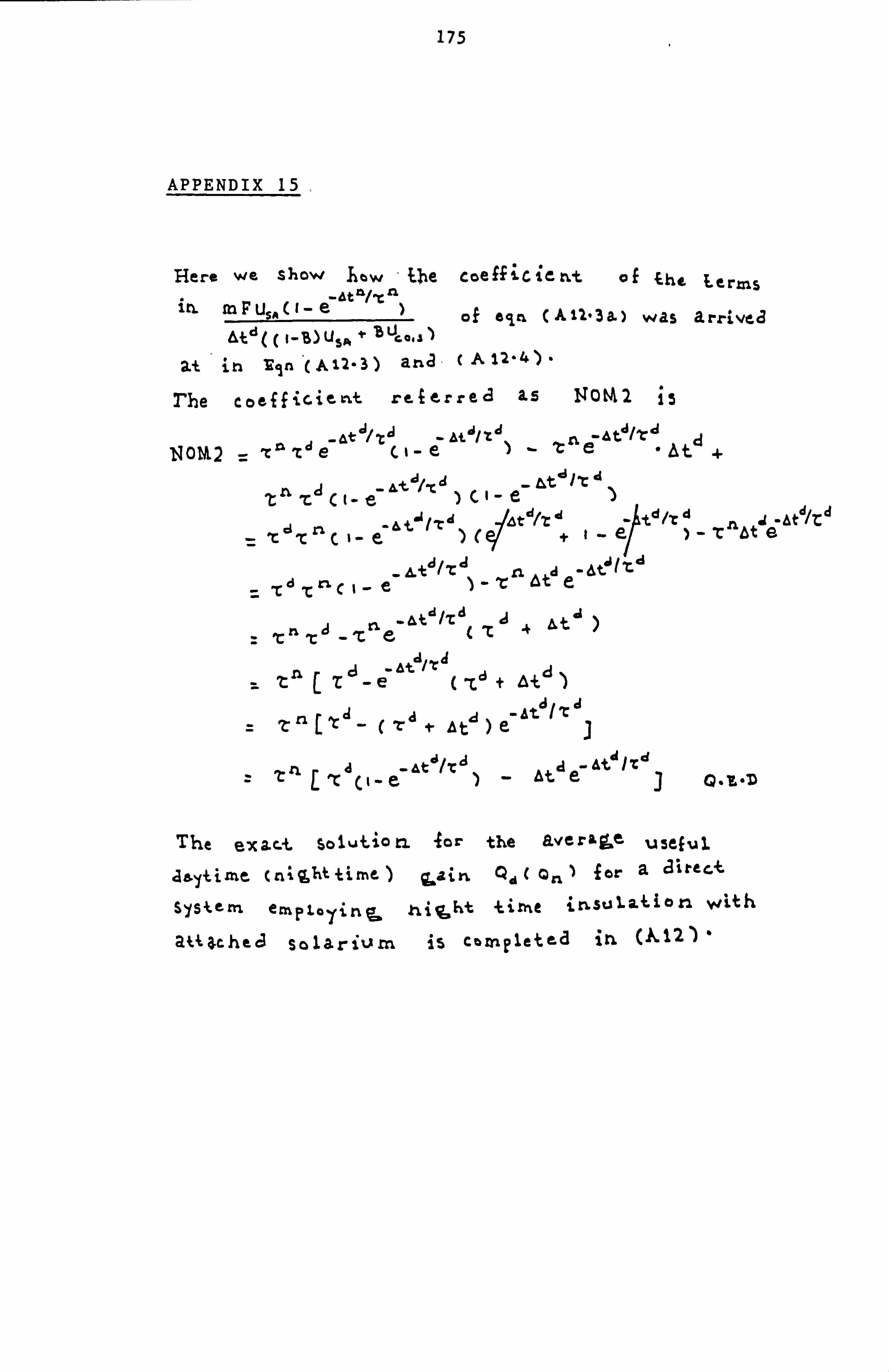
175

APPENDIX 15,

Hero we show hew tlipe coe Ef ic je r, + Of the Lerms "a F USA eat ftlýt

of ecla (All-3&) was arrive_, 3 , &4- d US4 Z U,

2-1 i rl vjn . (A 12- 3) aria, cA 12-4) -

rhe coefficitnt reietrred LS

-&t J/. Cj -

-C IqOm2 'cr, Elie (I- cl'eael 0 At d+

Ic A T_ c 4, tjz%d )ce b1tapt'i ) of Cý4td/zd

.t d/, r d

TcllrL, e-7&t +i- eý Ic bt 6 jd d Ic MC e cn Ae e-

rl j rl - atd/, rd C -t

j '+

At)

aE ci. atý/Tj ad zet At

Ic' -t

- 'r 11 ETaCI_ e_ At,,,, C

)_ &t ,

e7 Atý /. C djQ.,

L -'D

The exac. -L Solution for the iLver&j&t u3eful

, 1g. 1time (ni%littime) q.. & in QI( o. ) for a c3irec. +-

SISkem e ra a -Y ht 4_jrne jrsulation with

attache, 8 solarium is complete-(] 12

176

A16 Empirical fit of outlet to inlet area on perCent increase of. air flow due to wind and thermal forces V wind, ct&Cv-

__

The desired f it on the curve for -, ý ýws*g%je

vs A,,, t/AL, will be assumed of the form

A, t s AL

-ý 17

-t)=A,, V

where A6,, tand AL represent the '

ventilation outlet area and inlet respectively in -mL a%ý is the percentage increase in air

volume flow rate ("1/5) (wind and stack forces). Aj and ALare constants of the fit. See curve (17). Equation A16-4

reduces to 6 A -t ki -r

-DV - (A 116- 2.

JýZ' A!! z_, d . This is the linear form in the log

and log*aý variates with log A, being the intercept om the log ( AO-t axis. A, % is the slope of the curve. Equation A16.2 is a linear form, and linear

regression yields the coefficients

IAý3 A=1,. )Z C ýý -4)- At J-3 D

It

and

A2. )2/_n

where n is the data number. - 4(116-9+)

using equations A16.3 and A16.4 and data set from the curve (17) log Ai and A are easily evaluated as

177

A-L = 2-4 - (A 16-S)

1,33 Aj =-30 If 4- (A t(6- 6

From equation 16.2,16.5 and 16.6

Log( kt"ý 4 A4.

or log(

and 1, (A 16, q

Az, Rearranging equation A16.9 yields

A 1.4

AL 04

37 A W't c-19- 1- -(A IL-41

1.95

in equation A16.11 is a percentage increase, therefore

9ý= 0-4- '-T ( tLwt

-I) 06 3:? _

- (A i6-a)

From which too AL

Ao 2.4 1

Equation A16.13 presents us with the relation between the outlet, inlet area

(A*,, % /AL ) and the fraction increase in ventilation volume flow rate (, K, "jS)( due to unequivalent inlet, outlet areas). The areas measured in *n2 ,

178

The Order of Fit

In evalauating the fit, one dete. rmines the

, correlation coefficient of the V variate on the A&4: L/A.. * variate. The correlation coefficient being

I A t lot

A Aý

JW-4 AL

COS*

Using the predicted data sets one obtains

'r =a- 41 L+ -CA 16-5) t

Such a value of the coefficient of correlation indicates that the power form of equation A16.3 predicts the actual data sets with as good enough accuracy as any other. An ideal fit is characterised by a coefficient ( ylý= A-a ).

Table Aj(,. j has been constructed for purposes of comparison. It is seen that the predicted values by equation A16.13 compare sufficiently well with the actual data records. It is of particular interest to mention that the closest accuracy'in prediction ofaý occurs when the ratio between inlet and outlet area A6, -t /AL or vice versa is numerically four. This presents us with a possible design choice namely the area of the stack in the roof space (exit) is a fourth the inlet area (equivalent to area of open doors or windows in conservatory) in*4z Thus one selects,

AZ- 4- )e 'A ,t when using equation A16.13, and is reasonably safest. Figure 2.7 shows a plot of the predicted and monitored records.

L78 aL

LOIS

4. r

Ito 2,4-. r 1

114-2.

s 21.2

4- 3f,. 3

6 1 31 4-1- 3

C*)Ref. (17) curve,

,, eqn. 2.51; (r - 0.94),,, see A16. (+Ir-urve fit;

Table A16-1 Effect of outlet to inlet area Ao.

_. r /A;., on air flow due to

wind, and thermal forces,,,

179

A17 Fitted Curve for Ventilation air flow rate(YO/S) due to combined wind and stack forces as function of stack to combined flow rates (Fi. 2-9)

The curve to be fitted is presented in the ASHRAE handbook of fundamentals (17). The empirical form will be written as

lot

(A 44-1

where V&t,, Kis the ventilation pir flow rate due to thermal forces ); is the ventilation air flow rate due to wind forces (w4%). F,,, is the actual flow multiple on flow due to temperature difference. a and b are constants of the equation. Writing the second term of the L. H. S. of eqn. A17.1 as D,

1 10 0Lb-�,. t]]

"' E F� -11=b- (A at : ý. -2 )

In eqn. A17.2, D is the x variate and F, the y-variate. The equation A17.2ýhas two assym- todes on the lines D-0.1 and F.,, = 1, respectively.

The logarithmic form of equation A17.2 is

43 L 16 aI b- 0--t 3 3- 4, b= L*ý E V-M -II -(A 446 3

or by logarithmic-properties

C43L.. 3 [ý4oL tý, -a-iII- CA A-1 04 )

Equation A17.4 above is a linear form* The y variate is log (Fm-1), while the x-variate is log (46o4 b- b--i )). Log b and a are constants of the equation.

180

A linear regression of equation A17.4 yields the constants

Log 6= Lej E Fm -4]- 01. L-6-3 EI 00 ýV - 0-1 ]] -(A 17-5)

and La2l Cloo

LO-3 4ZO Ctl- 0-11 )2-(2: L4P3 tOl) Lb- 0-4 /Y1

whereIrl is the number of data sets.

Using equation A17.5 and A17.6 together with the data set (Ref. 17). log b and a are evaluated as

log b-2.526 - CA17.7)

a=1.9 - (A17.8 )

From equations A17.4, A17.7 and A17.8

Log Efým-, Q 2-526 I-on [100

or log 41 LOZ Ia

and -4-11

- (A 't:; -44) Rearrange eqn. A17.11 and

ass-S

Ito K.

toot

181

Again such value for equation A17.12 can level of confidence.

the fit order Td indicates be used with a comfortable

F. vv% as given by equation A17.12 is the multiplication factor on the ventilation air flow rate due to thermal forces This product for a given ratio of stack to combined ventilation flow rates represents the combination flow rate when stack and wind forces are considered.

v e. -tj . 4. D, aaCKI Ito [ %)&tacic + Sý%ae, -A

II

0 where

V verlt, wind, stack is obtained in (11-314) and

V stack (V wind) represent the volumetric flow rates by thermal and wind effects in (ro-11S).

Another inspection of that Fv., is a decayin combined flow rates. unity at, sufficiently combined flow rates. stack flow conditions to

equation (A17.12) reveals g function of stack to

This function decays to large values of stack to Thus, for predominant equation A17.14 reduces

0 IL

as should be expected.

Table A17.1 below has been constructed for purposes of

182

comparing the predictions by equation A17.12 and the monitored values (ref. 17) for various stack to combined flow rates.

-

oll,

S'o 1 1.2. ýq i 60 1 -

- -1-189

1

70 4-134

c«) Rti ci'el

(A 44-42)

r,. = -O. qq-

Table A17.1. Predicted and monitored values of the multiplication factor F,,,,

Again, a choice of o 14 Lt4+ s,, a +1 ýSt&cx- +

the empirical form A17.12. This suits situations normally encountered in practice, as the stack effects will more commonly dominate the wind forces.

183

A18 Solution of the Energy Balance Equation of Building Envelop

The following equation is to be solved (eqn. 2.6)

ýCp ý-Tt -

[(BFcQ, 4- (1 -1)? QT) - uti(Tt -Ta, )]= 0(P, IR-1 ) dt

OR dTf

+ L-l"I Tf C S'F, Or +CI -B) FG U4Lq Ta2

. 1-L filcy in C? iRt

of form

dj + cjý C0 'd -=

(P.

dV k. C, CX 15-14)

d%

X C1,4 d4 CIZ C

tj X

e+2 d: c

a P. eel*'

Integrating both sides w. r. t. CIX

9e e-

+CX je-7

C'x C2 + r- e C,

U41 Tj

ST, a+ (I-B)FOr 4 Ce

( rilep I( U*'J I Lix CI (AiS-9)

or T, -Ta BFc; T + us., +Ci the?

( AIS-10

We apply the condition that at inlet, when the fluid temperature is the conservatory temperature T

to 0

IN 1111111111111111111111 1401614509 · 2013. 6. 4. · 2.25 Heat removal factor FR of building...

Documents

Transcript of IN 1111111111111111111111 1401614509 · 2013. 6. 4. · 2.25 Heat removal factor FR of building...