Imputation Techniques For Market Research Datasets With Missing Values

Imputation of Time Series with MissingValues under Heavy-Tailed AR Model via
Stochastic EM
Prof. Daniel P. PalomarThe Hong Kong University of Science and Technology (HKUST)
Invited Talk - International Workshop onMathematical Issues in Information Sciences (MIIS)The Chinese University of Hong Kong, Shenzhen
21 December 2018

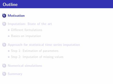
Outline
1 Motivation
2 Imputation: State of the art
Different formulationsBasics on imputation
3 Approach for statistical time series imputation
Step 1: Estimation of parametersStep 2: Imputation of missing values
4 Numerical simulations
5 Summary
Outline
1 Motivation
2 Imputation: State of the art
Different formulationsBasics on imputation
3 Approach for statistical time series imputation
Step 1: Estimation of parametersStep 2: Imputation of missing values
4 Numerical simulations
5 Summary

Data with missing values
In theory, data is typically assumed complete and algorithms aredesigned for complete data.In practice, however, often data has missing values, due to avariety of reasons.Then the algorithms designed for complete data can be disastrous!Missing values typically happen during the data observation orrecording process:1
values may not be measured,values may be measured but get lost, orvalues may be measured but are considered unusable.
1R. J. Little and D. B. Rubin, Statistical Analysis with Missing Data, 2nd Ed.Hoboken, N.J.: John Wiley & Sons, 2002.
D. Palomar (HKUST) Imputation of Time Series 4 / 42

Data with missing values
Some real-world cases where missing values occur:some stocks may suffer a lack of liquidity resulting in no transactionand hence no price recordedobservation devices like sensors may break down during themeasurementweather or other conditions may disturb sample taking schemesin industrial experiments some results may be missing because ofmechanical breakdowns unrelated to the experimental processin an opinion survey some individuals may be unable to express apreference for one candidate over anotherrespondents in a survey may not answer every questioncountries may not collect statistics every yeararchives may simply be incompletesubjects may drop out of panels.
D. Palomar (HKUST) Imputation of Time Series 5 / 42
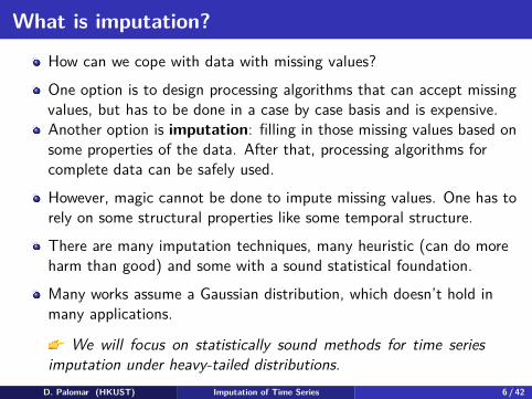
What is imputation?
How can we cope with data with missing values?One option is to design processing algorithms that can accept missingvalues, but has to be done in a case by case basis and is expensive.Another option is imputation: filling in those missing values based onsome properties of the data. After that, processing algorithms forcomplete data can be safely used.However, magic cannot be done to impute missing values. One has torely on some structural properties like some temporal structure.There are many imputation techniques, many heuristic (can do moreharm than good) and some with a sound statistical foundation.Many works assume a Gaussian distribution, which doesn’t hold inmany applications.
We will focus on statistically sound methods for time seriesimputation under heavy-tailed distributions.
D. Palomar (HKUST) Imputation of Time Series 6 / 42

Outline
1 Motivation
2 Imputation: State of the art
Different formulationsBasics on imputation
3 Approach for statistical time series imputation
Step 1: Estimation of parametersStep 2: Imputation of missing values
4 Numerical simulations
5 Summary

Outline
1 Motivation
2 Imputation: State of the art
Different formulationsBasics on imputation
3 Approach for statistical time series imputation
Step 1: Estimation of parametersStep 2: Imputation of missing values
4 Numerical simulations
5 Summary
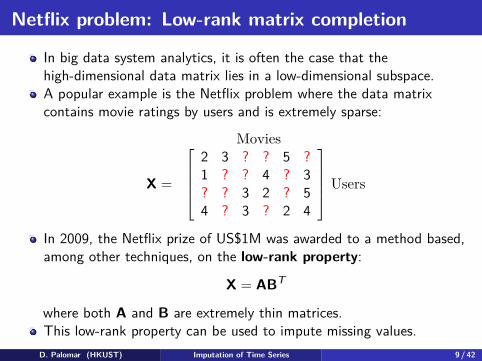
Netflix problem: Low-rank matrix completion
In big data system analytics, it is often the case that thehigh-dimensional data matrix lies in a low-dimensional subspace.A popular example is the Netflix problem where the data matrixcontains movie ratings by users and is extremely sparse:
Movies
X =
2 3 ? ? 5 ?1 ? ? 4 ? 3? ? 3 2 ? 54 ? 3 ? 2 4
Users
In 2009, the Netflix prize of US$1M was awarded to a method based,among other techniques, on the low-rank property:
X = ABT
where both A and B are extremely thin matrices.This low-rank property can be used to impute missing values.
D. Palomar (HKUST) Imputation of Time Series 9 / 42
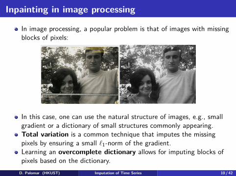
Inpainting in image processing
In image processing, a popular problem is that of images with missingblocks of pixels:
In this case, one can use the natural structure of images, e.g., smallgradient or a dictionary of small structures commonly appearing.Total variation is a common technique that imputes the missingpixels by ensuring a small ℓ1-norm of the gradient.Learning an overcomplete dictionary allows for imputing blocks ofpixels based on the dictionary.
D. Palomar (HKUST) Imputation of Time Series 10 / 42
Frugal sensing and compressive covariance sensing
A somehow related problem in signal processing and wirelesscommunications is frugal sensing and compressive covariance sensingwhere one wants to obtain the complete knowledge of a covariancematrix.In frugal sensing,2 one wants to obtain the matrix X from knowledgeof the value of some cuts cT
i Xci = vi or even just one bit ofinformation of the cuts cT
i Xci ≶ t.More generally, in compressive covariance sensing,3 one wants toreconstruct X from the smaller matrix CTXC, where C is some tallcompression or selection matrix that exploits structural information orsparsity in some domain.
2O. Mehanna and N. Sidiropoulos, “Frugal sensing: Wideband power spectrumsensing from few bits,” IEEE Trans. on Signal Processing, vol. 61, no. 10,pp. 2693–2703, 2013.
3D. Romero, D. D. Ariananda, Z. Tian, and G. Leus, “Compressive covariancesensing: Structure-based compressive sensing beyond sparsity,” IEEE Signal ProcessingMagazine, vol. 33, no. 1, pp. 78–93, 2016.
D. Palomar (HKUST) Imputation of Time Series 11 / 42

Time series with structureIn some applications, one of the dimensions of the data matrix is time.The time dimension sometimes has some specific structure on thedistribution of the missing values, like the monotone missing pattern.4The time dimension can also follow some structural model that canbe effectively used to fill in the missing values.One simple example of time structure is the random walk, which ispervasive in financial applications (e.g., log-returns of stocks):5
yt = ϕ0 + yt−1 + εt.
Another example of time structure is the AR(p) model (e.g.,traded log-volume of stocks):
yt = ϕ0 +p∑
i=1ϕiyt−i + εt.
4J. Liu and D. P. Palomar, “Robust estimation of mean and covariance matrix forincomplete data in financial applications,” in Proc. IEEE GlobalSIP, Montreal, Canada,2017.
5J. Liu, S. Kumar, and D. P. Palomar, “Parameter estimation of heavy-tailed randomwalk model from incomplete data,” in Proc. IEEE International Conference on Acoustics,Speech and Signal Processing (ICASSP), Calgary, Alberta, Canada, 2018.
D. Palomar (HKUST) Imputation of Time Series 12 / 42

Outline
1 Motivation
2 Imputation: State of the art
Different formulationsBasics on imputation
3 Approach for statistical time series imputation
Step 1: Estimation of parametersStep 2: Imputation of missing values
4 Numerical simulations
5 Summary
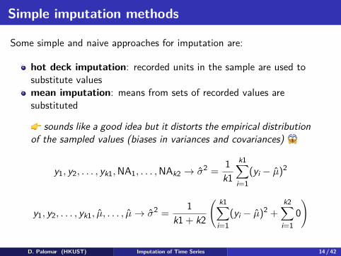
Simple imputation methods
Some simple and naive approaches for imputation are:
hot deck imputation: recorded units in the sample are used tosubstitute valuesmean imputation: means from sets of recorded values aresubstituted
sounds like a good idea but it distorts the empirical distributionof the sampled values (biases in variances and covariances)
y1, y2, . . . , yk1,NA1, . . . ,NAk2 → σ2 = 1k1
k1∑i=1
(yi − µ)2
y1, y2, . . . , yk1, µ, . . . , µ→ σ2 = 1k1 + k2
( k1∑i=1
(yi − µ)2 +k2∑
i=10)
D. Palomar (HKUST) Imputation of Time Series 14 / 42

Naive vs sound imputation methods
Ad-hoc methods of imputation can lead to serious biases in variancesand covariances.Examples are:
mean imputationconstant interpolationlinear interpolationpolynomial interpolationspline interpolation
A sound imputation method should preserve the statistics of theobserved values.
The statistical way is to first estimate the distribution of themissing values conditional on the observed values f (ymiss|yobs)and then impute based on that posterior distribution.
D. Palomar (HKUST) Imputation of Time Series 15 / 42

Naive vs sound time series imputation methodsIllustration of different naive imputation methods and a sound statisticalmethod that preserves the statistics:
Jan 03
2012
Jul 02
2012
Jan 02
2013
Jul 01
2013
Jan 02
2014
Jul 01
2014
Jan 02
2015
Jun 30
2015
7.2
7.3
7.4
7.5
7.6
Imputation with LOCF (last observation carried forward)
Jan 03
2012
Jul 02
2012
Jan 02
2013
Jul 01
2013
Jan 02
2014
Jul 01
2014
Jan 02
2015
Jun 30
2015
7.2
7.3
7.4
7.5
7.6
Imputation with linear interpolation
Jan 03
2012
Jul 02
2012
Jan 02
2013
Jul 01
2013
Jan 02
2014
Jul 01
2014
Jan 02
2015
Jun 30
2015
7.2
7.3
7.4
7.5
7.6
Imputation with splines
Jan 03
2012
Jul 02
2012
Jan 02
2013
Jul 01
2013
Jan 02
2014
Jul 01
2014
Jan 02
2015
Jun 30
2015
7.2
7.3
7.4
7.5
7.6
Imputation with proposed method (statistics preserved)
D. Palomar (HKUST) Imputation of Time Series 16 / 42

Single and multiple imputation
Suppose we have somehow estimated the conditional distributionf (ymiss|yobs).At this point it is trivial to randomly generate the missing values fromthat distribution:
ymiss ∼ f (ymiss|yobs).
This only gives you one realization of the missing values.In some applications, one would like to have multiple realizations ofthe missing values to properly test the performance of somesubsequent methods or algorithms.Multiple imputation (MI) consists of generating multiple realizationsof the missing values:
y(k)miss ∼ f (ymiss|yobs) ∀k = 1, . . . ,K.
D. Palomar (HKUST) Imputation of Time Series 17 / 42
Outline
1 Motivation
2 Imputation: State of the art
Different formulationsBasics on imputation
3 Approach for statistical time series imputation
Step 1: Estimation of parametersStep 2: Imputation of missing values
4 Numerical simulations
5 Summary
Outline
1 Motivation
2 Imputation: State of the art
Different formulationsBasics on imputation
3 Approach for statistical time series imputation
Step 1: Estimation of parametersStep 2: Imputation of missing values
4 Numerical simulations
5 Summary

Estimation of parameters for iid Gaussian
Suppose a univariate random variable y follows a Gaussiandistribution:
y ∼ N(µ, σ2
).
We have T incomplete samples {yt} and the missing mechanism isignorable (aka MAR), the ML estimation problem is formulated as
maximizeµ,σ2
log(∏
t∈Cobs fG(yt;µ, σ2))
,
where Cobs is the set of the indexes of the observed samples, andfG (·) is the pdf of the Gaussian distribution.Closed-form solution:
µ = 1nobs
∑t∈Cobs
yt
andσ2 = 1
nobs
∑t∈Cobs
(yt − µ)2 .
D. Palomar (HKUST) Imputation of Time Series 20 / 42

Estimation of parameters for iid Student’s tIn many applications, the Gaussian distribution is not appropriateand a more realistic heavy-tailed distribution is necessary.An example is in the financial returns of stocks:
Histogram of S&P 500 log−returns
return
Den
sity
−0.06 −0.04 −0.02 0.00 0.02 0.04
010
2030
4050
6070 Gaussian fit
D. Palomar (HKUST) Imputation of Time Series 21 / 42

Estimation of parameters for iid Student’s tThe Student’s t-distribution is a widely used heavy-tailed distribution.Suppose y follows a Student’s t-distribution: y ∼ t
(µ, σ2, ν
)with pdf
ft(y;µ, σ2, ν
)=
Γ(
ν+12
)√νπσΓ
(ν2) (1 + (y− µ)2
νσ2
).
Given the incomplete data set, the ML estimation problem forθ =
(µ, σ2, ν
)can be formulated as
maximizeµ,σ2,ν
log(∏
t∈Cobs ft(yt;µ, σ2, ν
)).
No closed-form solution.Interestingly, the Student’s t-distribution can be represented as aGaussian mixture:
yt|τt ∼ N(µ,σ2
τt
), τt ∼ Gamma
(ν
2 ,ν
2
),
where τt is the mixture weight.D. Palomar (HKUST) Imputation of Time Series 22 / 42
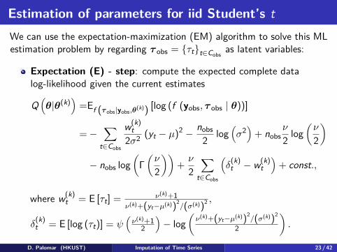
Estimation of parameters for iid Student’s tWe can use the expectation-maximization (EM) algorithm to solve this MLestimation problem by regarding τ obs = {τt}t∈Cobs
as latent variables:
Expectation (E) - step: compute the expected complete datalog-likelihood given the current estimates
Q(θ|θ(k)
)=Ef (τ obs|yobs,θ
(k)) [log (f (yobs, τ obs | θ))]
=−∑
t∈Cobs
w(k)t
2σ2 (yt − µ)2 − nobs2 log
(σ2)
+ nobsν
2 log(ν
2
)
− nobs log(
Γ(ν
2
))+ ν
2∑
t∈Cobs
(δ
(k)t − w(k)
t)
+ const.,
where w(k)t = E [τt] = ν(k)+1
ν(k)+(yt−µ(k))2/(σ(k))2 ,
δ(k)t = E [log (τt)] = ψ
(ν(k)+1
2
)− log
(ν(k)+(yt−µ(k))2
/(σ(k))2
2
).
D. Palomar (HKUST) Imputation of Time Series 23 / 42

Estimation of parameters for iid Student’s t
Maximization (M) - step: update the estimates as
θ(k+1) = argmaxθ
Q(θ|θ(k)
)and has closed-form solution:
µ(k+1) =∑
t∈Cobs w(k)t yt∑
t∈Cobs w(k)t
,
(σ(k+1)
)2=∑
t∈Cobs w(k)t(yt − µ(k+1)
)2
nobs,
ν(k+1) = argmaxν>0
nobs
(ν
2 log(ν
2
)− log
(Γ(ν
2
)))+ ν
2∑
t∈Cobs
(δ
(k)t − w(k)
t).
D. Palomar (HKUST) Imputation of Time Series 24 / 42

AlgorithmStochastic EM algorithm for iid Student’s t:
Initialize µ(0),(σ(0)
)2, and ν(0). Set k = 0.
repeat
w(k)t = ν(k) + 1
ν(k) +(yt − µ(k))2 / (σ(k))2 ,
µ(k+1) =∑
t∈Cobs w(k)t yt∑
t∈Cobs w(k)t
,
(σ(k+1)
)2=∑
t∈Cobs w(k)t(yt − µ(k+1)
)2
nobs,
ν(k+1) = argmaxν>0
Q(µ(k+1),
(σ(k+1)
)2, ν|µk,
(σk)2, νk)
k← k + 1until convergence
D. Palomar (HKUST) Imputation of Time Series 25 / 42

Estimation of parameters for AR(1) Student’s t
Consider an AR(1) time series with innovations following a Student’st-distribution:
yt = φ0 + φ1yt−1 + εt,
where εt ∼ t(0, σ2, ν
).
The ML estimation problem for θ =(φ0, φ1, σ2, ν
)is formulated as
maximizeϕ0,φ1,σ2,ν
log(∫ ∏T
t=2 ft(yt;φ0 + φ1yt−1, σ2, ν
)dymiss
)The objective function involves an integral, and we have noclosed-form expression.As before, we can represent εt as
εt|τt ∼ N(
0, σ2
τt
), τt ∼ Gamma
(ν
2 ,ν
2
),
and use the EM type algorithm to solve this optimization problem byregarding ymiss and τ = {τt}t=1,...,T as the latent variables.
D. Palomar (HKUST) Imputation of Time Series 26 / 42

Estimation of parameters for AR(1) Student’s tThe complete data log-likelihood f (yobs, ymiss, τ | θ) belongs to theexponential family:
f (yobs, ymiss, τ | θ)=h (yobs, ymiss, τ ) exp (−ψ (θ) + ⟨s (yobs, ymiss, τ ) ,ϕ (θ)⟩)
where
h (yobs, ymiss, τ ) =T∏
t=2τ
− 12
t ,
ψ (θ) = − (T− 1){ν
2 log(ν
2
)−log
(Γ(ν
2
))−1
2 log(σ2)−1
2 log (2π)},
s (yobs, ymiss, τ ) =T∑
t=2
[log (τt)−τt, τty2
t , τt, τty2t−1, τtyt, τtytyt−1, τtyt−1
],
ϕ (θ) =[ν
2 , −1
2σ2 , −φ2
02σ2 , −
φ21
2σ2 ,φ0σ2 ,
φ1σ2 , −
φ0φ1σ2
].
D. Palomar (HKUST) Imputation of Time Series 27 / 42
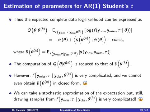
Estimation of parameters for AR(1) Student’s t
Thus the expected complete data log-likelihood can be expressed as
Q(θ|θ(k)
)=Ef (ymiss,τ |yobs,θ
(k)) [log (f (yobs, ymiss, τ | θ))]
=− ψ (θ) +⟨s(θ(k)
),ϕ (θ)
⟩+ const.,
where s(θ(k)
)= Ef (ymiss,τ |yobs,θ
(k)) [s (yobs, ymiss, τ )].
The computation of Q(θ|θ(k)
)is reduced to that of s
(θ(k)
).
However, f(ymiss, τ | yobs,θ
(k))
is very complicated, and we cannoteven obtain s
(θ(k)
)in closed form.
We can take a stochastic approximation of the expectation but, still,drawing samples from f
(ymiss, τ | yobs,θ
(k))
is very complicated!
D. Palomar (HKUST) Imputation of Time Series 28 / 42
Estimation of parameters for AR(1) Student’s t
We will use a Markov chain Monte Carlo (MCMC) process.
In particular, we consider the Gibbs sampling method to generate theMarkov chain: we divide the latent variables (ymiss, τ ) into two blocksτ and ymiss and then generate a Markov chain of samples from theconditional distributions f
(τ |ymiss, yobs,θ
(k))
andf(ymiss|τ , yobs,θ
(k))
alternatively:
Drawing from f(τ |ymiss, yobs,θ
(k))
is trivial since the elementsof τ are iid following a univariate gamma distribution.
Drawing from f(ymiss|τ , yobs,θ
(k))
is trivial since it’s just aGaussian distribution.
D. Palomar (HKUST) Imputation of Time Series 29 / 42

Algorithm
Stochastic EM algorithm for AR(1) Student’s t:Initialize latent variables and set k = 0.repeat
Simulation step: generate the samples(τ (k,l), y(k,l)
m)
(l = 1, 2 . . . , L)
from f(ymiss, τ |yobs; θ(k)
)via Gibbs sampling (L parallel chains).
Approximation step:
s(k) = s(k−1) + γ(k)(
1L
L∑l=1
s(yobs, y(k,l)
miss, τ(k,l))− s(k−1)
).
Maximization step: θ(k+1) = argmaxθ
Q(θ, s(k)
).
k← k + 1until convergence
D. Palomar (HKUST) Imputation of Time Series 30 / 42
Maximization step
The maximization step θ(k+1) = argmaxθ
Q(θ, s(k)
)can be obtained in
closed form:
φ(k+1)0 = s(k)
5 − φ(k+1)1 s(k)
7
s(k)3
,
φ(k+1)1 = s(k)
3 s(k)6 − s(k)
5 s(k)7
s(k)3 s(k)
4 −(s(k)7)2 ,
(σ(k+1)
)2= 1
T− 1
(s(k)2 +
(φ
(k+1)0
)2s(k)3 +
(φ
(k+1)1
)2s(k)4
− 2φ(k+1)0 s(k)
5 − 2φ(k+1)1 s(k)
6 + 2φ(k+1)0 φ
(k+1)1 s(k)
7
),
ν(k+1) = arg maxν>0
(T− 1){ν
2 log(ν
2
)− log
(Γ(ν
2
))}+ ν s(k)
12 .
D. Palomar (HKUST) Imputation of Time Series 31 / 42

Convergence
The previous algorithm is very simple but does it converge?
Theorem:
The sequence{
θ(k)}
generated by the algorithm has the followingasymptotic property: with probability 1, limk→+∞ d
(θ(k),L
)= 0, where
d(θ(k),L
)denotes the distance from θ(k) to the set of stationary points
of observed data log-likelihood L ={
θ ∈ Θ, ∂l(θ;yobs)∂θ = 0
}.a
aJ. Liu, S. Kumar, and D. P. Palomar, “Parameter estimation of heavy-tailedAR model with missing data via stochastic EM,” arXiv preprint, 2018. [Online].Available: https://arxiv.org/pdf/1809.07203.pdf.
D. Palomar (HKUST) Imputation of Time Series 32 / 42

Outline
1 Motivation
2 Imputation: State of the art
Different formulationsBasics on imputation
3 Approach for statistical time series imputation
Step 1: Estimation of parametersStep 2: Imputation of missing values
4 Numerical simulations
5 Summary
Step 2: Imputation of missing values
Given the conditional distribution f (ymiss|yobs), it is trivial torandomly generate the missing values (multiple realizations can bedrawn for multiple imputation):
ymiss ∼ f (ymiss|yobs).However, in our case, we don’t have the conditional distributionf (ymiss|yobs) in closed form:
f (ymiss|yobs) =∫
f (ymiss|yobs,θ)f (θ|yobs)dθ
An improper way of imputing (which is acceptable in many cases withsmall percentage of missing values) is with f (ymiss|yobs,θ
ML), buteven that expression is not available.We can instead draw from f (ymiss, τ |yobs,θ
ML) and discard τ , butthat expression is not available either.
We can generate the samples from the joint based on Markovchains.
D. Palomar (HKUST) Imputation of Time Series 34 / 42

Step 2: Imputation of missing values
In particular, we consider the Gibbs sampling method to generate theMarkov chain: we divide the latent variables (ymiss, τ ) into two blocksτ and ymiss and then generate a Markov chain of samples from theconditional distributions f (τ |ymiss, yobs,θ) and f (ymiss|τ , yobs,θ)alternatively.
Drawing from f (τ |ymiss, yobs,θ) is trivial since the elementsof τ are iid, so it is just a univariate gamma distribution for eachelement.
Drawing from f (ymiss|τ , yobs,θ) is just a Gaussian distribution.
If multiple imputation is needed, then the Markov chain has to begenerated multiple times. But this is not the correct way to domultiple imputation!
The correct way is via a Bayesian characterization of θ insteada point estimation like ML.
D. Palomar (HKUST) Imputation of Time Series 35 / 42

Outline
1 Motivation
2 Imputation: State of the art
Different formulationsBasics on imputation
3 Approach for statistical time series imputation
Step 1: Estimation of parametersStep 2: Imputation of missing values
4 Numerical simulations
5 Summary

Numerical simulationsEstimation of parameters for AR(1) Student’s t with real data (S&P 500):
0.00
60.
012
φ 00.
9980
0.99
88
φ 13.
5e−
055.
0e−
05
σ2
0 20 40 60 80 100
3.0
4.0
5.0
Iteration k
ν
D. Palomar (HKUST) Imputation of Time Series 37 / 42
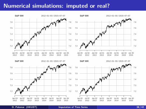
Numerical simulations: imputed or real?
Jan 032012
Jul 022012
Jan 022013
Jul 012013
Jan 022014
Jul 012014
Jan 022015
Jun 302015
S&P 500 2012−01−03 / 2015−07−07
7.2
7.3
7.4
7.5
7.6
7.2
7.3
7.4
7.5
7.6
Jan 032012
Jul 022012
Jan 022013
Jul 012013
Jan 022014
Jul 012014
Jan 022015
Jun 302015
S&P 500 2012−01−03 / 2015−07−07
7.2
7.3
7.4
7.5
7.6
7.2
7.3
7.4
7.5
7.6
Jan 032012
Jul 022012
Jan 022013
Jul 012013
Jan 022014
Jul 012014
Jan 022015
Jun 302015
S&P 500 2012−01−03 / 2015−07−07
7.2
7.3
7.4
7.5
7.6
7.2
7.3
7.4
7.5
7.6
Jan 032012
Jul 022012
Jan 022013
Jul 012013
Jan 022014
Jul 012014
Jan 022015
Jun 302015
S&P 500 2012−01−03 / 2015−07−07
7.2
7.3
7.4
7.5
7.6
7.2
7.3
7.4
7.5
7.6
D. Palomar (HKUST) Imputation of Time Series 38 / 42

Numerical simulations: imputed or real?
Jan 032012
Jul 022012
Jan 022013
Jul 012013
Jan 022014
Jul 012014
Jan 022015
Jun 302015
S&P 500 2012−01−03 / 2015−07−07
7.2
7.3
7.4
7.5
7.6
7.2
7.3
7.4
7.5
7.6
Jan 032012
Jul 022012
Jan 022013
Jul 012013
Jan 022014
Jul 012014
Jan 022015
Jun 302015
S&P 500 2012−01−03 / 2015−07−07
7.2
7.3
7.4
7.5
7.6
7.2
7.3
7.4
7.5
7.6
Jan 032012
Jul 022012
Jan 022013
Jul 012013
Jan 022014
Jul 012014
Jan 022015
Jun 302015
S&P 500 2012−01−03 / 2015−07−07
7.2
7.3
7.4
7.5
7.6
7.2
7.3
7.4
7.5
7.6
Jan 032012
Jul 022012
Jan 022013
Jul 012013
Jan 022014
Jul 012014
Jan 022015
Jun 302015
S&P 500 2012−01−03 / 2015−07−07
7.2
7.3
7.4
7.5
7.6
7.2
7.3
7.4
7.5
7.6
D. Palomar (HKUST) Imputation of Time Series 39 / 42
Outline
1 Motivation
2 Imputation: State of the art
Different formulationsBasics on imputation
3 Approach for statistical time series imputation
Step 1: Estimation of parametersStep 2: Imputation of missing values
4 Numerical simulations
5 Summary

Summary
We have introduced the issue of missing values in observations.Imputation is the mechanism by which one fills in those missingvalues.Many methods are ad-hoc with no good statistical results.Other methods are based on some properly defined formulation basedon some structural properties of the data matrix.Time series contain special temporal structure that can be employedfor imputation.Sound statistical method:
1 estimate the statistics of the underlying distribution function andconstruct the conditional distribution
2 impute based on the conditional distribution either a single time ormultiple times (multiple imputation)
D. Palomar (HKUST) Imputation of Time Series 41 / 42

Thanks
For more information visit:
https://www.danielppalomar.com