Improving the simulation of small-scale variability in ...hss.ulb.uni-bonn.de/2011/2632/2632.pdf ·...
122
Improving the simulation of small-scale variability in radiation and land-surface parameterizations in a mesoscale numerical weather prediction model Dissertation zur Erlangung des Doktorgrades (Dr. rer. nat.) der Mathematisch-Naturwissenschaftlichen Fakultät der Rheinischen Friedrich-Wilhelms-Universität Bonn vorgelegt von Annika Schomburg aus Braunschweig Bonn, Februar 2011
Transcript of Improving the simulation of small-scale variability in ...hss.ulb.uni-bonn.de/2011/2632/2632.pdf ·...
Improving the simulation of
small-scale variability in radiation
and land-surface parameterizations
in a mesoscale numerical weather
prediction model
Dissertationzur
Erlangung des Doktorgrades (Dr. rer. nat.)der
Mathematisch-Naturwissenschaftlichen Fakultätder
Rheinischen Friedrich-Wilhelms-Universität Bonn
vorgelegt vonAnnika Schomburg
ausBraunschweig
Bonn, Februar 2011

Angefertigt mit Genehmigung der Mathematisch-Naturwissenschaftlichen Fakultät derRheinischen Friedrich-Wilhelms-Universität Bonn
1. Gutachter: Prof. Dr. Clemens Simmer
2. Gutachter: Prof. Dr. Andreas Bott
Tag der Promotion: 26. Juli 2011
Erscheinungsjahr: 2011

Zusammenfassung
Zur Simulation von subskaligen physikalischen Prozessen in numerischen Wettervorher-sagemodellen werden eine Reihe von Vereinfachungen und Annahmen angewandt, umRechenzeit zu sparen. Dies gilt zum einen für die Simulation der Prozesse innerhalbder physikalischen Parametrisierungen, aber auch für die räumliche und zeitliche Fre-quenz der Aufrufe dieser Parametrisierungen. Die so verursachte Vernachlässigung vonkleinskaliger Variabilität kann zu systematischen Fehlern aufgrund der Nichtlinearitätenin den physikalischen Prozessen und zu Inkonsistenzen zwischen den Variablen aus denunterschiedlichen Parametrisierungen führen.
In dieser Arbeit werden zwei Methoden vorgestellt, die eine effizientere Berücksichti-gung von Heterogenitäten in Atmosphärenmodellen ermöglichen, zum einen innerhalb derAtmosphäre selbst, zum anderen an der Erdoberfläche als untere Randbedingung für dieAtmosphäre. Die erste Methode, die adaptive Strahlungstransportparametrisierung, isteine effektive Methode zur Berechnung der Strahlungseffekte in der Atmosphäre und ander Landoberfläche und führt zu einer Verbesserung der Erfassung von kurzfristigen klein-skaligen Änderungen im Wolkenfeld in Bezug auf Strahlungseffekte. Die zweite Methodehat das Ziel einer skalenkonsistenten Kopplung von Atmosphären- und Landoberflächen-modellen durch die Kopplung eines hochaufgelösten Boden-Vegetations-Transfermodellsan das gröbere atmosphärische Modell, wobei der atmosphärische Antrieb mit Hilfe einesin dieser Arbeit entwickelten Downscalings auf die kleine Skala disaggregiert wird. BeideMethoden führen zu einer verbesserten Berechnung der Energiebilanz an der Landober-fläche; erstere durch eine realistischere Simulation der Strahlungsflüsse, zweitere durchVerbesserung der turbulenten Flüsse sensibler und latenter Wärme. Beide Ansätze wur-den in das numerische Wettervorhersagemodell implementiert und in der COSMO-DEModellkonfiguration auf einem Gitter mit 2.8 km horizontalem Gitterabstand getestet.
Das Konzept der adaptiven Strahlungstransportparametrisierung macht sich die räum-lichen und zeitlichen Korrelationen in den optischen Eigenschaften der Atmosphäre zunutze,wodurch eine effizientere Ausnutzung der verfügbaren Rechenzeit möglich ist. AktuelleStrahlungsrechnungen basierend auf dem COSMO-internen komplexen Strahlungscode(basierend auf einem δ-Zweistromverfahren), die jeweils in einem Teil der Gitterpunktevorliegen, werden ausgenutzt, um möglichst realistische Strahlungsinformationen an denrestlichen Gitterpunkten zu erhalten. Zur Validierung dieses Schemas wurden drei Fallstu-dien mit unterschiedlichen synoptischen Bedingungen gerechnet, und die Ergebnisse desadaptiven Schemas mit Ergebnissen für das COSMO-DE-Standardschema verglichen, inwelches komplexe Strahlungsrechnungen viertelstündlich auf einem vergröberten Gitteraufgerufen werden. Als Referenz wurden häufige Strahlungsrechnungen auf dem kom-pletten dreidimensionalen Gitter durchgeführt. Die Ergebnisse zeigen, dass das adap-tive Schema in der Lage ist, die Sampling-Fehler des Standard-Verfahrens in den Netto-Strahlungsflüssen an der Landoberfläche deutlich zu reduzieren, und im Gegensatz zumoperationellen COSMO-DE-Verfahren die räumliche Variabilität in den Strahlungseffekten
3

4
korrekt zu simulieren. Fehler in den dreidimensionalen Heizraten werden auf größere Mit-telungsskalen verringert. Auch physikalische Zusammenhänge zwischen den Strahlungs-größen und Wolkenwasser oder Regenraten werden besser erfasst als mit dem Standard-schema. Es wird gezeigt, dass diese Verbesserungen auch einen positiven Einfluss auf diedynamische Modellentwicklung haben: Modellläufe, die mit adaptiver Strahlung gerech-net werden, weichen weit weniger von den Referenzläufen ab.
Eine Methode um subskalige Variabilität an der Erdoberfläche in atmosphärischen Mod-ellen zu berücksichtigen, ist der so genannte Mosaik-Ansatz. Beim Mosaik-Ansatz wird derBoden und die Erdoberfläche auf einer explizit höheren Auflösung gerechnet als der atmo-sphärische Teil. In der vorliegenden Arbeit wurde ein statistisches Downscaling-Verfahrenfür die atmosphärischen Antriebsvariablen für dieses höher aufgelöste Boden-Vegetations-Atmosphären-Transfermodul entwickelt, um eine skalen-konsistente zwei-Wege Kopplungzwischen den beiden Sub-Systemen Atmosphäre und Erdboden/Landoberfläche unter-schiedlicher Gitterweite im Mosaik-Ansatz zu ermöglichen. Dieses Disaggregationsschemakombiniert deterministische mit stochastischer Modellierung in einem schrittweisen Down-scaling Verfahren. Im ersten Schritt werden bi-quadratische Splines zur Interpolation vonder groben zur feinen Skala verwendet. Im zweiten Schritt werden Zusammenhänge zwis-chen atmosphärischen Variablen als Prädiktanden und Oberflächenparametern as Prädik-toren, abhängig vom Atmosphärenzustand, ausgenutzt. Im letzten Schritt wird die real-istische kleinskalige Varianz abgeschätzt, und die fehlende Variabilität als autoregressivesRauschen generiert und hinzugefügt. Dieses Disaggregationsverfahren wurde basierendauf hoch-aufgelöstem Modelloutput aus COSMO-Modellsimulationen mit 400m horizon-taler Gitterweite entwickelt und validiert, dazu wurde ein automatisches Regel-Such-System entwickelt. Das Verfahren wurde extensiv “offline” getestet, d.h. angewendet aufModelloutput, aber auch “online”, d.h. in das mesoskalige COSMO-Modell implementiertund eine Reihe von Fallstudien durchgeführt.
Angewendet auf die atmosphärischen Variablen der untersten COSMO-Modellschichtist das Disaggregationsschema in der Lage, die Referenzfelder adäquat zu rekonstruieren.Durch die beiden deterministischen Downscaling-Schritte werden Fehler reduziert, derstochastische Downscaling-Schritt führt zu einer guten Rekonstruktion der subskaligenVarianz, jeweils in Bezug zu hochaufgelösten Referenz-Feldern.
Es wird gezeigt, dass der Mosaik-Ansatz an sich zu deutlichen Verbesserungen in derSimulation der turbulenten Austauschflüsse verglichen mit Simulationen ohne Parametrisierungder subskaligen Oberflächenvariabilität führt. Gemittelt über sechs Fallstudien wird eineVerbesserung in den sensiblen und latenten Wärmeflüssen von 9 W/m2 bzw. 13 W/m2
erreicht, wiederum mit hochaufgelösten COSMO-Modellläufen als Referenz. Die Anwen-dung des neuen Downscaling-Verfahrens jedoch führt zu einer nur geringen zusätzlichenVerbesserung, trotz eines deutlich positiven Einflusses auf die einzelnen Terme in denFluss-Gleichungen. Die Ursache für dieses Verhalten liegt darin, dass sich im Standard-Mosaik-Ansatz ohne atmosphärische Disaggregation die Fehler in den einzelnen Termenbesser gegenseitig eliminieren, so dass der Effekt der realistischeren Struktur der ver-schiedenen Variablen durch das Downscaling kaum deutlich wird.
Zusammenfassend kann, basierend auf den Ergebnissen in dieser Arbeit, die adaptiveStrahlungsparametrisierung ohne Einschränkung für die operationelle Anwendung emp-fohlen werden, da sie einen deutlich positiven Einfluss hat und keine zusätzliche Rechenzeit

5
erfordert. Der Mosaik-Ansatz an sich hat einen deutlich positiven Effekt auf die Simula-tion der turbulenten Wärmeflüsse, wobei jedoch ein Anstieg der Rechenzeit, abhängig vonder gewählten subskaligen Auflösung, in Kauf genommen werden muss. Die Effekte desneuen atmosphärischen Disaggregation in einer kombinierten Anwendung mit dem Mosaiksind vergleichsweise klein, weswegen trotz des minimalen zusätzlichen Rechenaufwandsein operationeller Einsatz in meteorologischen Modellen nicht empfohlen ist. Das Down-scaling als solches stellt jedoch ein nützliches Verfahren zur Erzeugung hoch-aufgelösteratmosphärischer Antriebsdaten für hydrologische Modelle dar.


Abstract
For the simulation of subgrid-scale physical processes in mesoscale numerical weatherprediction models various kinds of spatial and temporal sampling or averaging methodsare employed to decrease their computational burden. These methods are applied bothwithin the physical parameterizations, but also by restricting the number of calls to theseparameterization schemes in time and space. This under-representation of small-scalevariability can lead to systematic errors due to the nonlinearity of processes, and may causeinconsistencies between variables computed by the different parameterization schemes.
In this work two methods are presented, which provide an efficient spatial and/or tem-poral sampling of heterogeneities, in the atmosphere itself and at the earth’s surface aslower boundary of atmospheric models. The first method, called adaptive radiative trans-fer parameterization, provides an efficient technique to compute the radiative effects in theatmosphere and at the soil surface. The second method allows for a scale-consistent cou-pling of atmospheric and soil-surface models, by running a high-resolution soil-vegetation-atmosphere transfer model coupled to the coarser atmospheric model, connected by a novelatmospheric disaggregation scheme. Both developments incorporate small-scale variabil-ity in radiative and soil/surface processes in an efficient and consistent way. Furthermore,both methods improve the representation of the energy budget at the earth’s surface;the first by giving more accurate radiation surface net fluxes, the second by improvingthe turbulent exchange fluxes of sensible and latent heat. Both approaches have beenimplemented into the COSMO numerical weather prediction model, and tested in theCOSMO-DE model configuration on a 2.8 km grid.
The adaptive radiative transfer scheme takes advantage of the spatial and temporalcorrelations in the radiation characteristics of the atmosphere, and thus makes the param-eterization computationally more efficient. The adaptive scheme generalizes the accurateradiation computations made in a fraction of the spatial and temporal space to the rest ofthe field. For validation three case studies with different synoptic conditions were carriedout and the performance of the adaptive scheme is compared to the currently operationalCOSMO-DE radiation configuration, with quarter-hourly radiation computations on 2x2averaged atmospheric columns. The reference for both schemes are frequent radiationcomputations on the full grid. The results show that the adaptive scheme is able to re-duce the sampling errors in the surface radiation fluxes considerably and to conserve thespatial variability better, than to the operational scheme. Errors in the three-dimensionalheating rates are reduced for larger averaging scales. Physical relations between the radia-tive quantities and cloud water or rain rates are captured better than with the operationalscheme. It is shown, that these refinements also lead to improvements with respect to thedynamical development of the model simulation: the adaptive model runs show a smallerdivergence from the reference model run than the currently operational scheme.
One approach to deal with subgrid-scale variability at the surface in atmospheric mod-els is the so-called mosaic approach, in which the soil and the surface are modelled on
7

8
an explicit higher horizontal grid resolution than the atmospheric part. In this work astatistical downscaling scheme for the atmospheric input variables needed to drive thishigher resolved soil-vegetation-atmosphere-transfer model has been developed, ensuring ascale-consistent two-way coupling between the two sub-systems in the mosaic approach.The statistical downscaling combines deterministic with stochastic modeling in a stepwiseapproach. Downscaling rules between atmospheric variables as predictands and surfaceparameters as predictors, depending on the atmospheric state, have been developed. Inorder to model the small-scale variability correctly, the still missing variance is estimated,and added as autocorrelated noise. The disaggregation system has been built up andtested based on high-resolution model output (400m horizontal grid spacing). A novelautomatic search-algorithm has been developed for deriving the deterministic downscalingrules. The approach has been extensively tested in an offline testbed by applying it tomodel output, but also “online” in the mesoscale COSMO model.
When applied to the atmospheric variables of the lowest layer of the atmosphericCOSMO-model, the disaggregation is able to adequately reconstruct the reference fields.Applying the deterministic steps, root mean square errors are reduced. The stochasticstep finally leads to a close match of the subgrid variability and temporal autocorrelationwith the reference fields. These “offline” tests and also the “online“ application in fullycoupled COSMO simulations in combination with the mosaic approach indicate that themosaic approach is able to improve the performance of the turbulent surface exchangefluxes notably compared to simulations without any surface variability representation.Averaged over six case studies root mean square errors of sensible and latent heat fluxeswere reduced by about 9 W/m2 and 13 W/m2, respectively, in the COSMO simulationsusing the 400m high-resolution COSMO model runs as reference. The application of thenew downscaling scheme for the disaggregation of atmospheric forcing variables for thesoil module, however, leads to only marginal improvements, despite the positive impactof the downscaling for the single terms in the flux equations. The explanation lies in acancelling of errors for the computation of the fluxes in the standard mosaic approach, dueto which the effect of the overall more realistic structure of the surface variables achievedby the distributed atmospheric forcing is mitigated.
In summary, the results indicate that for operational purposes the adaptive radiationparameterization can be recommended without restriction, because it has a large positiveimpact and does not lead to a significant increase in computation time. The effects ofthe novel atmospheric disaggregation scheme are small, both with respect to the improve-ment for the turbulent fluxes but also with respect to computational demands. Given theadditional algorithmic complexity an operational application of this downscaling algo-rithm can currently not be advocated. An operational application of the mosaic approachitself, however, would be beneficial due to its considerable improvement for the represen-tation of the turbulent heat fluxes and the dynamical model development. An increase incomputation time would have to be accepted, however, depending on the chosen subgridresolution.

Contents
1. Introduction 11
2. The COSMO-Model 15
2.1. Introduction . . . . . . . . . . . . . . . . . . . . . . . . . . . . . . . . . . . 152.2. Coordinate system and grid structure . . . . . . . . . . . . . . . . . . . . . 162.3. System of equations . . . . . . . . . . . . . . . . . . . . . . . . . . . . . . . 162.4. Data assimilation . . . . . . . . . . . . . . . . . . . . . . . . . . . . . . . . 172.5. Parameterizations . . . . . . . . . . . . . . . . . . . . . . . . . . . . . . . . 18
2.5.1. Grid scale clouds and precipitation . . . . . . . . . . . . . . . . . . 182.5.2. Partial cloudiness . . . . . . . . . . . . . . . . . . . . . . . . . . . . 182.5.3. Moist convection . . . . . . . . . . . . . . . . . . . . . . . . . . . . 182.5.4. Radiation . . . . . . . . . . . . . . . . . . . . . . . . . . . . . . . . 192.5.5. Subgrid-scale turbulence . . . . . . . . . . . . . . . . . . . . . . . . 192.5.6. Surface fluxes . . . . . . . . . . . . . . . . . . . . . . . . . . . . . . 202.5.7. Soil processes . . . . . . . . . . . . . . . . . . . . . . . . . . . . . . 21
3. Adaptive radiative transfer parameterization 27
3.1. Overview: Radiation codes in numerical weather prediction models . . . . 273.2. Enhanced adaptive radiation scheme . . . . . . . . . . . . . . . . . . . . . 293.3. Implementation and experimental design . . . . . . . . . . . . . . . . . . . 303.4. Results . . . . . . . . . . . . . . . . . . . . . . . . . . . . . . . . . . . . . . 32
3.4.1. Radiative fluxes and heating rates . . . . . . . . . . . . . . . . . . . 323.4.2. Test case with 7 km resolution . . . . . . . . . . . . . . . . . . . . . 363.4.3. Physical consistency . . . . . . . . . . . . . . . . . . . . . . . . . . 383.4.4. Effects on model dynamics . . . . . . . . . . . . . . . . . . . . . . . 39
3.5. Summary and discussion . . . . . . . . . . . . . . . . . . . . . . . . . . . . 40
4. Scale-consistent two-way coupling of land-surface and atmosphere 45
4.1. Motivation, strategy and literature review . . . . . . . . . . . . . . . . . . 454.1.1. Strategy . . . . . . . . . . . . . . . . . . . . . . . . . . . . . . . . . 464.1.2. Relevance of subgrid-scale surface heterogeneities . . . . . . . . . . 464.1.3. Subgrid variability in models . . . . . . . . . . . . . . . . . . . . . . 484.1.4. Downscaling techniques for atmospheric parameters . . . . . . . . . 52
4.2. Model setup for the 400m COSMO simulations . . . . . . . . . . . . . . . 554.2.1. Model domain . . . . . . . . . . . . . . . . . . . . . . . . . . . . . . 554.2.2. Surface parameters . . . . . . . . . . . . . . . . . . . . . . . . . . . 564.2.3. Initialization . . . . . . . . . . . . . . . . . . . . . . . . . . . . . . . 584.2.4. Model configuration . . . . . . . . . . . . . . . . . . . . . . . . . . 58
9

10
4.2.5. The mosaic approach . . . . . . . . . . . . . . . . . . . . . . . . . . 644.2.6. Data . . . . . . . . . . . . . . . . . . . . . . . . . . . . . . . . . . . 64
4.3. The downscaling approach . . . . . . . . . . . . . . . . . . . . . . . . . . . 664.3.1. Step 1: Spline interpolation . . . . . . . . . . . . . . . . . . . . . . 674.3.2. Step 2: Deterministic downscaling rules . . . . . . . . . . . . . . . . 674.3.3. Step 3: Noise generation . . . . . . . . . . . . . . . . . . . . . . . . 74
4.4. Results . . . . . . . . . . . . . . . . . . . . . . . . . . . . . . . . . . . . . . 774.4.1. Disaggregation results for variables . . . . . . . . . . . . . . . . . . 774.4.2. Offline application of the downscaling system for computing the
turbulent fluxes . . . . . . . . . . . . . . . . . . . . . . . . . . . . . 824.4.3. Downscaling system in COSMO model runs . . . . . . . . . . . . . 90
4.5. Discussion . . . . . . . . . . . . . . . . . . . . . . . . . . . . . . . . . . . . 97
5. Concluding remarks 107
A. List of Abbreviations 111
B. List of Symbols 113
Bibliography 115

1. Introduction
Mesoscale atmospheric models are used by meteorological centres throughout the world.They have become an indispensable tool, primarily for the daily numerical weather pre-diction, but also for regional climate scenario simulations. With increasing computercapabilities, grid size resolutions have increased in the last decade, such that short rangeoperational weather forecast model runs can be carried out on the meso-γ-scale, i.e. onmesh-sizes of just a few kilometres (see e.g. Baldauf et al., 2009). Many atmospheric pro-cesses take place, however, at much smaller scales, not resolved by these high-resolutiongrids. Hence, physical parameterizations, which estimate the effects of these processes ongrid-scale processes, are and will be essential. This holds for example for radiative trans-fer, cloud microphysics, soil/surface processes and small-scale turbulent motions. Theconcepts and assumptions behind these parameterizations, however, have been developedfor the application on larger scales. Often they are the same as applied in large-scaleglobal models. The development of new ideas and concepts is required, to make theseparameterizations applicable to small scales. One challenge that needs to be met is thecomputational cost, because these parameterizations need a considerable fraction of thetotal computer time. If the spatial and temporal resolution of an atmospheric model isincreased, this also leads to a substantial increase of computation time due to the param-eterizations, which also need to be carried out on higher temporal and spatial resolutions.A further pressure towards more economical models is the trend towards running modelensembles instead of one deterministic simulation, in order to estimate the uncertainty ofa prediction (see e.g. Molteni et al., 1996; Marsigli et al., 2005).
For these reasons it is common practise to apply different kinds of spatial and tem-poral sampling or averaging methods within these parameterizations or to their updatefrequency, to decrease their overall computational burden. This, however, can lead tosystematic errors due to the nonlinearity of the processes, and may cause inconsistenciesbetween quantities computed by the different parameterization schemes.
To simulate non-linear processes adequately, not only mean values but also higher mo-ments, especially the variability, need to be represented adequately. The recently emergingfield of stochastic modeling (Palmer and Williams, 2009) aims at taking into account pro-cesses which are too small or too fast to be explicitly modeled by injecting stochastic noiseinto the near-grid scale. The methods introduced in this work aim also at incorporatingvariability in radiative and soil/surface processes at all scales in an efficient, consistentway. Two methods are presented, which provide a better spatial and/or temporal samplingof heterogeneities, in the atmosphere itself and at the earth’s surface as lower boundaryof atmospheric models, without leading to a large increase in computational costs. Thefirst method provides an efficient technique for radiation updates, the second allows ascale-consistent coupling of atmospheric and soil-surface models.
Cloud fields show very heterogeneous structures, especially in convective situations withrapidly developing and advecting cloud clusters. The representation of such complex cloud
11
12
cover patterns becomes more and more realistic with increasing model resolutions. Thisleads to the necessity to update the radiative effects of the atmosphere at high temporaland spatial resolution, to keep track of cloud processes and ensure consistency betweenthe different variables and parameterizations. The nonlinearity inherent in radiative pro-cesses of clouds hamper the computation of radiative effects on averaged quantities (seee.g. Barker et al., 1999; Venema et al., 2010). Radiative surface fluxes and atmosphe-ric heating rates strongly influence the surface heat energy budget and the temperaturetendencies in the atmosphere, respectively. Therefore these fundamental energy sourcesand sinks need to be considered adequately in numerical weather prediction and climatemodels. As radiative transfer parameterizations are, however, very computationally de-manding, all operational numerical weather prediction and climate models employ somekind of temporal and spatial sampling techniques to save computation time. The stan-dard approaches are to carry out the radiation computations at large temporal intervalsand/or on a coarsened spatial grid. In this work an alternative approach is presented,called adaptive radiative transfer parameterization, which employs the available computertime in a more intelligent and efficient way, by exploiting spatial correlations in the ra-diative effects, according to a method first introduced by Venema et al. (2007). In thismethod a fraction of the atmospheric columns receives radiative transfer computation up-dates at a high temporal frequency, for the other columns a search for a nearby recentlyupdated column is carried out. The radiative effects of the chosen column are then copiedand corrected for local solar zenith angle, albedo and ground temperature. In this workthe concept has been further extended, implemented into the mesoscale COSMO model,and compared with the performance of the operational radiation update method.
Not only atmospheric cloud fields, but also the earth’s surface is characterized by het-erogeneity, extending from microscopic to global scales, which has to be accounted for inatmospheric modeling (e.g. Avissar and Pielke, 1989; Avissar , 1992; Giorgi and Avissar ,1997; Gao et al., 2008). Surface heterogeneity is induced by land use, orography, andsoil texture variability, and is additionally caused by spatial variability in atmosphericforcing, such as different micro climates or precipitation patterns. Even for atmosphericmodels running on grid resolutions of a few kilometres, most landscape patterns are stillsub-grid scale. Moreover, most processes in the soil and at the interface between soil andatmosphere are also highly non-linear. Examples are threshold-dependent processes suchas runoff production, snow melt and stomata control; or the turbulent exchange coeffi-cients, which are non-linear functions of the near-surface atmospheric stability. For thesereasons modeling of exchange processes either needs to be performed at high resolutions,or has to account for this sub-grid heterogeneity in some way. The use of averaged statevariables or parameters instead leads to systematic errors (e.g. Schlünzen and Katzfey ,2003). One approach to deal with sub-grid scale variability at the surface in atmosphericmodels is the so-called mosaic approach (Seth et al., 1994; Ament and Simmer , 2006),in which the soil and the surface are modelled on an explicit higher horizontal grid res-olution than the atmospheric part. The question then arises, how to couple these twodifferent grids at the interface. Usually the high-resolution turbulent exchange fluxes,which constitute the lower boundary forcing for the atmospheric model, are averaged tothe coarse atmospheric grid. In general the atmospheric forcing is assumed to be homo-geneous for all soil/surface sub-pixels of one atmospheric pixel. In this work the latter

Chapter 1. Introduction 13
assumption is abandoned, instead a statistic downscaling scheme for all atmospheric inputvariables needed to drive a Soil-Vegetation-Atmosphere Transfer (SVAT) model has beendeveloped. This ensures a scale-consistent two-way coupling between the two sub-systemssoil/surface and atmosphere. The statistical downscaling combines deterministic withstochastic modeling. Relations between atmospheric variables as predictands and surfaceparameters as predictors are exploited, dependent on the atmospheric state. Additionallythe required small-scale variability is estimated, and if not explained by the predictors,added as autocorrelated noise. This approach has been extensively tested, in an offlinetestbed by applying it to model output, but also “online” implemented in a mesoscaleatmospheric model.
Both methods, the adaptive radiation scheme and the atmospheric disaggregation, aimat improving the representation of the energy budget at the surface of the earth. The firstby giving enhanced radiation surface net fluxes, the second by improving the turbulentfluxes of sensible and latent heat. An adequate representation of the energy budget atthe lower boundary of atmospheric models is crucial for most processes in the planetaryboundary layer. Incoming and outgoing radiation and exchange fluxes determine theamount of available energy, which can be seen as the “driving” force for boundary layerbuildup during the day, and crucial for the boundary layer structure. Atmospheric stabilityor instability depends directly on available energy, and thus also convective activity andcloud processes. Moreover, the related feedback processes between the atmosphere, e.g.clouds and precipitation on the one hand and soil moisture on the other hand, are crucialfor the dynamics in atmospheric models. Especially the transition phases in the morningand afternoon are sensitive to small changes in net radiation and turbulent fluxes. Thesame holds for the generation of thermally forced flows such as slope winds or valley winds(e.g. Weigel et al., 2006). The available latent heat has a large impact on the atmospherichydrological cycle. Also the prediction of the screen level parameters in 2m height, oneof the main tasks of an weather forecast model, depends on an accurate radiative forcingand turbulent fluxes at the lower boundary.
Both approaches have been developed based on COSMO model output. The COSMOmodel (Steppeler et al., 2003), is a mesoscale weather-forecast model and regional climatemodel. The COSMO-DE model configuration has been used, which is an operationalsetting of the German Meteorological Service, and has a horizontal grid resolution of2.8 km.
The work is structured as follows: Firstly, a description of the COSMO model is given(chapter 2), because this is of relevance for both aspects of this work. Chapter 3 introducesthe adaptive radiation parameterization and contains results of an application for threecases studies. The scale-consistent coupling of land-surface and atmospheric models ispresented in chapter 4, starting with a literature review (section 4.1), the model setup(section 4.2) and a description of the new downscaling scheme (section 4.3). Results,for the variables themselves and for an offline and online application of the scheme incombination with the mosaic approach, are given in section 4.4. Both, chapter 3 and 4contain a discussion of the respective results, a general conclusion and outlook is givenin the final chapter 5. Parts of this work have been published in peer-reviewed articles,the novel disaggregation scheme in Schomburg et al. (2010) and the application of theadaptive radiative transfer scheme in Schomburg et al. (2011).

2. The COSMO-Model
2.1. Introduction
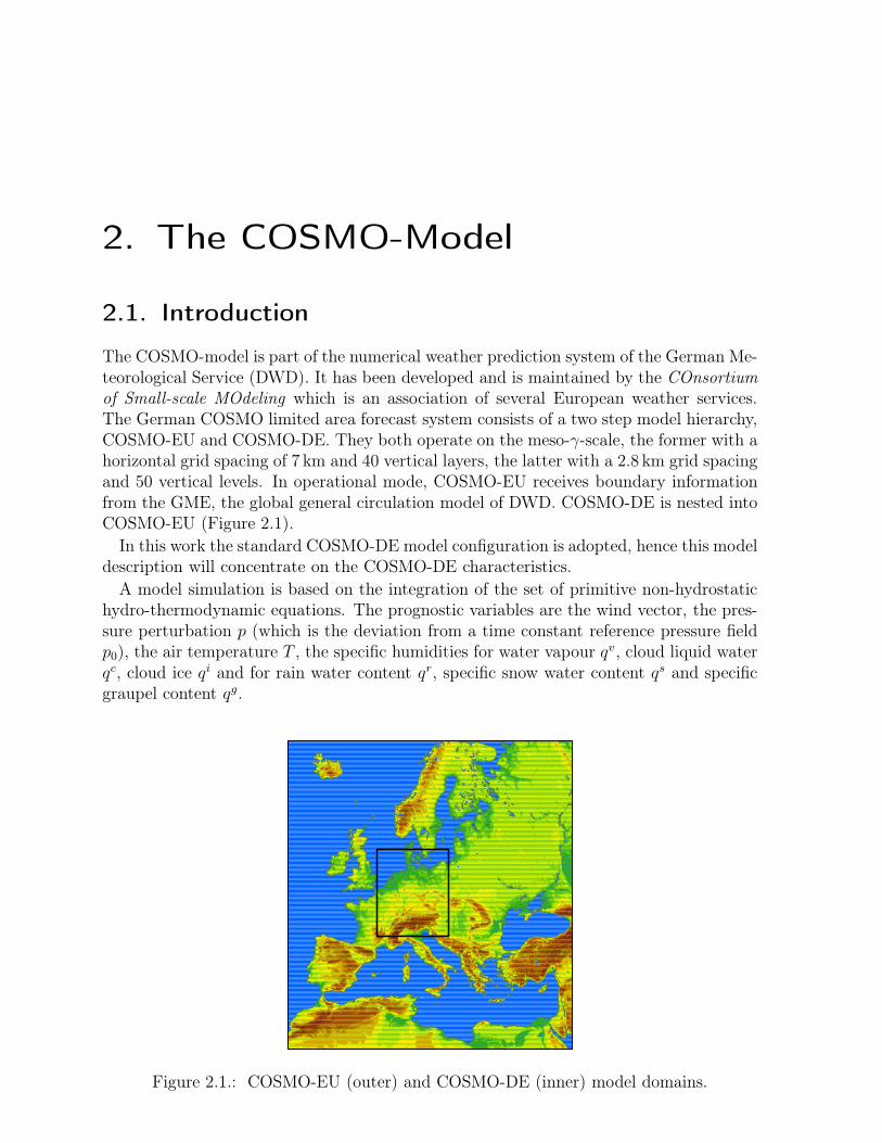
The COSMO-model is part of the numerical weather prediction system of the German Me-teorological Service (DWD). It has been developed and is maintained by the COnsortiumof Small-scale MOdeling which is an association of several European weather services.The German COSMO limited area forecast system consists of a two step model hierarchy,COSMO-EU and COSMO-DE. They both operate on the meso-γ-scale, the former with ahorizontal grid spacing of 7 km and 40 vertical layers, the latter with a 2.8 km grid spacingand 50 vertical levels. In operational mode, COSMO-EU receives boundary informationfrom the GME, the global general circulation model of DWD. COSMO-DE is nested intoCOSMO-EU (Figure 2.1).
In this work the standard COSMO-DE model configuration is adopted, hence this modeldescription will concentrate on the COSMO-DE characteristics.
A model simulation is based on the integration of the set of primitive non-hydrostatichydro-thermodynamic equations. The prognostic variables are the wind vector, the pres-sure perturbation p (which is the deviation from a time constant reference pressure fieldp0), the air temperature T , the specific humidities for water vapour qv, cloud liquid waterqc, cloud ice qi and for rain water content qr, specific snow water content qs and specificgraupel content qg.
Figure 2.1.: COSMO-EU (outer) and COSMO-DE (inner) model domains.
15

16
0
100
200
300
400
500
600
700
800
900
20m51m94m149m216m
297m
390m
497m
617m
752m
902m
1066m
Layer thickness COSMO−DE
Hei
ght [
m]
Figure 2.2.: Heights of lowest 11 model layer boundaries in COSMO-DE.
2.2. Coordinate system and grid structure
In COSMO, a spherical coordinate system is employed with geographical longitudes andlatitudes as horizontal coordinates and the distance from the earth surface as verticalcoordinate. The model grid is based on a rotated coordinate system with the modelequator intersecting the centre of the model domain, to avoid the problem of convergingcoordinate lines towards the pole. The vertical coordinate ζ is a hybrid vertical coordinatewhich is parallel to the orography in the lower levels and horizontal in the upper part.The grid box boundaries are referred to as half-levels in contrast to the main levels, whichintersect the grid box centre. The thickness of the layers decreases from top to bottom,thus, the vertical resolution near the surface is higher than in the upper atmosphere (seeFigure 2.2). The model variables in COSMO are staggered on an Arakawa-C grid, i.e.temperature, pressure and the humidity variables are defined in the centre of the boxes,whereas the velocity components are defined at the respective grid box faces (Schättleret al., 2005). Using this configuration, a more exact representation of the differentialoperators is obtained in contrast to the Arakawa-A grid, where all variables are definedat the same point.
The model can be run in sequential or parallel mode. For parallel mode horizontaldomain decomposition is applied.
As upper boundary condition the ζ = 1/2 level acts as a rigid lid by setting the verticalvelocity to zero. For avoiding a backscatter of waves at the upper boundary, an enhanceddamping is implemented for the upper model layers.
2.3. System of equations
The model is based a complete set of unfiltered primitive equations with the consequencethat processes at each scale have to be considered, including the fast moving sound andgravity waves. To achieve numerical stability, a small time step has to be used, whichis computationally expensive. The mode splitting approach, proposed by Klemp and

Chapter 2. The COSMO-Model 17
Wilhelmson (1978), is chosen to handle this problem: the equations are split up in termsfor the fast sound wave processes, and for the meteorological relevant processes on largertime scales such as advection and the tendencies from the physical parameterizations.The former are solved with a smaller time step than the slow processes (Steppeler et al.,2002). Thus we have
∂ψ
∂t= fψ + sψ (2.1)
where ψ is any prognostic model variable, fψ is the forcing term for the slow modes andsψ is the source term describing sound- and gravity-waves. During the smaller time steps,the fψ-terms are kept constant.
The basic model equations provide a complete set of the relevant state-variables if allterms describing the impact of the subgrid-scale processes are known. These include thestress tensor, the turbulent fluxes of water vapour, liquid water and ice, the phase changes,the precipitation fluxes of rain, snow and graupel, the sensible heat flux and the radiationflux density. All these processes have to be calculated as functions of the model variablesusing the respective parameterizations (see chapter 2.5).
For solving the equations numerically, the spatial and temporal differential operatorsare replaced by the respective finite differences in space and time. In COSMO-DE theintegration is based on a two-time-level Runge-Kutta integration scheme third order intime (Baldauf et al., 2009). Two other optional integration schemes are implemented inthe model, a three-timelevel time-splitting Leapfrog scheme (used for COSMO-EU) anda threedimensional semi-implicit integration scheme.
2.4. Data assimilation
The model runs in this work are forced by COSMO analyses, therefore a brief descriptionof the COSMO data assimilation methods used to produce the analysis is given in thissection.
For operational data assimilation a nudging technique is implemented, which "pulls"the prognostic model variables into the direction of the observed data. For this purposean additional forcing term, a so-called relaxation term, is introduced into the prognosticequations; the development of a variable ψ can thus be written as (Schraff and Hess,2002):
∂
∂tψ(x, t) = Pψ(x, t) +Gψ ·
∑
k(obs)
(Wk · (ψk − ψ(xk, t))). (2.2)
Pψ denotes the dynamics and parameterizations of the model, ψk is the kth observationinfluencing grid point x at time t, xk is the location of the observation and Gψ is aconstant so-called nudging-coefficient and Wk a weight between 0 and 1, determining towhat degree a grid point should be influenced by a given observation.
The characteristic time scale for the relaxation process is determined by the coefficientGψ, such that that the deviation of the model value from the observed value decreasesin about half an hour to 1/e. In practise, the nudging term is kept smaller than thelargest dynamic and physical terms, in order not to disturb the internal equilibrium of themodel. Fields for which the nudging technique is applied, are horizontal wind, potential

18
temperature and relative humidity on all layers and pressure at the lowest model level. Theanalysis increments are hydrostatically balanced thus avoiding direct sources of verticalwind.
Newly implemented is a method for the incorporation of radar precipitation observationsof the DWD radar composite into the COSMO-DE, the so-called latent heat nudging.Temperature increments are determined proportional to the ratio between observed andsimulated values and to the available latent heat in the model. For this procedure therelative humidity is kept constant which leads to a change in specific humidity. As aconsequence, simulated precipitation is adjusted into the direction of the observation(Baldauf et al., 2009).
The assimilation system is completed by an analysis of sea surface temperatures oncea day, and a snow depth analysis every 6 hours. No soil moisture assimilation is carriedout in COSMO-DE. In COSMO-EU, however, an adjustment of soil moisture is appliedsuch that the 2 m-temperatures corresponds well to the observed temperatures. This isdone by minimizing a cost function (Hess, 2001).
2.5. Parameterizations
In the following a short overview of the different parameterizations of the COSMO model isgiven. The radiation scheme, the turbulence parameterization options and the soil moduleTERRA are described in some more detail, because they are of special importance forthis work.
2.5.1. Grid scale clouds and precipitation
Clouds arise from condensation of cloud water by saturation adjustment. The treatmentof grid scale precipitation is based on a Kessler-type 1-moment-bulk approach (Kessler ,1969), which has been expanded to consider five prognostic water categories: water vapourand hydrometeors of cloud water, cloud ice, rain water, snow, and graupel. The particlesof these classes interact through the parameterization of several microphysical processes(Baldauf et al., 2009).
2.5.2. Partial cloudiness
Clouds produced by the grid scale scheme always cover the whole grid box, i.e. the cloudcover is 100%. For radiative transfer calculations and post-processing applications addi-tional knowledge of the subgrid cloudiness is required. Subgrid cloudiness is consideredby means of an empirical function depending on relative humidity, height, and convectiveactivity.
2.5.3. Moist convection
It is assumed that deep convection (showers and thunderstorms) is a grid scale processat the COSMO-DE scale of 2.8 km. Only shallow convection is parameterized by a massflux scheme of Tiedtke (1989) with a closure based on moisture convergence. However,

Chapter 2. The COSMO-Model 19
no convective precipitation is produced by this scheme, because precipitation forming forshallow convection is excluded. In COSMO-EU also deep convection is parameterized bythe Tiedtke-scheme.
2.5.4. Radiation
The radiation scheme in the COSMO models was developed by Ritter and Geleyn (1992)and is based on the one-dimensional δ-two-stream approximation of the radiative transferequation. The spectrum is divided into broad spectral intervals, for which the radiativetransfer calculations are carried out. Absorption, emission and scattering by cloud par-ticles, aerosols and gas molecules is accounted for. For subgrid-scale clouds in a verticalcolumn the maximum-random overlap assumption is applied. The cloud optical propertiesare parameterized based on a fit of the optical properties of eight cloud types followingStephens (1984). Aerosols are given by a constant climatology. Effects of three gases areconsidered: water vapour, carbon dioxide, which has a constant value of 330 ppm, andozone, the temporal variability of which is described by a climatological annual cycle. Theradiation scheme provides net fluxes at the surface in the solar and thermal regime andthree-dimensional heating rates for every vertical layer in a column.
In COSMO-DE radiation computations are carried out every 15 minutes; these calcu-lations are applied to 2x2 columns of averaged atmospheric properties with a correctionfor the local albedo for the solar radiation surface flux and for ground temperature forthe thermal radiation flux (Baldauf et al., 2009). In COSMO-EU, radiation effects arecalculated hourly and fluxes and heating rates are kept constant in between. The solarzenith angle used in the radiation computations is the zenith angle valid for the middleof the interval between two radiation updates.
2.5.5. Subgrid-scale turbulence
Even for high horizontal resolutions on the order of 102 or 103 meters, a parameteriza-tion of subgrid-scale turbulence is required. At small scales, the boundary layer approx-imation of neglecting horizontal turbulent exchange becomes questionable, therefore athree-dimensional approach is recommended for scales below 1 km.
The turbulence parameterization estimates influence of subgrid scale turbulent diffusionon the gridscale variables in the primitive equations. The formulation is based on K-theory, which relates the subgrid-scale flux to the gradient of a variable ψ and a diffusioncoefficient K, in three-dimensional form:
Fψ = −Kψ · ∇ψ. (2.3)
The mixing coefficients Km and Kh for momentum and heat have to be determined inthe parameterization scheme. In COSMO several options for turbulence schemes areimplemented. Two are used for this work:
Prognostic TKE1 scheme: This is the operational scheme developed by M. Raschen-dorfer, which is based on a closure of order 2.5. The exchange coefficients are calculateddepending on the thermal stratification and vertical wind shear (Doms et al., 2007). The
1Turbulent Kinetic Energy

20
Figure 2.3.: Sublayers of the transfer scheme.
scheme has been extended by an additional TKE source term, which avoids the TKEgetting unrealistically close to zero under stable conditions.
LLM2-Scheme: This scheme has been developed in the framework of the LITFASS3-project for the use in a modified model version of the COSMO model on the 100m scale(Herzog et al., 2002). Here the turbulence coefficients are specified by a more simplePrandtl/Kolmogorov approach based on a first-order closure assumption. The coeffi-cients are parameterized based on stability functions depending on a model developed bySmagorinsky (1963) and a length scale which is a function of the grid spacing to take thenumerical resolution into account. Hence the scheme adapts to the chosen resolution. Incontrast to a one-dimensional scheme, the gradients in three-dimensional space are con-sidered. The horizontal turbulent exchange coefficients are simple functions of the verticalcoefficients.
2.5.6. Surface fluxes
The surface flux transfer scheme computes the flux density of model variables at the lowermodel boundary where only turbulent and molecular processes are of importance, i.e. itacts as the interface between surface and atmosphere. The operational COSMO transferscheme is based on the diagnostic TKE equation, which provides the stability functions,employing the vertical gradients of the model variables, which is needed for calculatingthe turbulent length scale. The transfer layer is divided into three sublayers, as depictedin Figure 2.3. The transport resistance (which is proportional to the reciprocal of thetransfer coefficient) is the sum of the three respective resistances. The lowest layer justabove the rigid earth surface is the laminar sublayer. In the laminar sublayer resistancedue to molecular diffusion is a linear function of height. Above the laminar layer upto the height of the roughness length z0, lies the turbulent roughness layer. Here theresistance is an exponential function of height and dependent on roughness elements. Theturbulent Prandtl layer constitutes the upper part of the transfer layer, which covers halfof the lowest atmospheric model layer, with constant vertical turbulent flux densities and
2LITFASS-Lokal-Modell3Lindenberg Inhomogeneous Terrain - Fluxes between Atmosphere and Surface - a long term Study

Chapter 2. The COSMO-Model 21
Figure 2.4.: Processes and structure of the SVAT module TERRA.
is characterized by a stability dependent resistance which is a logarithmic function ofheight.
2.5.7. Soil processes
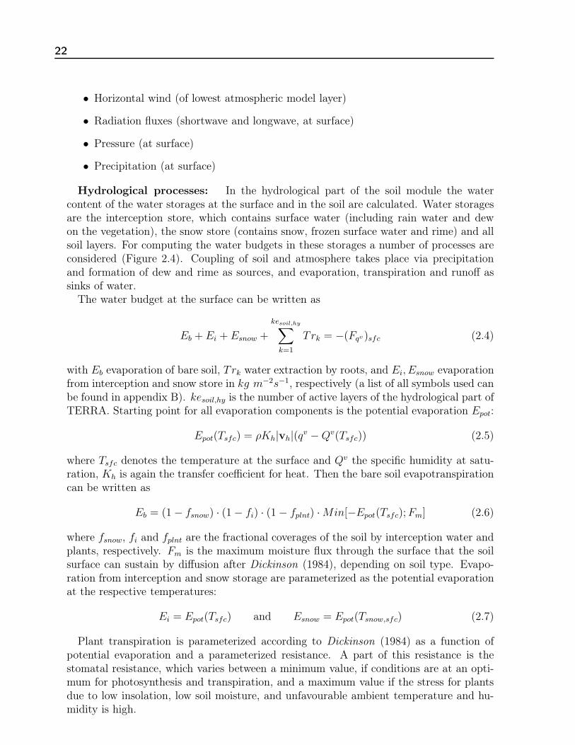
The lower boundary condition is modelled by the soil and vegetation model TERRA(Doms et al., 2007). Two implementations of TERRA are available: the two-layer soilmodel following Jacobsen and Heise (1982) and the extended multi-layer version TERRA-ML.Only the latter option is employed in this work and described in the following.
TERRA calculates the temperature and humidity at the land surface, i.e. at the in-terface between atmosphere and soil. Those quantities are needed for the computationof the surface fluxes of energy and water, which are responsible for the exchange of heat,moisture and momentum between the surface and atmosphere. In TERRA all processesare modeled strictly one-dimensionally, thus no interactions between adjacent soil columnsare considered. An overview of the processes and the structure of TERRA is provided inFigure 2.4.
The atmospheric driving variables for TERRA are:
• Temperature (of lowest atmospheric model layer)
• Humidity (of lowest atmospheric model layer)
22
• Horizontal wind (of lowest atmospheric model layer)
• Radiation fluxes (shortwave and longwave, at surface)
• Pressure (at surface)
• Precipitation (at surface)
Hydrological processes: In the hydrological part of the soil module the watercontent of the water storages at the surface and in the soil are calculated. Water storagesare the interception store, which contains surface water (including rain water and dewon the vegetation), the snow store (contains snow, frozen surface water and rime) and allsoil layers. For computing the water budgets in these storages a number of processes areconsidered (Figure 2.4). Coupling of soil and atmosphere takes place via precipitationand formation of dew and rime as sources, and evaporation, transpiration and runoff assinks of water.
The water budget at the surface can be written as
Eb + Ei + Esnow +
kesoil,hy∑
k=1
Trk = −(Fqv)sfc (2.4)
with Eb evaporation of bare soil, Trk water extraction by roots, and Ei, Esnow evaporationfrom interception and snow store in kg m−2s−1, respectively (a list of all symbols used canbe found in appendix B). kesoil,hy is the number of active layers of the hydrological part ofTERRA. Starting point for all evaporation components is the potential evaporation Epot:
Epot(Tsfc) = ρKh|vh|(qv −Qv(Tsfc)) (2.5)
where Tsfc denotes the temperature at the surface and Qv the specific humidity at satu-ration, Kh is again the transfer coefficient for heat. Then the bare soil evapotranspirationcan be written as
Eb = (1− fsnow) · (1− fi) · (1− fplnt) ·Min[−Epot(Tsfc);Fm] (2.6)
where fsnow, fi and fplnt are the fractional coverages of the soil by interception water andplants, respectively. Fm is the maximum moisture flux through the surface that the soilsurface can sustain by diffusion after Dickinson (1984), depending on soil type. Evapo-ration from interception and snow storage are parameterized as the potential evaporationat the respective temperatures:
Ei = Epot(Tsfc) and Esnow = Epot(Tsnow,sfc) (2.7)
Plant transpiration is parameterized according to Dickinson (1984) as a function ofpotential evaporation and a parameterized resistance. A part of this resistance is thestomatal resistance, which varies between a minimum value, if conditions are at an opti-mum for photosynthesis and transpiration, and a maximum value if the stress for plantsdue to low insolation, low soil moisture, and unfavourable ambient temperature and hu-midity is high.

Chapter 2. The COSMO-Model 23
Thus, after evaluation of Equation 2.4, the surface flux of water vapour is known, andhence the virtual specific humidity qvsfc at the surface can be estimated by a parametricdrag-law formulation:
(Fqv)sfc = −ρKhL|vh|(qv − qvsfc). (2.8)
Here, qv is the specific humidity at the lowest atmospheric layer above the surface, Kh
is the transfer coefficient of heat calculated in the transfer scheme in section 2.5.6, Lis the latent heat of vapourization and |vh| the horizontal wind velocity in the lowestatmospheric layer.
Vertical water transport in the soil occurs due to gravity and capillary forces and isdescribed by the Richards equation:
Fwl= −ρw[−Dw(wl)
∂wl∂z
+Kw(wl)] (2.9)
with Fwlsoil water flux, ρw water density, Dw hydraulic diffusivity and Kw hydraulic
conductivity, which are dependent on water content wl and soil texture. At the upperboundary the flux is replaced by infiltration, which is inherently limited by the maximuminfiltration rate, which is again a function of soil type and wetness of the soil. If thepotential infiltration rate is higher than this limit; the surplus is converted into surfacerunoff and eliminated from the hydrological cycle of the model. Runoff from a soil layeris generated, if the water content of the layer exceeds the field capacity wFC. Soil watercan drain from the lowest soil model layer, but the diffusion flux upwards into layer sixis neglected, i.e. the soil can not be moistened due to moisture gradients by the groundwater. This can lead to dry soils, because the drainage can not be compensated bydiffusion fluxes.
Thermal processes: The basic equation for temperature computations is the heatconduction equation:
∂Tso∂t
=1
(ρc)
∂
∂z(λ∂Tsoil∂z
) (2.10)
with ρc heat capacity and λ heat conductivity. There are seven active layers for heatprocesses, see Figure 2.4. In the eighth layer a constant temperature is assumed, given bythe annual average air temperature at 2 m height above the surface (Baldauf et al., 2009).
At the upper boundary of TERRA the heat flux λ∂T/∂z is replaced by Gsfc, the sumof radiation budget and heat fluxes. This forcing at the surface can be written as
Gsfc = (Fh)sfc + L(Fqv)sfc +Qrad,net +GP +Gsnow,melt (2.11)
consisting of the sum of sensible heat flux (Fh)sfc, latent heat flux L(Fqv)sfc, net radiationQrad,net, which stems from the radiation parameterization, GP which considers effects offreezing rain and melting snowfall, and Gsnow,melt models influence of melting processeson soil temperature. As the energy budget is explicitly used for determining the soil heatflux Gsfc, energy is conserved at the earth surface.
The effective surface temperature TG is an area-weighted average over snow temperatureTsnow and the snow-free temperature surface temperature Tsfc. For water bodies thetemperature is kept constant throughout the model run. For operational use its value isinterpolated from the sea surface temperature (SST) of the nearest sea point. This has

24
been altered for the current work, see section 4.2.External Parameters: An atmospheric model requires information on the state of
the earth’s surface. Two different types of information can be distinguished: primarydata, which are directly extracted from an external data set, and secondary data, whichare transformed primary data. Some of the external data sets are freely available, butsome, such as information on high-resolution soil type, have to be purchased. The primarydata sets are (Doms et al., 2007):
• Orography: For operational applications, the GLOBE data set, which is a DigitalElevation Model (DEM) provided by the National Oceanic and Atmospheric Ad-ministration (NOAA), with a resolution of 30 arc seconds is employed. For derivinginformation on coarser scales, the subgrid elevations are averaged, and the subgrid-scale variance is used for the derivation of the roughness length. Moreover a filteringof steep orography is applied in order to avoid large elevation difference in adjacentgrid boxes in mountainous areas.
• Dominant land cover: Operationally the CORINE (CoORdination of INforma-tion on the Environment) data set, an European initiative with 250 m resolution isused. The vegetation classes in this data set are grouped into more general categorieswith similar characteristics for application in the model.
• Dominant soil type: The data used by DWD are based on the FAO/UNESCOSoil Map of the World from 1974, with a very coarse resolution of 5 arc minutes(∼ 10 km). Hence, the resolution of the data set is more than 3 times coarserthan the COSMO-DE resolution of 2.8 km. For the soil texture eight classes aredistinguished: ’ice’, ’rock’, ’sand’, ’sandy loam’, ’loam’, ’loamy clay’, ’clay’ and’peat’. All thermal and hydraulic parameters (e.g. heat capacity, heat conductivity,field capacity, etc.) are derived from these eight classes by lookup-tables.
• Mean surface temperature is needed for TERRA as constant lower boundarycondition for the deepest soil level, as described above. These data are made avail-able by the University of East Anglia with a 0.5◦ resolution.
Refined new primary data sets have been processed for this work, details are given insection 4.2.
The secondary data sets are determined mainly by lookup-tables:
• Land mask: is primarily determined on the basis of the land cover data. All pixelswhich have a land fraction larger than 50% are treated as land point, otherwise aswater pixel.
• Roughness length: depends on subgrid scale orography and land use, the influenceof the latter one is determined via lookup-tables. Over water surfaces the roughnesslength is not an external parameter but a variable calculated internally as a functionof wind velocity using the Charnock formula.
• Plant cover, leaf area index, rootdepth: These vegetation quantities are notconstant over the year. The maximum and minimum values are determined via

Chapter 2. The COSMO-Model 25
lookup tables from land cover information. The final values are parameterized on thebasis of an interpolation between these maximum and minimum values as functionof Julian day, latitude and elevation.
• Forests: Recently, field masks for deciduous and evergreen forests have been intro-duced to account for the effects of forests on albedo and transpiration.


3. Adaptive radiative transfer
parameterization
3.1. Overview: Radiation codes in numerical weather
prediction models
The increasing resolutions of current weather forecast models of a few kilometres in princi-ple require three-dimensional radiative transfer computations. Accurate radiative transfer(RT) computations based on the three-dimensional spectral radiative transfer equationare, however, extremely complex and computationally demanding. Consequently variousparameterizations, with different degrees of simplifications, have been developed. In par-ticular for the application in operational weather prediction models or for long periodclimate simulations large simplifications are inevitable to reduce computational costs.Common simplifications are the computation of radiative transfer reduced to flux densi-ties on broad spectral bands for one-dimensional vertical atmospheric columns, assuminghorizontal homogeneity within the model column. Also the treatment of clouds in the RTparameterization requires a number of assumptions, e.g. for the overlap of partial cloudcover in the vertical. Many input parameters required for atmospheric radiative transfer,especially cloud characteristics, are highly uncertain and also parameterized in opera-tional models. Despite reductions in complexity, radiation transfer parameterizations arefor most applications still too demanding to be computed for each model timestep andthe full spatial grid. Different approaches have been implemented by the national weatherservices and climate centres to overcome this limitation by sampling in time and space.The most common strategy is temporal sampling, i.e. the radiation scheme is calledat time intervals of more than one model time step. The fluxes and heating rates arekept constant in between, either based on a medium solar zenith angle, or adjusted ineach timestep according to the current solar zenith angle. Spatial sampling strategiesinterpolate between sparse computations or average atmospheric properties over multiplecolumns before passing the data to the RT parameterization.
The Integrated Forecasting System (IFS) of the European Centre for Medium-RangeWeather Forecasts (ECMWF) for example employs a comparatively sophisticated radia-tive transfer scheme since June 2007, making use of the two-stream approximation in theRapid Radiative Transfer Model (RRTM) for shortwave (Clough et al., 2005) and long-wave (Mlawer et al., 1997) radiation, while treating cloud variability by the Monte CarloIndependent Column Approximation (McICA, Pincus et al. (2003)). To save computa-tion time the radiation scheme is called only at large temporal intervals (once per houror once per three hours, depending on model resolution) and on a coarsened grid, wherethe radiative effects are interpolated to the finer grid by a cubic interpolation scheme.The temporal interpolation for each dynamic model timestep is done by accounting for
27

28
the correct solar zenith angle for shortwave flux and for changing surface temperaturesfor the upward longwave flux in each timestep (Morcrette, 2000; Morcrette et al., 2008).
In the COSMO model (Steppeler et al., 2003) also the two-stream approximation isemployed based on code by Ritter and Geleyn (1992); however, as described in section2.5.4 calls to this scheme are also restricted in time and space. The scheme is called eitheronce per forecast hour or quarter-hourly, in the configurations COSMO-EU and COSMO-DE, respectively. In the latter configuration the atmospheric input parameters are firstaveraged over four columns, before carrying out the radiation calculations. The obtainedsurface radiation fluxes are adjusted taking the local albedo and surface temperature intoaccount (Baldauf et al., 2009).
Temporal and spatial sampling methods in radiation transfer code can lead to errors:temporally sampling neglects the varying local insolation due to changes in solar zenithangle and advection and evolution of clouds; spatial averaging reduces spatial variabilityof radiative effects which is problematic due to the nonlinear characteristics of radiativetransfer. Inconsistent situations may occur, when the radiative properties are not allowedto react to the changing atmosphere over several timesteps, thus raining clouds and strongsolar fluxes are allowed to coexist in rapidly changing convective atmospheres. Morcrette(2000) studied the sampling effects on operational simulations and analyses for the IFSglobal model. He found a larger sensitivity with respect to temporal sampling, thanto spatial sampling followed by subsequent interpolation. In 10-day forecasts he foundtemperature errors depending on the temporal frequency of radiation computations. Thiserror increased with height, due to feedbacks between convective clouds and radiation,especially in the tropics. For longer, e.g. seasonal, predictions these errors grow, thus ahigher temporal sampling is beneficial.
Several approaches have been developed in recent years to bypass the conflict betweenthe need of frequent radiation computations and computational limits. Computation timecan be reduced by training an artificial neural network (ANN) with a detailed radiationscheme offline (Chevallier et al., 1998, 2000; Krasnopolski et al., 2005). Krasnopolski et al.(2010) tested such ANNs in the National Center for Environmental Prediction (NCEP)Climate Forecast system (CFS) by comparing simulations with the original inherent ra-diation code (RRTMG) with simulations employing the ANN emulating the complexradiation code. The differences were small and comparable to internal model variability,compiler changes etc. while a considerable speedup was achieved for the climate simula-tions. A drawback of this method is the need to re-train the ANN for any configurationalchanges such as the vertical resolution. Pielke et al. (2005) proposed an approach basedon look-up-tables. Radiative effects for all possible inputs are pre-calculated and storedto disk. As for the ANN, look-up-tables need to be recomputed for every change inthe model setup, making the model inflexible. Furthermore, given the expected increasein the number of model levels, the number of possible combinations may soon becomeprohibitive.
In Venema et al. (2007) (from now on VSAS07) two adaptive radiative transfer parame-terizations are presented, which exploit temporal and spatial correlations in the 3D opticalproperty fields. Radiation calculations by the implemented RT scheme are performed inonly a fraction of time and space. The so-called temporal adaptive scheme identifies thegrid points in the model domain where the largest changes since the last radiation update

Chapter 3. Adaptive radiative transfer parameterization 29
have occurred and targets these columns for the next RT computations. In that way itis guaranteed, that always the grid boxes where the cloud characteristics have changedmost strongly, get an update in radiative effects. These grid cells are chosen employinga simplified radiation scheme, based on multiple linear regression which uses verticallyintegrated atmospheric variables as predictors, estimating the changes in the radiativeeffects since the last update. The rest of the field is updated by computing the change inthe radiative tendencies by the same simplified radiation scheme and adding them to theradiation effects from the last timestep. In the second proposed scheme, the spatial adap-tive scheme, only a small, but fixed part of the field is updated by the internal radiationscheme at high temporal frequency. For the other columns a search for a nearby similaratmospheric column is carried out and the radiative effects of the most similar columnare applied with a correction for solar angle and albedo.
Manners et al. (2009) adopted this idea and developed two adaptive RT schemes inspectral space, and employ a reduced RT calculation at timesteps between calls to the fullcomplex radiation scheme. Their split time-stepping approach divides the RT computationin bands with strong gaseous absorption terms, which are optically thick and hardlydependent on cloud characteristics, and in bands which are optically thin, where cloudshave a strong influence. The latter RT calculations are updated with a higher temporalfrequency to keep track of changes due to developing and advecting clouds. Their secondmethod, the incremental time-stepping method, uses a simple radiation scheme to computetemporal changes for the window region, i.e. the optically thin part of the atmosphericspectrum, where variability is mainly caused by variations in cloud properties. Theseincrements are added to the results of the full complex scheme, which is computed at alower temporal frequency.
The adaptive schemes in VSAS07 were introduced and, as a proof of principle, tested inan offline environment and only for the radiative net fluxes at the surface. In a case study itwas shown that such schemes are able to predict the surface fluxes much more accurately,using the same computational resources as used for the standard temporal and spatialsampling methods. In addition, the spatial error fields of the adaptive approaches werecharacterized by notably smaller correlation lengths. The reduction in the number of callsto the complex scheme leads to only a small reduction in accuracy. The spatial adaptivescheme gave overall better results than the temporal adaptive scheme. Therefore, in thiswork results from the implementation of the spatial scheme in the operational weatherforecast model COSMO are presented. The spatial adaptive radiation parameterizationhas been extended to be applied also to the vertical heating rates. The performance of thisenhanced scheme is compared to the standard operational radiation update scheme. Inthe next section, the adaptive scheme is introduced, whereas in section 3.3 the performedsimulations and experiments are outlined. Section 3.4 contains the results of the adaptivescheme as applied in the COSMO model, these results are discussed in section 3.5. Thischapter on the adaptive radiation scheme has been published in Schomburg et al. (2011).
3.2. Enhanced adaptive radiation scheme
VSAS07 presented two adaptive radiative transfer schemes, termed temporal and spatialadaptive scheme, respectively. Both schemes apply so-called intrinsic calculations, i.e.

30
Table 3.1.: Cost function for finding a nearby radiatively similar atmospheric column. Theweights are optimized for minimal heating rate errors.
Cost function δ = w1∆CCL+w2∆CCT +w3∆LLWP +w4∆IWV +w5∆α+w6∆t+w7dist
Weights w1 = 0.37; w2 = 7.85; w3 = 2.1734 (kgm−2)−1; w4 = 2.0801 (kgm−2)−1;w5 = 13.69; w6 = 0.0018s−1; w7 = 0.744;
CCL: low level clouds (below 800 hPa) [1]; CCT : total cloud cover [1]; LLWP : logarithm of liquid
water path [kg m−2]; IWV : integrated water vapour [kg m−2]; α: surface albedo [1]; t: time since last
update [s]; dist: distance between grid points [1].
calculations made by the atmospheric models own complex radiation scheme, and extrinsiccalculations, which apply a simple generalization algorithm to the intrinsic calculations forgrid points not updated by a call to the complex scheme. The number of intrinsic radiationcomputations is kept comparable to that for the operational configuration, but distributedin a more efficient way. This work is restricted to the spatial adaptive scheme, because itgave overall better results according to VSAS07, i.e. the correlation in the fields could beexploited more efficiently with the spatial scheme than with the temporal scheme. In thiswork the scheme has been extended to atmospheric heating rates and some further smallimprovements have been introduced. Furthermore, the scheme has been implemented andtested in the COSMO model for investigating impacts for numerical weather forecasts onthe meso-γ scale.
The spatial search scheme exploits spatial correlations in the radiative effects in thefollowing way: Only in the first timestep of the model simulation the radiation routine iscalled once for the whole field. For all following timesteps, the model domain is dividedinto small subdomains. At a high frequency the radiation effects at only one of thesubdomain columns is updated by a call to the intrinsic radiation scheme. For gridpoints not updated a search is performed for a nearby similar, recently updated column.Similarity is evaluated by comparing a weighted sum of absolute differences in low cloudcover, total cloud cover, liquid water path, integrated water vapour, surface albedo, timesince the last update of the respective column and distance between the two columns (seeTable 3.1). This weighted search sum has been extended by the spatial distance betweenthe columns and the integrated water vapour compared to the version introduced inVSAS07. Having found the most similar column, the shortwave (SW), longwave (LW) andphotosynthetic active radiation (PAR) surface fluxes and atmospheric heating rate profilesare copied to the respective column. The solar fluxes and heating rates are corrected forsolar zenith angle, and the surface fluxes also for the local albedo. For the longwavesurface fluxes a correction, according to the local surface temperature, has been applied(see Table 3.2).
3.3. Implementation and experimental design
The adaptive scheme is compared with the operational radiation configuration of COSMO-DE, i.e. with radiation calculations carried out for 2x2 averaged columns every 15 minutes.For clarity of notation the scheme will be referred to as “2x2” scheme from now on. The

Chapter 3. Adaptive radiative transfer parameterization 31
Table 3.2.: Adjustment of radiation effects after coping a nearby, recently updated columnin the adaptive scheme.
Variable Correction
Column of SW heating rate HSW = HSWcos(Θx)cos(Θc)
SW and PAR surface radiation flux FSW/PAR = FSW/PARcos(Θx)cos(Θc)
1−αx
1−αc
Column of LW heating rate no correctionLW surface radiation flux FLW = FLW + (σ(1− αIR)(T
4G,c − T 4
G,x)
Θ: solar zenith angle, α: surface albedo, σ: Stefan Boltzmann constant, TG: ground temperature, αIR:infrared albedo; the indices c and x denote the value from the copied and the actual local grid point,respectively.
Table 3.3.: Overview of radiation configurations.
Radiation scheme Call frequency [min] Number of columns updated
Reference 2.5 allAdaptive 2.5 1/25COSMO-DE (2x2) 15 1/4 (averaging 2x2 columns)
adaptive scheme is called every 2.5 minutes, applying the intrinsic radiation scheme onlyfor one out of 5x5 atmospheric columns, while the extrinsic generalization is applied tothe other columns (see Fig. 3.1). This setup requires about the same computation timeas the standard COSMO-DE setup. Update patterns for the adaptive approach, i.e. thesequence in which the pixels are updated, are given in VSAS07 for regions of different size:the ordering is such that subsequently updated columns have a large distance betweenthem.
The most accurate results with respect to radiation would be obtained by radiationcomputations for the full domain on a high temporal frequency. This optimal but muchtoo expensive setup has been taken as reference for testing our adaptive scheme andthe standard COSMO-DE 2x2 configuration. Unless denoted otherwise, all comparisonsshown in the following are based on intrinsic radiation computations carried out every 2.5minutes on the full model domain. The radiation configurations compared are listed inTable 3.3.
For the comparisons a COSMO model version was developed in which the differentradiation options are computed diagnostically, i.e. the dynamics are driven by one of thethree radiation options, which is for most comparisons the reference setup. The radiationeffects of the other two schemes are computed in addition and provided as additionalmodel output.
The largest errors of radiation effects are expected for situations with heterogeneousatmospheric conditions, i.e. small-scale convective cloud patterns, where the atmosphericstate changes rapidly and hence frequent radiation calculations are most important. Threedays have been chosen for the comparison, which span a range from mainly convective tomore stratiform clouds. The first day is a convective summer day, 21 June 2004, wheninstable air masses covered Central Europe under an elevated trough, and a large number
32
´
2
3
46
7
8
9
10
11
13
14
16
17
18
19
20
21
22
23
24
1
2
3
4
5
6
7
8
9
10
11
12
13
14
15
16
17
18
19
20
21
23
24
25
2
3
46
7
8
9
10
11
13
14
16
17
18
19
20
21
22
23
24
1
5
12
15
25
1
5
12
15
25
1
2
3
4
5
6
7
8
9
10
11
12
13
14
15
16
17
18
19
20
21
22
23
24
25
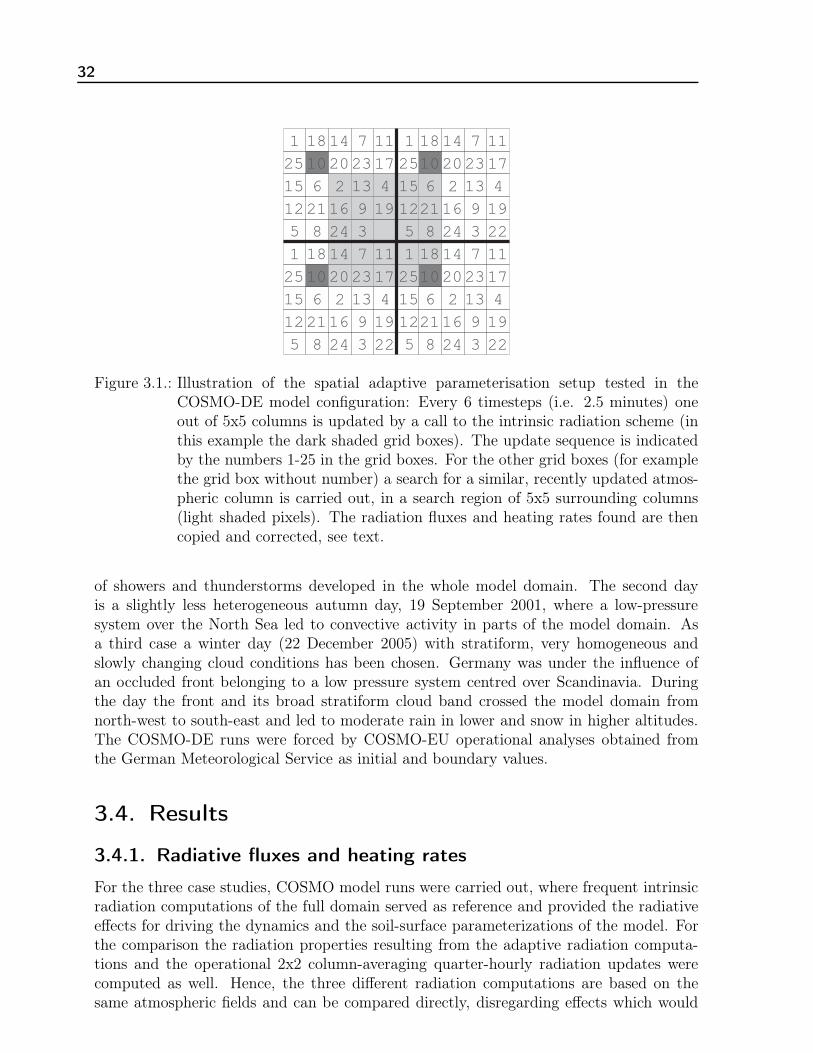
Figure 3.1.: Illustration of the spatial adaptive parameterisation setup tested in theCOSMO-DE model configuration: Every 6 timesteps (i.e. 2.5 minutes) oneout of 5x5 columns is updated by a call to the intrinsic radiation scheme (inthis example the dark shaded grid boxes). The update sequence is indicatedby the numbers 1-25 in the grid boxes. For the other grid boxes (for examplethe grid box without number) a search for a similar, recently updated atmos-pheric column is carried out, in a search region of 5x5 surrounding columns(light shaded pixels). The radiation fluxes and heating rates found are thencopied and corrected, see text.
of showers and thunderstorms developed in the whole model domain. The second dayis a slightly less heterogeneous autumn day, 19 September 2001, where a low-pressuresystem over the North Sea led to convective activity in parts of the model domain. Asa third case a winter day (22 December 2005) with stratiform, very homogeneous andslowly changing cloud conditions has been chosen. Germany was under the influence ofan occluded front belonging to a low pressure system centred over Scandinavia. Duringthe day the front and its broad stratiform cloud band crossed the model domain fromnorth-west to south-east and led to moderate rain in lower and snow in higher altitudes.The COSMO-DE runs were forced by COSMO-EU operational analyses obtained fromthe German Meteorological Service as initial and boundary values.
3.4. Results
3.4.1. Radiative fluxes and heating rates
For the three case studies, COSMO model runs were carried out, where frequent intrinsicradiation computations of the full domain served as reference and provided the radiativeeffects for driving the dynamics and the soil-surface parameterizations of the model. Forthe comparison the radiation properties resulting from the adaptive radiation computa-tions and the operational 2x2 column-averaging quarter-hourly radiation updates werecomputed as well. Hence, the three different radiation computations are based on thesame atmospheric fields and can be compared directly, disregarding effects which would

Chapter 3. Adaptive radiative transfer parameterization 33
Table 3.4.: Daily mean root mean square differences and systematic deviations (bias) fromthe reference simulation for shortwave and longwave surface net fluxes.
RMSD [W m−2] Bias [W m−2]
Day SW LW SW LW2x2 adapt 2x2 adapt 2x2 adapt 2x2 adapt
21-06-2004 31.43 23.80 7.15 5.34 -2.01 -0.20 -0.09 0.0719-09-2001 19.62 15.81 6.53 5.08 -0.60 -0.17 -0.05 0.0822-12-2005 2.36 1.71 5.25 4.14 -0.08 -0.04 0.11 0.07
result from diverging dynamics in different model runs. The resulting radiative fluxes andheating rates were written to an output file every 2.5 minutes.
The adaptive scheme reduces the hourly averaged RMSD for the summer case by about25% in both the shortwave and longwave regime; also the bias is largely decreased, seeFigure 3.2. The instantaneous (2.5min) errors of the COSMO-DE radiation scheme showa quarter-hourly cycle due to the 15-minute update cycle. Errors are low directly aftera new computation of the full field and increase during the following 15 minutes. Theinstantaneous errors of the adaptive scheme are lower throughout the time. The errors ofthe COSMO-DE fluxes do not reach zero at a new calculation at a quarterly hour intervalbecause of two reasons: Firstly, the solar zenith angle is taken as at the middle of theupdate interval, which leads to deviations from the reference values, and secondly errorsarise due to the averaging over four columns.
The root mean square errors and biases for the surface fluxes for all three cases are listedin Table 3.4. The adaptive scheme almost always outperforms the 2x2 standard scheme.The errors are generally smaller for the more homogeneous cases, but about the samerelative improvement compared to the 2x2 scheme is achieved by the adaptive scheme asfor the summer day.
The daily cycle of the errors for the atmospheric heating rates is depicted in Figure 3.3.The RMSD for the shortwave heating rates hardly differ between the adaptive and the2x2 scheme, whereas in the longwave regime the adaptive scheme has the higher RMSD.The systematic errors are small, but the adaptive scheme clearly outperforms the 2x2scheme (lower panel in Fig. 3.3). Only during sunset the solar radiation shows highsystematic errors, probably due to the fast changing path lengths of the sun throughthe atmosphere leading to very different transmissivities. The average vertical profile ofRMSD and bias (see Figure 3.4) shows that the adaptive scheme leads to larger randomerrors for the cloud level, while the systematic errors are much smaller, especially the LWbias. This behaviour can be traced to the weighted difference function used to searchfor the most similar column, which is mainly based on vertically integrated atmosphericproperties. Hence columns of heating rates may be copied which have the same integratedcloud properties, but differ in the vertical position of the clouds. Such errors are penalizedtwice in the root mean square difference, once in the level where radiation is overestimatedand once in the level where it is underestimated. The systematic errors over the wholefield, however, are small. In the 2x2 operational COSMO-DE radiation scheme systematicerrors can occur due to the averaging of the atmospheric properties, which can lead tobiases due to the nonlinearity of radiative transfer processes, especially in case of clouds.

34
5 10 15 200
20
40
60
80
100
120H
ourly
mea
n R
MS
D S
W, [
W m
−2 ]
Hours (UTC)5 10 15 20
0
2
4
6
8
10
12
14
Hou
rly m
ean
RM
SD
LW
, [W
m−
2 ]
Hours (UTC)
5 10 15 20−20
−15
−10
−5
0
5
10
15
Hou
rly m
ean
bias
SW
, [W
m−
2 ]
Hours (UTC)5 10 15 20
−1.5
−1
−0.5
0
0.5
1
Hou
rly m
ean
bias
LW
, [W
m−
2 ]
Hours (UTC)
2x2; 15min (inst)adaptive (inst)2x2; 15min (hourly avg)adaptive (hourly avg)
Figure 3.2.: Top: Instantaneous and hourly averaged root mean square differences in sur-face net radiation fluxes for shortwave (left) and longwave (right) for the 2x2COSMO-DE scheme (solid) and for the adaptive scheme (dashed), for 21June 2004. Bottom: The same for the biases. For the adaptive scheme theinstantaneous and hourly averaged errors are almost identical.
Table 3.5 summarizes the daily mean values of the heating rate errors for the threecase studies. Averaged over the day, the COSMO-DE radiation scheme performs betterthan the adaptive scheme for the longwave RMSD. The average bias over the day issmall, although instantaneous biases can be much larger. The reason is the shape ofthe diurnal cycle of the bias, which shows an overestimation (underestimation) for theshortwave (longwave) heating rates in the morning and vice versa in the afternoon for allcase studies, averaging to a small value close to zero over the day. The hourly biases ofthe 2x2 scheme are almost always higher than for the adaptive scheme (Fig. 3.3 bottom).
An interesting characteristic of the error fields is the temporal autocorrelation, i.e.the correlation of the errors with time lag. Buizza et al. (1999) showed that temporallypersistent perturbations have a remarkable influence on model dynamic development (intheir study model runs with temporally correlated perturbations increased the divergenceof the model runs in an ensemble), while noise which varies randomly from timestep totimestep has no considerable influence. In this study the temporal correlations of thedifference fields could be reduced by about 34% and 45% for the shortwave and longwavesurface fluxes, respectively. The spatial autocorrelations of the difference fields have also

Chapter 3. Adaptive radiative transfer parameterization 35
5 10 15 200
0.005
0.01
0.015
0.02
0.025
Hou
rly m
ean
RM
SD
SW
[K h
−1 ]
Hours (UTC)
2x2; 15minadaptive
5 10 15 200.015
0.02
0.025
0.03
0.035
0.04
0.045
Hou
rly m
ean
RM
SD
LW
[K h
−1 ]
Hours (UTC)
5 10 15 20−6
−4
−2
0
2
4
6x 10
−4
Hou
rly m
ean
bias
SW
[K h
−1 ]
Hours (UTC)5 10 15 20
−2
−1
0
1
2
3
4x 10
−4
Hou
rly m
ean
bias
LW
[K h
−1 ]
Hours (UTC)
Figure 3.3.: Diurnal cycle of mean root mean square differences and bias for columns ofatmospheric heating rates for the summer case 21 June 2004. Left: shortwave;right: longwave.
−1 −0.5 0 0.5 1
x 10−3
0
0.5
1
1.5
2x 10
4
Mean bias SW [K h−1]
Hei
ght [
m]
−4 −2 0 2 4
x 10−3
0
0.5
1
1.5
2x 10
4
Mean bias LW [K h−1]
Hei
ght [
m]
0 0.01 0.02 0.030
0.5
1
1.5
2x 10
4
Mean RMSD SW [K h−1]
Hei
ght [
m]
2x2; 15minadaptive
0 0.02 0.04 0.06 0.08 0.10
0.5
1
1.5
2x 10
4
Mean RMSD LW [K h−1]
Hei
ght [
m]
Figure 3.4.: Mean profile of root mean square differences and bias of atmospheric heatingrates for the summer case 21 June 2004. Left: shortwave, Right: longwave.
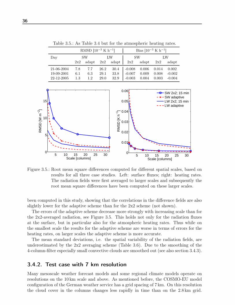
36
Table 3.5.: As Table 3.4 but for the atmospheric heating rates.
RMSD [10−3 K h−1] Bias [10−3 K h−1]
Day SW LW SW LW2x2 adapt 2x2 adapt 2x2 adapt 2x2 adapt
21-06-2004 7.8 7.7 26.2 30.4 -0.008 0.006 0.014 0.00219-09-2001 6.1 6.3 29.1 33.8 -0.007 0.009 0.008 -0.00222-12-2005 1.3 1.2 29.0 32.9 -0.003 0.004 0.003 -0.004
5 10 15 20 25 300
5
10
15
Scale [columns]
RM
SD
[W m
−2 ]
5 10 15 20 25 300
0.01
0.02
0.03
0.04
0.05
0.06
Scale [columns]
RM
SD
[K h
−1 ]
SW 2x2; 15 minSW adaptiveLW 2x2; 15 minLW adaptive
Figure 3.5.: Root mean square differences computed for different spatial scales, based onresults for all three case studies. Left: surface fluxes; right: heating rates.The radiation fields were first averaged to larger scales and subsequently theroot mean square differences have been computed on these larger scales.
been computed in this study, showing that the correlations in the difference fields are alsoslightly lower for the adaptive scheme than for the 2x2 scheme (not shown).
The errors of the adaptive scheme decrease more strongly with increasing scale than forthe 2x2-averaged radiation, see Figure 3.5. This holds not only for the radiation fluxesat the surface, but in particular also for the atmospheric heating rates. Thus while onthe smallest scale the results for the adaptive scheme are worse in terms of errors for theheating rates, on larger scales the adaptive scheme is more accurate.
The mean standard deviations, i.e. the spatial variability of the radiation fields, areunderestimated by the 2x2 averaging scheme (Table 3.6). Due to the smoothing of the4-column-filter especially small convective clouds are smoothed out (see also section 3.4.3).
3.4.2. Test case with 7 km resolution
Many mesoscale weather forecast models and some regional climate models operate onresolutions on the 10 km scale and above. As mentioned before, the COSMO-EU modelconfiguration of the German weather service has a grid spacing of 7 km. On this resolutionthe cloud cover in the columns changes less rapidly in time than on the 2.8 km grid.
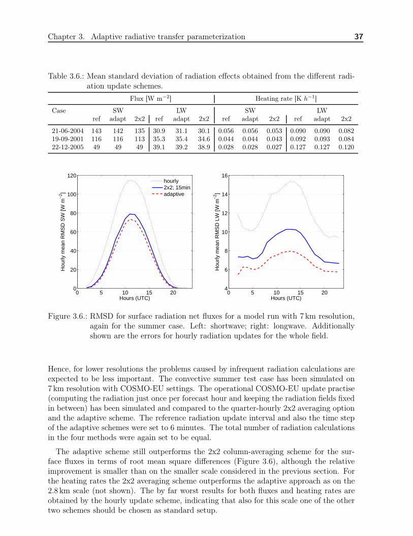
Chapter 3. Adaptive radiative transfer parameterization 37
Table 3.6.: Mean standard deviation of radiation effects obtained from the different radi-ation update schemes.
Flux [W m−2] Heating rate [K h−1]
Case SW LW SW LWref adapt 2x2 ref adapt 2x2 ref adapt 2x2 ref adapt 2x2
21-06-2004 143 142 135 30.9 31.1 30.1 0.056 0.056 0.053 0.090 0.090 0.08219-09-2001 116 116 113 35.3 35.4 34.6 0.044 0.044 0.043 0.092 0.093 0.08422-12-2005 49 49 49 39.1 39.2 38.9 0.028 0.028 0.027 0.127 0.127 0.120
0 5 10 15 200
20
40
60
80
100
120
Hours (UTC)
Hou
rly m
ean
RM
SD
SW
[W m
−2 ]
hourly2x2; 15minadaptive
0 5 10 15 204
6
8
10
12
14
16
Hours (UTC)
Hou
rly m
ean
RM
SD
LW
[W m
−2 ]
Figure 3.6.: RMSD for surface radiation net fluxes for a model run with 7 km resolution,again for the summer case. Left: shortwave; right: longwave. Additionallyshown are the errors for hourly radiation updates for the whole field.
Hence, for lower resolutions the problems caused by infrequent radiation calculations areexpected to be less important. The convective summer test case has been simulated on7 km resolution with COSMO-EU settings. The operational COSMO-EU update practise(computing the radiation just once per forecast hour and keeping the radiation fields fixedin between) has been simulated and compared to the quarter-hourly 2x2 averaging optionand the adaptive scheme. The reference radiation update interval and also the time stepof the adaptive schemes were set to 6 minutes. The total number of radiation calculationsin the four methods were again set to be equal.
The adaptive scheme still outperforms the 2x2 column-averaging scheme for the sur-face fluxes in terms of root mean square differences (Figure 3.6), although the relativeimprovement is smaller than on the smaller scale considered in the previous section. Forthe heating rates the 2x2 averaging scheme outperforms the adaptive approach as on the2.8 km scale (not shown). The by far worst results for both fluxes and heating rates areobtained by the hourly update scheme, indicating that also for this scale one of the othertwo schemes should be chosen as standard setup.

38
0 0.5 1 1.5 20
50
100
150
200
250
LWP [kg m−2]
Sol
ar s
urfa
ce n
et fl
ux [W
m−
2 ]
reference2x2; 15 minadaptive
0 0.5 1 1.5 2−40
−35
−30
−25
−20
−15
Infr
ared
sur
face
net
flux
[W m
−2 ]
LWP [kg m−2]
0 100 200 300 400 5000
0.005
0.01
0.015
0.02
Pro
babi
lity
dens
ity e
stim
ate
Solar flux [W m−2]
LWP=0.5 kg m−2
−100 −50 0 500
0.01
0.02
0.03
0.04
0.05
0.06
0.07
Pro
babi
lity
dens
ity e
stim
ate
Infrared flux [W m−2]
LWP=0.5 kg m−2
Figure 3.7.: Top: Mean shortwave (left) and longwave (right) surface net fluxes for differ-ent LWP values. For legability cloudfree columns have been omitted. Bottom:Estimated probability density function of radiation fluxes for a LWP value of0.5 kg m−2, based on a normal kernel function. Data taken from 1200 to 1700UTC on 21 June 2004.
3.4.3. Physical consistency
In addition to the quantitative performance in terms of errors of the radiation fields alsoconsistency of radiative effects within the model with other variables and other physicalparameterizations is of importance. To illustrate physical relations between radiativeeffects and cloud characteristics, the mean solar and infrared surface fluxes as a function ofthe atmospheric liquid water content are depicted in Figure 3.7 (top). For increasing liquidwater path (LWP) the solar (infrared) surface net flux decreases (increases) logarithmicallyfor the reference and the adaptive radiation, whereas for the 2x2 averaging scheme thisbehaviour is less pronounced. Also the probability density function for a specific LWPvalue (Figure 3.7, bottom) is much wider, less peaked and shifted to higher values for the2x2 scheme, illustrating that too high radiation fluxes may occur for thick clouds; thisdistinction is most pronounced for the shortwave flux (Fig. 3.7 lower left panel). Againthis relation is much better captured by the adaptive scheme.
To study the physical consistency more quantitatively one could compute this probabil-ity density function for each LWP value, yielding a 2D histogram of LWP and solar surface

Chapter 3. Adaptive radiative transfer parameterization 39
5 10 15 200
0.5
1
1.5
2
2.5
Time [h] UTC
RM
SD
2D
EC
DF
x 1
00
5 10 15 200
0.1
0.2
0.3
0.4
0.5
Time [h] UTCR
MS
D 2
D E
CD
F x
100
SW 2x2; 15 minSW adaptiveLW 2x2; 15 minLW adaptive
Figure 3.8.: Left: RMS difference between the ECDFs for logarithmic LWP (left) and rainrate (right) and surface radiation fluxes of the 2x2-column-averaging schemeand the adaptive scheme for the summer case study. The light grey barsdenote sunrise and sunset, respectively. Right: The same for rain rates andradiation fluxes.
net flux and subsequently calculate the RMSD between this histogram for the referenceradiation and one of the other schemes. The disadvantage of a histogram is, however,that the RMSD can depend on the bins widths chosen. Therefore, this error measurehas been computed on the 2D empirical cumulative distribution functions (ECDF). Thetwo-dimensional ECDF is obtained from a two-dimensional histogram by integrating inboth directions. In this way, small random errors do not have a strong influence, butsystematic deviations do.
In Figure 3.8 the root mean square differences of these ECDFs with respect to the ECDFof the reference radiation are depicted, for LWP and surface radiation net fluxes (left) andrain rate and surface net fluxes (right), respectively. Evidently, the differences betweenthe 2x2-column averaging scheme and the reference is much larger, both for shortwaveand longwave net fluxes, than for the adaptive scheme. This illustrates that the radiativevariables computed by the adaptive radiation scheme are much more consistent withother model variables; as expected. For the 2x2 scheme the LW errors show a peak duringthe first hours of the model run; this peak is even more pronounced in the other two casestudies (not shown). This can be explained by a spin-up effect, caused by the initializationwith coarser scale analysis (7 km grid spacing). In the first hour of the model simulationthe cloud cover changes rapidly, from the smooth coarse scale cloud field to a cloud fieldrealistic for this scale. Thus, especially in the first hour an appropriate sampling of theradiative effects is important.
3.4.4. Effects on model dynamics
For the evaluation of different radiation parameterizations the overall effect on the modeldynamics is very important. It is desirable that the errors inevitably caused by any ra-diation scheme, which samples in time and space, has negligible influence on the model

40
5 10 15 200
0.5
1
1.5x 10
−3N
orm
alis
ed R
MS
D s
urfa
ce p
ress
ure
[1]
Hours (UTC)
adaptive2x2; 15 min
5 10 15 200
0.05
0.1
0.15
0.2
0.25
0.3
0.35
0.4
0.45
Nor
mal
ised
RM
SD
tota
l pre
cipi
tatio
n [1
]
Hours (UTC)5 10 15 20
0
0.02
0.04
0.06
0.08
0.1
0.12
0.14
Nor
mal
ised
RM
SD
T2m
[1]
Hours (UTC)
Figure 3.9.: Root mean square difference of surface pressure, total precipitation and 2mtemperature for model runs driven by different radiative forcing for 21 June2004. The errors are normalized with the standard deviations of the referencefield for the respective variable.
dynamics, i.e. the weather development. To investigate this effect, three single model runshave been carried out, one driven by the high-frequent reference radiation computations,one driven by the adaptive radiation computations and one with the quarter-hourly 2x2averaging COSMO-DE scheme. For a numerical weather forecast model it is highly rel-evant how much the two computationally cheaper model runs diverge from the referencemodel run. In Figure 3.9 the RMS difference for three variables, which are importantin daily weather forecasts and good indicators of the dynamical behaviour of the model,is displayed (for the summer case). These are the surface pressure, the total precipita-tion (sum since model initialization) and 2m temperature, normalized with the standarddeviations of the respective reference field to remove effects which are caused by the di-urnal cycle alone. The differences in total precipitation and 2m temperature are causedby differences in cloud formation and movement. The root mean squared differences arelarger for the 2x2 radiation update configuration for all three variables, indicating thatthe model run with the adaptive radiation diverges less. These dynamical effects havebeen verified for a second convective day to ensure robustness of the results (Fig. 3.10).
3.5. Summary and discussion
The concept of adaptive parameterizations for radiative surface fluxes had been intro-duced first in VSAS07. Now, in this work, the spatial adaptive scheme has been improvedand extended to heating rate profiles. The scheme has been implemented and tested inthe COSMO-DE model with the same setup as used for daily weather forecast simula-tions by the German meteorological service on 2.8 km horizontal resolution. The resultsfor case studies with different synoptic conditions were compared with radiative effectscomputed with the standard radiation setup based on four (2x2) averaged columns com-
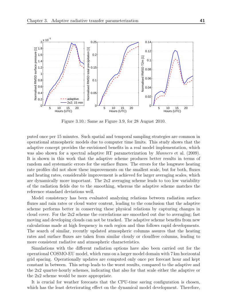
Chapter 3. Adaptive radiative transfer parameterization 41
5 10 15 200
0.2
0.4
0.6
0.8
1
1.2
1.4
1.6
1.8
2x 10
−3N
orm
alis
ed R
MS
D s
urfa
ce p
ress
ure
[1]
Hours (UTC)
adaptive2x2; 15 min
5 10 15 200
0.05
0.1
0.15
0.2
0.25
Nor
mal
ised
RM
SD
tota
l pre
cipi
tatio
n [1
]
Hours (UTC)5 10 15 20
0
0.02
0.04
0.06
0.08
0.1
0.12
0.14
Nor
mal
ised
RM
SD
T2m
[1]
Hours (UTC)
Figure 3.10.: Same as Figure 3.9, for 28 August 2010.
puted once per 15 minutes. Such spatial and temporal sampling strategies are common inoperational atmospheric models due to computer time limits. This study shows that theadaptive concept provides the envisioned benefits in a real model implementation, whichwas also shown for a spectral adaptive RT parameterization by Manners et al. (2009).It is shown in this work that the adaptive scheme produces better results in terms ofrandom and systematic errors for the surface fluxes. The errors for the longwave heatingrate profiles did not show these improvements on the smallest scale, but for both, fluxesand heating rates, considerable improvement is achieved for larger averaging scales, whichare dynamically more important. The 2x2 averaging scheme leads to too low variabilityof the radiation fields due to the smoothing, whereas the adaptive scheme matches thereference standard deviations well.
Model consistency has been evaluated analyzing relations between radiation surfacefluxes and rain rates or cloud water content, leading to the conclusion that the adaptivescheme performs better in conserving these physical relations by capturing changes incloud cover. For the 2x2 scheme the correlations are smoothed out due to averaging; fastmoving and developing clouds can not be tracked. The adaptive scheme benefits from newcalculations made at high frequency in each region and thus follows rapid developments.The search of similar, recently updated atmospheric columns assures that the heatingrates and surface fluxes are taken from similar cloudy or cloudfree columns, leading tomore consistent radiative and atmospheric characteristics.
Simulations with the different radiation options have also been carried out for theoperational COSMO-EU model, which runs on a larger model domain with 7 km horizontalgrid spacing. Operationally updates are computed only once per forecast hour and keptconstant in between. This setup leads to the worst results, compared to the adaptive andthe 2x2 quarter-hourly schemes, indicating that also for that scale either the adaptive orthe 2x2 scheme would be more appropriate.
It is crucial for weather forecasts that the CPU-time saving configuration is chosen,which has the least deteriorating effect on the dynamical model development. Therefore,

42
single model runs were carried out where the different radiation quantities of the adaptiveand 2x2 averaging schemes were not just computed diagnostically, but were actively usedto force the model. We found that the model runs with the operational quarter-hourly2x2 averaged radiation diverges more from the reference model run with highly frequentcalls to radiation scheme than the model run employing the adaptive scheme. Thus, itcan be concluded, that the lower errors for the surface fluxes, the better performance forthe heating rates on larger averaging scales, and the more realistically captured physicalrelations have a highly positive impact. All this is achieved without an increase in compu-tation time, but based on a more intelligent way of exploiting the available computationresources, and distributing the information from the complex radiation scheme to the restof the field.
For training the scheme an optimization algorithm had to be applied to find the weightsfor the cost function used to search for nearby similar columns. In VSAS07 it was shown,that the scheme is not sensitive to the exact values of these weights. Hence an advantagecompared to neural networks, which emulate complex radiation schemes (e.g. Krasnopolskiet al., 2010) is that re-training is much less important for changes in the radiation schemeor the vertical resolution, the scheme can be applied as-is in other atmospheric models orin combination with other radiation codes. The obtained speedup, however, is potentiallysmaller than for neural networks because the complex radiation scheme is not emulatedbut only exploited more efficiently. If a neural network is employed for the radiativetransfer, no online radiation computation with the complex radiation scheme are carriedout at all.
As further improvement of the scheme a combination of the spatial adaptive schemewith the temporal adaptive scheme proposed in VSAS07 is planned. In that scheme thegrid points for which a call to the complex radiation scheme is carried out are not fixed(see section 3.1), but a very simple radiation scheme based on a multiple linear regressionis used to find the columns that have undergone the largest atmospheric changes since thelast update. This gives even better information on the radiative quantities in regions wherethe clouds are developing and moving rapidly. Furthermore, remaining differences betweenthe best matching nearby column and the true atmospheric profile can be corrected bythe simple radiation scheme.
An improvement of the results for the heating rates should also be envisaged, potentiallyby better correction methods or a search algorithm which not only incorporates verticallylumped measures.
For high horizontal resolutions the problem of fast moving clouds is an important task;the persistence assumption made in many operational codes leads to highly inconsistentsituations. For this reason, the adaptive approach has been tested on the meso-γ-scale.However, it has been shown, e.g. by Morcrette (2000) for longer, seasonal simulations, thaterrors due to sampling of radiation computations build up in time. They can have consid-erable impact on the dynamical development of the model, leading to a too cold strato-sphere through cloud-radiation-convection interactions for simulations with the ECMWFmodel. Thus, also for larger scale models, especially for climate simulations where theheat budget is of particular importance, the use of adaptive radiation computations as atool to provide better radiative fluxes and heating rates without increasing computationalburden, should be considered.

Chapter 3. Adaptive radiative transfer parameterization 43
The concept of adaptive parameterizations, i.e. the combination of complex computa-tions and more simple generalizations, has been applied to radiative transfer, because itis one of the most expensive parameterization in terms of computation time. The generalidea of combining complex parameterization with more simple schemes to spread the ac-curate information in time and space (or spectral space) to save computational resourcescan also be applied to other parts of the model physics or also model dynamics. Themode-splitting approach by Klemp and Wilhelmson (1978) for example, which computesthe fast atmospheric waves on intermediate time steps between the coarse model timesteps for advective and physical processes, is based on a similar idea.


4. Scale-consistent two-way coupling
of land-surface and atmosphere
4.1. Motivation, strategy and literature review
The accurate representation of the turbulent surface exchange fluxes in atmospheric mod-els is challenging, because these fluxes are the result of a long, interacting chain of pa-rameterizations, above and below the earth’s surface. The processes in the soil and atthe interface between atmosphere and surface are generally modelled by Soil-Vegetation-Atmosphere-Transfer (SVAT) models, which in practise are column-models, without lat-eral exchange. The coupling of the soil to the the atmosphere is parameterized accordingto Monin-Obukhov similarity theory (Stull , 1988), which describes the near-surface layerabove homogeneous terrain. Turbulent transport of a variable is parameterized propor-tional to the vertical gradient of this variable between surface and lower atmosphere, anda turbulent diffusion coefficient K.
Land cover characteristics can have a strong impact on lower boundary characteristicsand the surface heat budget, thus accurate land-surface information in atmospheric modelsis important. As an example, large differences can be expected for forested areas versusbare soil areas, due to the larger roughness of forests, leading to a stronger coupling of thesurface and air temperature. Moreover, trees can reach to deeper soil moisture reservoirs,and thus moisten the lower atmosphere by evaporation, even if bare soil moisture islimited due to near-surface soil moisture deficits. Furthermore, forested areas have alower albedo under snow cover than bare soil. Thus, fluxes and surface temperaturescan vary considerably for different surfaces. In an idealized experiment using a mesoscalemodel, Avissar and Pielke (1989) found the maximum sensible heat flux ranging between-10W/m2 (for water bodies) and 450W/m2 (for urban areas), the maximum latent heatflux between 0W/m2 (built-up areas) and 610W/m2 (agricultural crops) and the rangeof maximum surface temperature varied between 27◦C (water bodies) and 50◦C (built-upareas). Avissar (1992) analyzed the sensitivity of soil heat fluxes and soil temperature tothe availability of soil water. The soil water availability is dependent on underlying soiltexture and water content. He found differences of 18K in surface temperature, 385W/m2
in sensible heat flux and 515W/m2 in latent heat flux in simulations with a dry bare soilsurface versus simulations with a moist, vegetated surface, respectively, for a cloudlessmidsummer day in the subtropics. Over moist surfaces the available energy is mainlyused for evaporation, and over vegetated surfaces with available water in the plant rootzone, the plants extract this water by transpiration. Large differences in the turbulentfluxes over different land-use classes were also found in flux measurement campaigns, e.g.the LITFASS1 campaign (Beyrich and Mengelkamp, 2006). Beyrich et al. (2006) e.g.
1Lindenberg Inhomogeneous Terrain - Fluxes between Atmosphere and Surface - a long-term study
45
46
found differences of a factor of four of the sensible heat flux over forest versus farmland.Considerable differences were also found between different types of farmland.
4.1.1. Strategy
The scale-consistent coupling of land-surface and atmosphere is the central aspect of thesubproject C4 in the Transregional Collaborative Research Centre 32: “Patterns in Soil-Vegetation-Atmosphere Systems: monitoring, modeling and data assimilation”, in whichframework large parts of this work have been carried out.
A new downscaling system to disaggregate the atmospheric variables down to a finer gridin a mosaic approach, i.e. higher horizontal resolution of the land-surface, is introduced.Hence, the approach addresses the scale gap between high-resolution surface models andatmospheric models running on a coarser grid. The novelty of the approach is not onlythe much smaller scale compared to previous studies (2.8 km as coarse atmospheric scaleand 400m resolution at the soil surface), but also the explicit reconstruction of the small-scale statistics, i.e. the subgrid-scale variance. The reproduction of the correct variance isespecially important if the downscaled variables are used as input data to model nonlinearprocesses.
A statistical approach, guided by physical considerations, is chosen. Output from high-resolution (400m) coupled model simulations has been used to generate a dataset (seesection 4.2), from which the downscaling rules were derived. The atmospheric disaggrega-tion introduced here represents a further advancement of the work by Ament and Simmer(2006), who implemented and tested the mosaic approach in the COSMO model. Theconcept, however, can be easily adapted to generate input for other SVAT or hydrologicalmodels that need high-resolution atmospheric forcing input.
The downscaling system for atmospheric variables comprises three steps. In a first stepa bi-quadratic spline interpolation is applied, which conserves the coarse pixel value as amean (see section 4.3.1). In the second step high-resolution surface information is used toexploit relations between surface and atmospheric near-surface variables (section 4.3.2). Anovel automatic rule-search algorithm has been set up to find relationships, which mightact only under certain atmospheric conditions. In the final step autoregressive noise isadded in order to replenish the variance in the high-resolution runs (section 4.3.3). Theapplication of this disaggregation system to the different variables is shown in section 4.4,and summarized and discussed in 4.5. Large parts of this chapter have been published inSchomburg et al. (2010).
4.1.2. Relevance of subgrid-scale surface heterogeneities
Processes in the subsystems of the climate system, especially processes in the soil andvegetation on the one hand and in the atmosphere on the other hand, are acting on highlydifferent spatial and temporal scales. In the atmosphere small-scale spatial heterogeneitiesare smoothed quickly due to turbulence, whereas the variability of the soil-vegetationsubsystem is highly persistent due to the lack of fast turbulent motions. The differentspatial scales of processes in the atmosphere and at the earth’s surface make a consistentcoupling of land-surface and atmosphere difficult; and they are not accounted for explicitlyin most operational weather forecast and climate models.

Chapter 4. Scale-consistent two-way coupling of land-surface and atmosphere 47
Two kinds of surface heterogeneity effects on the atmosphere can be distinguished(Giorgi and Avissar , 1997): The first effect is the dynamical effect of circulations arisingdue to surface heterogeneity, which cannot be described explicitly by the model if themodel resolution is too coarse. Secondly, if nonlinear processes are involved, the aggrega-tion of subgrid-scale heterogeneity-effects up to the scale of the meteorological model ishampered, because:
F (x) 6= F (x) (4.1)
which means that averaging of the subgrid-scale properties and computing the flux basedon these mean parameters leads to errors. Instead, the turbulent fluxes themselves needto be averaged.
In SVAT models many processes are highly nonlinear. For example runoff generationis threshold dependent, since it occurs if soil moisture exceeds saturation. Stomatal-and aerodynamic resistances are nonlinear functions of local micro-climate variables suchas temperature and water vapour. The exchange coefficients are nonlinearly dependenton the thermal near-surface stability. The saturated water vapour mixing ratio is anexponential function of temperature. Moreover, snow and ice processes are nonlinear sincethey depend on the melting temperature. Hence, subgrid-scale effects are particularlyimportant during the cold seasons in regions with inhomogeneous terrain due to thedependence of snow formation and melting on a step function. Nonlinear effects alsoplay a role in the relation between turbulent heat fluxes and mean vertical profiles: thevertical gradient of potential temperature may suggest an upward flux, while the trueaveraged flux can be directed downward if strong turbulence in small instable regionsdominates the mean heat flux. As another example of nonlinearity, a small variation insurface conductance in a dry landscape leads to a large change of surface fluxes, while thesame variation in a moist landscape has almost no effect (Avissar , 1992).
In many studies the effects of subgrid-scale surface heterogeneities on atmospheric quan-tities and on the overall model performance of numerical weather prediction and climatemodels have been investigated. However, most of these studies have been carried outon the basis of large scale models with horizontal resolutions on the order of 10-100 km(e.g. Seth et al. (1994), Avissar and Schmidt (1998), Hu and Islam (1998), Giorgi et al.(2003), Molod et al. (2003)). In large-scale models, both of the above mentioned effects ofsubgrid-scale variability, the dynamical effect and the effect of nonlinear aggregation, cannot be resolved. In small scale models such as the COSMO-model used in this work, thedynamical effect can be modeled explicitly to some degree, because it is caused by surfacepattern scales of at least 5-10 km (Avissar , 1998). The problem of nonlinear aggregationeffects, however, remains relevant even at high horizontal resolutions, because the scale ofsurface heterogeneities is usually still much smaller.
In several studies effects of nonlinear processes on the simulation of the turbulent fluxeshave been investigated. Gao et al. (2008) assessed the impact of the improvement inland-surface information data sets on atmospheric modeling by substituting land-surfaceinformation from coarse global data sets by high-resolution remote-sensing information inatmospheric simulations on a 3 km grid over the Heihe river basin in China. MODIS land-surface temperatures and station observations were used as validation data. Improved soiltexture information led to large changes in lower atmosphere humidity and as a result inaltered precipitation. Refined land use information had a large effect on the temperature of

48
the lower boundary. They also detected a large impact of soil and land use heterogeneity.Representing the heterogeneity more adequately by the new data sets decreased the localcirculations and thus the simulated precipitation sums and helped to decrease a formerlyexistent wet bias considerably.
Land surface contrasts lead to differences in the amount of absorbed radiation and thepartitioning of this incoming radiation into latent and sensible heat flux, i.e. the Bowenratio. Errors in the Bowen ratio of about 20%, which can result from neglection of subgridscale heterogeneity, can have a significant influence on climate simulations (Seth et al.,1994). Avissar (1998) found the latent heat flux to be the most sensitive term of theenergy budget with respect to spatial land cover variability. He also found that the usageof averaged stomata conductance, leaf-area-index (LAI) and surface roughness instead ofhigh-resolution values in SVAT modeling has a considerable impact on energy fluxes atthe surface, whereas the use of an aggregated albedo has less impact. Henderson-Sellersand Pitman (1992) demonstrated that small changes in input parameters for a land-surface model can change the results considerably and in a nonlinear way for fractionsof a rough surface in an otherwise smooth grid box. They proved the necessity of anadequate representation of subgrid effects for a realistic simulation of the surface energybudget by carrying out simulations with different fractions of subgrid-scale lake areas.For larger subgrid lake fraction within a grid box, one obtains higher evaporation rates,and consequently lower sensible heat fluxes. Moreover, a net reduction in the energy-flux was obtained due to lower roughness, partly compensated through a lower albedoof the water compared to the surroundings. Bonan et al. (1993) studied the effects ofsubgrid-scale variability in LAI, minimum and maximum stomatal resistance and soilmoisture on the grid-scale fluxes by comparing energy fluxes computed based either onparameter-averaging or on flux-averaging. They found only small differences for reflectedsolar radiation and emitted infrared radiation, but large differences for sensible and latentheat flux. LAI was the most important parameter in this context, stomatal resistanceswere only important for moist soils, for dry soils the evapotranspiration was limited bythe water deficit. Evapotranspiration and sensible heat exhibited very strong non-lineardependence on LAI, on some days even the sign of the flux was different for flux- orparameter-averaging. Interactions between the different parameters increased the errorsdue to parameter-averaging even more.
4.1.3. Subgrid variability in models
Surface heterogeneity
Due to the results from the studies cited in the previous section, which indicate the needof an adequate representation of subgrid-scale land-surface heterogeneities in atmosphe-ric models, different methods have been developed. Different aggregation techniques areavailable, which model the effects of subgrid-scale variability on the grid box average ofenergy and water budgets and exchange of momentum, energy and water. A compre-hensive overview on the representation of heterogeneity effects in atmospheric models isgiven in Giorgi and Avissar (1997). The initially available simple methods did not treatsubgrid information explicitly. These are the dominant type approach and the parame-ter averaging approach (also called effective parameter method or parameter aggregation).

Chapter 4. Scale-consistent two-way coupling of land-surface and atmosphere 49
The former method models all processes and parameters as if the whole grid cell would becovered by the dominating vegetation type. In the latter, the parameters of the differentexisting vegetation classes are averaged before any soil calculations are carried out. Thisapproach is problematic due to the nonlinearities in the processes, as mentioned before.Two more sophisticated approaches have been developed, which treat subgrid-scale land-surface heterogeneities explicitly. These are the so called discrete approaches includingthe tile approach, first described in Avissar and Schmidt (1998), and the mosaic approach,first presented by Seth et al. (1994), and continuous approaches describing heterogeneitiesby probability density functions (PDFs). A central issue of any PDF-based heterogeneityformulation is the choice of an appropriate PDF and the corresponding parameters. Inliterature a wide range of functions are described, e.g. Gauss-, Beta-, lognormal, exponen-tial or Gamma-functions. The relevant processes are then integrated over the adequatePDFs.
In the literature, the nomenclature for the two discrete methods is ambiguous, in thisstudy the definition also used in Heinemann and Kerschgens (2005) and Ament and Sim-mer (2006) will be used. In the tile approach, the soil processes are modelled separatelyfor each of the different land use classes, which are available at the subgrid-scale, and sub-sequently the resulting fluxes are averaged according to the fractional coverage of theseland use classes. In the mosaic approach, the coarse atmospheric column is subdividedinto an explicit number of subpixels for which the soil processes are computed separately.Dependent on the number of subpixels this approach is usually more computationallydemanding, but it has several advantages. Effects of different surface characteristics suchas land use, orography, soil texture, soil moisture and soil temperature can be consideredin a consistent way, as each subpixel has its own characteristics. Therefore this approachis sometimes also called “explicit subgrid approach”. Calculating the fluxes on the smallscale and forming an average in a second step leads to less biased results than averagingthe soil characteristics and then calculate the fluxes, due to the nonlinearities. Avissar andSchmidt (1998) reasoned, that patterns in landscape having a characteristic length scalesmaller than 5-10 km can be modelled by mosaic or tile methods, for larger patches alsodynamical circulations may arise, which can not be modelled by these flux-aggregationtechniques.
In the literature several studies applying one or more of these techniques can be found.Avissar (1991, 1992) combined the tile approach with the PDF-approach, describing thevariability of the different parameters of the soil-vegetation atmosphere system by prob-ability density functions. Such a land-surface parameterization simulates the whole dis-tribution of surface energy, fluxes, temperatures and moistures within a grid box. This,however, is computationally expensive because the integration of these PDFs over thedifferent land-surface characteristics is necessary. Thus, in his study mean values for allparameters are used as a start, only the stomatal conductance is represented by its PDFas a proof of concept. He also states that in principle two kinds of heterogeneities needto be considered in atmospheric models: landscape patchiness, i.e. different kinds of landcover such as forests, urban areas, water bodies etc., and intra-patch heterogeneity, suchas different stomatal resistances within a vegetated area of a certain type.
Essery et al. (2003) compare simulations of a land-surface scheme with or without tiledsubgrid heterogeneity representation, either uncoupled or coupled to a global circulation

50
model (GCM). They found larger differences between the tile representation and theaggregated approach, if coupled to the GCM, due to feedbacks to the atmosphere. Anotherapplication of the tile approach in a GCM is presented in Koster and Suarez (1992).
Schlünzen and Katzfey (2003) analyzed the performance of mesoscale models with re-spect to the parameterization of subgrid-scale land-surface processes for a meteorologicalsituation strongly influenced by local effects. The flux aggregation in the tile approachwas compared against parameter averaging and the dominant type approach. Flux ag-gregating achieved the best results, the worst were achieved by the parameter averagingmethod. Heinemann and Kerschgens (2005, 2006) tested three methods (parameter av-eraging, tile, mosaic) in an offline mode for a small-scale model on the meso-γ-scale anda high-resolution run as reference. The authors obtained the largest errors for parameteraveraging and the best results for the mosaic method. They advised to use the mosaicor at least the tile approach in mesoscale models or regional climate models. They founddifferences for the approaches on different averaging scales between 20 down to 2 km andthus confirmed the necessity of taking subgrid-scale variability into account even on verysmall scales. The largest errors occurred if water bodies are part of the subgrid-scaleheterogeneity.
Ament and Simmer (2006) implemented the mosaic and tile approaches into the COSMO-model. They compared model runs with 7 km resolution using the different averagingmethods with measurements and also with high resolution runs on 1 km horizontal gridspacing. The best results again were obtained with the mosaic approach, the worst forthe effective parameter method. They also found that using only a very small number ofsubpixels in the mosaic approach, namely the same number as tiles in the tile approach,yielded better results for the mosaic with an almost equal computing time.
Some of the established land-surface codes already comprise some kind of subgrid het-erogeneity representation. The Community Land Model (CLM; Oleson et al., 2004) forexample, allows for multiple land cover types within a grid cell via a tile approach and formultiple plant functional types in vegetated columns. The ECMWF integrated forecastingsystem (IFS) employs the TESSEL-model (Tiled ECMWF Scheme for Surface Exchangesover Land), where each grid-box is separated into fractions according to land cover. Foreach of these fractions the land-surface energy budget and skin temperature are computedseparately. Also in the UK Met Office Unified Model a nine-tile surface-exchange schemeis implemented (Cox et al., 1999).
Atmospheric subgrid-variability in surface schemes
If the mosaic approach is employed in an atmospheric model, techniques are needed torealize the coupling between the two different scales in the atmosphere and at the surface.In the upward direction, from the soil to the atmosphere, the high-resolution turbulentfluxes at the interface are averaged to the coarser (atmospheric) scale, before passingthem over to the atmospheric model. For the downward direction, i.e. for the couplingof the coarse atmosphere with the high-resolution surface, the standard approach is toassume a constant atmospheric forcing for all subpixels belonging to one atmosphericcolumn to drive the SVAT model. However, especially over heterogeneous land-surfacesalso the lower part of the atmospheric boundary layer is heterogeneous. This atmosphericheterogeneity to some degree induces (or reduces) surface heterogeneity; by assuming

Chapter 4. Scale-consistent two-way coupling of land-surface and atmosphere 51
homogeneous atmospheric forcing, this aspect is neglected. Moreover, the concept ofblending height, as for example described in detail in Claussen (1991, 1995) as the heightat which the flow becomes independent from variations in surface characteristics, leads tothe conclusion that surface heterogeneities need to be considered in atmospheric modelsin which the lowest vertical model layer is below the blending height. This is usuallythe case for models on the meso-γ-scale, which have a lowest model level at 10m or evenbelow. Thus, from a physical point of view, the disaggregation of atmospheric quantitiesdue to heterogeneities at the surface in the lowest atmospheric model layer(s) should betaken into account. A spatially distributed atmospheric forcing should lead to a morerealistic input for the soil module and can thus lead to improvements for the fluxes, againespecially due to the involvement of nonlinear processes.
An explicit distribution of atmospheric forcing was first tested by Seth et al. (1994).The authors disaggregated temperature, humidity, convective precipitation and clouds tothe high surface resolution. Temperature and humidity were downscaled proportional toeither soil temperature and soil moisture anomalies, or, in a second comparison, orographicheight anomalies. The method was tested for a stand-alone version of the biosphere-atmosphere transfer scheme (BATS, Dickinson et al., 1993) and evaluated with respect tosurface fluxes and hydrology (soil moisture and runoff). The horizontal resolution in theirstudy was coarse (3.0◦ atmospheric resolution with 0.5◦ mosaic resolution); simulationswere carried over a time period of 20 years. The authors found that due to the downscalingof atmospheric variables the heat fluxes changed by up to 15% and the runoff up to 33%.Arola (1999) extended this technique by applying stability corrected logarithmic profilesto compute the local wind speed, temperature and humidity at the reference level for theflux calculations, which led to further improvements in the modeling of the sensible heatflux. Conceptually their method is even more physically based than models which use thelowest atmospheric model level as reference level for the flux computations in all situation,because they explicitly estimate the blending height and use the atmospheric model layer,which is the nearest model layer below the blending height for the flux computations.
In a study by Molod et al. (2003) the tile approach in a GCM was extended for usage notonly in the soil module, but up to the blending height. The blending height in this studyis but determined depending on tile-to-tile variability. The only “tile-process”, which issimulated for the atmospheric tiles, is the turbulent mixing.
The same temperature disaggregation method as in Seth et al. (1994) was applied in astudy by Dimri (2009) in regional climate simulations over the Himalaya with an atmos-pheric grid of 60 km resolution and a 10 km mosaic surface representation. In simulationsof 6 months much more variability of snow cover was obtained, due to the split up ofprecipitation into snowfall on the mountain tops and into rain in the valleys. Due tononlinear processes the total snow cover increased: In snow-covered areas the albedo ishigher than in the surroundings, thus less solar radiation is absorbed, leading to a coolingand thus a longer period until melting processes set in.
Giorgi et al. (2003) adopted the idea of distributed atmospheric forcing in combina-tion with the mosaic approach in a regional climate model of 60 km grid spacing overthe Alpine region, where the heterogeneity is particularly large. They employed a dis-aggregation based on topographic height; the temperature was downscaled using a moistadiabatic lapse rate multiplied with the elevation anomaly. Humidity was downscaled

52
accordingly, keeping the relative humidity constant for all subpixels, thus adjusting thespecific humidity according to the temperature adjustment. Convective precipitation wasdistributed over one (randomly chosen) third of the subpixels. Grid scale precipitation,radiation fluxes and wind speed were not disaggregated. Using this system in simulationscovering 11 months led to an improved small-scale structure and an overall better simu-lation of the near-surface temperature over complex terrain. Thus, the snow cover couldbe modelled more realistically, yielding (via feedback processes) an improved simulationof the water and energy cycle, especially during winter, and in spring during and aftersnow melt.
The cited studies show that considerable improvements can be achieved by taking vari-able atmospheric forcing into account for driving small-scale soil models. In contrast tothis work, all studies addressed, however, only scales of the order of 100 km. Moreover,small-scale variability was introduced to a subset of the atmospheric forcing variables only.
Hydrological models usually operate at even higher resolutions than SVAT models, be-cause water flow must be simulated down to the scales of individual creeks for runoffprediction. Thus downscaling of atmospheric driving fields becomes even more important(see e.g. Seuffert et al., 2002). A good review of effects, which can result from neglectedrainfall variability, is given by Singh (1997). A realistic distribution of the subgrid-scaleprecipitation is of importance as it influences the partition into evaporation, surface runoffand subsurface runoff. Homogeneous low precipitation rates e.g. can evaporate to a largedegree from the interception store, while for stronger precipitation on a smaller area morerunoff is generated, because interception store and infiltration rate can be locally ex-ceeded. The importance of an adequate representation of spatial precipitation patterns isalso investigated by Segond et al. (2007), who studied the relation between spatial precipi-tation and runoff generation by using either radar data or rain gauge networks of differentdensity to force a hydrological model. The results improved with increased sampling den-sity of the rain events by the rain gauge networks. In a study by Naden (1992) spatialvariability was introduced implicitly into a hygrograph for estimating flood risks by ap-plying weights to the network-width function, which describes the spatial distribution ofchannels in a catchment. A more physically approach, based on a disaggregation of allforcing variables, is presented by a study by Boé et al. (2007). They forced a hydrologi-cal model with differently downscaled atmospheric data and compared the resulting riverdischarges. Downscaling was performed dynamically including a bias correction and sta-tistically based on weather typing and conditional resampling using large-scale variablesas predictors. They found the statistical approach being more efficient in reproducing thetemporal and spatial autocorrelations.
4.1.4. Downscaling techniques for atmospheric parameters
A considerable amount of literature exists on statistical downscaling techniques for at-mospheric variables. Some typical examples are discussed in the following; only the basicideas and the relevant references are given.
Most techniques have been developed for climate impact studies for downscaling globalclimate model output to regional scales. Thus they have been designed for large scalesand daily values and are usually trained on the basis of station measurements. A commonassumption of all downscaling techniques is that a stable empirical relationship can be

Chapter 4. Scale-consistent two-way coupling of land-surface and atmosphere 53
established between atmospheric processes between different spatial (and/or temporal)scales (Wilby et al., 1998).
In many studies relations between variables of the free atmosphere of a GCM and lo-cal variables at the earth’s surface for predicting daily mean values of several variablessuch as minimum and maximum temperature or precipitation rates have been exploited(Karl et al., 1990; Huth, 1999; Schoof and Pryor , 2001; Huth, 2002; Schoof et al., 2006).Statistical techniques which are applied for this purpose include rotated principal com-ponent analysis (PCA) for redundancy reduction, cluster analysis for synoptic circulationclassification, canonical correlation analysis (CCA) for establishing simultaneous relation-ships between linear combinations of predictors and surface observations, and inflatedregression. The studies make use of autoregression techniques, artificial neural networks,stochastic weather generators, downscaling by singular value decomposition (SVD) ormultiple linear regression (MLR) techniques.
Wind speed is downscaled in a combined physical-statistical method by de Rooy andKok (2004). Pryor et al. (2005) developed a downscaling for parameters of the monthlywind speed probability density function (Weibull parameters) as predictands based onrelative vorticity and mean sea level pressure gradients as predictors.
Downscaling of humidity variables has been carried out only rarely in literature. Huth(2005) disaggregated surface humidity quantities from large scale fields of the higheratmosphere by multiple linear regression for single stations. Another possibility is toassume the relative humidity to be constant and thus calculate the specific humiditybased on the disaggregated temperature and the constant relative humidity (Giorgi et al.,2003).
Precipitation downscaling is more difficult than the downscaling of other atmosphericquantities (Maraun et al., 2010). Difficulties arise due to the non-Gaussian distributionof precipitation, and its statistical analysis is complicated by data which are usually dom-inated by zeros. Not only the amount of precipitation but also the occurrence must bepredicted. Moreover, no strong deterministic relationship between precipitation and sur-face variables, which could be exploited for disaggregation purposes, can be expected.Nevertheless, a large number of studies address the issue of precipitation downscaling,due to its central role in hydrological modeling. Wilby et al. (1998) compared differentdownscaling techniques, namely two stochastic weather generators, two methods with gridpoint vorticity as predictor, and neural networks with various circulation- and tempera-ture variables as input. The weather generators performed quite well, while the neuralnetworks failed to predict the wet-day occurrences correctly. Bindlish and Barros (2000)disaggregated precipitation fields from the mesoscale MM5 model on the basis of oro-graphic effects for the use as input to a hydrological model and showed the relevance ofsmall-scale (1 km2) variability for the reaction of runoff. Brussolo et al. (2008) applied astochastic downscaling method (named RainFARM). This is a nonlinear transformationof a linearly correlated Gaussian field by extrapolation of the large-scale power spectrumto the smaller, unresolved scales. The method was applied to COSMO model output toovercome the difficulty of comparability between model output on a 7 km grid and rain-gauge measurements as point observations. Brussolo et al. (2009) applied this method tolarge-scale ECMWF ensemble predictions, to generate ensemble members for a smaller-scale ensemble, which is computationally cheaper than to generate the ensemble-members

54
by dynamical downscaling as usually done.Fuzzy rule based techniques were applied by Bardossy et al. (2002) (circulation pattern
classification based on fuzzy rules) and Bardossy et al. (2005) (estimating of exceedanceprobabilities by fuzzy rules). A simple approach was investigated by Salathe (2002) wherethe coarse-scale precipitation was multiplied by a local scaling factor on the small-scalegrid, trained by observations. Another disaggregation technique is provided by the so-called analog methods, where a large historical database is searched for a similar case andthe small-scale information from this case is extracted and taken as prediction for the caseunder consideration (e.g. Gutierrez et al. (2004)). Hewitson and Crane (2006) developedan empirical downscaling based on categories derived by self-organizing maps (SOM) fordaily precipitation in South Africa. The SOMs were used to characterize the atmosphericstate in the surroundings of the target domain, based on 700 hPa and surface quantities.In a next step a precipitation value is drawn from a PDF from observations associated withthe respective atmospheric state. Other stochastic downscaling approaches for rainfall-disaggregation can be found in Rebora et al. (2006) (nonlinear filtering of the output of alinear autoregressive model) and Früh et al. (2006) (applying a local scaling factor derivedfrom an observed climatology).
A comprehensive overview of many downscaling techniques can be found in Benestadet al. (2008).

Chapter 4. Scale-consistent two-way coupling of land-surface and atmosphere 55
Figure 4.1.: Model domain of the standard COSMO-DE model configuration with 2.8 kmgrid spacing. The model domain for the small-scale model runs with 400mgrid spacing is indicated by the square.
4.2. Model setup for the 400 m COSMO simulations
The atmospheric disaggregation system has been developed based on high resolutionCOSMO model output with 400m horizontal grid spacing. Since this resolution is muchhigher than the highest operationally used resolution of 2.8 km at DWD, an appropriatesetup and a set of external parameters containing information on the surface charac-teristics had to be prepared. The chosen configurations and the external data sets aredescribed in this section.
4.2.1. Model domain
The model domain (covering 168 x 168 km2) is centred over the catchments of the twosmall rivers Rur and Erft in western Germany. Both rivers originate in the Eifel, a lowmountain range. This region has been chosen since it is the main investigation area of theTransregio Collaborative Research Centre 32, in the framework of which most parts ofthis work has been carried out. Parts of Luxembourg, the Netherlands and Belgium arealso covered by the model domain, which contains both mountainous regions as well asflat agricultural and urban parts. Hence a broad range of typical landscape characteristicsis covered. Using 400m resolution this area comprises 420x420 grid points, causing highcomputation time demands. However, for the 2.8 km resolution the number decreases to60x60 gridpoints, which is about the minimum needed for a free model run which shall notbe constrained too much by the boundary conditions. In Figure 4.1 the model domain ofthe driving model COSMO-DE and the area of the small-scale model runs are depicted.

56
Orography [m]
−200
−100
0
100
200
300
400
500
600
700Orography [m]
−200
−100
0
100
200
300
400
500
600
700
Rhein
Eifel
Mosel
Ruhr
Maas
Figure 4.2.: Orographic heights for the 2.8 km (left) and 400 m (right) resolution. Thedepression in the centre of the domain is the opencast pit Hambach.
4.2.2. Surface parameters
The model needs a preprocessed data set of surface parameters, which contains informa-tion on the constant characteristics of the surface (see section 2.5.7). For the operationallyused resolutions of 7 km or 2.8 km a data set ready to use can be obtained from the Ger-man Weather Service. For higher resolutions this data set has to be prepared. The datawas transformed and rotated to the desired resolution and coordinate system respectively.Several parameters were derived from the three so-called primary data of orography, landcover and soil texture (section 2).
In the following the three primary data sets used for the derivation of the externalparameters for the 400 m grid spacing are described.
Orography
For orographic height information the SRTM (Shuttle Radar Topography Mission, Farret al., 2007) data are used. These are remote sensing data which have been collectedin the year 2000 for the compilation of a digital terrain model. The data with a 90mresolution were averaged to 400m resolution. In Figure 4.2 the orographic height on the2.8 km grid and the 400m grid are shown. Most parts of the Eifel are covered by themodel domain, as well as the foothills of the Bergisches Land in the East. In the 20 kmwide boundary range at the lateral edges of the model domain the orography is slightlysmoothed in order to guarantee a smooth transition to the coarse boundary forcing bymatching the elevations from the surrounding coarser grid. In this work, only the innerdomain is evaluated in order to avoid artificial non-realistic results near the boundaries.
Land cover
For the land use characteristics the CORINE data set (EEA, 2000) has been used. Thisdata set is available on a 100m resolution, and based on 44 land use classes. The dom-inating classes in the area under consideration are different kinds of forests (29%), non-irrigated arable land (22%), pastures (14%), discontinuous urban fabric (13%) and com-

Chapter 4. Scale-consistent two-way coupling of land-surface and atmosphere 57
Longitude [°]
Latit
ude
[°]
5.3 5.9 6.5 7.0 7.6
51.5
51.2
50.8
50.4
50.1 0
10
20
30
40
Longitude [°]
Latit
ude
[°]
5.4 6.0 6.6 7.1 7.7
51.5
51.1
50.8
50.4
50.0 0
10
20
30
40
Figure 4.3.: Land use on the 2.8 km (left) and 400 m (right) resolution. The num-bers correspond to the 44 different CORINE land cover classes. These arediscontinuous urban fabric (dark red), non-irrigated arable land (orange), pas-tures and complex cultivation patterns (light green), different kinds of forests(turquoise green) and water (dark blue).
plex cultivation patterns (11%) (Figure 4.3). Vegetation characteristics such as plant coverand leaf area index have been determined by the use of lookup tables from these land usecategories. The roughness length is a combination of the roughness length estimated fromland use and subgrid-scale orographic information.
Soil type
Information on soil texture was obtained by merging data sets from North Rhine-Westphalia(IS BK50) and Rhineland-Palatinate (BÜK200) because in Germany such data sets areproduced by the different federal lands separately. The different soil type classes in thetwo data sets had to be mapped onto the soil categories used in the COSMO-model. Forthe western parts of the model domain, which cover parts of the Netherlands, Belgiumand Luxembourg, no small-scale soil information was available, thus here the coarse in-formation used by the DWD, i.e. the FAO/UNESCO Soil Map of the World was adopted.The largest parts of the model domain can be characterized by soil class number 5 whichis loam, followed by sand and sandy loam (Fig. 4.4).
Data preparation procedure
The primary data sets described above were projected onto the designated grid and trans-formed to model-relevant parameters. As a first step the land cover data, which was ob-tained in 100 m resolution, was upscaled to 400 m resolution according to the dominantland cover class. From this subgrid information, fraction of land (vs fraction of water) andfractions of evergreen and deciduous forest were calculated. The maximal and minimalvalues for leaf area index and fraction of plant cover and also the root depth were obtainedfrom look-up-tables from the CORINE land use classes. Look-up-tables for the differentsoil texture dependent parameters such as field capacity, pore volume, plant wilting point

58
Longitude [°]
Latit
ude
[°]
5.3 5.9 6.5 7.0 7.6
51.5
51.2
50.8
50.4
50.1 2
3
4
5
6
7
8
9
Longitude [°]
Latit
ude
[°]
5.4 6.0 6.6 7.1 7.7
51.5
51.1
50.8
50.4
50.0 2
3
4
5
6
7
8
9
Figure 4.4.: Soil texture as operationally used from the FAO data set (left) and as mergedfrom different data sets for the 400m model simulations (right). The numberscorrespond to the following classes: 2-rock, 3-sand, 4-sandy loam, 5-loam, 6-clay-loam, 7-clay, 8-peat, 9-water.
etc. are coded in the COSMO model. At the 400m resolution broad rivers like the Rhinecan be resolved as connected water pixels. Water pixels require the attribution of watertemperature. Here the mean annual cycle of Rhine water temperatures as measured nearKarlsruhe has been adopted.
4.2.3. Initialization
For the initialization and boundary forcing COSMO-DE (∆x=2.8 km) analyses are used.A broad relaxation zone at the lateral boundaries of 20 km which corresponds to 50grid boxes has been chosen. For the majority of variables the smooth initialization stateinterpolated from the analysis becomes heterogeneous after some timesteps, usually inconsiderably less than one hour, except for soil moisture, which is a slowly changingvariable. For adding variability at the 400m grid scale, a histogram matching according tothe soil type has been implemented as an intermediate step. To this end the soil moisturevalues belonging to a certain soil type from the coarse soil type field were matched to thenew, small-scale soil type distribution. Thereby more small-scale variability is generated(see Fig. 4.5), which leads to more realistic statistics of the soil moisture, the field howeveris still too smooth. For soil temperature no additional steps have to be undertaken; herethe small-scale structures are generated by the model in a short time range, even in deepersoil level (Figure 4.6).
4.2.4. Model configuration
For the grid scale of 400m some default settings had to be altered. Most adaptions tothe smaller scale relate to the physical parameterization settings and are described below.The vertical grid spacing has not been altered compared to the standard setup. The timestep had to be adjusted from 25 to 4 seconds in order to obey the Courant-Friedrich-Levy (CFL) stability criterion for the slow dynamical processes. This high time-stepping

Chapter 4. Scale-consistent two-way coupling of land-surface and atmosphere 59
Soil moisture [l]
0
0.5
1
1.5
2
2.5
3Soil moisture [l]
0
0.5
1
1.5
2
2.5
3
Figure 4.5.: Analysis of soil moisture, before (left) and after (right) interpolation andhistogram matching depending on soil type at the 400m grid. The coarsepatterns in the western parts are due to the lack of fine-scale soil informationin those regions, refer to Figure 4.4.
Soil temperature [K]
282
284
286
288
290Soil temperature [K]
282
284
286
288
290
Figure 4.6.: Soil temperature of soil level four (layer between 9 and 27 cm depth) atinitialization time (interpolated from coarse analysis field) and after two hoursof simulation.
frequency and the large number of grid cells lead to a considerable increase in computationtime. For 12 hours of forecast 8 hours computation time are needed using 48 processorsof a linux cluster, whereas for a 2.8 km simulation for the same model domain only takesa few minutes.
Turbulence
The turbulence parameterization is usually developed for a certain scale and generallythe underlying assumptions are not valid for application at any arbitrary scale range.Usually, the horizontal grid spacing ∆x is large in comparison to the vertical grid spacing∆z, allowing the assumption that the vertical turbulent exchange is much larger than thehorizontal turbulent exchange. This leads to the common simplification of neglecting thehorizontal exchange coefficients. However, this approach becomes questionable at smallhorizontal scales of some hundred metres.

60
Several turbulence options are implemented in the COSMO model. The choice whichone to use at the 400m grid resolution is not straightforward. The default turbulencescheme is the prognostic TKE scheme based on a closure of order 2.5 (see section 2.5.5).Turbulent horizontal exchange is achieved by additional numerical, i.e. artificial, diffusion.
Another option is a scheme which has been developed for a very high resolution ver-sion of the COSMO model on 100m horizontal grid spacing, the LLM (LITFASS LokalModell Herzog et al., 2002). This scheme considers also horizontal turbulent exchange byparameterizing the horizontal exchange coefficients based on the vertical coefficients, i.e.scaling the vertical coefficients by the horizontal grid spacing (see section 2.5.5).
In Figure 4.7 model results of 400m COSMO runs with the different turbulent options(standard TKE scheme, TKE scheme with numerical diffusion and the 3D LLM scheme)are compared with temperature measurements from the meteorological tower in Jülichfor August 19, 2007. Temperatures in the lowest atmospheric model layer, i.e. 10mheight, are compared with temperatures from the tower measured in 2m and 20m heightand vertically interpolated to obtain the temperature in 10m. From the time series noconclusion concerning the optimal turbulence option can be drawn. The autocorrelations(Fig. 4.7 bottom) are well represented by all three model configurations for time lags ofless than 1.5 hours. All three schemes overestimate the temporal correlations for longertime lags, this overestimation is worst for the standard TKE scheme, and less pronouncedfor the 3D-turbulence scheme and the TKE-scheme with diffusion.
Based on the following pragmatic considerations the LLM-3D scheme has been chosento be used for the 400m model runs for building the training data set:
• The isotropic three-dimensional turbulence of the LLM-scheme with a Smagorinsky-type closure is a more physical approach for horizontal diffusion, than to employ thestandard TKE scheme with numerical horizontal diffusion.
• The LLM scheme has been developed specifically for these high resolutions; thelength scale is a function of the grid spacing, hence the scheme is adjusted automat-ically to the chosen resolution
• The TKE scheme has several tuning parameters (maximum turbulent length scale,pattern length etc.) and no specification how to adopt these for higher resolutionsis available.
• There are known problems with the TKE-scheme on high resolution applications(too high vertical velocities, too high energy on small scales, bad energy conserva-tion) while the LLM turbulence scheme performs well in these cases, with plausiblespectra and vertical velocities and also a sufficient energy conservation (Ulrich Bla-hak (formerly IMK2, now DWD), personal communication).
However, during the validation of the downscaling it became clear, that it is necessaryto use the same turbulence scheme for the coarse model runs on 2.8 km resolution as forthe small-scale model runs on 400m resolution, which are used as reference to evaluate theperformance of the downscaling and mosaic. If different turbulence schemes are used for
2Institut für Meteorologie und Klimaforschung Karlsruhe
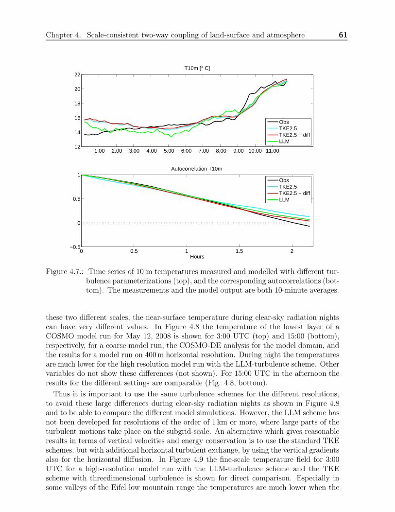
Chapter 4. Scale-consistent two-way coupling of land-surface and atmosphere 61
1:00 2:00 3:00 4:00 5:00 6:00 7:00 8:00 9:00 10:00 11:0012
14
16
18
20
22T10m [° C]
ObsTKE2.5TKE2.5 + diffLLM
0 0.5 1 1.5 2−0.5
0
0.5
1
Hours
Autocorrelation T10m
ObsTKE2.5TKE2.5 + diffLLM
Figure 4.7.: Time series of 10 m temperatures measured and modelled with different tur-bulence parameterizations (top), and the corresponding autocorrelations (bot-tom). The measurements and the model output are both 10-minute averages.
these two different scales, the near-surface temperature during clear-sky radiation nightscan have very different values. In Figure 4.8 the temperature of the lowest layer of aCOSMO model run for May 12, 2008 is shown for 3:00 UTC (top) and 15:00 (bottom),respectively, for a coarse model run, the COSMO-DE analysis for the model domain, andthe results for a model run on 400m horizontal resolution. During night the temperaturesare much lower for the high resolution model run with the LLM-turbulence scheme. Othervariables do not show these differences (not shown). For 15:00 UTC in the afternoon theresults for the different settings are comparable (Fig. 4.8, bottom).
Thus it is important to use the same turbulence schemes for the different resolutions,to avoid these large differences during clear-sky radiation nights as shown in Figure 4.8and to be able to compare the different model simulations. However, the LLM scheme hasnot been developed for resolutions of the order of 1 km or more, where large parts of theturbulent motions take place on the subgrid-scale. An alternative which gives reasonableresults in terms of vertical velocities and energy conservation is to use the standard TKEschemes, but with additional horizontal turbulent exchange, by using the vertical gradientsalso for the horizontal diffusion. In Figure 4.9 the fine-scale temperature field for 3:00UTC for a high-resolution model run with the LLM-turbulence scheme and the TKEscheme with threedimensional turbulence is shown for direct comparison. Especially insome valleys of the Eifel low mountain range the temperatures are much lower when the
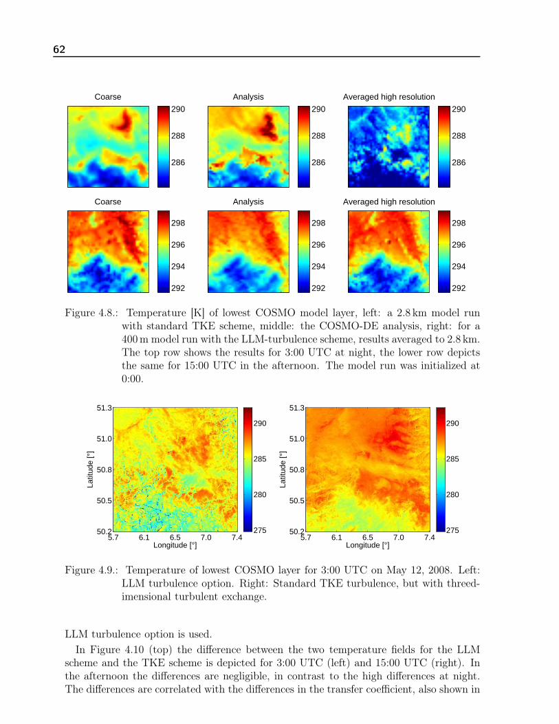
62
Coarse
286
288
290
Analysis
286
288
290
Averaged high resolution
286
288
290
Coarse
292
294
296
298
Analysis
292
294
296
298
Averaged high resolution
292
294
296
298
Figure 4.8.: Temperature [K] of lowest COSMO model layer, left: a 2.8 km model runwith standard TKE scheme, middle: the COSMO-DE analysis, right: for a400m model run with the LLM-turbulence scheme, results averaged to 2.8 km.The top row shows the results for 3:00 UTC at night, the lower row depictsthe same for 15:00 UTC in the afternoon. The model run was initialized at0:00.
Longitude [°]
Latit
ude
[°]
5.7 6.1 6.5 7.0 7.4
51.3
51.0
50.8
50.5
50.2 275
280
285
290
Longitude [°]
Latit
ude
[°]
5.7 6.1 6.5 7.0 7.4
51.3
51.0
50.8
50.5
50.2 275
280
285
290
Figure 4.9.: Temperature of lowest COSMO layer for 3:00 UTC on May 12, 2008. Left:LLM turbulence option. Right: Standard TKE turbulence, but with threed-imensional turbulent exchange.
LLM turbulence option is used.
In Figure 4.10 (top) the difference between the two temperature fields for the LLMscheme and the TKE scheme is depicted for 3:00 UTC (left) and 15:00 UTC (right). Inthe afternoon the differences are negligible, in contrast to the high differences at night.The differences are correlated with the differences in the transfer coefficient, also shown in

Chapter 4. Scale-consistent two-way coupling of land-surface and atmosphere 63
Longitude [°]
Latit
ude
[°]
5.7 6.1 6.5 7.0 7.4
51.3
51.0
50.8
50.5
50.2 −5
0
5
Longitude [°]
Latit
ude
[°]
5.7 6.1 6.5 7.0 7.4
51.3
51.0
50.8
50.5
50.2 −5
0
5
Longitude [°]
Latit
ude
[°]
5.7 6.1 6.5 7.0 7.4
51.3
51.0
50.8
50.5
50.2 −0.01
−0.005
0
0.005
0.01
Longitude [°]
Latit
ude
[°]
5.7 6.1 6.5 7.0 7.4
51.3
51.0
50.8
50.5
50.2 −0.01
−0.005
0
0.005
0.01
Figure 4.10.: Top: Differences in temperature for May 12, 2008, 3:00 (left) and 15:00(right) UTC, LLM scheme minus TKE scheme. Bottom: the same for thetransfer coefficient.
Figure 4.10 (bottom): in regions where the transfer coefficient is higher, the temperatureis lower probably due to the stronger mixing in a stable atmosphere. The question arises,which of these two scenarios is more realistic.
A more detailed investigation of these differences should be carried out for more casestudies, by making use of observations of stations located in complex terrain. Satellitemeasurements might provide additional information. The influence of the different tuningparameters in the TKE turbulence scheme should be analyzed by sensitivity analyses.For this work this issue could not be investigated in more detail. For the evaluation ofthe downscaling implemented in the COSMO model, all model runs have been carriedout with the TKE turbulence scheme (with the the 3D-turbulence option, used for thehigh-resolution model runs) because this schemes is applicable for both scales and givessimilar results. An additional argument for this scheme is, that the results resemble theanalyses much more closely, which indicates a good performance, considering the analysesas “pseudo”-measurements.

64
Figure 4.11.: Concept of the mosaic approach including atmospheric downscaling. Thefluxes are computed separately for each subgrid pixel, and then averaged.The downscaling acts as a small-scale interface to the high-resolution SVATmodel.
Radiation
Clouds can cross several 400m grid boxes in a few minutes, thus a higher temporal fre-quency of radiation calculations is necessary. For consistency reasons for the developmentof the downscaling system, radiation computations are carried out on each atmosphericcolumn in all COSMO simulations. No averaging as in the COSMO-DE default setup iscarried out. The interval between two radiation calculations has been set to 3 minutes,which again leads to a significant increase in computation time due to the complexity ofthe radiation calculations.
4.2.5. The mosaic approach
In the mosaic approach (Seth et al., 1994), surface heterogeneities are accounted for byrunning the soil module, in this case TERRA, on an explicit higher resolution than theatmospheric part (Figure 4.11). The turbulent fluxes of latent and sensible heat needed bythe atmospheric model on the coarser atmospheric scale are obtained by averaging. Thenovel disaggregation scheme of the coarse atmospheric forcing data down to the resolutionof the soil module as developed in this work is described in section 4.3.
4.2.6. Data
Training data set
Eight high-resolution coupled model runs for different weather situations (Table 4.1) havebeen carried out to build a high-resolution data base for the downscaling scheme. The firsttwo hours of each model run were discarded to remove spin-up effects. Days with calm,clear-sky weather, days with unstable convective situations and days with strong synopticforcing were chosen to cover the dominant weather situations. Cases with homogeneousstratiform cloud cover are included, as well as cases with fast moving clouds under stormyconditions.

Chapter 4. Scale-consistent two-way coupling of land-surface and atmosphere 65
Table 4.1.: Overview of simulated days including prevailing weather situation.
Date Weather situation
Training
27 August 2007 varying cloud cover, no precipitation14/15 October 2007 clear sky
3 March 2008 strong winds, variable clouds and precipitation1/2 May 2008 clouds and precipitation9/10 May 2008 clear sky
8 June 2008 convective clouds and precipitation21 July 2008 synoptically driven stratiform rainfall
28 August 2008 cloudy, some rainValidation
12 May 2008 calm, only sparse cloud cover15 May 2008 convective clouds, showers and thunderstorms16 July 2008 stratiform rain
20 October 2009 cirrus clouds, no rain21 October 2009 some clouds26 January 2010 fog in the morning, clear sky later
Validation data: Case studies
The downscaling scheme has been validated offline by applying it to COSMO outputand comparing the results to high-resolution reference output. For this purpose threedays with very different weather types (see also Table 4.1) have been chosen: May 12,2008 was characterized by very calm weather conditions. Central Europe was under theinfluence of a stable high pressure system for several days. Precipitation was absent andonly few clouds were observed. During May 15, 2008, Central Europe was under theinfluence of several low pressure systems situated over the Atlantic ocean and northernEurope. The high pressure system was weakening and moved to south-eastern Europe.Under these rather unstable conditions the model domain was almost completely coveredby convective clouds during the whole day, including showers and thunderstorms. OnJuly 16, 2008 a low pressure system over the northern Atlantic influenced the weatherconditions in Central Europe, with a cold front crossing Northern Germany during theday. The strong synoptical forcing led to stratiform rainfall and homogeneous cloud coverover the model domain.
For the “online” validation, i.e. the evaluation of the fully coupled mosaic-downscalingsimulations, three additional days with calm weather have been simulated (the last threedays in Table 4.1), because for calm days the effect of subgrid-scale heterogeneity is morevisible and more important than for advective, synoptically forced days.

66
Figure 4.12.: Temperature at the lowest atmospheric model level on 9 May, 2008 at 12:00UTC in Kelvin at 2.8 km resolution (left), 400m resolution (middle) and theanomalies, i.e. the differences between both (right).
Table 4.2.: Downscaled variables
Variable Abbreviation
Temperature at lowest model layer TSpecific humidity at lowest model layer qv
Wind speed at lowest model layer |vh|Shortwave net radiation flux at surface SnetLongwave net radiation flux at surface Lnet
Precipitation (rain, snow, graupel) PRECSurface pressure PS
4.3. The downscaling approach
Stepwise downscaling approach
A downscaling scheme should recover as good as possible the original fine-scale field (400mgrid spacing, for an example temperature field see Fig. 4.12, middle) from the coarse field(2.8 km grid spacing, Fig. 4.12, left). This is equivalent to predicting the anomalies (Fig.4.12, right) based on the coarse atmosphere resolution and the high-resolution land surfaceinformation. For training and development of the downscaling scheme these anomalieswere obtained by averaging the high-resolution model output to the 2.8 km scale, andsubtracting these coarse values from the original 400m model output. Downscaling isnecessary for those atmospheric variables which are needed as input for a SVAT model (inour case TERRA) or hydrological models, which are usually driven by the same variablesas a SVAT model (see Table 4.2).
The disaggregation system comprises three steps, which can be applied individually orsubsequently, depending on the variable and the application under consideration. The

Chapter 4. Scale-consistent two-way coupling of land-surface and atmosphere 67
first step interpolates the coarse resolution to the fine resolution by bi-quadratic splinesin x- and y-direction, while conserving mean and gradients of the coarse field. The sec-ond step exploits empirical relations between atmospheric variables and surface variablesusing high-resolution surface information (“deterministic” downscaling rules). The thirdstep adds the still missing high-resolution variability by adding noise. Thus downscalingsteps 1 and 2 reconstruct the high-resolution fields as accurately as possible, and step 3replenishes the mostly too low small-scale variability up to the variability of the high-resolution simulations. Since step 3 will usually increase the error, a decision between lowerrors (apply only downscaling step 1 and 2) or a realistic small-scale variance (apply alsostep 3) has to be made. These steps are explained in detail in the following (as publishedin Schomburg et al., 2010)
4.3.1. Step 1: Spline interpolation
The average conserving bi-quadratic spline equation used in the first step
f(x, y) = a1 + a2x+ a3y + a4x2 + a5y
2 (4.2)
requires five unknown coefficients for every coarse pixel. Thus five constraints have tobe formulated. Four constraints are provided by the derivatives of equation 4.2 at theedges between the coarse pixels, which are set to be equal to the derivative of the coarsefield perpendicular to the edges. The conservation of the mean value serves as the fifthconstraint.
4.3.2. Step 2: Deterministic downscaling rules
The second step tries to recover the difference between the spline interpolated field andthe original high-resolution field with deterministic rules. For these rules high-resolutionsurface information is used as predictor based on linear regression.
Some variables can be downscaled by exploiting known physical relationships. By thismeans the surface pressure anomaly can be downscaled by using the relief height anomaly∆z in the hydrostatic equation
∆p = −ρg∆z. (4.3)
For simplicity a constant air density has been assumed, in a least-squares fit ρ=1.19 kgm-3
gave the best results.The shortwave net radiation at the surface can be split up into
Snet = Sdir ↓ +Sdif ↓ −Sdif ↑ (4.4)
with Sdir ↓ the incoming direct radiation from the sun, Sdif ↓ the diffuse downwellingradiation and Sdif ↑ the reflected diffuse upwelling radiation. The downscaled diffuseupwelling radiation can be obtained from the high-resolution surface albedo for directand diffuse light, αdir and αdif , via
Sdif ↑= αdirSdir ↓ +αdifSdif ↓ . (4.5)
68
The downwelling direct and diffuse radiation are not correlated with surface variables.Both have little subgrid heterogeneity in cloud free cases (the average subgrid-scale stan-dard deviation is 2Wm-2), while in cloudy situations their subgrid-scale variability relatesto cloud cover variability on the subgrid-scale (the average subgrid-scale standard devi-ation is 39Wm-2). Thus, in rather homogeneous cloudfree conditions the shortwave netradiation can be disaggregated with near perfect correlation because all subgrid variabilityis associated with surface (albedo) variability. Under cloudy conditions the variability hasto be induced by stochastic methods (in step 3).
For the remaining variables (temperature, humidity, wind speed, precipitation and long-wave radiation) the situation is less intuitive. Thus the high-resolution data base was sta-tistically evaluated for possible correlations between atmospheric and surface variables.However, usually such correlations are not generally valid, but depend on the prevailingweather conditions. Figure 4.13 depicts the spatially averaged correlation between thetemperature anomalies of the lowest atmospheric model layer and the topographic heightanomalies (both with respect to the 2.8 km scale) for a clear sky day. Correlations are closeto minus one during the day, as one would expect for a well mixed boundary layer. Thestratification leads to a simple decrease of temperature with topographic height, whichcan be exploited for the disaggregation of the high-resolution atmospheric near-surfacetemperature anomalies. During clear-sky nights, however, when outgoing longwave ra-diation leads to strong cooling of the ground, no or only a slightly positive correlationbetween temperature and elevation exists. Nighttime inversions and complex valley circu-lations destroy any usable statistical predictions. Thus prior to the use of the orographichigh-resolution surface information as predictor for near surface temperatures, the tem-perature gradient of the lower atmosphere is computed and a decision made, based on itscloseness to adiabatic stratification (see Fig. 4.13, bottom). For illustration the corre-lations without and with application of the temperature gradient as indicator are shownas scatterplots in Figure 4.14. The statistical correlation between temperature and reliefanomalies is very low for the complete data base (Fig. 4.14a); using the coarse-resolutiontemperature gradient as pre-selection criterion, however, a strong negative correlationexists (Fig. 4.14b).
To find the most suitable predictors, indicators and thresholds, an automatic rule de-tection system has been developed. In this system the correlations between all possiblepredictors and the desired downscaled variables are calculated, based on indicators, whichmight allow or disallow the rule. The corresponding indicator thresholds are varied be-tween the minimum and maximum value found in the data base for each possible indicatorvariable in 30 steps. For 5 predictands, 16 possible predictors, 24 possible indicators, (seeTable 4.3 for a list of all provided predictors and indicators), 30 indicator-range intervals,and the whole procedure performed 2 times (testing for situations where the indicatoris larger or smaller than the threshold, respectively), a total of 5*16*24*30*2=115,200correlations were computed. The automatic rule search system is sketched in Figure 4.15.Only those rules are selected, which lead to correlation coefficients above 0.7, i.e. an ex-plained variance of at least 50%. The final selection of a rule requires in addition, that therule is applicable to at least 10% of the data. Table 4.4 contains all rules detected by thisautomatic search system. If several indicators were found describing similar situations,only the indicator applicable to the larger part of the data set is chosen. If more than

Chapter 4. Scale-consistent two-way coupling of land-surface and atmosphere 69
0 6 12 18 24 6 12 18 24−1
−0.5
0
0.5
Cor
rela
tion
[ ]
Time [UTC]
0 6 12 18 24 6 12 18 24−0.02
0
0.02
0.04
T−
grad
ient
[K/m
]
Time [UTC]
Figure 4.13.: Top: Correlations between temperature anomalies in 10m and orographicanomalies with respect to the coarse pixel scale of 2.8 km for 9 May 2008,a clear sky radiation day. Bottom: mean coarse scale vertical temperaturegradient of the lowest four model layers.
(a) (b)
Figure 4.14.: Scatterplot of temperature anomalies versus orographic height anomalieswith respect to the coarse pixel scale of 2.8 km. a) all cases. b) only wherethe coarse temperature gradient of the lowest 105m is below a threshold of0.0057Km-1, with a linear fit.

70
Figure 4.15.: The automatic rule search system: For all possible predictands y and pre-dictors x the correlations for all cases in the data set larger (or smaller) thana certain threshold t of all possible indicators I are computed. If the corre-lation is larger than 0.7 this relationship is stored as a downscaling rule. Ifnot the threshold is further increased (or decreased).
one predictor is found for the desired variable, its usefulness was evaluated by a stepwiseregression. As a final step for each of the downscaled variables the coefficients needed fora linear regression between downscaling variable and predictors have been computed.
For the near surface temperature several rules have been found, indicating that thisvariable is closely related to relief height or temperature gradient multiplied with reliefheight, with the coarse temperature gradient as indicator. In the end only the rule usingorographic information in situations indicated by the temperature gradient of the lowest105 m was taken as a rule, because it covered the largest part of the data base (64%);using other predictors did not give substantial additional skill.
For specific humidity and wind speed no exploitable correlations with surface quantitieshave been found. Setting the desired correlation in the automatic search system to a lowervalue, i.e. 0.5 (instead of 0.7 as before), correlations between near surface humidity qv andsurface humidity qvsfc of 0.51 for 12% of the cases were found, detectable by the humiditygradient of the lowest two atmospheric layers. This rule has been discarded for the currentsetup due to the low correlation. Correlations between qv and qvsfc can change strongly inshort time periods, which might explain the difficulty to find useful rules for the specifichumidity. In Figure 4.16 the subgrid correlations between qv and qvsfc are shown forthree consecutive hours of May 12, 2008. While at 6:00 UTC no systematic correlationsare detectable, at 7.00 UTC the correlations are strongly positive on the north-westernpart of the model domain and anti-correlated in most regions. Only one hour later thecorrelations between qv and qvsfc are close to one for almost the whole domain.
With the same criterion also a relationship between wind speed and sensible heat fluxwas found; this relationship was discarded, however, because of the dependency of thesensible heat flux on wind speed. Also averaging the near surface and the surface quantitiesover an hour did not lead to usable correlations for wind speed or specific humidity.The fields of qv and |vh| at the lowest atmospheric layer contain many transient small-

Chapter 4. Scale-consistent two-way coupling of land-surface and atmosphere 71
Table 4.3.: Possible predictors (available on high resolution) and indicators (coarse resolu-tion) for the deterministic downscaling. The predictors gradients×orographyare computed by using the coarse temperature gradient information (fine scaleinformation is usually not available) and the fine scale surface information onthe relief height.
Possible predictors Possible indicators
TG Ground temperature [K] Tgr25Temperature gradient of lowest 2layers (25 meters) [Km−1]
H Orography [m] Tgr60Temperature gradient of lowest 3layers (60 meters) [Km−1]
LAI Leaf area index [1] Tgr105Temperature gradient of lowest 4layers (105 meters) [Km−1]
z0 Roughness length [m] qvgr25Specific humidity gradient of lowest2 layers (25 meters) [m−1]
ln(z/z0)Logarithmic roughness ratio be-tween height of lowest model layerand roughness length [1]
qvgr60Specific humidity gradient of lowest3 layers (60 meters) [m−1]
qvsfc Specific humidity at surface [kg/kg] qvgr105
Specific humidity gradient of lowest4 layers (105 meters) [m−1]
Tgr25× HTemperature gradient of lowest 2layers (25 meters) × orography [K]
µ Cosine of solar zenith angle [1]
Tgr60× HTemperature gradient of lowest 3layers (60 meters) × orography [K]
LWP Liquid water path [kgm−2]
Tgr105× HTemperature gradient of lowest 4layers (105 meters) × orography [K]
LWPvarLWP variance of 3x3 coarse pixels[kg2m−4]
qvgr25× HSpecific humidity gradient of lowest2 layers (25 meters) × orography [1]
OROvarOrography variance of 3x3 coarsepixels [m2]
qvgr60× HSpecific humidity gradient of lowest3 layers (60 meters) × orography [1]
|vh| Wind speed [m/s]
qvgr105× HSpecific humidity gradient of lowest4 layers (105 meters) × orography[1]
DD Wind direction [◦]
(Fh)sfc Sensible heat flux [Wm−2] UNear-surface u-wind component[m/s]
(Fqv)sfc Latent heat flux [Wm−2] VNear-surface v-wind component[m/s]
FRland Fraction of land [1] CLC Cloud cover [%]
WsoSoil moisture of top soil layer [mH2O]
CLC2
var
Cloud cover variance of 3x3 coarseneighboring pixels [%]
qv Near-surface specific humidity [1]RH Near-surface relative humidity [1]
(qvsfc)var
Variance of 3x3 neighboring pixelsof surface specific humidity [1]
SnetShortwave net radiation at surface[Wm−2]
LnetLongwave net radiation at surface[Wm−2]
PS Surface pressure [Pa]PREC Precipitation [kgm−2s−1]FRland Fraction of land [1]

72
Table 4.4.: Deterministic downscaling rules found by the automatic rule search algorithm.Shown are relationships between the downscaling variables, i.e. the predic-tands, and possible predictors for indicators above or below a certain thresholdof the indicator value. At least a correlation above 0.7 between predictor andpredictand was necessary, and at least 10% of all cases of the data set needsto be covered by this rule. For abbreviations of the variables see Tables 4.2and 4.3 and the list of symbols in the appendix B.
Predictand Predictor Indicator with threshold Correlation Data coverage [%]
T Tgr105 ∗H Tgr105 < 0.0022 0.74 59
Tgr60 < 0.0037 0.75 58
Tgr25 > 0.0065 0.75 56
|vh| > 5.1 0.71 12
LWP > 0.095 0.71 10
U > 3.2 0.71 17
Snet > 204 0.81 29
Tgr60 ∗H Tgr105 < 0.0022 0.71 59
Tgr60 < 0.0037 0.74 58
Tgr25 < 0.0065 0.76 56
U > 3.7 0.78 13
Snet > 204 0.81 29
Tgr25 ∗H Tgr105 < −0.0048 0.82 47
Tgr60 < −0.00155 0.78 52
Tgr25 < 0.0065 0.72 56
Snet > 204 0.78 29
H Tgr105 < 0.0058 -0.74 64
Tgr60 < 0.0090 -0.73 64
Tgr25 > 0.0161 -0.72 63
µ > 0.82 -0.7 17
|vh| > 4.0 -0.76 23
LWP > 0.095 -0.78 10
U > 3.2 -0.78 17
Snet > 179 -0.72 31
Lnet > −15.224 -0.7 17
Lnet Tg clc < 43 -0.72 38
Lnet < −82.5 -0.74 36
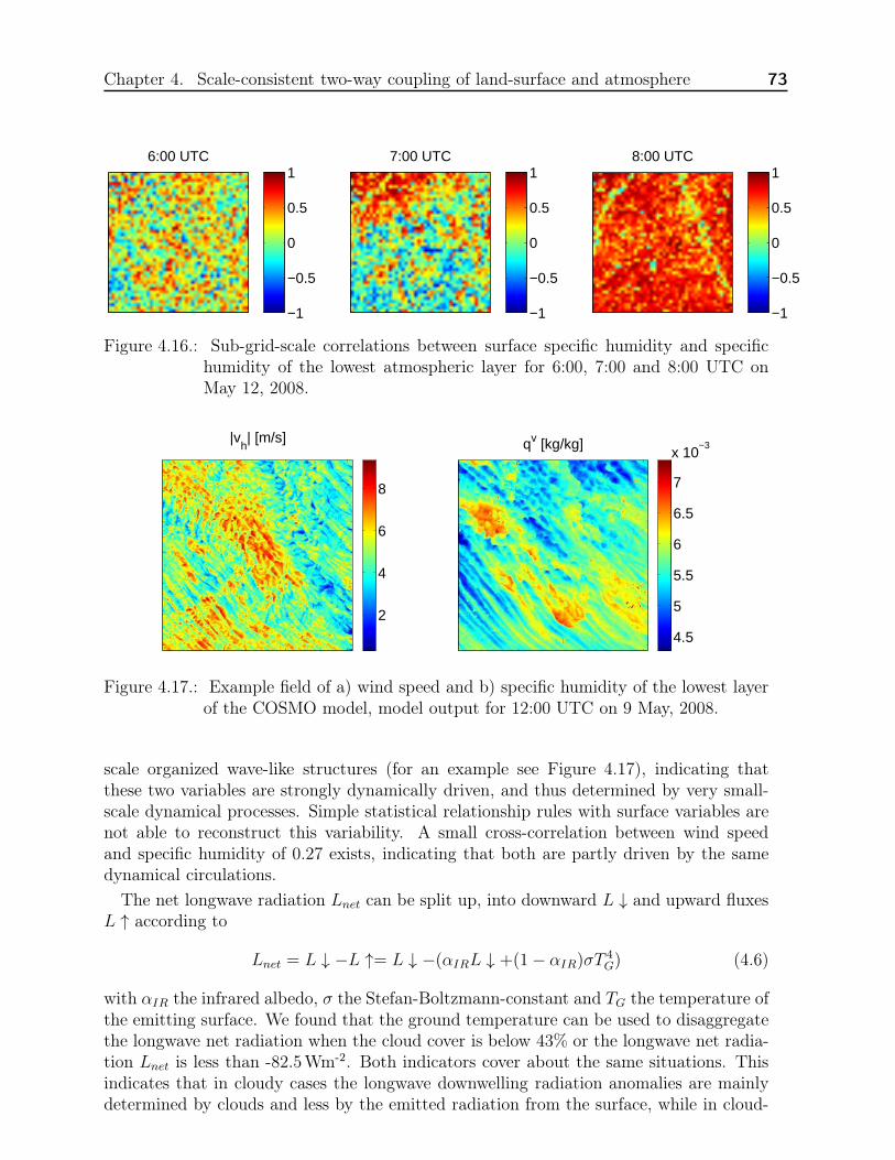
Chapter 4. Scale-consistent two-way coupling of land-surface and atmosphere 73
6:00 UTC
−1
−0.5
0
0.5
17:00 UTC
−1
−0.5
0
0.5
18:00 UTC
−1
−0.5
0
0.5
1
Figure 4.16.: Sub-grid-scale correlations between surface specific humidity and specifichumidity of the lowest atmospheric layer for 6:00, 7:00 and 8:00 UTC onMay 12, 2008.
|vh| [m/s]
2
4
6
8
qv [kg/kg]
4.5
5
5.5
6
6.5
7
x 10−3
Figure 4.17.: Example field of a) wind speed and b) specific humidity of the lowest layerof the COSMO model, model output for 12:00 UTC on 9 May, 2008.
scale organized wave-like structures (for an example see Figure 4.17), indicating thatthese two variables are strongly dynamically driven, and thus determined by very small-scale dynamical processes. Simple statistical relationship rules with surface variables arenot able to reconstruct this variability. A small cross-correlation between wind speedand specific humidity of 0.27 exists, indicating that both are partly driven by the samedynamical circulations.
The net longwave radiation Lnet can be split up, into downward L ↓ and upward fluxesL ↑ according to
Lnet = L ↓ −L ↑= L ↓ −(αIRL ↓ +(1− αIR)σT4G) (4.6)
with αIR the infrared albedo, σ the Stefan-Boltzmann-constant and TG the temperature ofthe emitting surface. We found that the ground temperature can be used to disaggregatethe longwave net radiation when the cloud cover is below 43% or the longwave net radia-tion Lnet is less than -82.5Wm-2. Both indicators cover about the same situations. Thisindicates that in cloudy cases the longwave downwelling radiation anomalies are mainlydetermined by clouds and less by the emitted radiation from the surface, while in cloud-

74
Table 4.5.: Deterministic rules with the respective regression coefficients, correlationsachieved and amount of data covered.
Down-scalingvariable
Predic-tor
ConstraintRegression coeffi-cient
CorrelationDatacove-rage
T H Tgr105<0.0058 -0.0084Km-1 0.74 64%
Lnet TG Lnet<-82.5 -3.878 Wm-2K-1 0.74 36%
PS H - -11.694Pam-1 1.0 100%
free situations the longwave emission from the surface is the only source of heterogeneity.
As expected for these small scales no rules have been found for precipitation. In Table4.5 the regression coefficients, correlation achieved and data coverage for the rules foundby the automatic rule detection system are listed. The regression coefficients are basedon the same data base as was used for the rule detection system (see Table 4.1).
4.3.3. Step 3: Noise generation
Except for surface pressure the downscaling steps 1 and 2 alone do not reproduce all small-scale variability contained in the simulated high-resolution fields. The full variance is,however, important for modeling the nonlinear processes at the surface. Lower variabilitiescan lead to biases in the computed fluxes when averaged over larger spatial and temporalscales. To avoid these biases, the yet unresolved variance is added as noise, at the expenseof a higher error at the smallest scale. This third step is applied after carrying out thefirst two downscaling steps, or, for the variables for which no deterministic relationshipcan be found, directly after step 1.
Estimating the small-scale variance
In Figure 4.18 the subgrid-scale variances for temperature for different hours of the day areshown, for a clear-sky radiation day (top) and a day with stratiform homogeneous cloudcover (bottom). The subgrid variance under clear-sky conditions is larger during nightthan during mid-day and under stratiform synoptically driven conditions. This showsthat before adding the missing small-scale variability, this missing variability first needsto be assessed, as it may vary considerably for different synoptic conditions and also fordifferent variables.
A stepwise multiple linear regression system has been developed, which estimates thesmall-scale standard deviation based on the coarse-scale standard deviation of the sur-rounding 3x3 coarse pixels and other atmospheric variables, which serve as a measure forthe atmospheric conditions. For each variable variance different predictors have been cho-sen by the stepwise regression (Table 4.6). For completeness the exact regression equationsare given:

Chapter 4. Scale-consistent two-way coupling of land-surface and atmosphere 75
2:00 UTC
0
1
2
38:00 UTC
0
1
2
314:00 UTC
0
1
2
320:00 UTC
0
1
2
3
2:00 UTC
0
1
2
38:00 UTC
0
1
2
314:00 UTC
0
1
2
320:00 UTC
0
1
2
3
Figure 4.18.: Subgrid-scale variance for temperature (in Kelvin) per coarse pixel for afair-weather day (9 May, 2008, top) and a day with stratiform cloud cover(21 July, 2008, bottom) for different hours of the day.
Table 4.6.: Predictors for estimating the standard deviation (stddev) at the small scale.
Downscaling variable Predictors
T Tgr25, 3x3 coarse stddev, PSqv 3x3 coarse stddev|vh| 3x3 coarse stddev, PSSnet 3x3 coarse stddevLnet 3x3 coarse stddev, subgrid stddev of qvsfc
σT = 4.3255 ∗ Tgr25 + 0.5026 ∗ σ3x3c − 1.5497 · 10−5 ∗ PS + 1.6125
σ|vh| = 0.7762 ∗ σ3x3c − 4.2692 · 10−5 ∗ PS + 4.5029
σqv = 0.7076 ∗ σ3x3c + 1.2202 · 10−5
σSnet= 0.8882 ∗ σ3x3
c + 4.2606
σLnet= 0.7 ∗ σ3x3
c + σqvs.
σ3x3c is the standard deviation of the respective variable of the 3x3 surrounding grid boxes,
and σqvs is the subgrid-scale standard-deviation of surface specific humidity.For variables for which downscaling step 2 has been applied, the variance generated by
step 2 is subtracted from the estimated value from the regression to add only the stillmissing variance.
Algorithm for noise generation
The noise is modeled based on an autoregressive process, to account for its temporallycorrelated nature.
xnew = φxold + ǫ (4.7)

76
where ǫ is a Gaussian noise term. The correlated noise has a zero mean value, becauseonly the anomalies are reconstructed. To compute the intermediary autoregression noiseterm xnew with a standard deviation of unity, the standard deviation of ǫ is computedaccording to:
σǫ =√
1− φ2; (4.8)
The autoregression coefficient φ is obtained by carrying out one or several model runswith high-resolution temporal output, and computing the autocorrelation for the desiredvariable and time lag. The coarse model at 2.8 km grid spacing (for the atmosphere) hasa time step of 25 seconds, and the respective lag-1 autocorrelations φ were found to liebetween 0.92 for the shortwave radiation and 0.97 for the specific humidity. The finalnoise field, which is added to the coarse field, is then obtained by
xnoise = σmissxnew (4.9)
where σmiss is the missing standard deviation estimated above. Spatial correlations areignored in this step, in contrast to the first two steps. Addition of noise including thecorrect spatial correlations is planned for a future extension of the scheme.
For all downscaling steps the coarse mean of the grid cell is conserved by subtractingthe difference between the coarse value and the mean of the downscaled values, ensuringthe conservation of energy and mass. In very rare cases negative values of wind speed,shortwave radiation or precipitation result from the statistical downscaling which shouldnot be used to force a soil model or a hydrological model. Thus, negative values are setto zero (or to the mean value for wind speed). The mean value of the coarse pixel is thenconserved by multiplying the subgrid-pixel values by the fraction of the coarse meansbefore and after setting these pixels to zero.
Precipitation
The downscaling of precipitation is treated as a special case, because additive noise couldlead to negative precipitation values. Moreover Gaussian noise does not model the dis-tribution of the anomalies well. The precipitation noise-generation algorithm consistsof three steps. First, autoregressive Gaussian noise g is generated. This noise is thentransformed into the following distribution, setting values below a threshold to zero andtransforming the other values by a power law:
t = e(a∗(g+b)) (4.10)
The noise values t are subsequently multiplied by the coarse mean precipitation. Theconstants, i.e. the threshold, the fitting parameter a and b and the autoregressive constant,are optimized to fit with the distribution and the autocorrelation function of two modelruns with high temporal resolution output that produced precipitation.
The different precipitation classes rain, snow and graupel are summed up and down-scaled together as one precipitation class. After the downscaling they are again split upaccording to their original fractions.

Chapter 4. Scale-consistent two-way coupling of land-surface and atmosphere 77
Cross correlations
The automatic rule search algorithm described in section 4.3.2 has also been appliedto search for possible cross correlations between the atmospheric downscaled variables.An overall cross correlation between wind speed and specific humidity of −0.27 (takingthe whole data base into account) has been found. Shortwave and longwave radiationnet fluxes are correlated by -0.52 in cloudy conditions, i.e. if CLC > 0. These cross-correlations have been emulated in the noise-generating process
ǫ′ψ =√
(1− |σcross|)ǫψ +√σcrossǫcross (4.11)
where ǫψ is the noise term for a variable ψ in equation (4.7) and σcross is the respectivecross correlation between two variables.
4.4. Results
In this section first the results of the different downscaling steps, applied to the variousvariables are shown (published in Schomburg et al., 2010). In section 4.4.2 offline applica-tions of the downscaling to compute the fluxes are shown, and in section 4.4.3 the resultsof the downscaling implemented in the COSMO model itself and used in combinationwith the mosaic approach are given.
4.4.1. Disaggregation results for variables
The scheme has been tested for three case studies as described in section 4.2.6, i.e. a calmsunny day, a convective showery day and a stratiform rainy day.
The first downscaling step reduces already considerably the root mean square errors ofthe downscaled field for all variables, when compared to the coarse resolution field with thehigh-resolution model output as reference. A standard bi-linear interpolation algorithmusing the four surrounding values, which has been tested for comparison only, does notlead to such a strong error reduction; here the errors are reduced only slightly, i.e. thebi-quadratic spline interpolation leads to better results, see Table 4.7 (top). Moreover, abi-linear interpolation does not allow to conserve the coarse average to the same degreeas the bi-quadratic interpolation (Tab. 4.7, bottom).
In Figure 4.19 the results of the individual downscaling steps and the final results for atemperature field of the lowest atmospheric layer are shown. The coarse field (Fig. 4.19a)is smoothed by the average conserving splines (step 1, Fig. 4.19e). After calculating thetemperature anomalies, using relief height as predictor (step 2, Fig. 4.19b) and addingthese to the result from the first step (Fig. 4.19f), the still missing variance is estimatedand added as spatially uncorrelated noise in step 3 (Fig. 4.19c). These three stepstogether add up to the final field (Fig. 4.19g), which resembles closely the original finescale field (Fig. 4.19h). In this example the deterministic downscaling yields very goodresults, hence the true anomalies (Fig. 4.19d) are well reproduced in downscaling step2 (Fig. 4.19b). In contrast, in Figure 4.20 a case is shown where the deterministicdownscaling has less skill. During a clear, cloudfree night, the air temperature does notdecrease adiabatically with height, therefore the deterministic downscaling rule can only

78
Table 4.7.: Root mean square errors of the coarse field, a high-resolution field obtained bythe bi-quadratic spline interpolation (downscaling step 1) and for comparison ahigh-resolution field generated by a standard bi-linear interpolation, spatiallyand temporally averaged for May 15, 2008. Top: RMSE for the small scale,bottom: RMSE for coarse scale.
Field T [K] |vh| [m/s] qv [kg/kg] PS [Pa]Snet
[W/m2]Lnet
[W/m2]PREC[kg/m2]
400m scale
Coarse 0.26 0.42 1.62e-04 282 20.2 4.36 2.10e-04Bi-linear 0.24 0.40 1.47e-04 260 19.5 4.15 1.98e-04Bi-quadratic 0.23 0.38 1.33e-04 236 18.3 3.91 1.75e-04
2.8 km scale
Coarse 0 0 0 0 0 0 0Bi-linear 0.10 0.13 6.2e-05 109 6.75 1.40 8.8e-05Bi-quadratic 6.2e-04 9.4e-04 4.2e-07 0.75 0.05 0.01 6.2e-07
be applied to a very small part of the model domain (Figure 4.20a). Thus the main partof the subgrid-scale variability is generated by the noise generation step (Fig. 4.20b).Since the spatial subgrid-scale correlations are not modelled, the spatial characteristics ofthe true anomalies (Fig. 4.20c) are not well reconstructed. In the original field cold airgathers in some of the valleys, which cannot be recovered by a simple statistical method.
Figure 4.21 shows an example for the downscaling of longwave net radiation at thesurface. We start again from the coarse field (Fig. 4.21a), apply the spline interpolation(Fig. 4.21e), and add the deterministic anomaly proportional to the surface temperatureanomalies, which leads to the intermediate field Fig. 4.21f. The addition of noise (step3) finally leads to Figure 4.21g. In the original field (Fig. 4.21d and h) a small region inthe northeastern part shows particular large small-scale variability. This large scatter isnot reconstructed in step 2 (Fig. 4.21b), because this variability is not caused by surfaceheterogeneity but by some sparse clouds. The missing variance is satisfactorily replenishedby step 3 (Fig. 4.21c).
The time series of the root mean square errors (RMSE) produced by the individualdownscaling steps is shown in Figure 4.22 for a case study of May 12, 2008. The firststep (spline interpolation) leads for all variables to a small error reduction compared tothe coarse fields (here the error of the coarse field at the small scale is computed byassuming homogeneous forcing for all sub-pixels). Where applicable, i.e. for temperature,pressure and the radiation fluxes, the deterministic downscaling leads to a considerableerror reduction. The error reduction for temperature (Fig. 4.22a) during the clear skynight is less distinctive than during the day. These problems do not exist during overcastnights (not shown). Adding random noise in the third step naturally increases the RMSEerror for most variables (temperature at night, humidity, wind speed and the radiationfluxes in the evening, in this case); sometimes the RMSE even exceeds the RMSE of thehomogeneous field.
As mentioned above, the correct subgrid-scale variability can be decisive to avoid biasesfor applications involving nonlinear processes. The first downscaling step introduces somevariance (see Fig. 4.23). The second step leads to a another large increase of the high-

Chapter 4. Scale-consistent two-way coupling of land-surface and atmosphere 79
Coarse
291.5
292
292.5
293
293.5
294
294.5
(a)
Deterministic anomaly
−1
−0.5
0
0.5
1
(b)
Noise
−1
−0.5
0
0.5
1
(c)
True anomaly
−1
−0.5
0
0.5
1
(d)Step 1
291.5
292
292.5
293
293.5
294
294.5
(e)
Step 1 + 2
291.5
292
292.5
293
293.5
294
294.5
(f)
Step 1+2+3
291.5
292
292.5
293
293.5
294
294.5
(g)
Original field
291.5
292
292.5
293
293.5
294
294.5
(h)
Figure 4.19.: Downscaling scheme applied to a temperature field (in Kelvin) of the lowestatmospheric model layer, 10:00 UTC, May 12th, 2008. Top: a) coarse field;b) deterministic anomaly; c) generated noise; d) true anomaly. Bottom:Temperature field after application of e) step 1 (spline interpolated); f) step1 + 2; g) step 1 + 2 + 3 (final field, i.e. sum of all three downscaling steps);h) original fine scale field (reference).
resolution standard deviation. Even more subgrid variability is generated by step 3, inwhich the still missing variance is estimated and added. The subgrid heterogeneity is wellparameterized, but temporary deviations from the reference do occur. For pressure thethird step is not applied, because the variability generated in the second downscaling stepis already sufficient (see Fig. 4.23d).
For comparison the root mean square errors and subgrid-scale standard deviations forMay 15, 2008, a convective showery day, are depicted in Figure 4.24. Results are shownonly for those variables which exhibit a different behaviour compared to the calm, sunnyday in the previous example. Here for the radiation fluxes almost no improvements canbe achieved by the second downscaling step, because the subgrid-scale variability is dom-inated by the heterogeneous cloud cover. The subgrid-scale standard deviation of theprecipitation is reproduced well for this day (Fig. 4.24f).
The errors and subgrid-scale variabilities are averaged spatially and temporally for thethree case studies and listed in Table 4.8 and 4.9. According to these results the errorsare reduced slightly by the first downscaling step and strongly by the second downscalingstep. The overall improvement gained for the radiation fluxes is less than for the single fairweather day shown in Fig. 4.22, because for the two other cloudy days the deterministicdownscaling step has much less skill. Only under clear sky conditions the RMSE is reducedconsiderably by the second downscaling step, otherwise the subgrid-scale variability is notdue to surface heterogeneity but to variable cloud cover. The subgrid-scale variability isenhanced slightly by downscaling step 1 and more by step 2 (where applicable) and step3 (Tab. 4.9). For all variables the subgrid standard deviation is on average slightly too

80
Deterministic anomaly
−1
−0.5
0
0.5
1
(a)
Noise
−1
−0.5
0
0.5
1
(b)
True anomaly
−1
−0.5
0
0.5
1
(c)
Figure 4.20.: Temperature anomalies (in Kelvin) constructed in downscaling step 2 (a)and downscaling step 3 (b) and reference anomalies for a clear-sky nighttimesituation, 1:00 UTC, May 12, 2008.
Coarse
−150
−140
−130
−120
−110
(a)
Deterministic anomaly
−15
−10
−5
0
5
10
15
(b)
Noise
−15
−10
−5
0
5
10
15
(c)
True anomaly
−15
−10
−5
0
5
10
15
(d)Step 1
−150
−140
−130
−120
−110
(e)
Step 1 + 2
−150
−140
−130
−120
−110
(f)
Step 1+2+3
−150
−140
−130
−120
−110
(g)
Original field
−150
−140
−130
−120
−110
(h)
Figure 4.21.: Same as Figure 4.19, but for the longwave surface net radiation in W/m2.
large after the last step, but only the deviations for wind speed, pressure and longwave netradiation are statistically significant. Obviously the mean statistics of these three daysdo not match the mean statistics of the training data set.
The temporal autocorrelations of the coarse fields are larger than those of the high-resolution reference values from the high-resolution fields (see Figure 4.25), this differenceprevails after application of downscaling steps 1 and 2. Step 3 leads to a strong decreaseof the autocorrelations with increasing time lags; for most variables the reference autocor-relations are now matched more closely. For precipitation the correlations are, however,too low after the third step.

Chapter 4. Scale-consistent two-way coupling of land-surface and atmosphere 81
1 4 7 10 13 17 20 230
0.2
0.4
0.6
0.8T
UTC
RM
SE
[K]
(a)1 4 7 10 13 17 20 23
0
0.5
1
1.5
|vh|
UTC
RM
SE
[m/s
]
(b)1 4 7 10 13 17 20 23
0
2
4
6
8x 10
−4 QV
UTC
RM
SE
[kg/
kg]
(c)
coarsestep 1step 1+2step 1+2+3
1 4 7 10 13 17 20 230
100
200
300PS
UTC
RM
SE
[Pa]
(d)1 4 7 10 13 17 20 23
0
10
20
30
Snet
UTC
RM
SE
[W/m
2 ]
(e)1 4 7 10 13 17 20 23
0
5
10
15
Lnet
UTC
RM
SE
[W/m
2 ]
(f)
Figure 4.22.: Timeseries of root mean square error (RMSE) of the downscaling variablesfor the three downscaling steps for May 12, 2008: a) temperature, b) windspeed, c) specific humidity, d) surface pressure, e) shortwave net radiation, f)longwave net radiation. For wind speed, specific humidity and precipitationthe deterministic step 2 is not applicable, see section 4.3.2.
Table 4.8.: Root mean square errors for the different variables for the downscaling stepsaveraged over the three case studies.
Disaggreg. T [K] |vh| [m/s] qv [kg/kg] PS [Pa] Snet[W/m2] Lnet[W/m2] PREC kg/m2
no disagg 0.31 0.56 1.54e-04 285 14.73 5.09 7.75e-05Step 1 0.27 0.52 1.34e-04 238 13.52 4.70 6.49e-05
Step 1+2 0.21 - - 6.2 12.18 4.15 -Step 1+2+3 0.31 0.82 1.94e-04 - 17.97 6.26 9.92e-05
Application to regional climate scale
The downscaling system was developed and tested for atmospheric variables based on400m grid spacing as the smaller scale and 2.8 km as the larger scale. First tests of thesystem for a disaggregation of the atmospheric variables from 14 km data down to 2.8 kmhave been conducted in order to see whether the system can also be used for regionalclimate simulations with the COSMO model on a 14 km grid, with surface information ona 2.8 km mosaic. Although the downscaling steps have been trained for smaller scales, theresults obtained by the downscaling are very encouraging in terms of root mean squareerror reduction (Fig. 4.26) and subgrid-scale variance reconstruction (Fig. 4.27). Thisindicates that the downscaling can be applied to other scales than the development scaleeven without making changes to the coefficients and rules.

82
1 4 7 10 13 17 20 230
0.2
0.4
0.6
0.8T
UTC
σ [K
]
(a)1 4 7 10 13 17 20 23
0
0.2
0.4
0.6
0.8
|vh|
UTC
σ [m
/s]
(b)1 4 7 10 13 17 20 23
0
2
4
6
8x 10
−4 QV
UTC
σ [k
g/kg
]
(c)
referencestep 1step 1+2step 1+2+3
1 4 7 10 13 17 20 23100
150
200
250PS
UTC
σ [P
a]
(d)1 4 7 10 13 17 20 23
0
10
20
30
Snet
UTC
σ [W
/m2 ]
(e)1 4 7 10 13 17 20 23
0
5
10
Lnet
UTC
σ [W
/m2 ]
(f)
Figure 4.23.: The same as Figure 4.22 for the subgrid-scale standard deviations (σ). Herethe black line denotes the reference subgrid standard deviations.
Table 4.9.: Sub-grid scale standard deviations for the different variables for the downscal-ing steps averaged over the three case studies.
Disaggreg. T [K] |vh| [m/s] qv [kg/kg] PS [Pa] Snet[W/m2] Lnet[W/m2] PREC kg/m2
Step 1 0.10 0.13 5.19e-05 105 3.52 1.23 1.16e-05Step 1+2 0.17 - - 225 6.03 1.94 -
Step 1+2+3 0.28 0.61 1.36e-04 - 13.37 4.72 2.50e-05Reference 0.27 0.52 1.35e-04 222 11.57 4.25 2.53e-05
4.4.2. Offline application of the downscaling system for
computing the turbulent fluxes
As a first step to understand the effects of the downscaling system on the turbulent fluxesof sensible and latent heat, the fluxes have been computed in an simple offline environmentby the flux equations:
(Fh)sfc = −ρKhL|vh|(T − Tsfc). (4.12)
(Fqv)sfc = −ρKhc|vh|(qv − qvsfc) (4.13)
The transfer coefficient Kh has also been computed offline by a simple transfer schemebased on a concept by Louis (1979), using Monin-Obukhov similarity theory. Output ofhigh-resolution (400m) model runs have been used as reference. The coarse values were(as before) obtained by averaging the small-scale values to the 2.8 km scale.
Five different configurations have been compared (see Table 4.10). Two kinds of down-scaling have been tested, a deterministic version applying only step one and two of thedisaggregation system (i.e. spline interpolation and deterministic rules), and a stochasticversion containing also step three, i.e. noise generation. These are compared with thestandard mosaic approach (i.e. with homogeneous atmospheric forcing for all mosaic-

Chapter 4. Scale-consistent two-way coupling of land-surface and atmosphere 83
1 4 7 10 13 17 20 230
0.5
1
1.5x 10
−3 PREC
UTC
RM
SE
[kg
m−
2 s−
1 ]
(a)1 4 7 10 13 17 20 23
0
50
100
Snet
UTC
RM
SE
[W/m
2 ]
(b)1 4 7 10 13 17 20 23
0
5
10
Lnet
UTC
RM
SE
[W/m
2 ]
(c)
1 4 7 10 13 17 20 230
1
2
3
4x 10
−4 PREC
UTC
σ [k
g m
−2 s
−1 ]
(d)
referencestep 1step 1+2step 1+2+3
1 4 7 10 13 17 20 230
20
40
60
Snet
UTC
σ [W
/m2 ]
(e)1 4 7 10 13 17 20 23
0
2
4
6
8
Lnet
UTC
σ [W
/m2 ]
(f)
Figure 4.24.: Top: Root mean square errors for shortwave and longwave radiation fluxesand precipitation for May 15, 2008. Bottom: The respective subgrid-scalevariances.
subpixels) and with the standard model grid without small scale information neither inthe atmosphere nor at the surface, i.e. without any subgrid heterogeneity representation.
For the comparisons, the fluxes have been computed on the fine scale and then averagedto the coarse scale, because we are interested in the performance of the coarse fluxes,which are handed over as lower boundary condition to the atmospheric model. By thisapplication of the disaggregation system the effects of the downscaling can be understoodand isolated more easily. Most results in this chapter are from the case study of May 12,2008, a day with only sparse clouds and no precipitation, i.e. unblocked incoming andoutgoing radiation.
Diurnal characteristics
The results in terms of hourly root mean square errors (RMSE) and biases for bothsensible and latent heat fluxes for May 12, 2008 are depicted in Figure 4.28. The byfar largest errors are obtained for the coarse flux computations without any subgrid-scaleheterogeneity, all other configurations decrease the errors substantially, especially for the
Table 4.10.: Configurations for comparisons.
Name Atmospheric information Surface information
Reference exact fine scale model output exact fine scale model outputNo noise downscaled without noise generation exact fine scale model outputWith noise downscaled with noise generation exact fine scale model outputMosaic coarse exact fine scale model outputCoarse coarse coarse

84
0 1 2 3 4 5 6 7 8 90.7
0.75
0.8
0.85
0.9
0.95
1
Lag (number of timesteps)
Cor
rela
tion
T
(a)
referencecoarsestep 1step 1+2step 1+2+3
0 1 2 3 4 5 6 7 8 9
0.65
0.7
0.75
0.8
0.85
0.9
0.95
1
|vh|
Cor
rela
tion
Lag (number of timesteps)(b)
0 1 2 3 4 5 6 7 8 90.65
0.7
0.75
0.8
0.85
0.9
0.95
1qv
Cor
rela
tion
Lag (number of timesteps)(c)
0 1 2 3 4 5 6 7 8 9
0.65
0.7
0.75
0.8
0.85
0.9
0.95
1PREC
Cor
rela
tion
Lag (number of timesteps)(d)
0 1 2 3 4 5 6 7 8 90.4
0.5
0.6
0.7
0.8
0.9
1Snet
Cor
rela
tion
Lag (number of timesteps)(e)
0 1 2 3 4 5 6 7 8 90.5
0.6
0.7
0.8
0.9
1Lnet
Cor
rela
tion
Lag (number of timesteps)(f)
Figure 4.25.: Temporal autocorrelations for the downscaling variables for 17:00 UTC,May 15, 2008. Here one timestep is 24 seconds.
sensible heat flux. To distinguish between the different heterogeneity configurations, theRMSE are depicted again, now without the coarse results, in Figure 4.29. The lowesterrors are received by applying the downscaling without noise generation, improvementsof about 1 W/m2 over the standard mosaic fluxes prevail throughout the day. Generallythe fluxes computed with atmospheric downscaling based on all three downscaling steps,i.e. including the stochastic downscaling step, perform worst. Only for the sensible heatflux during night and early morning hours the full downscaling leads to the best results.In the following the causes for these results are analyzed.
The lowest errors are always obtained for that configuration, for which the meansubgrid-scale standard deviation matches the reference subgrid-scale variability most closely,see Figure 4.30. The subgrid-scale variability of the mosaic alone without downscalingis usually too high, the interpolation and deterministic downscaling helps to reduce it,whereas the application of the stochastic downscaling yields too high variabilities. Themosaic approach without any downscaling leads to too high subgrid scale variabilities,because subgrid correlations between surface variables and atmospheric variables can notbe modelled. Compared to a standard model run without subgrid-heterogeneity at thesurface, much additional heterogeneity is introduced. However in situations where rela-tions e.g. between surface and air temperature exist, the imposed variability is too high,

Chapter 4. Scale-consistent two-way coupling of land-surface and atmosphere 85
1 4 7 10 13 17 20 230.1
0.2
0.3
0.4
0.5
0.6
UTC
RM
SE
[K]
T
coarsestep 1step 1+2step 1+2+3
(a)
1 4 7 10 13 17 20 230.2
0.4
0.6
0.8
1
|vh|
RM
SE
[m/s
]
UTC
(b)
1 4 7 10 13 17 20 230
1
2
3
4x 10⁻⁴ qv
RM
SE
[kg/
kg]
UTC
(c)
1 4 7 10 13 17 20 230
100
200
300
400
500PS
RM
SE
[Pa]
UTC
(d)
1 4 7 10 13 17 20 230
20
40
60
80
Snet
RM
SE
[W/m
2 ]
UTC
(e)
1 4 7 10 13 17 20 234
6
8
10
12
14
Lnet
RM
SE
[W/m
2 ]
UTC
(f)
Figure 4.26.: Timeseries of root mean square error (RMSE) of the downscaling variablesfor the three downscaling steps for May 12, 2008: a) temperature, b) windspeed, c) specific humidity, d) surface pressure, e) shortwave net radiation,f) longwave net radiation. Downscaling from 14 km to 2.8 km.
1 4 7 10 13 17 20 230.1
0.2
0.3
0.4
0.5T
RM
SE
[K]
UTC
(a)
1 4 7 10 13 17 20 230
0.2
0.4
0.6
0.8
|vh|
RM
SE
[m/s
]
UTC
(b)
1 4 7 10 13 17 20 230
1
2
3
4x 10⁻⁴ qv
RM
SE
[kg/
kg]
UTC
(c)
1 4 7 10 13 17 20 23150
200
250
300
350PS
RM
SE
[Pa]
UTC
(d)
1 4 7 10 13 17 20 230
10
20
30
40
UTC
RM
SE
[W/m
2 ]
Snet
referencestep 1step 1+2step 1+2+3
(e)
1 4 7 10 13 17 20 230
2
4
6
8
10
Lnet
RM
SE
[W/m
2 ]
UTC
(f)
Figure 4.27.: The same as Figure 4.26 for the subgrid-scale standard deviations (σ). Herethe black line denotes the reference subgrid standard deviations. Downscal-ing from 14 km to 2.8 km.

86
0 5 10 15 200
5
10
15
20
25RMSE sensible heat flux
UTC
W/m
2
0 5 10 15 20−5
0
5
10
15Bias sensible heat flux
UTC
W/m
2
0 5 10 15 200
5
10
15
UTC
W/m
2
RMSE latent heat flux
no noisewith noisestandard mosaiccoarse
0 5 10 15 20−15
−10
−5
0
5
UTC
Bias latent heat flux
W/m
2
Figure 4.28.: Root mean square errors (left) and biases (right) of the sensible (top) andlatent (bottom) heat flux on the coarse resolution. The fluxes have beencalculated on the small scale and then averaged to 2.8 km, afterwards theerrors were computed.
the gradients of temperature and specific humidity vary more than they should. Steps 1and 2 of the downscaling approach help to re-establish these relations and thus decreasethe variability down to realistic values. This hypothesis is supported by Figure 4.31,which shows the correlations between surface and near-surface temperature and specifichumidity, respectively. During daytime the atmospheric temperature and the surface tem-perature are both strongly correlated (Fig. 4.31a) and the spatial autocorrelation in thefield is high (Fig. 4.32b), the deterministic downscaling performs well in reproducing it.
A completely different behaviour can be observed for the sensible heat flux during night,which is also mainly cloudfree, where the subgrid-scale variability of sensible heat fluxesobtained by the standard mosaic is too small (Fig. 4.30). Thus, in this situation theaddition of noise helps to increase the subgrid-scale variability to the correct amount,and to lower errors for the fluxes (Fig. 4.28). The subgrid-scale standard deviation ofthe temperature of the lowest atmospheric level is larger during the clear sky radiationnight than during the day (see e.g. Fig. 4.23), because the atmospheric mixing is reducedunder stable conditions. No strong relations between the surface value and the value ofthe lowest atmospheric layer exist (see Figure 4.31), surface and boundary layer are al-

Chapter 4. Scale-consistent two-way coupling of land-surface and atmosphere 87
0 5 10 15 200
1
2
3
4RMSE sensible heat flux
UTC
W/m
2
0 5 10 15 200
5
10
15
UTC
W/m
2
RMSE latent heat flux
no noisewith noisestandard mosaic
Figure 4.29.: Root mean square errors of the sensible (top) and latent (bottom) heatflux on the coarse resolution, now without the coarse results for a betterillustration of the downscaling effects. The fluxes have been calculated onthe small scale and then averaged to 2.8 km, afterwards the errors werecomputed.
most completely decoupled. The spatial correlations of the temperature field, depictedin Figure 4.32a, exemplary for 4:00 UTC during night and 12:00 UTC during day up toa lag of 10 grid boxes, are low at nighttime for the reference temperature. The spatialautocorrelations of the coarse flux, the standard mosaic approach and those of the down-scaling without noise are much too high. The third downscaling step decreases the spatialcorrelations adequately in this situation and leads to a realistic subgrid-scale variabilityof the fluxes. Because correlations between atmosphere and surface are low anyhow, therandom noise does not destroy any relations. For latent heat flux, the subgrid-scale vari-ability is overestimated by all configurations throughout the day. This overestimation ismost pronounced in the afternoon. Thus, also the errors are largest during the afternoon(Fig. 4.28). This can be attributed to high, not parameterized subgrid-scale correlationbetween qv and qvsfc (see Figure 4.31b) in combination with high flux-values during theafternoon (not shown).
Spatial characteristics
The improvement in root mean square error has been calculated for subregions of 4x4coarse pixels, for the mosaic versus no subgrid-heterogeneity and for the mosaic withdownscaling (without noise) versus the standard mosaic, averaged over the whole day(Figure 4.33). The mosaic approach leads to the largest improvements over the flat areas

88
0 5 10 15 200
10
20
30
40
50
60
UTC
Mean subgrid stddev sensible heat flux
refno noisewith noisestandard mosaic
0 5 10 15 200
20
40
60
80Mean subgrid stddev latent heat flux
UTC
Figure 4.30.: Subgrid-scale standard deviations of the sensible (top) and latent (bottom)heat flux on the coarse 2.8 km scale.
with much heterogeneity in land cover characteristics. A huge benefit is achieved by thesimulation of subgrid water pixels in the mosaic approach in contrast to the standardapproach without subgrid heterogeneity representation. The downscaling is then able toimprove these results further, but the effect is much smaller (Fig. 4.33, right, be aware ofthe different color scales). The main improvements of the atmospheric disaggregation areachieved over mountainous areas.
Summary of offline results
To ensure that these results are significant, the evaluations shown have also been carriedout for a second day with a different weather situation (16th of July 2008) which wasa synoptically driven overcast day with moderate winds and some precipitation. Theresults are very similar, only the characteristics of the clear sky night are not visible andthe behaviour during night is very similar to that during daytime.
Summarizing, the mosaic approach is able to improve the simulation of the turbulentheat fluxes considerably. Under most situations, however, the mosaic without downscal-ing leads to excessive subgrid-scale variability, which can be reduced successfully by thedownscaling steps 1 and 2 which re-establish the correlation between surface and nearsurface values. Downscaling with additional noise deteriorates the results by adding toomuch variability. Only during clear-sky radiation nights when the subgrid-scale variabilityof temperature is largest and inter-variable correlations low, the sensible heat flux com-puted based on the mosaic approach has not enough subgrid-scale variability, thus theaddition of noise leads to improvements there. In conclusion, the additional improvement,

Chapter 4. Scale-consistent two-way coupling of land-surface and atmosphere 89
0 7 13 23−0.2
0
0.2
0.4
0.6
0.8
Mean subgrid correlations between T and Tsfc
UTC
refno noisewith noise
(a)
0 7 13 23−0.2
0
0.2
0.4
0.6
0.8
Mean subgrid correlations between qv and qvsfc
UTC
(b)
Figure 4.31.: Mean subgrid correlations between surface and near-surface temperature(top) and specific humidity (bottom) for May 12, 2008.
0 2 4 6 8 100.5
0.6
0.7
0.8
0.9
1
Lag (number of grid boxes)
Cor
rela
tion
T
referencestep 1step 1+2step 1+2+3coarse
(a)
0 2 4 6 8 100.5
0.6
0.7
0.8
0.9
1
Lag (number of grid boxes)
Cor
rela
tion
T
referencestep 1step 1+2step 1+2+3coarse
(b)
Figure 4.32.: Spatial auto-correlations for the temperature of the lowest atmosphericmodel layer, at 4:00 UTC (left) and 12:00 UTC (right) for the fair-weatherday May 12, 2008.
which can be achieved by using the atmospheric downscaling with the mosaic approach,is much smaller than the effect of the mosaic over ignoring subgrid heterogeneities. Infully coupled applications, however, effects from the other downscaled variables, such asradiation fluxes and precipitation, can be expected. In this section only the effects of dis-aggregated reference-level variables temperature, specific humidity and wind speed couldbe considered, due to the simple setup. Moreover, the non-linear processes in the soil arenot represented in this offline case study. For a more realistic and consistent analysis, theeffects of mosaic and downscaling have been investigated in fully coupled COSMO modelruns; details and results are given in the next section.

90
Longitude [°]
Latit
ude
[°]
Fh: RMSE no noise − RMSE mosaic
5.7 6.0 6.3 6.6 7.0 7.3
51.3
51.2
51.0
50.9
50.7
50.6−1.5
−1
−0.5
0
0.5
1
1.5
Longitude [°]
Latit
ude
[°]
Fh: RMSE mosaic − RMSE coarse
5.7 6.0 6.3 6.6 7.0 7.3
51.3
51.2
51.0
50.9
50.7
50.6−10
−5
0
5
10
Longitude [°]
Latit
ude
[°]
Fq
v: RMSE no noise − RMSE mosaic
5.7 6.0 6.3 6.6 7.0 7.3
51.3
51.2
51.0
50.9
50.7
50.6−1.5
−1
−0.5
0
0.5
1
1.5
Longitude [°]
Latit
ude
[°]
Fq
v: RMSE mosaic − RMSE coarse
5.7 6.0 6.3 6.6 7.0 7.3
51.3
51.2
51.0
50.9
50.7
50.6−10
−5
0
5
10
Figure 4.33.: Difference in RMSE for subregions of 4x4 coarse pixels for sensible (top)and latent (bottom) heat flux for May 12, 2008. The left figures show thedifference between mosaic and a standard grid without subgrid-scale hetero-geneity, the right figures the difference between downscaling (without noise)and mosaic (Note the different col or scales.). Blue colours indicate improve-ment of the mosaic over coarse fluxes (left) and the downscaling with mosaicversus standard mosaic (right), respectively.
4.4.3. Downscaling system in COSMO model runs
Implementation and experimental design
The downscaling of atmospheric variables has been implemented into the numerical weatherprediction model COSMO, as further enhancement of the mosaic approach. For this pur-pose, a modified model version COSMO-SUBS (model version 4.0, modified by F. Amentat MeteoSwiss) has been used, which includes the mosaic subgrid surface representation.
The implementation has been realized in a flexible way, such that either standard coarsemodel runs can be carried out, or model runs with mosaic subgrid heterogeneity repre-sentation, with or without atmospheric downscaling. Furthermore, a parameter can beset to apply either the full downscaling or only downscaling step one and two.
Ament (2006) found the effect of improved soil/surface heterogeneity representationto be too small to be verified with flux measurements. The quantitative comparison
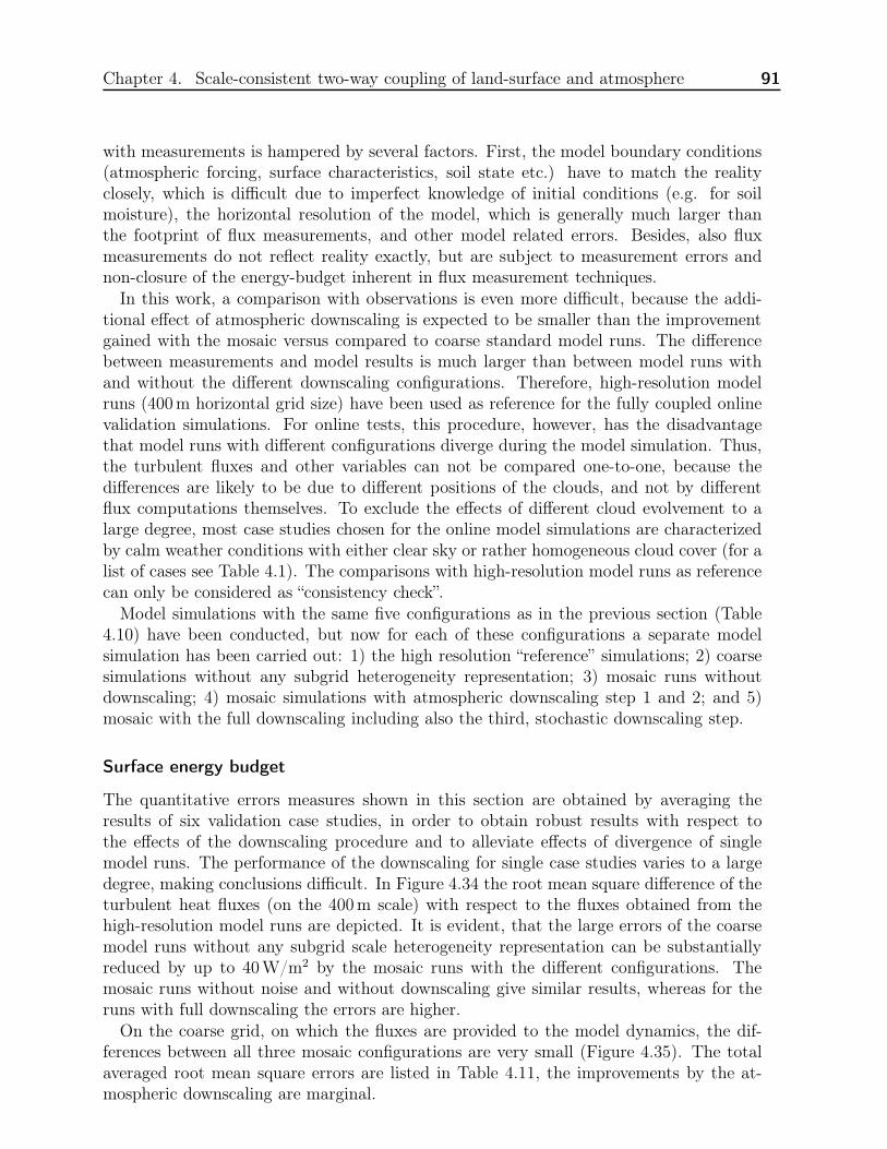
Chapter 4. Scale-consistent two-way coupling of land-surface and atmosphere 91
with measurements is hampered by several factors. First, the model boundary conditions(atmospheric forcing, surface characteristics, soil state etc.) have to match the realityclosely, which is difficult due to imperfect knowledge of initial conditions (e.g. for soilmoisture), the horizontal resolution of the model, which is generally much larger thanthe footprint of flux measurements, and other model related errors. Besides, also fluxmeasurements do not reflect reality exactly, but are subject to measurement errors andnon-closure of the energy-budget inherent in flux measurement techniques.
In this work, a comparison with observations is even more difficult, because the addi-tional effect of atmospheric downscaling is expected to be smaller than the improvementgained with the mosaic versus compared to coarse standard model runs. The differencebetween measurements and model results is much larger than between model runs withand without the different downscaling configurations. Therefore, high-resolution modelruns (400m horizontal grid size) have been used as reference for the fully coupled onlinevalidation simulations. For online tests, this procedure, however, has the disadvantagethat model runs with different configurations diverge during the model simulation. Thus,the turbulent fluxes and other variables can not be compared one-to-one, because thedifferences are likely to be due to different positions of the clouds, and not by differentflux computations themselves. To exclude the effects of different cloud evolvement to alarge degree, most case studies chosen for the online model simulations are characterizedby calm weather conditions with either clear sky or rather homogeneous cloud cover (for alist of cases see Table 4.1). The comparisons with high-resolution model runs as referencecan only be considered as “consistency check”.
Model simulations with the same five configurations as in the previous section (Table4.10) have been conducted, but now for each of these configurations a separate modelsimulation has been carried out: 1) the high resolution “reference” simulations; 2) coarsesimulations without any subgrid heterogeneity representation; 3) mosaic runs withoutdownscaling; 4) mosaic simulations with atmospheric downscaling step 1 and 2; and 5)mosaic with the full downscaling including also the third, stochastic downscaling step.
Surface energy budget
The quantitative errors measures shown in this section are obtained by averaging theresults of six validation case studies, in order to obtain robust results with respect tothe effects of the downscaling procedure and to alleviate effects of divergence of singlemodel runs. The performance of the downscaling for single case studies varies to a largedegree, making conclusions difficult. In Figure 4.34 the root mean square difference of theturbulent heat fluxes (on the 400m scale) with respect to the fluxes obtained from thehigh-resolution model runs are depicted. It is evident, that the large errors of the coarsemodel runs without any subgrid scale heterogeneity representation can be substantiallyreduced by up to 40W/m2 by the mosaic runs with the different configurations. Themosaic runs without noise and without downscaling give similar results, whereas for theruns with full downscaling the errors are higher.
On the coarse grid, on which the fluxes are provided to the model dynamics, the dif-ferences between all three mosaic configurations are very small (Figure 4.35). The totalaveraged root mean square errors are listed in Table 4.11, the improvements by the at-mospheric downscaling are marginal.
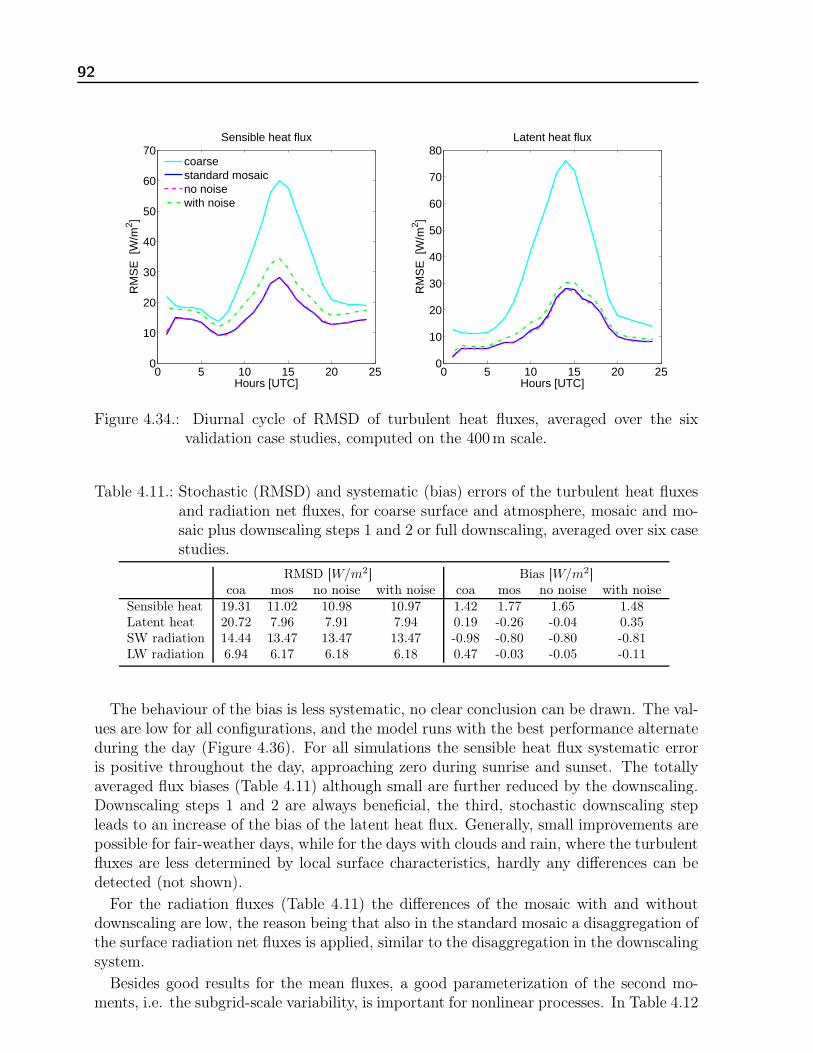
92
0 5 10 15 20 250
10
20
30
40
50
60
70
Hours [UTC]
RM
SE
[W
/m2 ]
Sensible heat flux
coarsestandard mosaicno noisewith noise
0 5 10 15 20 250
10
20
30
40
50
60
70
80
Hours [UTC]
RM
SE
[W
/m2 ]
Latent heat flux
Figure 4.34.: Diurnal cycle of RMSD of turbulent heat fluxes, averaged over the sixvalidation case studies, computed on the 400m scale.
Table 4.11.: Stochastic (RMSD) and systematic (bias) errors of the turbulent heat fluxesand radiation net fluxes, for coarse surface and atmosphere, mosaic and mo-saic plus downscaling steps 1 and 2 or full downscaling, averaged over six casestudies.
RMSD [W/m2] Bias [W/m2]coa mos no noise with noise coa mos no noise with noise
Sensible heat 19.31 11.02 10.98 10.97 1.42 1.77 1.65 1.48Latent heat 20.72 7.96 7.91 7.94 0.19 -0.26 -0.04 0.35SW radiation 14.44 13.47 13.47 13.47 -0.98 -0.80 -0.80 -0.81LW radiation 6.94 6.17 6.18 6.18 0.47 -0.03 -0.05 -0.11
The behaviour of the bias is less systematic, no clear conclusion can be drawn. The val-ues are low for all configurations, and the model runs with the best performance alternateduring the day (Figure 4.36). For all simulations the sensible heat flux systematic erroris positive throughout the day, approaching zero during sunrise and sunset. The totallyaveraged flux biases (Table 4.11) although small are further reduced by the downscaling.Downscaling steps 1 and 2 are always beneficial, the third, stochastic downscaling stepleads to an increase of the bias of the latent heat flux. Generally, small improvements arepossible for fair-weather days, while for the days with clouds and rain, where the turbulentfluxes are less determined by local surface characteristics, hardly any differences can bedetected (not shown).
For the radiation fluxes (Table 4.11) the differences of the mosaic with and withoutdownscaling are low, the reason being that also in the standard mosaic a disaggregation ofthe surface radiation net fluxes is applied, similar to the disaggregation in the downscalingsystem.
Besides good results for the mean fluxes, a good parameterization of the second mo-ments, i.e. the subgrid-scale variability, is important for nonlinear processes. In Table 4.12

Chapter 4. Scale-consistent two-way coupling of land-surface and atmosphere 93
0 5 10 15 20 250
5
10
15
20
25
30
35
40
Hours [UTC]
RM
SE
[W
/m2 ]
Sensible heat flux
coarsestandard mosaicno noisewith noise
0 5 10 15 20 250
10
20
30
40
50
Hours [UTC]
RM
SE
[W
/m2 ]
Latent heat flux
Figure 4.35.: As Fig. 4.34, but computed on the 2.8 km scale.
Table 4.12.: Mean subgrid-scale standard deviations [W m−2], averaged over all six vali-dation case studies.
coa mos no noise with noise ref
Sensible heat 0 12.50 13.30 16.11 13.44Latent heat 0 14.97 14.81 15.65 14.68SW radiation 0 1.85 2.33 5.60 4.96LW radiation 0 2.38 1.64 3.01 2.87
the mean subgrid-scale standard deviations per coarse pixel are listed. For the sensibleheat flux the subgrid scale variability of the mosaic alone is too small, and is increasedto a value closer to the reference if atmospheric downscaling without noise is applied.The heterogeneity of the latent heat flux is too large for the standard mosaic, and can bereduced by the downscaling steps 1 and 2. The full downscaling again leads to excessivevariabilities for both fluxes, probably due to inter-variable relationships not accounted foradequately by the stochastic noise generation. For the radiation fluxes, however, the fulldownscaling gives the best results, because it is trained to parameterize also the effect ofsubgrid-scale variabilities of clouds, while mosaic and mosaic with downscaling step 1 and2 can only account for surface heterogeneities.
Error analysis
In this section the results are analyzed in some more detail, for a better understandingwhy the effect of the downscaling is rather small, even smaller than for the offline testcase in section 4.4.2. Figure 4.37 depicts the root mean square errors for the atmosphericand surface temperature and specific humidity respectively, computed on the 400m scale.The downscaling without noise leads to improved atmospheric temperature of the lowestatmospheric layer (keep in mind that these disaggregated temperatures are only used
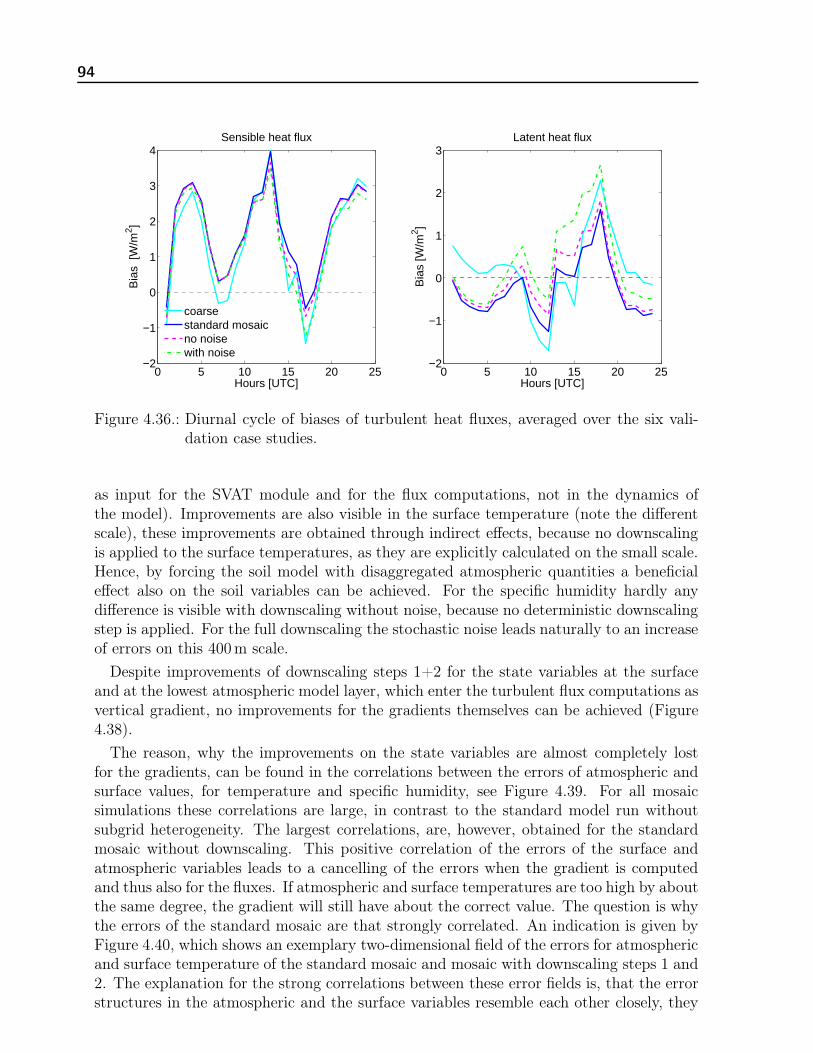
94
0 5 10 15 20 25−2
−1
0
1
2
3
4Sensible heat flux
Hours [UTC]
Bia
s [W
/m2 ]
coarsestandard mosaicno noisewith noise
0 5 10 15 20 25−2
−1
0
1
2
3
Hours [UTC]
Bia
s [W
/m2 ]
Latent heat flux
Figure 4.36.: Diurnal cycle of biases of turbulent heat fluxes, averaged over the six vali-dation case studies.
as input for the SVAT module and for the flux computations, not in the dynamics ofthe model). Improvements are also visible in the surface temperature (note the differentscale), these improvements are obtained through indirect effects, because no downscalingis applied to the surface temperatures, as they are explicitly calculated on the small scale.Hence, by forcing the soil model with disaggregated atmospheric quantities a beneficialeffect also on the soil variables can be achieved. For the specific humidity hardly anydifference is visible with downscaling without noise, because no deterministic downscalingstep is applied. For the full downscaling the stochastic noise leads naturally to an increaseof errors on this 400m scale.
Despite improvements of downscaling steps 1+2 for the state variables at the surfaceand at the lowest atmospheric model layer, which enter the turbulent flux computations asvertical gradient, no improvements for the gradients themselves can be achieved (Figure4.38).
The reason, why the improvements on the state variables are almost completely lostfor the gradients, can be found in the correlations between the errors of atmospheric andsurface values, for temperature and specific humidity, see Figure 4.39. For all mosaicsimulations these correlations are large, in contrast to the standard model run withoutsubgrid heterogeneity. The largest correlations, are, however, obtained for the standardmosaic without downscaling. This positive correlation of the errors of the surface andatmospheric variables leads to a cancelling of the errors when the gradient is computedand thus also for the fluxes. If atmospheric and surface temperatures are too high by aboutthe same degree, the gradient will still have about the correct value. The question is whythe errors of the standard mosaic are that strongly correlated. An indication is given byFigure 4.40, which shows an exemplary two-dimensional field of the errors for atmosphericand surface temperature of the standard mosaic and mosaic with downscaling steps 1 and2. The explanation for the strong correlations between these error fields is, that the errorstructures in the atmospheric and the surface variables resemble each other closely, they

Chapter 4. Scale-consistent two-way coupling of land-surface and atmosphere 95
0 5 10 15 20 250.1
0.2
0.3
0.4
0.5
0.6
Hours [UTC]
RM
SE
[K
]
Temperature
coarsestandard mosaicno noisewith noise
0 5 10 15 20 250
0.5
1
1.5
2
Hours [UTC]
RM
SE
[K
]
Surface temperature
0 5 10 15 20 250
1
2
3
4
5
6x 10
−4
Hours [UTC]
RM
SE
[kg
/kg]
Specific humidity
0 5 10 15 20 250
0.2
0.4
0.6
0.8
1
1.2x 10
−3
Hours [UTC]
RM
SE
[kg
/kg]
Surface specific humidity
Figure 4.37.: Root mean square differences for atmospheric (top) and surface (bot-tom) temperature (left) and specific humidity (right), averaged over all casestudies.
are both caused by the coarse atmospheric forcing in the standard mosaic approach. Over-or underestimations due to unresolved valleys, gradients, or other characteristics are visiblein the atmospheric as well as in the surface temperature field. Some small-scale surfacetemperature structures are captured due to resolved land cover characteristics, however,the edges of the coarse pixels are still visible (see Fig. 4.41). The valleys are too cold,the ridges too warm, which is not the case in the model simulations with disaggregationof the atmospheric forcing variables.
Thus, despite the lower and less structured errors achieved by the downscaling (Fig.4.40 right), this beneficial behaviour does not lead to improvements in the gradients, andtherefore only a marginally better performance is obtained for the fluxes. Contrary to theoffline results, where the subgrid-scale variability of the standard mosaic fluxes is too large,here the reference subgrid-scale standard deviations are matched closely by the standardmosaic approach or are even slightly too low (see Fig. 4.42). Downscaling without noiseleads to a small increase of this variability, which is beneficial during night and for thelatent heat flux, but not during day for the sensible heat flux. Full downscaling leadsgenerally to excessive subgrid-scale variabilities.
A perfect downscaling would still lead to smaller improvements of the mosaic approach

96
0 5 10 15 20 250
0.5
1
1.5
Hours [UTC]
RM
SE
[K
]
Temperature gradient
coarsestandard mosaicno noisewith noise
0 5 10 15 20 250
0.2
0.4
0.6
0.8
1
1.2x 10
−3
Hours [UTC]
RM
SE
[K
]
Humidity gradient
Figure 4.38.: Root mean square differences for temperature (left) and specific humidity(right) gradients between surface and lower atmosphere.
compared to a standard coarse simulation without subgrid-scale heterogeneities. A generalestimate of the effect that can be expected if subgrid heterogeneities on a 400m grid with2.8 km as coarse grid are taken into account can be derived from Figure 4.43. The subgridscale standard deviations at the surface and in the atmosphere are depicted, at nightand during mid-day, for different days with varying weather conditions (for a descriptionof the weather situations see Table 4.1), obtained from 400m model simulations. Forspecific humidity the small-scale variability in the atmosphere is always much lower thanat the surface. For temperature in some nights also large variability is visible in thelower boundary layer, especially for 14 October 2007 and 9 May 2008, both clear nightswithout clouds. During daytime, however, the atmosphere is well mixed, thus subgrid-scale variability is small due to smoothing.
Table 4.13 lists the mean difference between the spatial correlation length of the heatfluxes and the correlation length of the reference 400m simulations. As expected the cor-relation length of the coarse model simulations without subgrid-scale heterogeneity is onaverage too large. For the standard mosaic the correlation length is strongly reduced, andatmospheric downscaling steps one and two further improve the results. The stochasticdownscaling step, however, reduces the spatial autocorrelations too strongly, due to theneglection of spatial correlations.
Effect on model dynamics
The effect on the model dynamics in terms of divergence from the reference has beeninvestigated. In Figure 4.44 the divergence from the high-resolution simulations is shownexemplary for 15 May 2008, for surface pressure, precipitation sum since initializationand 2m temperature, normalized with the respective “reference” standard deviation, toexclude the diurnal cycle. The deviations of the coarse simulation is largest, the threemosaic configurations are closely together, and show a lower divergence from the 400m

Chapter 4. Scale-consistent two-way coupling of land-surface and atmosphere 97
0 5 10 15 20 250
0.1
0.2
0.3
0.4
0.5
0.6
0.7
0.8
Hours [UTC]
Err
or c
orre
latio
n
Temperature
coarsestandard mosaicno noisewith noise
0 5 10 15 20 250
0.1
0.2
0.3
0.4
0.5
0.6
0.7
0.8
Hours [UTC]
Err
or c
orre
latio
n
Specific humidity
Figure 4.39.: Correlations of errors of surface and atmospheric temperature (left) andspecific humidity (right).
]bt[
Table 4.13.: Mean difference of correlation length of sensible and latent heat flux to thecorrelation length of the high-resolution model run. Averaged spatially andtemporally, for all validation case studies, in [m].
coarse mosaic no noise with noise
Sensible heat flux 178.5 36.5 -0.5 -129.0Latent heat flux 156.3 18.10 15.2 -33.9
simulation. The effect of the downscaling, is again rather small.
4.5. Discussion
Interpretation of the results
The performance of the atmospheric downscaling scheme has first been evaluated by ap-plying it to lowest model layer variables of the COSMO model for three case studies. Thefirst two downscaling steps considerably reduce the errors compared to the homogeneouscoarse scale values. All steps increase subgrid-scale variance towards the reference small-scale variability. The first step leads to a small error reduction and a small increase of thesubgrid scale variability. The second step, wherever applicable, largely reduces the errorsand improves variability. Since step 2 is weather dependent, also the performance of thedisaggregation is dependent on the atmospheric conditions. The third step achieves agood reproduction of the subgrid scale variability, however, at the expense of an increasedroot mean square error.
The question remains whether the weak correlations of near surface wind speed and
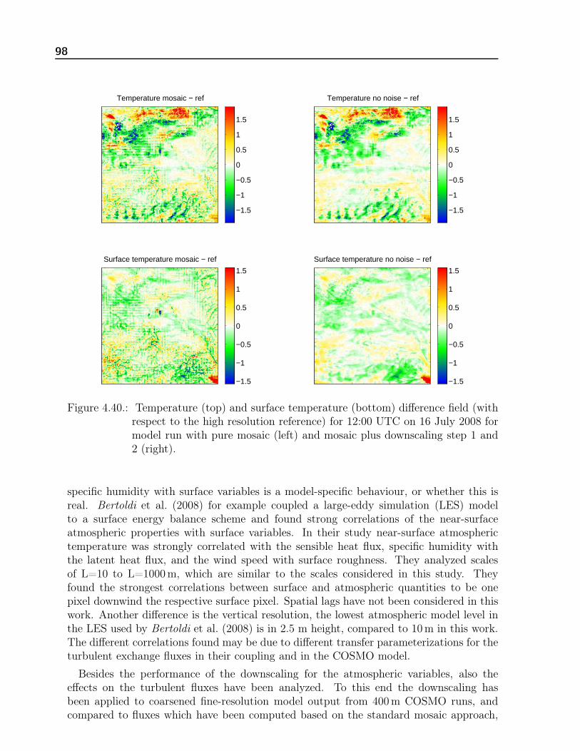
98
Temperature mosaic − ref
−1.5
−1
−0.5
0
0.5
1
1.5
Temperature no noise − ref
−1.5
−1
−0.5
0
0.5
1
1.5
Surface temperature mosaic − ref
−1.5
−1
−0.5
0
0.5
1
1.5
Surface temperature no noise − ref
−1.5
−1
−0.5
0
0.5
1
1.5
Figure 4.40.: Temperature (top) and surface temperature (bottom) difference field (withrespect to the high resolution reference) for 12:00 UTC on 16 July 2008 formodel run with pure mosaic (left) and mosaic plus downscaling step 1 and2 (right).
specific humidity with surface variables is a model-specific behaviour, or whether this isreal. Bertoldi et al. (2008) for example coupled a large-eddy simulation (LES) modelto a surface energy balance scheme and found strong correlations of the near-surfaceatmospheric properties with surface variables. In their study near-surface atmospherictemperature was strongly correlated with the sensible heat flux, specific humidity withthe latent heat flux, and the wind speed with surface roughness. They analyzed scalesof L=10 to L=1000m, which are similar to the scales considered in this study. Theyfound the strongest correlations between surface and atmospheric quantities to be onepixel downwind the respective surface pixel. Spatial lags have not been considered in thiswork. Another difference is the vertical resolution, the lowest atmospheric model level inthe LES used by Bertoldi et al. (2008) is in 2.5 m height, compared to 10m in this work.The different correlations found may be due to different transfer parameterizations for theturbulent exchange fluxes in their coupling and in the COSMO model.
Besides the performance of the downscaling for the atmospheric variables, also theeffects on the turbulent fluxes have been analyzed. To this end the downscaling hasbeen applied to coarsened fine-resolution model output from 400m COSMO runs, andcompared to fluxes which have been computed based on the standard mosaic approach,

Chapter 4. Scale-consistent two-way coupling of land-surface and atmosphere 99
Temperature mosaic
286
288
290
292
294Temperature no noise
286
288
290
292
294
Surface temperature mosaic
285
290
295
300
Surface temperature no noise
285
290
295
300
Figure 4.41.: Temperature (top) and surface temperature (bottom) field for 12:00 UTCon 16 July 2008 for model run with pure mosaic (left) and mosaic plusdownscaling step 1 and 2 (right).
i.e. with a fine surface but coarse atmosphere. The results indicate that improvementsof about 1 W/m2 can be gained by employing the downscaled atmospheric reference levelquantities for the computation of the fluxes, if only downscaling steps 1+2 are carried out.Only during clear-sky radiation nights, with heterogeneous near-surface atmospheres thefull downscaling gives the best results for the sensible heat flux. Contrary to the situationduring daytime, the small-scale variability of the sensible heat flux is too small withoutdownscaling in these situations. The mosaic approach leads to improvements mainly overareas with strong heterogeneity in land use and soil characteristics, whereas the largestpositive effects attributed to the downscaling are on average found over mountainousregions.
Finally, the disaggregation scheme has been implemented into a COSMO model versionwith mosaic surface heterogeneity representation. Comparisons of model output fromsimulations with and without mosaic and downscaling (either steps 1+2 or steps 1+2+3)were carried out. Summarizing, the model simulations with mosaic approach gave overallnotably better results than model simulations without any surface variability representa-tion. Root mean square errors of sensible and latent heat fluxes were reduced by about 9W/m2 and 13 W/m2, respectively (averaged over six case studies).
The new atmospheric downscaling scheme, however, leads to only marginal further

100
0 5 10 15 20 250
5
10
15
20
25
30
35
Hours [UTC]
Sub
grid
−sc
ale
stan
dard
dev
iatio
n [W
/m2 ] Sensible heat flux
0 5 10 15 20 250
10
20
30
40
Hours [UTC]
Sub
grid
−sc
ale
stan
dard
dev
iatio
n [W
/m2 ] Latent heat flux
referencestandard mosaicno noisewith noise
Figure 4.42.: Mean subgrid-scale standard deviation of the sensible (left) and latent(right) heat flux, averaged over the six online validation case studies.
improvements. At first glance, this result is unexpected, because the results for the singleterms in the flux equations mainly show a positive impact. But the gradients and thusthe fluxes do not benefit from this effect. The cause for this behaviour can be foundin the characteristics of the errors. For the standard mosaic the errors of surface andatmospheric temperature (and also to some degree for specific humidity) are strongercorrelated. Thus, if the temperature at the atmospheric reference level is too high, ingeneral also the surface is too warm. This leads to a cancelling of errors of the fluxes inthe standard mosaic approach. Thus, although the structure of the surface variables ismore realistic due to the distributed atmospheric forcing, the overall benefits are marginal.
In the offline computation of the fluxes this effect is not visible, because the surface fieldsin the offline tests were the same for the standard mosaic offline flux as well as for themosaic with atmospheric downscaling, namely high-resolution model output. The simplesetup does not allow the simulation of feedback processes, hence it can only reveal partof the behaviour of the fully coupled model system. The offline evaluation can howeverbe regarded as proof of concept for applications of the disaggregation for stand-alone soilmodel applications.
To outperform the standard mosaic approach an option would be to downscale thegradients directly, instead of the screen-level parameters. This, however, is much moredifficult, because clear physical relations with surface quantities do not exist.
Generally the stochastic downscaling step, does not improve the results. Although theadded small-scale variability has about the right value for each of the downscaled variables,the variability for the fluxes is too large, indicating more not-captured cross-correlationsbetween the relevant variables.
The additional effects, which can be expected due to the disaggregation of the at-mospheric forcing variables, are much smaller than those of the mosaic approach versusmodel simulations without surface heterogeneity representation, because the surface ismuch more heterogeneous than the atmosphere. Only during clear-sky nights the near-

Chapter 4. Scale-consistent two-way coupling of land-surface and atmosphere 101
0 0.5 1 1.50
500
1000
1500
[K]
Hei
ght [
m]
Mean stddev of anomalies Tpot 4:00 UTC
27 Aug 200714 Oct 20073 Mar 20081 May 20089 May 2008
0 2 4 6 8
x 10−4
0
500
1000
1500
[kg/kg]
Hei
ght [
m]
Mean stddev of anomalies QV 4:00 UTC
0 0.5 1 1.5 20
500
1000
1500
[K]
Hei
ght [
m]
Mean stddev of anomalies Tpot 12:00 UTC
0 0.5 1 1.5
x 10−3
0
500
1000
1500
[kg/kg]
Hei
ght [
m]
Mean stddev of anomalies QV 12:00 UTC
Figure 4.43.: Subgrid-scale standard deviations for potential temperature (left) and spe-cific humidity (right) for 4:00 (top) and 12:00 UTC (bottom) in the atmo-sphere and at the surface (marked by crosses).
surface atmospheric temperature variability is comparably large, but still only half aslarge as the mean surface heterogeneity.
Surface heterogeneity representation in general is most important in calm weather sit-uations. In synoptically driven weather conditions with strong advection, or large-scalerainfall or cloud cover, the surface characteristics have less impact on the surface fluxesand lower boundary layer. It is believed that the coupling strength (i.e. the degree towhich anomalies in land-surface state can affect rainfall generation and other atmosphericprocesses; Koster et al., 2006) between surface and atmosphere is strongest in summer,when the evapotranspiration rates are high.
Scales
There are a few studies where atmospheric disaggregation in combination with the mosaicapproach has been applied (e.g. Seth et al., 1994; Giorgi et al., 2003; Dimri , 2009, for anoverview refer to section 4.1). In these studies positive effects due to e.g. temperaturedownscaling have been demonstrated. Their simulations however were conducted on scalesof about 50-100 km for several months or even years, and over highly structured terrain
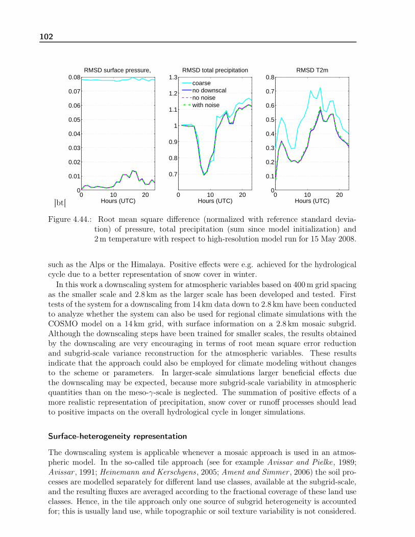
102
]bt[0 10 20
0
0.01
0.02
0.03
0.04
0.05
0.06
0.07
0.08RMSD surface pressure,
Hours (UTC)0 10 20
0.7
0.8
0.9
1
1.1
1.2
1.3
Hours (UTC)
RMSD total precipitation
coarseno downscalno noisewith noise
0 10 200
0.1
0.2
0.3
0.4
0.5
0.6
0.7
0.8RMSD T2m
Hours (UTC)
Figure 4.44.: Root mean square difference (normalized with reference standard devia-tion) of pressure, total precipitation (sum since model initialization) and2m temperature with respect to high-resolution model run for 15 May 2008.
such as the Alps or the Himalaya. Positive effects were e.g. achieved for the hydrologicalcycle due to a better representation of snow cover in winter.
In this work a downscaling system for atmospheric variables based on 400m grid spacingas the smaller scale and 2.8 km as the larger scale has been developed and tested. Firsttests of the system for a downscaling from 14 km data down to 2.8 km have been conductedto analyze whether the system can also be used for regional climate simulations with theCOSMO model on a 14 km grid, with surface information on a 2.8 km mosaic subgrid.Although the downscaling steps have been trained for smaller scales, the results obtainedby the downscaling are very encouraging in terms of root mean square error reductionand subgrid-scale variance reconstruction for the atmospheric variables. These resultsindicate that the approach could also be employed for climate modeling without changesto the scheme or parameters. In larger-scale simulations larger beneficial effects duethe downscaling may be expected, because more subgrid-scale variability in atmosphericquantities than on the meso-γ-scale is neglected. The summation of positive effects of amore realistic representation of precipitation, snow cover or runoff processes should leadto positive impacts on the overall hydrological cycle in longer simulations.
Surface-heterogeneity representation
The downscaling system is applicable whenever a mosaic approach is used in an atmos-pheric model. In the so-called tile approach (see for example Avissar and Pielke, 1989;Avissar , 1991; Heinemann and Kerschgens, 2005; Ament and Simmer , 2006) the soil pro-cesses are modelled separately for different land use classes, available at the subgrid-scale,and the resulting fluxes are averaged according to the fractional coverage of these land useclasses. Hence, in the tile approach only one source of subgrid heterogeneity is accountedfor; this is usually land use, while topographic or soil texture variability is not considered.
Chapter 4. Scale-consistent two-way coupling of land-surface and atmosphere 103
The approach presented here cannot be applied without modifications to a tiled surface,because high-resolution surface information of different surface properties is necessary, forexample of topographic height, albedo and surface temperature. This usually is availablein a consistent way only in the explicit subgrid mosaic approach.
A general drawback of both mosaic and tile approach is the neglect of horizontal fluxesand advective effects between patches within a grid box. If for example a cool water bodyis situated upwind of an agricultural sub-pixel, in reality the atmospheric conditions atthe downstream pixels would be affected by advection of cool or moist air, and thus alsothe turbulent fluxes.
Soil moisture
A general issue, which has not been discussed in this study, is soil moisture initialization.Many studies show the strong dependence of simulated fluxes on the soil moisture rep-resentation (e.g. Chow et al., 2006; Maxwell et al., 2007; Schmidli et al., 2009), at leastunder calm weather conditions. In this work the soil moisture has been initialized byinterpolating soil moisture from COSMO-DE analyses, also for the 400m model simula-tions. Inadequately represented soil moisture fields can lead to a biased partitioning ofthe available energy into sensible and latent heat. For the development of the atmos-pheric downscaling system, however, the accurate soil moisture representation was notcrucial, because for that purpose a close representation of “real” conditions was not im-portant, only the consistent modeling of the inter-variable relations. In an operationalemployment of the mosaic approach, high-resolution soil initialization information wouldbe available, stored on the subgrid from the previous model runs. Generally, the appli-cation of the mosaic in a continuous data-assimilation-forecast system is preferred overthe single case studies carried out in this work, because then spin-up effects due to coarsesoil-initialization would cease to exist.
Potential applications
Possible applications of the downscaling scheme are the generation of high-resolutioninput for SVAT models and hydrological models, based on low-resolution atmosphericmodel output. This can be useful for either stand-alone applications, or for fully coupledsimulations, where the soil is resolved on a finer grid than the atmosphere. A largebeneficial effect of a mosaic in combination with the atmospheric disaggregation should beexpected for applications in highly structured terrain, for example in the Alpine region, dueto a more realistic partitioning of precipitation in rain and snow dependent on elevationleading to indirect positive impacts due to more realistic patterns of high and low surfacealbedo over snow-covered and snow-free subpixels.
Another application would be the modeling of fog. The simulation of fog-formationrequires an accurate simulation of the feedbacks between surface and atmosphere. Bothtemperature and specific humidity in the lower boundary need to be captured accurately.Such a setup would allow running a fog model on the higher mosaic resolution.
Since COSMO model version 3.18, a lake parameterization (FLake, Mironov et al., 2010)is available (although not operationally used) in the COSMO model. This module is abulk model capable of predicting the vertical temperature structure and mixing conditions
104
at various depth of inland water bodies, and thus to represent the effects of lakes onnumerical weather prediction models. The implementation could be modified to allow asubgrid application of this FLake model in the mosaic with atmospheric disaggregation.That way also effects of lakes smaller than the horizontal grid resolution could be takeninto account.
Neunhäuserer et al. (2007) simulated urban heat island effects with COSMO on a 1.1 kmgrid for Helsinki by introducing urban external surface parameters and an anthropogenicheat source (introduced into the surface heat budget equation). A mosaic representationcould take into account the effects of small cities in model simulations with coarser meshsizes.
The downscaling scheme should be tested in combination to hydrological models byproviding high-resolution atmospheric input for these models. Using atmospheric modeloutput directly to drive hydrological models can lead to too low precipitation intensities,attributed to the generally too low spatial resolution of atmospheric models, comparedto hydrological models. Too low precipitation rates can give rise to unrealistic low runoff(see, e.g., Segond et al., 2007).
Possible improvements
In the future, attempts should be made to conserve also spatial correlations in downscalingstep 3, i.e. to generate spatially red noise instead of white noise. This would be especiallyimportant for distributed hydrological models, which are usually three-dimensional modelsand simulate lateral exchange.
The mosaic approach in the version implemented in the COSMO-SUBS model versioncontains the subgrid approach only for the turbulent fluxes of sensible and latent heat,whereas the momentum flux is still calculated on the coarse scale. The reason for thisinconsistent treatment is that in COSMO the roughness length z0 contains not only theroughness of the land cover characteristics, but also a second term for gravity wave dragfor the momentum flux computations. The latter part can not be readily disaggregated inthe current implementation. In a newer COSMO model version, a new, separate parame-terization of this gravity wave drag, after Lott and Miller (1997), has been implemented.For application of the mosaic in a more recent COSMO model version, a mosaic-typeimplementation also for the momentum flux should be developed.
Another important topic is validation. The offline computation of the fluxes does notrepresent the effects in a coupled model system, and can thus only help to understand theeffects of the system. Online validation by comparing the different mosaic and downscalingconfigurations with high-resolution reference model simulations, however, is hamperedby divergence of the model simulations. The high-resolution simulations can only beused as consistency check and proof of concept, not as the “true” atmospheric state.As a compromise between these two test environments a test with a stand-alone SVATmodule would provide another testbed, for example TERRA stand-alone. That waythe soil module could be run on high resolution, to emulate the mosaic approach, andcould be driven by either high-resolution (as reference), coarse (as standard mosaic), ordisaggregated (as test of the downscaling) atmospheric information. Thus, the effectsof the downscaling could be isolated more easily, effects of different cloud positions forexample could be excluded. Furthermore, longer simulations would be possible. However,

Chapter 4. Scale-consistent two-way coupling of land-surface and atmosphere 105
also in such a setting no feedbacks between the soil-vegetation system and atmospherecan be considered and conclusions concerning effects of the scale-consistent soil-vegetation-atmosphere coupling on the atmospheric model evolution would not be possible.


5. Concluding remarks
A detailed discussion of the two presented approaches have been given at the end ofthe respective chapters. In this chapter more general conclusions with respect to bothintroduced schemes are drawn and possible future research topics are sketched.
Novelty and goals of the proposed techniques
In this work two approaches have been presented, which aim at an adequate and effi-cient representation of small-scale heterogeneities in numerical weather prediction mod-els. Heterogeneity in the atmosphere is accounted for with respect to radiative transferby a computationally efficient approach that is able to track small fast moving clouds.Heterogeneity at the surface is accounted for by computing the soil-surface-vegetation pro-cesses on a higher horizontal resolution, including a novel downscaling scheme to generatespatially distributed small-scale atmospheric forcing.
The appropriate consideration of heterogeneities becomes more important with decreas-ing grid sizes of the atmospheric models, because the processes are less Gaussian on smallscales and inherent nonlinearities hamper the use of averaged and effective parameters.The available computer time is, however, always a constraining factor. This leads to thepractise to use spatial and temporal sampling and averaging techniques for the compu-tation of physical processes in operational meteorological models. The two approachesintroduced in this work provide solutions to overcome these neglections of small-scalevariability and thus represent patterns in the soil-vegetation-atmosphere system moreadequately.
Both, a better representation of radiative effects and a scale-consistent coupling of land-surface and atmosphere, lead to an improved energy budget at the earth surface, whichis crucial as the lower boundary for the atmospheric model and has a large impact onboundary layer development.
A new aspect is the explicit estimation and generation of subgrid-scale variability byadding random noise, which has been introduced in the downscaling scheme. In thepast, parameterizations have typically been used to predict the evolution of grid-meanquantities due to unresolved subgrid-scale processes. In recent years, however, the fieldof stochastic modeling (Palmer and Williams, 2009) has evolved, which moves away frombulk formula parameterizations towards the incorporation of stochastic terms in climateand weather forecast models, in order to account for the uncertainty inherent in thesubgrid-scale processes. Such stochastic representations of subgrid-scale processes arealso valuable to account for model error in ensemble systems, (see e.g. Buizza et al., 1999)and the stochastic step in the downscaling scheme can be considered as an application ofthis theory.
107

108
Critical assessment of the results
Both schemes, the adaptive radiation scheme and the atmospheric downscaling in com-bination with the mosaic approach, have been implemented into the COSMO model andtest cases have been simulated for the COSMO-DE configuration on a horizontal gridresolution of 2.8 km.
By employing the adaptive radiative transfer parameterization error reductions by 15-25 % for the radiation surface net fluxes compared to the COSMO-DE default radiationsetup were achieved. Model consistency was improved by a more realistic simulation ofthe relation of cloud characteristics and radiation. Furthermore, it was demonstrated thatmodel runs with the adaptive radiation diverge less from the reference model run.
The improvements gained by the combination of the mosaic approach with atmosphe-ric disaggregation have to be considered more differentiated. It has been proven that theincorporation of surface heterogeneity into the COSMO model has a large positive impact(as shown before by Ament and Simmer , 2006), reducing the root mean square differ-ences of the fluxes to reference high-resolution simulations by about 50%. The additionalintroduction of subgrid-scale atmospheric forcing for the sub-pixels by statistical down-scaling, however, led only to marginal additional improvements, although the downscalingitself works well. The rather small effect can be explained by two factors: First, it hasbeen shown that the atmosphere is less heterogeneous, especially on theses small scales,compared to the soil surface. Second, in the standard mosaic approach with homoge-neous atmospheric forcing, errors for the surface and atmospheric variables are stronglypositively correlated, i.e. overestimations in e.g. atmospheric temperature coincides withoverestimation in surface temperature (and vice versa), which leads to a cancellation oferrors. Thus, although the downscaling leads to more realistic fields of surface and near-surface variables, the net effect on the turbulent fluxes is less pronounced. This, however,is due to the rather simple parameterization of the exchange fluxes in current atmosphericmodels. In future applications, especially on smaller scales, non-local effects may becomemore important, and thus the fluxes will likely be parameterized by other, less simpleconcepts than after Monin-Obukhov. Then a realistic representation of the fields willprobably prove valuable.
In conclusion, the operational application of the adaptive radiation parameterizationcan be recommended, because it has a large positive impact and does not lead to anincrease in computation time. The mosaic approach itself also leads to a considerableimprovement for the representation of the turbulent heat fluxes, and the whole dynamicalmodel development. Thus, an operational employment of the mosaic approach should alsobe considered, although the higher resolution of the soil module lead to higher computa-tional demands, depending on the subgrid resolution. In this work a subgrid resolutionof 7x7, i.e. of 49 sub-pixels per coarse pixel, has been used. A sensitivity study chang-ing the number of sub-pixels and evaluating the tradeoff between lower errors versusincreased computing time should be carried out, to find an optimal compromise for anoperational application. Due to the small overall effect of the atmospheric disaggregationon the model simulation an operational application can not necessarily be recommended.The disaggregation approach, however, is computationally cheap, and does thus not in-crease computation time noticeably. And although the effects for meteorological modelsare rather small in the current setup, a positive impact can be expected if hydrologi-

Chapter 5. Concluding remarks 109
cal models are driven with distributed atmospheric forcing generated by the atmosphericdownscaling scheme. A more realistic structure of precipitation and the other atmosphe-ric driving variables will lead to an improved soil moisture distribution. Also a positiveeffect on runoff can be expected, especially in convective situations with heterogeneousprecipitation patterns.
Other aspects of physical parameterizations in numerical atmospheric models wouldbe more worthwhile to invest in, because larger beneficial effects could be expected. Forexample, Ament (2006) showed that a measurement driven soil moisture analysis andimprovements in the SVAT scheme TERRA such as using enhanced stomatal resistanceparameters, had a larger positive effect than the representation of subgrid-scale hetero-geneities. Another topic neglected in most atmospheric models is ground water depth.Maxwell et al. (2007) and Kollet and Maxwell (2008) showed that the effects of variationsin ground water depth on latent heat flux may be as large as effects due to variationsin soil type and land use, if the groundwater level is in the range of a critical depth,i.e. not too far away from the surface, but also not too shallow. Especially under calmconditions the development of the atmospheric boundary layer is strongly influenced bythe available soil water. Thus, the efforts in improving the description of the soil surfacestate should not be constrained to constant parameters such as land cover representation.Advancements in soil moisture assimilation and parameterization techniques are highlydesirable, though challenging. Optimal would be a representation of lateral surface andsubsurface flow, to simulate e.g. topographic effects on soil ground water and soil wateravailability adequately.
A drawback of both introduced methods in this work is that they both contain severalempirically and statistically derived parameters, for example the search algorithm in theadaptive radiation scheme, and the regression coefficients in the regression based down-scaling rules. Generally, parameterizations, which are mainly based on physical equationsand less on tunable parameters, are desirable, as they are more easily transferable toother scales, climates or other applications than the special application for which theywere trained. This, however, is a general problem of parameterizations which provide anestimate of the effect of subgrid-scale processes on grid-scale variables.
Possible aspects of future work
Both schemes should be tested on other scales than the meso-γ-scale. The adaptiveradiation scheme has already been proven to yield good results for the COSMO-EU con-figuration with a horizontal grid mesh size of 7 km (section 3.4.2). For small scales anadequate sampling of fast developing and advection clouds is more important, than onlarger scales on which the cloud cover is more homogeneous. Nevertheless benefits dueto a more frequent sampling than the infrequent calls to the radiation scheme, as usuallyperformed in global models, are possible. In section 4.4.1 it has been shown that thedownscaling gives also satisfactory results for disaggregating the atmospheric variablesfrom a 14 km horizontal grid size to 2.8 km, which would be a possible application of themosaic in regional climate simulations. However, online tests of this setting have notyet been carried out. On that scale, possibly larger effects than in this work could beexpected, because more subgrid-scale heterogeneity is neglected on the regional climatescale. According to the same arguments, also an employment in global models would be

110
advisable, though computational resources have to be taken into consideration.A general issue is the evaluation of the model simulations including one or both of the
presented techniques. In this work validation has been limited to comparisons with eitherhigher resolution model simulations (for the mosaic/downscaling model runs), more as aconsistency check, or simulations with high-frequent radiation computations (for the adap-tive radiation parameterization validation). For a profound validation, a large number ofsimulations, ideally in a continuous data-assimilation-forecast-cycle should be carried outand detailed comparisons should be made in an operational verification framework, to beable to draw final conclusions about the performance in operational numerical weatherprediction systems.
In this work the two new techniques with respect to radiation and soil/surface param-eterizations have been tested separately. As a next step an combined implementation ofthese two schemes into the actual COSMO model version and test cases with applicationof both, the adaptive radiation scheme and better resolved soil module including down-scaling, could be evaluated. One application for which a combination of both techniqueswould be beneficial, is the consideration of topographical effects in the radiation module.During sunrise and sunset, shading and increased solar insolation absorption to slope in-clination is important, as it strongly influences the local surface heat budget. Thermalsurface contrasts resulting from slope orientation can have a large impact on turbulentfluxes and local flow (Seth et al., 1994), because the orientation of the terrain with respectto the sun is a critical parameter for capturing the right amount of solar insulation at thesurface (Avissar and Pielke, 1989). Chow et al. (2006) for example demonstrated thatthe consideration of topographic shading in the radiation module can delay the breakupof the morning inversion layer by about half an hour and impact the valley and slopewind patterns strongly. The adaptive radiation parameterization leads to a better rep-resentation of the surface radiation net fluxes during sunrise and sunset due to a bettersampling and due to the correction of the fluxes according to actual solar zenith angle.Spatial variability in direct solar insulation due to terrain slope, aspect and shading couldbe captured adequately on the high surface resolution in the mosaic approach, thus herea combination of the adaptive radiation and scale-consistent land surface modeling mayresult in a large positive impact. The option for topographical corrections in the radiationscheme is available in the COSMO model since model version 3.23. Thus, such a studywould be straightforward in principle, however the respective external parameters wouldhave to have be prepared first.
Another promising idea would be the development of an adaptive framework for otherparts of the model physics. A possible extension could be the coupling of the existingmodel system with a hydrological model, where the hydrological model is called in onlya fraction of time or space with an intelligent sampling and with a generalization to therest of the field in other timesteps.

A. List of Abbreviations
Acronym Explanation
CCA Canonical Correlation AnalysisCFL Courant-Friedrichs-LeviCLM Community Land ModelCORINE CoORdination of INformation on the EnvironmentCOSMO COnsortium for SMall-scale MOdelingCOSMO-DE COSMO-model DEutschlandCOSMO-EU COSMO-model EUropeDEM Digital Elevation ModelDWD German Weather Service (Deutscher Wetterdienst)ECMWF European Centre of Medium-range Weather ForecastsFAO Food and Agriculture Organization of the United NationsGCM Global Circulation ModelGME Global model of the DWDIFS Integrated Forecasting SystemLAI Leaf area indexLES Large Eddy SimulationLITFASS Lindenberg Inhomogeneous Terrain - Fluxes between
Atmosphere and Surface - a long term StudyLM Lokal-Modell (former name of COSMO model)LLM LITFASS-Lokal-ModellLMK Lokal-Modell KürzestfristLW LongwaveLWP Liquid Water PathMODIS MODerate-resolution Imaging SpectroradiometerPCA Principal Component AnalysisPDF Probability Density FunctionSRTM Shuttle Radar Topography MissionSVAT Soil Vegetation Atmosphere TransferSW ShortwaveTKE Turbulent kinetic energyUNESCO United Nations Educational, Scientific and Cultural OrganizationUTC Universal Time Coordinated
111


B. List of Symbols
Symbol Definition
c specific heat capacityCLC cloud coverCLC2
var cloud cover variance of 3x3 coarse neighboring pixelsDD wind directionDw hydraulic diffusivityEb evaporation of bare soilEi evaporation from interception storeEpot potential evaporationEsnow evaporation from snow store(Fqv)sfc surface flux of water vapor(Fh)sfc sensible heat fluxFRland fraction of landFwl
flux of soil water ψFψ flux of variable ψfi fractional coverage of grid box by interception waterfplnt fraction of grid box covered by vegetationfsnow snow covered fraction of grid boxfψ forcing term due to slow processesGP heat flux of freezing rain and melting snowfallGsnow,melt heat flux of melting surface snowGψ nudging coefficientGsfc soil heat flux at surfaceH orographyKψ threedimensional turbulence coefficient of variable ψKh transfer coefficient for heatKw hydraulic conductivityk vertical indexkesoil number of vertical soil layersLAI leaf area indexL latent heat of vaporizationLnet longwave net radiation flux at surfaceLWP liquid water pathPREC precipitation (rain, snow, graupel)PS surface pressurePψ all dynamic and physical processes of the modelQrad,net net radiation at the surface
113

114
Qv saturation specific humidityqc cloud waterqi cloud iceqg graupelqr rain waterqs specific snow water contentqv specific humidityqvgr25 specific humidity gradient of lowest 2 layers (25 meters)qvgr60 specific humidity gradient of lowest 3 layers (60 meters)qvgr105 specific humidity gradient of lowest 4 layers (105 meters)qvsfc specific humidity at surface(qvsfc)var variance of 3x3 neighboring pixels of surface specific humidityRH near-surface relative humiditySnet shortwave net radiation flux at surfacesψ source terms due to fast processes (sound and gravity waves)T temperatureTG ground temperatureTgr25 temperature gradient of lowest 2 layers (25 meters)Tgr60 temperature gradient of lowest 3 layers (60 meters)Tgr105 temperature gradient of lowest 4 layers (105 meters)Tsfc surface temperatureTso soil temperatureTr transpirationU near-surface u-wind componentV near-surface v-wind componentWso soil moisture of top soil layervh horizontal wind vectorWk weight in nudging system between 0 and 1wl liquid water fraction: liquid water content per layer of thickness ∆zz vertical coordinatez0 roughness lengthαso solar albedoαIR infrared albedoζ vertical orography following coordinateλ heat conductivityρ air densityρw water densityψ arbitrary atmospheric variableσ Stefan-Boltzmann-constantΘ solar zenith angle

Bibliography
Ament, F., Energy and moisture exchange processes over heterogeneous land-surfaces ina weather prediction model , Ph.D. thesis, Rheinische Friedrich-Wilhelms-UniversitätBonn, 2006.
Ament, F. and C. Simmer, Improved representation of land-surface heterogeneity in anon-hydrostatic numerical weather prediction model, Bound. Layer Meteorol., 121, 1,153–174, 2006.
Arola, A., Parameterization of turbulent and mesoscale fluxes for heterogeneous surfaces,J. Atmos. Sci., 56, 584–598, 1999.
Avissar, R., A statistical-dynamical approach to parameterize subgrid-scale land-surfaceheterogeneity in climate models, Surv. Geophys., 12, 155–178, 1991.
Avissar, R., Conceptual aspects of a statistical-dynamical approach to represent landscapesubgrid-scale heterogeneities in atmospheric models, J. Geophys. Res., 97, 2729–2741,1992.
Avissar, R., Which type of soil-vegetation-atmosphere transfer scheme is needed for generalcirculation models: a proposal for a higher-order scheme, J. Hydrology , 212-213, 136–154, 1998.
Avissar, R. and R. A. Pielke, A parameterization of heterogeneous land surfaces for at-mospheric numerical models and its impact on regional meteorology, Mon. Wea. Rev.,117, 2113–2136, 1989.
Avissar, R. and T. Schmidt, An evaluation of the scale at which ground-surface heat fluxpatchiness affects the convective boundary layer using large-eddy simulations, J. Atmos.Sci., 55, 2666–2689, 1998.
Baldauf, M., J. Förstner, S. Klink, T. Reinhardt, C. Schraff, A. Seifert, and K. Stephan,Kurze Beschreibung des Lokal-Modells Kürzestfrist COSMO-DE (LMK) und seinerDatenbanken auf dem Datenserver des DWD, Deutscher Wetterdienst, GeschäftsbereichForschung und Entwicklung, Offenbach, Germany, http://www.cosmo-model.org, 2009.
Bardossy, A., I. Bogardy, and I. Matyasovszky, Fuzzy rule-based downscaling of precipi-tation, Theor. Appl. Climatol., 23, 11–22, 2005.
Bardossy, A., J. Stehlik, and H.-J. Caspary, Automated objective classification of dailycirculation pattens for precipitation and temperature downscaling based on optimizedfuzzy rules, Climate Res., 23, 11–22, 2002.
115

116
Barker, H. W., G. L. Stephens, and Q. Fu, The sensitivity of domain-averaged solar fluxesto assumptions about cloud geometry, Q. J. R. Meteorol. Soc., 125, 2127–2152, 1999.
Benestad, R. E., I. Hanssen-Bauer, and D. Chen, Empirical-Statistical Downscaling , WorldScientific Publishing Co. Pte. Ltd., 2008.
Bertoldi, G., W. P. Kustas, and J. D. Albertson, Estimating spatial variability in at-mospheric properties over remotely sensed land surface conditions, J. Appl. Meteor.Climatol., 47, 2147–2165, 2008.
Beyrich, F., J. Leps, M. Mauder, J. Bange, T. Foken, S. Huneke, H. Lohse, A. Lüdi,W. Meijninger, D. Mironov, U. Wesensee, and P. Zittel, Area-averaged surface fluxesover the LITFASS region based on eddy-coveriance measurements, Bound. Layer Me-teorol., 121, 33–65, 2006.
Beyrich, F. and H.-T. Mengelkamp, Evaporation over a heterogeneous land surface:EVA_GRIPS and the LITFASS-experiment - an overview, Bound. Layer Meteorol.,121, 5–32, 2006.
Bindlish, R. and A. P. Barros, Disaggregation of rainfall for one-way coupling of atmos-pheric and hydrological models in regions of complex terrain, Global and PlanetaryChange, 25, 111–132, 2000.
Boé, J., L. Terray, F. Habets, and E. Martin, Statistical and dynamical downscaling ofthe Seine basin climate for hydro-meteorological studies, Int. J. Clim., 27, 1643–1655,2007.
Bonan, G. B., D. Pollard, and S. L. Thompson, Influence of Subgrid-Scale Heterogene-ity in Leaf Area Index, Stomatal Resistance, and Soil Moisture on Grid-Scale Land-Atmosphere Interactions, J. Climate, 6, 1882–1896, 1993.
Brussolo, E., J. von Hardenberg, L. Ferraris, N. Rebora, and A. Provenzale, Verificationof Quantitative Precipitation Forecasts via Stochastic Downscaling, J. Hydrometeo., 9,1084–1094, 2008.
Brussolo, E., J. von Hardenberg, and N. Rebora, Stochastic versus Dynamical Downscal-ing of Ensemble Precipitation Forecasts, J. Hydrometeo., 10, 1051–1061, 2009.
Buizza, R., M. Miller, and T. N. Palmer, Stochastic representation of model uncertaintiesin the ECMWF ensemble prediction system, Q. J. R. Meteorol. Soc., 125, 2887–2908,1999.
Chevallier, F., F. Chéruy, N. A. Scott, and A. Chédin, A neural network approach for afast and accurate computation of a longwave radiative budget, J. Appl. Meteorol., 37,1385–1397, 1998.
Chevallier, F., J.-J. Morcrette, F. Chéruy, and N. A. Scott, Use of a neural-network-based long-wave radiative-transfer scheme in the ECMWF atmospheric model, Q. J.R. Meteorol. Soc., 126, 761–776, 2000.
Bibliography 117
Chow, F., A. Weigel, R. Street, M. Rotach, and M. Xue, High-resolution large-eddysimulations of flow in a steep Alpine valley. part i: Methodology, verification, andsensitivity experiments, J. Appl. Meteor. Climatol., 45, 63–86, 2006.
Claussen, M., Estimation of areally-averaged surface fluxes, Bound. Layer Meteorol., 54,387–410, 1991.
Claussen, M., Flux aggregation at large scales: on the limits of validity of the concept ofblending height, J. Hydrology , 166, 371–382, 1995.
Clough, S., M. Shephard, E. Mlawer, J. Delamere, M. Iacono, K. Cady-Pereira, S. Bouk-abara, and P. Brown, Atmospheric radiative transfer modeling: A summary of the AERcodes, J. Quant. Spectrosc. Radiat. Transfer , 91, 233–244, 2005.
Cox, P., R. Betts, C. Bunton, R. Essery, P. Rowntree, and J. Smith, The impact of newland surface physics on the GCM simulation of climate and climate sensitivity, ClimateDyn., 15, 183–203, 1999.
de Rooy, W. C. and K. Kok, A combined physical-statistical approach for the downscalingof model wind speed, Wea. Forecasting , 19, 485–495, 2004.
Dickinson, R., Modeling evapotranspiration for three-dimensional global climate models:Climate processes and climate sensitivity, Geophysical Monograph 29 , 5, 58–72, 1984.
Dickinson, R., A. Henderson-Sellers, and P. Kennedy, Biosphere atmosphere transferscheme (BATS) version 1e as coupled to the NCAR Communtiy Climate Model, NCARTech. Note NCAR/TN-387-STR, Natl. Cent. for Atmos. Res. Boulder Colorado, 1993.
Dimri, A., Impact of subgrid scale scheme on topography and landuse for better regionalscale simulation of meteorological variables over the western himalayas, Clim. Dyn., 32,565–574, 2009.
Doms, G., J. Förstner, E. Heise, H.-J. Herzog, M. Raschendorfer, T. Reinhardt, B. Rit-ter, R. Schrodin, J.-P. Schulz, and G. Vogel, A description of the nonhydrostatic re-gional model LM, Part II: Physical parameterization, Deutscher Wetterdienst, P.O. Box100465, 63004 Offenbach, Germany, 2007.
EEA, Corine Land Cover (CLC90), European Environment Agency, Copenhagen DK,2000, http://dataservice.eea.eu.int/dataservice/.
Essery, R., M. Best, R. Betts, and P. Cox, Explicit representation of subgrid heterogeneityin a GCM land surface scheme, J. Hydrometeo., 4, 530–543, 2003.
Farr, T. G., P. A. Rosen, E. Caro, R. Crippen, R. Duren, S. Hensley, M. Kobrick, M. Paller,E. Rodriguez, L. Roth, D. Seal, S. Shaffer, J. Shimada, J. Umland, M. Werner, M. Oskin,D. Burbank, and D. Alsdorf, The shuttle radar topography mission, Rev. Geophys., 45,2007, doi: 10.1029/2005RG000183.
Früh, B., J. Schipper, A. Pfeiffer, and V. Wirth, A pragmatic approach for downscalingprecipitation in alpine-scale complex terrain, Meteorol. Z., 15, No. 6, 631–646, 2006.

118
Gao, Y., F. Chen, M. Barlage, W. Liu, G. Cheng, X. Li, Y. Yu, Y. Ran, H. Li, H. Peng,and M. Ma, Enhancement of land surface information and its impact on atmosphericmodeling in the heihe river basin, northwest china, J. Geophys. Res., 113, D20S90,2008.
Giorgi, F. and R. Avissar, Representation of heterogeneity effects in earth system model-ing: Experience from land surface modeling, Rev. Geophys., 4, 413–438, 1997.
Giorgi, F., R. Francisco, and J. Pal, Effects of a subgrid-scale topography and land usescheme on the simulation of surface climate and hydrology. Part I: Effects of temperatureand water vapor disaggregation, J. Hydrology , 4, Part 2, 317–333, 2003.
Gutierrez, J., A. Cofino, R. Cano, and M. Rodriguez, Clustering methods for statisticaldownscaling in short-range weather forecasts, Mon. Wea. Rev., 132, 2169–2183, 2004.
Heinemann, G. and M. Kerschgens, Comparison of methods for area-averaging surfaceenergy fluxes over heterogeneous land surfaces using high-resolution non-hydrostaticsimulations, Int. J. Clim., 25, 379–403, 2005.
Heinemann, G. and M. Kerschgens, Simulation of surface energy fluxes using high-resolution non-hydrostatic simulations and comparisons with measurements for thelitfass-2003 experiment, Bound. Layer Meteorol., 121, 195–220, 2006.
Henderson-Sellers, A. and A. J. Pitman, Land-surface schemes for future climate models:Specification, aggregation, and heterogeneity, J. Geophys. Res., 97, 2687–2696, 1992.
Herzog, H.-J., U. Schubert, G. Vogel, A. Fiedler, and R. Kirchner, LLM - the high-resolving nonhydrostatic simulation model in the DWD-project LITFASS. Part I: Mod-elling technique and simulation method. COSMO Technical Report No. 4, Technicalreport, Deutscher Wetterdienst, 2002.
Hess, R., Assimilation of screen-level observations by variational soil moisture analysis,Meteorology and Atmospheric Physics, 77, 145–154, 2001.
Hewitson, B. and R. G. Crane, Consensus between GCM climate change projections withempirical downscaling: Precipitation downscaling over South Arfrica, ijc, 26, 1315–1337, 2006.
Hu, Z. and S. Islam, Effects of subgrid-scale heterogeneity of soil wetness and temperatureon grid-scale evaporation and its parameterization, Int. J. Clim., 18, 49–63, 1998.
Huth, R., Statistical downscaling in central Europe: evaluation of methods and potentialpredictors, Climate Res., 13, 91–101, 1999.
Huth, R., Statistical downscaling of daily temperature in central Europe, J. Climate, 15,1731–1742, 2002.
Huth, R., Downscaling of humidity variables: a search for suitable predictors and predic-tands, Int. J. Clim., 25, 243–250, 2005.

Bibliography 119
Jacobsen, I. and E. Heise, A new economic method for the computation of the surfacetemperature in numerical models, Contributions to Atmospheric Physics, 55, 128–141,1982.
Karl, T., W.-C. Wang, M. E. Schlesinger, R. W. Knight, and D. Portman, A method ofrelating general circulation model simulated climate to the observed local climate. PartI: Seasonal statistics, J. Climate, 3, 1053–1079, 1990.
Kessler, E., On the distribution and continuity of water substance in atmospheric cir-culations, in Volume 32 of Meteorological Monographs, volume 10, Boston, USA, Am.Meteorol. Soc., 1969.
Klemp, J. B. and R. B. Wilhelmson, The simulation of three-dimensional convective stormdynamics, J. Atmos. Sci., 35, 1070–1096, 1978.
Kollet, S. and R. Maxwell, Capturing the influence of groundwater dynamics on landsurface processes using an integrated, distributed watershed model, Water Resour. Res.,44, W02402, 2008.
Koster, R. D., Z. Guo, P. Dirmeyer, G. Bonan, E. Chan, P. Cox, H. Davies, C. Gor-don, S. Kanae, E. Kowalczyk, D. Lawrence, P. Liu, C.-H. Lu, S. Malyshev, B. McA-vaney, K. Mitchell, D. Mocko, T. Oki, K. W. Oleson, A. Pitman, Y. Sud, C. Taylor,D. Verseghy, R. Vasic, Y. Xue, and T. Yamada, GLACE: the global land-atmospherecoupling experiment. part i: Overview, J. Hydrometeo., 7, 590–610, 2006.
Koster, R. D. and M. J. Suarez, Modeling the land surface boundary in climate models asa composite of independent vegetation stands, J. Geophys. Res., 97, 2697–2715, 1992.
Krasnopolski, V. M., M. S. Fox-Rabinovitz, and D. V. Chalikov, New approach to cal-culation of atmospheric model physics: Accurate and fast neural network emulation oflongwave radiation in a climate model, Mon. Wea. Rev., 133, 1370–1383, 2005.
Krasnopolski, V. M., M. S. Fox-Rabinovitz, Y. T. Hou, S. J. Lord, and A. A. Belochitski,Accurate and fast neural network emulations of model radiation for the NCEP coupledclimate forecast system: climate simulations and seasonal predictions, Mon. Wea. Rev.,138, 1822–1842, 2010.
Louis, J.-F., A parametric model of vertical eddy fluxes in the atmophere, Bound. LayerMeteorology , 17, 187–202, 1979.
Manners, J., J.-C. Thelen, J.Petch, P.Hill, and J. Edwards, Two fast radiative transfermethods to improve the temporal sampling of clouds in numerical weather predictionand climate models, Q. J. R. Meteorol. Soc., 135, 457–468, 2009.
Maraun, D., F. Wetterhall, A. Ireson, E. R.E. Chandler, M. Widmann, S. Brienen,H. Rust, T. Sauter, M. Themeßl, V.K.C.Venema, K. Chun, C. Goodess, R. Jones,C. Onof, M. Vrac, and I. Thiele-Eich, Precipitation downscaling under climate change:Recent developments to bridge the gap between dynamical models and the end user,Rev. Geophys., 48, RG3003, 2010.

120
Marsigli, C., F. Boccanera, A. Montani, and T. Paccagnella, The COSMO-LEPSmesoscale ensemble system: validation of the methodology and verification, Nonlin-ear Processes Geophys., 12, 527–536, 2005.
Maxwell, R. M., F. K. Chow, and S. J. Kollet, The groundwater-land-surface-atmosphereconnection: Soil moisture effects on the atmospheric boundary layer in fully-coupledsimulations, Adv. Water Resour., 30, 2447–2466, 2007.
Mironov, D., E. Heise, E. Kourzeneva, B. Ritter, N. Schneider, and A. Terzhevik, Im-plementation of the lake parameterisation scheme FLake into the numerical weatherprediction model COSMO, Boreal Env. Res., 15, 218–230, 2010.
Mlawer, E., S. Taubman, P. Brown, M. Iacono, and S. Clough, Radiative transfer forinhomogeneous atmospheres: Rrtm, a validated correlated-k model for the longwave,J. Geophys. Res., 102, 16663–16682, 1997.
Molod, A., H. Salmun, and D. W. Waugh, A new look at modeling surface heterogeneity:Extending its influence in the vertical, J. Hydrology , 4, 810–825, 2003.
Molteni, F., R. Buizza, T. N. Palmer, and T. Petroliagis, The ECMWF ensemble pre-diction system: Methodology and validation, Q. J. R. Meteorol. Soc., 122, 73–119,1996.
Morcrette, J.-J., On the effects of the temporal and spatial sampling of radiation fieldson the ECMWF forecasts and analyses, Mon. Wea. Rev., 128, 876–887, 2000.
Morcrette, J.-J., H. Barker, J. Cole, M. Iacono, and R. Pincus, Impact of a new radiationpackage, McRad, in the ECMWF integrated forecasting system, Mon. Wea. Rev., 136,4773–4798, 2008.
Naden, P. S., Spatial variability in flood estimation for large catchments: the exploitationof channel network structure, Hydrol. Sci., 37, 1, 53–71, 1992.
Neunhäuserer, L., B. Fay, and M. Raschendorfer, Towards urbanisation of the non-hydrostatic numerical weather prediction model Lokalmodell (LM), Bound. Layer Me-teorol., 124, 81–97, 2007.
Oleson, K., Y. Dai, G. Bonan, M. Bosilovich, R. Dickinson, P. Dirmeyer, F. Hoffman,P. Houser, S. Levis, G.-Y. Niu, P. Thornton, M. Vertenstein, Z.-L. Yang, and X. Zeng,Technical description of the community land model (CLM), National Center for atmos-pheric research, Boulder Colorado, 2004.
Palmer, T. and P. Williams, editors, Stochastic Physics and Climate Modelling , CambridgeUniversity Press, 2009.
Pielke, R., T. Matsui, G. Leoncini, and T. Nobis, A new paradigm for parameterizations innumerical weather prediction and other atmospheric models, National Weather Digest ,30, 93–99, 2005.

Bibliography 121
Pincus, R., H. Barker, and J.-J. Morcrette, A fast, flexible, approximate technique forcomputing radiative transfer in inhomogeneous clouds, J. Geophys. Res., 108D, 4376,2003.
Pryor, S., J. Schoof, and R. Barthelmie, Empirical downscaling of wind speed probabilitydistributions, J. Geophys. Res., 110 Issue D19, D19109, 2005.
Rebora, N., L. Ferraris, J. v. Hardenberg, and A. Provenzale, RainFARM: Rainfall down-scaling by a filtered autoregressive model, J. Hydrometeo., 7, 724–738, 2006.
Ritter, B. and J.-F. Geleyn, A comprehensive radiation scheme for numerical weatherprediction models with potential applications in climate simulations, Mon. Wea. Rev.,120, 303–325, 1992.
Salathe, E., Comparison of various precipitation downscaling methods for the simulationof streamflow in a rainshadow river basin, Int. J. Clim., 23 No. 8, 887–901, 2002.
Schättler, U., G. Doms, and C. Schraff, Description of the Nonhydrostatic Regional ModelLM. Part VII: User’s Guide, COSMO-Consortium for Small-Scale Modelling, 2005.
Schlünzen, K. H. and J. J. Katzfey, Relevance of sub-grid-scale land-use effects formesoscale models, Tellus, 55, No. 3, 232–246, 2003.
Schmidli, J., G. Poulus, M. Daniels, and F. Chow, External influences on nocturnal ther-mally driven flows in a deep valley, J. Appl. Meteor. Climatol., 48, 3–23, 2009.
Schomburg, A., V. Venema, F. Ament, and C. Simmer, Application of an adaptive radia-tive transfer parameterisation in a mesoscale numerical weather prediction model, Q.J. R. Meteorol. Soc., 2011, in press.
Schomburg, A., V. Venema, R. Lindau, F. Ament, and C. Simmer, A downscaling schemefor atmospheric variables to drive soil-vegetation-atmosphere transfer models, Tellus,62B, 242–258, 2010.
Schoof, J. and S. Pryor, Downscaling temperature and precipitation: a comparison ofregression-based methods and artificial neural networks, Int. J. Clim., 21, 773–790,2001.
Schoof, J., S. Pryor, and S. M. Robeson, Downscaling daily maximum and minimumtemperatures in the midwestern USA: a hybrid empirical approach, Int. J. Clim., 27,439–454, 2006.
Schraff, C. and R. Hess, Datenassimilation für das LM, Promet , 27, 156–164, 2002.
Segond, M.-L., H. S. Wheater, and C. Onof, The significance of spatial rainfall represen-tation for flood runoff estimation: A numerical evaluation based on the lee catchmentUK, J. Hydrology , 347, 116–131, 2007.
Seth, A., F. Giorgi, and R. Dickinson, Simulating fluxes from heterogeneous land surfaces:Explicit subgrid method employing the biosphere-atmosphere transfer scheme (BATS),J. Geophys. Res., 99, No. D9, 18,651–18,667, 1994.

122
Seuffert, G., P. Gross, and C. S. an E.F. Wood, The influence of hydrologic modeling onthe predicted local weather: two-way coupling of a mesoscale weather prediction modeland a land surface hydrologic model, J. Hydrometeo., 3, Issue 5, 505–523, 2002.
Singh, V. P., Effect of spatial and temporal variability in rainfall and watershed charac-teristics on stream flow hydrograph, Hydrol. Process., 11, 1649–1669, 1997.
Smagorinsky, J., General circulation experiments with the primitive equations: 1. Thebasic experiment., Mon. Wea. Rev., 91, 99–164, 1963.
Stephens, G. L., The parameterization of radiation for numerical weather prediction andclimate models, Mon. Wea. Rev., 112, 826–867, 1984.
Steppeler, J., G. Doms, and G. Adrian, Das Lokal-Modell LM, Promet , 27, 123–128, 2002.
Steppeler, J., G. Doms, U. Schättler, H. Bitzer, A. Gassmann, and U. Damrath, Meso-gamma scale forecasts using the nonhydrostatic model LM, Meteor. Atmos. Phys., 82,75–96, 2003.
Stull, R. B., An Introduction to Boundary Layer Meteorology , Kluwe Academic Publishers,1988.
Tiedtke, M., A comprehensive mass flux scheme for cumulus parameterisation in large-scale models, Mon. Wea. Rev., 117, 1779–1799, 1989.
Venema, V., S. G. Garcia, and C. Simmer, A new algorithm for the downscaling of 3-dimensional cloud fields, Q. J. R. Meteorol. Soc., 136, 91–106, 2010.
Venema, V., A. Schomburg, F. Ament, and C. Simmer, Two adaptive radiative transferschemes for numerical weather prediction models, Atmos Chem Phys, 7, 5659–5674,2007.
Weigel, A., F. Chow, M. Rotach, R. Street, and M. Xue, High-resolution large-eddysimulations of flow in a steep alpine valley. Part II: Flow structure and heat budgets,J. Appl. Meteor. Climatol., 45, 87–107, 2006.
Wilby, R. L., T. M. L. Wigley, D. Conway, P. D. Jones, B. C. Hewitson, J.Main, andD. S. Wilks, Statistical downscaling of general circulation model output: A comparisonof methods, Water Resour. Res., 34, No. 11, 2995–3008, 1998.