Improving the Marching Cubes Algorithm for Use in ...
18
– Independent Work Report Fall 2020 – Improving the Marching Cubes Algorithm for Use in Deformable 3D Terrain William Svoboda Adviser: Szymon Rusinkiewicz Abstract Procedural generation can create endless virtual worlds without human intervention. However, prevailing methods for rendering these worlds lack realism. The marching cubes algorithm [4] offers an alternative solution that produces more detailed results overall. This paper describes an implementation of the algorithm to create deformable 3D terrain in real-time. The problem of terrain generation is contextualized within the extraction of an isosurface from a scalar field, and interactive enhancements to marching cubes are discussed. 1. Introduction The natural world is both enormous in size and fine in detail. While a perfect digital recreation of the universe might be ideal, computers are limited in their power and memory. Some way of approximation, therefore, is required to create virtual environments that are convincing. It is likely that this problem has been around for as long as computation itself has existed, and it remains an area of active development. The popular video game Minecraft (Mojang 2009) uses voxels as the core of its 3D environment. As Figure 1 illustrates, Minecraft features large, procedurally-generated worlds that can be explored, built on, or destroyed in real time. Voxels, however, are limited in the accuracy of the environments they can represent. Their blockiness is not suited for the smooth curves or fine details that might be present in real terrain. One alternative to pure voxels is the marching cubes algorithm [4], which has the potential to more faithfully approximate 3D surfaces. Given a structured, uniform grid with scalar values at each coordinate, the algorithm extracts a polygonal mesh by triangulating each cell in the grid [4, 8]. The goal of my independent work project was to use marching cubes interactively to create deformable
Transcript of Improving the Marching Cubes Algorithm for Use in ...

– Independent Work Report Fall 2020 –
Improving the Marching Cubes Algorithm for Use inDeformable 3D Terrain
William SvobodaAdviser: Szymon Rusinkiewicz
Abstract
Procedural generation can create endless virtual worlds without human intervention. However,
prevailing methods for rendering these worlds lack realism. The marching cubes algorithm [4]
offers an alternative solution that produces more detailed results overall. This paper describes
an implementation of the algorithm to create deformable 3D terrain in real-time. The problem of
terrain generation is contextualized within the extraction of an isosurface from a scalar field, and
interactive enhancements to marching cubes are discussed.
1. Introduction
The natural world is both enormous in size and fine in detail. While a perfect digital recreation
of the universe might be ideal, computers are limited in their power and memory. Some way of
approximation, therefore, is required to create virtual environments that are convincing. It is likely
that this problem has been around for as long as computation itself has existed, and it remains an
area of active development. The popular video game Minecraft (Mojang 2009) uses voxels as the
core of its 3D environment. As Figure 1 illustrates, Minecraft features large, procedurally-generated
worlds that can be explored, built on, or destroyed in real time.
Voxels, however, are limited in the accuracy of the environments they can represent. Their
blockiness is not suited for the smooth curves or fine details that might be present in real terrain.
One alternative to pure voxels is the marching cubes algorithm [4], which has the potential to more
faithfully approximate 3D surfaces. Given a structured, uniform grid with scalar values at each
coordinate, the algorithm extracts a polygonal mesh by triangulating each cell in the grid [4, 8]. The
goal of my independent work project was to use marching cubes interactively to create deformable
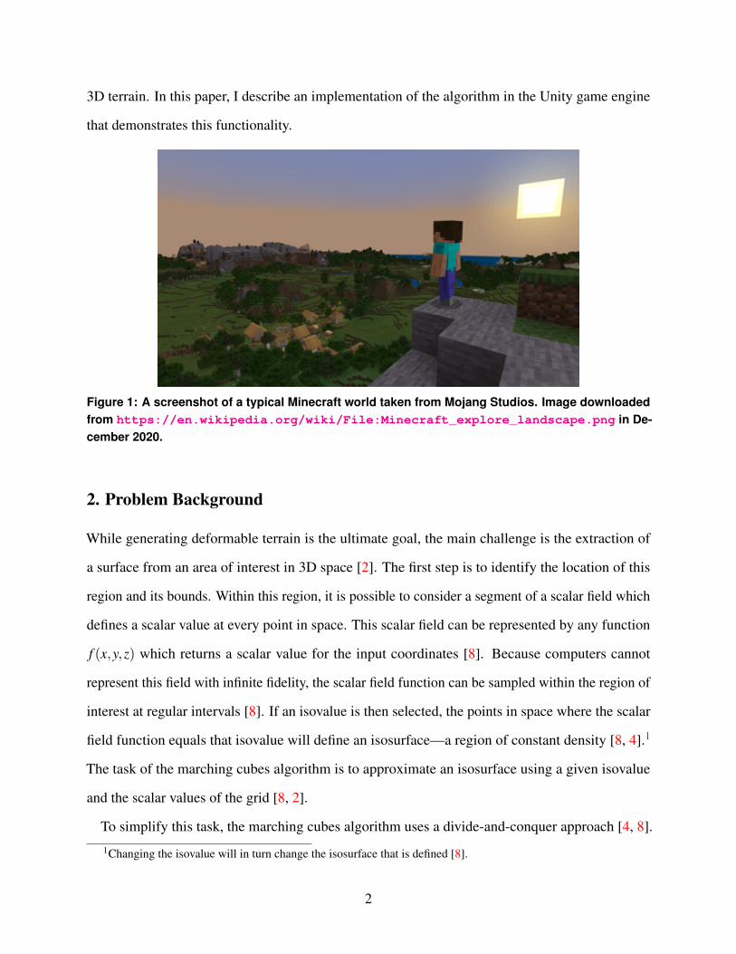
3D terrain. In this paper, I describe an implementation of the algorithm in the Unity game engine
that demonstrates this functionality.
Figure 1: A screenshot of a typical Minecraft world taken from Mojang Studios. Image downloadedfrom https://en.wikipedia.org/wiki/File:Minecraft_explore_landscape.png in De-cember 2020.
2. Problem Background
While generating deformable terrain is the ultimate goal, the main challenge is the extraction of
a surface from an area of interest in 3D space [2]. The first step is to identify the location of this
region and its bounds. Within this region, it is possible to consider a segment of a scalar field which
defines a scalar value at every point in space. This scalar field can be represented by any function
f (x,y,z) which returns a scalar value for the input coordinates [8]. Because computers cannot
represent this field with infinite fidelity, the scalar field function can be sampled within the region of
interest at regular intervals [8]. If an isovalue is then selected, the points in space where the scalar
field function equals that isovalue will define an isosurface—a region of constant density [8, 4].1
The task of the marching cubes algorithm is to approximate an isosurface using a given isovalue
and the scalar values of the grid [8, 2].
To simplify this task, the marching cubes algorithm uses a divide-and-conquer approach [4, 8].
1Changing the isovalue will in turn change the isosurface that is defined [8].
2

Because the scalar field is considered on a structured, uniform grid, each set of eight points makes
up the vertices of a logical cube [4]. The key optimization made by the algorithm is the use of
lookup tables. Each vertex is associated with a position in an 8-bit index, with that position being
set depending on whether the given vertex is above or below the isosurface [4, 8, 2]. In other words,
the index describes the configuration of the current cube. This index is mapped to a particular
triangulation using a case-table [4, 8, 2]. The next cube is then “marched,” creating a full mesh
when the entire grid has been considered. In this way, the geometry of a cube in the grid is not
actually affected by its neighbors [8].
Determining the triangulation of each case, however, presents its own difficulties. Because
there are eight vertices per cube, and two states that each vertex can take, there are a total of
28 = 256 possible ways for an isosurface to intersect the cube—and therefore an equal number of
possible triangulations [4, 8]. While this is a large amount when considered at face-value, the use of
complementary and rotational symmetries means that only 15 different configurations need to be
calculated manually [4, 8]. Figure 2 illustrates each of these configurations.
Figure 2: The original 15 published cases, as represented by Wikipedia user Jmtrivial in 2006. Im-age downloaded from https://commons.wikimedia.org/wiki/File:MarchingCubes.svg
in December 2020.
3

3. Related Work
Originally published by Lorensen and Cline during the proceedings of the 1987 SIGGRAPH
conference [4], marching cubes is likely the most well known algorithm for extracting a polygonal
mesh from a scalar field. It is well documented, and a variety of implementations have been
described across different platforms [4, 2, 1]. The original motivation for the marching cubes
algorithm was to improve the visualization of medical data, something that existing techniques
struggled to accomplish with high levels of detail [4]. As Figure 3 illustrates, the algorithm is
capable of handling discrete data produced from MRI scans, CT scans, and other technologies [4].
Figure 3: A polygonal mesh extracted from 150 MRI slices using marching cubes, created by Wikipediauser Dake in 2005. Image downloaded from https://commons.wikimedia.org/wiki/File:
Marchingcubes-head.png in December 2020.
The authors also describe several enhancements to the algorithm. Of particular relevance is the
use of linear interpolation to place vertices on intersected edges [4]. While it would be possible to
simply place vertices at the midpoint of intersected edges each time, this results in a blockier mesh.
Although linear interpolation assumes that the values in the scalar field always change linearly, it
still produces a smoother mesh that better approximates the original isosurface. As Sockalingam [8]
4

observes, the interpolation does not interfere with how these vertices are connected to each other;
connections depend only on the state of each vertex with regards to being above or below the
isosurface.
While Lorensen and Cline focused on the visualization of existing datasets, my project seeks to
produce the scalar field from a function as described by Sockalingam and Bourke [8, 2]. This scalar
field function will in turn generate a surface that resembles real terrain. Furthermore, although the
original paper discusses solid modeling as a functional enhancement to the marching cubes algo-
rithm [4], attention remains for the most part on the static representation of data. Sockalingam [8]
notes that the speed of marching cubes makes it suitable for real-time environments, even if the
mesh is regenerated every frame. My project aims to leverage this quality to make the extracted
mesh truly interactive.
4. Approach
The creation of 3D terrain that can be deformed in real time requires two key components. The first
is the representation of the terrain itself. Given the discussion of scalar field functions and their
role in isosurface extraction, I intended to find an appropriate function to use for sampling. While
the extraction process itself does not change based on the sampled values,2 the focus on terrain
specifically led me towards functions that could approximate natural landscapes.
The other component—and arguably the one most important for interactivity—is the treatment of
the grid points that sample the scalar field. This meant converting grid points into dynamic entities
that could respond to input. If the user is then given a way to change the scalar values within a
region of the grid, the extracted surface could change interactively. By regenerating the mesh each
time a value change is detected within the grid, any deformation would appear to occur in real time.
2Indeed, as described in the problem background any function at all could be used. The only requirement for themarching cubes algorithm is that a scalar value is defined for every point in the grid.
5

5. Implementation
In the following subsections, I will explain the implementation process and describe each component
of the final application.
5.1. Tool Selection
With visualization and user interaction at the core of my project, the choice of development
environment was critical. Game engines are a natural fit, because they provide a framework that
is well-suited to handling complex graphics and user input. In particular, the Unity game engine
was selected for its ease-of-use during development. Unity is arguably one of the most popular
game engines that is available for free use, and its rich documentation is supplemented by a large
and active community online. The use of C# for scripting meant that I could easily transfer my
prior experience with Java and other—syntactically-similar—programming languages. Finally, and
perhaps most importantly, Unity is multi-platform. This meant that I could use the same assets to
build executables for Windows, Mac, and Linux.
The actual code for the project was written using Visual Studio, a complete integrated development
environment by Microsoft that is bundled with Unity. Git was used to version-control all project
assets, while GitHub was used to synchronize the repository across multiple devices.
5.2. Scalar Field Representation
The selection of the scalar field function ultimately determines the surfaces that can be extracted.
To this end, I wanted to find a noise function that could reliably produce natural-looking terrain.
Unity includes its own implementation of Perlin noise with the function Mathf.PerlinNoise [10],
which takes a 2D coordinate and returns a value between 0.0 and 1.0. The strength of Perlin noise is
that it is pseudo-random; the values at each coordinate change in a gradual way [10]. This results
in a gradient that is far more natural than pure noise, making the function appropriate for terrain
generation.
To actually use Perlin noise, it was also necessary to consider the representation of the grid that
6

would sample the scalar field. In the final implementation, a GridPoint class was constructed
that tracks the position and value of a single point in the grid. The grid itself is simply a 3D array
of these GridPoints. When the grid is first initialized, or alternately when the user presses the
R key, the scalar field is sampled for each point in the grid. As Listing 1 illustrates, this is
accomplished by iterating over the entire grid and calling Mathf.PerlinNoise each time.
Listing 1: Sampling a scalar field created with Perlin noise.
grid[x, y, z].Value = Mathf.PerlinNoise(x, z) * y;
Because Unity’s implementation of Perlin noise is limited to a 2D plane [10], it was necessary
to multiply the value returned by Mathf.PerlinNoise by the y-component of the current point.
Additionally, in order to account for the scale of the grid as selected in the Unity editor,3 each
component is divided by the size of the grid in that direction and then multiplied by the selected
zoom level. These new values are what is actually used in the final sampling code. Listing 2
illustrates this transformation.
Listing 2: Accounting for grid scale during sampling.
1 float nx = Zoom * (x / GridSize.x);
2 float ny = Zoom * (y / GridSize.y);
3 float nz = Zoom * (z / GridSize.z);
In the interactive demo, this process gives the appearance of a flat plane that has been displaced
on the y-axis in order to create hills. Of note, Perlin noise will return the same value if given
identical coordinates. To produce different terrain each time, a pseudorandom seed is generated
before sampling. This seed is added to each component passed to Mathf.PerlinNoise, effectively
sampling from a different region of the gradient each time. A more sophisticated use of Perlin
noise might layer additional layers of noise at different frequencies, creating finer details, or extend
Unity’s implementation to three dimensions to create more complex geometry.3The final application uses a zoom level of 3.0.
7

To decrease visual ambiguity, the bounds of the grid are visualized during program execution.
Unity provides the LineRenderer class [9], which takes an array of at least two points and draws
straight lines between each one. To draw the grid boundaries, a LineRenderer instance is created
on startup. Its points are then set in sequence to match the corners of the grid volume.
5.3. Case-Table Selection
As explained in the problem background, the marching cubes algorithm is dependent on lookup
tables to handle each possible configuration. In this sense, these tables are arguably just as important
as the algorithm itself. While Lorensen and Cline reduce the number of cases that need to be
computed manually to 15 [4, 8], this still presented a significant barrier to actually using marching
cubes in my project. To ensure the correctness of my own implementation, I decided to use the
triangulation tables created by Bloyd [1] and later reused by Bourke [2].
As explained by Bourke [2], the first table (called edgeTable in my implementation) is a 256-
element array of numbers. The table takes an index representing the current cube configuration and
maps it to a single 12-bit number represented in hexadecimal. This number in turn describes which
edges of the cube are intersected by the isosurface, with each bit corresponding to the state of a
single edge [2].
The second table (called triangleTable in my implementation), is a 2D array. Like the previous
table, the index representing the current configuration is used as a pointer into the array [2]. However,
here the index maps to a 16-element integer array that describes the specific triangulation of the
intersected points [1, 2]. Each triangle is represented by three consecutive integers, with each integer
corresponding to the intersected point of a specific edge [1]. Because some configurations contain
less triangles than others, the end of a sequence is marked by the value -1 when necessary [1].
5.4. Algorithm Implementation
My implementation of the marching cubes algorithm is contained within a single script, called
MarchingCubes.cs, but it required additional logic before it could be used in my project. To
accomplish this, another script called Generate.cs was created. Apart from handling some user
8

input, the code in this file is what actually drives the bulk of the final application. This includes
initializing the grid on startup, sampling the scalar field function, running the marching cubes
algorithm, and building the final mesh.
Unity allows for the programmatic creation and modification of meshes through the Mesh
class [11]. At a minimum, mesh creation requires a set of vertices and a set of triangles that will
ultimately form the basic geometry [11]. To represent both vectors and positions in 3D space, Unity
uses the Vector3 structure [13]. For the Mesh class, vertices are stored as an array of Vector3
instances [11]. Another array contains a sequence of integers that describe the triangles used for
the mesh, with each integer serving as an index into the vertex array [11]. In Generate.cs, a new
Mesh is obtained every time the isosurface is extracted from the scalar field. As the marching cubes
algorithm iterates over every cell in the grid, it determines the necessary vertices and triangles for
the current configuration. These are then added to a master vertex and triangle list, which then sets
the geometry of the final mesh.
This operation, however, also required thinking about the communication between my marching
cubes implementation and Generate.cs. Because the marching cubes algorithm works on one
logical cube at a time, it was necessary to package the required information before performing any
necessary operations. The MarchingCubes.cs script defines two additional classes that make this
possible. The first is a simple Triangle class, which consists of three Vector3 instances defining
the vertices of a single triangle in 3D space. The second class, GridCell, is more involved and
supplements the GridPoint class described earlier. The GridCell class maintains an array of
eight GridPoints, an array of Triangles, and an array of Vector3 instances that are used to
form each triangle for the current configuration.
A single instance of the GridCell class is used by Generate.cs. When the isosurface is
extracted or re-extracted by the application, every point of the grid is iterated over. Using the
coordinates of each point, the seven other vertices that make up a single cube can also be found.
With this information, the vertices of the GridCell instance can be set to the corresponding
GridPoints. The marching cubes implementation in MarchingCubes.cs provides a single
9

access point, the function Triangulate, that performs all necessary computation. Once the corners
of the cube are defined, a reference to the associated GridCell and the selected isolevel are passed
to the function for triangulation.
The marching cubes algorithm, as discussed in the problem background, first requires an index to
be computed for use with the lookup tables. Lorensen and Cline [4] describe an 8-bit index, with
each bit corresponding to the state of a particular vertex. However, they do not specify the exact
format. In my implementation, a single integer is used to represent the index. While the int type
in C# defaults to a signed 32-bit integer [5], the extra information can simply be ignored when
indexing into each table. While other index representations are possible,4 their usage would be
identical.
Listing 3 illustrates the logic used to find the index. Each GridPoint is checked to determine
if its value is less than the given isovalue, which signifies that it is inside the surface. If it is,
the corresponding bit is set in the index before considering the next GridPoint. While it would
be possible to unroll the loop and perform this check manually for each vertex, using a for-loop
improved the conciseness of the final code. Of note is the use of two bitwise operations in the
expression index |= 1 << i to actually set the correct bit. The value 1 is shifted left a number
of positions equal to i, which accommodates the current value of the loop control variable. When
the exclusive-or of this operand and index is taken, this effectively sets the bit at the appropriate
position.
4It is worth noting that C# provides the BitArray [6] class specifically for managing bit values, and it would alsobe possible to use a bool array. More work is needed to determine if either approach provides any meaningful space orperformance benefits.
10

Listing 3: Calculating the index for the current configuration.
1 int index = 0;
2 for (int i = 0; i < 8; i++)
3 {
4 if (cell.p[i].Value < isolevel)
5 {
6 index |= 1 << i;
7 }
8 }
Once the index has been calculated, it is necessary to find where the isosurface meets each
intersected edge in the cube. This information will later be used to construct the triangles needed for
the current configuration. In order to determine which edges are intersected, the first of Bloyd’s [1]
lookup tables is used. Once an intersected edge has been identified, linear interpolation is used to
estimate the actual point of intersection along the edge. Finally, the intersection point is added to
the GridCell at the corresponding position. Listing 4 illustrates this operation.
Listing 4: Calculating the intersection point for each edge in the cube.
1 if (edgeTable[index] == 0) return;
2 for (int i = 0; i < 12; i++)
3 {
4 if ((edgeTable[index] & (1 << i)) != 0)
5 {
6 cell.edgepoints[i] =
7 Interpolate(cell.p[vertexTable[i, 0]],
8 cell.p[vertexTable[i, 1]],
9 isolevel);
10 }
11 }
Because this table provides the intersection data in the form of a 12-bit number, a bitwise
operation similar to that used in the index calculation is required. Additionally, a check is made
before the for-loop is entered. This simply returns if the GridCell is not intersected at any edge,
11
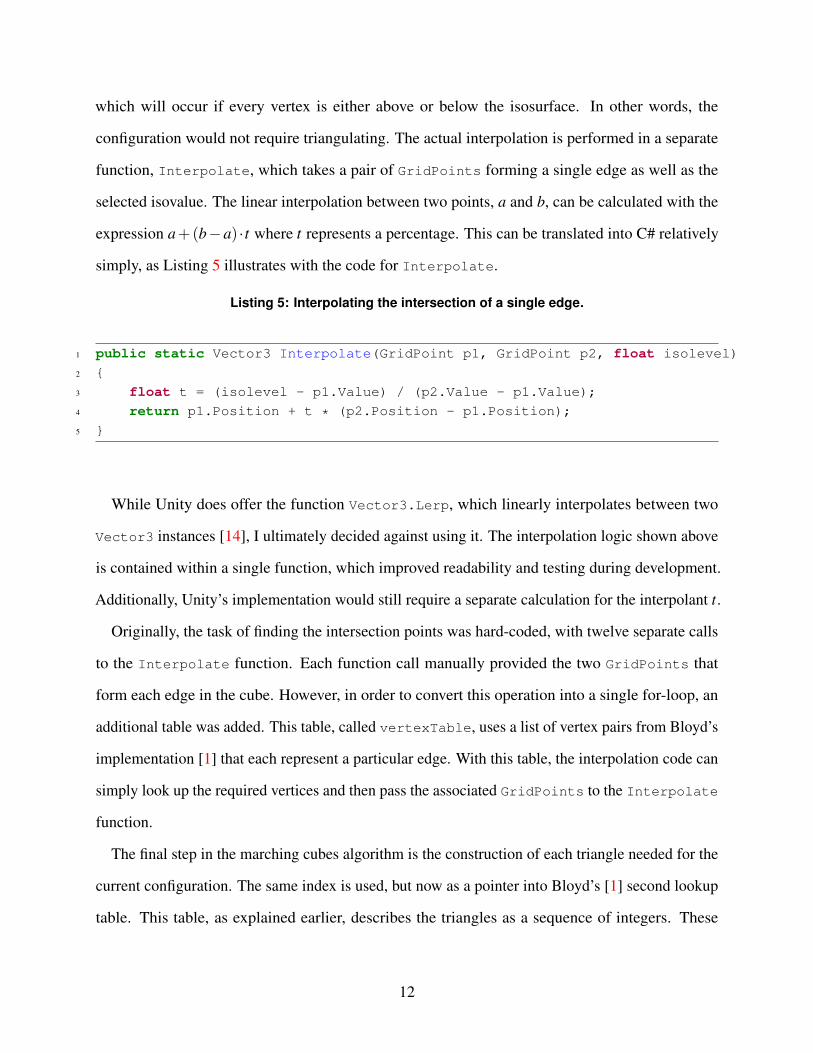
which will occur if every vertex is either above or below the isosurface. In other words, the
configuration would not require triangulating. The actual interpolation is performed in a separate
function, Interpolate, which takes a pair of GridPoints forming a single edge as well as the
selected isovalue. The linear interpolation between two points, a and b, can be calculated with the
expression a+(b−a) · t where t represents a percentage. This can be translated into C# relatively
simply, as Listing 5 illustrates with the code for Interpolate.
Listing 5: Interpolating the intersection of a single edge.
1 public static Vector3 Interpolate(GridPoint p1, GridPoint p2, float isolevel)
2 {
3 float t = (isolevel - p1.Value) / (p2.Value - p1.Value);
4 return p1.Position + t * (p2.Position - p1.Position);
5 }
While Unity does offer the function Vector3.Lerp, which linearly interpolates between two
Vector3 instances [14], I ultimately decided against using it. The interpolation logic shown above
is contained within a single function, which improved readability and testing during development.
Additionally, Unity’s implementation would still require a separate calculation for the interpolant t.
Originally, the task of finding the intersection points was hard-coded, with twelve separate calls
to the Interpolate function. Each function call manually provided the two GridPoints that
form each edge in the cube. However, in order to convert this operation into a single for-loop, an
additional table was added. This table, called vertexTable, uses a list of vertex pairs from Bloyd’s
implementation [1] that each represent a particular edge. With this table, the interpolation code can
simply look up the required vertices and then pass the associated GridPoints to the Interpolate
function.
The final step in the marching cubes algorithm is the construction of each triangle needed for the
current configuration. The same index is used, but now as a pointer into Bloyd’s [1] second lookup
table. This table, as explained earlier, describes the triangles as a sequence of integers. These
12
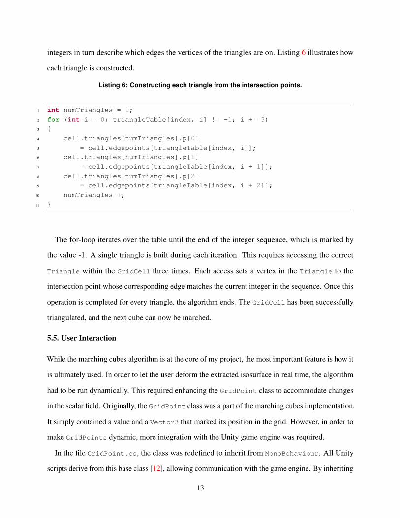
integers in turn describe which edges the vertices of the triangles are on. Listing 6 illustrates how
each triangle is constructed.
Listing 6: Constructing each triangle from the intersection points.
1 int numTriangles = 0;
2 for (int i = 0; triangleTable[index, i] != -1; i += 3)
3 {
4 cell.triangles[numTriangles].p[0]
5 = cell.edgepoints[triangleTable[index, i]];
6 cell.triangles[numTriangles].p[1]
7 = cell.edgepoints[triangleTable[index, i + 1]];
8 cell.triangles[numTriangles].p[2]
9 = cell.edgepoints[triangleTable[index, i + 2]];
10 numTriangles++;
11 }
The for-loop iterates over the table until the end of the integer sequence, which is marked by
the value -1. A single triangle is built during each iteration. This requires accessing the correct
Triangle within the GridCell three times. Each access sets a vertex in the Triangle to the
intersection point whose corresponding edge matches the current integer in the sequence. Once this
operation is completed for every triangle, the algorithm ends. The GridCell has been successfully
triangulated, and the next cube can now be marched.
5.5. User Interaction
While the marching cubes algorithm is at the core of my project, the most important feature is how it
is ultimately used. In order to let the user deform the extracted isosurface in real time, the algorithm
had to be run dynamically. This required enhancing the GridPoint class to accommodate changes
in the scalar field. Originally, the GridPoint class was a part of the marching cubes implementation.
It simply contained a value and a Vector3 that marked its position in the grid. However, in order to
make GridPoints dynamic, more integration with the Unity game engine was required.
In the file GridPoint.cs, the class was redefined to inherit from MonoBehaviour. All Unity
scripts derive from this base class [12], allowing communication with the game engine. By inheriting
13

from MonoBehaviour, the GridPoint class could be attached as a component and react to the
main game loop. When Generate.cs initializes the grid, it creates an empty game object at every
point and attaches both a GridPoint instance and a collider.
If any of the game objects detects a collision, the associated GridPoint checks if the user wants
to add to its scalar value or subtract from it. Regardless of the direction, the change is made
with respect to the time difference from the last frame. This ensures that any change in value is
independent of the frame rate. In addition, the value of the GridPoint is always clamped between
0.0 and 1.0. Restricting the scalar value means that a change to it can be reversed in a short amount
of time, preventing the deformation process from feeling too slow.
If the value of a GridPoint is changed, the isosurface needs to be re-extracted from the scalar
field. This is handled through a C# event, which is declared in the GridPoint class and delegated
to Generate.cs. Any value change will trigger the event, which sets a flag in Generate.cs to
regenerate the mesh. This operation will be carried out in the next frame if the flag is set, which
helps prevent repeated build calls from stacking.
While this logic allows for real-time deformation, the user still needs a way to actually interact
with the terrain. To solve this problem, I introduced the concept of a “brush.” This brush consisted
of a sphere primitive, a translucent material, and a collider slightly larger than the actual object.
By locking the brush’s position to a fixed distance from the main camera, it would always remain
in view as the user moved and looked around the scene. The left and right mouse buttons, when
pressed, set flags that add and subtract values in the region defined by the collider. When the user is
not pressing either button, the brush’s collider is disabled to prevent interaction with the grid. In
effect, the brush can be used to seamlessly edit the terrain.
To enable the user to look and move around, I adapted a script posted by user IJM [3] on the
Unity online forum. The script was modified to support using the brush, and the movement controls
were also changed to match those seen in Minecraft. As previously mentioned, Generate.cs also
handles some user input. When the user presses the R key to create new terrain, the texture used
for the mesh is picked at random from several different options. When the C key is pressed,
14
every GridPoint is given the value 1.0. This results in no visible mesh, giving the user the entire
grid to draw in.
5.6. Application Deployment
To make my project available outside of the Unity editor, I used the engine’s provided tools to
package and export the final application. Versions for both Windows and Mac have been tested, but
a Linux build should also be possible. While I intended to host a WebGL build as well, it was not
functional outside of basic movement. Further testing is required to determine the source of the
problem.
6. Evaluation
Because the goal of my project was to use marching cubes interactively, the performance of the
algorithm was critical. This concerns the initial triangulation on startup, but also the behavior of the
algorithm when the user continuously edits the generated terrain. The primary evaluation was the
time required to triangulate the mesh once. More specifically, a number of grid sizes were tested to
find how long the algorithm took to triangulate increasingly larger regions of space. C# provides a
Stopwatch class that can be used to accurately measure and record time [7].
In Generate.cs, a StopWatch instance is created every time the mesh is regenerated. After the
isosurface is extracted, the elapsed time in milliseconds is printed to the Unity Console. Six grid
dimensions were tested, ranging from a 1×1×1 grid to one that was 50×50×50. All tests were
run on a desktop computer with an NVIDIA GeForce 1080 Ti graphics card and an Intel Core i5
processor clocked at 3.5GHz. As Table 1 illustrates, at no point was more than 100 milliseconds
required to triangulate the scalar field.
It is also worth mentioning the overall frame rate. In general, the application exceeded 2000
frames per second at grid sizes below 30×30×30. Drops to 600 FPS, however, occurred when the
mesh was being continuously regenerated by the brush. At larger dimensions, the average frame
rate was lowered to double-digits. An interesting observation is that the marching cubes algorithm
does not appear to be the main performance bottleneck. Indeed, the larger grid sizes show that it is
15

Grid Size Time (ms)1×1×1 < 110×10×10 120×20×20 630×30×30 1940×40×40 4450×50×50 83
Table 1: Time to triangulate mesh once.
actually rendering the triangulated mesh that slows the application the most. In my implementation,
adjacent cubes are not able to share vertices. This ultimately contributes to the complexity of the
mesh growing faster than is necessary. The Unity Editor itself also adds overhead, a fact that likely
affected the reported numbers during testing.
7. Conclusions and Future Work
The beauty of the marching cubes algorithm is in its simplicity. Because each triangulation is
precomputed, most of the work can be accomplished by indexing into the correct lookup table.
My project shows that marching cubes is not only viable for real-time applications, but also that it
improves the quality of generated terrain. The algorithm remained performant during periods of
high utilization, and produced results that were more convincing than a voxel-based approach. I
originally wanted to create deformable 3D terrain, and I believe my project has more than succeeded
in that goal.
With this success in mind, there is still a wealth of possible work that can and should be explored.
My project only touched the surface of this algorithm’s potential, and even the focus on terrain
specifically could be expanded much further. For one, my use of Perlin noise was relatively limited.
More sophisticated approaches to noise generation exist, and they have the potential to create more
interesting surfaces with higher levels of detail.
The algorithm itself is also open to improvement. Sockalingam [8] notes that the 15 originally
published cases allow for holes between adjacent grid cells. The behavior of the scalar field
is also not taken into account during triangulation, which can lead to ambiguities in the final
16

mesh [8]. Expanded implementations of the marching cubes algorithm have attempted to solve these
problems [8], and it would be interesting to evaluate them in the context of real-time applications.
Finally, my marching cubes implementation does not leverage the GPU. Because neighboring
cubes do not affect each other’s geometry, the algorithm is well-suited to parallel computation [8].
In Unity, it is possible to write compute shaders that will run on the available graphics hardware.
The greatest optimization potential is likely here, and a future implementation of marching cubes
using compute shaders could drastically improve performance.
Acknowledgements
I graciously thank my adviser, Professor Szymon Rusinkiewicz, for enabling me to undertake this
project. It was a privilege to explore an interesting algorithm in such detail, and I am a better
computer scientist because of it. I also thank all my friends and family. Their tireless support during
the semester made this project possible.
Honor Code
I pledge my honor that this paper represents my own work in accordance with University regulations
/s/ William Svoboda
17

References[1] C. G. Bloyd, “Marching cubes example program,” n.d., source code. Available: http://paulbourke.net/geometry/
polygonise/marchingsource.cpp[2] P. Bourke, “Polygonising a scalar field,” May 1994, webpage. Available: http://paulbourke.net/geometry/
polygonise/[3] IJM, “Mouselook.cs,” October 2010, source code. Available: http://answers.unity.com/answers/29758/view.html[4] W. E. Lorensen and H. E. Cline, “Marching cubes: A high resolution 3d surface construction algorithm,”
in Proceedings of the 14th Annual Conference on Computer Graphics and Interactive Techniques, ser.SIGGRAPH ’87. New York, NY, USA: Association for Computing Machinery, 1987, p. 163–169. Available:https://doi.org/10.1145/37401.37422
[5] Integral Numeric Types, Microsoft Corporation, October 2019. Available: https://docs.microsoft.com/en-us/dotnet/csharp/language-reference/builtin-types/integral-numeric-types
[6] BitArray Class, Microsoft Corporation, n.d., .Net 5.0. Available: https://docs.microsoft.com/en-us/dotnet/api/system.collections.bitarray?view=net-5.0
[7] Stopwatch Class, Microsoft Corporation, n.d., .Net 5.0. Available: https://docs.microsoft.com/en-us/dotnet/api/system.diagnostics.stopwatch?view=net-5.0
[8] K. Sockalingam, “Isosurface mesh extraction from scalar fields: Marching cubes vs dual contouring,” October2016, unpublished. Available: http://kieranvs.com/files/isosurface.pdf
[9] Line Renderer, Unity Technologies, December 2020, version 2019.4. Available: https://docs.unity3d.com/2019.4/Documentation/Manual/class-LineRenderer.html
[10] Mathf.PerlinNoise, Unity Technologies, December 2020, version 2019.4. Available: https://docs.unity3d.com/2019.4/Documentation/ScriptReference/Mathf.PerlinNoise.html
[11] Mesh, Unity Technologies, December 2020, version 2019.4. Available: https://docs.unity3d.com/2019.4/Documentation/ScriptReference/Mesh.html
[12] MonoBehaviour, Unity Technologies, December 2020, version 2019.4. Available: https://docs.unity3d.com/2019.4/Documentation/ScriptReference/MonoBehaviour.html
[13] Vector3, Unity Technologies, December 2020, version 2019.4. Available: https://docs.unity3d.com/2019.4/Documentation/ScriptReference/Vector3.html
[14] Vector3.Lerp, Unity Technologies, December 2020, version 2019.4. Available: https://docs.unity3d.com/2019.4/Documentation/ScriptReference/Vector3.Lerp.html
A. Appendix
All project code is hosted on GitHub at https://github.com/thisstillwill/IW-Fall-2020
along with links to builds of the final application.
18