IMPROVING START-UP AND STEADY-STATE

BEHAVIOR OF TCP IN HIGH BANDWIDTH-DELAY

PRODUCT NETWORKS

by

DAN LIU

Submitted in partial fulfillment of the requirements

For the degree of Master of Science

Thesis Adviser: Dr. Shudong Jin

Department of Electrical Engineering and Computer Science

CASE WESTERN RESERVE UNIVERSITY

August, 2007

Improving Start-up and Steady-state Behavior of TCP in

High Bandwidth-Delay Product Networks

Approved by

Thesis Committee:

Dr. Shudong Jin

Dr. Vincenzo Liberatore

Dr. Michael Rabinovich

Mark Allman (Ad hoc Committee)

III

To Grandpa 

Zhongyi Xiao 

 

 Mom and Dad 

Yuyou Xiao and Yanming Liu 

Contents

Contents ........................................................................................................................... IV

List of Tables ................................................................................................................... VI

List of Figures ................................................................................................................ VII

Acknowledgement ........................................................................................................... IX

Abstract ............................................................................................................................. X

Chapter 1 Introduction.................................................................................................. 1

1.1 Motivation ...................................................................................................... 1

1.2 Approaches and Results ................................................................................. 3

1.3 Thesis Organization ....................................................................................... 4

Chapter 2 Background and Related Work .................................................................. 5

2.1 TCP Congestion Control Overview ............................................................... 5

2.1.1 Slow Start ................................................................................................. 6

2.1.2 Congestion Avoidance ............................................................................. 7

2.2 TCP Congestion Control Modifications ........................................................ 8

2.2.1 Previous Modifications to Slow Start ...................................................... 8

2.2.2 Previous Modifications to Congestion Avoidance ................................. 10

Chapter 3 Improving TCP Start-up Behavior Using Jump Start ........................... 12

3.1 Problem Description .................................................................................... 12

3.2 Jump Start .................................................................................................... 13

3.3 Simulations and Results ............................................................................... 15

3.3.1 Single FTP Flows ................................................................................... 18

3.3.2 Competing FTP Flows ........................................................................... 22

3.3.3 Mixed FTP Flows .................................................................................. 24

3.3.4 Web Traffic ............................................................................................ 26

IV

3.3.5 Active Queue Management .................................................................... 29

3.4 Coping Methods ........................................................................................... 32

3.5 Summary ...................................................................................................... 33

Chapter 4 Improving TCP Steady-state Behavior Using EXP-TCP ...................... 34

4.1 TCP Variants for High BDP Networks ........................................................ 34

4.2 EXP-TCP ..................................................................................................... 39

4.2.1 EIMD Algorithm .................................................................................... 39

4.2.2 Algorithm Analysis ................................................................................ 40

4.3 Simulations and Results ............................................................................... 42

4.3.1 Impact of Bottleneck Capacity ............................................................... 43

4.3.2 Impact of Number of Flows ................................................................... 46

4.3.3 Impact of Web Traffic ............................................................................ 46

4.3.4 Convergence to Fairness ........................................................................ 49

4.3.5 Response to Sudden Changes ................................................................ 53

4.4 Summary ...................................................................................................... 57

Chapter 5 Conclusions and Future Work ................................................................. 58

5.1 Summary ...................................................................................................... 58

5.2 Future Research............................................................................................ 59

Bibliography .................................................................................................................... 60

V

VI

List of Tables

Table 3. 1 Network configuration ...................................................................................16

Table 3. 2 Scenario design and specified parameter settings ..........................................17

Table 3. 3 Parameters of the Web traffic simulation .......................................................27

List of Figures

Figure 2. 1 An illustration of evaluation of TCP congestion window size ......................6

Figure 3. 1 Simulation topology: Dumb-bell ................................................................15

Figure 3. 2 Percent improvement and drop rate increase of Jump Start compared with Slow Start across a variety of bottleneck capacities ...................................19

Figure 3. 3 Percent improvement for Jump Start when compared with Slow Start as a function of one-way bottleneck delay .........................................................21

Figure 3. 4 Connection duration and aggregate drop rate as a function of start interval: Jump Start vs. Slow Start ............................................................................23

Figure 3. 5 Median connection duration and median drop rate as a function of the fraction of Jump Start flows: Jump Start vs. Slow Start .............................25

Figure 3. 6 Distributions of connection duration and aggregate drop rates: Jump Start vs. Slow Start ..............................................................................................28

Figure 3. 7 Connection duration as a function of transfer size: Jump Start vs. Slow Start, DropTail vs. RED ..............................................................................30

Figure 3. 8 Connection duration and aggregate drop rate as a function of start interval: Jump Start vs. Slow Start, DropTail vs. RED .............................................31

Figure 4. 1 An illustration of the congestion window size evolution of EXP-TCP ......41

Figure 4. 2 Performance of control algorithms when the bottleneck capacity ranges from 2.5Mbps to 5.12Gbps .........................................................................45

Figure 4. 3 Performance of congestion control algorithms when the number of long-lived flows ranges from 2 to 512 ........................................................47

Figure 4. 4 Performance of congestion control algorithms when the background Web-like flows consumes between 2% and 51.2% of the bottleneck capacity .......................................................................................................48

Figure 4. 5 Convergence to fairness of competing flows when DropTail is used: TCP vs. HSTCP vs. STCP vs. EXP-TCP ............................................................50

Figure 4. 6 Convergence to fairness of competing flows when RED is used: TCP vs. HSTCP vs. STCP vs. EXP-TCP ..................................................................50

Figure 4. 7 Fairness Index: TCP vs. HSTCP vs. STCP vs. EXP-TCP ..........................52

Figure 4. 8 Changes of the average throughput of competing flows in response to the

VII

VIII

sudden changes of traffic demands: TCP vs. HSTCP vs. STCP vs. EXP-TCP ....................................................................................................54

Figure 4. 9 Changes of bottleneck utilization in response to the sudden changes of traffic demands: TCP vs. HSTCP vs. STCP vs. EXP-TCP .........................55

Figure 4. 10 Changes of bottleneck queue occupation in response to the sudden changes of traffic demands: TCP vs. HSTCP vs. STCP vs. EXP-TCP .....................56

Acknowledgement

I would like to express my most sincere gratitude to Dr. Shudong Jin, my advisor, for his

guidance, inspiration and support throughout my M.S. program. I am indebted to him for

the opportunity that he gave me to achieve my personal endeavors. He inspired me to go

beyond the limits of what I thought was possible. He was deeply engaged with me from

the formative stage, through the refining of this work to the final writing. His great

patience and deep understanding make me feel forever grateful toward him.

I would like also thank Mark Allman and Dr. Limin Wang for their instructions and

suggestions during the writing of this thesis. Their patient advice always encouraged me

to work hard. Without their support, this work would never have been completed.

I feel very thankful to my advisory committee members, Dr. Vincenzo Liberatore

and Dr. Michael Rabinovich, for their effort to read this thesis and give me valuable

comments and suggestions, and eventually evaluate my work.

Finally, great thanks go to my beloved father Yanming Liu and mother Yuyou Xiao

for their endless support and love. Special thanks go to my grandfather Zhongyi Xiao for

his lifetime love. Last but not least, are thanks to all my dear friends in Case Western

Reserve University for their friendship and help during my studies.

IX

Improving Start-up and Steady-state Behavior of TCP in High

Bandwidth-Delay Product Networks

Abstract

by

DAN LIU

It has been long known that the standard Transmission Control Protocol (TCP) yields

limited performance in high bandwidth-delay product (BDP) networks due to its

conservative Slow Start and Congestion Avoidance algorithms. In this work, we focus on

TCP modifications to improve both TCP’s start-up and steady-state behavior.

First, we propose Jump Start, a new technique which has the potential to speedup the

start-up of TCP by ignoring the Slow Start. It allows a higher initial sending rate but

keeps the remaining of TCP unchanged. Simulations show both positive and negative

implications of Jump Start on TCP performance. Second, we introduce EXP-TCP, a new

TCP variant which replaces the additive-increase rule of the Congestion Avoidance with

an exponential-increase algorithm. It decouples TCP efficiency control and fairness

control to achieve both high performance and good fairness. Simulations indicate that

EXP-TCP provides higher performance and better fairness than TCP in high BDP

networks.

X

Chapter 1

Introduction

1.1 Motivation

The Transmission Control Protocol (TCP) [J88] is the most popular transport layer

protocol in the Internet for reliable data transmission. It has had a significant impact on

the performance and behavior of the Internet [TMW97]. However, it has been long

known for its unsatisfactory performance in high bandwidth-delay product (BDP)

networks. Such performance limitation comes from TCP’s conservative congestion

control algorithms which are unable to cope with the features of high BDP networks, i.e.,

the large per-flow throughput or long propagation delay that requires high outstanding

traffic in the pipe during transmission [CO02]. Maintaining a high volume of outstanding

traffic in turn requires that the TCP source set a large congestion window size (cwnd).

The two main algorithms of standard TCP, i.e., Slow Start and Congestion

Avoidance [J88], both have been hindrances for TCP’s high performance in high BDP

networks. First, Slow Start, the initial phase of a TCP connection before reaching a

reasonably high congestion window size, could be time-consuming in high BDP

environment. Although the sender’s congestion window size is increased exponentially

during Slow Start, the initial sending rate, as low as one packet per round-trip time (RTT),

is too conservative for the sender to make full use of the available large capacity. Second,

the Additive Increase Multiplicative Decrease algorithm (AIMD) of Congestion

Avoidance also holds back the performance of TCP in high BDP networks. For example,

1

when a large amount of bandwidth becomes suddenly available after a period of

congestion, it may take TCP too long to linearly recover from its huge back-off to full

utilization.

To solve all these problems, many TCP modifications have been extensively studied

(e.g., [AHO98], [K03], [LPW01], [XSSK05]). For Slow Start, a number of alternatives

have been proposed (e.g., [AHO98], [AP99], [BRS99], [FAJS06], [PRAKS02]). They

enable the sender to reach an appropriate congestion window size faster, but the

improvement is still unsatisfactory because they either require extra assistance from the

network or turn to be hard to achieve both efficiency and fairness at the same time. On

the other hand, two main categories of modifications have been suggested for Congestion

Avoidance. One is based on end-to-end congestion controls (e.g., [F03], [K03],

[XHR04]); the other one uses router-assisted mechanisms (e.g., [K03a], [LAW05],

[XSSK05]). They both emphasize more aggressive increasing behavior at the sender

during Congestion Avoidance phase, but unfortunately they either worsen the unfairness

problem, or introduce additional complexity to other network components, such as the

routers. In Chapter 2, a more detailed introduction will be provided to all these

modifications as well as their pros and cons.

In this thesis, our goal is to explore new modifications to TCP which can achieve

both high efficiency and good fairness in high BDP networks, only from an end-to-end

perspective.

2

1.2 Approaches and Results

To achieve our goals, we proposed a new mechanism, Jump Start, which has the potential

to improve TCP’s start-up behavior by eliminating Slow Start, and also a new algorithm,

Exponential TCP (EXP-TCP), which can decouple TCP’s efficiency control and fairness

control for TCP’s steady-state behavior. Then, the new mechanism and algorithm are

implemented in ns-2 (Network Simulator Version 2, [NS2]), based on which all sets of

simulations are conducted for evaluations.

The main work of this thesis can be summarized as follows. First, for TCP Slow Start,

the following studies are conducted.

We introduce Jump Start as a new start-up policy for TCP, in which we assume

that a start-up phase is not required and that a host can begin transmission at an

arbitrary rate, with the major caveat being that the remainder of TCP's

congestion control algorithms stays intact.

We implement our Jump Start mechanism in ns-2 and conduct simulations in a

variety of scenarios.

We identify and discuss network characteristics and techniques that might make

Jump Start amenable to real networks.

Second, for Congestion Avoidance, the following goals are achieved.

We propose EXP-TCP as a new mechanism in which we use the Exponential

Increase Multiplicative Decrease (EIMD) algorithm instead of AIMD to achieve

both efficiency and fairness.

3

We implement our EXP-TCP mechanism in ns-2 and perform comprehensive

simulations in various scenarios.

We compare EXP-TCP with standard TCP and other related work (namely

HSTCP [F03] and STCP [K03]) to show the performance gain by using

EXP-TCP.

According to the simulations, Jump Start has both benefits and drawbacks. Jump

Start can significantly speed up the moderate-sized connections which take a few RTTs if

using standard TCP, but it has little impact on those connections which take so long that

the start-up phase becomes a transient of the overall connection. On the other hand,

EXP-TCP mainly helps large-size connections, as it decouples efficiency control and

fairness control in the Congestion Avoidance phase. Therefore, Jump Start and EXP-TCP

complement each other and can be used together for a connection. Nevertheless, for a

particular connection of medium or large size, it is likely only one of these two

mechanisms contributes to performance improvement.

1.3 Thesis Organization

The remainder of this thesis is organized as follows. In Chapter 2, an overview of the

research is provided, including a detailed introduction to Slow Start and Congestion

Avoidance, as well as some major previous TCP modifications. In Chapter 3, the idea of

Jump Start is introduced, and both its benefits and drawbacks are investigated with

simulations and evaluation. In Chapter 4, the EXP-TCP mechanism is described in detail

and all sets of simulations are conducted to show the performance improvement and

fairness enhancement that occurs when EXP-TCP is used. Finally Chapter 5 summarizes

the thesis and gives directions for future research work.

4

Chapter 2

Background and Related Work

In this chapter, we first provide an overview of standard TCP and discuss its limitation in

high BDP networks. Then, we give a detailed introduction to the major previous TCP

variants which modify the original TCP, either on Slow Start, or on Congestion

Avoidance, in order to improve TCP performance in high BDP networks.

2.1 TCP Congestion Control Overview

As a widely used transport layer protocol for reliable data delivery, TCP uses a

sliding window algorithm to control its sending rate and infers congestion by packet loss

events. Two mechanisms are used to detect packet loss events: the triple duplicate

acknowledgements (ACKs) and the retransmission timeout (RTO). The current

implementation of TCP consists of four intertwined phases: Slow Start, Congestion

Avoidance, Fast Retransmit, and Fast Recovery [J88]. Figure 2.1 shows a typical

trajectory of the sender’s cwnd through a normal TCP connection. In this thesis, we focus

on the first two phases because they have major impacts on the overall performance.

The idea behind Slow Start is to begin the transmission with a conservative sending

rate which is assumed to be appropriate for the vast majority of network paths, and then

to increase the sending rate exponentially until any packet loss event is detected.

Congestion Avoidance follows Slow Start and uses an AIMD algorithm [J88] to probe a

proper sending rate at the sender. It increases the cwnd linearly upon each positive

acknowledgment and decreases it multiplicatively upon each packet loss event. Chiu and

Jain [CJ89] shows that AIMD can eventually achieve fair bandwidth allocation among

competing flows.

5

CWND TD: Three duplicate Acknowledgments

TO: Timeout

Figure 2. 1 An illustration of evaluation of TCP congestion window size

2.1.1 Slow Start

The Slow Start algorithm is an essential part of standard TCP protocol. To avoid network

congestion caused by a huge burst of data, TCP starts from a small initial cwnd once a

new connection is established at the end of the three-way handshake. It then increases its

cwnd by one packet per RTT upon each newly arrived successful ACK. In this way, the

sender actually keeps increasing its cwnd exponentially before any congestion is detected.

If a packet is dropped, the cwnd is cut by half and the Congestion Avoidance phase starts.

Although Slow Start enables the sender to increase its cwnd exponentially, it may

still be a time-consuming process in the high BDP networks due to its conservative initial

sending rate. When the bottleneck capacity is large, it takes the sender a long time to

grow its cwnd size large enough to well utilize the available bandwidth. For example,

when the network has a bandwidth of 5Gbps and an RTT of 200 ms, its BDP is equal to

the product of 5Gpbs and 200 ms, i.e., 1Gb or 119 MB. Then, for any transmission less

than 238 MB, the network capacity cannot be fully utilized. In fact, the bottleneck

TIME

Congestion Avoidance

(Linear growth)

Slow Start (Exponential

growth)

Fast Retransmit &Fast Recovery

(Drop to cwnd0upon TO)

cwnd0

Slow Start (Exponential

growth)

TD

TDTD

TO

(Half-down upon TD)

6

utilization of this network could be very low. If the packet size is 1KB, the BDP is

approximately equal to 119,000 packets. Although the file transfer can be finished in two

RTTs at the maximum bottleneck utilization, with Slow Start, it actually takes about

log2BDP=16.9 RTTs. Thus the average utilization during the transfer time is merely 12%.

To address this problem, additional modification is needed to speed up the start-up

processing of standard TCP in high BDP networks.

2.1.2 Congestion Avoidance

During the Congestion Avoidance phase after Slow Start, a TCP sender uses the AIMD

algorithm to update its cwnd. Specifically, it increases its cwnd by one packet per RTT, as

long as no congestion is detected. If the congestion signal is the triple duplicate ACKs,

the cwnd is halved (multiplicatively), and a new round of linear increase begins. However,

if congestion is indicated by the expiration of the RTO, which suggests a potentially more

severe congestion condition, cwnd is reduced to one packet per RTT and TCP switches to

Slow Start again, with Slow Start then lasting until cwnd recovers to half of where it was

before the loss. The Additive Increase rule aims at a cautious probing for a higher

available bandwidth and the Multiplicative Decrease rule relieves the load when

congestion occurs. In addition, it was shown that under a synchronized feedback

assumption, the repetitive use of AIMD can finally lead to fair share of resources among

competing TCP flows [CJ89].

However, when it comes to high BDP networks, AIMD becomes a hindrance to TCP

performance. Since the sender can only increase its cwnd by one packet per RTT, it may

take the sender a long period of time to make full use of the available bandwidth. For

example, if a TCP connection has a bandwidth of 5Gbps and an RTT of 200ms, it has a

BDP as large as the product of 5Gbps and 200 ms, i.e., 125MB, which corresponds to a

7

cwnd of 83,333 packets when the packet size is 1500 bytes. When a congestion event is

detected by the triple duplicated ACKs, the cwnd is immediately reduced by half which is

equivalent to a sending rate of 2.5Gbps. Then using the traditional AIMD, it will take the

sender around 41,667 RTTs or 2.3 hours to reach the sending rate of 5Gbps again, which

is obviously too long for a normal network application to wait. Therefore, for the purpose

of utilizing the provided bandwidth more effectively, new approaches are in need to

enhance the efficiency.

2.2 TCP Congestion Control Modifications

Since standard TCP fails to fully utilize the network capacity of high BDP networks,

various modifications have been proposed to improve both Slow Start and Congestion

Avoidance algorithms.

2.2.1 Previous Modifications to Slow Start

To alleviate the performance problems caused by Slow Start, three categories of

mechanisms have been broadly studied [LAJW07].

The first category uses capacity estimation techniques to determine the available

bandwidth along a network path such that the cwnd can be set based on this estimate. For

example, Partridge et al. suggest a Swift Start [PRAKS02] for TCP to increase the

sending rate swiftly at the start of the connection. Starting from an initial cwnd of four

packets per RTT, Swift Start employs the packet pair algorithm [K91] to estimate the

available bandwidth during the first RTT. It then calculates the network BDP by

multiplying the estimated bandwidth by the RTT measurement, and set the cwnd to a

fixed fraction (e.g. 1/8th) of this BDP estimate so as to protect against an over-estimate

from the packet pair algorithm. Moreover, packet pacing [ASA00] is also used to avoid

8

initial burst. According to the performance evaluation in [LT04], Swift Start improves the

performance of transmission which does not overflow the network buffer. However,

when the link is heavily congested, the estimation loses much accuracy due to the

retransmissions and expiration of delayed ACKs, thus performs worse than regular TCP.

The second category of mechanisms shares congestion and path information between

individual connections when carrying out the congestion control. For instance,

Balakrishnan et al. proposed a special centralized architecture around a Congestion

Manager (CM) [BRS99, BS01] for integrated congestion management. The CM keeps

track of the network characteristic and congestion state information based on the

congestion parameters and feedbacks from the receivers. It then shares such information

between multiple connections, such that the streams to the same receiver or to the

receivers of the same subset can speed up their start-up phase by using the available

information of the same network path. In this way, the CM can minimize the congestion

between these connections and realize an integrated congestion management across all

applications and transport protocols. However, such a method can only benefit those

connections which are nearly simultaneous and lead to the same destination. In addition,

only those protocols and applications which provide feedback information to the CM can

benefit from this mechanism.

The last category of mechanisms requests network assistant to obtain an acceptable

sending rate for all hops along a network path. Quick Start [FAJS06] is a good example

of this category. During the start-up of a transmission, the sender will attach a Quick Start

request for a desired sending rate in its SYN packet. The returning packet then collects

feedbacks from all hosts and routers along this path. If the desired rate is accepted by

each hop or is reduced to some other agreeable value, such a value will be used

immediately, together with the obtained RTT measurement, to determine the initial cwnd

9

of the sender. After that, the packet pacing will also be used to avoid any possible data

burst. However, if any rejection or invalid response is received, the desired sending rate

is denied and a default initial window size will be used. In this way, the sender may

directly start a transfer with a high initial sending rate without probing for an appropriate

one using Slow Start. Such a mechanism may significantly improve the efficiency, but it

also has two weaknesses. First, this mechanism requires the routers recognize the Quick

Start packets and return the feedbacks. Thus, it has significant difficulties in the

implementation and deployment. Second, the extra communication between the sender

and other hops will increase the network complexity and cost of maintenance.

2.2.2 Previous Modifications to Congestion Avoidance

As stated earlier, standard TCP cannot efficiently grab available bandwidth in high BDP

networks due to its conservative Additive Increase rules. To address this problem, two

categories of modifications have been widely discussed.

One category is based on the pure end-to-end congestion control which only applies

modification to end-host system. Examples in this category include HighSpeed TCP

(HSTCP) [F03], Scalable TCP (STCP) [K03], Binary Increase Control TCP (BIC-TCP)

[XHR04], H-TCP [SL04], and Fast AQM Scalable TCP (FAST-TCP) [WJLH06]. Except

for FAST-TCP, which is a typical example of approaches using queuing delay to detect

congestion, all the other examples are loss-based methods which use packet loss events to

indicate congestion. HSTCP is a typical one designed for TCP connections with high

cwnd. It modifies the increase and decrease parameters of AIMD as functions of the

current cwnd. It becomes more aggressive when the sender’s cwnd is large. STCP uses a

Multiplicative Increase Multiplicative Decrease algorithm (MIMD) instead of the

traditional AIMD. By setting the increase and decrease parameters to some specific

values, STCP is reported to significantly improve TCP performance in bulk transfer

10

networks [K03]. BIC-TCP uses a unique window increase algorithm which divides its

window growth period into two stages, the additive increase phase and binary search

increase phase, which effectively improve the scalability and fairness of TCP in high

BDP networks. H-TCP considers both the elapsed time since the last loss event and the

measured RTT to configure the window update rules. FAST-TCP belongs to the

loss-based approaches which use queuing delay to guide congestion control. It updates

the cwnd periodically based on the estimated average RTT and queuing delay, so as to

keep a constant queue size throughout the connection. All these algorithms introduced

above can achieve better performance in some certain circumstance. However, it was

discovered that STCP performs poorly in achieving fairness between two competing

flows [YLS]. The similar problem exists for HSTCP and BIC-TCP [WJLH06] which

takes a more complex approach to probe for an appropriate cwnd. In Chapter 4, all these

TCP variants will be reiterated to analyze and compare their congestion algorithms.

The other category uses router-assisted congestion control mechanisms which require

help from the routers. XCP [KHR02] is a typical example of this kind. It adjusts the

aggressiveness according to the bandwidth left in the network as well as the feedback

delay. It relocates bandwidth from flows with rate over the fair share to those suffering

from unfairness. XCP solves the unfairness problem by decoupling of the utilization

control from fairness control. However, since XCP requires extra assistance from the

routers, it does not work unless all routers can support such cooperation. VCP [XSSK05]

leverages the two ECN bits, so that routers can return more precise feedbacks. Although

it still requires slight changes to the routers and has a much lower deployment cost than

XCP, still the requirement to change the router functionalities suggests difficulties for the

proposal to be widely adopted. For these reasons, this thesis exclusively focuses on the

design and evaluation of pure end-to-end algorithms.

11

Chapter 3

Improving TCP Start-up Behavior Using Jump Start

In this chapter, we first introduce a new approach called Jump Start as an attempt to

improve the TCP start-up behavior in high BDP networks. We describe the Jump Start

mechanism in detail. Finally, we study the potential implications of Jump Start to the TCP

start-up behavior in high BDP networks and discuss its pros and cons.

3.1 Problem Description

The standard TCP protocol uses a traditional Slow Start algorithm at the beginning of its

transmission. It begins with a conservative initial sending rate, i.e., only 1 to 4 packets in

the first RTT per the standard (RFC 3390 [AFP02]). Then it exponentially increases the

congestion window size, trying to probe for an appropriate sending rate which utilizes the

available capacity well.

Although Slow Start can work fairly well with normal networks [J88], its

performance suffers from severe inefficiency when it is applied to high BDP networks.

This is because it takes too long for the sender to reach an available high rate. To

illustrate the problem, let us consider the network with a bottleneck of C bps, a round-trip

time of RTT seconds, and thus a BDP of N = C * RTT bits. If DropTail is used and the

transfer size is larger than N bits, Slow Start keeps increasing the cwnd up to N until any

packet drops due to a queue overflow at the bottleneck. Such processing takes at least

RTT*log2N seconds. Therefore, the larger C or RTT is, the longer it will take to make full

use of the bottleneck capacity. Thus, much bandwidth will be wasted before the highest

available sending rate is reached. In fact, when the transfer size is less than 2N, the

bottleneck capacity will never be fully utilized.

12

The impact of Slow Start on overall performance is highly related to transfer size. If

the connection is short enough to fit in one RTT, the entire transmission will end before

other mechanisms of TCP begin to work. On the other hand, if the connection is too long,

Slow Start becomes a small transient at the very beginning, thus overall performance will

be decided primarily in Congestion Avoidance rather than in Slow Start. In either case,

modifications to Slow Start make a less significant contribution to overall performance.

Therefore, for a connection with a medium transfer size relative to the BDP, which takes

more than one RTT to finish the transmission but not too long to obscure Slow Start, a

faster start-up becomes more important to the improvement of the overall performance.

As discussed in Chapter 2, many approaches have been proposed and studied to

improve TCP’s start-up behavior in high BDP networks. All of them focus on speeding

up Slow Start. However, since Slow Start has become time-consuming in high BDP

environment, it is natural to come to the idea that we eliminate Slow Start, and replace it

with a more aggressive start-up mechanism, i.e., to begin with an arbitrarily large sending

rate directly. In the remaining part of this chapter, a new start-up mechanism, named

Jump Start, is introduced in detail, as an attempt to address the problem of Slow Start.

Moreover, simulations are implemented to study the potential impacts of Jump Start on

TCP performance in high BDP networks.

3.2 Jump Start

As a sender-side mechanism, Jump Start involves a number of steps. First, the sender

takes an RTT sample, RTT0, from the three-way handshake and sets the initial cwnd size

to cwnd0 packets. The value cwnd0 is set to the minimum amount of D, data queued

locally for transmission, and awnd, the receiver advertised window. The sender then

paces all cwnd0 packets over RTT0 seconds. In other words, there is no mechanism in

13

place by which the sender can probe for an appropriate starting point; any congestion

caused by the interaction between hosts and routers is handled by the network itself. It is

well known that an oversize congestion window size will cause undesired bursts at the

start of the round trip cycle, and large bursts (of hundreds of segments) usually introduce

loss [BA05]. To avoid such bursts, instead of sending all cwnd0packets in a bunch at once,

the sender paces them over RTT0 seconds.

Jump Start terminates in two conditions when either (a) the first ACK arrives and

notifies the end of the first RTT, or (b) all cwnd0 packets are sent out. When either

condition happens, the sender will turn back to standard TCP to finish the rest

transmission. In other words, Jump Start only acts within one RTT. It quickly switches

back to the normal TCP so that even if the initial sending rate is overly aggressive for the

network path, the possible resulting congestion does not become too severe within such a

short time. We use pacing only during the first RTT but not throughout the whole

connection, because based on the previous study [ASA00], multiple flows paced through

the bottleneck may end up in synchronization and thus lead to worse performance.

If the initial sending rate is so aggressive that congestion occurs during the first RTT,

the sender will use standard loss recovery algorithms in response to the packet drop. In

this way, the sender will halve its cwnd and retransmit the lost packet. Moreover, the

sender will keep counting the number, R, of the retransmitted packets until a new ACK

arrives. Then it will set the cwnd to (cwnd0 – R) / 2. Here, R is subtracted from cwnd0

because the capacity may have been overestimated, and the halving is TCP’s normal

response to congestion. Based on such a conservative estimation, the sender can adjust its

cwnd to nearly half of the load which the network has been able to handle, and may

recover from the packet loss events in a short time.

14

3.3 Simulations and Results

To study the impact of Jump Start on TCP performance, we implemented Jump Start

in ns-2 [NS2] and ran simulations in ns-2 for performance evaluation.

Ns-2 is an event-driven network simulator which implements many network features,

including network protocols such as TCP and UDP [P80], traffic source behaviors such

as FTP [PR85], Telnet [PR83], and Web [JW04], router queuing management

mechanisms such as DropTail and RED [FJ93], and routing algorithms such as Dijkstra’s

algorithm [D59] among others. According to [NS00], ns-2 is composed of several main

components, such as a simulation event scheduler, a set of network component object

libraries, and network setup module libraries. The user can program in the OTCL [M95],

using the network objects and the plumbing functions in the library to set up the network

topology. Ns-2 then interprets the script to schedule events such as when to start and stop

the transmission. Using ns-2, we can keep track of various related network settings

besides the simulation results.

The network topology used in our simulations is depicted in Figure 3.1. The basic

dumbbell topology is used for all simulation scenarios.

Figure 3. 1 Simulation topology: Dumb-bell

50Mbps, 30ms

Router 1 Router 2

2500Mbps, 1ms 2500Mbps, 1ms

2500Mbps, 1ms 2500Mbps, 1ms

Sender 1

Receiver 2n

Sender n

Receiver 1

Sender 2n

Receiver n

Sender n+1Receiver n+1

15

Table 3.1 shows the network configuration of our simulations for Jump Start. These

parameters and settings are constant during all simulations, except when otherwise

specified for specific simulation purposes. The duplex link between two routers has 50

Mbps of bandwidth and 30 ms of one-way delay. The link between each end host and the

router has 2,500 Mbps of bandwidth and 1ms one-way delay. The buffer size is 250

packets at the router, but is 20 times larger at the end host.

Table 3. 1 Network configuration

Bottleneck Link

Bandwidth (Mbps) 50

One-way Link Delay (ms) 30

Sender Buffer Size (packet) 250

Side Link

Bandwidth (Mbps) 2,500

One-way Link Delay (ms) 1

Sender Buffer Size (packet) 5,000

TCP Configurations

Maximum Segment Size (byte) 1,460

Maximum Advertised Window Size (packet) 10,000

Maximum Congestion Window Size (packet) 10,000

Initial Congestion Window Size of Slow Start (packet) 3

In order to study the relationship between the impact of Jump Start and the general

network parameters such as the bottleneck capacity, RTT, sender’s buffer size, and

transmission size, we designed a series of scenarios for each group of simulations. Table

3.2 lists all the scenarios we considered in our simulations.

Minimum Retransmission Timeout (sec) 1

16

Table 3. 2 Scenario design and specified parameter settings

Single FTP Flow

Bottleneck Capacity (Mbps)

Bottleneck RTT(ms)

Bottleneck Buffer Size

(packet)

Connection Length (packet)

Performance Metrics

Number of Flow(s)

5

60

25

1 ~ 512 Percent Improvement &

Drop Rate Increase of Jump Start

50 250 1

500 2,500

500 2 ~ 512 10,000 250

Competing FTP Flows (Multiple Slow Start flows or multiple Jump Start flows)

Number of Flows

Bottleneck Capacity (Mbps)

Bottleneck RTT(ms)

Bottleneck Buffer

Size (packet)

Transfer Size

(packet)

Flow Interval

(ms)

Performance Metrics

100 500 60 10,000 900 10~500 Connection Duration & Drop Rate

Mixed FTP Flows (Mixture of Slow Start flows and Jump Start flows)

Number of Flows (Jump

Start %)

Bottleneck Capacity (Mbps)

Bottleneck RTT(ms)

Bottleneck Buffer Size

(packet)

Transfer Size

(packet)

Flow Interval

(ms)

Performance Metrics

100 (10% ~ 90%)

50 60 250 45 50

Median Flow Duration &

Median Flow Drop Rate

Web Traffic (HTTP 1.0 )

See Table 3.3.4

Active Queuing Management (DropTail vs. RED)

See Section 3.3.5

17

3.3.1 Single FTP Flows

3.3.1.1 Impact of Transfer Size

We start our simulation with the simplest traffic model in which a single FTP flow runs

one direction through the bottleneck. In this simulation, three scenarios are used to study

the impact of the transfer size on overall network performance. The scenarios have

bottleneck capacities of 5Mbps, 50Mbps, and 500Mbps, respectively. The bottleneck RTT

is always set to 60 ms and the bottleneck buffer size is equal to the bottleneck BDP, i.e.,

25, 250, and 2500 packets, accordingly. Each simulation is repeated for both the Jump

Start flow and the Slow Start flow, with the transfer size ranging from 1 to 512 packets.

In each simulation, the Jump Start flow and the Slow Start flow are compared in the

connection duration and aggregate drop rate. As for the metric, we use the Jump Start

Percent Improvement. As another metric, the Jump Start Drop Rate Increase is computed.

Theoretically, bottleneck buffer size can be thought of as a tipping point between

regimes where Jump Start is useful and where it is not. When the transfer size is larger

than the bottleneck buffer size, Jump Start may quickly build up a queue in the bottleneck

and cause packet drops due to the buffer overflow. However, when the traffic load can be

handled by the bottleneck well, Jump Start can effectively speed up the transmission by

using a higher initial sending rate than Slow Start.

Figure 3.2 (a) and (b) plot the Jump Start Percent Improvement and Drop Rate

Increase as a function of transfer size respectively.

18

(a) Performance percent improvement

(b) Drop rate increase

Figure 3. 2 Percent improvement and drop rate increase of Jump Start compared with

Slow Start across a variety of bottleneck capacities

Figure 3.2 (a) shows that when there is only 1 packet to send, Jump Start and Slow

19

Start perform identically, whereas when connection length increases to 2 or 3 packets,

Slow Start shows better performance because Jump Start has to pace all packets but Slow

Start simply sends them out in a bunch at once. After that, Jump Start shows an

increasing advantage over Slow Start, until its performance begins to degrade after the

transfer size exceeds a specific value. For example, in the 5Mbps case, Jump Start

achieves up to 47% of percent improvement until the connection length reaches 32

packets, approximate to the network bottleneck buffer size of 25 packets. In the 50Mbps

case, the Jump Start percent improvement reaches 70% when the connection length

reaches 210 packets, also approximate to the bottleneck buffer size of 250 packets.

However, in the 500 Mbps case, Jump Start maintains the best performance among the

three cases and achieves better performance than Slow Start for all cases. All these

simulation results meet our theoretical expectation well. The reason for the performance

degrade of Jump Start can be found in Figure 3.2 (b), in which the Jump Start Drop Rate

Increase is up to 37% in the 5Mbps case. For the 50Mbps case, although Jump Start does

not introduce any packet drop, it still shows a drop in performance due to its longer

queuing delay when compared with Slow Start.

From the results of this simulation, we can see that the impact of Jump Start on the

network performance is related to the connection length. If the traffic load can be handled

by the bottleneck with the given buffer size, Jump Start can significantly benefit the

overall performance. On the contrary, if the connection length is too large for the

available bottleneck buffer to absorb within one RTT, Jump Start degrades the

performance by worsening the congestion problem.

3.3.1.2 Impact of Bottleneck RTT

In this simulation, we focus on the study of the impact of bottleneck RTT. The traffic

model is the same as that of the pervious simulation but the network configuration differs

20

a little. The bottleneck one-way delay ranges from 1 ms to 256 ms to produce a variety of

bottleneck RTTs. The bottleneck capacity is set to 500 Mbps. The connection length is set

to 250 packets and the bottleneck buffer size is set to 10,000 packets, such that the

connection length will not become the hindrance to the overall performance. For the

metric, the Jump Start Percent Improvement is used again but the Drop rate increase is

omitted since the bottleneck buffer is large enough to avoid packet drop.

Theoretically, when the one-way delay of the bottleneck is increased, there is a

two-fold increase in the bottleneck RTT. Since the sender paces all packets out in a rate

inversely proportional to the RTT, the increase in RTT leads to a lower sending rate at the

sender, and thus to a shorter queuing delay which renders the overall duration shorter.

Then, for a small one-way bottleneck delay, e.g., less than 5 ms, the decrease in the

queuing delay can significantly reduce the overall duration. But the impact becomes less

as the one-way bottleneck delay increases.

Figure 3. 3 Percent improvement for Jump Start when compared with Slow Start as a

function of one-way bottleneck delay

21

As shown in Figure 3.3, the Jump Start flow obtains better performance in all cases

because the bottleneck buffer size is large enough to avoid any packet drop due to buffer

overflow. In addition, since the maximum bottleneck queuing delay is 250*1500*8 bytes

/ 500 Mbps, i.e., 6ms, the Jump Start percent improvement increases when the one-way

delay increases from 1 to 6 ms, and then remains the same for any longer delay.

3.3.2 Competing FTP Flows

In this section, we consider a more complicated traffic model, in which there are multiple

FTP flows competing for the bottleneck capacity, and the amount of contention for the

bottleneck capacity is controlled by the interval between when connections start. In this

simulation, we focus on scenarios with either pure Jump Start flows or pure Slow Start

flows, and leave the mixed flows composed of both Jump Start flows and Slow Start

flows to the next section. To study the impact of the interval on Jump Start, the median

connection duration and aggregate drop rate of the Jump Start flows will be compared

with that of the Slow Start flows. Using the dumbbell network topology described at the

beginning of Section 3.3, we start 100 FTP flows on each direction successively with a

set of intervals ranging from 10 ms to 500 ms. Each flow has a transfer size of 900

packets. The bottleneck has a capacity of 500 Mbps, an RTT of 60 ms, and a buffer of

2000 packets.

In theory, when the interval is small, Jump Start may introduce more traffic loss

events to the network than Slow Start. This is because the initial sending rate used by

Jump Start may be so high that the bottleneck queue will overflow easily. Although Jump

Start may cause a higher aggregate drop rate than Slow Start, the median connection

duration of Jump Start flows may still be less than that of Slow Start flows. The reason is

that even when Jump Start suffers from more retransmission than Slow Start, Jump Start

may finish the rest transmission within another 1 or 2 RTTs, while Slow Start may take

22

many more RTTs to reach an appropriate sending rate. On the other hand, when the

interval time is so large that no congestion occurs, the difference between the connection

duration of Jump Start and Slow Start becomes stable, i.e., specific number of RTTs.

(a) Connection duration

(b) Aggregate drop rate

Figure 3. 4 Connection duration and aggregate drop rate as a function of start interval:

Jump Start vs. Slow Start

23

The result shown in Figure 3.4 confirms our theoretical hypothesis. When the

interval is no more than 30 ms, although Jump Start flows suffers from an aggregate drop

rate up to 5% higher than that of Slow Start flows, the median duration of Jump Start

flows is shorter than that of the Slow Start flows. As the interval increases, the difference

between the median duration of Jump Start case and Slow Start case increases as well.

Finally, when the interval is more than 30 ms, both cases show stable duration regardless

of the start interval, whereas the duration time of Jump Start flow is 60% less that that of

the Slow Start flows.

3.3.3 Mixed FTP Flows

In this simulation, we turn to the scenario with mixed FTP flows composed of both Jump

Start flows and Slow Start flows. Using the dumbbell network topology described at the

beginning of Section 3.3, we start 100 FTP flows on each direction with an interval of 50

ms between each flow. The transfer size of each flow is set to 45 packets. The bottleneck

has a capacity of 500 Mbps, an RTT of 60 ms, and a buffer of 2000 packets. Moreover,

the 100 FTP flows on each direction are composed of both Jump Start flows and Slow

Start flows. To see how the ratio of the Jump Start flows to the Slow Start flows may

affect the overall network performance, we repeat the simulation by ranging the

percentage of Jump Start flows from 10% to 90%, and compare the median connection

duration and median drop rate of Jump Start flows with that of Slow Start flows.

Theoretically, when the majority flows are using Slow Start, the bottleneck queue is

mainly occupied by the packets of the Slow Start flows, whereas the packet of the Jump

Start flows may be delayed in the queue or be dropped due to queue overflow with in a

much higher possibility. Thus the Jump Start flows may suffer from a higher aggregate

drop rate and longer median connection duration. Conversely, when the percentage of the

Jump Start flows is increased, the possibility for the packets from such flows to be

24

delayed will also decrease. When the ratio of the Jump Start flows to the Slow Start flows

is large enough such that Jump Start can make full use of the bottleneck queue, Jump

Start shows an obvious advantage over Slow Start.

(a) Median connection duration

(b) Median drop rate

Figure 3. 5 Median connection duration and median drop rate as a function of the

fraction of Jump Start flows: Jump Start vs. Slow Start

25

The simulation results in Figure 3.5 meet our theoretical expectation. From the plots

we can see that Slow Start shows a little better performance than Jump Start when the

fraction of Jump Star flows is less than 20%, whereas Jump Start always takes a shorter

connection duration and a lower aggregate drop rate than Slow Start for cases when more

than 20% of the competing flows use Jump Start. From the plots, we can also find the

performance of both Jump Start flows and Slow Start flows fluctuates in terms of the

fraction of the Jump Start flows. Future work will be needed to figure out the factors

determining such instability.

3.3.4 Web Traffic

In this section, we conduct simulations using a more realistic traffic model, i.e., a web

traffic model composed of multiple short HTTP flows. The dumbbell topology in Section

3.3.1 is used in our simple web system, with only one pair of sender receiver acting as the

client and server respectively. The web traffic generator of ns-2 is used to automatically

generate traditional HTTP 1.0 transactions. To catch the realistic web traffic pattern, we

set the workload and web parameters as follows in Table 3.3 based on the study of

[KWZ02]. The bottleneck capacity is 10 Mbps. In the simulation there are 50 web

sessions starting every 5 ms on both directions. Each web session has 5 web pages to

send on an average and each web page contains several embedded web objects. The size

of the web page follows the Pareto-II distribution with an average of 4 web objects and a

shape of 1.5. The web object also follows the Pareto-II distribution with an average of 4

packets and a shape of 1.2. The inter-page interval and inter-object interval are both

exponentially distributed with the average being 500 ms and 50 ms respectively. The

simulation is conducted with Jump Start and Slow Start under the same scenario.

26

Table 3. 3 Parameters of the Web traffic simulation

Web Traffic (HTTP 1.0)

Number of Server/Client

Bottleneck Buffer Size (packet)

Bottleneck Capacity (Mbps)

Bottleneck RTT(ms)

Web Session Number

1/1 250 10 60 50

Web Pages Size (Pareto-II Distribution)

Web Object Size (Pareto-II Distribution)

Average α = 4 Web object, Shape k = 1.5 Average α = 4 packets, Shape k = 1.2

Web Session Size (Web pages)

Inter-session Time (ms)

Inter-page Time (ms) (Exponential Distribution)

Inter-object Time (ms) (Exponential Distribution)

5 5 Average = 500 Average = 50

Ns-2 sets up a connection whenever there is a web object to send, so we consider the

transmission of a web object as a connection. To see the impact of Jump Start on web

traffic, the Cumulative Distribution Function (CDF) of connection duration and

per-connection drop rate is studied. Since the default initial cwnd of Slow Start is set to

three packets, the results of connections carry no more than three packets are filtered out

for more accurate analysis. Results are shown in Figure 3.6 [LAJW07].

Figure 3.6 (a) shows the distribution of connection duration for both start-up

mechanisms. We can see that Jump Start can significantly benefit the connections with

short durations. For example, 45% of both Jump Start connections and Slow Start

connections consume less than one second, whereas Slow Start connections usually take

more than twice as much time as Jump Start connections when the same percentage of

connections are considered. This is expected because the transfer load of those Jump Start

connections is well absorbed by the bottleneck quickly enough such that Jump Start

effectively speeds up the whole transmission. However, the performance improvement

27

decreases when the connection duration increases. In fact, Jump Start and Slow Start

perform similarly when connection durations are between 1s and 1.5s. This is because

when the transmission takes more than 16 RTTs, the steady-state of the connection has

been reached and it has more impact on overall performance than the start-up phase.

Connection Duration (sec) (a) CDF of connection duration

Aggregate Drop Rate (b) CDF of aggregate drop rate

Figure 3. 6 Distributions of connection duration and aggregate drop rates: Jump Start vs.

Slow Start

28

The distribution of per-connection loss rate is shown in Figure 3.6 (b). From the plot

we can see that 10% more Jump Start connections cause no congestion when compared

with the Slow Start connections, which is another benefit of Jump Start. Given the fact

that the short Jump Start connections end up faster than those Slow Start ones with the

same size, it is reasonable that when Jump Start is used, more connections can be handled

by the bottleneck since more bandwidth has been spared due to the early completion of

those short Jump Start connections. However, in general, Jump Start shows a higher loss

rate than Slow Start. For example, the loss rate of Jump Start connections can be up to

twice as high as that of Slow Start connections. In fact, the study in [AHO98] shows that

the loss rate is correlated with the congestion window size, so the higher loss rate of

Jump Start can be explained by its more aggressive start-up behavior. Such a drawback

dose not conflict with the performance improvement showed in the pervious plot. This is

because that even with a higher loss rate and thus more retransmissions, Jump Start

connections may still end before Slow Start connections. For instance, if a Jump Start

connection has a transfer size of 100 packets and a loss rate of 50%, 50 lost packets have

to be retransmitted which may take another RTT to finish. Even in this way, Jump Start

still takes less time than the standard Slow Start which requires about 5 RTTs to complete

the transmission of 50 packets. Therefore, even with a higher loss rate, Jump Start may

still contribute to the overall performance.

3.3.5 Active Queue Management

In this simulation, the Active queue management (AQM), specifically RED, is employed

at the bottleneck queue to operate with Jump Start. For the performance comparison in

terms of connection duration, four scenarios are simulated, i.e., Jump Start with DropTail,

Jump Start with RED, Slow Start with DropTail, and Slow Start with RED. First, we

study the case of a single FTP flow. The simulation in Section3.3.1.1 is repeated except

29

that RED rather than DropTail is used at the bottleneck queue.

In theory, RED is designed to control the congestion level and avoid buffer overflows.

Since RED uses the Early Packet Dropping technique to limit queuing delays, it may run

the queue in a regime that more often has space to accommodate the bursts, as opposed to

DropTail which may run deeper buffers in general. However, due to the possible overly

aggressive start-up behavior of Jump Start, it might still be too hard for RED to control

the huge packet bursts within a relatively short round-trip time. In that case, when the

sender receives the congestion signal provided by the RED mechanism, the sender

probably has already switched to Slow Start due to the expiration of RTO which indicates

the severe congestion caused by the packet bursts introduced by Jump Start.

Figure 3.7 shows that, at least in this particular scenario, RED cannot provide

significant performance improvement for Jump Start. As we can see, the lines of the RED

cases and the corresponding lines of the DropTail cases almost overlap.

Figure 3. 7 Connection duration as a function of transfer size: Jump Start vs. Slow Start,

DropTail vs. RED

30

(a) Connection duration

(b) Aggregate drop rate

Figure 3. 8 Connection duration and aggregate drop rate as a function of start interval:

Jump Start vs. Slow Start, DropTail vs. RED

31

Then we turn to the case of multiple FTP flows. Similarly, the simulation in Section

3.3.2 is repeated except that the bottleneck queue management policy is RED instead of

DropTail. The connection duration is compared among four scenarios in the same way as

in the last simulation. The simulation results shown in Figure 3.8 confirm our theoretical

expectation again. In general, the performance difference between the RED case and

DropTail case is very trivial. When the interval is less than 30 ms, the RED case shows a

little advantage over the other one in terms of connection durations. However, when

intervals become longer, RED and DropTail have the same performance.

According to above two simulations, we can see that RED can hardly help in solving

the problem of Jump Start. The reason for this lies in the way RED detects the congestion,

which is based on the average queue size instead of the current queue size. Therefore,

AQM can help little in absorbing the traffic bursts introduced by Jump Start unless it has

a mechanism sensitive enough to detect the congestion in time. In the future work, other

AQM mechanisms (e.g., CHOKe [PP00]) will be studied.

3.4 Coping Methods

From the simulations in the Section 3.3, we can see that Jump Start has the potential to be

overly aggressive. So in order to cope with Jump Start, we think a number of methods

can be used or have already been used by the network to address the problem caused by

the over aggressiveness of Jump Start. First, it is well known that the Web traffic is

heavily tailed, so if Jump Start were used, the fraction of connections which impose a

heavier load to the network would be small. Second, the sender can apply a particular

policy to limit the initial sending rate to specific flows based on the practical

requirements. Moreover, the end host using Jump Start can mark the packets in the initial

window so that once the congestion occurs the router can drop those packets with a

32

33

higher priority. Finally, in the enterprise network with a low degree of congestion, Jump

Start would be especially useful. We provide a more detailed discussion for all these

coping methods in [LAJW07].

3.5 Summary

In this chapter we first presented a new idea in term of Jump Start which eliminates

TCP’s traditional Slow Start. Then we used various simulations to explore the impact of

Jump Start to TCP performance in high BDP networks. Our simulations results showed

that Jump Start has both benefits and drawbacks. Generally, when the traffic load can be

absorbed by the bottleneck buffer, Jump Start can appreciably speed up the transmission,

whereas when the traffic load cannot be handled by the bottleneck within a short RTT,

Jump Start may degrade the performance by causing a longer queuing delay or RTO due

to the over-aggressive initial sending rate.

Chapter 4

Improving TCP Steady-state Behavior Using EXP-TCP

In this chapter we present a new TCP variant called Exponential TCP (EXP-TCP) which

is a sender-only TCP modification for high BDP networks. During its Congestion

Avoidance phase, EXP-TCP uses the Exponential Increase Multiplicative Decrease

algorithm (EIMD) to control its cwnd and utilizes historical information in its increase

rule. In this way, EXP-TCP effectively achieves convergence-to-fairness while still

achieving high performance.

4.1 TCP Variants for High BDP Networks

During its steady-state, standard TCP uses the traditional AIMD algorithm during its

Congestion Avoidance stage with the following response function:

0: >+← ααw

wwIncrease in every RTT;

10)1(: <<∗−← ββ wwDecrease on each loss event

where w is the value of cwnd; α and β are increase and decrease parameters which

control the increment of cwnd in every RTT and the deduction of cwnd upon each packet

loss event, respectively. Normally, α is set to 1 and β set to 0.5 such that cwnd is

linearly increased by one packet per RTT if there is no congestion and is halved once any

congestion is detected [APS99, J88].

However, AIMD holds back TCP’s performance in high BDP networks, so many

modifications have been proposed to improve it. In this section, all the examples of TCP

variants for high BDP networks in Chapter 2 will be reiterated in more detail.

34

First, let us look at the examples of end-to-end congestion control approaches, e.g.,

HSTCP [F03], STCP [K03], BIC-TCP [XHR04], H-TCP [SL04], and FAST-TCP

[JWL04]. HSTCP is a typical sender-only TCP modification designed for TCP

connections with high cwnd. It modifies the traditional TCP response function with three

parameters, Wlow, Whigh and Phigh. By default, Wlow, Whigh and Phigh are set to 38, 83000,

and 10-7 respectively, such that HSTCP can achieve the steady-state throughput of 10

Gpbs with the packet loss rate of 10-7 when the packet size is 1500 bytes and the RTT is

100 ms [F03]. When the current cwnd is below Wlow, HSTCP behaves in the same way

with regular TCP. When cwnd exceeds Wlow, the goals are to make the increase more

aggressive and to make the decrease less dramatic. To achieve these goals, HSTCP uses a

new response function with an upper bound specified by Whigh and Phigh, which sets the

increase parameterα , decrease parameter β , and packet loss ratio p as functions of the

current cwnd as follows:

)(2)(*)(**2)(

2

wwpwww

ββα−

=

5.0)5.0(loglog

loglog)( +−−

−= high

lowhigh

low

WWWww ββ

⎥⎥⎦

⎤

⎢⎢⎣

⎡+−

−−

= lowlowhighlowhigh

low PPPWW

Wwwp log)log(logloglog

loglogexp)(

where w is the current value of cwnd, , with a default value of 0.1, is the value

of

highβ

β when cwnd equals Whigh. The function p(w) is defined such that it has a value of

lowlow = WP /078.0 when w is equal to Wlow (with default value of 38) and it has a value of

Phigh when the w reaches Whigh. From these equations we can see that when w is larger

than Wlow,α is more than 1 and β is less than 0.5. In this way, HSTCP conducts a more

35

aggressive increase and more moderate decrease than regular TCP during its steady-state.

The effect of such a new response function is, the throughput of a HSTCP connection can

be considered as equivalent to that of N parallel standard TCP connections where N

varies as a function of cwnd, i.e., N = (cwnd / Wlow)0.4 when cwnd is larger than Wlow.

STCP sets the increase and decrease parameters to some specific values (α = 0.01

and β = 0.125) and uses a Multiplicative Increase Multiplicative Decrease algorithm

(MIMD) as follows:

wwwIncrease 01.1*: ← in every RTT;

wwDecrease ∗← 875.0: on each loss event

According to the previous studies in [K03], STCP can significantly improve the TCP

performance in bulk transfer networks.

BIC-TCP is another window-based TCP protocol for high BDP networks. It uses the

same Multiplicative Decrease rule as STCP which set the Decrease Parameter β to 0.125.

The window growth period of BIC-TCP has two stages, the additive increase phase and

the binary search increase phase. Assume Wmax is the cwnd size just before the

multiplicative deduction and Wmin is the cwnd size just after the deduction. After the cwnd

is reduced due to a packet drop, BIC-TCP increases its cwnd linearly to W’ = min

{(Wmax-Wmin)/2, Smax}, where Smax is a fixed constant. If congestion occurs when cwnd

reaches W’, Wmin is set to W’, otherwise, Wmax is set to W’. After that, BIC-TCP repeats

the similar window update until the cwnd increment is less than another constant

threshold Smin. Such a process is described as a binary search growth of cwnd. When W’

reaches the initial Wmax, BIC-TCP enters the “max probing” stage which uses the inverse

of binary search and then additive increase.

H-TCP is another TCP variant which intends to improve TCP’s aggressiveness in

36

high

last

BDP networks. When no congestion is detected during a particular length of time,

LΔ , H-TCP will increase its cwnd aggressively as a function of the elapsed time since the

congestion event. Once a loss event is detected, H-TCP switches back to standard

TCP. H-TCP has the following response function:

)()()(: kkwkwIncrease iii α+← in every RTT;

)(*)()(: kkwkwDecrease iii β←

where wi(k) is the cwnd value of the ith connection before backoff due to the kth

on each loss event

congestion event, )(kiα and )(kiβ are increase and decrease parameters at the kth

congestion event which have the following functions:

⎪⎩

⎪⎨⎧

Δ−Δ+Δ−Δ+

Δ≤Δ Lkif )(1 =+

otherwiseLk

Lkk

ii

i

i 2)2)(

())((101)1(α on each ACK;

⎪⎪

⎩

⎪⎪

⎨

⎧>

−+

=+−

−−

otherwiseRTTRTT

kBkBkB

ifk

i

i

i

ii

i

max,

min,

2.0)(

)()1(5.0

)1(β on each loss event

where is the elapsed time since the last congestion event experienced by the ith

the i just before the kth congestion event, and

)(kiΔ

ion,

th conn

connect LΔ acts as a threshold for switching from traditional linear increase rule to

the new increase function (with a default value of 1s), )(kBi− denotes the throughput of

ectioni

i

RTTRTTmin,

max,

is the ratio of the

minimum and maximum RTT’s of the ith connection.

FAST-TCP belongs to another kind of end-to-end approaches which uses

both queuing delay in addition to packet loss event as congestion indicators. Based on the

37

estimated average RTT and average queuing delay, FAST-TCP updates its congestion

window size periodically according to the following response function:

10))},,(()1(,2min{ ≤<++−→ γαγγ qdelaywwRTT

baseRTTwww

where baseRTT is the minimum observed RTT for the connection and qdelay is the

ork-assisted mechanisms which require

coo

based and window-based congestion

cont

average queuing delay. Using this function, FAST-TCP estimates the queue size by

measuring the difference between the observed RTT and baseRTT, and tries to adjust the

sending rate to maintain a constant queue size throughout the networks, that is, increase

the sending rate when there are too few packets in the queue, and decrease the rate if too

many packets have been queued. According to the previous studies in [ATCZ05, JWL04],

FAST-TCP can achieve both higher performance and better fairness than HSTCP and

STCP in high BDP networks. However, if FAST-TCP competes for the same bottleneck

resource with other loss-based algorithms, it tends to be less aggressive due to an over

sensitive reaction to the congestion event.

The second category applies netw

peration between routers and end-hosts. Explicit Control Protocol (XCP) [KHR02]

and Variable-structure Congestion Control Protocol (VCP) [XSSK05] fall into this

category. XCP can effectively decouple the efficiency control and fairness control

mechanisms because it uses two different controllers for efficiency and fairness. The

main limitation of such approaches is the cost to upgrade the routers to support such

mechanisms. VCP leverages the two ECN bits so that routers can return more precise

feedbacks about the network. Although VCP still needs extra modification to the routers,

the deployment cost is relatively lower than XCP.

In this thesis, we focus on the study of loss-

rol algorithm and leave the studies of other approaches to the future work.

38

4.2 EXP-TCP

Although the above proposals have addressed some problems for TCP in high BDP

networks, there are still other problems unsolved such as the unfairness problem between

when designing the window update rules. First, we need to maximize the efficiency, i.e.,

the

Meanwhile, these two objectives should not be conflicting. Unfortunately, in the

previous HSTCP and STCP protocols, they conflict with each other. The current

con

Instead of the traditional AIMD algorithm, EXP-TCP uses a new EIMD algorithm in the

Congestion Avoidance phase. The response function of EXP-TCP is as follows:

competing flows. To address this problem, we present a new TCP variant, EXP-TCP, in

this paper. Our goal is to exploit the decoupling of efficiency control and fairness control

with a pure end-to-end method so as to obtain TCP fairness while still maintaining high

bandwidth utilization in high BDP networks. Its implementation and deployment costs

are much less than those of the router-assisted approaches, because only simple

modification is needed in the end-system, specifically, only at the sender side.

To decouple efficiency control and fairness control, two objectives are considered

absolute aggressiveness of an individual flow should be high. Linear increase in the

traditional AIMD is considered inefficient and super-linear increase (including

exponential increase) is desirable. Second, we need to improve the fairness, i.e., the

relative aggressiveness of two competing flows should be set appropriately.

gestion window size determines both the absolute aggressiveness and the relative

aggressiveness. In that sense, both protocols are stateless controls. This suggests that to

decouple efficiency control and fairness control, we may need stateful controls which can

use some historic information to indicate the network condition.

4.2.1 EIMD Algorithm

39

0);// 00 >+ γwwww on each ACK; (1) 1(: −×+← γwwIncrease

10;)1(: <<×−← ββ wwDecrease on each loss event (2)

n epoch,

which is defined as the time between two consecutive decreases in cwnd.

The multiplicative decrease rule (2) applies a smal

where w0 and w denote the initial and final cwnd value of the current congestio

l value ofβ , i.e., 1/8, to obtain a

modest decrease when congestion occurs. In the increase rule (1), the rate of increase is

controlled by γ which is set to a small default value of 5%. Since w0 is a constant in the

sam w

stateful congestion control mechanism. In the following section, we will explain in more

details why we design our new congestion control rules in this way and how it works.

In this section, we present a more theoretical analysis of the control algorithm of

EXP-TCP and how the efficiency control and fairness control is decoupled effectively.

rst examine the evolution of the window size of an

e Congestion Avoidance epoch, we emphasize that the use of 0 makes EXP-TCP a

4.2.2 Algorithm Analysis

To illustrate how it works, let us fi

EXP-TCP connection. Since the congestion window is updated about cwnd times in one

RTT, the aggregate increment of cwnd is nearly )( 00 www +−γ per RTT according to

the update rule (1). Then, via a sequence of iterations we can see that the cwnd is updated

using the following function:

00 )1((ww ++= γ

where t is the time counted in RTTs. From the function (3), we can see two properties of

EXP-TCP. First, cwnd grows

)1 wt − (3)

exponentially over time t, which is important for EXP-TCP

to a ilizing the bottleneck ba Second, the relative chieve high efficiency in ut ndwidth.

growth rate is proportional to 0w , which is vital for EXP-TCP to obtain the

40

converge-to-fairness property of EXP-TCP.

The first property enables EXP-TCP to achieve high efficiency, because according to

the increase rule (3) the absolute window growth is exponential over time, whereas the

Multiplicative Decrease rule remains the same as that of AIMD, except that the

parameterβ is set to a smaller value of 1/8 rather than the traditional 1/2. This results in

aggressive increase and moderate decrease behavior of EXP-TCP which allows the

sender to probe available bandwidth quickly, thus often leads to high network utilization.

Figure 4. 1

ses, the

con h

An illustration of the conges volution of EXP-TCP

Figure 4.1 shows an illustration of the evolution of congestion window size of an

EXP-TCP connection. As it has shown, in steady-state with periodic los

tion window size e

gestion epoc duration is at the order of )(logWΟ with W being the cwnd value at the

end of the epoch, i.e., when a loss is detected. In each epoch, the growth of cwnd

becomes more and more aggressive when no loss event is detected. For example, at the

beginning of a congestion epoch, i.e., when 0wcwnd = , the growth rate is 0wγ per RTT.

41

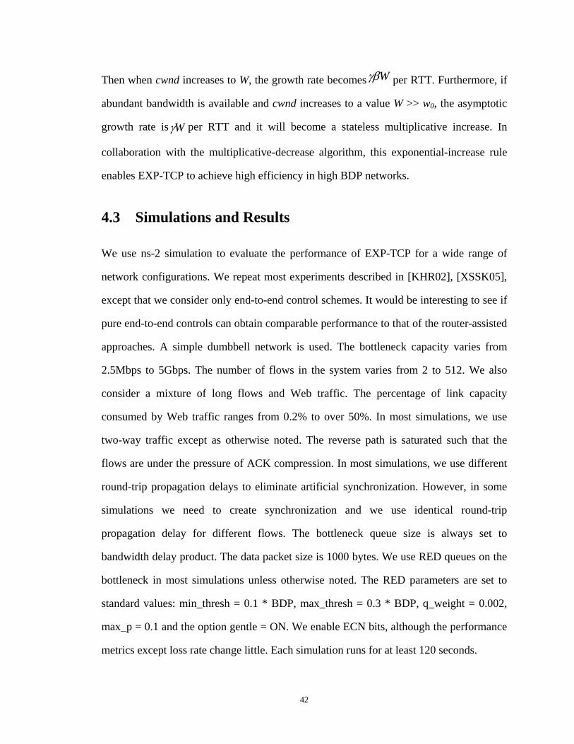
Then when cwnd increases to W, the growth rate becomes Wγβ per RTT. Furthermore, if

abundant bandwidth is available and cwnd increases to a value W >> w0, the asymptotic

growth rate is Wγ per RTT and it will be tateless multiplicative increase. In

collaboration with the multiplicative-decrease algorithm, this exponential-increase rule

enables EXP-TCP to achieve high efficiency in high BDP networks.

We use ns-2 simulation to evaluate the performance of EXP-TCP

come a s

4.3 Si s and Results

for a wide range of

network configurations. We repeat most experiments described in [KHR02], [XSSK05],

trol scheme ould be interesting to see if

mulation

except that we consider only end-to-end con s. It w

pure end-to-end controls can obtain comparable performance to that of the router-assisted

approaches. A simple dumbbell network is used. The bottleneck capacity varies from

2.5Mbps to 5Gbps. The number of flows in the system varies from 2 to 512. We also

consider a mixture of long flows and Web traffic. The percentage of link capacity

consumed by Web traffic ranges from 0.2% to over 50%. In most simulations, we use

two-way traffic except as otherwise noted. The reverse path is saturated such that the

flows are under the pressure of ACK compression. In most simulations, we use different

round-trip propagation delays to eliminate artificial synchronization. However, in some

simulations we need to create synchronization and we use identical round-trip

propagation delay for different flows. The bottleneck queue size is always set to

bandwidth delay product. The data packet size is 1000 bytes. We use RED queues on the

bottleneck in most simulations unless otherwise noted. The RED parameters are set to

standard values: min_thresh = 0.1 * BDP, max_thresh = 0.3 * BDP, q_weight = 0.002,

max_p = 0.1 and the option gentle = ON. We enable ECN bits, although the performance

metrics except loss rate change little. Each simulation runs for at least 120 seconds.

42

Standard TCP, HSTCP, STCP, and our EXP-TCP are compared. The Sack1 variant

is always used and we always set maxburst = 4 according to [FF96]. For HSTCP, we set

all its parameters to their default values (Wlow = 38, Whigh = 83000, Phigh = 0.0000001, and

highβ = 0.1). For STCP, we also set its parameters to the default values (β = 0.125 and

α = 0.01). For EXP-TCP, we set γ =0.05 and β =0.125 for all simulations. All the

simulations are very time-consuming (the ns-2 running time itself is at the order of

s). We are aware of other TCP variants such as BIC-TCP, H-TCP, and FAST-TCP.

e plan to conduct comprehensive evaluation with the configurations described above.

Our hypothesis is that EXP-TCP can achieve a comparable or better performance

while still providing better fairness than HSTCP and STCP. First it should obtain a higher

utilization, smaller queue size and lower drop rate than HSTCP and STCP regardless of

week

W

bottleneck capacity, number of flows, background web traffic size or other network

conditions. Second, it should converge to good fairness faster than HSTCP and STCP in

case of flow competition, and show comparable robustness in response to sudden

considerable traffic changes. To quantify and compare the converge-to-fairness ability of

each algorithm, we use Jain’s fairness index [JCH84] as the metric to evaluate the

simulation results. As a quantitative measure of the fairness of bottleneck bandwidth

allocation, the Jain’s fairness index is defined as follows: for N competing flows with the

throughput xi, Ni ≤≤1 , the fairness index is defined as follows:

∑

∑=

⎟⎠

⎞⎜⎝

⎛

N

i

N

i

xN

x

2

2

1

=i

i

1

4.3.1 Impact of Bottleneck Capacity

In this simulation, we intend to find the impact of bottleneck capacity on EXP-TCP. We

43

vary the bottleneck capacity from 2.5 Mbps to 5 Gbps. In each direction, there are 16

homogeneous flows using the same control algorithm. We create side links with different

propagation delays so that the round-trip propagation delays of the flows are between 60

ms to 100 ms. Each simulation runs for 120 seconds. We obtain (1) the average

every 200 ms, (2) the average queue

the lowest

utiliza

bottleneck utilization, which is an average value in

size normalized by the queue limit which is sampled once every 200 ms, (3) the average

bottleneck drop rate which is calculated for every 200 ms. Moreover, only the results

from the last 100 seconds of the simulation are used for evaluation so as to ensure the

steady state behavior but not the startup transient behavior of TCP is studied.

As shown in Figure 4.2, EXP-TCP consistently achieves more than 95% link

utilization. STCP performs the second best when the capacity is medium but its

utilization drops quickly when the capacity is very high. Since STCP uses MIMD

algorithm, the flow with high throughput keeps grabbing more bandwidth in a more

aggressive manner than the flow with low throughput, which causes the latter to do many

retransmissions and waste much bottleneck bandwidth. Standard TCP obtains

tion when the bottleneck capacity is very high. HSTCP shows the low drop rate,

stable utilization, but its efficiency is lower than that of EXP-TCP and even performs the

worst among four algorithms in some conditions. This is because the aggressiveness of

HSTCP leads to a large burst of packets in the bottleneck queue, so RED drops more

packets to cause the senders to back off too frequently. Finally, all control algorithms

result in low queue size due to the use of RED, but standard TCP results in the lowest

loss, because standard TCP uses AIMD, which is the least aggressive one among all

algorithms.

44

Figure 4. 2 Performance of congestion control algorithms when the bottleneck capacity

ranges from 2.5Mbps to 5.12Gbps

45

4.3.2 Impact of Number of Flows

this simulation, we study the impact of the number of flows. We fix the bottleneck

capacity to 300 Mbps, but range the number of homogeneous flows in each direction

from 2 to 512. All the other configurations are the same as in the previous simulation.

Figure 4.3 shows the simulation results of bottleneck utilization, queue size, and drop

te for each TCP variant. Again we observe that EXP-TCP results in the highest

bottleneck utilization (97%-99%), whereas both standard TCP and HSTCP are much

behind. When the number of flows is small, Standard TCP does poorly, confirming the

ability of standard TCP to grab the abundant bandwidth, while HSTCP performs

ehow better but still not well for medium size capacity, mostly due to its still

dramatic window backoff. When the number of flows is large, HSTCP is almost identical

TCP, since HSTCP is essentially standard TCP when the cwnd is small. STCP has

omparable bottleneck utilization to EXP-TCP when the number of flows is medium (e.g.,

between 20 and 200), but its utilization drops quickly when the number of flows is very

all (e.g., less than 20) or very large (e.g., more than 200). Moreover, although

XP-TCP achieves high efficiency regardless of the number of flows, its average queue

size and drop rate at the bottleneck is still similar to or even lower than that of each other

4.3.3 Impact of Web Traffic

In this simulation, we want to see the impact of short-live web traffic on the performance

f EXP-TCP. We run 16 homogeneous flows in each direction and fix the bottleneck

capacity to 300 Mbps. All the other configurations are the same as the previous two

Pareto distribution with a m eter of 1.35.

In

ra

in

som

to

c

sm

E

TCP variant.

o

simulations. In addition, we introduce short Web-like flows. Their transfer size follows a

ean of 30 packets and a shape param

46

Figure 4. 3 Performance of congestion control algorithms when the number of

long-lived flows ranges from 2 to 512

47

Pe

Web-like flows con ottleneck capacity

Figure 4. 4 rformance of congestion control algorithms when the background

sumes between 2% and 51.2% of the b

48

Figure 4.4 plots the bottleneck utilization, queue size, and drop rate for each

algorithm. It shows that the robustness of EXP-TCP in obtaining good performance

ompared with the other algorithms. TCP is the least aggressive one, as indicated by its

bottleneck queue occupancy and drop rate, but as well as the low utilization. This is

opposite to that of STCP, which stays aggressive, and thus results in high utilization but

lso high queue occupancy and drop rate. HSTCP does poorly on utilization too, which

ight be explained by its dramatic window backoff after bursty losses. In general,

EXP-TCP achieves the highest and stablest bottleneck utilization regardless of the Web

affic consumption of the bottleneck capacity, whereas HSTCP and STCP have clearly

wer bottleneck utilization and their performance fluctuates according to the Web traffic

size. STCP shows comparable bottleneck utilization to EXP-TCP but it has slightly

e bottleneck when compared with EXP-TCP.

4.3.4 Convergence to Fairness

In this simulation, we examine the convergence behavior of various algorithms. We set

e bottleneck capacity to 500 Mbps. Three homogeneous flows will compete for the

her data flows in the other direction. After

the first flow starts at time 0, the second flow joins 100 seconds later and the third flow

ins another 100 seconds later. We run the simulation for 450 seconds such that all the

First, we create a rather synchronized situation. The flows have the identical

round-trip propagation delay of 40 ms, and DropTail is used. For each scenario, the

er-flow throughput is plotted to show the convergence behavior of each flow. We also

alculate Jain’s fairness index for the flow throughput from 200s to 450s to comparison

the , in

which

c

low

a

m

tr

lo

higher queue occupation and drop rate at th

th

bandwidth in one direction but there is not ot

jo

flows which can be converged have enough time to converge.

p

c

converge-to-fairness of each case. Then, we create a less synchronized situation

the round-trip propagation delay varies slightly by 10%, and RED is used.

49

50

Figure 4.5 Convergence to fairness of

competing flows when DropTail is used:

TCP vs. HSTCP vs. STCP vs. EXP-TCP

Figure 4. 6 Convergence to fairness of

competing flows when RED is used: TCP

vs. HSTCP vs. STCP vs. EXP-TCP

Figure 4.5 shows the per-flow throughput (each point is an average value in 200 ms)

when different algorithms are used for the DropTail case. STCP shows the worst

performance. Two flows are starved whereas the first flow does not give up much

ply because the MIMD control has a problem in converging to

fairness. The other three algorithms all manage to converge to fairness with EXP-TCP

converging in a comparable speed to HSTCP although a little slower than TCP.

Figure 4.6 shows the results of the RED case. STCP still have difficulty in

onverging to fairness. Standard TCP exhibits a large fluctuation of cwnd but converges

fairness with the AIMD control. EXP-TCP converges well to fairness with smaller

ariation in throughput than TCP. HSTCP also show convergence but its bandwidth

llocation is less fair than that of EXP-TCP.

Figure 4.7 shows the fairness index of the flow throughput from time 200s to 450s.

s shown in Figure 4.7 (a), STCP shows the lowest fairness while TCP shows the highest

irness as predicted. Importantly, EXP-TCP achieves high fairness comparable to TCP.

STCP shows nearly perfect convergence as opposed to EXP-TCP, but it is slower in

onverging to fairness than EXP-TCP. The fairness index in RED cases is shown in

igure 4.7 (b). STCP is still slow to converge to fairness but has been greatly improved

by the application of RED. EXP-TCP still achieves comparable fairness to TCP and

reaches high fairness faster than HSTCP. However, HSTCP shows more stable fairness

an EXP_TCP.

bandwidth. This is sim

c

to

v

a

A

fa

H

c

F

th

51

(b) RED

Figure 4. 7 Fairness Index: TCP vs. HSTCP vs. STCP vs. EXP-TCP

(a) DropTail

52

4.3.5 Response to Sudden Changes

is simulation, we examine the performance of the algorithms as traffic demands and

ynamics vary considerably. We start the simulation with 10 long-lived flows in each

irection. Their round-trip propagation delays vary between 75 ms and 85 ms. The

ottleneck capacity is 500 Mbps. After 100 seconds, 40 more flows join in the forward

irection. They stay in the system for 100 seconds, and then suddenly leave.

Figure 4.8 shows the change of the average throughput of the ten flows in the

rward direction in response to the sudden changes of the traffic demand. The error bars

tion by showing the standard deviation. The changes of the

bottleneck utilization and bottleneck queue occupation are shown in Figure 4.9 and

Figure 4.10 respectively.

From these plots we can see that standard TCP is the slowest to respond to the

ased availability of bandwidth, and it is unable to reach full utilization at the end of

the simulation run. STCP performs better than standard TCP but its response is still

slower than HSTCP and EXP-TCP in this network settings. Although it uses aggressive

MIMD and thus enjoys high average bandwidth utilization, it still needs more than three

es as long as EXP-TCP to fully utilize the available bandwidth. HSTCP has a

parable response to EXP-TCP but shows two main drawbacks: one is the per-flow

roughput is very unstable, while the other is the average utilization is lower than STCP

nd EXP-TCP. The reason for this lies in its RTT-unfairness problem. EXP-TCP has the

est performance. It is the fastest in ramping up the throughput and utilization. Although

it is not as aggressive as HSTCP n state, it grows more aggressive

when abundant bandwidth is available, and t

bandwidth utilization. On the other hand, EXP-TCP has similar bottleneck queue

occupation to any of the other three algorithms

In th

d

d

b

d

fo

indicate the range of varia

incre

tim

com

th

a

b

and STCP i steady-

hus maintains more stable sending rate and

53

TCP

s. HSTCP vs. STCP vs. EXP-TCP

STCP

Figure 4. 8 Changes of the average throughput of competing flows in response to the

sudden changes of traffic demands: TCP v

HSTCP

EXP-TCP

54

TCP

STCP

HSTCP

EXP-TCP

Figure 4. 9 Changes of bottleneck utilization in response to the sudden changes of

traffic demands: TCP vs. HSTCP vs. STCP vs. EXP-TCP

55

TCP

STCP

Fi s

o

HSTCP

EXP-TCP

gure 4. 10 Changes of bottleneck queue occupation in response to the sudden change

f traffic demands: TCP vs. HSTCP vs. STCP vs. EXP-TCP

56

4.4 Summary

this chapter, we introduced a pure end-to-end congestion control algorithm, EXP-TCP,

which can decouple efficiency control and fairness control so as to effectively overcome

unfairness problem in high BDP networks. EXP-TCP can achieve high efficiency by the

xponential increase in congestion window. Meanwhile, it can also achieve good fairness

by realizing the reasonable relative growth rate among competing flows. We conducted

simulations to evaluate EXP-TCP in various scenarios. Our simulation results have

onfirmed that EXP-TCP can achieve both comparable or better performance and better

nd STCP. It is also suggested by our study that the end-to-end

congestion control algorithms, if properly designed, can perform reasonably well in

chieving high network utilization and low queuing delay with RED queue management.

In

e

c

fairness than HSTCP a

a

57

Chapter 5

and removes the traditional Slow Start phase from TCP while keeping the remainder of

TCP congestion control unchanged. The experimental evaluation and analysis showed

that Jump Start has both positive and negative impacts on the network performance. Jump

Start notably accelerates the transmission when the bottleneck buffer size is not a

hindrance, but suffers from severe problems when multiple drops are caused due to the

over-aggressive initial sending rate.

For the steady-state behavior of TCP, we presented a new end-to-end control

algorithm called EXP-TCP. EXP-TCP replaces the traditional AIMD congestion control

with a stateful EIMD congestion control. The simulation results demonstrated that

EXP-TCP can effectively decouple efficiency control and fairness control in high BDP

networks under various configurations, thus can achieve both high efficiency and good

fairness.

Conclusions and Future Work

5.1 Summary

In this work, we studied the performance of TCP in high BDP networks. For the purpose

of improving both the start-up and steady-state behavior of TCP in high BDP networks,

we made modifications to both Slow Start and Congestion Avoidance algorithms and

implemented them in ns-2 for simulation analysis.

For the start-up behavior of TCP, we introduced a new mechanism named Jump Start.

Jump Start enables the sender to begin transmission at whatever rate it deems appropriate

58

5.2 Future Research

For Jump Start ferent

network setups as well as more realistic traffic patterns, to shed more light on the

Jump Start. Moreover, real-world experiments will also be

important in deepening our understanding of Jump Start. Finally, the security impacts of

For EXP-TCP, further simulation and evaluation under more complex network

conf

, in the future we will further test its performance with dif

implications of using

Jump Start should not be omitted. We will keep an eye on attackers who use Jump Start

to coax some server into sending very high-rate bursts of traffic to facilitate pulsing

attacks.

igurations, such as multiple bottlenecks and a wider range of RTTs, should also be

conducted. In addition, we will compare EXP-TCP with more other end-to-end

algorithms, such as FAST-TCP, BIC-TCP, and H-TCP. Moreover, we will study the

RTT-fairness problem. Finally, we will conduct simulations and experiments to see the

combined effect of Jump Start and EXP-TCP, so as to analyze the pros and cons of their

cooperation.

59

Bibliography

[AD02] G. Asthana and J. Denaro. Gigabit Ethernet: an affordable solution. In

[AP99] M. Allman and V. Paxson. On estimating end-to-end network path

March 2000.

[ATCZ05] L. H. Andrew, L. Tan, T. Cui and M. Zukerman. Fairness comparison of FAST-TCP and TCP Vega . In Proceedings of 19th International Teletraffic Congress, Beijing China, September 2005.

[BA05] E. Blanton and M. Allman. On the impact of bursting on TCP performance. In Passive and Active Measurement Workshop’05, Boston, MA, March 2005.

[BRS99] H. Balakrishnan, H. Rahul, and S. Seshan. An integrated congestion management architecture for Internet hosts. In Proceedings of ACM SIGCOMM’99, Cambridge, MA, September 1999.

[CO02] K. G. Coffman and A. M. Odlyzko. Growth of the Internet. Optical Fiber Telecommunications IV B: Systems and Impairments, pages 17–56, 2002.

Technical Report ECE, Georgia Institute of Technology, January 2002.

[AFP02] M. Allman, S. Floyd, and C. Partridge. Increasing TCP's initial window. RFC 3390, October 2002.

[AHO98] M. Allman, C. Hayes, and S. Ostermann. An evaluation of TCP with larger initial windows. Computer Communication Review, 28(3), March 1998.

properties. In Proceedings of ACM SIGCOMM’99, Cambridge, MA, September 1999.

[APS99] M. Allman, V. Paxson, and W. R. Stevens. TCP congestion control. RFC 2581, April 1999.

[ASA00] A. Aggarwal, S. Savage, and T. Anderson. Understanding the performance of TCP pacing. In Proceedings of IEEE INFOCOM’00, Tel Aviv, Israel,

s

60

[CJ89] D. M. Chiu and R. ncrease and decrease algorithms for congestion avoidance in computer networks. Computer Networks and ISDN Systems, 17(1), June 1989.

[D59] s.

[F03] for large congestion windows. RFC 3649,

[F04] C 3742, Experim

[FAJS06] 006.

uter Communications Review, 26(3), July 1996.

ust 1993.

[JCH84] R. Jain, D. Chiu, and W. Hawe. A quantitative measure of fairness and

[JL07] S. Jin and D. Liu. Decoupling end-to-end efficiency and fairness control in

Jain. Analysis of the i

E. W. Dijkstra. A note on two problems in connection with graphNumerische Mathematik. 1: 269–271, 1959.

S. Floyd. HighSpeed TCPDecember 2003.

S. Floyd. Limited slow-start for TCP with large congestion windows. RFental, March 2004.

S. Floyd, M. Allman, A. Jain, and P. Sarolahti. Quick-Start for TCP and IP. RFC 4782, June 2

[FF96] K. Fall and S. Floyd. Simulation-based comparisons of Tahoe, Reno, and SACK TCP. Comp

[FJ93] S. Floyd and V. Jacobson. Random early detection gateways for congestion avoidance. IEEE/ACM Transactions on Networking, 1(4): 397–413, Aug

[J88] V. Jacobson. Congestion avoidance and control. In Proceedings of the ACM SIGCOMM’88, Palo Alto, CA, August 1988.

discrimination for resource allocation in shared computer systems. DEC Research Report TR-301, September 1984.

high bandwidth-delay product networks. In 5th International Workshop on Protocols for Fast Long-Distance Networks, Marina Del Rey, CA, February 2007.

[JGMB01] S. Jin, L. Guo, I. Matta, and A. Bestavros. TCP-friendly SIMD congestion control and its convergence behavior. In Proceedings of ICNP'01,

61

Riverside, CA, November 2001.

I. Jacobs and N. Walsh. Archit[JW04] ecture of the World Wide Web. W3C Recommendation, December 2004,

[K03] T. Kelly. Scalable TCP: improving performance in highspeed wide area

[K03a] D. Katabi. Decoupling congestion control and bandwidth allocation policy

te of Technology, March 2003.

uct networks. In Proceedings of ACM

[KPW05] ure for

ery. In Proceedings of the ACM SIGCOMM Internet Measurement Workshop’02, Marseille,

[LAJW07] stion control without a startup phase. In 5th International Workshop on Protocols for Fast Long-Distance

[LAW05] airness. In Proceedings of IEEE INFOCOM’05, Miami,

FL, March 2005.

[LPD01]

http://www.w3.org/TR/2004/REC-webarch-20041215

networks. Computer Communication Review, 32(2), April 2003.

with application to high bandwidth-delay product networks. Ph.D. Dissertation, Massachusetts Institu

[KHR02] D. Katabi, M. Handley, and C. Rohrs. Congestion control for high bandwidth-delay prodSIGCOMM’02, Pittsburgh, PA, August 2002.

A. Kumar, V. Paxson, and N. Weaver. Exploiting underlying structdetailed reconstruction of an Internet-scale event. In Proceedings of ACM/USENIX Internet Measurement Conference’05, Berkeley, CA, October 2005.

[KWZ02] B. Krishnamurty, C. Wills, and Y. Zhang. Preliminary measurements on the effect of server adaptation for web content deliv

France, November 2002.

D. Liu, M. Allman, S. Jin, L. Wang. Conge

Networks, Marina Del Rey, CA, February 2007.

S. H. Low, L. Andrew, and B. Wydrowsk. Understanding XCP: equilibrium and f

S. H. Low, F. Paganini, and J. C. Doyle. Internet congestion control: An

62

analytical perspective. IEEE Control Systems Magazine, 2001.

METRICS’01, Cambridge, MA, June

rnational Workshop on Protocols for Fast Long-Distance Networks, Nara, Japan,

[LT04] TCP in Long-Delay Environment. Technical report, Glenn Research Center,

[M95] ted programming in Tcl. In Proceedings of Tcl/Tk Workshop, Berkeley, CA, May 1993.

[MLAW14]

ch 1999.

[NS2]

[NS00] The ns Manual. The VINT project, a collaboration between researchers at

[P80] J. Postel. User datagram protocol. RFC 768, August 1980.

[P81] r, SRI International, September 1981.

5]

[LPW01] S. H. Low, L. Peterson, and L. Wang. Understanding Vegas: a duality model. In Proceedings of ACM SIG2001.

[LS06] D. J. Leith and R. N. Shorten. Impact of drop synchronization on TCP fairness in high bandwidth-delay product networks. In 4th Inte

February 2006.

F. J. Lawas-Grodek and D. T. Tran. Evaluation of Swift Start

Cleveland, OH, October 2004.

Michael J. McLennan. [Incr Tcl] - object orien

J. Mo, R. J. La, V. Anantharam, and J. Walrand. Analysis and comparison of TCP Reno and Vegas. In Proceedings of IEEE INFOCOM ’99, New York, NY, Mar

[MMFR96] M. Mathis, J. Mahdavi, S. Floyd, and A. Romanow. TCP selective acknowledgement options. IETF RFC 2018, October 1996.

Network Simulator 2 (ns-2), available at: http://www.isi.edu/nsnam/ns.

UC Berkeley, LBL, USC/ISI, and Xerox PARC, October 2000, http://www.isi.edu/nsnam/ns/nsdocumentation.html.

I. Postel. Transmission Control Protocol. RFC793, DDN Network Information Cente

[PABLT0 R. Pang, M. Allman, M. Bennett, Jason Lee, and B. Tierney. A first look at

63

modern enterprise traffic. In Proceedings of SIGCOMM/USENIX Internet Measurement Conference’05, Berkeley, CA, October 2005.

[PPP00] proximating fair bandwidth allocation. In Proceedings of IEEE

INFOCOM’00, Tel Aviv, Israel, March 2000.

[PR83]

[PR85] nolds. File transfer protocol (FTP). RFC 959, October 1985.

[PRAKS02] nical Report TR-8339, BBN Technologies,

March 2002.

[SL04] h-speed and long-distance networks. In 2nd International Workshop on Protocols for

[TMW97] iller, and R. Wilder. Wide-area Internet traffic patterns and characteristics. IEEE Network, 11(6):10-23, November 1997.

[WJLH06] P: motivation, architecture, algorithms, performance. IEEE/ACM Transactions on

]

05] Y ne more bit is enough. In Proceedings of ACM SIGCOMM’05, Philadelphia, PA, August

[YLS] T. Yee, D. Leith, and R. Shorten. Experimental evaluation of highspeed

R. Pan, B. Prabhakar, and K. Psounis. CHOKe: a stateless scheme AQM for ap

J. Postel, J. Reynolds. Telnet protocol specification. RFC 854, May 1983.

J. Postel, J. Rey

C. Partridge, D. Rockwell, M. Allman, R. Krishnan, and J. P. G. Sterbenz. A swifter start for TCP. In Tech

R. N. Shorten and D. J. Leith. H-TCP: TCP for hig

Fast Long-Distance Networks, Argonne, IL, February 2004.

K. Thompson, G. J. M

D. X. Wei, C. Jin, S. H. Low and S. Hegde. FAST-TC

Networking, 14(6):1246-1259, December 2006.

[XHR04 L. Xu, K. Harfoush, and I. Rhee. Binary increase congestion control for fast long-distance networks. In Proceedings of IEEE INFOCOM’04, Hongkong, March 2004.

[XSSK . Xia, L. Subramanian, I. Stoica, and S. Kalyanaraman. O

2005.

congestion control protocols. IEEE/ACM Transactions on Networking, to

64

65

[ZSC91] L. Zhang, S. Shenker, and D. Clark. Observations on the dynamics of a

appear.

congestion control algorithm: the effects of two-way traffic. In Proceedings of ACM SIGCOMM’91, Zurich, Switzerland, September 1991.