Improving Software Model Inference by Combining State Merging...
275
The University of Sheffield Doctoral Thesis Improving Software Model Inference by Combining State Merging and Markov Models Author: Abdullah Alsaeedi Supervisor: Dr. Kirill Bogdanov A thesis submitted in fulfilment of the requirements for the degree of Doctor of Philosophy in the Verification and Testing Department of Computer Science April 2016
Transcript of Improving Software Model Inference by Combining State Merging...

The University of Sheffield
Doctoral Thesis
Improving Software Model Inference byCombining State Merging and Markov
Models
Author:
Abdullah Alsaeedi
Supervisor:
Dr. Kirill Bogdanov
A thesis submitted in fulfilment of the requirements
for the degree of Doctor of Philosophy
in the
Verification and Testing
Department of Computer Science
April 2016

THE UNIVERSITY OF SHEFFIELD
Abstract
Faculty of Engineering
Department of Computer Science
Doctor of Philosophy
Improving Software Model Inference by Combining State Merging and
Markov Models
by Abdullah Ahmad Alsaeedi
Labelled-transition systems (LTS) are widely used by developers and testers to model
software systems in terms of their sequential behaviour. They provide an overview of the
behaviour of the system and their reaction to different inputs. LTS models are the founda-
tion for various automated verification techniques such as model-checking and model-based
testing. These techniques require up-to-date models to be meaningful. Unfortunately,
software models are rare in practice. Due to the effort and time required to build these
models manually, a software engineer would want to infer them automatically from traces
(sequences of events or function calls).
Many techniques have focused on inferring LTS models from given traces of system exe-
cution, where these traces are produced by running a system on a series of tests. State-
merging is the foundation of some of the most successful LTS inference techniques to con-
struct LTS models. Passive inference approaches such as k-tail and Evidence-Driven State
Merging (EDSM ) can infer LTS models from these traces. Moreover, the best-performing
methods of inferring LTS models rely on the availability of negatives, i.e. traces that are
not permitted from specific states and such information is not usually available. The long-
standing challenge for such inference approaches is constructing models well from very few
traces and without negatives.
Active inference techniques such as Query-driven State Merging (QSM ) can learn LTSs
from traces by asking queries as tests to a system being learnt. It may lead to infer

ii
inaccurate LTSs since the performance of QSM relies on the availability of traces. The
challenge for such inference approaches is inferring LTSs well from very few traces and
with fewer queries asked.
In this thesis, investigations of the existing techniques are presented to the challenge of
inferring LTS models from few positive traces. These techniques fail to find correct LTS
models in cases of insufficient training data. This thesis focuses on finding better solutions
to this problem by using evidence obtained from the Markov models to bias the EDSM
learner towards merging states that are more likely to correspond to the same state in a
model.
Markov models are used to capture the dependencies between event sequences in the
collected traces. Those dependencies rely on whether elements of event permitted or pro-
hibited to follow short sequences appear in the traces. This thesis proposed EDSM-Markov
a passive inference technique that aimed to improve the existing ones in the absence of
negative traces and to prevent the over-generalization problem. In this thesis, improve-
ments obtained by the proposed learners are demonstrated by a series of experiments
using randomly-generated labelled-transition systems and case studies. The results ob-
tained from the conducted experiments showed that EDSM-Markov can infer better LTSs
compared to other techniques.
This thesis also proposes modifications to the QSM learner to improve the accuracy of the
inferred LTSs. This results in a new learner, which is named ModifiedQSM. This includes
considering more tests to the system being inferred in order to avoid the over-generalization
problem. It includes investigations of using Markov models to reduce the number of
queries consumed by the ModifiedQSM learner. Hence, this thesis introduces a new LTS
inference technique, which is called MarkovQSM. Moreover, enhancements of LTSs inferred
by ModifiedQSM and MarkovQSM learners are demonstrated by a series of experiments.
The results from the experiments demonstrate that ModifiedQSM can infer better LTSs
compared to other techniques. Moreover, MarkovQSM has proven to significantly reduce
the number of membership queries consumed compared to ModifiedQSM with a very small
loss of accuracy.

Acknowledgements
First of all, I would like to thank God for giving me the ability, strength, and patience to
complete this research.
Throughout my life, my parents have supported and encouraged me to study abroad. I
would like to thank them for supporting and believing in me. A special thank to my father
for motivating and believing in me to complete this research. Moreover, my sincere thanks
to my dear wife for her love, and trust in me.
I would like to express my sincere gratitude to my supervisor, Dr. Kirill Bogdanov, for
his advice and continuous support during the four years of this research. He has guided
me relentlessly to complete this thesis. During these years, Kirill has cared about me, and
given me the opportunity to have insightful discussions about the research. He is a very
flexible, supportive and smart person.
iii
Contents
Abstract i
Acknowledgements iii
Contents iv
List of Figures viii
List of Tables xii
1 Introduction 1
1.1 The Importance of Specification Inference . . . . . . . . . . . . . . . . . . . 2
1.1.1 State Machine Inference . . . . . . . . . . . . . . . . . . . . . . . . . 2
1.1.2 Passive Inference and Active Inference . . . . . . . . . . . . . . . . . 5
1.2 Research Motivation . . . . . . . . . . . . . . . . . . . . . . . . . . . . . . . 6
1.3 Aims and Objectives . . . . . . . . . . . . . . . . . . . . . . . . . . . . . . . 7
1.4 Contributions . . . . . . . . . . . . . . . . . . . . . . . . . . . . . . . . . . . 9
1.5 Research Questions . . . . . . . . . . . . . . . . . . . . . . . . . . . . . . . . 9
1.6 Thesis Outline . . . . . . . . . . . . . . . . . . . . . . . . . . . . . . . . . . 10
2 Definitions, Notations, Models, Inference 12
2.1 Deterministic Finite State Automata . . . . . . . . . . . . . . . . . . . . . . 12
2.2 Labelled Transition System . . . . . . . . . . . . . . . . . . . . . . . . . . . 13
2.2.1 LTS and Language . . . . . . . . . . . . . . . . . . . . . . . . . . . . 13
2.2.2 Partial Labelled Transition System . . . . . . . . . . . . . . . . . . . 14
2.2.3 Traces . . . . . . . . . . . . . . . . . . . . . . . . . . . . . . . . . . . 14
2.2.4 Example of Text Editor . . . . . . . . . . . . . . . . . . . . . . . . . 15
2.3 Three Learning-Model Frameworks . . . . . . . . . . . . . . . . . . . . . . . 15
2.3.1 Identification in the Limit . . . . . . . . . . . . . . . . . . . . . . . . 16
2.3.2 Angluin’s Model . . . . . . . . . . . . . . . . . . . . . . . . . . . . . 17
2.3.3 PAC Identification Model . . . . . . . . . . . . . . . . . . . . . . . . 17
2.4 Finite Automata Inference . . . . . . . . . . . . . . . . . . . . . . . . . . . . 18
2.4.1 Preliminaries of finite automata inference . . . . . . . . . . . . . . . 18
2.4.2 The problem of LTS Inference Using Grammar Inference . . . . . . . 18
2.4.3 State Merging . . . . . . . . . . . . . . . . . . . . . . . . . . . . . . . 19
2.4.4 RPNI Algorithm . . . . . . . . . . . . . . . . . . . . . . . . . . . . . 23
2.4.5 Example of RPNI . . . . . . . . . . . . . . . . . . . . . . . . . . . . 25
2.5 Evaluation of Software Models . . . . . . . . . . . . . . . . . . . . . . . . . 26
iv
Contents v
2.5.1 The W-method . . . . . . . . . . . . . . . . . . . . . . . . . . . . . . 26
2.5.2 Comparing Two Models in Terms of Language . . . . . . . . . . . . 30
2.5.3 An Example of a Comparison of the Language of the Inferred Ma-chine to a Reference One . . . . . . . . . . . . . . . . . . . . . . . . 35
2.5.4 Comparing Two Models in Terms of Structure . . . . . . . . . . . . 37
2.5.4.1 LTSDiff Algorithm . . . . . . . . . . . . . . . . . . . . . . 38
2.6 The Evaluation Technique in the Statechum Framework . . . . . . . . . . . 46
2.7 DFA Inference Competitions . . . . . . . . . . . . . . . . . . . . . . . . . . 48
2.7.1 Abbadingo-One Competition . . . . . . . . . . . . . . . . . . . . . . 48
2.7.2 Gowachin Competition . . . . . . . . . . . . . . . . . . . . . . . . . . 49
2.7.3 GECCO Competition . . . . . . . . . . . . . . . . . . . . . . . . . . 49
2.7.4 STAMINA Competition . . . . . . . . . . . . . . . . . . . . . . . . . 49
2.7.5 Zulu Competition . . . . . . . . . . . . . . . . . . . . . . . . . . . . 50
3 Existing Inference Methods 52
3.1 Passive Learning . . . . . . . . . . . . . . . . . . . . . . . . . . . . . . . . . 52
3.1.1 k-tails Algorithm . . . . . . . . . . . . . . . . . . . . . . . . . . . . . 53
3.1.2 Experiments Using k-tails . . . . . . . . . . . . . . . . . . . . . . . . 55
3.1.3 Variants of the k-tails . . . . . . . . . . . . . . . . . . . . . . . . . . 58
3.1.4 Evidence-Driven State Merging . . . . . . . . . . . . . . . . . . . . . 59
3.1.5 Experiments Using EDSM . . . . . . . . . . . . . . . . . . . . . . . . 63
3.1.6 Improvements on EDSM . . . . . . . . . . . . . . . . . . . . . . . . . 67
3.1.7 Other Improvements . . . . . . . . . . . . . . . . . . . . . . . . . . . 69
3.1.8 Introduction of Satisfiability to the State-Merging Strategy . . . . . 70
3.1.9 Heule and Verwer Constraint on State Merging . . . . . . . . . . . . 70
3.1.10 Experiments Using SiccoN . . . . . . . . . . . . . . . . . . . . . . . . 70
3.1.11 DFASAT Algorithm . . . . . . . . . . . . . . . . . . . . . . . . . . . 75
3.1.12 Inferring State-Machine Models by Mining Rules . . . . . . . . . . . 78
3.2 Active Learning . . . . . . . . . . . . . . . . . . . . . . . . . . . . . . . . . . 80
3.2.1 Observation Table . . . . . . . . . . . . . . . . . . . . . . . . . . . . 81
3.2.2 L∗ Algorithm . . . . . . . . . . . . . . . . . . . . . . . . . . . . . . . 81
3.2.3 Example of L∗ . . . . . . . . . . . . . . . . . . . . . . . . . . . . . . 84
3.2.4 Improvements of L∗ in Terms of Handling Counterexamples . . . . . 85
3.2.5 Complexity of L* . . . . . . . . . . . . . . . . . . . . . . . . . . . . . 85
3.2.6 Query-Driven State Merging . . . . . . . . . . . . . . . . . . . . . . 86
3.3 Applications of Active Inference of LTS Models From Traces . . . . . . . . 88
3.3.1 Reverse Engineering LTS Model From Low-Level Traces . . . . . . . 88
3.3.2 Reverse Engineering LTS Model Using LTL Constraints . . . . . . . 89
3.4 Tools of DFA Inference Using Grammar Inference . . . . . . . . . . . . . . . 91
3.4.1 StateChum . . . . . . . . . . . . . . . . . . . . . . . . . . . . . . . . 91
3.4.2 The LearnLib Tool . . . . . . . . . . . . . . . . . . . . . . . . . . . . 91
3.4.3 Libalf . . . . . . . . . . . . . . . . . . . . . . . . . . . . . . . . . . . 91
3.4.4 Gitoolbox . . . . . . . . . . . . . . . . . . . . . . . . . . . . . . . . . 91
3.5 The Performance of Existing Techniques From Few Long Traces . . . . . . 92
4 Improvement of EDSM Inference Using Markov Models 96

Contents vi
4.1 Introduction . . . . . . . . . . . . . . . . . . . . . . . . . . . . . . . . . . . . 97
4.2 Cook and Wolf Markov Learner . . . . . . . . . . . . . . . . . . . . . . . . . 98
4.3 The Proposed Markov Models . . . . . . . . . . . . . . . . . . . . . . . . . . 100
4.3.1 Building the Markov Table . . . . . . . . . . . . . . . . . . . . . . . 100
4.3.2 Markov Predictions for a Given State . . . . . . . . . . . . . . . . . 103
4.3.3 The Precision and Recall of the Markov Model . . . . . . . . . . . . 104
4.3.4 Definitions of Precision and Recall for Markov Models . . . . . . . . 104
4.3.5 Markov Precision and Recall . . . . . . . . . . . . . . . . . . . . . . 105
4.4 EDSM-Markov . . . . . . . . . . . . . . . . . . . . . . . . . . . . . . . . . . 107
4.4.1 Inconsistency Score (Incons) . . . . . . . . . . . . . . . . . . . . . . 107
4.4.1.1 Inconsistency Score for a Specific State . . . . . . . . . . . 108
4.4.1.2 Inconsistency Score for an Automaton . . . . . . . . . . . . 111
4.4.2 Inconsistency Heuristic for State Merging . . . . . . . . . . . . . . . 111
4.4.3 EDSM-Inconsistency Heuristic . . . . . . . . . . . . . . . . . . . . . 114
4.4.4 EDSM-Markov Inference Algorithm . . . . . . . . . . . . . . . . . . 118
4.5 Summary of the Chapter . . . . . . . . . . . . . . . . . . . . . . . . . . . . . 121
5 Experimental Evaluation and Case Studies of EDSM-Markov 122
5.1 Introduction . . . . . . . . . . . . . . . . . . . . . . . . . . . . . . . . . . . . 122
5.2 Experimental Evaluation of the EDSM-Markov Algorithms . . . . . . . . . 123
5.2.1 Methodology . . . . . . . . . . . . . . . . . . . . . . . . . . . . . . . 123
5.2.2 Main Results . . . . . . . . . . . . . . . . . . . . . . . . . . . . . . . 125
5.2.3 The Impact of the Number of Traces on the Performance of EDSM-Markov . . . . . . . . . . . . . . . . . . . . . . . . . . . . . . . . . . 127
5.2.4 The Impact of Alphabet Size on the Performance of EDSM-Markov 131
5.2.5 The Impact of the Length of Traces on the Performance of EDSM-Markov . . . . . . . . . . . . . . . . . . . . . . . . . . . . . . . . . . 136
5.2.5.1 When m = 2.0 . . . . . . . . . . . . . . . . . . . . . . . . . 137
5.2.5.2 When m = 0.5 . . . . . . . . . . . . . . . . . . . . . . . . . 140
5.2.5.3 When m = 1.0 . . . . . . . . . . . . . . . . . . . . . . . . . 144
5.2.6 The Impact of Prefix Length on the Performance of EDSM-Markov 146
5.3 Case Studies . . . . . . . . . . . . . . . . . . . . . . . . . . . . . . . . . . . 151
5.3.1 Case Study: SSH Protocol . . . . . . . . . . . . . . . . . . . . . . . . 152
5.3.2 Case Study: Mine Pump . . . . . . . . . . . . . . . . . . . . . . . . . 157
5.3.3 Case Study: CVS Client . . . . . . . . . . . . . . . . . . . . . . . . . 161
5.4 Discussion . . . . . . . . . . . . . . . . . . . . . . . . . . . . . . . . . . . . . 167
5.5 Threats to Validity . . . . . . . . . . . . . . . . . . . . . . . . . . . . . . . . 169
5.6 Conclusions . . . . . . . . . . . . . . . . . . . . . . . . . . . . . . . . . . . . 169
6 Improvements to the QSM Algorithm 171
6.1 Introduction . . . . . . . . . . . . . . . . . . . . . . . . . . . . . . . . . . . . 171
6.2 The Proposed Query Generators . . . . . . . . . . . . . . . . . . . . . . . . 173
6.2.1 Dupont’s QSM Queries . . . . . . . . . . . . . . . . . . . . . . . . . 173
6.2.2 One-step Generator . . . . . . . . . . . . . . . . . . . . . . . . . . . 175
6.3 The Modified QSM . . . . . . . . . . . . . . . . . . . . . . . . . . . . . . . . 177
6.3.1 Processing Membership Queries . . . . . . . . . . . . . . . . . . . . . 180

Contents vii
6.4 Introduction of Markov Predictions to the ModifiedQSM Algorithm . . . . . 182
6.4.1 Updating the Markov Matrix . . . . . . . . . . . . . . . . . . . . . . 183
6.4.2 The ModifiedQSM With Markov Predictions . . . . . . . . . . . . . 188
6.5 Conclusion . . . . . . . . . . . . . . . . . . . . . . . . . . . . . . . . . . . . 189
7 Experimental Evaluation of ModifiedQSM and MarkovQSM 192
7.1 Introduction . . . . . . . . . . . . . . . . . . . . . . . . . . . . . . . . . . . . 192
7.2 Experimental Setup and Evaluation . . . . . . . . . . . . . . . . . . . . . . 193
7.2.1 Evaluating the Performance of ModifiedQSM and MarkovQSMin Terms of BCR Scores . . . . . . . . . . . . . . . . . . . . . . . . . 194
7.2.2 Evaluating the Performance of ModifiedQSM and MarkovQSMin Terms of Structural-Similarity Scores . . . . . . . . . . . . . . . . 196
7.2.3 Number of Membership Queries . . . . . . . . . . . . . . . . . . . . . 199
7.3 Case Studies . . . . . . . . . . . . . . . . . . . . . . . . . . . . . . . . . . . 205
7.3.1 Case Study: SSH Protocol . . . . . . . . . . . . . . . . . . . . . . . . 205
7.3.2 Case Study: Mine Pump . . . . . . . . . . . . . . . . . . . . . . . . . 211
7.3.3 Case Study: CVS Client . . . . . . . . . . . . . . . . . . . . . . . . . 217
7.4 Discussion . . . . . . . . . . . . . . . . . . . . . . . . . . . . . . . . . . . . . 224
7.5 Threats to Validity . . . . . . . . . . . . . . . . . . . . . . . . . . . . . . . . 226
7.6 Conclusion . . . . . . . . . . . . . . . . . . . . . . . . . . . . . . . . . . . . 227
8 Conclusion and Future Work 228
8.1 Introduction . . . . . . . . . . . . . . . . . . . . . . . . . . . . . . . . . . . . 228
8.2 Summary of Thesis and Achievements . . . . . . . . . . . . . . . . . . . . . 229
8.3 Contributions . . . . . . . . . . . . . . . . . . . . . . . . . . . . . . . . . . . 230
8.4 Research Questions . . . . . . . . . . . . . . . . . . . . . . . . . . . . . . . . 231
8.5 Limitations and Future Work . . . . . . . . . . . . . . . . . . . . . . . . . . 233
8.5.1 Possible Improvements to EDSM-Markov . . . . . . . . . . . . . . . 233
8.5.1.1 Finding Multiple Solutions . . . . . . . . . . . . . . . . . . 234
8.5.1.2 Mining Rules from the Traces . . . . . . . . . . . . . . . . 235
8.5.2 Possible Improvements to ModifiedQSM and MarkovQSM . . . . . . 235
8.6 Thesis Conclusion . . . . . . . . . . . . . . . . . . . . . . . . . . . . . . . . 236
A Appendix of inferred model evaluation 237
A.1 Test sequences generated for the text editor example . . . . . . . . . . . . . 237
Bibliography 241

List of Figures
2.1 An LTS of a text editor . . . . . . . . . . . . . . . . . . . . . . . . . . . . . 15
2.2 A PTA of a text editor . . . . . . . . . . . . . . . . . . . . . . . . . . . . . . 20
2.3 An APTA of a text editor . . . . . . . . . . . . . . . . . . . . . . . . . . . . 21
2.4 An example of state merging . . . . . . . . . . . . . . . . . . . . . . . . . . 21
2.5 An LTS obtained by merging of C and G . . . . . . . . . . . . . . . . . . . 23
2.6 An example of PTA for a text editor . . . . . . . . . . . . . . . . . . . . . . 25
2.7 An automaton after the merging of states A and B . . . . . . . . . . . . . . 25
2.8 The reference LTS and the mined one of the text editor example . . . . . . 36
2.9 Comparing the reference LTS and the mined one of the text editor exampleusing the LTSDiff Algorithm . . . . . . . . . . . . . . . . . . . . . . . . . . 45
2.10 The output of LTSDiff between the reference LTS 2.9(a) and the inferredLTS 2.9(b) of a text editor example . . . . . . . . . . . . . . . . . . . . . . . 45
2.11 The evaluation framework in Statechum . . . . . . . . . . . . . . . . . . . . 47
3.1 A PTA of text editor from positive samples . . . . . . . . . . . . . . . . . . 54
3.2 A non-deterministic machine after merging pairs of states (A,D) and (H,E) 54
3.3 A machine of text editor where K=1 . . . . . . . . . . . . . . . . . . . . . . 54
3.4 Structural-similarity scores of LTSs inferred using the k -tails algorithm fordifferent k values . . . . . . . . . . . . . . . . . . . . . . . . . . . . . . . . . 57
3.5 BCR scores of LTSs inferred by the k -tails algorithm for different k values . 57
3.6 A PTA in the red-blue algorithm . . . . . . . . . . . . . . . . . . . . . . . . 61
3.7 BCR scores obtained using the EDSM algorithm for different EDSM thresh-old values . . . . . . . . . . . . . . . . . . . . . . . . . . . . . . . . . . . . . 64
3.8 Structural-similarity scores of LTSs inferred using the EDSM algorithm fordifferent EDSM threshold values . . . . . . . . . . . . . . . . . . . . . . . . 65
3.9 Ratio of correctness for the number of states of learnt LTSs using differentEDSM learners from positive samples only . . . . . . . . . . . . . . . . . . . 67
3.10 Ratio of correctness for the number of states of learnt LTSs using differentEDSM learners from positive and negative samples . . . . . . . . . . . . . . 68
3.11 An example of Sicco’s idea . . . . . . . . . . . . . . . . . . . . . . . . . . . . 71
3.12 BCR of LTSs inferred using SiccoN and different EDSM learners from pos-itive sequences only . . . . . . . . . . . . . . . . . . . . . . . . . . . . . . . 71
3.13 BCR attained by SiccoN and different EDSM learners from positive andnegative sequences . . . . . . . . . . . . . . . . . . . . . . . . . . . . . . . . 72
3.14 Structural-similarity scores achieved by SiccoN and different EDSM learnersfrom positive sequences only . . . . . . . . . . . . . . . . . . . . . . . . . . . 73
3.15 Structural-similarity scores achieved by SiccoN and different EDSM learnersfrom positive sequences and negative . . . . . . . . . . . . . . . . . . . . . . 73
viii

List of Figures ix
3.16 Ratio of correctness for the number of states of learnt LTSs using SiccoNvs. different EDSM learners from positive samples only . . . . . . . . . . . 74
3.17 Ratio of correctness for the number of states of learnt LTSs using SiccoNvs. different EDSM learners from positive and negative samples . . . . . . . 75
3.18 Pre-merge of B and C . . . . . . . . . . . . . . . . . . . . . . . . . . . . . . 88
3.19 Post-merge of B and C . . . . . . . . . . . . . . . . . . . . . . . . . . . . . . 88
3.20 BCR scores attained by different learners where the number of traces is 7and the length of traces is given by = 0.5× |Q| × |Σ| . . . . . . . . . . . . . 92
3.21 Structural-similarity scores attained by different learners where the numberof traces is 7 and the length of traces is given by = 0.5× |Q| × |Σ| . . . . . 93
3.22 BCR scores of LTSs inferred using QSM . . . . . . . . . . . . . . . . . . . . 94
3.23 Structural-similarity attained by QSM . . . . . . . . . . . . . . . . . . . . . 95
3.24 Number of membership queries asked by QSM . . . . . . . . . . . . . . . . 95
4.1 The event graph generated from the first-order table . . . . . . . . . . . . . 99
4.2 An LTS of a text editor . . . . . . . . . . . . . . . . . . . . . . . . . . . . . 107
4.3 Example of computing Inconsq . . . . . . . . . . . . . . . . . . . . . . . . . 109
4.4 The initial PTA of a text editor example . . . . . . . . . . . . . . . . . . . . 113
4.5 LTS obtained by merging B and C . . . . . . . . . . . . . . . . . . . . . . . 113
4.6 LTS obtained by merging D and K . . . . . . . . . . . . . . . . . . . . . . . 114
4.7 BCR scores obtained by EDSM-Markov for different inconsistency multi-plier Incon . . . . . . . . . . . . . . . . . . . . . . . . . . . . . . . . . . . . 116
4.8 Structural-similarity scores obtained by EDSM-Markov for different incon-sistency multiplier Incon . . . . . . . . . . . . . . . . . . . . . . . . . . . . 117
4.9 The first example of inconsistency score computation . . . . . . . . . . . . . 118
4.10 The second example of inconsistency score computation . . . . . . . . . . . 118
5.1 Bagplot of BCR scores attained by EDSM-Markov and SiccoN for a five trace126
5.2 Bagplot of structural-similarity scores attained by EDSM-Markov and Sic-coN for a five trace . . . . . . . . . . . . . . . . . . . . . . . . . . . . . . . . 126
5.3 A boxplot of BCR scores attained by EDSM-Markov and SiccoN for adifferent number of traces (T ) . . . . . . . . . . . . . . . . . . . . . . . . . . 127
5.4 Improvement ratio of BCR scores achieved by EDSM-Markov to SiccoN . . 128
5.5 A boxplot of structural-similarity scores attained by EDSM-Markov andSiccoN for a different number of traces . . . . . . . . . . . . . . . . . . . . . 129
5.6 Improvement ratio of structural-similarity scores achieved by EDSM-Markovto SiccoN . . . . . . . . . . . . . . . . . . . . . . . . . . . . . . . . . . . . . 130
5.7 BCR scores obtained by EDSM-Markov and SiccoN for different alphabetmultiplier m in |Σ| = m ∗ |Q| . . . . . . . . . . . . . . . . . . . . . . . . . . 132
5.8 Improvement ratio of BCR scores achieved by EDSM-Markov to SiccoN fordifferent alphabet multiplier and various number of traces . . . . . . . . . . 133
5.9 Accuracy of Markov predictions for a different alphabet multiplier acrossvarious number of traces . . . . . . . . . . . . . . . . . . . . . . . . . . . . . 134
5.10 Structural-similarity scores of EDSM-Markov and SiccoN for different al-phabet multiplier m in |Σ| = m ∗ |Q| . . . . . . . . . . . . . . . . . . . . . . 134
5.11 Improvement ratio of structural-similarity scores achieved by EDSM-Markovto SiccoN for different alphabet multiplier and various number of traces . . 135

List of Figures x
5.12 Blots of BCR scores obtained by EDSM-Markov and SiccoN for differentsetting of l and various numbers of traces where m = 2.0, the length oftraces is given by = l ∗ 2 ∗ |Q|2 . . . . . . . . . . . . . . . . . . . . . . . . . 137
5.13 Transition coverage for different setting of l and various numbers of traceswhere m = 2.0 and the length of traces is given by = l ∗ 2 ∗ |Q|2 . . . . . . 138
5.14 Structural-similarity scores obtained by EDSM-Markov and SiccoN for dif-ferent l, l ∗ |Q| ∗ |Σ| = 2 ∗ l ∗ |Q|2 . . . . . . . . . . . . . . . . . . . . . . . . 139
5.15 BCR scores obtained by EDSM-Markov and SiccoN for different l wherem = 0.5, = l ∗ 2 ∗ |Q|2 . . . . . . . . . . . . . . . . . . . . . . . . . . . . . . 141
5.16 Structural-similarity scores obtained by EDSM-Markov and SiccoN for dif-ferent l where m = 0.5, = l ∗ 2 ∗ |Q|2 . . . . . . . . . . . . . . . . . . . . . . 141
5.17 BCR scores obtained by EDSM-Markov and SiccoN for different setting ofl and various numbers of traces where m = 1.0 and the length of traces isgiven by = l ∗ 2 ∗ |Q|2 . . . . . . . . . . . . . . . . . . . . . . . . . . . . . . 144
5.18 structural difference scores obtained by EDSM-Markov for trace length mul-tiplier l setting the length of each of the 5 traces to l ∗ |Q| ∗ |Σ| = 2 ∗ l ∗ |Q|2 145
5.19 BCR scores for EDSM-Markov and SiccoN for a different prefix length, andvarious number of traces . . . . . . . . . . . . . . . . . . . . . . . . . . . . . 147
5.20 Accuracy of Markov predictions for a different prefix length across differentnumber of traces . . . . . . . . . . . . . . . . . . . . . . . . . . . . . . . . . 148
5.21 EDSM-Markov v.s. SiccoN for a different prefix length,ratio of BCR scores 149
5.22 Number of inconsistency of the trained Markov with comparison to thetarget model . . . . . . . . . . . . . . . . . . . . . . . . . . . . . . . . . . . 150
5.23 structural difference scores attained by EDSM-Markov for a different prefixlength and various numbers of traces . . . . . . . . . . . . . . . . . . . . . . 150
5.24 BCR scores of SSH Protocol case study . . . . . . . . . . . . . . . . . . . . 153
5.25 structural-similarity scores of SSH Protocol case study . . . . . . . . . . . . 154
5.26 Markov precision and recall scores of SSH Protocol case study . . . . . . . . 155
5.27 Inconsistencies of SSH protocol case study . . . . . . . . . . . . . . . . . . . 156
5.28 BCR scores of water mine pump case study . . . . . . . . . . . . . . . . . . 157
5.29 structural-similarity scores of water mine pump case study . . . . . . . . . . 159
5.30 Markov precision and recall scores of water mine case study . . . . . . . . . 161
5.31 Inconsistencies of water mine case study . . . . . . . . . . . . . . . . . . . . 162
5.32 BCR scores of CVS protocol case study . . . . . . . . . . . . . . . . . . . . 163
5.33 Structural-similarity scores of CVS protocol case study . . . . . . . . . . . . 164
5.34 Markov precision and recall scores of water mine case study . . . . . . . . . 165
5.35 Inconsistencies of CVS case study . . . . . . . . . . . . . . . . . . . . . . . . 166
6.1 The first example of computing the Dupontqueries . . . . . . . . . . . . . . 174
6.2 The second example of computing the Dupontqueries . . . . . . . . . . . . 175
6.3 An example of computing the one-step generator . . . . . . . . . . . . . . . 176
6.4 An example of updating a PTA . . . . . . . . . . . . . . . . . . . . . . . . . 182
6.5 The automaton before asking queries . . . . . . . . . . . . . . . . . . . . . . 186
6.6 The automaton after merging B and D . . . . . . . . . . . . . . . . . . . . 186
6.7 The automaton before asking queries . . . . . . . . . . . . . . . . . . . . . . 187

List of Figures xi
7.1 Boxplots of BCR scores achieved by various learners for different setting ofm and T . . . . . . . . . . . . . . . . . . . . . . . . . . . . . . . . . . . . . . 195
7.2 Boxplots of structural-similarity scores attained by ModifiedQSM, MarkovQSM,and QSM learners for different setting of m and T . . . . . . . . . . . . . . 197
7.3 The number of membership queries that were asked by different learnerswhen m = 0.5 . . . . . . . . . . . . . . . . . . . . . . . . . . . . . . . . . . . 199
7.4 The number of membership queries that were asked by different learnerswhen m = 1.0 . . . . . . . . . . . . . . . . . . . . . . . . . . . . . . . . . . . 200
7.5 The number of membership queries that were asked by different learnerswhen m = 2.0 . . . . . . . . . . . . . . . . . . . . . . . . . . . . . . . . . . . 202
7.6 The transition cover of the generated traces . . . . . . . . . . . . . . . . . . 203
7.7 The precision and recall of the Markov model . . . . . . . . . . . . . . . . . 204
7.8 The BCR scores attained by ModifiedQSM, MarkovQSM, and QSM for theSSH protocol case study . . . . . . . . . . . . . . . . . . . . . . . . . . . . . 205
7.9 The structural-similarity scores attained by ModifiedQSM, MarkovQSM,and QSM for the SSH protocol case study . . . . . . . . . . . . . . . . . . . 207
7.10 The number of membership queries of different learners . . . . . . . . . . . 208
7.11 Transition coverage of SSH Protocol case study . . . . . . . . . . . . . . . . 210
7.12 Markov precision and recall scores of SSH Protocol case study . . . . . . . . 210
7.13 Inconsistencies of SSH protocol case study . . . . . . . . . . . . . . . . . . . 211
7.14 BCR scores of water mine pump case study . . . . . . . . . . . . . . . . . . 212
7.15 Structural-similarity scores of water mine pump case study . . . . . . . . . 213
7.16 The number of membership queries of different learners for water mine casestudt . . . . . . . . . . . . . . . . . . . . . . . . . . . . . . . . . . . . . . . . 214
7.17 Transition coverage of water mine case study . . . . . . . . . . . . . . . . . 216
7.18 Markov precision and recall scores of water mine case study . . . . . . . . . 216
7.19 Inconsistencies of water mine case study . . . . . . . . . . . . . . . . . . . . 217
7.20 BCR scores of CVS protocol case study . . . . . . . . . . . . . . . . . . . . 218
7.21 Structural-similarity scores of CVS protocol case study . . . . . . . . . . . . 219
7.22 The number of membership queries of different learners for water mine casestudy . . . . . . . . . . . . . . . . . . . . . . . . . . . . . . . . . . . . . . . 221
7.23 Transition coverage of CVS case study . . . . . . . . . . . . . . . . . . . . . 222
7.24 Markov precision and recall scores of CVS case study . . . . . . . . . . . . . 223
7.25 Inconsistencies of CVS case study . . . . . . . . . . . . . . . . . . . . . . . . 224

List of Tables
2.1 Conventional manner of classifying sequences into relevant and retrieved sets 32
2.2 Refined-way of classifying sequences into relevant and retrieved sets . . . . 33
2.3 Refined-way of computing the precision and recall . . . . . . . . . . . . . . 33
2.4 Confusion matrix for binary classification of sequences . . . . . . . . . . . . 34
2.5 Different metrics for comparing two LTS in terms of their languages . . . . 35
2.6 Confusion matrix for binary classification of sequences . . . . . . . . . . . . 36
2.7 Metrics scores obtained from confusion matrix . . . . . . . . . . . . . . . . 37
2.8 Example of the similarity score computation . . . . . . . . . . . . . . . . . . 39
3.1 An example of the observation table . . . . . . . . . . . . . . . . . . . . . . 81
3.2 The first round of learning DFA M using the L∗ algorithm . . . . . . . . . 84
4.1 The First- and Second-order probability table of text editor example . . . . 99
4.2 The First- and Second-order event-sequence table of text editor example . . 101
4.3 Markov table . . . . . . . . . . . . . . . . . . . . . . . . . . . . . . . . . . . 107
4.4 Classification of inconsistency . . . . . . . . . . . . . . . . . . . . . . . . . . 110
4.5 The Markov Table where k = 2 . . . . . . . . . . . . . . . . . . . . . . . . . 110
4.6 Classification of inconsistency for the prefix path 〈Load,Close〉 and state B 111
5.1 p-values obtained using the Wilcoxon signed-rank test for the main results . 127
5.2 p-values obtained using the Wilcoxon signed-rank test of comparing EDSM-Markov v.s. SiccoN across different number of traces . . . . . . . . . . . . . 131
5.3 Wilcoxon signed rank test with continuity correction of comparing EDSM-Markov v.s. SiccoN using various alphabet multiplier . . . . . . . . . . . . 136
5.4 p-values obtained using the Wilcoxon signed-rank test by comparing EDSM-Markov v.s. SiccoN across different number of traces where m=2.0 . . . . . 140
5.5 p-values obtained using the Wilcoxon signed-rank test by comparing EDSM-Markov v.s. SiccoN across different numbers of traces where m=0.5 . . . . 143
5.6 p-values obtained using the Wilcoxon signed-rank test by comparing EDSM-Markov v.s. SiccoN across different numbers of traces where m=1.0 . . . . 146
5.7 p-values obtained using the Wilcoxon signed rank test for different prefixlength . . . . . . . . . . . . . . . . . . . . . . . . . . . . . . . . . . . . . . . 151
5.8 p-values obtained using the Wilcoxon signed-rank test of SSH protocol casestudy for BCR scores . . . . . . . . . . . . . . . . . . . . . . . . . . . . . . . 152
5.9 p-values obtained using the Wilcoxon signed-rank test of the structural-similarity scores for the SSH protocol case study . . . . . . . . . . . . . . . 155
5.10 p-values of Wilcoxon signed rank test of water mine case study for BCRscores . . . . . . . . . . . . . . . . . . . . . . . . . . . . . . . . . . . . . . . 158
xii
List of Tables xiii
5.11 p-values of Wilcoxon signed rank test of water mine case study for structural-similarity Scores . . . . . . . . . . . . . . . . . . . . . . . . . . . . . . . . . 160
5.12 p-values of Wilcoxon signed rank test of CVS case study for BCR scores . . 162
5.13 p-values of Wilcoxon signed rank test of CVS case study for structural-similarity scores . . . . . . . . . . . . . . . . . . . . . . . . . . . . . . . . . . 165
6.1 An example of updating the Markov table when k = 1 . . . . . . . . . . . . 186
6.2 An example of updating the Markov table when k = 2 . . . . . . . . . . . . 187
7.1 The median values of BCR scores obtained by ModifiedQSM, MarkovQSM,and QSM . . . . . . . . . . . . . . . . . . . . . . . . . . . . . . . . . . . . . 195
7.2 The p-values obtained using the Wilcoxon signed-rank test for differentcomparisons of the BCR scores attained by ModifiedQSM, MarkovQSM,and QSM . . . . . . . . . . . . . . . . . . . . . . . . . . . . . . . . . . . . . 196
7.3 The median values of structural-similarity scores attained by ModifiedQSM,MarkovQSM, and QSM . . . . . . . . . . . . . . . . . . . . . . . . . . . . . 197
7.4 The p-values obtained using the Wilcoxon signed-rank test for differentcomparisons of the structural-similarity scores attained by ModifiedQSM,MarkovQSM, and QSM . . . . . . . . . . . . . . . . . . . . . . . . . . . . . 198
7.5 The median values of number of membership queries when m = 0.5 . . . . . 200
7.6 The p-values obtained using the Wilcoxon signed-rank test for differentcomparisons of the number of membership queries when m = 0.5 . . . . . . 200
7.7 The median values of number of membership queries when m = 1.0 . . . . . 201
7.8 The p-values obtained using the Wilcoxon signed-rank test for differentcomparisons of the number of membership queries when m = 1.0 . . . . . . 201
7.9 The median values of number of membership queries . . . . . . . . . . . . . 202
7.10 The p-values obtained using the Wilcoxon signed-rank test for differentcomparisons of the number of membership queries . . . . . . . . . . . . . . 202
7.11 p-values obtained using the Wilcoxon signed-rank test after comparing theBCR scores attained by ModifiedQSM, MarkovQSM, and QSM for the SSHprotocol case study . . . . . . . . . . . . . . . . . . . . . . . . . . . . . . . . 206
7.12 p-values obtained using the Wilcoxon signed-rank test after comparing thestructural-similarity scores attained by ModifiedQSM, MarkovQSM, andQSM for the SSH protocol case study . . . . . . . . . . . . . . . . . . . . . 207
7.13 p-values obtained by the Wilcoxon signed-rank test of structural-similarityscores for SSH protocol case study . . . . . . . . . . . . . . . . . . . . . . . 209
7.14 p-values of the Wilcoxon signed-rank test of BCR scores for water mine casestudy . . . . . . . . . . . . . . . . . . . . . . . . . . . . . . . . . . . . . . . 212
7.15 p-values of Wilcoxon signed rank test of water mine case study for structural-similarity Scores . . . . . . . . . . . . . . . . . . . . . . . . . . . . . . . . . 213
7.16 p-values obtained by the Wilcoxon signed-rank test of number of member-ship queries for water mine case study . . . . . . . . . . . . . . . . . . . . . 215
7.17 p-values of Wilcoxon signed-rank test of BCR scores for the CVS case study 218
7.18 p-values of Wilcoxon signed rank test of CVS case study for structural-similarity scores . . . . . . . . . . . . . . . . . . . . . . . . . . . . . . . . . . 220
7.19 p-values obtained by the Wilcoxon signed-rank test of numbers of queriesfor CVS case study . . . . . . . . . . . . . . . . . . . . . . . . . . . . . . . . 222
List of Tables xiv
A.1 The set of tests and the corresponding classification using the reference LTSand the inferred LTS . . . . . . . . . . . . . . . . . . . . . . . . . . . . . . . 237

“Even perfect program verification can only establish that a program
meets its specification. The hardest part of the software task is arriv-
ing at a complete and consistent specification, and much of the essence
of building a program is in fact the debugging of the specification.”
Brooks (1987)
1Introduction
Software specifications are vital at varying stages during the development of software
systems. A software specification is a description of the behaviours of the system under
development. Specifications can be formal and informal. Formal specifications are based
on a mathematical basis, represented in formal methods such as Z notations [1]. Informal
specifications are usually presented in a readable form such as natural language or visual
descriptions, and they are included to ease the comprehension of software systems.
In practice, specifications are difficult to write and to modify manually [2, 3]. Brooks [4]
claimed that the hardest part during the development of a system is identifying a complete
specification.
1

Chapter 1. Introduction 2
1.1 The Importance of Specification Inference
The importance of complete and up-to-date specifications is becoming necessary for pro-
gram comprehension, validation, maintenance, and verification techniques [5, 6]. Mainte-
nance costs can be high if specification missing or outdated [7]. Hence, the existence of
up-to-date specifications can reduce maintenance costs [6].
Indeed, complete specifications can aid test generation techniques [8]. Tests can be gener-
ated from specifications. However, tests may be worthless if the quality of specifications
are poor [9]. Therefore, testing strategies require the complete specification of a system to
understand its behaviours and to run meaningful tests that can detect failures easily [8].
Thus, the correctness and reliability of the system are increased.
Today, most software systems are developed with incomplete specifications [20] since de-
velopers focus on developing software rather than keeping complete and up-to-date doc-
umentations [6]. This negatively affects the program comprehension needed by software
engineers to understand the correct behaviours. Therefore, software maintenance can be
costly if specifications are outdated or incomplete [2, 21].
To resolve the issue of imprecise and out-dated specifications, the term specification mining
(inference) has been introduced to increase the program comprehension [22]. Specification
mining can be defined as the automatic process of inferring (extracting) specification
as rules [23–26] or behavioural models [22, 27, 28] for a software system. In general,
specifications can be inferred from source code [29–31], test cases [32, 33], or execution
traces [22, 27, 28].
Ammons et al. [22] stated that automatically extracting specifications can aid verification
and enhance the quality of software. However, existing specification inference approaches
may produce imprecise specifications [22].
1.1.1 State Machine Inference
In the previous section, the importance of inferring specification is described. In this sec-
tion, a finite state machine (FSM) and labelled transitions systems (LTS) are introduced.
After that, state-based specification inference is described. LTS models are widely used for
Chapter 1. Introduction 3
verification and validation techniques. In this thesis, we focus on inferring state machine
specifications, especially LTS, using the state-merging strategy.
A FSM [10] is a model that is often used to represent a software system, and provides a
high-level overview of a system. A FSM is used widely to represent specifications [11]. The
state-machine model of a system consists of a set of states and transitions. Each state is
represented visually by a circled node where a system may be in. Transitions are linking
states to each other, so the system can change its state by moving from its current state to
another one if there is a transition between them and this trigged by a specific event [10].
Transitions are shown as edges (arrows).
LTS [12] are an instance of a state machine often used to model system behaviour, and
are relied upon by many verification and testing techniques. An LTS model is a simple
structure of state machine consisting of states, transitions, and action labels. Behaviours
of software systems are often ordered sequences of events or function calls, and can be
represented using LTS models [13].
The importance of state-machine models arises in various stages during software develop-
ment. Testing is one of the most crucial phases to ensure the quality of software systems
during their development. It is well known that state machine models play a vital role in
testing software system. For instance, model-based testing generation techniques benefit
from behavioural models such as FSMs, which represent the intended behaviour of a sys-
tem, to derive tests from these models, and thus increase the integration and reliability
of the system under test. The majority of model-based testing techniques [14–16] rely
upon state-based models that describe the behaviour of a system to generate tests from
them. Tretmans [17], for instance, used LTS models as a base for model-based testing.
Additionally, model checking [18] is another verification technique that requires represent-
ing a system as a state-machine model to check whether it satisfies defined properties as
temporal logic [19].
Despite the importance of those models, they can be incomplete in practice, since they
require much time and effort to generate manually [34, 35]. To reduce the time and ef-
fort needed to generate models, developers have been focusing on inferring state machine
models from software behaviours [28, 36].
Chapter 1. Introduction 4
The automatic inference (or learning) of state-machine models has been studied well in
the domain of machine learning, especially grammar inference. Grammar inference or
induction refers to the process of learning a formal grammar using machine-learning tech-
niques from observations, and it is an instance of inductive inference. The problem of
grammar inference is concerned with the process of identifying a language from positive
(valid) sequences that belong to the language and negative (invalid) sequences that do
not [37, 38]. Therefore, the problem of state machines inference has been solved using the
means of grammar inference.
Several inference techniques have been developed to reduce human effort in generating
state machine models automatically. State-machine inference from examples of software
behaviours is widely used by software engineers. These examples can either be in the form
of scenarios extracted from other models during the development of a software system, or
execution traces from the current implementation of a program. Furthermore, the inference
of state-machine models can be achieved with the help of machine-learning techniques,
especially grammar inference approaches.
The task of inferring state-machine models has been well studied for a variety of reasons.
It is generally agreed that today out-dated and incomplete specification leads to difficulties
in program comprehension [24]. One of the well-known importance of state-based speci-
fication inference is software understanding [6, 59, 60]. Reiss and Renieris [61] stated that
software comprehension can be achieved by the inferring of their behaviours.
Another motivation for specification inference is detecting bugs [62]. Finding and locating
software bugs without specifications is hard [6]. Weimer and Mishra [63] stated that spec-
ification inference in the form of state machines can be used to find bugs. Tonella et al.
[53] suggested that test cases can be generated from the inferred models in order to reveal
bugs.
Additionally, improving test generation techniques is another motivation of inferring state-
machine specifications. Walkinshaw [64] stated testing a black-box system without spec-
ifications is challenging, since there is no basis to estimate the adequacy of test sets.
Subsequently, software model inference has become popular in the community of testing
to overcome the lack of software models to generate effective test cases [65–67] and to
reduce the effort of generating them [6].
Chapter 1. Introduction 5
There are many research studies that have attempted to combine the idea of inferring
state machine and testing. For instance, Paiva et al. [68] presented a process to reverse-
engineer behavioural models for a model-based testing of a GUI application. Other works
attempted to infer models from test sets using the concept of inductive inference to find
further test cases [64, 69].
1.1.2 Passive Inference and Active Inference
There are many approaches to inferring (or synthesizing) software models from their obser-
vations, either passively by reverse engineering (or inferring) models from logs or execution
traces using techniques such as state merging, or actively where a human or oracle runs
tests to optimize the quality of the mined models.
Passive inference of state machine models from traces have been investigated widely by
software engineers [28, 39–42]. Passive approaches of inferring state-machine models have
primarily been applied using the state-merging strategy [28, 39]. State merging [43] is
the foundation of some of the most successful techniques in inferring state machines from
examples.
The EDSM algorithm [44] is a state merging approach that was originally used to learn
LTSs that recognize a regular language. Walkinshaw and Bogdanov [45] adapted grammar
inference techniques such as EDSM [44] to infer state machine models from execution
traces.
Active inference requires interacting with the system under inference to collect observations
by asking queries. For instance, QSM [36] is an active inference algorithm to learn state
machine models from traces or scenarios. It can be used to control the over-generalization
by asking queries during the state-merging process. Passive and active approaches, dis-
cussed in detail in chapters 2 and 3, aim to infer state-machine models from provided
traces using the idea of state merging.
In practice, inferring of state-machine models from program traces tends to be useless
since it may require a large number of traces depending on the complexity of the system
being inferred [46]. Besides, it is difficult to collect those execution traces [46, 47]. Indeed,
it is unrealistic to gather all possible execution traces to obtain the exact models [47].

Chapter 1. Introduction 6
Besides, the inferred state machines can be incomplete or inaccurate if the supplied traces
are insufficient [46, 47].
Smeenk et al. [48] used the concept of automata learning to infer a state machine model
of Engine Status Manager (ESM), which is a software that is used in copies and printers.
Smeenk et al. [48] showed that learning a model of ESM requires about 60 million queries
to infer a model of ESM. The inferred model has 3.410 states and 77 alphabets. In the
ESM case study, the main practical issue is finding the appropriate counterexamples that
help the learner to construct the exact model.
1.2 Research Motivation
In this section, the problem of over-generalization is introduced. The main motivation of
this thesis is to overcome on the over-generalization issue.
One of the most significant challenges during the inference of state machine is avoiding
over-generalization [52]. The inferred models are said to be over-generalized if they permit
impossible behaviours. In other words, allowing sequences of event calls that should not
be permitted by a software system [53, 54].
In the grammar inference context, the over-generalized state-machine models are those
that accept strings that should be rejected [52, 55]. Over-generalization is likely to happen
when there are no negative examples, or when there are so few of them that an exact state
machine cannot be inferred. Cook and Wolf [49] stated that the problem of identifying
DFA from only positive examples is that the learner cannot determine when the over-
generalization will occur.
In passive learning, over-generalization is likely to occur when there are no negative
traces. Walkinshaw et al. [47] stated that inferred state-machine models are likely to be
over-generalized if the negative traces are missed. Overcoming the over-generalization
problem using passive inference methods requires a substantial amount of negative traces.
Besides, finding an exact model without negative traces is difficult [56]. Despite the sig-
nificance of negative samples (examples) in avoiding over-generalization of the inferred
models, however in practice they are very rare [57, 58].

Chapter 1. Introduction 7
The current passive inference techniques are likely to over-generalize the inferred mod-
els. Lo et al. [70] claimed that verification and validation methods are adversely affected
as a result of over-generalization. This raises the need to find a method that can infer ex-
act or good approximation models that avoids the problem of over-generalization. Hence,
verification and validation techniques can benefit from the inferred models. Despite this,
the current passive inference methods failed at inferring state-machine models well with
very few training data.
Active inference techniques of state machine models that represent a software system can
tackle the difficulties faced by passive inference. They allow asking queries as tests to the
system being inferred. Active inference algorithms such as QSM [36] can be used to learn
state machine models. The idea of active learning is very effective in dealing with the
over-generalization problem.
As the inferred models can be used for generating test cases [53], they are likely to be over-
generalized. Therefore, over-generalizations may hamper the process of generating test
cases. Tonella et al. [53] stated that over-generalized models are not suitable for generating
test cases since they would be invalid [53].
It is vital to automatically infer a correct model for different purposes. For instance, the
inferred models can be used to assess test sets adequacies [71]. Given a test set, if the
inference engine is able to infer a correct model from test executions, then the test set is
considered adequate [71].
The main motivation for this research is to find better solutions to the problem of this the-
sis. The inference of accurate models will help model-based testing techniques to generate
valid test cases.
1.3 Aims and Objectives
As mentioned in the previous section, the long-standing challenge for state-machine model
inference approaches is in constructing good hypothesis models from very little data. In
addition, finding the exact model without negative information is an intractable task. The
main objective of this thesis is to improve the state-merging strategy to infer state-machine
models in cases where negative traces are not provided.

Chapter 1. Introduction 8
In computer science, the Markov model is a well-known principle and is widely used to
capture dependencies between events that appear in event sequences [49]. It is the simplest
model of natural language. In general, the aim of a statistical language model such as the
Markov chain models is to highlight likely event sequences by assigning high probabilities
to the most probable sequences, and giving (allocating) low probabilities to unlikely ones
[50].
Cook and Wolf [49] presented a method that uses Markov models to find the most probable
FSM based on the probability of event sequences in the provided samples. Bogdanov and
Walkinshaw [51] showed that FSMs obtained using Markov models can be closer to the
target FSMs compared to those obtained using reverse-engineering techniques. The study
made by Bogdanov and Walkinshaw [51] motivate us to study the influence of incorporating
the Markov model and the state merging strategy. In this thesis, the major focus is on
taking advantage of a Markov model to capture event dependencies from long high-level
traces alongside the idea of inferring LTS models to optimize the quality of inferred models.
This is due to the fact that the Markov model can capture the sequential dependencies
between events, as described by Cook and Wolf [137]. The trained Markov models Thus,
we used the sequential dependencies in the proposed work to identify whether the inferred
models introduce inconsistencies (contradictions) with respect to the initial traces.
This thesis focuses on finding solutions to the above-mentioned challenges. Therefore, the
concept of Markov model is used to capture event dependencies and improve the accuracy
of the inferred LTSs. In other words, we focused on information obtained from Markov
models to constraint the process of inferring LTS models. The extracted constraints from
the trained Markov models aimed to prevent the over-generalization problem and hence
infer an accurate model. The captured dependencies can be used to guide the idea of state-
merging towards merging states correctly during the inference of LTS models. Intuitively,
improving the inference techniques that rely on the generalization of the traces would
enhance program understanding, and other software engineering tasks.
The following list summarizes the aims of this research:
� To study existing techniques of inference of LTS from few positive traces.
� To adapt the state-of-the-art approaches to solve the problem of inferring LTS from
few traces where no negative traces are provided.

Chapter 1. Introduction 9
� To evaluate the proposed methods both on the type of problems they aim to solve
and in a more general setting.
1.4 Contributions
1. An improvement to the EDSM learner, resulting in a new inference method, which is
named EDSM-Markov. It benefits from both the trained Markov models and state-
merging techniques in order to improve the accuracy of the inferred models.
2. An evaluation of the performance of the EDSM-Markov inference technique at in-
ferring good LTSs from only positive traces, and demonstrating the improvement
made by EDSM-Markov compared to SiccoN. The evaluation was performed using
randomly-generated LTSs and case studies.
3. An improvement to the QSM learning algorithm, resulting in a new inference method,
which is called ModifiedQSM. This introduces a new generator of membership queries
in order to avoid the problem of over-generalization, benefiting from the idea of active
learning.
4. An extension of the ModifiedQSM by incorporating heuristic based on the Markov
model in order to reduce the number of membership queries consumed by ModifiedQSM.
This results in a new LTS inference technique, which is called MarkovQSM.
5. Evaluation of the performance of the ModifiedQSM and MarkovQSM inference tech-
niques, and showing the impact made by both learners on the accuracy of the inferred
models and the number of membership queries.
1.5 Research Questions
The following research question will be answered in the concluding chapter.
1. How effective are Markov models at capturing dependencies between
events in realistic software?
2. How effective are Markov models as a source of prohibited events in the
inference of models from realistic software using EDSM ?

Chapter 1. Introduction 10
3. Under which conditions does EDSM with Markov models improve over
EDSM without Markov models?
4. To what extent are the developed inference algorithms able to generate
exact models and avoid the over-generalization problem?
5. Under which conditions does QSM with Markov models improve over
QSM without Markov models?
6. With respect to the concept of active inference, what is the reduction of
the number of queries obtained by using Markov models, compared to
QSM ?
1.6 Thesis Outline
This thesis is divided into different chapters as follows:
Chapter 2. This chapter describes the notation and types of models that are used in the
thesis. It includes the basic idea of inferring LTS models in terms of state merging.
This chapter also describes the methods to evaluate an inference algorithm from
different perspectives.
State of the Art
Chapter 3. This chapter reviews the related techniques and their drawbacks. In addi-
tion, it provides the theoretical and practical study of the applicability of existing
algorithms to the thesis’s problem.
Contributions of this Thesis
Chapter 4. This chapter describes the definition of the Markov model and introduces a
solution to infer state-based models from very long sparse traces. In this chapter, the
idea of Markov models is introduced to increase the accuracy of LTS models inferred
by existing state-merging techniques. This chapter describes the EDSM-Markov
inference algorithm, which improves on an existing one.

Chapter 1. Introduction 11
Chapter 5. This chapter provides an evaluation of the performance of the EDSM-Markov
inference algorithm.
Chapter 6. This chapter explores the inference technique with the aid of an automated
Oracle in tackling the sparseness of data, and proposes an enhancement to minimize
the efforts made by the automated Oracle. This chapter describes the ModifiedQSM
and MarkovQSM inference algorithms, which improve on the original QSM.
Chapter 7. This chapter provides an evaluation of the performance of the ModifiedQSM
and MarkovQSM inference algorithms.
Conclusion and Future Work
Chapter 8. This chapter provides conclusions and the findings of this research and pro-
poses the direction for future work.

2Definitions, Notations, Models, Inference
This chapter provides the basic definitions and notations related to model inference. It
describes the learnability models that can be used as schemes of state machine inference.
It also introduces an overview of the inference of state-machine models using the state-
merging approach. At the end of this chapter, we present ways to evaluate model inference
techniques.
2.1 Deterministic Finite State Automata
A deterministic finite state automaton (DFA) is one of the most widely used automata to
represent software behaviours [35]. It can be defined with a 5-tuple as follows:
Definition 2.1. Following [34], a DFA can be represented with (Q,Σ, F, δ, q0), where Q is
a set of states with q0 the initial state and F the set of accept states, Σ is alphabet and δ
is the next state function δ : Q× Σ→ Q. All sets are assumed finite and F ⊆ Q.
12

Chapter 2. Definitions, Notations and Models 13
A DFA A is called deterministic if, for a given state q ∈ Q and a given label σ ∈ Σ,
only at most one transition that is labelled with σ can leave q [72]. Otherwise, it is called
non-deterministic.
2.2 Labelled Transition System
A labelled transition system (LTS) [12] is a basic form of state machine that summarizes all
possible sequences of action labels [73]. LTS is used to model prefix-closed languages [35]
and can be defined with a 4-tuple.
Definition 2.2. [13, 51] A deterministic Labelled Transition System (LTS) is a tuple
(Q,Σ, δ, q0), where Q is the set of states with q0 the initial state, Σ is a alphabet and δ is
the partial next state function δ : Q× Σ→ Q. All sets are assumed finite. All states are
accepted.
The transition function δ is usually depicted using a diagram. Where q, q′ ∈ Q, σ ∈ Σ and
q′ = δ(q, σ), it is said that there is an arc labelled with σ from q to q′, usually denoted
with qσ→ q′. The behaviour is a set of sequences L ⊆ Σ∗, permitted by an LTS. Where
there is not a transition with label σ from q such that (q, σ) /∈ δ, we write δ(q, σ) = ∅
Hopcroft et al. [74] introduced an extended transition function to process a sequence from
any given state. In this way, the extended transition function, denoted by δ, is a mapping
of δ : Q× Σ∗ → Q.
The set of labels of the outgoing transitions for a given state q ∈ Q is defined in Definition 2.3.
Definition 2.3. Given a state q ∈ Q and the current automaton(A). The set of labels of
the outgoing transitions of q, denoted by Σoutq , is defined as follows: Σout
q = {σ ∈ Σ|∃q′ ∈
Q such that δ(q, σ) = q′}.
2.2.1 LTS and Language
The language of an LTS A is a set of sequences that are accepted by A. In other words,
the language L, represented using an LTS A, accepts a sequence w = {ai . . . an} ∈ Σ∗, if
there is a sequence of labels (path) from the initial state q0 to any other state q1 ∈ Q.

Chapter 2. Definitions, Notations and Models 14
Given an LTS A and a state q ∈ Q, the language of A in the state q denoted L(A, q) can
be defined as L(A, q) = {w|δ(q, w)} [13]. Hence, the language of A, denoted by L(A), is
given by L(A) = {w|δ(q0, w)}. For a given LTS A, the complement of a language L(A)
with respect to Σ∗ is the set of sequences that is not part of L(A). This set is denoted by
L(A) [13, 75].
Definition 2.4. [76] A prefix-closed language L is a language that ∀w ∈ L, then every
prefix y of w also belong to L.
2.2.2 Partial Labelled Transition System
A Partial Labelled transition system (PLTS) can be defined with a 5-tuple.
Definition 2.5. A Partial Labelled Transition System (PLTS) is a tuple (Σ, Q, δ, F+, F−, q0),
where Σ is the finite alphabet, Q is the set of states (with q0 the initial state), and δ is the
partial next state function δ : F+×Σ→ Q. So, there are not transitions leaving a rejected
state. F+ is a set of accepting states, and F− is a set of rejected states. F+ ∩ F− = ∅,
F+ ∪ F− = Q.
A PLTS is introduced in this thesis because the learning of LTS models for a prefix-closed
language can begin with negative traces or acquiring them during the active learning.
Hence, the resulting machine is a PLTS. In this case, once the learner finishes, the PLTS
is converted to an LTS.
2.2.3 Traces
A trace is a finite sequence of events or function calls. In this thesis, a trace is a sequence
of alphabet elements to be an input to the inference process in this thesis. A trace is
written formally 〈e1, e2, · · · , en〉. The empty sequence is denoted by ε such that ε ∈ Σ∗.
Let x, y, and z denote sequences belongs to Σ∗. The concatenation of two sequences y
and z is expressed as y · z or yz. We say that y is the prefix of a sequence x = yz and z is
the suffix of x. Let |x| denote the length of the sequence x.

Chapter 2. Definitions, Notations and Models 15
Let x = 〈e1, e2, e3〉 and y = 〈e4, e5, e6〉. We write z = x · y to denote the concatenation of
two sequences. In this case, z = 〈e1, e2, e3, e4, e5, e6〉. The term traces and sequences are
used interchangeably.
2.2.4 Example of Text Editor
Consider the text editor example introduced in [77], in which documents are initially
loaded to be ready for editing. They can be closed after they have been loaded on the
condition that no editing has been done to them. Once documents are edited, they can
be saved. Documents can then be closed to load other documents. The text editor can
be exited at any time. Figure 2.1 illustrates an LTS of a simple text editor. This example
will be used through chapters 2 and 3.
Astart B D
E
Load
Exit
Exit
Close
Edit
Edit
Close
Save
Exit
Figure 2.1: An LTS of a text editor
In the text editor, examples of positive traces to state D are as follows: {〈Load,Edit〉, 〈Load,
Close,Load,Edit〉, 〈Load,Close,Load,Edit,Save,Edit〉}.
2.3 Three Learning-Model Frameworks
This thesis focuses on the study of LTS model identification, which is widely used in
verification techniques as we mentioned in the early sections in chapter 1. Synthesis of
behavioural models can automatically follow one of the following model-learning schemes.

Chapter 2. Definitions, Notations and Models 16
� Identification in the limit (Gold’s model): The learnability of state-machine
models was studied originally by Gold [56], and it was shown that learning a DFA
from samples is very difficult to solve [78].
� Query learning (Angluin’s model): It is a very common model to infer a DFA model
to improve Gold’s identification of DFA [79]. It aimed to learn a correct hypothesis
(LTS in our context) with the aid of a teacher to answer specific questions (queries).
� PAC identification: Valiant [80] introduced a probably approximately correct (PAC)
model aimed at inferring a good approximation of the target DFA models.
2.3.1 Identification in the Limit
In computational learning theory, Gold [56, 78] presented a basic paradigm of inductive
inference for language learnability, which is called identification in the limit, also known
as Gold’s model. Gold [56, 78] investigated the ability to learn a model M in terms of its
language L, and it was the first attempt to identify the problem of language learnability
using grammar inference methods. In Gold’s framework, the learner is given a sequence
of positive information compatible with the target language or model. At each time step
i the learner must return a hypothesis hi representing the current guessing at the step i
based on the current representation of data [81, 82]. As the presented samples increased,
the learner infers new guesses (hypothesis) [81, 82]. The target language L is identified in
the limit if, after a finite number of steps, all solutions (hypotheses) remain stable without
any changes on the condition that the language of guesses (hypotheses) are the same.
Gold [56] showed that a language will be learnable if there is a learner to identify the correct
language in a limit. The term identification in the limit has therefore become the most
important concept to study in language acquisition and inductive inference. The meaning
of limit is that a language is identified or learnable in a finite number of steps to guess
the correct hypothesis model whenever a new sequence is provided [56]. In other words,
Gold [56] concluded that the language is learnable if there is a learner to decide which
strings belong to the language and which of them do not. However, in some cases, the
learning process is never ending as information continues to grow, meaning the hypothesis
is updating continuously [56, 78, 83]. Hence, the learner will never be confident enough

Chapter 2. Definitions, Notations and Models 17
about the current hypothesis to decide whether the learning process can find the target
concept or not.
In this thesis, passive inference techniques such as k -tails and EDSM follow the identifi-
cation in the limit model. These techniques assume that there is a learner that is given
examples and its role is to infer a model from the provided examples.
2.3.2 Angluin’s Model
One of the most successful models in the learning theory is the query model, active learning
also known as Angluin’s model, which was originally studied by Angluin [79, 84] to tackle
the difficulty of language identification in the Gold-style model. Angluin [79, 84, 85]
assumed the existence of a person or machine called a teacher (oracle) who knows the
hidden grammar of the target language (concept). Moreover, Angluin’s [84, 84, 85] model
focuses on learning an unknown concept in a finite number of steps, whereas a learner
interacts with a teacher to build an exact hypothesis. The learner asks questions to
receive more information about the target concept and the teacher answers them.
This model is proven to return a hypothesis that correctly represents the target concept
[81]. The effectiveness of Angluin’s model comes from the usage of equivalence queries to
decide when to stop the learning process.
In this thesis, active inference techniques such as QSM follow Angluin’s model. The QSM
algorithm assumes that there is a teacher where the QSM learner is given examples by
the teacher. The QSM learner can interact with the teacher to infer a correct model.
2.3.3 PAC Identification Model
Valiant [80] proposed the probably approximately correct (PAC) framework that aimed
to find an approximation hypothesis to the target concept with high probability. It differs
from both identification in the limit and query learning models, and presents language
learnability in a probabilistic perspective to identify a hypothesis with a low probability of
errors. In a DFA inference setting, a PAC learner attempts to obtain a DFA (hypothesis)
that approximates to the target DFA (concept) [37].
Chapter 2. Definitions, Notations and Models 18
2.4 Finite Automata Inference
In this section, preliminaries of finite automata inference are given in section 2.4.1. We
then describe the problem of inferring (finding) DFA using the aid of grammar inference
techniques in section 2.4.2. The basic idea of state merging is described in section 2.4.3.
2.4.1 Preliminaries of finite automata inference
Let Pr(x) denote the set of all possible prefixes of x. The set Pr(L) = {x|xy ∈ L} is the
set of prefixes of the language and the set Suff (x) = {y|xy ∈ L} is the set of suffixes of x
in L.
The set of short prefixes Sp(L) of a language L is defined as Sp(L) = {x ∈ Pr(L)|@y ∈
Σ∗ such that Suff (x) = Suff (y) and y < x} [36, 37]. In the automaton A(L) that iden-
tifies the language L, the Sp(L) set contains sequences in which for each specific state
q in Q, there is a sequence x ∈ Sp(L) leads to q. In the text editor example shown
in Figure 2.1, the Sp(L) = {ε, 〈Load〉, 〈Exit〉, 〈Load, Edit〉}. The kernel N(L) of a lan-
guage L is defined as N(L) = {ε} ∪ {xa | x ∈ Sp(L), a ∈ Σ, xa ∈ Pr(L)} [36, 37].
So, Sp(L) ⊆ N(L) [36]. Let us consider the text editor illustrated in Figure 2.1, the
N(L) = {ε, 〈Load〉, 〈Exit〉, 〈Load, Edit〉, 〈Load, Edit, Save〉,
〈Load, Edit, Edit〉, 〈Load, Edit, Exit〉}.
2.4.2 The problem of LTS Inference Using Grammar Inference
Essentially, grammar inference methods focus on identification of the grammar of a lan-
guage G(L) from a given set of samples. Those samples contain positive samples S+ that
belong to the language L, and possibly some negative samples S− that do not belong to
the language L. In other words, the problem of grammar inference includes constructing a
model that describes the grammar such as LTS models. The problem of grammar inference
is defined as follows:
Definition 2.6. Given a sample of positive and negative sequences S = S+ ∪ S− over a
subset of alphabet Σ∗ such that S+ ∈ L and S− /∈ L, find a LTS A which can accept all
S+ and reject all S−.

Chapter 2. Definitions, Notations and Models 19
For any regular language L, different DFAs might represent L, and there exists the smallest
DFA that accepts the positive sequences and rejects the negative ones [55]. The positive
and negative samples are the starting point for DFA inference. DFA inference techniques
are divided into two overall methods. First, passive learning, this is where a DFA is
inferred in one shot from a finite set of positive and negative samples. Second, active
learning algorithms use queries to a system being learnt to overcome missing information.
The problem of inferring DFA/LTS is re-investigated in the inductive-inference concept as
the attempt to find a hypothesis (DFA) about a hidden concept (hidden regular language).
It has aimed to find the smallest DFA/LTS that is consistent with the given training data.
The problem of finding the smallest DFA/LTS has been shown to be a difficult task [56, 86].
The DFA hypothesis obtained by the learner needs to be very small in comparison to other
possible hypotheses. The simplicity of the inferred hypothesis is important to achieve
Occam’s razor principle, which states that the simpler explanation (representation) is the
best [87]. In other words, given two DFA A,A′
consistent with the training data, the
smaller DFA is preferable.
Unfortunately, the task of inferring the smallest LTS/DFA is very difficult. It has been
shown that learning a DFA from samples is NP-hard [78]. Despite these difficulties, a
number of approaches are developed to deal with the problem of inferring a DFA from
positive and negative samples. In the following section, we describe the important solu-
tions to the problem using state-merging techniques. In Chapter 3, we discuss possible
algorithms of finding a DFA using idea state merging (Section 3.1) and other algorithms
based on query learning in Section 3.2.
2.4.3 State Merging
In this section, we discuss one of the most important state machine model learning strate-
gies, which is called state merging. The state-merging technique is the foundation for most
successful techniques in inferring LTS from samples. Many passive inference methods rely
on the idea of state merging; they begin by constructing a tree-shaped state machine built
from the provided samples, and iteratively merging the states in the tree to construct an
automaton. This tree-shaped state machine is called a prefix tree acceptor (PTA) if it is
built from only positive samples S+, where there is a unique path from the root state q0

Chapter 2. Definitions, Notations and Models 20
to an accepting state for each sample in S+ [88]. Formally, PTA is defined in the same
way as a LTS, except that it cannot contain any loops.
Definition 2.7. A prefix tree acceptor is a tuple (Q,Σ, δ, q0), where Q, Σ, q0, and δ are
defined as a LTS.
The PTA is called augmented prefix tree acceptor (APTA) if it is constructed from both
positive and negative samples. An APTA is a PLTS built from positive and negative
traces. It is defined formally in Definition 2.8.
Definition 2.8. An augmented prefix tree acceptor is a tuple (Q,Σ, δ, q0, F+, F−), where
Q = F+ ∪ F−, Σ, and δ are defined as a LTS. q0 is the root node in the tree. F+ is the
final nodes of the accepted sequences, and F− is the final nodes of the rejected sequences.
Consider the text editor example described above and introduced in [77], where the training
sample could be S+ = {〈Load,Edit,Edit,Save,Close〉, 〈Load,Edit,Save,Close〉, 〈Load,Close,Load〉}
and S− = {〈Load,Close,Edit〉}. The constructed PTA from the training sample is as
shown in Figure 2.2. The corresponding APTA is highlighted in Figure 2.3 where the grey
state is a rejecting state, and the other states are accepting states.
Astart B
C
D
G
E
H I
F
KLoad
Edit
Close
Edit
Save
Save Close
Close
Load
Figure 2.2: A PTA of a text editor.
The merging of two states (q1, q2) means collapsing them into one and all outgoing and
incoming transitions of q2 are added into q1. In other words, there is the construction of
a new state (a merged state) that all outgoing and incoming transitions of both states
(q1, q2) are assigned to. Figure 2.4 illustrates an example of state merging. A merger of
a pair of states is acceptable if they are compatible, this means that both of them must
be either accepting or rejecting (see the first condition in Definition 2.9). In the text
editor example which is illustrated in Figure 2.3, the state that is labelled with N cannot
be merged with any other states in the text editor PTA. Unless however, there are other
rejecting states to merge with.

Chapter 2. Definitions, Notations and Models 21
Astart B
C
D
G
E
H I
F
N
K
Load
Edit
Close
Edit
Save
Save Close
Close
Edit
Load
Figure 2.3: An APTA of a text editor.
Astart B C
G
E
Load Edit
Edit
Save
ABstart C
G
E
Load
Edit
Edit
Save
Figure 2.4: A merge of a pair of states (A, B) of the original PTA is shown in the left.The resulting PTA after merging the pair of states is shown on the right
Definition 2.9. Given a pair of states (q1, q2) ∈ Q and APTA(A). A merge of (q1, q2) is
said to be compatible if both of the following conditions are satisfied:
1. (q1 ∈ F+ ∧ q2 ∈ F+) ∨ (q1 ∈ F− ∧ q2 ∈ F−).
2. ∀σ such that q1σ→ q′1, q2
σ→ q′2, q′1 and q′2 are compatible.
The second condition in Definition 2.9 implies that if there are outgoing transitions with
the same label leaving both states, their target states must be compatible. For example, in
the text editor example shown in Figure 2.3, states B and D are not compatible because
there is a transition with input Edit from B leading to the accepting state C. Also, the
transition with the same input from D leading to the rejecting state N. It is worth noting
that states B and D satisfy the first condition but not the second one.
It is important to highlight that a merger may introduce a non-determinism. Hence,
children of a pair of states are merged to remove non-determinism on the condition that
those children nodes are compatible as well. The whole body of the state-merging function
is provided in Algorithm 1. It begins by checking the compatibility of the given pair of

Chapter 2. Definitions, Notations and Models 22
input : q1, q2, A/* a pair of states (q1, q2) and A is an APTA */
result: mergeable is a boolean value indicates whether a pair of states (q1, q2) ismergeable or not
1 compatible← checkMergeCompatibility (A, q1, q2);2 if compatible then3 Anew ← merge (A, q1, q2);4 while (q′1, q
′2)← FindNonDeterministic (Anew, q1, q2) do
5 Anew ← merge (Anew, q′1, q′2);
6 compatible← checkMergeCompatibility (Anew, q′1, q′2);
7 if compatible then8 mergeable← true ;9 else
10 mergeable← false ;11 return mergeable
12 end
13 end
14 else15 mergeable← false ;16 end17 return mergeable
Algorithm 1: The state merging algorithm
states using the checkMergeCompatibility (A, q1, q2) function as shown in line 1. The pair
of states (q1, q2) are said to be compatible if both states are either accepting or rejecting.
If the given pair of states are compatible, then the merge (A, q1, q2) function is invoked to
merge states.
The loop in lines 4-13 is the procedure of the recursive state-merging. If there is a non-
determinism, then target states of transitions causes a non-determinism, these nodes must
be merged as shown in line 5. Moreover, the compatibility of these target states are
checked again as shown in line 6.
A merge of a pair of states may produce a non-deterministic machine. Merging of states G
and C in the text editor example leads to non-deterministic automata as shown in Figure 2.5.
This is where two transitions are triggered with the same label Save from the state that
is labelled with CG. In this case, the target states (H and E ) of transitions labelled with
Save are merged as well.
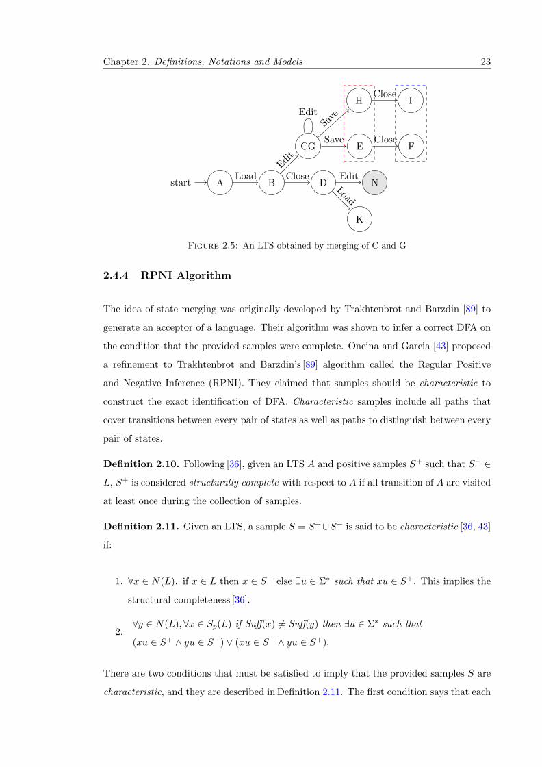
Chapter 2. Definitions, Notations and Models 23
Astart B
CG
D
E
H I
F
N
K
Load
Edit
Close
Save
EditSa
ve
Close
Close
Edit
Load
Figure 2.5: An LTS obtained by merging of C and G
2.4.4 RPNI Algorithm
The idea of state merging was originally developed by Trakhtenbrot and Barzdin [89] to
generate an acceptor of a language. Their algorithm was shown to infer a correct DFA on
the condition that the provided samples were complete. Oncina and Garcia [43] proposed
a refinement to Trakhtenbrot and Barzdin’s [89] algorithm called the Regular Positive
and Negative Inference (RPNI). They claimed that samples should be characteristic to
construct the exact identification of DFA. Characteristic samples include all paths that
cover transitions between every pair of states as well as paths to distinguish between every
pair of states.
Definition 2.10. Following [36], given an LTS A and positive samples S+ such that S+ ∈
L, S+ is considered structurally complete with respect to A if all transition of A are visited
at least once during the collection of samples.
Definition 2.11. Given an LTS, a sample S = S+∪S− is said to be characteristic [36, 43]
if:
1. ∀x ∈ N(L), if x ∈ L then x ∈ S+ else ∃u ∈ Σ∗ such that xu ∈ S+. This implies the
structural completeness [36].
2.∀y ∈ N(L), ∀x ∈ Sp(L) if Suff(x) 6= Suff(y) then ∃u ∈ Σ∗ such that
(xu ∈ S+ ∧ yu ∈ S−) ∨ (xu ∈ S− ∧ yu ∈ S+).
There are two conditions that must be satisfied to imply that the provided samples S are
characteristic, and they are described in Definition 2.11. The first condition says that each

Chapter 2. Definitions, Notations and Models 24
sequence x in the kernel N belongs to the correct language L, it also belongs to the set
of positive samples S+, otherwise the sequence x can be a prefix for other suffixes u in
which the sequence xu belongs to S+. The second condition implies that a suffix u would
distinguish states whenever a sequence x in the set of short prefixes Sp(L) and y belong
to the kernel N if they do not have the same set of suffixes Suff(x) 6= Suff(y).
Before we describe the RPNI algorithm, the following notation is used: supposeA=(Q,Σ, F, δ, q0)
is a finite state machine, and let π be a partition of states Q of A. A subset of elements
of a partition is called block B. Provided mergers of all states in each block are valid, a
quotient automaton A/π is obtained by merging states that belong to the same block of
π.
The whole body of the RPNI algorithm is provided in Algorithm 2. The RPNI takes a
finite set of positive and negative samples and constructs the corresponding PTA from
the positive samples. The negative samples are introduced to stop merging states if the
resulting automaton leads to accept negative samples. It performs a breadth-first search
to identify pairs of states to merge. After constructing the APTA from the positive and
negative samples, an initial partition π is determined. At each step of the generalization,
two blocks (Bi, Bj) of the partition π are selected for merging. During the merging of
blocks, a non-deterministic automaton might be obtained, and the partition is then up-
dated to solve the non-determinism. After merging them, a new intermediate hypothesis
automaton is obtained PTA/πnew. Once the new hypothesis solution is compatible with
the negative samples, the partition π is updated with πnew as shown in line 6, otherwise
the solution is rejected. The generalization process continues by selecting other candidates
of blocks to merge until no more states can be merged.
input : S+ and S−
/* Sets of accepted and rejected sequences */
result: A is a DFA that is compatible with S+ and S−
1 PTA← Initialize (S+)2 π ← {{0}, {1}, · · · {N − 1}}3 while (Bi, Bj)← SelectPairofBlocks (π) do4 πnew ← Merge (π,Bi, Bj)5 if Compatible (PTA/πnew, S
−) then6 π ← πnew7 end
8 end
Algorithm 2: RPNI algorithm [90]
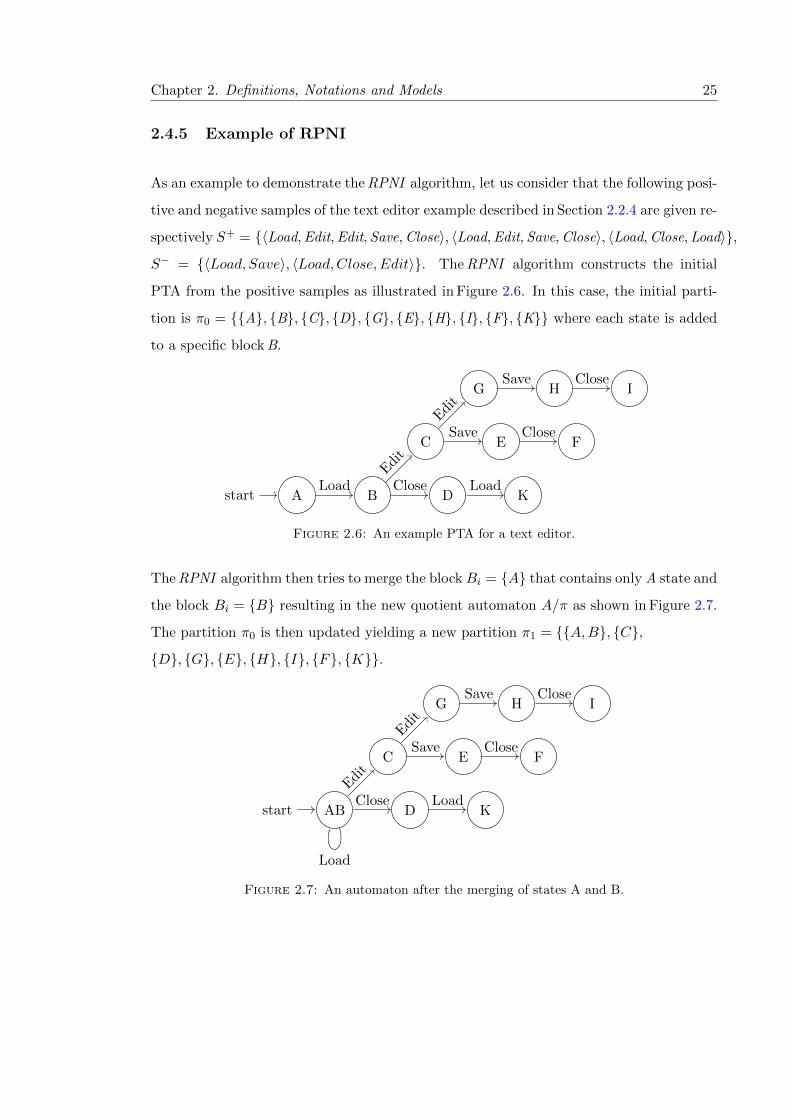
Chapter 2. Definitions, Notations and Models 25
2.4.5 Example of RPNI
As an example to demonstrate the RPNI algorithm, let us consider that the following posi-
tive and negative samples of the text editor example described in Section 2.2.4 are given re-
spectively S+ = {〈Load,Edit,Edit,Save,Close〉, 〈Load,Edit,Save,Close〉, 〈Load,Close,Load〉},
S− = {〈Load, Save〉, 〈Load,Close, Edit〉}. The RPNI algorithm constructs the initial
PTA from the positive samples as illustrated in Figure 2.6. In this case, the initial parti-
tion is π0 = {{A}, {B}, {C}, {D}, {G}, {E}, {H}, {I}, {F}, {K}} where each state is added
to a specific block B.
Astart B
C
D
G
E
H I
F
KLoad
Edit
Close
Edit
Save
Save Close
Close
Load
Figure 2.6: An example PTA for a text editor.
The RPNI algorithm then tries to merge the block Bi = {A} that contains only A state and
the block Bi = {B} resulting in the new quotient automaton A/π as shown in Figure 2.7.
The partition π0 is then updated yielding a new partition π1 = {{A,B}, {C},
{D}, {G}, {E}, {H}, {I}, {F}, {K}}.
ABstart
C
D
G
E
H I
F
K
Load
Edit
Close
Edit
Save
Save Close
Close
Load
Figure 2.7: An automaton after the merging of states A and B.

Chapter 2. Definitions, Notations and Models 26
2.5 Evaluation of Software Models
This section describes the methods of evaluating state-machine inference algorithms from
different points of view. It includes methods that rely on generating test sequences using
the W-method or random walks for evaluating the inferred models.
It is difficult to evaluate and compare state-machine inference techniques since there is no
standardized way to accomplish this. Pradel et al. [97] stated that the task of evaluating
different specification miners is difficult since there are no common methods to assess the
quality of mined specifications. In general, the common way is to evaluate and compare
the inferred state machines against their reference models. They are intended to represent
software being reverse engineered.
2.5.1 The W-method
The W-method is the most common method of generating tests from an automaton. It
and was originally proposed by Chow [91], Vasilevskii [92] for generating test cases from
FSMs. The W-method has been investigated to generate tests from different kinds of
state machines. For instance, Bogdanov et al. [93] used the W-method to construct test
sequences from X-machines models. Whereas, Ipate and Banica [94] adapted the W-
method to generate test sequences from hierarchical FSMs. Moreover, variations of the
W-method have been developed, for example, Fujiwara et al. [95] proposed the partial
W-method (Wp-method) to reduce the length of test sets.
To describe the W-method in the context of comparing two different LTSs, given a speci-
fication LTS S and an implementation LTS I, the aim of the W-method is to construct a
test set, which is a finite set of sequences (test cases), from S to measure the conformity
of I against S. The test set TS should cover each state of S in order to find contradictions
between I and S by passing TS as tests to I. Once the implementation I generates the
corresponding outputs to the test sequences TS, those outputs would be compared to the
correct ones of S.
The task of checking the conformance between an implementation LTS I and a specification
LTS S can be unsolved as I may contain extra faulty states that cannot be visited by the
generated test set [13]. In a testing context, it is difficult to know the maximum number

Chapter 2. Definitions, Notations and Models 27
of states m in the implementation I. Also, a tester may not have access to the correct
implementation [13, 91]. In this case, a tester has to estimate m. This phase is critical
where an incorrect estimation of m may cause the generation of inadequate test sets.
The W-method begins by estimating the number of states in the implementation I. Once
the maximum number of states m is known or estimated, the W-method makes some
assumptions about the specification S and the implementation I. The specification S
should be minimal, completely specified and deterministic. Such assumptions are necessary
in order to generate a finite set of test sets to ensure that the implementation I is correctly
implemented against the specification S. The W-method assumes that the number of states
m in I may be larger than the number of states n in S.
� Construction of state cover set C.
A state cover set C of a specification LTS S is a prefixed-closed set of sequences that
are required to visit each state of an LTS S from the initial state q0 ∈ Q at least
once.
Definition 2.12. C ⊆ Σ∗ is said to be a state cover of an LTS S such that C ⊂ L(S)
if ε ∈ C and ∀q ∈ Q\{q0}, ∃c ∈ C such that δ (q0, c) = q.
In the text editor example shown in Figure 2.1, the state cover set is S = {ε, 〈Load〉, 〈Exit〉,
〈Load, Edit〉}.
� Construction of characterization set W .
Definition 2.13. Given a set of input sequences W such that W ⊆ Σ∗ and two states
q1, q2 ∈ Q. So, q1, q2 is said W-distinguishable if (L(S, q1)∩W ) 6= (L(S, q2)∩W ) [13].
The set of input sequences that can distinguish between any two states in S is called
a characterization or separation set.
Definition 2.14. Given a set of input sequences W such that W ⊆ Σ∗. W is called a
characterization set [96] of S if any two distinct states of S are W-distinguishable [13].
In the text editor example shown in Figure 2.1, the W set isW = {〈Exit〉, 〈Save〉, 〈Close〉}.

Chapter 2. Definitions, Notations and Models 28
� Construction of transition cover set P .
In the traditional W-method, a transition cover set P for a specification LTS S is a
finite set which contains all the sequences of inputs that visits each transition in S.
Definition 2.15. A transition cover P is a prefixed-closed set containing all se-
quences of inputs needed to visit every transition of an LTS S from the initial state
q0. That is, for each state ∀q ∈ Q and for each element of an alphabet ∀a ∈ Σ there
exists a p ∈ P such that δ (q, p · a) = q1 for some q1 ∈ Q .
Walkinshaw and Bogdanov [13] defined P in terms of state cover set as follows:
P = (C ∪ CΣ) (2.1)
In the text editor example shown in Figure 2.1, the transition cover set is P =
{ε, 〈Exit〉, 〈Load〉, 〈Load, Edit〉, 〈Load, Close〉, 〈Load, Edit, Save〉, 〈Load, Edit, Edit〉,
〈Load, Edit, Close〉, 〈Load, Edit, Exit〉}.
� Construction of distinguishing set Z.
Z = ({ε} ∪ Σ · · ·Σm−n)W (2.2)
In the text editor example shown in Figure 2.1, the Z Set is Z = {〈Exit〉, 〈Save〉,
〈Close〉, 〈Load, Exit〉, 〈Load, Save〉, 〈Load, Close〉, 〈Exit, Exit〉, 〈Exit, Save〉, 〈Exit,Close〉,
〈Close, Exit〉, 〈Close, Save〉, 〈Close, Close〉, 〈Edit, Exit〉, 〈Edit,Save〉, 〈Edit, Close〉,
〈Save, Exit〉, 〈Save, Save〉, 〈Save, Close〉}.
� Construction of test set TS.
The test set TS is obtained by computing the cross product of two sets P and Z:
TS = P × Z (2.3)
TS = (C ∪ CΣ)({ε} ∪ Σ · · ·Σm−n)W (2.4)

Chapter 2. Definitions, Notations and Models 29
TS = C({ε} ∪ Σ)({ε} ∪ Σ · · ·Σm−n)W (2.5)
TS = C({ε} ∪ Σ · · ·Σm−n+1)W (2.6)
In the text editor example shown in Figure 2.1, the test set is TS = {〈Close〉, 〈Edit〉,
〈Save〉, 〈Exit, Edit〉, 〈Exit, Load〉, 〈Exit, Close〉, 〈Exit, Save〉, 〈Exit, Exit〉, 〈Load, Load〉,
〈Load, Save〉, 〈Load, Close, Edit〉, 〈Load, Close, Close〉, 〈Load, Close, Save〉,
〈Load, Exit, Edit〉, 〈Load, Exit, Load〉, 〈Load, Exit, Close〉, 〈Load, Exit, Save〉,
〈Load, Exit, Exit〉, 〈Load, Edit, Load〉, 〈Load, Edit, Exit, Exit〉, 〈Load, Edit, Exit, Save〉,
〈Load, Edit, Exit, Close〉, 〈Load, Edit, Exit, Load〉, 〈Load, Edit, Exit, Edit〉,
〈Load, Edit, Save, Save〉, 〈Load, Edit, Save, Load〉, 〈Load, Edit, Close, Save〉,
〈Load, Edit, Close, Close〉, 〈Load, Edit, Close, Edit〉, 〈Load, Edit, Edit, Load〉,
〈Load, Close, Exit, Exit〉, 〈Load, Close, Exit, Save〉, 〈Load, Close, Exit, Close〉,
〈Load, Close, Load, Exit〉, 〈Load, Close, Load, Save〉, 〈Load, Close, Load, Close〉,
〈Load, Edit, Save, Exit, Exit〉, 〈Load, Edit, Save, Exit, Save〉,
〈Load, Edit, Save, Exit, Close〉, 〈Load, Edit, Save, Close, Exit〉,
〈Load, Edit, Save, Close, Save〉, 〈Load, Edit, Save, Close, Close〉,
〈Load, Edit, Save, Edit, Exit〉, 〈Load, Edit, Save, Edit, Save〉,
〈Load, Edit, Save, Edit, Close〉, 〈Load, Edit, Close, Exit, Exit〉,
〈Load, Edit, Close, Exit, Save〉, 〈Load, Edit, Close, Exit, Close〉,
〈Load, Edit, Close, Load, Exit〉, 〈Load, Edit, Close, Load, Save〉,
〈Load, Edit, Close, Load, Close〉, 〈Load, Edit, Edit, Exit, Exit〉,
〈Load, Edit, Edit, Exit, Save〉, 〈Load, Edit, Edit, Exit, Close〉,
〈Load, Edit, Edit, Save, Exit〉, 〈Load, Edit, Edit, Save, Save〉,
〈Load, Edit, Edit, Save, Close〉, 〈Load, Edit, Edit, Close, Exit〉,
〈Load, Edit, Edit, Close, Save〉, 〈Load, Edit, Edit, Close, Close〉,
〈Load, Edit, Edit, Edit, Exit〉, 〈Load, Edit, Edit, Edit, Save〉,
〈Load, Edit, Edit, Edit, Close〉}.
Chapter 2. Definitions, Notations and Models 30
2.5.2 Comparing Two Models in Terms of Language
In the grammar inference domain, the process of evaluating the inferred models was
originally proposed by Lang et al. [44] for the Abbadingo-One competition. The pro-
cess involves generating random samples as test sequences for evaluation purposes, and
then the number of test sequences that are correctly classified by the inferred model are
counted [44]. Walkinshaw and Bogdanov [13] stated that the set of random tests needs to
be diverse, where half of the samples belong to the language of the reference model, and
the other half do not.
Walkinshaw and Bogdanov [13] claimed that the approach of taking random samples of
test sequences that was applied by Lang et al. [44] causes two problems. The first issue
is that obtaining randomly representative test sequences is impossible. This is because
they will be biased towards some paths that are easily reached whenever sequences are
generated randomly from the transition structure of a state machine [13]. The second
problem relates to the metric that is used by Lang et al. [44] to compute the number of
sequences that are classified correctly by both models (the inferred and reference LTSs or
machines). This metric does not specify qualitative perceptions about differences between
two models in terms of their languages [13]. For example, a low value of the metric such
as 50% does not determine whether the inferred model tends to accept all sequences, or it
equally correctly classifies [13].
On the other hand, Lo and Khoo [98] presented a Quality Assurance Framework (QUARK)
to assess a specification inference. In QUARK [98], different dimensions were introduced
to be considered for evaluating the quality of specification miners. The first factor is
the scalability of a specification miner that measures its ability to infer accurately larger
models. The accuracy also needs to be taken into account to measure the extent to which
the specification inference can infer a model that is representative of the actual correct
specification. In our context, the inferred models are said accurate if it is representative
of the software being inferred. The robustness concerns the sensitivity of an inference
algorithm to errors in training data. A specification miner is considered good among other
miners if it can infer a very accurate specification compared to the reference specification
on the condition that training data is characteristic [98].

Chapter 2. Definitions, Notations and Models 31
In the QUARK framework [98], a specification miner and a simulator automaton that is
defined by the user (reference model) are first given to QUARK. In addition, the percentage
of the errors in the simulator is identified in order to examine the robustness of the miner.
The QUARK framework then generates different sets of traces, each trace is a sequence of
method calls, from the simulator model including erroneous traces. Those sets are fed into
the specification miner to infer an automaton. It compares the behaviour of the inferred
automaton against that of the reference model.
In the QUARK framework, Lo and Khoo [98] suggested generating two sets of traces for
measuring the accuracy of a specification miner: the first set is obtained from the given
reference model R and the second set is generated from the inferred model I. Lo and
Khoo [98] proposed two metrics to evaluate the similarities between R and I. The metrics
are computed based on the two generated sets of traces. The first metric measures the
proportion of traces that are generated by R and accepted by I. This metric represents
the ratio of correctly inferred information by the mined model [98]. In the information
retrieval community, this metric is also known as recall [99]. The second measurement
computes the percentage of sequences that are generated by I, and accepted by R [98].
This summarizes the quantity of correctly produced information by I. The second metric
is also known as precision in the information retrieval domain [99]. In this chapter, we
denote this manner of computing the precision and recall metrics as the conventional
precision-recall.
Walkinshaw et al. [100] illustrated the conventional approach of computing precision-recall
that is used in the QUARK framework [98] and explored the related issues. The compu-
tation of the conventional precision-recall is achieved by generating random samples from
the target and inferred models to find the overlap between them. The random sequences
are classified into retrieved (RET ) and relevant (REL) sets depending on what is retrieved
and relevant as illustrated in Table 2.1. If a sequence e is classified as accepted for both
machines such that e ∈ L(R)∧e ∈ L(I), then e is added to both RET and REL sets. If the
sample e is classified only as accepted by the inferred model such that e /∈ L(R)∧e ∈ L(I),
then e is only added to the RET set, and so on. The precision and recall are then com-
puted based on RET and REL sets after classifying each sequence in the test set. The
precision and recall are computed as follows:

Chapter 2. Definitions, Notations and Models 32
Precision =|REL ∩RET ||RET |
(2.7)
Recall =|REL ∩RET ||REL|
(2.8)
I Machine (Inferred) R Machine (Reference) RET REL
accept accept√ √
accept reject√
reject accept√
reject reject
Table 2.1: Conventional manner of classifying sequences into relevant and retrieved sets
Walkinshaw et al. [100] claimed that the use of precision and recall measurements in the
conventional method as described (above) by Lo and Khoo [98] to evaluate the accuracy
of the mined models can be problematic. The conventional method has two shortcomings.
First, random-positive test sets that are generated to detect the differences between the
mined and reference models may ignore some sequences that are less likely to be generated.
It only covers the disagreement between the models based on sequences that are easy
to reach when they are randomly generated [100]. Hence, computing precision and recall
based on such test sets will result in unreliable scores. Second, the computation of precision
and recall in the conventional way is biased towards accepting sequences (behaviours) of the
mined and reference models [100]. Therefore, it is important to include invalid sequences.
However, even if they are included in the conventional manner, it will not make sense
because the precision and recall rely on positive samples only. For instance, if a sequence
e is rejected by both models, the RET and REL sets do not count for this case as shown
in the last row in Table 2.1.
Walkinshaw et al. [100] addressed this first problem by applying the idea of conformance
testing methods in order to obtain positive and negative sequences. They [100] suggested
using techniques such as the W-method to generate a test set, which contains valid and
invalid sequences that are not biased towards accepting behaviours of the reference ma-
chine. However, the test set tends to be very large making the execution of the whole
test set unfeasible, since it is highly costly in practice [100]. Nevertheless, the balance that
is required between positive and negative test sequences in the test set will be missed;
this is because the vast majority of sequences that can be generated using W-method are

Chapter 2. Definitions, Notations and Models 33
rejected [13]. This would lead a high score to the inferred state machine that rejects all
sequences because it does not count for the balance assessment for the accuracy of the
inferred state machines [35, 100].
Instead of applying Lo and Khoo’s [98] idea of generating random samples from both the
mined and target machines, Walkinshaw et al. [100] proposed using the concept of model-
based testing approaches in which a test set is generated from the target machine. This
would highlight the disagreement between the grammars of the inferred and target state-
machine models. Walkinshaw et al. [100] refined the conventional precision-recall in order
to use them for classifying accepting and rejecting sequences. It is suggested to compute
a specific precision for positive sequences and another one for negative ones. Additionally,
they also [100] compute the recall for both categories (negatives and positives) of sequences.
To achieve this, instead of categorizing test sequences into RET and REL sets, Walkinshaw
et al. [100] divided both sets into RET+ RET−, REL+, and REL− sub-sets. Thus, test
sequences are added to those sub-sets as shown in Table 2.2. The refined precision and
recall metrics are shown in Table 2.3
I Machine (Inferred) R Machine (Reference) RET+ REL+ RET− REL−
accept accept√ √
accept reject√ √
reject accept√ √
reject reject√ √
Table 2.2: Refined-way of classifying sequences into relevant and retrieved sets
Precision+ = |REL+∩RET+||RET+| Precision− = |REL−∩RET−|
|RET−|
Recall+ = |REL+∩RET+||REL+| Recall− = |REL−∩RET−|
|REL−|
Table 2.3: Refined-way of computing the precision and recall
A high value of Precision+ indicates that the majority of the returned positive sequences
are correctly represented (classified) by the inferred (mined) as positive with respect to
the reference model (correctness). Moreover, a high value of Recall+ indicates that a
large number of relevant accepted test sequences are correctly retrieved by the inferred
(hypothesis) model (completeness); and vice versa for Precision− and Recall−.
Walkinshaw and Bogdanov [13] showed how to compare the similarities between two LTSs
in terms of the language. To achieve this, test sequences are generated using the W-method
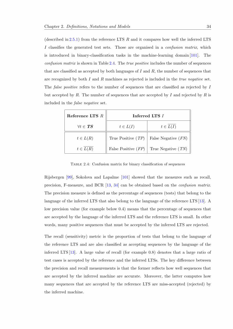
Chapter 2. Definitions, Notations and Models 34
(described in 2.5.1) from the reference LTS R and it compares how well the inferred LTS
I classifies the generated test sets. Those are organised in a confusion matrix, which
is introduced in binary-classification tasks in the machine-learning domain [101]. The
confusion matrix is shown in Table 2.4. The true positive includes the number of sequences
that are classified as accepted by both languages of I and R, the number of sequences that
are recognized by both I and R machines as rejected is included in the true negative set.
The false positive refers to the number of sequences that are classified as rejected by I
but accepted by R. The number of sequences that are accepted by I and rejected by R is
included in the false negative set.
Reference LTS R Inferred LTS I
∀t ∈ TS t ∈ L(I) t ∈ L(I)
t ∈ L(R) True Positive (TP) False Negative (FN)
t ∈ L(R) False Positive (FP) True Negative (TN)
Table 2.4: Confusion matrix for binary classification of sequences
Rijsbergen [99], Sokolova and Lapalme [101] showed that the measures such as recall,
precision, F-measure, and BCR [13, 34] can be obtained based on the confusion matrix.
The precision measure is defined as the percentage of sequences (tests) that belong to the
language of the inferred LTS that also belong to the language of the reference LTS [13]. A
low precision value (for example below 0.4) means that the percentage of sequences that
are accepted by the language of the inferred LTS and the reference LTS is small. In other
words, many positive sequences that must be accepted by the inferred LTS are rejected.
The recall (sensitivity) metric is the proportion of tests that belong to the language of
the reference LTS and are also classified as accepting sequences by the language of the
inferred LTS [13]. A large value of recall (for example 0.8) denotes that a large ratio of
test cases is accepted by the reference and the inferred LTSs. The key difference between
the precision and recall measurements is that the former reflects how well sequences that
are accepted by the inferred machine are accurate. Moreover, the latter computes how
many sequences that are accepted by the reference LTS are miss-accepted (rejected) by
the inferred machine.
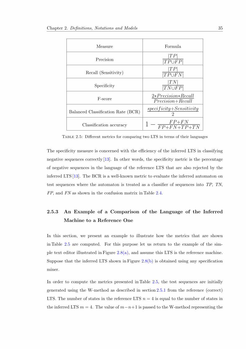
Chapter 2. Definitions, Notations and Models 35
Measure Formula
Precision|TP |
|TP∪FP |
Recall (Sensitivity)|TP |
|TP∪FN |
Specificity|TN |
|TN∪FP |
F-score2∗Precision∗RecallPrecision+Recall
Balanced Classification Rate (BCR)specificity+Sensitivity
2
Classification accuracy 1− FP+FNFP+FN+TP+TN
Table 2.5: Different metrics for comparing two LTS in terms of their languages
The specificity measure is concerned with the efficiency of the inferred LTS in classifying
negative sequences correctly [13]. In other words, the specificity metric is the percentage
of negative sequences in the language of the reference LTS that are also rejected by the
inferred LTS [13]. The BCR is a well-known metric to evaluate the inferred automaton on
test sequences where the automaton is treated as a classifier of sequences into TP, TN,
FP, and FN as shown in the confusion matrix in Table 2.4.
2.5.3 An Example of a Comparison of the Language of the Inferred
Machine to a Reference One
In this section, we present an example to illustrate how the metrics that are shown
in Table 2.5 are computed. For this purpose let us return to the example of the sim-
ple text editor illustrated in Figure 2.8(a), and assume this LTS is the reference machine.
Suppose that the inferred LTS shown in Figure 2.8(b) is obtained using any specification
miner.
In order to compute the metrics presented in Table 2.5, the test sequences are initially
generated using the W-method as described in section 2.5.1 from the reference (correct)
LTS. The number of states in the reference LTS n = 4 is equal to the number of states in
the inferred LTS m = 4. The value of m−n+1 is passed to the W-method representing the

Chapter 2. Definitions, Notations and Models 36
Astart B D
E
LoadExit
Exit
Close
Edit
Edit
Close
Save
Exit
(a) The reference LTS of a text editor
Astart B D
E
Load
Exit
Close
Edit
Save
Edit
(b) The inferred LTS of a text editor
Figure 2.8: The reference LTS and the mined one of the text editor example
number of extra states in the inferred LTS. The number of tests generated using the W-
method is 63. Table A.1 that is shown in appendix A provides the tests that are generated
using the W-method and their classifications by both the reference and inferred LTSs.
Reference LTS R Inferred LTS I
∀t ∈ TS t ∈ L(I) t ∈ L(I)
t ∈ L(R) TP = 2 FN = 12
t ∈ L(R) FP = 0 TN = 49
Table 2.6: Confusion matrix for binary classification of sequences
The confusion matrix is built from the classification of the test sets as shown in Table 2.6.
The outcomes of computing different metrics are presented in Table 2.7. The high score of
precision means that all sequences that are classified by the inferred LTS as positive are also
classified as positive by the reference LTS. On the other hand, the low value of recall (0.14)
indicates that the inferred LTS rejects (classified as negative) a large number of sequences
that must be accepted (classified as positive) according to the language of the reference
LTS. This is because twelve out of fourteen positive-sequences are classified by the inferred
LTS as negatives. The F-measure score (0.25) tells us the harmonic mean that combines

Chapter 2. Definitions, Notations and Models 37
the precision and recall measures and indicates that the inferred automaton incorrectly
classifies positive test sequences. The F-measure does not account for the accuracy of
the inferred automaton in terms of its language complements. The BCR score of 0.57 is
obtained by computing the average of recall and specificity which tells us the accuracy of
the inferred automaton at classifying positive and negative.
Measure Score
Precision 1.0
Recall (Sensitivity) 0.14
Specificity 1.0
F-score 0.25
Balanced Classification Rate (BCR) 0.57
Table 2.7: Metrics scores obtained from confusion matrix
2.5.4 Comparing Two Models in Terms of Structure
It is important to consider the structure of the inferred models when a software engineer
compares them to their target models. Walkinshaw and Bogdanov [13] stated that the
comparison of two state machines in terms of their structures can provide complementary
insights into the dissimilarity of two state machines that cannot be obtained by comparing
their languages. However, comparing two different LTSs in terms of structure is not
necessary an easy task [51].
Walkinshaw and Bogdanov [13] proposed the LTSDiff algorithm to accomplish the idea of
comparing two LTSs in term of their structures. The idea of comparing the inferred LTS
I and the reference LTS R revolves around determining which states and transitions are
deemed to be equivalent in both LTSs, and then finding states and transitions in the I
that are considered as extra or missing in comparison to R [13].
Chapter 2. Definitions, Notations and Models 38
2.5.4.1 LTSDiff Algorithm
Walkinshaw and Bogdanov [13] presented the LTSDiff algorithm to capture the differ-
ence between two state machine models, especially LTSs in terms of their structure. In
the LTSDiff algorithm, the comparison of two LTSs is established by measuring the simi-
larity scores of pairs of states with respect to the surrounding states and transitions. The
similarity score for a pair of states encodes the overlap of the surrounding states and tran-
sitions. Moreover, it can be computed locally based on the immediate transitions of two
states, and globally based on the target and source states of those transitions.
The LTSDiff algorithm begins by the given two automata I,R. R denotes the reference
LTS and I denotes the inferred LTS. It aims with a high level of confidence to identify
pairs of states (s1, s2) such that s1 ∈ QI ∧ s2 ∈ QR that are most likely be equivalent.
Those pairs are called key pairs and considered as common landmarks that exist in both
automata. The dissimilarity between I,R can be detecting based on landmarks, where
states and transition comparisons in both automata rely on landmarks [13, 51].
In general, the idea of comparing two LTS in terms of their structures used in the LTSDiff
algorithm can be seen as a human pointing to an unknown landscape in a map and
looking for an identifiable place (landmark) near to the landscape and attempting to
locate it on the map [13]. In the LTSDiff algorithm, easily recognizable states are those
that are surrounded by distinctive states and transitions; such identifiable states are used
as landmarks for further comparison. The LTSDiff algorithm is provided in Algorithm 3
and is summarized in the following phases:
First Identifying Key Pairs. In the LTSDiff algorithm, this is denoted by computeScores.
The LTSDiff algorithm identifies the key pairs by computing the similarity scores
(described later in this section) for any given pair of states (A,C) in terms of its
transitions. The pairs of states that have the highest similarity score are selected
to be reference points and are considered as key pairs. The computation of the
structural differences between two LTSs starts from the reference point, and then
compares the surrounding pairs of states and transitions until no further comparison
can be found.

Chapter 2. Definitions, Notations and Models 39
� Local similarity score
Essentially, the similarity (matching) score of the pair of states (A,C) is ob-
tained by computing the average of common transitions between two states.
This is called a local similarity score. As we are interesting in a deterministic
machine, the similarity score is computed by SAC =Σ(A) ∩ Σ(C)
Σ(A) ∪ Σ(C). Table 2.8
shows four examples for computing the similarity score of two deterministic
states (A,C). In Figure(a) in Table 2.8, outgoing transitions of the states (A,C)
share the same Load label and this yields a score of 1. In Figure(b), there is no
outgoing transitions with same labels, which makes the similarity score zero.
A B
C D
Load
Load
Sac =1
1= 1
A B
C D
Load
Edit
Sac =0
2= 0
(a) (b)
A B
C D
E
Load
Load
Edit
Sac =1
2= 0.5
A B
C D
E
F
LoadClose
Load
Edit
Sac =1
3= 0.3
(c) (d)
Table 2.8: Example of the similarity score computation
The computation of the local similarity score is defined and re-written [13] to
count for non-deterministic state machine. The equation of computing the local
similarity score is shown in Equation 2.9 for the given two states (A,C) such
that A ∈ QI , C ∈ QR.
SLSucc(A,C) [13] =| SuccA,C |
| ΣoutI (A)− Σout
R (C) | + | ΣoutI (C)− Σout
R (A) | + | SuccA,C |(2.9)

Chapter 2. Definitions, Notations and Models 40
In Equation 2.9, two states are given (A,C) such that A ∈ QI , C ∈ QR. The
| SuccA,C | denotes to the set of target states pairs that can be reached using
the common transitions for each possible label σ ∈ (ΣI ∪ΣR). Definition 2.16 is
defined formally in [13].
Definition 2.16. Following [13] Let B ∈ QI , D ∈ QR, and σ ∈ (ΣI ∪ ΣR)
SuccA,C = {(B,D, σ) | δ(A, σ) = B ∧ δ(C, σ) = D}
The notation ΣoutI (A) in Equation 2.9 denotes the labels of outgoing transi-
tions (alphabets) from state A of LTS I. Therefore, the expression | ΣoutI (A)−
ΣoutR (C) | returns the number of elements of an alphabet corresponding un-
matched outgoing transitions from state A compared to that from state C, and
vice versa for the expression | ΣoutI (C)− Σout
R (A) |.
For example, in Figure(C) in Table 2.8, the number of unmatched outgoing
transitions between the state C compared to the state A is one (written as
| ΣoutI (C)−Σout
R (A) |= 1 ). In this example, the expression | ΣoutI (A)−Σout
R (C) |
returns zero because only one outgoing transition from state A, which is Load, is
matched with the outgoing transitions from state C. In addition, the expression
| ΣoutI (C)−Σout
R (A) | returns one because the outgoing transition from state C
that is labelled with Edit does not match with any other outgoing transitions
from state A. So, SLSucc(A,C) =1
0 + 1 + 1= 0.5.
The equation 2.9 is concerned with computing the local similarity with re-
spect to pairs of states that share the outgoing transitions. Walkinshaw and
Bogdanov [13] defined the local similarity for incoming transitions as shown
formally in Definition 2.10.
SLPrev(A,C) [13] =| PrevA,C |
| ΣincI (A)− Σinc
R (C) | + | ΣincI (C)− Σinc
R (A) | + | PrevA,C |(2.10)
Following [13], the set of matching transition for a given states (A,C).
Definition 2.17. Following [13] Let B ∈ QI , D ∈ QR, and σ ∈ (ΣI ∪ ΣR)
PrevA,C = {(B,D, σ) | δ(B, σ) = A ∧ δ(D,σ) = C}

Chapter 2. Definitions, Notations and Models 41
The notation ΣincI (A) denotes the incoming transitions to state A. Other expres-
sions are defined in equation Equation 2.10 in the same way as in Equation 2.9.
� Global similarity score
The above computations of local similarity scores that are shown in equa-
tions 2.9 and 2.10 focus on measuring the similarity of states based on the neigh-
bouring transitions. To this regard it is necessary to also consider the wider
context. Walkinshaw and Bogdanov [13] showed the global similarity score that
intends to measure the transition similarity for source and target states of ad-
jacent transitions as well.
The computation of global similarity aimed to assign a higher score if the source
and target states of the matched transitions are similar, and a lower score if
they are different [13]. The computation procedure of the global similarity score
SG1Succ(A,C) extends the local similarity score SLSucc(A,C) that is illustrated in
equation 2.9. The following equation computes recursively the similarity for the
target states of a pair of states, and this is not considered in the local similarity
score.
SG1Succ(A,C) =
1
2
Σ(B,D,σ)∈SuccA,C(1 + SG1
Succ(B,D))
| ΣoutI (A)− Σout
R (C) | + | ΣoutI (C)− Σout
R (A) | + | SuccA,C |(2.11)
Walkinshaw and Bogdanov [13] stated that the procedure of computing the
global similarity score that is introduced in equation 2.11 can lead to unintu-
itive scores. This is because for any given pair of states (A,C), the recursive
computation of the score can count for sequential target pairs of states that are
not closer to (A,C). To give priority to pairs of states that are closer to the
pair of interest, Walkinshaw and Bogdanov [13] introduced an attenuation ratio
K as shown in the following equation 2.12.
SGSucc(A,C) [13] =1
2
Σ(B,D,σ)∈SuccA,C(1 + kSGSucc(B,D))
| ΣoutI (A)− Σout
R (C) | + | ΣoutI (C)− Σout
R (A) | + | SuccA,C |(2.12)

Chapter 2. Definitions, Notations and Models 42
In the same way, Walkinshaw and Bogdanov [13] defined SGPrev(A,C) to com-
pute the global similarity score in terms of the incoming transitions as follows:
SGPrev(A,C) [13] =1
2
Σ(B,D,σ)∈PrevA,C(1 + kSGPrev(B,D))
| ΣincI (A)− Σinc
R (C) | + | ΣincI (C)− Σinc
R (A) | + | PrevA,C |(2.13)
The final global score for each pair of states is computed in terms of incoming
and outgoing transitions by taking the average of two notations SGSucc(A,C)
and SGPrev(A,C) as follows:
S(A,C) [13] =SGSucc(A,C) + SGPrev(A,C)
2(2.14)
The above computation of scores is denoted by the computeScores (LTSI , LTSR, k)
function in the LTSDiff Algorithm 3.
Once the scores of state pairs are computed, the LTSDiff algorithm selects state
pairs that have the greatest possibility to be equivalent in the two-stage approach
as follows:
1. Introduce a threshold parameter t where pairs of states with scores above t are
considered for the process of identifying key pairs. Walkinshaw and Bogdanov
[13] stated that a state may be matched to multiple states, although this am-
biguity is not preferable.
2. To reduce the ambiguities made in the previous step, Walkinshaw and Bogdanov
[13] suggested selecting only one pair of states to be a key pair if its score
is better than any other pairs beyond any doubt. In this case, a ratio r is
introduced as a second criterion to select only pairs that are suggested to be
the best match r times compared to other matches. Thus, the best matched
pairs are added to the key pairs.
In the LTSDiff algorithm shown in Algorithm 3, the above strategy of selecting the
best pairs of states is denoted by identifyLandmarks that is working as a filtering
process by passing the set of pairs, the threshold t, and r to collect the key pairs.
The LTSDiff algorithm then collects the set of matched state pairs (NPairs) that
surround each key pair. The surrounding pairs of states for a given pair (A,C)
are defined as follows: SurrA,C = {(B,D) ∈ QI × QR | ∃σ ∈ (ΣI ∪ ΣR)·((A
σ→

Chapter 2. Definitions, Notations and Models 43
B ∧C σ→ D)∨ (Bσ→ A∧D σ→ C)
)}. The computation of SurrA,C is shown in line 6
in Algorithm 3 and the matched surrounding pairs of states are added to the NPairs
set
The procedure in the loop in the lines 7-14 in Algorithm 3 focuses on selecting the
matching pairs from the set of NPairs. It selects the pairs with the highest score
from the set of NPairs using pickHighest function. Once the pair with the highest
similarity has been selected, it is added to the list of KPairs.
Second Computing a Patch. Once the KPairs have been computed in lines 1-14, those
pairs of states are used to collect the differences between the two I,R LTSs; this
is referred to as a patch. For an inferred LTS I, the patch contains two sets of
transitions: The Removed set contains transitions that are removed from LTS I and
the Added set contains those transitions that are added to LTS I with comparison
with reference LTS R .
The computed patched can be used to compute the structural-similarity score. To illustrate
how the computed patch can be used to measure the structural difference between the
reference LTS R and the inferred LTS I in this thesis, Redge is used to denote the number of
edges in R, and Iedge refers to the number of edges in I. Removededges denotes the number
of edges that are missing from I, while Addededges means the number of edges that are
extra to I. The metric structural similarity is defined as an average of two measurements
(A,B), where the former computes how many transitions have not been inferred by a
learner that generated I, and the latter computes how many transitions of I that are
new to I. The pair (A,B) is computed using the equations 2.15, 2.16 respectively, and
the structural-similairty score is computed as shown in equation 2.17 .
A =Redge−Removededges
Redge(2.15)
B =Iedge−Addededges
Iedge(2.16)
structural-similarity score =A+B
2 (2.17)

Chapter 2. Definitions, Notations and Models 44
input : LTSI , LTSR, k, t, and r/* LTSs are the two machines, k is the attenuation value, t is the
threshold parameter, and r is the ratio of the best match to the
second-best score */
data : KPairs, PairsToScores,NPairsresult: Added,Removed,Renamed/* two sets of transitions and a relabelling */
1 PairsToScores← computeScores (LTSI , LTSR, k);2 KPairs← identifyLandmarks (PairsToScores, t, r);3 if KPairs = ∅ and S (p0, q0) then4 KPairs← (p0, q0);
/* p0 is the initial state in LTSI, q0 is the initial state in
LTSR */
5 end6 NPairs←
⋃a,b∈KPairs Surr (a, b)−KPairs;
7 while NPairs 6= ∅ do8 while NPairs 6= ∅ do9 (a, b)← pickHighest (NPairs,PairsToScores);
10 KPairs← KPairs ∪ (a, b);11 NPairs← removeConflicts (NPairs, (a, b));
12 end13 NPairs←
⋃a,b∈KPairs Surr (a, b)−KPairs;
14 end
15 Added← {b1σ→ b2 ∈ δR | @(a1
σ→ a2 ∈ δI ∧ (a1, b1) ∈ KPairs ∧ (a2, b2) ∈ KPairs)};16 Removed← {a1
σ→ a2 ∈ δI | @(b1σ→ b2 ∈ δR∧(a1, b1) ∈ KPairs∧(a2, b2) ∈ KPairs)};
17 Renamed← KPairs;18 return (Added,Removed,Renamed);
Algorithm 3: The LTSDiff Algorithm [13]
Example 2.1. For instance, consider the reference LTS of the text editor example shown
in Figure 2.9(a), and the inferred models of the text editor as depicted in Figure 2.9(b).
The output of the comparison using LTSDiff is given in Figure 2.10 where dashed (green)
transitions are missing and solid (red) transitions are incorrectly added to the inferred
model. A =9−2
9 = 0.778, and B =10−3
10 = 0.7. So, structural similarity is computed
using the equation 2.17.

Chapter 2. Definitions, Notations and Models 45
Astart B D
E
LoadExit
Exit
Close
Edit
Edit
Close
Save
Exit
(a) The reference LTS of a text editor
Astart B D
E
CLoad
Exit
Exit
Close
Edit
Close
Save
Edit
Exit
Close
(b) The inferred LTS of a text editor
Figure 2.9: Comparing the reference LTS and the mined one of the text editor exampleusing the LTSDiff Algorithm
Astart B D
E
CLoad
Exit
Exit
Close
Edit
Close
Save
Edit
Edit
Exit
Exit
Close
Figure 2.10: The output of LTSDiff between the reference LTS 2.9(a) and the inferredLTS 2.9(b) of a text editor example

Chapter 2. Definitions, Notations and Models 46
2.6 The Evaluation Technique in the Statechum Framework
In this section, the evaluation technique that will be used throughout the thesis is ex-
plained. Figure 2.11 demonstrates the general overview of the evaluation processes of the
inferred models in Statechum. It consists of four main phases. The first phase is called a
reference model generator, which is responsible for the generation of a reference LTS either
randomly generated LTSs or a real-world case studies LTSs. This phase is flexible because
it allows an analyst to manually provide their own reference or a real-world case studies
LTSs in different formats such as XML, which represents the states and transitions using
XML elements.
In the Statechum framework, the Forest Fire algorithm [102] is used to generate directed
random LTSs. The algorithm was developed by Walkinshaw and Bogdanov [13] to generate
random LTSs for the STAMINA competition [35]. A random LTS must be deterministic,
minimal, and every state must be reachable from the initial state.
Leskovec et al. [102] proposed the Forest-Fire algorithm to generate directed graphs that
represent complex networks. It is an iterative process that aims to add new nodes that
are connected to the other closest nodes in the graph. The Forest-Fire algorithm [102]
initially defines three parameters: the number of nodes (vertices) n, a backwards-burning
probability b, forward-burning ratio f , and self-looping probability s.
In the Forest-Fire model [102], nodes attach to a graph G at a time t and form outgoing
edges to the earlier nodes. Given the graph G, and considering that a node v arrives at a
time t to be attached to G. The current node v creates an outgoing arc to different nodes
in the graph G at a time t as follows: First, v chooses uniformly a random ambassador
node w where w 6= v, and create an edge from v to w. Second, two random numbers x and
y are generated and geometrically distributed such that x = f/(1−f) and y = fb/(1−fb).
Third, node v chooses outgoing and in-coming edges of node w to the non-visiting nodes
in the graph. Finally, node v generates outgoing edges to the target nodes of the selected
edges from and to node w, and repeats the second and third processes.
In this thesis, the Forest-Fire algorithm is used to generate random graphs with the fol-
lowing configurations: f = 0.31, b = 0.385 and s = 0.2. Those configurations were used
in [13] for the generation of random LTSs.

Chapter 2. Definitions, Notations and Models 47
Figure 2.11: The evaluation framework in Statechum
The second phase in the evaluation framework is the trace generator. Once a random
reference LTS is automatically generated, the training data are produced using random
walks from the target (reference) automata. The developer defines a number of parameters
as follows: the number of traces T and the length of the traces l.
Once the traces are generated from the reference automaton, one or more inference algo-
rithms takes those traces as inputs to learn automata using different state-merging strate-
gies. The synthesised LTS can be visualised for the analyst (software engineer). This is
the third phase in the evaluation process. Finally, the mined LTSs are used to compute
the variety of metrics such as precision, recall, F-measure, BCR. It also includes a compu-
tation of the structural similarity metric that is discussed in the LTSDiff 2.5.4.1 section.
In addition, statistical tests such as the Wilcoxon signed-rank test can be computed for
the metrics.

Chapter 2. Definitions, Notations and Models 48
2.7 DFA Inference Competitions
As mentioned earlier in this chapter, the task of evaluating the performance of state ma-
chines inference algorithms is a difficult task. Therefore, it is important to provide a
practical and scientific basis for comparing different techniques of inferring DFA models.
For this reason, researchers have organized a variety of competitions to compare and eval-
uate different inference techniques on the same DFA models. The following sub-sections
provide insights into different competitions for the comparison of inference techniques in
terms of their performance and capabilities to solve the different inference problems.
2.7.1 Abbadingo-One Competition
In the domain of grammar inference, numerous competitions were organised to allow com-
petitors to evaluate their DFA inference algorithms. In general, organisers generated a
set of random target models as problems to be solved by the competitors participating in
the competition. The competitors were only provided with training data to start learning
DFA. Sets of training samples were used for learning state-machine models and different
sets of tests were used to evaluate the performance of the inferred models. Lang et al.
[44] presented the first competition, which was named Abbadingo-One competition. The
competition was organised by Kevin J. Lang and Barak A. Pearlmutter. They posted
sixteen randomly generated DFAs as challenge problems.
The alphabet size used in Abbadingo-One competition was only two Σ = {0, 1}, implying
that the maximum number of transitions for each state was two. The process of generating
target DFAs of n size in this competition by construction of a directed graph of5
4n nodes.
The depth of the generated target machines was 2 log2 n− 2. The set of training data for
a target DFA of size n was randomly drawn from a uniform distribution over 16n2 − 1
strings and their length was between 0 and 2 log2 n+ 3. The remaining strings were used
as a testing set. The winner in the competition was the Blue-Fringe algorithm [44] by Rod
Price and Hugues Juille.

Chapter 2. Definitions, Notations and Models 49
2.7.2 Gowachin Competition
Kevin J. Lang [103] organized the Gowachin competition, which began in 1998. The DFAs
were generated randomly based on the criteria used in the Abbadingo-One competition ex-
cept that the DFA’s depth was not constrained to 2 log2 n−2. This allows the competitors
to create their own DFA challenges by choosing the size of the DFA and the number of
training sets. A competitor can also create a task where noise can be added to the training
data.
2.7.3 GECCO Competition
The GECCO competition was held in 2004, focusing on inferring small DFA ranging
between 10 and 50 from noisy data. The level of noisy data was 10%, and 5000 training
data contained noisy ones. The winner of this the competition was the Hybrid Adaptive
Evolutionary Algorithm (HAEA) by Gomez [104].
2.7.4 STAMINA Competition
Walkinshaw et al. [35] organized a competition called StaMInA, which aimed to find the
best inference algorithm for software models. Precisely, it aimed at finding the best tech-
nique to learn accurate DFAs that have a relatively large alphabet and infer correct DFAs
from a sparse set of examples. In this competition, twenty sets of DFA problems with
varying level of difficulty were provided to the competitors, where each set consists of five
randomly generated DFAs. Only training sets were provided to the competitors and they
did not have access to any of the DFAs. Similar to other competitions, competitors were
then given a set of test sequences to measure how well the inferred DFAs classified test
sequences.
The Blue-Fringe algorithm [44] (described in section 3.1.4) was selected as the baseline for
the StaMInA competition so that a competitor had to improve on it in order to have
been recorded as having solved a problem of a specific size. The winner in the StaMInA
competition was the DFASAT algorithm that is described in 3.1.8.

Chapter 2. Definitions, Notations and Models 50
2.7.5 Zulu Competition
Combe et al. [105] launched a competition called Zulu that encouraged competitors to
learn DFAs using the idea of Angluin’s algorithm [79]. A web-based server was provided
to run the competition and allow users to create challenging tasks in order to interact with
the Oracle during the learning of DFAs.
The Zulu server allows a player to create an account and ask for challenges after provid-
ing the number of states and alphabet size. The server returns the allowed number of
membership queries mb to be asked for each task, the player can interact with the Oracle
to learn a specific DFA using membership queries up to mb. Once the learning process
finished, the server computes the score of the task by measuring how well the inferred DFA
classifies a test set which is a set of unlabelled strings. The winner in this competition
was Howar et al. [106].
To sum up, it is difficult to assess the performance of the inference techniques because there
is no common approach to accomplishing this. In this thesis, the BCR and structural-
similarity metrics are chosen for evaluating the performance of the proposed inference
techniques in the following chapters. The reason behind selecting the BCR score is that
it is concerned with the accuracy of classifying both positive and negative test sequences.
Additionally, it is used in the latest competition in the domain of grammar inference. A
LTS model is considered to be inferred accurately if its BCR score is higher than or equal
to 0.99 [34]. The structural-similarity score, on the other hand, is selected to examine the
capability of miners (learner) in inferring LTSs that keep the state and transition structure.
It was interesting to study the various competitions in the domain of grammar inference.
The intuition behind studying those competitions is to find the most appropriate algo-
rithm as a baseline. In this thesis, the most relevant baseline algorithms are EDSM and
DFASAT. Unfortunately, the DFASAT implementation is not publicly available. More-
over, DFASAT relies on both positive and negative traces to infer a DFA model. Due to
the non-availability of the DFASAT implementation, it was difficult to compare the pro-
posed algorithm against DFASAT. Moreover, the inference process using DFASAT begins
with several steps of EDSM and it is known that EDSM performs effectively if there is
enough positive and negative (characteristic) traces. It is critical to run the EDSM learner
if the traces are not characteristic and without negative traces. Hence, it is necessary to

Chapter 2. Definitions, Notations and Models 51
improve the EDSM learner (the first part of DFASAT ) where only positive traces are
available.
3Existing Inference Methods
In this chapter, existing inference techniques are described. In addition, we investigate the
performance of the most relevant techniques based on the problem statement considered
in this thesis.
3.1 Passive Learning
The passive learning techniques rely on traces to infer state machine models. They aim
to construct, identify, infer, mine, or synthesize state-machine models from traces without
using queries to a system being inferred. The majority of such techniques are based on the
idea of state merging as described in Section 2.4.3 where the solution starts with the most
general hypothesis model to make it as specific as possible. In this section, we describe
various techniques for passively inferring an LTS, and evaluate the performance of each
technique by running a series of experiments using randomly generated LTSs.
52

Chapter 3. Existing Inference Methods 53
3.1.1 k-tails Algorithm
Biermann and Feldman [107] proposed one of the most popular algorithms to mine state-
machine specifications, which is named k -tails. In this section, an adopting K-tails that is
proposed by Walkinshaw and Bogdanov [45] is described.
Given an LTS A and a state q ∈ Q, the set of tails (sequence of event labels) of length k that
leave a state q is denoted L(A, q, k) can be defined as L(A, q, k) = {w|δ(q, w) ∧ |w| = k}.
Two states q and q′ are said to be k-equivalent, denoting q ≡k q′, if L(A, q, k) = L(A, q′, k).
In the k -tails algorithm, states are merged if and only if they are k-equivalent. It differs
from the RPNI algorithm in the way that a pair of states are considered equivalent.
The inference process using the k -tails algorithm starts by building a PTA from the
provided positive samples; this process is denoted with the generatePTA (S+) function
in Algorithm 4. The k -tails learner iteratively merges states in the PTA tree if they are
k-equivalent. In other words, a pair of states are merged on the condition that they have
identical suffixes of length k. In line 2 in Algorithm 4, the constructed PTA A and the
value of k are given to the obtainPairofStates (A, k) to identify the first pair of states such
that L(A, q, k) = L(A, q′, k). Once the first pair is obtained, the Merge (A, (q, q′)) function
is responsible for merging the pair and updating the tree. The inference process is iterated
until no further nodes in the tree can be merged. The whole body of the k -tails algorithm
is provided in Algorithm 4.
input : S+, and k/* Sets of accepted sequences S+ */
/* A k-value of the K-tail k */
result: A is a DFA that is compatible with S+
1 A← generatePTA (S+);2 while (q, q′)← obtainPairofStates (A, k) do3 A←Merge(A, (q, q′))4 end5 return A
Algorithm 4: The k-tails Algorithm
Example 3.1. Considering the text editor example that is described in section 2.2.4. Sup-
pose the following positive samples are given: S+ = {〈Load,Edit,Edit,Save,Close〉, 〈Load,
Edit,Save,Close〉, 〈Load,Close,Load〉} and the corresponding PTA is illustrated in Figure 3.1.
Consider the value of k parameter is one; it is obvious that states H and E have the same
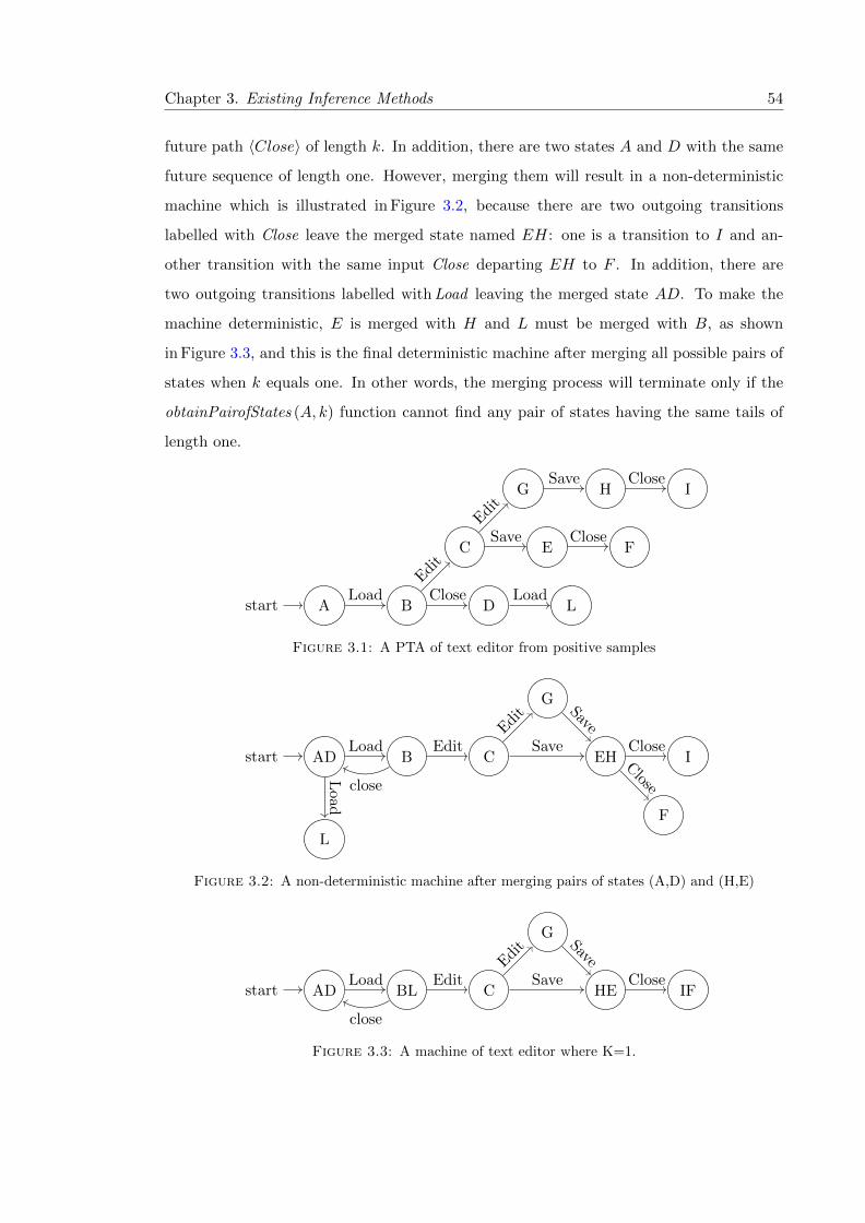
Chapter 3. Existing Inference Methods 54
future path 〈Close〉 of length k. In addition, there are two states A and D with the same
future sequence of length one. However, merging them will result in a non-deterministic
machine which is illustrated in Figure 3.2, because there are two outgoing transitions
labelled with Close leave the merged state named EH: one is a transition to I and an-
other transition with the same input Close departing EH to F . In addition, there are
two outgoing transitions labelled with Load leaving the merged state AD. To make the
machine deterministic, E is merged with H and L must be merged with B, as shown
in Figure 3.3, and this is the final deterministic machine after merging all possible pairs of
states when k equals one. In other words, the merging process will terminate only if the
obtainPairofStates (A, k) function cannot find any pair of states having the same tails of
length one.
Astart B
C
D
G
E
H I
F
LLoad
Edit
Close
Edit
Save
Save Close
Close
Load
Figure 3.1: A PTA of text editor from positive samples
ADstart B C
G
EH I
F
L
Load Edit
close
Edit
Save
Save
Close
Close
Load
Figure 3.2: A non-deterministic machine after merging pairs of states (A,D) and (H,E)
ADstart BL C
G
HE IFLoad Edit
close
Edit
Save
Save
Close
Figure 3.3: A machine of text editor where K=1.

Chapter 3. Existing Inference Methods 55
It is important to mention that the key factor in the k -tails algorithm is the value of k.
There is no systematic way to pick the value of k, it is essentially based upon developer
judgement [42]. If the value of k is big, many states are not merged together. In contrast,
if it is very low, the inferred machine will be over-generalized because it is likely to merge
non-equivalent states [42]. Lo et al. [70] stated that if there is a very limited number of
traces (sparseness), the value of k should be small in order to mine good generalization
models.
Walkinshaw and Bogdanov [45] stated that a pair of states may be inequivalent if they
have the same suffixes of length k. Moreover, a pair of states that do not match the same
suffixes of length k may not be different, especially in situations where training data is
sparse [45].
To sum up, the poor performance of the k -tails algorithm is not surprising since it is
only working with positive traces, which are not adequate to infer an accurate LTSs [45].
Moreover, inferring state-machine models from execution traces using the k -tails algo-
rithm may produce imprecise models that contain wrong behaviours [41, 98]. According
to Walkinshaw and Bogdanov [45] the absence of negative traces causes the learning process
to fail to stop over-generalizing LTSs by avoiding invalid mergers [45].
3.1.2 Experiments Using k-tails
We ran a small experiment to express the effect of k values on the inferred LTSs using
the k -tails algorithm. Series of random LTSs were generated for each number of states
ranging between 5 and 50 in steps of five. In other words, 15 different LTSs were randomly
generated for each chosen number of states (10 steps * 15= 150 LTSs in total). The size of
alphabet is given by Σ = |Q|×2. The Forest Fire algorithm that is described in Section 2.6
was used to generate random LTSs. The reason behind learning this number of LTSs is
to assess the performance of various algorithms on random LTSs with different traces fed
to each LTS. In addition, the randomly generated LTSs were connected.
For each LTS two sets of training data were generated, bringing the number of LTSs learnt
per experiment to 300. The generated LTSs were initially connected, had alphabet size 2x
the number of states. In this experiment, a set of positive traces (training sequences) was
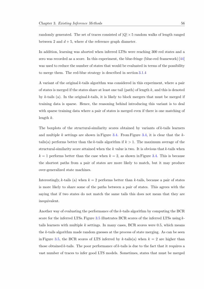
Chapter 3. Existing Inference Methods 56
randomly generated. The set of traces consisted of |Q| × 5 random walks of length ranged
between 2 and d+ 5, where d the reference graph diameter.
In addition, learning was aborted when inferred LTSs were reaching 300 red states and a
zero was recorded as a score. In this experiment, the blue-fringe (blue-red framework) [44]
was used to reduce the number of states that would be evaluated in terms of the possibility
to merge them. The red-blue strategy is described in section 3.1.4
A variant of the original k -tails algorithm was considered in this experiment, where a pair
of states is merged if the states share at least one tail (path) of length k, and this is denoted
by k -tails (a). In the original k -tails, it is likely to block mergers that must be merged if
training data is sparse. Hence, the reasoning behind introducing this variant is to deal
with sparse training data where a pair of states is merged even if there is one matching of
length k.
The boxplots of the structural-similarity scores obtained by variants of k -tails learners
and multiple k settings are shown in Figure 3.4. From Figure 3.4, it is clear that the k -
tails(a) performs better than the k -tails algorithm if k > 1. The maximum average of the
structural-similarity score attained when the k value is two. It is obvious that k -tails when
k = 1 performs better than the case when k = 2, as shown in Figure 3.4. This is because
the shortest paths from a pair of states are more likely to match, but it may produce
over-generalized state machines.
Interestingly, k -tails (a) when k = 2 performs better than k -tails, because a pair of states
is more likely to share some of the paths between a pair of states. This agrees with the
saying that if two states do not match the same tails this does not mean that they are
inequivalent.
Another way of evaluating the performance of the k -tails algorithm by computing the BCR
score for the inferred LTSs. Figure 3.5 illustrates BCR scores of the inferred LTSs using k -
tails learners with multiple k settings. In many cases, BCR scores were 0.5, which means
the k -tails algorithm made random guesses at the process of state merging. As can be seen
in Figure 3.5, the BCR scores of LTS inferred by k -tails(a) when k = 2 are higher than
those obtained k -tails. The poor performance of k -tails is due to the fact that it requires a
vast number of traces to infer good LTS models. Sometimes, states that must be merged
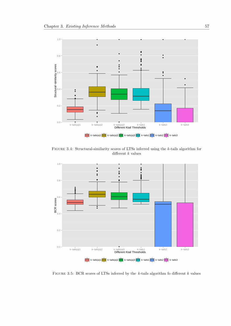
Chapter 3. Existing Inference Methods 57
0.0
0.2
0.4
0.6
0.8
1.0
k−tails(a)1 k−tails(a)2 k−tails(a)3 k−tails1 k−tails2 k−tails3Different Ktail Thresholds
Str
uctu
ral−
sim
ilarit
y sc
ores
k−tails(a)1 k−tails(a)2 k−tails(a)3 k−tails1 k−tails2 k−tails3
Figure 3.4: Structural-similarity scores of LTSs inferred using the k -tails algorithm fordifferent k values
0.0
0.2
0.4
0.6
0.8
1.0
k−tails(a)1 k−tails(a)2 k−tails(a)3 k−tails1 k−tails2 k−tails3Different Ktail Thresholds
BC
R s
core
s
k−tails(a)1 k−tails(a)2 k−tails(a)3 k−tails1 k−tails2 k−tails3
Figure 3.5: BCR scores of LTSs inferred by the k -tails algorithm fo different k values

Chapter 3. Existing Inference Methods 58
using k -tails are ignored; this is because states do not have identical paths, as training
data is not complete and some paths that should exist are missing.
Therefore, to sum up, there is a slight improvement made by k -tails(a) compared to k -tails.
This is because training data is sparse and it is not likely to have identical paths of length
k leaving the equivalent states. In this way, k -tails(a) merges a pair of states if there is at
least one match between paths of length k leaving both states.
3.1.3 Variants of the k-tails
Variants of the k -tails algorithm have been investigated in the literature. Cook and Wolf
[49] stated that the original k -tails may be unrolling a loop of a sequence of event e =
〈e1, e2, e3, e4〉 and producing non-deterministic automaton, and this is due to the value
of k = 2. Hence, Cook and Wolf [49] modified the algorithm to handle rolling loops by
removing non-determinism . On the other hand, Miclet [108] introduced a technique to
infer a regular language from positive samples, which is called tail-clustering and can be
seen as a generalization version of k -tails [108]. In the tail-clustering algorithm, states are
merged based on the similarities in their sets of k -tails. These similarities are determined
using a distance metric where a pair of states is merged if the distance metric between the
set of tails is less than a certain limit.
Several attempts have been made to adapt the k -tails algorithm to infer different kinds
of automata. Lorenzoli et al. [39] described the GK-tail to infer Extended Finite State
Machines (EFSMs) that have context variables between interaction traces, that can be
used in EFSMs testing since it increases program comprehension and analysis [39]. This
algorithm relies on many positive samples of traces, and generates an (EFSMs) in four
steps.
First, the GK-tail algorithm receives a set of traces that are augments with variables,
and called input-equivalent traces. Those traces are equivalents since they have the same
(sharing) events calls or methods invocations, and differ in data value of inputs. In this
case, the GK-tail learner merges those similar input-equivalent traces into a single one that
is annotated with multiple values of data [40]. Second, GK-tail produces predicates as con-
straints that are derived from data values and are associated with traces. Third, GK-tail
constructs the initial EFSM by building the tree from the merged traces that is achieved
Chapter 3. Existing Inference Methods 59
in the first step. The initial EFSM is annotated with the derived predicates. Fourth,
GK-tail learner iteratively merges equivalent states to infer the consistent EFSM to the
observed traces. For each pair of states, GK-tail compares the future paths in the length
k in the same way as the k -tails learner to decide which states are to be merged. Lorenzoli
et al. [39] introduced an equivalent criterion where pairs of states are merged if they have
the same k-paths of events and the constraints allocated to transitions. Sometimes [39],
the traces may be incomplete, and in this case two different merging criteria are proposed:
weakly subsumes, and strongly subsumes.
Another variant of the k -tails learner was proposed by Raman et al. [109] to infer proba-
bilistic finite state automata (PFSA), which is called sk-strings. This is may be defined
as strings that are considered as k -tails, but they do not have to end at terminated states,
unless they are less than the specified k value [109]. In other words, the set of k-string is
defined in Definition 3.1.
Definition 3.1. [109] The k-string is defined as {w|w ∈ Σ∗, |w| = k ∧ δ(q, w) ⊂ Q∨ |w| <
k ∧ δ(q, w) ∩ Fc 6= ∅}. Where Fc is the set of leaves nodes in the PTA.
In sk-strings [109], the notion of top s% was introduced to denote the most probable k-
strings that can be generated from a state. Thus, two states are merged on the condition
that they are indistinguishable for the most probable k-string [98, 109]. Only k-strings with
probabilities up to s% will be considered during evaluating the decision of merging states.
That is, two states are said to be mergeable if the sets of k-strings for both states share
the top s% of their k-strings. The resulting PFSA is over-generalized if s% is small [109].
In addition, the Sk-strings method requires all k-strings of both states to be the same if
s = 100%.
3.1.4 Evidence-Driven State Merging
This section introduces one of the most successful passive inference techniques known as
evidence-driven state merging (EDSM). The EDSM learner [44] won the Abbadingo one
DFA learning competition. It can be seen as a refinement of the RPNI algorithm. The
name of the EDSM algorithm reflects its purpose, it uses heuristic evidence (a score) to
evaluate each potential pair of states before merging them.

Chapter 3. Existing Inference Methods 60
In the EDSM learner, each pair of states is given a score, and is computed by counting the
number of states that are merged if the merging process is performed. That is, the score
that is assigned to a possible merge is obtained by counting the total number of states that
would be merged with others states [36, 44, 110]. This score can be called a compatibility
score or an EDSM score.
The idea behind computing the EDSM score is to measure the likelihood that a pair of
states is equivalent. Hence, the EDSM learner gives preference to a pair of states with
the highest score to be merged first [44, 111]. The key advantage of implementing EDSM
is that possible pairs in a specific boundary are evaluated before selecting the most likely
pair to be merged based on its score. Possible pairs of states are prioritized (ranked) from
the highest to the lowest scores. A pair of states with the highest score is merged first.
Unlike the k-tails algorithm that relies on merging the first pair of states that share the
same set of tails of length k, the EDSM learner relies on computing scores for possible
pairs of states, and then picks one of them for merging [45].
Additionally, the EDSM algorithm assigns a negative score to each pair of states that
cannot be merged. Merging of an accepting state with a rejecting state is not allowed
by the EDSM learner (see definition in 3.2). In this situation, EDSM assigns a negative
score denoting that a pair of states is unmergeable. Moreover, any states that would
be merged recursively during the determinization process must be compatible to avoid
merging a rejecting state with an accepting one, and vice versa. That is, a merge of two
states (q1, q2) is rejected if there is a transition a from a state q1 leads to a rejecting state
δ(q1, a) ∈ F−, and there is another transition with the same label a leaving a state q2
reaches an accepting state δ(q2, a) ∈ F+.
Definition 3.2. Given a pair of states (q1, q2) ∈ Q and APTA(A). A merge of (q1, q2) is
rejected by the EDSM iff q1 ∈ F+, q2 ∈ F− and vice versa.
Example 3.2. Consider the text editor example that is illustrated in Figure 3.6; the EDSM
learner would assign a score of 4 to the pair of B and C, and a score of -1 to denote that
the pair of B and D is not compatible because merging of an accepting state C with a
non-accepting one N is blocked.
To reduce the search space of evaluating possible pairs of states that can be merged, the
red-blue technique [44] can be applied with EDSM. The red-blue strategy is sometimes

Chapter 3. Existing Inference Methods 61
Astart B
C
D
G
E
H I
F
N
KO
Load
Close
Edit
Close
Edit
Save
Save Close
Close
Edit
Load
Figure 3.6: An APTA in the red-blue algorithm
called the blue-fringe strategy. Basically, the red-blue technique begins by colouring the
root state of an APTA red and all adjoining nodes are made blue [44]. Then, the possibility
of merging every blue state to the red states is measured using the EDSM score. If a red-
blue pair of states cannot be merged, the EDSM assigns a negative score. Once a blue state
cannot merge with any red state, it is coloured red and its children nodes then become
blue, as illustrated in Figure 3.6. This process is performed until all nodes in the tree are
coloured red. The whole body of the EDSM algorithm is provided in Algorithm 5.
The EDSM algorithm starts by invoking the generatePTA (S+, S−) function to construct
the initial APTA in line 1. In addition, the generalization threshold π should be initialized
before starting the inference process. A pair of states with a EDSM score above or equal
π is considered for merging. After that, the red-blue strategy is invoked to colour the root
of the PTA red, and its children non-red states are coloured blue. The process of making
the non-red state blue is performed using the ComputeBlue(A,R) function in Algorithm 5.
The computation of blue states is defined formally in Definition 3.3 where B denotes the
set of blue states and R denotes the set of red states.
Definition 3.3.
ComputeBlue(B) = {q1 ∈ QA | for some q ∈ R and σ ∈ Σ, such that q1 = δ(q, σ)
and q1 /∈ R}
The term blue boundary is also used to refer to the set of blue states that neighbour the red
states. The EDSM algorithm then iterates through the set of blue states to evaluate the
ability of merging them with red states as shown in lines 9-22. For each pair of red/blue

Chapter 3. Existing Inference Methods 62
input : S+, S−
/* Sets of accepted S+ and rejected S− sequences */
result: A is an LTS that is compatible with S+ and S−
Data: A,R,B,PossiblePairs
1 A← generatePTA (S+, S−);2 π ← 0;/* This parameter */
3 R← {q0} ; // R is a set of red states
4 do5 do6 PossiblePairs← ∅ ; // PossiblePairs possible pairs to merge
7 Rextended← false ;8 B ← ComputeBlue(A,R) ; // B is a set of blue states
9 for qb ∈ B do10 mergeable← false ;11 for qr ∈ R do12 EDSMScore← computeEDSMScore (A, qr, qb);13 if EDSMScore ≥ π then14 PossiblePairs← PossiblePairs ∪ {(qr, qb)} ;15 mergeable← true ;
16 end
17 end18 if mergeable = false then19 R← R ∪ {qb};20 Rextended← true ;
21 end
22 end
23 while Rextended = true;24 if PossiblePairs 6= ∅ then25 PairToMerge← PickPair (PossiblePairs);26 A← Merge (PairToMerge);
27 end
28 while PossiblePairs 6= ∅;29 return A
Algorithm 5: The EDSM inference algorithm
states, the EDSM learner calls the computeEDSMScore(A, qr, qb) function to count the
number of states that may be eliminated if merging them is performed. Once the EDSM
score is computed, the pair of states are added to the PossiblePairs set if the allocated
score is higher or equal to π, as shown in line 14, and the blue state is marked as mergeable.
Furthermore, if a blue state is unmergeable with any red state, it is added to the R set,
and its children states become blue. The process is then iterated to evaluate the new blue
states with each red state.

Chapter 3. Existing Inference Methods 63
The PickPair(PossiblePairs) function is responsible for picking the pair of states with the
highest score, and it is passed to merge the states in the pair using the Merge (PairToMerge)
function. The inference process is continued with the same procedure until all states are
coloured red. In other words, the process is terminated when the PossiblePairs set is
empty.
It is important to emphasise that the EDSM learner expected to have positive and negative
sequences in order to generalize the LTS models under the control of negative sequences.
Walkinshaw et al. [100] suggested variants of the EDSM learner by introducing the gen-
eralization (merging) threshold. It is introduced to block merging of a pair of states with
a score below the generalization threshold.
In the absence of negative samples, the merging threshold can be used to mitigate the
over-generalization problem. However, this solution tends to be useless since it is difficult
to pick the appropriate threshold for the provided traces. In addition, it may arbitrarily
block states that should be merged.
It is important to point out that the EDSM learner fails to infer an exact LTS model for two
reasons. First, training data are often too sparse to accumulate sufficient evidence about
correct merges of states [112, 113]. Second, the absence or the amount of negative samples
does not help the inference process to avoid over-generalization. If negative samples are not
available, false merges will be more likely to happen [114]. In addition, the only restriction
to avoid bad mergers is the compatibility constraint (avoiding merging accepted states with
rejecting ones and vice versa), which is not enough if there are few negative traces [110].
3.1.5 Experiments Using EDSM
In order to evaluate the efficiency of the EDSM algorithm when alphabet size is large, the
same experiments that are described in Section 3.1.1 were conducted for different variants
of the EDSM algorithm. In cases where only positive traces were considered, the total
number of sequences is given by |Q|×5. In this section, another experiment was conducted
to study the impact of negative traces. Therefore, the total number of traces is |Q| × 5
where half of the sequences were positive and the other half were negative.

Chapter 3. Existing Inference Methods 64
Figure 3.7 shows two groups of box-plots representing the BCR scores of the inferred LTSs
in two cases. First, if only positive samples are included in the inference process (the right
group of box-plots), and second if negative samples are provided with positive ones (the
left group of box-plots).
0.0
0.2
0.4
0.6
0.8
1.0
Positive and Negative Positive OnlyDifferent EDSM Thresholds
BC
R s
core
s
EDSM>=0 EDSM>=1 EDSM>=2 EDSM>=3 EDSM>=4
Figure 3.7: BCR scores obtained using the EDSM algorithm for different EDSM thresh-old values
The right group consists of different box-plots representing the BCR scores of LTSs inferred
using different EDSM learners from positive sequences only. From Figure 3.7 we can see
that EDSM over-generalizes LTSs when the threshold is set to zero or one; this is due to
the absence of negative samples that can control the generalization by preventing many
incorrect mergers. The horizontal line in the right group in Figure 3.7 shows that the BCR
values are 0.5, which indicates that the learner makes random guesses of states merging
(over-generalization).
In the absence of negative samples, one may constrain the merging process by increasing
the threshold to two, three, and four. Figure 3.7 illustrates that when the threshold is
three, the average BCR is around 0.67. However, EDSM under-generalizes LTSs when the
threshold is greater than 2; this means many states are blocked from being merged, which
is considered bad during the generalization process.

Chapter 3. Existing Inference Methods 65
As noted by Walkinshaw et al. [100], the accuracy of the inferred models becomes very
low when the merging threshold is low compared to that with a high threshold. Moreover,
with a very low threshold, the language of the inferred models accept many false positive
sequences. The study in this section agrees with their findings [100] in which the BCR
scores can be improved by increasing the EDSM threshold from two to three.
The left group of box-plots shown in Figure 3.7 summarizes the BCR scores attained by
variants of the EDSM algorithm in cases where positive and negative sequences were sup-
plied. In comparison to the case when only positive samples are provided, the figures show
that EDSM performs better if negative samples are available and the merging threshold is
one or two. For instance, the average BCR scores of LTSs inferred when negative samples
are available and the threshold is zero is 0.60 compared to 0.5 in cases of positive samples
only.
0.0
0.2
0.4
0.6
0.8
1.0
Positive and Negative Positive OnlyDifferent EDSM Thresholds
Str
uctu
ral−
sim
ilarit
y sc
ores
EDSM>=0 EDSM>=1 EDSM>=2 EDSM>=3 EDSM>=4
Figure 3.8: Structural-similarity scores of LTSs inferred using the EDSM algorithm fordifferent EDSM threshold values
Additionally, the impact of the EDSM threshold on the structural-similarity scores of
the inferred LTSs using EDSM is illustrated in Figure 3.8. In cases where only positive
sequences are provided and the merging threshold is one or two, the average structural-
similarity score of inferred LTSs are zero; this denotes that the models are over-generalized.

Chapter 3. Existing Inference Methods 66
It is clear that the structural-similarity scores achieved by learners are very sensitive to
the existence of negative samples and the settings of the EDSM threshold. The average
structural-similarity scores attained by EDSM is nearly 0.5 when the threshold is three,
which is higher than others obtained by different settings of the EDSM threshold.
During the conducted experiments, the ratio of correctness for the number of states was
computed as follows:
ratio of correctness =The number of states of LTSs inferred using a learner
The number of states of the target LTSs(3.1)
The ratio of correctness for the number of states of LTSs inferred using different EDSM
learners are shown in Figure 3.9. It is apparent from Figure 3.9 that the number of states
is affected by the setting of the EDSM threshold. As shown in Figure 3.9, the EDSM
learner generates LTSs with the number of states close to those in the hidden target LTSs
when the EDSM threshold equals two. From Figure 3.9, the figures indicate that many
mergers are not made that should be when the threshold is three or four. This indicates
that the setting of the EDSM threshold is critical.
In situations where positive and negative sequences are provided, the number of states is
affected by the setting of the EDSM threshold, as shown in Figure 3.10. It is apparent
that the inferred LTSs have more states compared to the target LTSs if the threshold is
set to three or four. On the other hand, the numbers of states of the inferred models are
so close to the target LTSs when the EDSM threshold is two.
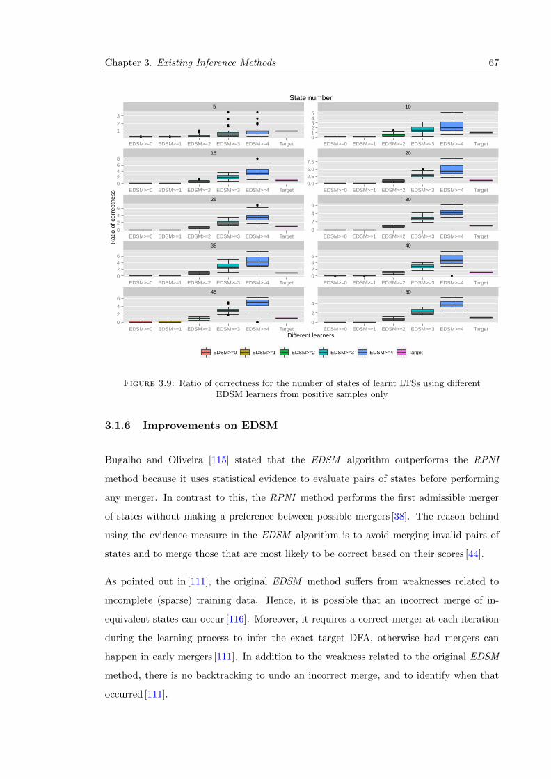
Chapter 3. Existing Inference Methods 67
5 10
15 20
25 30
35 40
45 50
1
2
3
012345
02468
0.02.55.07.5
0246
0
2
4
6
0246
0246
0
2
4
6
0
2
4
EDSM>=0 EDSM>=1 EDSM>=2 EDSM>=3 EDSM>=4 Target EDSM>=0 EDSM>=1 EDSM>=2 EDSM>=3 EDSM>=4 Target
EDSM>=0 EDSM>=1 EDSM>=2 EDSM>=3 EDSM>=4 Target EDSM>=0 EDSM>=1 EDSM>=2 EDSM>=3 EDSM>=4 Target
EDSM>=0 EDSM>=1 EDSM>=2 EDSM>=3 EDSM>=4 Target EDSM>=0 EDSM>=1 EDSM>=2 EDSM>=3 EDSM>=4 Target
EDSM>=0 EDSM>=1 EDSM>=2 EDSM>=3 EDSM>=4 Target EDSM>=0 EDSM>=1 EDSM>=2 EDSM>=3 EDSM>=4 Target
EDSM>=0 EDSM>=1 EDSM>=2 EDSM>=3 EDSM>=4 Target EDSM>=0 EDSM>=1 EDSM>=2 EDSM>=3 EDSM>=4 TargetDifferent learners
Rat
io o
f cor
rect
ness
EDSM>=0 EDSM>=1 EDSM>=2 EDSM>=3 EDSM>=4 Target
State number
Figure 3.9: Ratio of correctness for the number of states of learnt LTSs using differentEDSM learners from positive samples only
3.1.6 Improvements on EDSM
Bugalho and Oliveira [115] stated that the EDSM algorithm outperforms the RPNI
method because it uses statistical evidence to evaluate pairs of states before performing
any merger. In contrast to this, the RPNI method performs the first admissible merger
of states without making a preference between possible mergers [38]. The reason behind
using the evidence measure in the EDSM algorithm is to avoid merging invalid pairs of
states and to merge those that are most likely to be correct based on their scores [44].
As pointed out in [111], the original EDSM method suffers from weaknesses related to
incomplete (sparse) training data. Hence, it is possible that an incorrect merge of in-
equivalent states can occur [116]. Moreover, it requires a correct merger at each iteration
during the learning process to infer the exact target DFA, otherwise bad mergers can
happen in early mergers [111]. In addition to the weakness related to the original EDSM
method, there is no backtracking to undo an incorrect merge, and to identify when that
occurred [111].

Chapter 3. Existing Inference Methods 68
5 10
15 20
25 30
35 40
45 50
2
4
6
2468
0369
0369
0.0
2.5
5.0
7.5
0.02.55.07.5
0.02.55.07.5
0246
0246
0
2
4
6
EDSM>=0 EDSM>=1 EDSM>=2 EDSM>=3 EDSM>=4 Target EDSM>=0 EDSM>=1 EDSM>=2 EDSM>=3 EDSM>=4 Target
EDSM>=0 EDSM>=1 EDSM>=2 EDSM>=3 EDSM>=4 Target EDSM>=0 EDSM>=1 EDSM>=2 EDSM>=3 EDSM>=4 Target
EDSM>=0 EDSM>=1 EDSM>=2 EDSM>=3 EDSM>=4 Target EDSM>=0 EDSM>=1 EDSM>=2 EDSM>=3 EDSM>=4 Target
EDSM>=0 EDSM>=1 EDSM>=2 EDSM>=3 EDSM>=4 Target EDSM>=0 EDSM>=1 EDSM>=2 EDSM>=3 EDSM>=4 Target
EDSM>=0 EDSM>=1 EDSM>=2 EDSM>=3 EDSM>=4 Target EDSM>=0 EDSM>=1 EDSM>=2 EDSM>=3 EDSM>=4 TargetDifferent learners
Rat
io o
f cor
rect
ness
EDSM>=0 EDSM>=1 EDSM>=2 EDSM>=3 EDSM>=4 Target
stateNumber
Figure 3.10: Ratio of correctness for the number of states of learnt LTSs using differentEDSM learners from positive and negative samples
Various research studies [111, 115] have attempted to improve the performance of the
EDSM learner with respect to the search procedure to the inference process. They [111,
115] aimed to increase the quality of the inferred models by exploring the tree (APTA) to
consider other possible state merges alongside those determined by the greedy search of
the EDSM learner. The following search techniques were used in the literature:
� The evidence-driven backtrack search (ED-BTS) is an improvement to the EDSM
algorithm that applies the backtracking search to the last merger if there is another
possible (alternative) merge [115]. Unfortunately, this backtrack method does not
significantly improve the inferred machines compared to the normal EDSM as stated
by Bugalho and Oliveira [115].
� Lang [117] proposed the evidence-driven beam search (ED-BEAM) algorithm, and
developed it by combining the beam search techniques with the heuristic strategy
used in the EDSM algorithm. The ED-BEAM algorithm starts by trying all possible
merging choices close to the root of tree, and then applies a heuristic search to select

Chapter 3. Existing Inference Methods 69
the best choice. The reason for using beam search strategy is to avoid earlier wrong
merge states made by a heuristic search [115, 117]. Lang [117] stated that ED-BEAM
is applicable for larger state machines inference.
� The evidence-driven stochastic search (ED-SS) [115] algorithm is designed to find the
state-merge (decision) that is very likely to be a bad merge. It uses a special mea-
surement that is computed to each possible merge of states, and this measurement
calculates the effect of merging two states on alternative possible merges. The score
is computed for each merge based on three scores [115].
To sum up, Bugalho and Oliveira [115] have investigated the performance of the above-
mentioned three variates of EDSM and concluded that there is a slight improvement
made by ED-BEAM and ED-SS compared to EDSM, which is not significant as claimed
by Bugalho and Oliveira [115].
3.1.7 Other Improvements
Lang et al. [44] suggested considering only merging pairs of states that lie within a specific
distance (window) from the root. This aimed to speed up the time of running the EDSM
algorithm. The W-EDSM algorithm performs faster than EDSM since it reduce the search
space during selecting pairs of states. Unfortunately, it leads to bad performance because
it misses deep pairs of states that have the highest scores.
Cicchello and Kremer [113] described the windowed EDSM (W-EDSM) as follows. In the
current hypothesis, make a window w of states in breadth-first order starting from the
root node. The size of the window w is set to be twice the size of the target machine.
Then, each pair of states within the distance w is evaluated, and the pair of states that has
the highest scores is merged. Once the size of the window is decreased after performing
merges, further states will be considered in the windows to make sure its size becomes
twice the target state machine. If there is no possible merge within the given distance w,
the size of the window is increased by two. The process is terminated when no further
merges are possible [112, 113]. Recently, Heule and Verwer [110] showed an improvement
to the EDSM learner in order to improve the inferred LTSs by introducing a new constraint
named a consistency check, which is described in the following sections.

Chapter 3. Existing Inference Methods 70
3.1.8 Introduction of Satisfiability to the State-Merging Strategy
Heule and Verwer [110] proposed a novel technique to synthesize software models. Their
algorithm is called DFASAT which is based on satisfiability (SAT) and a greedy technique
which is represented by the EDSM learner. Heule and Verwer [118] proposed using an
exact translation of DFA identification into SAT instances [119]. The SAT solver is then
used to find optimal DFA solutions. Initially, the inference process using DFASAT begins
with several steps of EDSM to minimize the inference problem before implementing the
SAT solver. Section 3.1.9 describes the consistency constraint proposed by Heule and
Verwer [110]. After that, the DFASAT algorithm is described in Section 3.1.11.
3.1.9 Heule and Verwer Constraint on State Merging
Heule and Verwer [110] showed a very interesting constraint during the inference method
using EDSM, where mergers are blocked if the merging process step adds new transitions to
a red state. This constraint is called consistency check, and developed with an assumption
that the red states are identified as correct states in the hidden target LTSs [110]. In this
way, a merge is not permitted to add new labels of the outgoing transitions from a blue
state to a red state [110]. The reason for blocking such mergers is an assumption that
considers red states to be correctly identified parts of the target model [110]. We refer to
this idea as Sicco’s idea. The Sicco’s idea can be implemented for only the considered pair
to merge, which is further referred to as SiccoN. It is important to highlight that SiccoN
is a variant of the EDSM leaner without any threshold. In this way, SiccoN only block
mergers when the EDSM score is below zero.
Example 3.3. Consider a merging of A and B in the PTA shown in Figure 3.11 is assumed
to be an invalid merge because the blue state B would add Close and Edit labels to the
red state A.
3.1.10 Experiments Using SiccoN
In order to evaluate the benefit of adding Sicco’s idea to the EDSM learner, the same
experiments that are described in Section 3.1.5 were conducted to measure the impact of
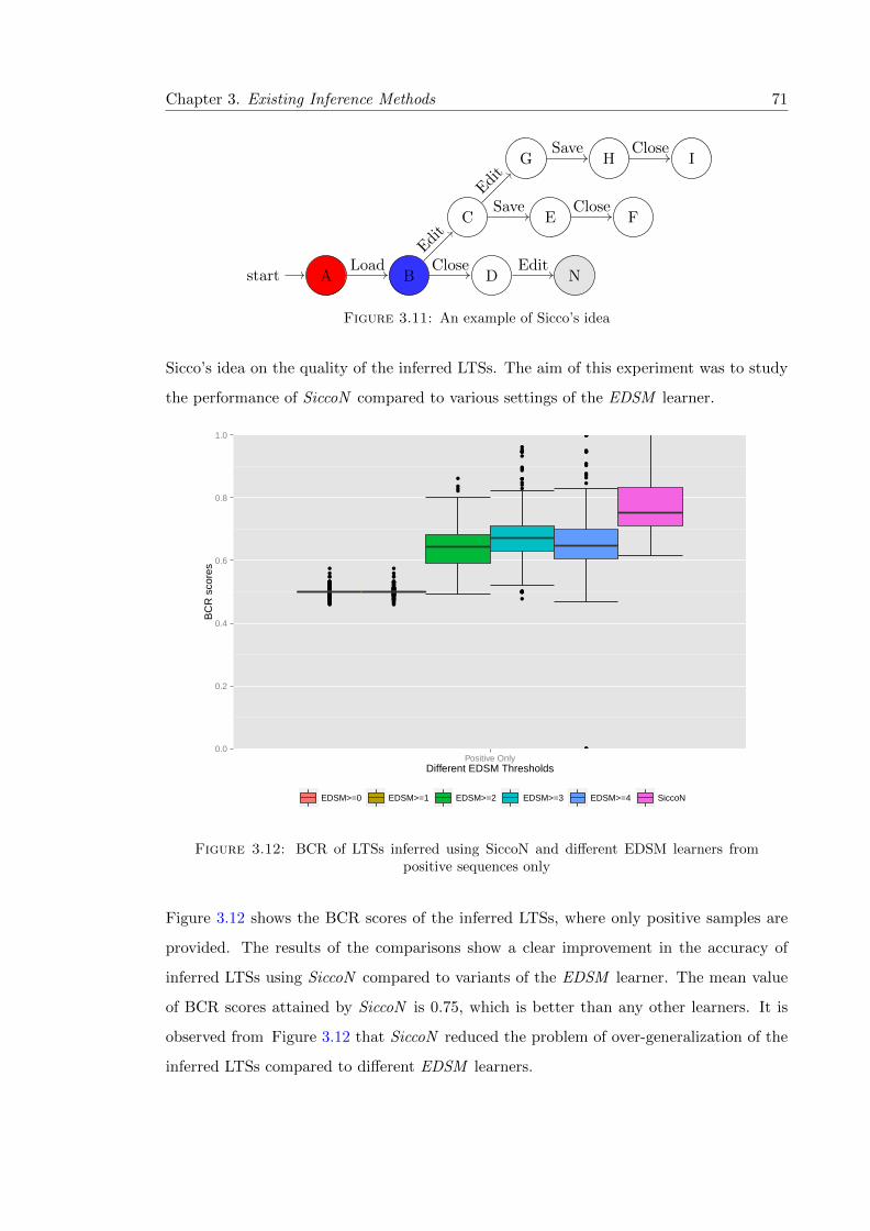
Chapter 3. Existing Inference Methods 71
Astart B
C
D
G
E
H I
F
NLoad
Edit
Close
Edit
Save
Save Close
Close
Edit
Figure 3.11: An example of Sicco’s idea
Sicco’s idea on the quality of the inferred LTSs. The aim of this experiment was to study
the performance of SiccoN compared to various settings of the EDSM learner.
0.0
0.2
0.4
0.6
0.8
1.0
Positive OnlyDifferent EDSM Thresholds
BC
R s
core
s
EDSM>=0 EDSM>=1 EDSM>=2 EDSM>=3 EDSM>=4 SiccoN
Figure 3.12: BCR of LTSs inferred using SiccoN and different EDSM learners frompositive sequences only
Figure 3.12 shows the BCR scores of the inferred LTSs, where only positive samples are
provided. The results of the comparisons show a clear improvement in the accuracy of
inferred LTSs using SiccoN compared to variants of the EDSM learner. The mean value
of BCR scores attained by SiccoN is 0.75, which is better than any other learners. It is
observed from Figure 3.12 that SiccoN reduced the problem of over-generalization of the
inferred LTSs compared to different EDSM learners.

Chapter 3. Existing Inference Methods 72
0.0
0.2
0.4
0.6
0.8
1.0
Positive and NegativeDifferent EDSM Thresholds
BC
R s
core
s
EDSM>=0 EDSM>=1 EDSM>=2 EDSM>=3 EDSM>=4 SiccoN
Figure 3.13: BCR attained by SiccoN and different EDSM learners from positive andnegative sequences
Figure 3.13 illustrates the BCR scores of the inferred LTSs using various learners, where
both positive and negative sequences were used to complete the inference process. The
obtained LTSs using SiccoN are good hypotheses compared to their target LTSs. The
median value of BCR scores attained by SiccoN is about 0.72, which is higher than any
other learners.
It is important to compare between SiccoN and EDSM learners in terms of the structural-
similarity scores. A boxplot of the structural-similarity scores of LTSs inferred from en-
tirely positive sequences using different learners are shown in Figure 3.14. It appears
that structural-similarity scores obtained by SiccoN are higher than those attained by the
EDSM learners. That is, SiccoN infers LTS models where their structures are closer to the
target LTSs than EDSM. On the other hand, the structural-similarity scores of inferred
LTSs from both positive and negative sequences are shown in Figure 3.15. The SiccoN
learner achieves the highest average of the structural-similarity scores compared to other
learners.
It is interesting to observe the number of states of the inferred LTSs from only positive
traces using SiccoN and EDSM. Hence, the ratio of correctness for the number of states

Chapter 3. Existing Inference Methods 73
0.0
0.2
0.4
0.6
0.8
1.0
Positive OnlyDifferent EDSM Thresholds
Str
uctu
ral−
sim
ilarit
y sc
ores
EDSM>=0 EDSM>=1 EDSM>=2 EDSM>=3 EDSM>=4 SiccoN
Figure 3.14: Structural-similarity scores achieved by SiccoN and different EDSM learn-ers from positive sequences only
0.0
0.2
0.4
0.6
0.8
1.0
Positive and NegativeDifferent EDSM Thresholds
Str
uctu
ral−
sim
ilarit
y sc
ores
EDSM>=0 EDSM>=1 EDSM>=2 EDSM>=3 EDSM>=4 SiccoN
Figure 3.15: Structural-similarity scores achieved by SiccoN and different EDSM learn-ers from positive sequences and negative

Chapter 3. Existing Inference Methods 74
5 10
15 20
25 30
35 40
45 50
1
2
3
012345
02468
0.02.55.07.5
0246
0
2
4
6
0246
0246
0
2
4
6
0
2
4
EDSM>=0 EDSM>=1 EDSM>=2 EDSM>=3 EDSM>=4 SiccoN Target EDSM>=0 EDSM>=1 EDSM>=2 EDSM>=3 EDSM>=4 SiccoN Target
EDSM>=0 EDSM>=1 EDSM>=2 EDSM>=3 EDSM>=4 SiccoN Target EDSM>=0 EDSM>=1 EDSM>=2 EDSM>=3 EDSM>=4 SiccoN Target
EDSM>=0 EDSM>=1 EDSM>=2 EDSM>=3 EDSM>=4 SiccoN Target EDSM>=0 EDSM>=1 EDSM>=2 EDSM>=3 EDSM>=4 SiccoN Target
EDSM>=0 EDSM>=1 EDSM>=2 EDSM>=3 EDSM>=4 SiccoN Target EDSM>=0 EDSM>=1 EDSM>=2 EDSM>=3 EDSM>=4 SiccoN Target
EDSM>=0 EDSM>=1 EDSM>=2 EDSM>=3 EDSM>=4 SiccoN Target EDSM>=0 EDSM>=1 EDSM>=2 EDSM>=3 EDSM>=4 SiccoN TargetDifferent learners
Rat
io o
f cor
rect
ness
EDSM>=0 EDSM>=1 EDSM>=2 EDSM>=3 EDSM>=4 SiccoN Target
stateNumber
Figure 3.16: Ratio of correctness for the number of states of learnt LTSs using SiccoNvs. different EDSM learners from positive samples only
was computed using Equation 3.1. Figure 3.16 shows that the number of states of LTSs
inferred using various learners. It is clear that the number of states of LTSs inferred using
SiccoN is very close to the target LTSs. It is worth noting that the number of states
of the inferred models using EDSM learner when the merging threshold is two is close
to the target number of states. However, this does not mean that the inferred models
are good with respect to the BCR and structural-similarity scores. In other words, the
smallest models are not always better in terms of language and structure. On the contrary,
given positive and negative samples, numbers of states of the inferred LTSs using SiccoN
converge to the exact number of states in the target LTSs as shown in Figure 3.17.

Chapter 3. Existing Inference Methods 75
5 10
15 20
25 30
35 40
45 50
2
4
6
2468
0369
0369
0.0
2.5
5.0
7.5
0.02.55.07.5
0.02.55.07.5
0246
0246
0
2
4
6
EDSM>=0 EDSM>=1 EDSM>=2 EDSM>=3 EDSM>=4 SiccoN Target EDSM>=0 EDSM>=1 EDSM>=2 EDSM>=3 EDSM>=4 SiccoN Target
EDSM>=0 EDSM>=1 EDSM>=2 EDSM>=3 EDSM>=4 SiccoN Target EDSM>=0 EDSM>=1 EDSM>=2 EDSM>=3 EDSM>=4 SiccoN Target
EDSM>=0 EDSM>=1 EDSM>=2 EDSM>=3 EDSM>=4 SiccoN Target EDSM>=0 EDSM>=1 EDSM>=2 EDSM>=3 EDSM>=4 SiccoN Target
EDSM>=0 EDSM>=1 EDSM>=2 EDSM>=3 EDSM>=4 SiccoN Target EDSM>=0 EDSM>=1 EDSM>=2 EDSM>=3 EDSM>=4 SiccoN Target
EDSM>=0 EDSM>=1 EDSM>=2 EDSM>=3 EDSM>=4 SiccoN Target EDSM>=0 EDSM>=1 EDSM>=2 EDSM>=3 EDSM>=4 SiccoN TargetDifferent learners
Rat
io o
f cor
rect
ness
EDSM>=0 EDSM>=1 EDSM>=2 EDSM>=3 EDSM>=4 SiccoN Target
stateNumber
Figure 3.17: Ratio of correctness for the number of states of learnt LTSs using SiccoNvs. different EDSM learners from positive and negative samples
3.1.11 DFASAT Algorithm
The earlier study by Heule and Verwer [118] suggested the translation of the DFA inference
problem into satisfiability (SAT). This translation that has been used by Heule and Verwer
[118] is inspired by the previous translation of the DFA identification problem into the
graph colouring issue [120].
It is the problem of colouring nodes in the given graph where nodes connected with an edge
have a different colour, and sometimes is known as state colouring. The DFA identification
problem use the colouring graph such that compatible states in the same block are coloured
with the same colour, and those that cannot be merged are given different colours [120].
Heule and Verwer [118] have focused on translating the graph colouring strategy into SAT.
However, this translation can result in a huge number of clauses, which is too difficult for
the existing SAT solver. This explain why the DFASAT algorithm attempts to run EDSM
in the earlier steps before calling the SAT solver to complete the inference process and
avoiding handling the large number of clauses.
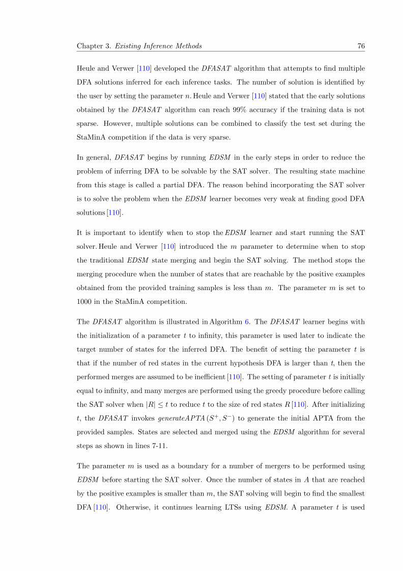
Chapter 3. Existing Inference Methods 76
Heule and Verwer [110] developed the DFASAT algorithm that attempts to find multiple
DFA solutions inferred for each inference tasks. The number of solution is identified by
the user by setting the parameter n. Heule and Verwer [110] stated that the early solutions
obtained by the DFASAT algorithm can reach 99% accuracy if the training data is not
sparse. However, multiple solutions can be combined to classify the test set during the
StaMinA competition if the data is very sparse.
In general, DFASAT begins by running EDSM in the early steps in order to reduce the
problem of inferring DFA to be solvable by the SAT solver. The resulting state machine
from this stage is called a partial DFA. The reason behind incorporating the SAT solver
is to solve the problem when the EDSM learner becomes very weak at finding good DFA
solutions [110].
It is important to identify when to stop the EDSM learner and start running the SAT
solver. Heule and Verwer [110] introduced the m parameter to determine when to stop
the traditional EDSM state merging and begin the SAT solving. The method stops the
merging procedure when the number of states that are reachable by the positive examples
obtained from the provided training samples is less than m. The parameter m is set to
1000 in the StaMinA competition.
The DFASAT algorithm is illustrated in Algorithm 6. The DFASAT learner begins with
the initialization of a parameter t to infinity, this parameter is used later to indicate the
target number of states for the inferred DFA. The benefit of setting the parameter t is
that if the number of red states in the current hypothesis DFA is larger than t, then the
performed merges are assumed to be inefficient [110]. The setting of parameter t is initially
equal to infinity, and many merges are performed using the greedy procedure before calling
the SAT solver when |R| ≤ t to reduce t to the size of red states R [110]. After initializing
t, the DFASAT invokes generateAPTA (S+, S−) to generate the initial APTA from the
provided samples. States are selected and merged using the EDSM algorithm for several
steps as shown in lines 7-11.
The parameter m is used as a boundary for a number of mergers to be performed using
EDSM before starting the SAT solver. Once the number of states in A that are reached
by the positive examples is smaller than m, the SAT solving will begin to find the smallest
DFA [110]. Otherwise, it continues learning LTSs using EDSM. A parameter t is used

Chapter 3. Existing Inference Methods 77
Require: an input sample of sequencesS = S+ ∪ S−, a test sample St, merge boundm, number of DFA solutions n, accepting vote percentage avp between 0and 1
Ensure : Label is a labelling for St aimed to give high accuracy for software models
1 Let t←∞2 Let D ← ∅ //D is a set of multiple DFAs solutions3 A = GenerateAPTA (S+, S−) //generate the APTA A from sequences4 while |D| < n do5 //while the number of DFA solution is less than n
6 Let A′ ← copyAPTA (A) // create another copy of APTA A
′
7 while |A′ |p < m do
8 //while the positive sequences reach more than m states in A′
9 select q and q′ in A′
using random greedy ;
10 A′
= merge (A′, q, q′) // merge states in A
′using random greedy
11 end
12 // if A′
has more than t red states
13 if |R| > t (R being the red states in A′) then
14 // find a better partial DFA solutioncontinue the next while loop iteration
15 end16 set t← |R| // else update t to the amount of resulting red states17 let i← 0 // initialize the number of additional states to 018 // while no solution has been found for the remaining problem19 while true do
20 translate A′
to a SAT formula using |R|+ i colours// try to find an exact solution with i extra states
21 solve the formula using a SAT-solver ;22 if the solver return a DFA solution A′′ then23 // if the SAT solver finds a solution add it to D24 add A′′ to D and break
25 else if the solver used more than 300 seconds A′′ then26 break // try another partial solution if the problem is too hard27 else28 set i← i+ 1 // else try to find a larger solution29 end
30 end
31 end32 let Label be an empty labeling // initialize the test labeling33 // iterating through test set St34 forall the s ∈ St do35 if |{A ∈ D|s ∈ L(A)}| ≥ avp then36 append ‘1’ to Label
// s is labelled as positive because at least avp % of the solutions accept s37 else38 append ‘0’ to Label // label s as negative39 end40 return Label
41 end
Algorithm 6: The DFASAT Algorithm [110]

Chapter 3. Existing Inference Methods 78
later to refer to a target size of a DFA [110]. Once the APTA becomes small, the APTA
is translated to many clauses and they are passed to the solver to find a DFA as shown in
lines 19-30. Every time a DFA is inferred, it will be added to the set D as shown in line
24. The reason behind collecting all possible solutions is to find the optimal generalization
of DFA using multiple DFA solutions using the ensemble method [121].
The DFASAT algorithm attempts to generate many DFA solutions. When a number of
DFA solutions are generated, the test sequences are passed to each DFA to decide which
of them are rejected or accepted. [110] introduced accepting vote percentage (avp) such
that if a test sequence is accepted by avp % of the generated DFA, then it is classified
as positive, and otherwise, it is classified as negative. This idea is motivated by the
ensemble method [121] to improve the classification accuracy and treating the problem of
data sparseness in the StaMinA competition.
3.1.12 Inferring State-Machine Models by Mining Rules
Lo et al. [6] described rule mining as the process of identifying constraint between the pre-
condition and post-condition of rules. In the last decade, rule mining from traces has gained
attention from software engineers looking to understand how a program behave [7, 23].
Interestingly, rule mining techniques can be used to steer state machine inference strate-
gies. Lo et al. [70] suggested the leveraging of two learning methods: rule mining and
automata inference to avoid the over-generalization problem. There are two phases in
their miner [70]. First, rule mining to statistically infer temporal properties between the
events in traces [70]. Those properties in the forms of the rules identified the relation
between the distant events in the traces [70]. The mined rules can be either future-time or
past-time rules. Future-time rules determine the relations or dependencies between events,
such that whenever a series of events occurs (appears in the traces), another sequence of
events must happen subsequently [70]. Past-time rules determine relations between events
such that whenever a sequence of events occurs, another sequence must happen before [70].
The second phase involves inferring automata with steering based on the mind rules in
the first step. In the second phase, Lo et al. [70] states are merged only if all the mined
rules are satisfied by the automata generated after the merging step. If the resulting
automaton violates the mined rules, then states are not merged. The evaluation of their

Chapter 3. Existing Inference Methods 79
approaches [70] showed that the accuracy of inferred automata using temporal rules can
be increased in terms of the precision scores.
In this thesis, it is of limited value to evaluate the proposed learner with such rule-mining
based approach. This is because the mined rules are represented as pre- and post-condition
pairs where the post condition is known to be held if the pre-condition is held based on the
confidence metric [70]. In the EDSM-Markov learner that is proposed in this thesis, EDSM-
Markov does not have any knowledge as to whether the proprieties are held in the target
system or not. Their approaches [70] allow users to modify, and delete the mined rules
while EDSM-Markov prevents the users intervention. The inference of state machine by
mining rules is applied with the k -tails algorithm. However, the performance can be poor
at inferring LTSs where there are few traces.

Chapter 3. Existing Inference Methods 80
3.2 Active Learning
In passive learning, the inference process attempts to generate an automaton model from
the provided traces. Unfortunately, traces might not contain sufficient information about
the behaviour of a system, and then it becomes difficult to learn an exact model from the
traces. The reason for this difficulty is that the provided traces cannot distinguish every
pair of states and are not able to identify equivalent states among a number of states.
Additionally, the performance of passive inference techniques is poor if the provided sam-
ples are sparse. An alternative approach was introduced to tackle the difficulties that have
faced passive learning techniques, and it is called the active learning strategy. Angluin
[79] introduced a powerful active learning algorithm named Lstar and it is denoted by
L∗. It is widely used in the grammar inference field to learn DFA models representing
a specific language from strings or sentences. Angluin [79] proved that an automaton can
be identified in polynomial time if the learning algorithm asks queries to collect missing
information to get exact models. In the L∗, there is a minimal adequate teacher (MAT)
responsible to answer specific kinds of queries that are posed by the inference learner.
In Angluin’s algorithm, two kinds of queries are posed to a teacher or an oracle: member-
ship queries and equivalence queries. In membership queries, the learner poses a sequence
S as a query to the oracle to decide whether it belongs to the language L. The answer
of membership queries is either accepted denoted as 1 indicating that a sequence over
Σ∗ belongs to the unknown language, or rejected denoted as 0 meaning that a sequence
does not belong to the target language. In equivalence queries, a query is asked to decide
whether an inferred model is isomorphic to the target model. If the answer of an equiv-
alence query is yes, then the state machine model is conjectured. Otherwise, a counter
example is returned in the form of membership queries. The answers are recorded as new
observations in a table called an observation table(OT).
In software model inference, the L∗ algorithm is aimed at exploring the system being
learnt by asking queries about its behaviour and returning the corresponding consistent
state machine models. It requires an oracle (a software system being inferred) to answer
queries. It requires interacting with the system under inference to collect observations by
asking queries.

Chapter 3. Existing Inference Methods 81
3.2.1 Observation Table
In Angluin’s algorithm, there is an assumption that the alphabet Σ is known. The L∗
incorporates the answered queries (sequences) in an observation table (OT). It is a specific
representation of an automaton in a table. All gathered sequences that are classified by
the posed queries are organized into the OT.
The OT is a 3-tuple OT = (S,E, T ) where rows S is a prefix-closed set of sequences over
Σ, columns E is a suffix-closed set of sequences over Σ, and T is a finite mapping function,
which maps ((S ∪ S · Σ) · E) to {0, 1} [79]. All sets (S, E) are assumed to be finite and
non-empty. Rows in the OT are labelled with (S ∪ S · Σ), and columns are labelled with
E. A cell in the OT is labelled with T (s · e), where s represents a row of the cell such that
s ∈ S ∪ S · Σ, and e is a column of the cell such that e ∈ E. Thus, T (s · e) is mapped to
1 if the sequence s · e belongs to the target DFA model, otherwise it is mapped to 0 to
denote the sequence s · e does not belong to the language. Table 3.1 illustrates an example
of the OT, where the set of alphabet is a, b.
Eε
S ε 1
S · Σ a 0b 0
Table 3.1: An example of the observation table
The equivalence of any two rows in the OT is identified based on the E set. Let s1, s2 ∈
S ∪ S ·Σ be a pair of rows, then s1 and s2 are equivalent, denoted by row(s1) =eq row(s2),
if and only if T (s1 · e) = T (s2 · e), ∀e ∈ E. An OT is called closed if ∀s1 ∈ S · Σ where
there exists s2 ∈ S such that row(s1) =eq row(s2). The OT is considered consistent as
long as s1, s2 ∈ S such that row(s1) =eq row(s2) and row(s1 · σ) =eq row(s2 · σ),∀σ ∈ Σ
3.2.2 L∗ Algorithm
The L∗ algorithm first constructs the table and initializes S = E = {ε}. Then, the
algorithm fills the OT to ensure the closed and consistent conditions by asking membership
queries for ε and each σ ∈ Σ. Once the OT is not consistent, the L∗ finds a pair of rows s1,
s2 ∈ S, σ ∈ Σ, and e ∈ E such that row(s1) =eq row(s2) where T (s1 · σ · e) 6= T (s2 · σ · e).

Chapter 3. Existing Inference Methods 82
The OT is extended by adding the sequence σ · e to E and asking membership queries to
fill missing information in (S ∈ S · Σ) · (σ · e) [79].
During the learning process, if the OT is not closed, then the L∗ algorithm attempts to
find s1 ∈ S ·Σ such that row(s1) 6=eq row(s2) for all elements of s2 ∈ S. The L∗ then adds
s1 to S. Then, the OT must be extended (expanded) by asking membership queries for
missing elements. This process is repeated until the OT becomes closed and consistent [79].
Once the OT is known to be consistent and closed, L∗ constructs the corresponding DFA
conjecture over Σ as follows:
� Q = {row(s) : s ∈ S}
� q0 = row(ε)
� F = {row(s) : s ∈ S and T (s) = 1}
� δ(row, σ) = row(s · σ)
The DFA conjecture may contain a small number of states in comparison with the target
size of the correct DFA. The L∗ passes the resulting conjecture to an oracle to check its
correctness against the target one. This is called an equivalent query and it requires an
answer from the oracle. If it replies yes this indicates that the conjecture is correct or it
returns a counterexample. The process will terminate if the answer is yes. However, if the
oracle returns with a counterexample, then the returned counterexample and its prefixes
are added into the set of S to extend the OT. Then, the OT is filled by asking membership
queries. The L∗ procedure is presented in Algorithm 7.

Chapter 3. Existing Inference Methods 83
input : A finite set of the alphabet Σresult: DFA conjecture M
1 S ← {ε}2 E ← {ε}3 OT ← (S,E, T )4 repeat5 while OT is not closed or not consistent do6 if OT is not closed then7 find s1 ∈ S · Σ such that row(s1) 6=eq row(s), ∀s ∈ S8 Move s1 to S;9 add s1 · a to S · Σ,∀a ∈ Σ;
10 Extend T to (S ∪S ·Σ) ·E by asking membership queries to fill the table
11 end12 if OT is not consistent then13 find s1, s1 ∈ S, σ ∈ Σ, and e ∈ E such that row(s1) =eq row(s2),14 but T (s1 · σ, e) 6= T (s2 · σ, e);15 add σ · e to E;16 Extend T to (S∪S ·Σ)·E by asking membership queries to fill the table;
17 end
18 end19 DFA← conjecture (OT )20 CE← FindEquivalenceQuery (DFA)21 if CE 6= φ then22 add CE and all the prefixes of CE to S23 Extend T to (S ∪ S · Σ) · E24 by asking membership queries to fill the table
25 end
26 until the oracle does not return any counterexample to DFA;
Algorithm 7: The L* Algorithm Following [79, 122]

Chapter 3. Existing Inference Methods 84
3.2.3 Example of L∗
In this section, an illustration of how the L∗ algorithm can infer DFA A. The alphabet set
Σ = {Load,Edit, Save, Close, Exit} is known to the L∗ learner. To begin with inferring
the LTS A, the L∗ initializes the OT = (S,E, T ) as follows: S = E = {ε}, and S · Σ =
{Load,Edit, Save, Close, Exit} as shown in Table 3.2a. Then, the L∗ learner asks the
following membership queries {〈ε〉, 〈Laod〉, 〈Edit〉, 〈Save〉, 〈Exit〉, 〈Close〉} to fill the OT1
as shown in Table 3.2b.
It is clear from the OT1 that the sequences {〈Load〉, 〈Exit〉} belong to the target language
and other sequences do not. The current OT1 is consistent since only one sequence in the
prefix-closed set S = {ε} but it is not closed because row(Edit) ∈ S · Σ 6= row(ε) ∈ S.
Eε
S ε
S · Σ
LoadEditSaveCloseExit
(a) The OT1 after initialization
Eε
S ε 1
S · Σ
Load 1Edit 0Save 0Close 0Exit 1
(b) The OT1 after asking membership queries
Eε
Sε 1
Edit 0
S · Σ
Load 1Save 0Close 0Exit 1
Edit, LoadEdit, EditEdit, SaveEdit, CloseEdit, Exit
(c) The OT2 after moving a from S · Σ to S
Eε
Sε 1
Edit 0
S · Σ
Load 1Save 0Close 0Exit 1
Edit, Load 0Edit, Edit 0Edit, Save 0Edit, Close 0Edit, Exit 0
(d) The OT2 after asking membership queries
Table 3.2: The first round of learning DFA M using the L∗ algorithm
To make the OT1 closed, the row(Edit) is moved from S ·Σ to S, and the set S ·Σ is updated
by concatenating sequence Edit with each alphabet σ ∈ Σ. To construct a completed ob-
servation tableOT2, new sequences {〈Edit, Load〉, 〈Edit, Edit〉, 〈Edit, Save〉, 〈Edit, Close〉,

Chapter 3. Existing Inference Methods 85
〈Edit, Exit〉} are added to S ·Σ as shown in Table 3.2c. The L∗ asks membership queries
to fill the new rows as illustrated in Table 3.2d.
3.2.4 Improvements of L∗ in Terms of Handling Counterexamples
The important phase of the L∗ is handling counterexamples obtained during the infer-
ence process. In the original L∗ [79], the counterexample handler adds counterexamples
and all their prefixes to the S set and leads to numerous membership queries [123]. Rivest
and Schapire [123] suggested removing the consistency check for the OT. The inconsis-
tencies can be avoided by making the S set distinct. In other words, it is not allowed to
have equivalent rows in the S set. Rivest and Schapire [123] improved the counterexam-
ple handler using a binary search to identify a single distinguishing sequence (suffix) in a
counterexample and adds the suffix to the E set.
Maler and Pnueli [124] modified the counterexample handler by adding a counterexample
and its suffixes to the E set to ensure that the OT is consistent and closed. Similar
to Maler and Pnueli [124], Irfan et al. [125] adds the counterexample to the E set in the
OT. However, Irfan et al. [125] proposed a refinement to the process of handing a counter
example. Irfan et al. [125] proposed a counterexample hander, which is called Suffix1by1.
It adds the suffixes of the counterexample under process to the columns E one by one.
Once the distinguished sequence is found that makes improvements to the conjecture, it
stops adding the remaining suffixes to the E set. Finding counterexample using random
oracle can lead to the asking of many membership queries [125]. Irfan et al. [125] stated
that Suffix1by1 can reduce the number of membership queries that random oracle causes.
3.2.5 Complexity of L*
Angluin [79] stated that the worst case of algorithm is filling all holes in the OT. The upper
bound of membership queries is O(m|Σ||Q2|) [79, 126], where m represents the length of
the longest received counterexample. For example, consider a DFA with 50 states and 10
alphabets. In addition, consider that the length of the longest counterexample is 50; the
number of membership queries required to find the DFA in the worst case using the L*
algorithm 10× 50× 502 = 1250000 queries.

Chapter 3. Existing Inference Methods 86
Since Angluin’s algorithm was proposed, much research has been carried out to reduce the
number of membership queries. Rivest and Schapire [123] improved Angluin’s algorithm
L∗ without resetting the machine and they [123] replaced the reset process with the idea
of a homing sequence [127]. Rivest and Schapire [123] showed that the upper bound of
the worst case in Angluin’s algorithm is reduced and can be given as follows: O(|Σ|Q2 +
Q logm). Kearns and Vazirani [128] used a binary discrimination (classification) tree to
record answers, and their algorithm reduced the upper bound on the number of queries to
O(|Σ|Q3 +Qm). In terms of learning prefix-closed language, as in our context, Berg et al.
[126] stated that the number of membership queries with respect to the number of states
and alphabet size is given as k|δ|, where |δ| = |Q||Σ| and k ≈ 0.016.
3.2.6 Query-Driven State Merging
The idea of state merging to infer state machine specifications may fail because the col-
lected traces are insufficient to meet all of the behaviours of a system. Dupont et al. [36]
stated that state-merging techniques can benefit from the concept of active learning to
maximize the knowledge about the hidden system. Dupont et al. [36] developed a new al-
gorithm called Query-driven state Merging (QSM) in order to adapt the RPNI algorithm
to become active learning by posing membership queries to control the generalization of a
DFA. The QSM algorithm is an incremental method, since the examples grow during the
learning process.
In general, the inference process is similar to the EDSM learner, but the QSM asks queries
after each step of state merging to verify a merger of two states. The available sequences
are used alongside newly classified membership queries (new sequences) to control the
generalization of a DFA.
The inference process using the QSM initially starts by generating an initial PTA from
positive only or an APTA if there are negative sequences. Similar to EDSM, pairs of states
are selected iteratively. Once a pair of states is chosen for merging, the Merge function
constructs a new hypothesis model Anew which is obtained by merging states.
After that, the Compatible function checks whether the new hypothesis model Anew ac-
cepts all positive sequences and rejects all negative ones correctly. Once the intermediate
hypothesis model A′new is compatible with the available traces, any new sequences obtained

Chapter 3. Existing Inference Methods 87
input : A non-empty initial scenario collection S+ and S−result: A is a DFA that is consistent with S+ and S−/* Sets of accepted and rejected sequences */
1 A← Initialize (S+, S−)2 while (q, q′)← ChooseStatePairs (A) do3 Anew ←Merge(A, q, q′)4 if Compatible(Anew, S+, S−) then5 while Query ← GenerateQuery() do6 Answer ← checkWithOracle (q);7 if Answer is true then8 S+ ← S+ ∪Query9 if ¬Compatible(Anew, {Query}, ∅) then
10 return QSM(S+, S−)11 end
12 else13 S− ← S− ∪Query14 if ¬Compatible(Anew, ∅, {Query}) then15 return QSM(S+, S−)16 end
17 end
18 end19 A← Anew20 end
21 end
Algorithm 8: The QSM algorithm
as a result of merging is a possible query for classification by an oracle into positive or
negative. The process is restarted again if the merged automaton rejects sequences that
answered as yes by the oracle as shown in line 10, and vice versa as shown in lines 15.
In Dupont et al. [36], the membership queries are generated by concatenating the shortest
sequences from the initial states leading to the red state with suffix sequences of the blue
state in the graph before merging. In other words, the membership queries are generated
by adding all suffixes of the blue state to the shortest prefixes of the red node from the
initial state in the current hypothesis. The resulting queries belong to the language of the
merged graph but do not belong to the graph before merging. These membership queries
are called Dupont’s queries in this thesis. More details about Dupont’s queries will be
described in Chapter 7.
Example 3.4. Let us consider the PTA of the text editor example presented in Figure 3.18,
and suppose that states B and C are considered for merging. The resulting merged graph

Chapter 3. Existing Inference Methods 88
(hypothesis-machine) is shown in Figure 3.19, and the Dupont generator returns a list of
queries as follows: Dupont’s queries = {〈Load, Save〉}.
Astart B
C
D
G
E
K
LoadEdi
t
Close
Edit
Save
Load
Figure 3.18: Pre-merge of B and C
Astart BCG
D
E
K
Load
Edit
Close
Save
Load
Figure 3.19: Post-merge of B and C
3.3 Applications of Active Inference of LTS Models From
Traces
3.3.1 Reverse Engineering LTS Model From Low-Level Traces
Walkinshaw et al. [28] used dynamic analysis to generate a list of execution traces that
can be served as an input for grammar inference techniques. Those low-level traces are
required in an abstraction process to obtain high-level abstraction. They integrated the
reverse-engineering technique represented in QSM into a testing framework. Their idea
was performed in four activities as follows:
1. Dynamic analysis: This process generates a collection of system execution traces,
which is considered as sequences of method calls.
2. Abstraction: This process focuses on generating a function that can use the low-
level traces obtained in activity 1 as input and return equivalent sequences of func-
tions at a level of abstraction as output.
3. Trace abstraction: The abstraction method in step 2 is applied to the set of traces
derived in step 1. It returns a finite set of abstract function sequences, which is
passed as input for the next step.
Chapter 3. Existing Inference Methods 89
4. QSM: In this process QSM is applied to the function sequences. They [28] improved
the QSM algorithm by modifying the questions generator, and adding a facility to
add negative sequences to eliminate the invalid edges in the resulting machine.
Similar to the original QSM, Walkinshaw et al. [28] used the EDSM to select a pair of
states to merge. In the QSM framework [28], a slight modification to the membership
queries generator was implemented compared to the original QSM algorithm [36]. The
improved generator generates membership queries from the merged graph, and the reason
for introducing this method is that new sequences can appear as a result of the merging
and determinism processes. The improved generator creates queries by concatenating the
shortest prefixes to the red state with suffixes of the merged state in the graph after
merging.
Example 3.5. Let us return to the example of the text editor in Figure 3.18, the merging of
states B and C can result in a new machine as illustrated in Figure 1.3, and a new edge la-
belled save is added to the red states labelled with BCG. The improved generator returns a
list of question as follows: Improved Queries = {〈Load, Save〉, 〈Load, Edit, Close, Load〉}.
3.3.2 Reverse Engineering LTS Model Using LTL Constraints
Walkinshaw and Bogdanov [77] proposed a technique to use temporal constraints in the
model inference process. The main reason for introducing LTL constraints in DFA infer-
ence is to reduce the reliance upon the execution traces.
The technique that is proposed by Walkinshaw and Bogdanov [77] allows adding LTL
constraints alongside the list of traces to infer a state machine. In addition, a model
checker is used to ensure that the hypothesis machine does not violate any temporal rules.
If the proposed machine violates defined rules, then counterexamples are generated from
a model checker to feed them into the inference learner to start learning again.
Additionally, this technique [77] might be run in a passive or an active manner. In passive
learning, LTL constraints are provided initially by the developer alongside traces. The
inference process starts by generating APTA from the provided positive and negative
traces. Iteratively, pairs of states are selected using the EDSM learner with the red-blue

Chapter 3. Existing Inference Methods 90
framework. The pair of states with the highest score is picked for merging. Once the
hypothesis machine is obtained after merging a pair of states, it is passed to the model
checker to ensure that it does not violate LTL constraints [77]. If there is any violation
with the provided LTL properties, the model checker returns a counterexample, and the
inference process is restarted [77].
On the other hand, [77] showed that the QSM learner can benefit from the integration
of LTL constraints. Similar to the case of passive inference described above, the learning
starts by augmenting sequences into APTA and merges states iteratively. It calls the model
checker to find any contradiction with LTL constraint. In cases where no counterexamples
are retuned from the model checker, the active algorithm checks the correctness of a merger
of two states by asking queries in the same manner in the QSM learner. This differs from
the passive learning in that it continues to merge states if there are no counterexamples
obtained from the model checker [77].
Besides, in the case of the active learning strategy, the advantage is that the QSM learner
attempts to find undiscovered sequences by asking queries. Moreover, there is a possibility
of adding a new LTL properties that can help to confirm or reject new scenarios that
appear during the inference process [77].
Walkinshaw and Bogdanov [77] stated that LTL constraints are very helpful in reducing
the amount of traces required to generate the exact machine. In addition, Walkinshaw
and Bogdanov [77] stated that without such constraints a considerable number of traces
are required to infer an accurate model. However, there are barriers related to identify-
ing LTL constraints because it requires effort and a large numbers of traces [77]. The
drawback of the inference of a state-machine model using the LTL constraints is the re-
liance still upon the developer to provide reasonable LTL constraints, which requires more
effort Walkinshaw and Bogdanov [77].
Walkinshaw and Bogdanov [77] showed that a number of membership queries can be
reduced with the aid of LTL constraints. To sum up, if a large number of constraints
are supplied with traces, a large number of queries will be avoided during the inference
process [77].

Chapter 3. Existing Inference Methods 91
3.4 Tools of DFA Inference Using Grammar Inference
3.4.1 StateChum
StateChum [129] is an open-source Java-based framework developed by Kirill Bogdanov
and Neil Walkinshaw. It has been developed to implement many regular grammar inference
techniques such as QSM, K-tail, and EDSM. The inferred state-machine model can be
visualized after learning a model successfully. The main objective of this framework is to
reverse-engineer state-machine models from traces. In addition, it includes a possibility
to show the structural difference between the generated model and the target model.
Moreover, there is an option to generate test sets using the W-method. It contains a
way to generate random FSM, and other features [129]. Our proposed techniques are
implemented in this framework.
3.4.2 The LearnLib Tool
LearnLib [130, 131] is a free framework originally written in c++. Learnlib has been de-
veloped to implement Angluin’s algorithm to learn DFA and its extensions deriving Mealy
machines. Recently, LearnLib has been re-written in Java and is still under-development.
3.4.3 Libalf
Libalf is an open-source framework for learning FSMs written in c++ and developed
by Bollig et al. [132]. It includes several well-known algorithms to learn DFA and non-
deterministic finite automata (NFA). Some of these algorithms can be run on-line, and
others off-line. It has an independent feature that provides Java interfaces using the Java
Native Interface (JNI) [133].
3.4.4 Gitoolbox
Akram et al. [134] presented an open-source framework to run some grammar inference
algorithms in MATLAB [135]. It includes passive grammar inference algorithms such as
RPNI and EDSM.

Chapter 3. Existing Inference Methods 92
3.5 The Performance of Existing Techniques From Few Long
Traces
This section investigates the problem of learning LTSs from few long training samples using
the existing techniques. The reason behind studying this kind of problem is to estimate
how well the existing techniques are at constructing good hypothesis models from few
positive traces. In order to study the problem in instances of passive inference techniques,
we compare them using variants EDSM, SiccoN, and variant of k-tails. Learning of LTSs
was aborted when inferred LTSs were reaching 200 red states and a zero was recorded as
a score.
Figure 3.20 shows that SiccoN and EDSM >= 3 learners perform better than other settings
of EDSM and k-tails. From Figure 3.20, the exact learning is very hard to achieve using
the existing techniques. The exact learning means that inferring LTSs with BCR scores
is higher than or equal to 0.99 [34]. This denotes that there is still some kind of bad
generalization of LTSs by the studying techniques.
0.0
0.2
0.4
0.6
0.8
1.0
7Trace number
BC
R S
core
s
EDSM>=0 EDSM>=1 EDSM>=2 EDSM>=3 EDSM>=4 K−tails(a)1 K−tails(a)2 K−tails1 K−tails2
Figure 3.20: BCR scores attained by different learners where the number of traces is 7and the length of traces is given by = 0.5× |Q| × |Σ|

Chapter 3. Existing Inference Methods 93
Figure 3.21 illustrates the structural-similarity score of LTSs inferred using learners that
participated in the study. A low the structural-similarity score reflects how learners are
not able to avoid bad generalization of LTSs. From Figure 3.21, it is clear SiccoN and
EDSM>= 3 scores good compared to other learners, but it is still far from what we aimed
to achieve in this thesis.
0.0
0.2
0.4
0.6
0.8
1.0
7Trace number
Str
uctu
ral−
sim
ilarit
y S
core
s
EDSM>=0 EDSM>=1 EDSM>=2 EDSM>=3 EDSM>=4 K−tails(a)1 K−tails(a)2 K−tails1 K−tails2
Figure 3.21: Structural-similarity scores attained by different learners where the numberof traces is 7 and the length of traces is given by = 0.5× |Q| × |Σ|
The first aim of this thesis is to improve the EDSM learner benefiting from evidence
obtained by training Markov models. This aims to capture the dependencies between
events appearing in the traces. The dependencies can be used to help the EDSM learner
making decisions as to which pairs of states correspond to the same state in a target
automaton. In particular, the study focuses on improving the performance of the EDSM
learner to tackle the case that no negative traces are provided. Chapter 5 and Chapter 6
show how Markov models can be used alongside the EDSM learner to solve the problem
of over-generalization.
On the other hand, one would consider applying active learning methods such as QSM to
learn a LTS from few positive traces. The reason behind this is to improve the accuracy
of the inferred LTSs, benefiting from asking queries as tests to the LTSs being learnt. The

Chapter 3. Existing Inference Methods 94
boxplots of the BCR scores attained by QSM are depicted in Figure 3.22. It is clear that
the exact inference of LTSs cannot be achieved even though traces cover transitions by
80% when the number of traces is three.
0.4
0.6
0.8
1.0
T=3 T=5Trace Number
BC
R s
core
s
QSM
Figure 3.22: BCR scores of LTSs inferred using QSM
The boxplots that are depicted in Figure 3.23 represent the structural-similarity scores
attained by QSM. They indicate that an extra check using the membership queries can
improve the quality of the inferred LTSs.
The boxplot of the number of queries for 10,20, and 30 states are shown in Figure 3.24.
It is clear that the number of membership queries increases while the number of traces
is increased. It is interesting to improve the accuracy of the inferred LTSs with fewer
membership queries. The second aim of this thesis is to improve the QSM learner at
inferring LTSs from few positive traces. Chapter 7 investigates further membership queries
that can be used to solve the problem of bad inference of LTS.

Chapter 3. Existing Inference Methods 95
0.4
0.6
0.8
1.0
T=3 T=5Trace Number
Str
uctu
ral−
sim
ilarit
y sc
ores
QSM
Figure 3.23: Structural-similarity attained by QSM
10 20 30
50
100
150
200
400
600
800
1000
2000
3000
T=3 T=5 T=3 T=5 T=3 T=5Trace Number
num
ber
of m
embe
rshi
p qu
erie
s
QSM
State Number
Figure 3.24: Number of membership queries asked by QSM

4Improvement of EDSM Inference Using Markov
Models
As shown in Chapter 3, passive state-merging algorithms can successfully infer LTS models
well if traces are characteristic or complete [45]. However, these algorithms fail to generate
good models in many cases when training data are not complete. In particular, the problem
arises if the inference process begins with few long representative traces; this does not
mean the training data is not sufficient, but it denotes that inference algorithms fail to
accumulate good evidence to guide the state-merging process.
This chapter describes the extension of the EDSM inference to handle relatively few long
traces. It is motivated by the observation that in software models one would usually have a
comparatively large alphabet and few transitions from each state. The idea in this chapter
is to use evidence obtained by training Markov models to bias the EDSM learner towards
merging states that are more likely to correspond to the same state in a model.
96
Chapter 4. Improvement of EDSM Inference Using Markov Models 97
4.1 Introduction
The existing passive inference techniques are aimed at inferring of an LTS or FSM from
accepted and possibly rejected sequences of events (abstract traces) without using queries
to a system being learnt.
The sparseness of the training data and the absence of negative sequences are the most
significant problems encountered in the grammar inference field, as mentioned in chapter 3.
In practice, a software engineer might need to infer good state machines from a small subset
of characteristic traces. In such cases, finding adequate models using passive algorithms
is difficult, especially when there are no negative samples to avoid bad generalization of
models.
Markov model is a well-known principle and is widely used to capture dependencies be-
tween events appear in logs or traces [49, 136]. Cook and Wolf [137] defined the sequential
dependence between events in the event log, and it is based on the probability of an event
to follow a sequence of events. Cook and Wolf [137] stated that one of the best techniques
of capturing the dependencies is the Markov learner that was introduced by the same
author [49].
In this chapter, Markov models are trained from sequences of events in order to capture
sequential dependencies. For instance, in the text editor example, an event save is likely
to follow edit. This kind of such dependencies is forward where an event can follow an
event sequence of a specific length. Capturing forward dependencies can be used to aid
the EDSM learner to decide whether an event is permitted or not to follow a sequence of
events. In this chapter, the trained Markov models intended to determine elements of an
alphabet that can follow a sequence of alphabet appears in a long trace.
The challenge considered in this chapter is to learn LTSs from a few long accepting se-
quences. Therefore, a new heuristic has been developed to learn LTSs from a few long
positive traces. In general, the heuristic used the concept of Markov model alongside
the EDSM heuristic. The proposed heuristic combined two scores: the first is the EDSM
score reflecting evidence suggesting that a pair of states is considered equivalent, and the
second is called inconsistency to compute evidence suggesting that the pair is different
based on inconsistencies detected during merging states. Inconsistencies are defined as

Chapter 4. Improvement of EDSM Inference Using Markov Models 98
contradictions with the trained Markov models that can be introduced during learning
LTSs.
4.2 Cook and Wolf Markov Learner
Cook and Wolf [49] proposed a Markov method to learn an FSM from an event log. The
idea of the Markov method that is proposed by Cook and Wolf [49] begins by computing
probabilities of short sequences of events from the given event stream (training data) to
build an event-sequence probability table. Each cell represents the average probability of
a future event (column) with the current events (row). The table is then used to generate
an automaton (FSM) that accepts only sequences whose probabilities of occurrence are
higher than a user-identified threshold. It is worth mentioning that the proposed method
by Cook and Wolf [49] does not rely on the state-merge strategy that builds a PTA and
recursively merges states. The idea of the Markov method proceeds as follows.
� First, the probability tables of event sequences are built from the event stream
(trace). It is achieved by tallying occurrence and computing the probabilities of sub-
sequences. In [49], the first-order and second-order probability tables are obtained.
For example, consider the following event stream (trace):〈Load,Edit, Edit, Edit, Close,
Load, Close, Load,Edit, Save,Edit, Save,Edit, Edit, Save,Exit, Load,Edit, Edit,
Close, Load, Close, Load,Edit, Save〉 as an illustration. Table 4.1 shows the first-
order and second-order probability table obtained from the above event stream.
� Second, the directed event graph is built from the first-order probability table. Each
unique event (an element of alphabet) corresponds to a vertex (node) in the directed
graph. For each event sequence of length n+ 1 (the order of the Markov model plus
one) whose probability exceeds the user-specified threshold, an edge with a unique
label is created from an event in the sequence to the following event in the same
sequence.
Example 4.1. Let us consider the event sequence 〈Load,Edit〉, which has a proba-
bility of 0.66 according to the first-order table. For a probability threshold ≤ 0.1, an
edge is made from node Load to node Edit in the event graph. Figure 4.1 illustrates
the event graph that is generated from the first-order table.
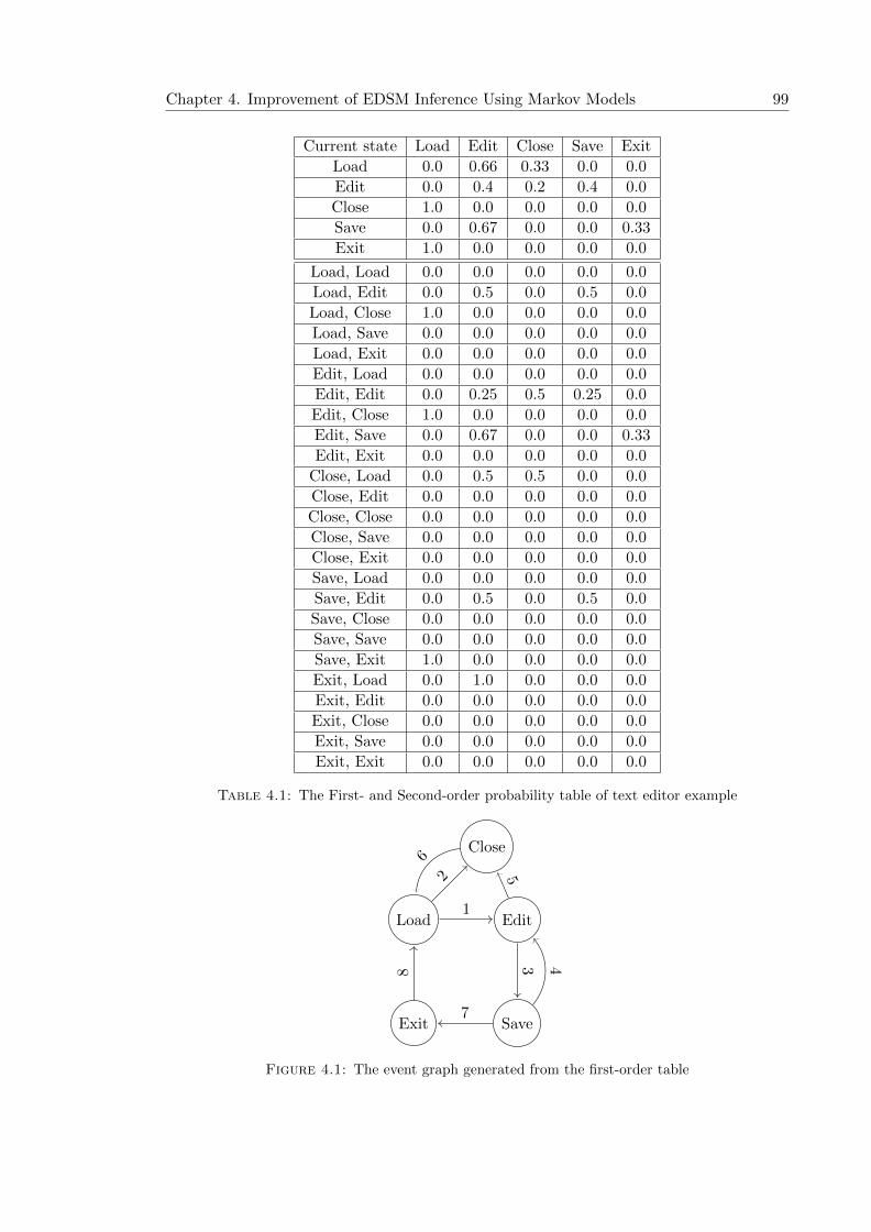
Chapter 4. Improvement of EDSM Inference Using Markov Models 99
Current state Load Edit Close Save Exit
Load 0.0 0.66 0.33 0.0 0.0
Edit 0.0 0.4 0.2 0.4 0.0
Close 1.0 0.0 0.0 0.0 0.0
Save 0.0 0.67 0.0 0.0 0.33
Exit 1.0 0.0 0.0 0.0 0.0
Load, Load 0.0 0.0 0.0 0.0 0.0
Load, Edit 0.0 0.5 0.0 0.5 0.0
Load, Close 1.0 0.0 0.0 0.0 0.0
Load, Save 0.0 0.0 0.0 0.0 0.0
Load, Exit 0.0 0.0 0.0 0.0 0.0
Edit, Load 0.0 0.0 0.0 0.0 0.0
Edit, Edit 0.0 0.25 0.5 0.25 0.0
Edit, Close 1.0 0.0 0.0 0.0 0.0
Edit, Save 0.0 0.67 0.0 0.0 0.33
Edit, Exit 0.0 0.0 0.0 0.0 0.0
Close, Load 0.0 0.5 0.5 0.0 0.0
Close, Edit 0.0 0.0 0.0 0.0 0.0
Close, Close 0.0 0.0 0.0 0.0 0.0
Close, Save 0.0 0.0 0.0 0.0 0.0
Close, Exit 0.0 0.0 0.0 0.0 0.0
Save, Load 0.0 0.0 0.0 0.0 0.0
Save, Edit 0.0 0.5 0.0 0.5 0.0
Save, Close 0.0 0.0 0.0 0.0 0.0
Save, Save 0.0 0.0 0.0 0.0 0.0
Save, Exit 1.0 0.0 0.0 0.0 0.0
Exit, Load 0.0 1.0 0.0 0.0 0.0
Exit, Edit 0.0 0.0 0.0 0.0 0.0
Exit, Close 0.0 0.0 0.0 0.0 0.0
Exit, Save 0.0 0.0 0.0 0.0 0.0
Exit, Exit 0.0 0.0 0.0 0.0 0.0
Table 4.1: The First- and Second-order probability table of text editor example
Load Edit
SaveExit
Close
1
2
35
4
7
68
Figure 4.1: The event graph generated from the first-order table

Chapter 4. Improvement of EDSM Inference Using Markov Models 100
4.3 The Proposed Markov Models
In this section the proposed Markov model (ML) is described. It relies on predicting one
element of alphabet σ ∈ Σ depending on the previous k elements of alphabet.
As described in the previous section, Cook and Wolf [49] mapped entries of the Markov
table into probabilities reflecting how frequent short event sequences of a specific length
appeared in the training data. They [49] used a cut-off threshold to avoid noise in training
data to identify the most probable event sequences.
In this thesis, the assumption is that training data is very sparse, and it is hard to use a
non-zero threshold such as that used by Cook and Wolf [49] to identify the most probable
sequences since there is no noise in training data. Moreover, sequence of events with
low frequencies cannot be ignored because they can be indicators of valid predictions.
Therefore, predictions are based on the presence or absence of specific sequences rather
than the number of times they are observed.
4.3.1 Building the Markov Table
This section describes the way of training Markov model. It begins by creating the event-
sequence table. In general, the event-sequence table is constructed in the same way as
proposed by Cook and Wolf [49]. However, the entries in the event-sequence table are
boolean values to denote whether an event is permitted or prohibited to follow sequences.
The process of building the Markov table (MT ) initially requires a sample of positive and
possibly few negative traces similar to those that feed into any state-merging technique.
Each trace is a sequence of alphabet elements representing a sequence of events. After
that, the construction of the MT is performed by choosing a prefix length k and recording
elements of an alphabet (events) following a subsequence of length k in any of the traces
in the training data. Hence, k can be seen as the order of the Markov model.
Given a training sequence σ1, σ2, . . . , σn, one looks at subsequences σi, σi+1, . . . , σi+k−1, σi+k
and records them as pairs of two elements. The first part in the pair is called the prefix
sequence of the current subsequence of length k over Σ∗. The second part is a suffix which
is an element of alphabet σ ∈ Σ.

Chapter 4. Improvement of EDSM Inference Using Markov Models 101
Current state Load Edit Close Save Exit
Load - pos - pos -
Edit - pos - pos -
Close pos Neg - - -
Save - pos - - pos
Exit pos - - - -
Load, Load - - - - -
Load, Edit - pos - pos -
Load, Close pos - - - -
Load, Save - - - - -
Load, Exit - - - - -
Edit, Load - - - - -
Edit, Edit - - - - -
Edit, Close pos - - - -
Edit, Save - pos - - pos
Edit, Exit - - - - -
Close, Load - pos pos - -
Close, Edit - - - - -
Close, Close - - - - -
Close, Save - - - - -
Close, Exit - - - - -
Save, Load - - - - -
Save, Edit - pos - pos -
Save, Close - - - - -
Save, Save - - - - -
Save, Exit pos - - - -
Exit, Load - pos - - -
Exit, Edit - - - - -
Exit, Close - - - - -
Exit, Save - - - - -
Exit, Exit - - - - -
Table 4.2: The First- and Second-order event-sequence table of text editor example
The next step is to record a pair (〈σi, σi+1, . . . , σi+k−1〉, σi+k) as a positive if σi+k is a
permitted event to follow the prefix sequence 〈σi, σi+1, . . . , σi+k−1〉, a negative if it is not,
and a failure, if for the same prefix sequence, both a positive and a negative occurrence
of the same event were observed. Since the focus is on inference of LTSs which recog-
nise prefix-closed languages, the only case where σi+k is a negative is if it is at the end
of a trace from negative traces S−. For the purpose of predictions, failure entries are
ignored. Definition 4.1 defined the MT table in the proposed ML
Definition 4.1. Let Markov = {Pos,Neg, Fail} be possible entries of Markov table

Chapter 4. Improvement of EDSM Inference Using Markov Models 102
MT. A MT is mapping MT : Σk × Σ 7→ Markov. The domain of the MT func-
tion is given by dom(MT) = Σk × Σ. The outcome from the Markov table for a pair
(〈σi, σi+1, . . . , σi+k−1〉, σi+k) ∈ dom (MT) is given by MT (〈σi, σi+1, . . . , σi+k−1〉, σi+k).
A Markov prediction is a label (an element of alphabet) that the trained Markov model
suggested either to follow or not to follow a sequence σ ∈ ΣK . In terms of execution
traces, a prediction is a function or a method name that is either predicted to be called
after invoking sequences of methods, or prohibited to after them. From Definition 4.1,
we say that a label (an element of alphabet) σi+k is predicted as permitted to follow
〈σi, σi+1, . . . , σi+k−1〉 if MT (〈σi, σi+1, . . . , σi+k−1〉, σi+k) = Pos. On the other hand, a la-
bel (an element of alphabet) σi+k is predicted as prohibited to follow 〈σi, σi+1, . . . , σi+k−1〉
if MT (〈σi, σi+1, . . . , σi+k−1〉, σi+k) = Neg.
Algorithm 9 describes the process of building the Markov table from both positive and
negative traces. The obtainSubsequence is responsible for splitting a sequence into subse-
quences of elements of length k + 1. For example, for a trace σ1, σ2, σ3, σ3, σ5, consider
that k = 2 and i = 1; the σ1, σ2, σ3 subsequence is returned. The process of constructing
the Markov table begins with the positive sequences before the negative ones. The process
of building the Markov table is terminated when all traces have been processed. It is
important to highlight that ⊕ denote the override process on table entries.
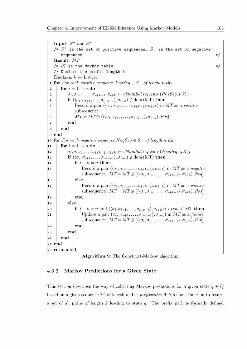
Chapter 4. Improvement of EDSM Inference Using Markov Models 103
Input: S+ and S−
/* S+ is the set of positive sequences, S− is the set of negative
sequences */
Result: MT/* MT is the Markov table */
// Declare the prefix length kDeclare: k ← Integer
1 for For each positive sequence PosSeq ∈ S+ of length n do2 for i = 1 · · ·n do3 σi, σi+1, . . . , σi+k−1, σi+k ← obtainSubsequence (PosSeq, i, k);4 if (〈σi, σi+1, . . . , σi+k−1〉, σi+k) /∈ dom (MT) then5 Record a pair (〈σi, σi+1, . . . , σi+k−1〉, σi+k) in MT as a positive
subsequence.6 MT = MT⊕
((〈σi, σi+1, . . . , σi+k−1〉, σi+k),Pos
)7 end
8 end
9 end10 for For each negative sequence NeqSeq ∈ S− of length n do11 for i = 1→ n do12 σi, σi+1, . . . , σi+k−1, σi+k ← obtainSubsequence (NeqSeq, i,K);13 if (〈σi, σi+1, . . . , σi+k−1〉, σi+k) /∈ dom (MT) then14 if i+ k = n then15 Record a pair (〈σi, σi+1, . . . , σi+k−1〉, σi+k) in MT as a negative
subsequence. MT = MT⊕((〈σi, σi+1, . . . , σi+k−1〉, σi+k),Neg
)16 else17 Record a pair (〈σi, σi+1, . . . , σi+k−1〉, σi+k) in MT as a positive
subsequence. MT = MT⊕((〈σi, σi+1, . . . , σi+k−1〉, σi+k),Pos
)18 end
19 else20 if i+ k = n and (〈σi, σi+1, . . . , σi+k−1〉, σi+k) 7→ true ∈ MT then21 Update a pair (〈σi, σi+1, . . . , σi+k−1〉, σi+k) in MT as a failure
subsequence. MT = MT⊕((〈σi, σi+1, . . . , σi+k−1〉, σi+k),Fail
)22 end
23 end
24 end
25 end26 return MT
Algorithm 9: The Construct-Markov algorithm
4.3.2 Markov Predictions for a Given State
This section describes the way of collecting Markov predictions for a given state q ∈ Q
based on a given sequence Σk of length k. Let prefixpaths (A, k, q) be a function to return
a set of all paths of length k leading to state q. The prefix path is formally defined

Chapter 4. Improvement of EDSM Inference Using Markov Models 104
in Definition 4.2. It differs from the prefix sequence that takes a path from the initial state
to q.
Definition 4.2. Given a state q ∈ Q and LTS A. The set of prefix paths that lead to q
is given by: prefixpaths (A, k, q) = {σ ∈ Σk | ∃q′ ∈ Q. δ(q′, σ) = q}
Definition 4.3. Given a sequence of length k (prefix path), denoted by pr over Σ and
the Markov table MT. The set of permitted predictions for a given q after pr is given by:
MLpermitted (q, pr) = {σ ∈ Σ | MT (pr, σ) = pos, (pr, σ) ∈ dom(MT)}
Definition 4.4. Given a sequence of length k (prefix path), denoted by pr over Σ and
the Markov table MT. The set of prohibited predictions for a given q after pr is given by:
MLprohibited (q, pr) = {σ ∈ Σ | MT (pr, σ) = Neg, (pr, σ) ∈ dom(MT)}
4.3.3 The Precision and Recall of the Markov Model
This section describes how to check the correctness of the trained Markov model with
respect to the reference LTS model in terms of their outgoing transitions. It begins with
definitions related to obtaining Markov predictions for a given state q ∈ Q.
4.3.4 Definitions of Precision and Recall for Markov Models
For computing the precision and recall purposes, Definition 4.5 suggested that an element
of alphabet σ is returned as permitted to follow the given state q on the following condition.
If σ is predicted as permitted to follow q for at least one prefix path and there does not
exist another prefix path suggesting that σ is prohibited to follow q.
Definition 4.5. Given an element of alphabet σ ∈ Σ, a state q ∈ Q, Markov table (MT),
prefix length k and LTS A. We say that σ is returned as permitted prediction if:
1. (∃pr ∈ prefixpaths (A, k, q), σ ∈ MLpermitted (q, pr)) ∧ (@pr′ ∈ prefixpaths (A, k, q), σ ∈
MLprohibited (q, pr′))
Definition 4.6 stated that an element of alphabet σ is returned as prohibited to follow the
given state q on the following condition. If σ is predicted as prohibited to follow q for
at least one prefix path and there does not exist another prefix path suggesting that σ is
permitted to follow q.

Chapter 4. Improvement of EDSM Inference Using Markov Models 105
Definition 4.6. Given an element of alphabet σ ∈ Σ, a state q ∈ Q, Markov table (MT),
prefix length k and LTS A. We say that σ is returned as prohibited prediction:
1. (∃pr ∈ prefixpaths (A, k, q), σ ∈ MLprohibited (q, pr)) ∧ (@pr′ ∈ prefixpaths (A, k, q), σ ∈
MLpermitted (q, pr′))
The precision and recall metric is computed with respect to the outgoing transitions of
reference LTSs. It is important to determine which of the returned predictions are rele-
vant. Definition 4.7 shows how accurate (relevant) the returned predictions are with respect
to the outgoing transitions in the reference LTS. A returned prediction σ is said to be rel-
evant in two cases. First, if a is predicted as permitted to follow a given state q and there
is a transition labelled with σ lead to q′ ∈ Q. Second, if a is predicted as prohibited to
follow a given state q and there does not exist a transition labelled with σ lead to q′ /∈ Q.
It is worth-mentioning that all states in an LTS are accepted as described in Chapter 2
Definition 4.7. Given a state q ∈ Q and LTS A. A returned Markov prediction from the
q is relevant if any of the following conditions are satisfied.
1. A returned prediction satisfying conditions in Definition 4.5, which element of alpha-
bet σ is said relevant as permitted from the given state q in the reference LTS if:
∃q′ ∈ Q such that δ(q, σ) = q′ and MT (pr, σ) = Pos.
2. A returned prediction satisfying conditions in Definition 4.6, which element of al-
phabet σ is said relevant as prohibited from the given state q in the reference LTS
if: δ(q, σ) = ∅ and MT (pr, σ) = Neg.
It is important to highlight that the returned and relevant predictions that are defined in
this section are used to compute the precision and recall scores in the following sections.
4.3.5 Markov Precision and Recall
This section introduces the precision and recall metrics that are computed to measure the
correctness of Markov model. Therefore, predictions made by the trained Markov models
are measured against the transitions in the target reference graph. The correctness of
Markov models are measured using the precision and recall metrics that are designed to

Chapter 4. Improvement of EDSM Inference Using Markov Models 106
cope with predictions. This is inspired by the use of precision and recall metrics in the
information retrieval context.
In an information retrieval context, the precision is defined as the proportion of retrieved
documents that are relevant [99]. The precision of the Markov model can be defined as
the proportion of returned predictions that are relevant (see Definition 4.7). It is used to
evaluate how accurate the returned predictions by the Markov model are.
The precision summarizes the exactness of the predictions. A high precision score means
that the trained Markov model captures the dependencies between events in the traces
well.
Precision =| returned predictions | ∩ | relevant predictions |
| returned predictions |(4.1)
Additionally, in an information retrieval context, the recall is defined as the proportion
of relevant documents that are returned [99]. The recall of the trained Markov models is
defined as the proportion of labels of outgoing transitions in the reference graph that are
predicted correctly. It is introduced to measure how complete labels of the outgoing tran-
sitions in the reference graph are predicted correctly. Furthermore, the recall summarizes
the completeness of predictions.
Recall =| returned predictions | ∩ | relevant predictions |
| relevant labels|(4.2)
Example 4.2. Consider the reference LTS of the text editor shown in Figure 4.2. Table 4.3
illustrates theMT that was built from the following positive traces: S+ = {〈Load,Edit,Close,
Load,Edit,Edit,Edit〉, 〈Load,Edit,Close,Load,Close,Load,Edit〉, 〈Load,Close,Load,Close〉}
where k = 1. Label Save is not predicted from the D state since the trained Markov model
did not observe the subsequence 〈Edit, Save〉. Moreover, label Exit is not predicted from
A, B, and D states. Other transitions are predicted correctly. The precision is given by
5/5 = 1, and the recall is given by 5/9 = 0.55. In this example, no extra wrong predictions
are made from each state. However, four relevant labels of outgoing transition are not
predicted.
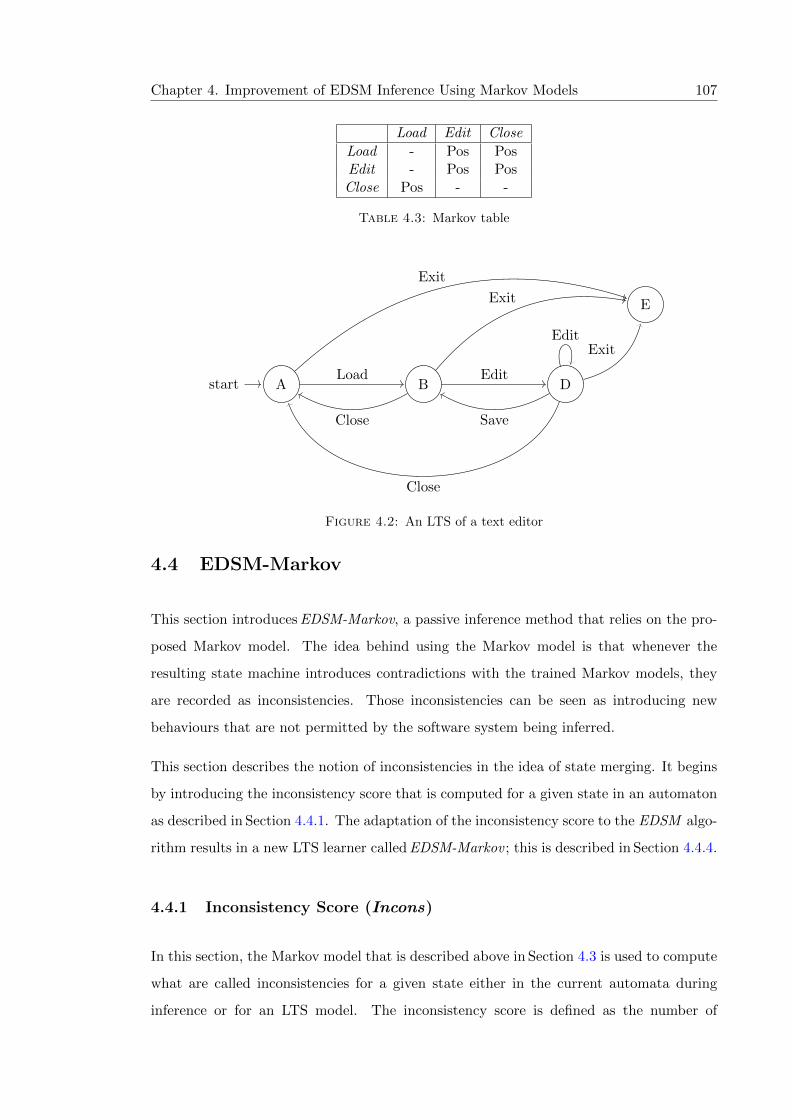
Chapter 4. Improvement of EDSM Inference Using Markov Models 107
Load Edit Close
Load - Pos PosEdit - Pos PosClose Pos - -
Table 4.3: Markov table
Astart B D
E
Load
Exit
Exit
Close
Edit
Edit
Close
Save
Exit
Figure 4.2: An LTS of a text editor
4.4 EDSM-Markov
This section introduces EDSM-Markov, a passive inference method that relies on the pro-
posed Markov model. The idea behind using the Markov model is that whenever the
resulting state machine introduces contradictions with the trained Markov models, they
are recorded as inconsistencies. Those inconsistencies can be seen as introducing new
behaviours that are not permitted by the software system being inferred.
This section describes the notion of inconsistencies in the idea of state merging. It begins
by introducing the inconsistency score that is computed for a given state in an automaton
as described in Section 4.4.1. The adaptation of the inconsistency score to the EDSM algo-
rithm results in a new LTS learner called EDSM-Markov ; this is described in Section 4.4.4.
4.4.1 Inconsistency Score (Incons)
In this section, the Markov model that is described above in Section 4.3 is used to compute
what are called inconsistencies for a given state either in the current automata during
inference or for an LTS model. The inconsistency score is defined as the number of

Chapter 4. Improvement of EDSM Inference Using Markov Models 108
contradictions between the existing labels of the outgoing transitions against corresponding
predictions, for a given state or for all states in an LTS.
4.4.1.1 Inconsistency Score for a Specific State
In this section, the process of finding and counting the inconsistency score for a given
state is described. The inconsistency score for a given state is computed with respect
to its outgoing transitions. It begins by collecting the set of prefix paths for a given a
state prefixpaths (A, k, q) as described in Definition 4.2. Then, a set of labels of outgoing
transitions are obtained, denoted Σoutq and defined in Definition 2.3.
A label of an outgoing transition σ ∈ Σoutq is said to be consistent if there is a match be-
tween the outgoing transition and the corresponding prediction as defined in Definition 4.8.
Definition 4.8. Given a state q ∈ Q, prefix length k, automaton A, a prefix path pr ∈
prefixpaths (A, k, q), a label of outgoing transition σ, and the trained Markov model MT.
An element of alphabet σ is said to be consistent based on Markov predictions for a prefix
paths pr if:
1. (∃q′ ∈ F+. δ(q, σ) = q′ ∧ σ ∈ MLpermitted (q, pr)) ∨ (∃q′′ ∈ F−. δ(q, σ) = q′′ ∧ σ ∈
MLprohibited (q, pr))
From Definition 4.8, a label of outgoing transition σ ∈ Σoutq is said to be consistent with
Markov predictions in two cases. First, if there is a transition labelled with σ that leads to
an accepting state from a state q and the σ is predicted as permitted to follow pr. The first
case if the provided automaton is LTS or PTA. Second, if σ is predicted by the Markov
model as prohibited after pr and there is an outgoing transition labelled with σ leaving a
state q leading to a rejecting state q′ ∈ F−. The second case is included alongside the first
case if the learner infers PLTS from positive and negative traces. Otherwise, σ is said to
be inconsistent for the current prefix path pr ∈ prefixpaths (A, k, q).
Algorithm 10 summarized the process of computationvof the inconsistency score for a
given state q ∈ Q in the current automaton A, and this score is denoted by (Inconsq).
It begins by collecting a set of all prefix paths of length k leading to state q. The
prefixpaths(A, q, k) function in Algorithm 10 returns all prefix paths. For example, for

Chapter 4. Improvement of EDSM Inference Using Markov Models 109
the automaton A and state B that is illustrated in Figure 4.3, the set of prefix path of
length 1 is prefixpaths(A,B, 1) = {〈Load〉, 〈Close〉} and the set of prefix path of length 2
contains prefixpaths(A,B, 2) = {〈Load,Close〉, 〈Close,
Close〉}.
Ostart B
C
G
E
H I
F
ZLoad
Edit
Load
CloseEdi
t
Save
Save Close
Close
Figure 4.3: Example of computing Inconsq
Input: q and k/* S+ is the current state, k is the prefix length k */
Result: Inconsq// Inconsq is the number of inconsistencies
1 Inconsq ← 0;2 for pr ∈ prefixpaths(A, q, k) of length k do3 for σ ∈ Σout
q do
4 if checkConsistencies (pr, σ,MT) is false then5 incons← incons ∪ (pr, σ);6 else7 cons← cons ∪ (pr, σ);8 end
9 end
10 end11 return Inconsq ← |incons|
Algorithm 10: The computation of inconsistency for a given state q
The second step during the computation of the Inconsq score is to check the consistency of
each element in Σoutq against Markov predictions. The aim is to find inconsistencies (con-
tradictions) between the outgoing transitions and the corresponding predictions. Given a
state q, the computation of the Inconsq score is achieved by iterating through the set of
prefix path leading to q, and checking the consistency of an element of alphabet σ ∈ Σoutq
for the current pr. It classifies each given prefix path and each label in Σoutq into the incon-
sistent (incons) and consistent (cons) sets as shown in Table 4.4. If a label of an outgoing
transition σ ∈ Σoutq is consistent with respect to a prefix path pr ∈ prefixpaths(A, q, k),
Chapter 4. Improvement of EDSM Inference Using Markov Models 110
then the pair (pr, σ) is added to the cons set. Otherwise, it is added to the incons set. It is
important to highlight that the consistency (matching) of the label of outgoing transition
σ with predictions is determined as described in the previous section (see Definition 4.8).
The Inconsq score is the number of pairs that are added to the incons set after the classi-
fication process.
pr ∈
PrefixPaths(A,q,k)
Markov predictions
σ ∈ MLpermitted(pr) σ ∈ MLprohibitted(pr) (pr, σ) /∈ dom(MT)
σ ∈ Σoutq | q′ = δ(q, σ), q′ ∈ F+ cons incons incons
σ ∈ Σoutq | q′ = δ(q, σ), q′ ∈ F− incons cons incons
Table 4.4: Classification of inconsistency
Load Edit Save Close
Load, Load - - - -Load, Edit - Pos Pos -Load, Save - - - -Load, Close Pos - - -Edit, Load - - - -Edit, Edit - - Pos -Edit, Save - - - PosEdit, Close - - - -Save, Load - - - -Save, Edit - - - -Save, Save - - - -Save, Close - - - -Close, Load - - - -Close, Edit - - - -Close, Save - - - -Close, Close - - - -
Table 4.5: The Markov Table where k = 2
Example 4.3. Let us again consider the automaton shown in Figure 4.3, and the MT illus-
trated in Table 4.5 where k = 2. The MT is built from the following positive traces: S+ =
{〈Load,Edit,Edit,Save,Close〉, 〈Load,Edit,Save,Close〉, 〈Load,Close,Load〉}. The set of
labels of outgoing transitions of state B (ΣoutB ) contains the following labels: {Load,Edit,Close}.
The prefixpaths (A,B, 2) function returns the following prefix paths: {〈Load,Close〉, 〈Close,
Close〉}. The next step is to check consistency for each label in the ΣoutB set against
Markov predictions for each prefix path in prefixpaths (A,B, 2). For instance, the Load
label is predicted as permitted to follow 〈Load,Close〉 based on the Markov table that

Chapter 4. Improvement of EDSM Inference Using Markov Models 111
is illustrated in Table 4.5. Thus, the Load label is considered consistent since there is an
outgoing transition that leads to the accepting state labelled with Z. However, the Load
label is not predicted after the prefix path 〈Close, Close〉, and this is considered as in-
consistency. Table 4.6 shows the inconsistency classification for each label of the outgoing
transitions for the B state where the prefix path is 〈Load,Close〉.
〈Load,Close〉 ∈
collectPrefixPaths(A,q,k)
Markov Table (MT)
σ ∈ MLpermitted(〈Load,Close〉) σ ∈ MLprohibitted(〈Load,Close〉) (〈Load,Close〉, σ) /∈ dom(MT)
Load ∈ ΣoutB | δ(B, σ) = K ∈ F+ cons - -
Edit ∈ ΣoutB | δ(B, σ) = C ∈ F+ - - incons
Close ∈ ΣoutB | δ(B, σ) = B ∈ F+ - - incons
Table 4.6: Classification of inconsistency for the prefix path 〈Load,Close〉 and state B
4.4.1.2 Inconsistency Score for an Automaton
The computation of Incons for an automaton is described formally in Definition 4.9, where
Incons(A,MT, q) is the function that returns the inconsistency score for a given state and
it is computed as described in the previous section.
Definition 4.9.
Incons(A,MT) =∑q∈QA
Incons(A,MT, q)
4.4.2 Inconsistency Heuristic for State Merging
This section introduced the idea of incorporating the computation of inconsistency during
the state-merging process. It is known that the EDSM heuristic is concerned with the
amount of evidence suggesting that the pair of states are equivalent. Instead of focusing
on computing the agreement evidence between a pair of states, one would compute the
disagreement between them to measure how likely it is that the states are different. Since
negative sequences are usually missing or not sufficient to prevent over-generalizing during
the state-merging process, the computation of Incons(A,MT, q) described in the previous
section can be used to determine whether a specific transition matches predictions or not
from a particular state. In other words, inconsistencies that may appear as a result of
merging states imply that the current hypothesis (LTS) accepts sequences of elements of
length k + 1 where the Markov model does not, and vice versa.

Chapter 4. Improvement of EDSM Inference Using Markov Models 112
This section presents an inconsistency score that is computed for a given pair of states
during the state-merging process and this is denoted by Im. The Im score is comput-
ing by taking the difference of two inconsistency scores. The first inconsistency is com-
puted for a merged automaton and the second one for the automaton before merging the
states. Given two states q and q′ that are chosen for merging, the inconsistency Im score
is obtained by first computing the inconsistency of the current automaton, denoted by
Incons(A,MT). Where q and q′ of A are merged, a new inconsistency of the merged
automaton Incons(merge(A, q, q′),MT) is computed. The inconsistency score for a given
pair of states Im is obtained as follows:
Im = Incons(merge(A, q, q′),MT)− Incons(A,MT) (4.3)
The intention behind computing Im for a given pair of states is to determine how many
inconsistencies resulted from merging the states. It is important to highlight the fact
that the merge(A, q, q′) function in Equation 4.3 is the merging procedure as described
in Section 3.1.4. Moreover, the computation of the inconsistency for the current automaton
Incons(A,MT) is necessary to isolate the inconsistencies observed as a result of previous
mergers from those detected from computing the current merger of states. Example 4.4
and 4.5 below illustrates the way of computing the Im score.
Example 4.4. Consider a PTA of the text editor example that is shown in Figure 4.4
and assume that states B and C are chosen to be merged by a learner. In this way, the
process of computation of Im includes building the Markov table and getting predictions
as described in Section 4.3. The merging process results in an LTS as shown in Figure 4.5
where a transition that is labelled with close from BCG state is not predicted after the
following prefix path: 〈Edit〉. This is considered as an inconsistency of merging B and C
states. In addition, another inconsistency that occurred as a consequence of merging B
state with C is that the outgoing transition labelled with Save leaving BCG state is not
predicted by MT after the following prefix sequence: 〈Load〉. Hence, merging of B and C
states resulted in an Im score of two.
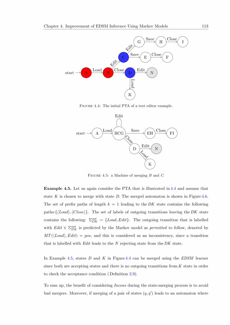
Chapter 4. Improvement of EDSM Inference Using Markov Models 113
Astart B
C
D
G
E
H I
F
N
K
Load
Edit
Close
Edit
Save
Save Close
Close
Edit
Load
Figure 4.4: The initial PTA of a text editor example.
Astart BCG
D
EH FI
N
K
Load
Edit
Close
Save Close
Edit
Load
Figure 4.5: a Machine of merging B and C.
Example 4.5. Let us again consider the PTA that is illustrated in 4.4 and assume that
state K is chosen to merge with state D. The merged automaton is shown in Figure 4.6.
The set of prefix paths of length k = 1 leading to the DK state contains the following
paths:{〈Load〉, 〈Close〉}. The set of labels of outgoing transitions leaving the DK state
contains the following: ΣoutDK = {Load,Edit}. The outgoing transition that is labelled
with Edit ∈ ΣoutDK is predicted by the Markov model as permitted to follow, denoted by
MT (〈Load〉, Edit) = pos, and this is considered as an inconsistency, since a transition
that is labelled with Edit leads to the N rejecting state from the DK state.
In Example 4.5, states D and K in Figure 4.4 can be merged using the EDSM learner
since both are accepting states and there is no outgoing transitions from K state in order
to check the acceptance condition ( Definition 2.9).
To sum up, the benefit of considering Incons during the state-merging process is to avoid
bad mergers. Moreover, if merging of a pair of states (q, q′) leads to an automaton where

Chapter 4. Improvement of EDSM Inference Using Markov Models 114
Astart B
C
DK
G
E
H I
F
N
Load
Edit
Close
Edit
Save
Save Close
Close
Edit
Load
Figure 4.6: a Machine of merging D and K.
one or more outgoing transitions from q, q′ are not predicted by the trained Markov model,
this is not considered good if there is another possible pair of states such that all outgoing
transitions from the pair match predictions. In other words, merging a pair of states
among other possible pairs is considered to be a good decision if the merger leads to an
automaton with the maximum matching of outgoing transitions with the predicted ones.
The next section describes the way of incorporating the Incons value for each merger of
states with the EDSM heuristic in order to infer good LTSs.
4.4.3 EDSM-Inconsistency Heuristic
The proposed EDSM-inconsistency heuristic is introduced to demonstrate that the EDSM
algorithm can benefit from the computation of inconsistencies. The purpose of the EDSM-
inconsistency heuristic is to prevent merging of inconsistent pairs of states and to rank
them using both EDSM scores and inconsistencies. A pair with a high EDSM score
and low inconsistency score is considered to be the most likely pair to be merged. The
presented heuristic approach is to compute an EDSM score of a pair of states and subtract
the inconsistency score Im from it.
The computation of scores of pairs following the EDSM-inconsistency heuristic is described
in Definition 4.10.
Definition 4.10.
IScore(A, q, q′,MT) = edsmScore (A, q, q′)−(Incons(merge(A, q, q′),MT)− Incons(A,MT)
)

Chapter 4. Improvement of EDSM Inference Using Markov Models 115
Definition 4.11.
IScore(A, q, q′,MT) = edsmScore (A, q, q′)− Im
The score of the EDSM-inconsistency can be simply obtained via edsmScore(A, q, q′)−Im.
For example, consider a merged automaton shown in Figure 4.5 resulting from merging
B,C states. In this case, the EDSM score is 4 since the number of states in the automaton
has dropped from 11 to 7. The inconsistency score of the automaton before merging states
denoted Incons(A,MT) is 0 since the Markov model is trained from the original PTA and
no mergers have been performed yet. After the merging of B and C, the inconsistency
score of merged graph Incons(merge(A, q, q′)) is 2 since the outgoing transition labelled
with Save is not predicted after the prefix path 〈Load〉 and the same for the outgoing
transition labelled with Close and the prefix path 〈Edit〉. The final inconsistency score
Im is 2. So, the EDSM-inconsistency score is 2 in this example, because it is given by
subtracting the Im score from EDSM.
Definition 4.12.
IScore(A, q, q′,MT) = edsmScore (A, q, q′)− (Im× Incon)
We ran an experiment to vary the Im score by introducing the multiplier Incon. Hence,
the IScore(A, q, q′,MT) score that is introduced in Definition 4.11 is rewritten as shown
in Definition 4.12 The idea behind this experiment is to study the influence of the Im score
compared to the EDSM score, justifying why those two heuristics are combined.
In the conducted experiment, random LTSs were generated using the Forest Fire algorithm
that is described in Section 2.6. The number of states ranged between 10 and 40 in steps
of 10. Fifteen LTSs were generated for each selected number of states. Hence, the total
number of random LTSs is 4 steps ∗ 15 = 60 LTSs. For each LTS, 5 sets of training data
were generated, bringing the number of LTSs learnt per experiment to 300. In addition,
the randomly generated LTSs were connected, and had an alphabet size two times the
number of states. Moreover, the influence of Incon were studied with different numbers
of traces where it ranged from 1 to 7 traces, incrementing by 2. The length of traces is
given by |Q| ∗ |Σ| (= 2 ∗ |Q|2). This figure is loosely motivated by the size of a transition

Chapter 4. Improvement of EDSM Inference Using Markov Models 116
cover set, which is the number of sequences to reach every state of an LTS and attempt
every input in it.
The boxplots of the BCR scores obtained by EDSM-Markov for all various inconsistency
multiplier Incon considered are illustrated in Figure 4.7. The BCR scores attained by
the EDSM-Markov learner are high when Incon = 1 compared to other settings of Incon.
However, it is clear that the performance of EDSM-Markov learner tend to be worse when
Incon > 1. The reason behind this is that the following expression (Im × Incon) will
exceed EDSM scores and forcing the EDSM-Markov learner to block mergers. Hence, the
inferred models will be under-generalized.
1 3
5 70.4
0.5
0.6
0.7
0.8
0.9
1.0
0.4
0.5
0.6
0.7
0.8
0.9
1.0
Incon=0.5 Incon=1.0 Incon=2.0 Incon=3.0 Incon=4.0 Incon=0.5 Incon=1.0 Incon=2.0 Incon=3.0 Incon=4.0Inconsistency Muliplier
BC
R s
core
EDSM−Markov
Trace Number
Figure 4.7: BCR scores obtained by EDSM-Markov for different inconsistency multiplierIncon
The boxplots of the structural-similarity scores obtained by EDSM-Markov for different
settings of Incon are depicted in Figure 4.8. With Incon = 1, the structural-similarity
scores achieved by EDSM-Markov are the highest compared to other settings of Incon.
As can be seen in Figure 4.8, the structural-similarity scores attained by EDSM-Markov
are affected by different settings of Incon. The structural-similarity scores are decreased
dramatically when Incon > 1.0 where the inferred models are under-generalized.
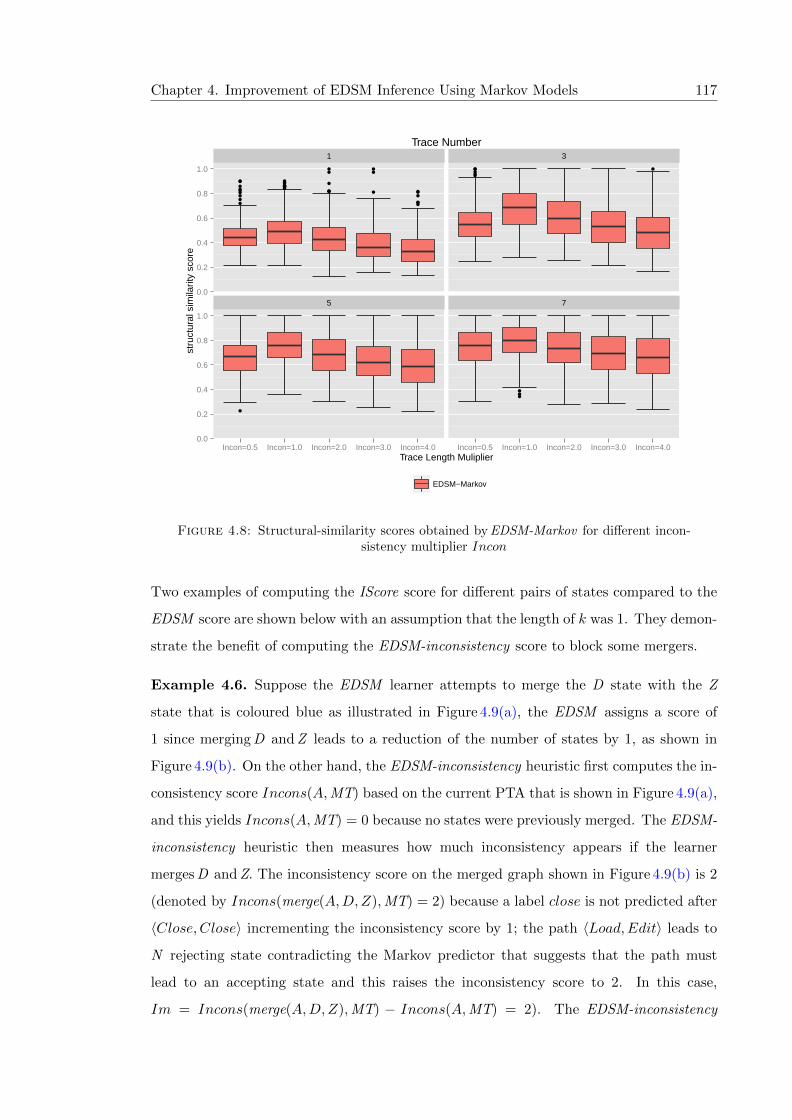
Chapter 4. Improvement of EDSM Inference Using Markov Models 117
1 3
5 70.0
0.2
0.4
0.6
0.8
1.0
0.0
0.2
0.4
0.6
0.8
1.0
Incon=0.5 Incon=1.0 Incon=2.0 Incon=3.0 Incon=4.0 Incon=0.5 Incon=1.0 Incon=2.0 Incon=3.0 Incon=4.0Trace Length Muliplier
stru
ctur
al s
imila
rity
scor
e
EDSM−Markov
Trace Number
Figure 4.8: Structural-similarity scores obtained by EDSM-Markov for different incon-sistency multiplier Incon
Two examples of computing the IScore score for different pairs of states compared to the
EDSM score are shown below with an assumption that the length of k was 1. They demon-
strate the benefit of computing the EDSM-inconsistency score to block some mergers.
Example 4.6. Suppose the EDSM learner attempts to merge the D state with the Z
state that is coloured blue as illustrated in Figure 4.9(a), the EDSM assigns a score of
1 since merging D and Z leads to a reduction of the number of states by 1, as shown in
Figure 4.9(b). On the other hand, the EDSM-inconsistency heuristic first computes the in-
consistency score Incons(A,MT) based on the current PTA that is shown in Figure 4.9(a),
and this yields Incons(A,MT) = 0 because no states were previously merged. The EDSM-
inconsistency heuristic then measures how much inconsistency appears if the learner
merges D and Z. The inconsistency score on the merged graph shown in Figure 4.9(b) is 2
(denoted by Incons(merge(A,D,Z),MT) = 2) because a label close is not predicted after
〈Close, Close〉 incrementing the inconsistency score by 1; the path 〈Load,Edit〉 leads to
N rejecting state contradicting the Markov predictor that suggests that the path must
lead to an accepting state and this raises the inconsistency score to 2. In this case,
Im = Incons(merge(A,D,Z),MT) − Incons(A,MT) = 2). The EDSM-inconsistency
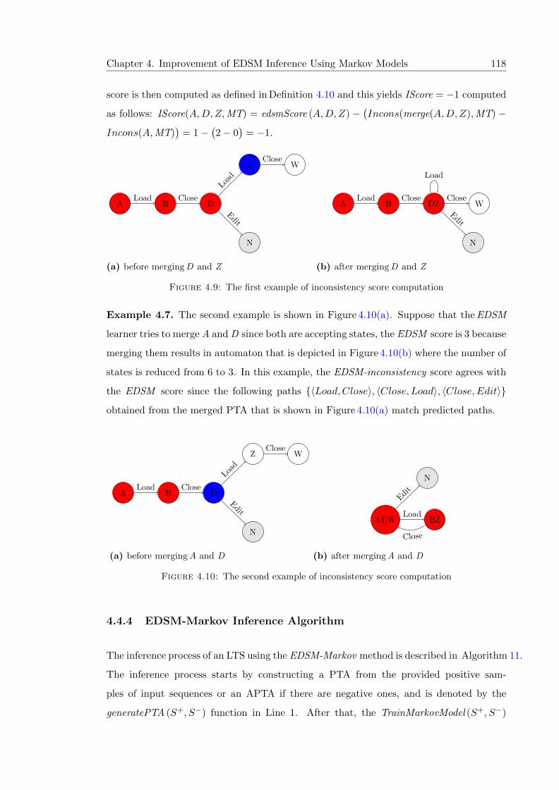
Chapter 4. Improvement of EDSM Inference Using Markov Models 118
score is then computed as defined in Definition 4.10 and this yields IScore = −1 computed
as follows: IScore(A,D,Z,MT) = edsmScore (A,D,Z) −(Incons(merge(A,D,Z),MT) −
Incons(A,MT))
= 1−(2− 0
)= −1.
A B D
N
Z W
Load Close
Edit
Load
Close
(a) before merging D and Z
A B DZ
N
WLoad Close
Edit
Load
Close
(b) after merging D and Z
Figure 4.9: The first example of inconsistency score computation
Example 4.7. The second example is shown in Figure 4.10(a). Suppose that the EDSM
learner tries to merge A and D since both are accepting states, the EDSM score is 3 because
merging them results in automaton that is depicted in Figure 4.10(b) where the number of
states is reduced from 6 to 3. In this example, the EDSM-inconsistency score agrees with
the EDSM score since the following paths {〈Load,Close〉, 〈Close, Load〉, 〈Close,Edit〉}
obtained from the merged PTA that is shown in Figure 4.10(a) match predicted paths.
A B D
N
Z W
Load Close
Edit
Load
Close
(a) before merging A and D
ADW BZ
N
Load
Edit
Close
(b) after merging A and D
Figure 4.10: The second example of inconsistency score computation
4.4.4 EDSM-Markov Inference Algorithm
The inference process of an LTS using the EDSM-Markov method is described in Algorithm 11.
The inference process starts by constructing a PTA from the provided positive sam-
ples of input sequences or an APTA if there are negative ones, and is denoted by the
generatePTA (S+, S−) function in Line 1. After that, the TrainMarkovModel (S+, S−)

Chapter 4. Improvement of EDSM Inference Using Markov Models 119
function is called to construct the Markov table as described in Section 4.3. Since the
objective of this thesis is to learn (reverse engineering) LTS models from positive traces
in the absence of negative ones, the method will be evaluated on entirely positive traces.
The set of red states R is initialized with the root state.
input : S+, S−
/* Sets of accepted S+ and rejected S− sequences */
result: A is an LTS that is compatible with S+ and S−
Data: A, MT,R,B,PossiblePairs
1 A← generatePTA (S+, S−);2 MT← TrainMarkovModel (S+, S−);3 R← {q0} ; // R is a set of red states
4 do5 do6 PossiblePairs← ∅ ; // PossiblePairs possible pairs to merge
7 Rextended← false ;8 B ← ComputeBlue(A,R) ; // B is a set of blue states
9 for qb ∈ B do10 mergeable← false ;11 for qr ∈ R do12 IScore← ComputeIScore (A, qr, qb,MT);13 if IScore ≥ 0 then14 PossiblePairs← PossiblePairs ∪ {(qr, qb)} ;15 mergeable← true ;
16 end
17 end18 if mergeable = false then19 R← R ∪ {qb};20 Rextended← true ;
21 end
22 end
23 while Rextended = true;24 if PossiblePairs 6= ∅ then25 PairToMerge← PickPair (PossiblePairs);26 A← Merge (PairToMerge);
27 end
28 while PossiblePairs 6= ∅;29 return A
Algorithm 11: The EDSM-Markov inference algorithm
The set of blue states B is computed using the ComputeBlue(A,R) function, where the
uncoloured children states of the red nodes are coloured blue. Next, pairs of states for
merging are selected iteratively after comparing possible red-blue pairs of states. It is
worth noting that the comparison is based on both the EDSM and Im scores as shown

Chapter 4. Improvement of EDSM Inference Using Markov Models 120
in Line 12. The selection procedure of pairs of states is described in Lines 9-22, where
the idea of Blue-Fringe EDSM learner is applied to select possible pairs to merge and
evaluate using IScore (A, qr, qb,MT). The idea of the Blue-Fringe search was proven to
reduce the number of evaluating pairs since red states will only be compared against blue
ones. Each blue state in the B set is evaluated to merge with each red state in the R set
using the ComputeIScore (A, qr, qb,MT) function as described in Definition 4.10. Once it
is computed, a score is assigned to each possible red-blue pair of states. If the score is
zero or above, it is added to the ordered set of possible pairs, denoted by PossiblePairs.
Otherwise, the pair of states is blocked whenever IScore is below 0.
During the comparison of possible pairs, if any blue state cannot be merged with any of
the red ones, it is added to the R set, and its children states become blue. Moreover, each
newly coloured state as blue is compared to each red state in the R set. Algorithm 11 is
terminated when all states have become red denoting that there are no further mergers that
can be performed. Otherwise, the comparison between red and blue states is continued.
It is important to emphasize that pairs of states in the PossiblePairs set are ordered based
on their IScore scores where the pair of states with the highest score becomes the top in
the set. The pair of states with the highest score is picked and the Merge function is called
to merge the states.
The main difference between the idea of inconsistencies and techniques that rely on mining
rules is that rules are expected to hold universally and the number of inconsistencies reflects
the number of violated rules.
To the best of our knowledge, no such incorporation of a prediction model with the state
merging strategy exists in the automata learning community to compute the inconsistency
of merging states. However, other techniques [70, 138] rely on mining rules from the
execution traces in the form pre → post, and then use the mined rules to block state
merges that contradict the rules. The principle presented in the EDSM-Markov differs
from those techniques that rely on rules [70, 138].

Chapter 4. Improvement of EDSM Inference Using Markov Models 121
4.5 Summary of the Chapter
The chapter introduced the idea of training a non-probabilistic Markov model to predict
an element of alphabet after a prefix sequence of length k. Predictions are made based on
observations made from the provided traces and k histories. In addition, the correctness
of the trained Markov model can be measured using the most common metrics in the
information retrieval domain.
Additionally, this chapter presented EDSM-Markov, a heuristic-based learner that relies
on Markov predictions to avoid merging inconsistent pairs of states during the generaliza-
tion process. It is introduced to overcome the over-generalization problem when negative
traces are rare or not present. Hence, generalization processes that can lead to many
inconsistencies are not preferable.
On comparing EDSM-Markov against other passive learners in the grammar inference
community, it tends not to only use the local similarity of the existing labels of the outgo-
ing transitions but to use predictions as well to make decisions during the state-merging
process. For instance, the EDSM learner will only block merging states if an accepting
state would be merged with a rejected one. The next chapter presents the evaluation of
the performance of EDSM-Markov in terms of the language and structure of the inferred
LTSs.

5Experimental Evaluation and Case Studies of
EDSM-Markov
5.1 Introduction
In the previous chapter, the Markov-EDSM learner was presented in order to infer LTS
models from a few long traces. This chapter studies and evaluates the performance of the
proposed learner and describes the requirements to infer LTSs that recognize the hidden
target language well.
There are many ways of comparing the performance of inference techniques such as those
that are described in Section 2.5. Due to the difficulties in comparing the inference tech-
niques to each other, the selection of software models to infer them from traces is still
problematic [34]. Hence, to reduce these difficulties, it is important to use diverse ref-
erence models of different sizes and of various alphabet sizes. Since there are several
122

Chapter 5. Experimental Evaluation and Case Studies of EDSM-Markov 123
parameters such as the prefix length k and alphabet size that may affect the performance
of the EDSM-Markov algorithm, the following section presents the experimental evalua-
tion from different aspects. The improvement in learner performance is demonstrated by a
series of experiments using both randomly generated labelled transition systems and case
studies.
5.2 Experimental Evaluation of the EDSM-Markov Algo-
rithms
An early empirical study of the existing techniques in relation to the problem of the thesis
showed that the SiccoN method performed better than other techniques used in the study,
as shown in section 3.5. The objective of evaluating the efficiency of the EDSM-Markov
algorithm is to measure its performance in different settings.
The aim of this evaluation is to answer the following quantitative research questions:
1. What is the relationship between the number of traces and the performance of
EDSM-Markov and SiccoN ?
2. How much improvement would be made in terms of the quality of the inferred LTSs
using EDSM-Markov against those obtained using SiccoN with a large-sized alpha-
bet?
3. What is the impact of the length of the traces on the quality of the induced LTSs
using EDSM-Markov compared to SiccoN ?
4. What is the impact of a prefix length k on the quality of the inferred LTSs using the
EDSM-Markov learner compared to SiccoN ?
5. Under which settings and conditions can the idea of the EDSM-Markov produce the
exact DFA hypotheses?
5.2.1 Methodology
In order to evaluate the performance of the EDSM-Markov learner, a series of random
LTSs were generated for each number of states ranging between 10 and 40 in steps of 10.

Chapter 5. Experimental Evaluation and Case Studies of EDSM-Markov 124
Fifteen LTSs were generated for each chosen number of states. Hence, the total number
of random LTSs is 4 steps ∗ 15 = 60 LTSs. For each LTS, 5 sets of training data were
generated, bringing the number of LTSs learnt per experiment to 300. This was under
an assumption that the same training data is passed for the learners for each inference
task. The idea behind learning this number of LTSs is to assess the performance of the
proposed algorithms on various random LTSs with different training data feed to each
LTS. In addition, the randomly generated LTSs were connected, and had an alphabet size
two times the number of states. The actual number of states varies because the random
LTS generator produces reduced connected machines by adding states until the state
number after reduction reaches the target value, plus/minus 20%. Each state contained
around 3 outgoing transitions. Most of the states could be pairwise distinguished by single
transitions, and around 36% of the states could be uniquely identified by a single element
of an alphabet.
Initially, training data comprised of 5 random walks of the length |Q| ∗ |Σ| (= 2 ∗ |Q|2).
This figure is loosely motivated by the size of a transition cover set, which is the number
of sequences to reach every state of an LTS and attempt every input in it. Once LTSs
are inferred by different learners, the same test sets are given to measure how well their
inferred LTSs classify a test set. The accuracy of classification is represented using the
BCR scores. In addition, 2 × |Q|2 test sequences were generated of length 3 × |Q|. It is
worth noting that the set of tests were diverse ensuring that half of them belonged to the
language and the other half did not. In Section 5.2.3, the performance of EDSM-Markov
will be measured with different numbers of traces where it ranges from 1 to 7 traces,
incrementing by 2. In this experiment, two metrics were selected to score the performance
of the algorithms; the former metric is a BCR, the latter is a structural similarity, and
they are described in detail in Section 2.5.
The reason for selecting inferring LTS models that have a large size of alphabet is to
be more representative to software models [34, 35]. Moreover, that the state-of-the-art
methods focus on inferring such models. Additionally, the considered problem in this
thesis is to infer LTSs that have large alphabets from only a few positive traces. In
this experiment, SiccoN was selected to be a reference learner to compare it with the
proposed learners to measure their performance since SiccoN performs reasonably well
when the alphabet size is large and very little positive training data is provided. In other

Chapter 5. Experimental Evaluation and Case Studies of EDSM-Markov 125
settings, SiccoN has been proven to perform well if the training data is not sparse and
there are sufficient negative traces.
The experiment was implemented using the extended version of the Statechum tool, avail-
able for clone via https://github.com/AbdullahUK/EDSM_QSM_MarkovPhd.git. For the
following experiment, the launch configuration has to start statechum.analysis.learning.
experiments.PairSelection.MarkovLearnerExperimentWithStatisticalAnalysis class.
In the conducted experiments, Java 7 was used with JVM arguments of -ea -Dthreadnum=1
-Djava.library.path=linear/.libs;"C:/Program Files/R/R-3.0.1/library/rJava
/jri/x64" -Xmx26000m and environment variable R HOME set to the location of R, such as
C:/Program Files/R/R-3.0.1/lib64/R java. The R toolset was used for all analysis.
The R tool has to have JavaGD, rJava and aplpack installed.
5.2.2 Main Results
The main results of the experiment are shown in Figures 5.1 and 5.2. The figures are a bag-
plot (a bivariate boxplot), which is a generalization of a boxplot, introduced by Rousseeuw
et al. [139]. The star denotes the average value, and the dark blue region (‘bag’) surround-
ing it contains 50% of the points. Figure 5.1 illustrates the BCR scores of LTSs inferred
using EDSM-Markov compared to SiccoN. The BCR scores attained by EDSM-Markov
are higher than those attained by SiccoN, where the average increases from 0.80 to 0.93 as
shown in Figure 5.1. All points above the diagonal line in the bagplots are improvements
in EDSM-Markov over SiccoN. In terms of structural-similarity measurement, the score
raises on average from 0.41 for SiccoN to 0.76 for EDSM-Markov as shown in Figure 5.2
with nearly all dots above the diagonal line.
From Figure 5.1 and Figure 5.2, it is clear that EDSM-Markov performs better than Sic-
coN in the considered setting. The paired Wilcoxon signed-rank test was used to measure
statistically the significant difference between both algorithms (EDSM-Markov and Sic-
coN ). The null hypothesis H0 in this case is that the BCR scores of EDSM-Markov and
SiccoN learners are equal. The outcome of this test is a p-value, as shown in Table 5.1.
The resulting p-value is less than the 0.05 significance level, indicating that there is a
clear statistical difference between the BCR score achieved by EDSM-Markov and SiccoN
learners. Hence, the H0 is rejected.
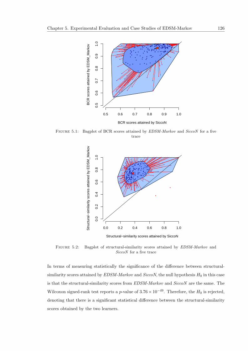
Chapter 5. Experimental Evaluation and Case Studies of EDSM-Markov 126
0.5 0.6 0.7 0.8 0.9 1.0
0.5
0.6
0.7
0.8
0.9
1.0
BCR scores attained by SiccoN
BC
R s
core
s at
tain
ed b
y E
DS
M_M
arko
v
●
●
●
●
●
●
●●
●
●
●
●
●
●
●
●
●
●
●
●
●
●
●
●
●
●
●
●
●
●
●
●
●
●
●
●
●●
●
●
●
●●
●●
●
●
●
●
●
●
●
●
●
●●
●
●
●
●
●
●●
●●
●●●
●● ●
●
●
● ●
●
●
●
●
●
● ●●
●
●●●
●
●
●●●●●●
●
●
●●
●
●●●●●●●●●●●●
●
●●
●
●●●●
●
●
●●
●
●
●
●●●
●
●●●
●
●●●
●
●●●●●●●●●
●
●
●●
●
●
●
●
●
●
●
●
●
●
●
●
●
● ●
●
●
●
●
●
●
●
●
●
●
●
●
●
●
●●
●
●
●
●
●
●
●
●
●
●
●
●
●
●
●
●●
●
●
●
●●
●
●
●
●
●●●
●
●
●●
●
●
●
●●
●
●
●●
●
●
●
●
●
●●
●
●
●
●●●●
●
●
●
●
●●
●
●
●
●
●●
●
●
●
●
●
●
●
●
●
●
●
●●
●
●●
●
●●
●
●
●
●
●
●
●
●
●
●
●
●
●
●●
●●
●
●
●
●
●
●
●
●
●
●
●
●
●
Figure 5.1: Bagplot of BCR scores attained by EDSM-Markov and SiccoN for a fivetrace
0.0 0.2 0.4 0.6 0.8 1.0
0.0
0.2
0.4
0.6
0.8
1.0
Structural−similarity scores attained by SiccoN
Str
uctu
ral−
sim
ilarit
y sc
ores
atta
ined
by
ED
SM
_Mar
kov
●●
●●
●●
●
●
●
●
●
●
●
●
●
●●
●
●●
●
●
●
●
●
●
●
●
●
●
●
●●
●
●
●
●
●
●
●
●●
●
●
●
●
●
●●
●
●
●
●
●
●
●●
●
●
●
●●
●●
●
●
●
●
●
●
●●
●
●
●
●
●
●
●●
●
●
●●
●
●
●
●
●
●
●
●
●
●●
●
●●●
●
●
●
●
●
●
●
●
●
●
●●
●
●
●●
●●
●
●
●
●
●
●
●
●●
●
●●
●
●
●
● ●●●
●
●
●
● ● ●
●
●
●●●
●
●
●
●
●
●
●
●
●
●
●
●
●
●
●
●
●
●
●
●
●
●
●
●
●
●
●
●
●
●
●●
●
●
●
●
●
●
●●
●
●
●
●●
●●
●
●
●
●
●
●
●
●
●
●
●
●
●
●
●●
●
●
●
●
●
●
●
●
●
●
●●
●
●
●
●●
●●
●
●
●
●
●
●
●
●
●
●
●
●
●
●
●
●
●
●
●
●
●
●
●
●
●
●
●
●
●
●
●
●
●
●
●
●
●
●
●
●
●●
●
●
●●
●
●
●
●
●
●
●●
●
●
●
●
●
●
●
●
●
●
●
●●
●●
●
●
Figure 5.2: Bagplot of structural-similarity scores attained by EDSM-Markov andSiccoN for a five trace
In terms of measuring statistically the significance of the difference between structural-
similarity scores attained by EDSM-Markov and SiccoN, the null hypothesis H0 in this case
is that the structural-similarity scores from EDSM-Markov and SiccoN are the same. The
Wilcoxon signed-rank test reports a p-value of 3.76× 10−49. Therefore, the H0 is rejected,
denoting that there is a significant statistical difference between the structural-similarity
scores obtained by the two learners.

Chapter 5. Experimental Evaluation and Case Studies of EDSM-Markov 127
BCR scores structural-similarity scores
EDSM-Markov v.s. SiccoN 1.97× 10−43 3.76× 10−49
Table 5.1: p-values obtained using the Wilcoxon signed-rank test for the main results
5.2.3 The Impact of the Number of Traces on the Performance of EDSM-
Markov
This section answers the first research question that is considered in Section 5.2. The
number of traces (T ) is an important parameter that should be considered in the evaluation
of the EDSM-Markov learner. The objective of this investigation is to quantify the effect of
T on the performance of EDSM-Markov compared to SiccoN. Therefore, the EDSM-Markov
learner was evaluated across different numbers of traces.
0.4
0.5
0.6
0.7
0.8
0.9
1.0
1 3 5 7Trace number
BC
R S
core
s
EDSM−Markov SiccoN
Figure 5.3: A boxplot of BCR scores attained by EDSM-Markov and SiccoN for adifferent number of traces (T )
A boxplot of the BCR scores attained by EDSM-Markov and SiccoN learners across vari-
ous settings of T is shown in Figure 5.3. It is clear that the EDSM-Markov learner inferred
LTSs with higher BCR scores compared to SiccoN when T > 1. The median value of
BCR scores obtained by EDSM-Markov is 0.99 when T = 7; In this case, the improve-
ments are reasonable. The reason behind these improvements is that Markov models were
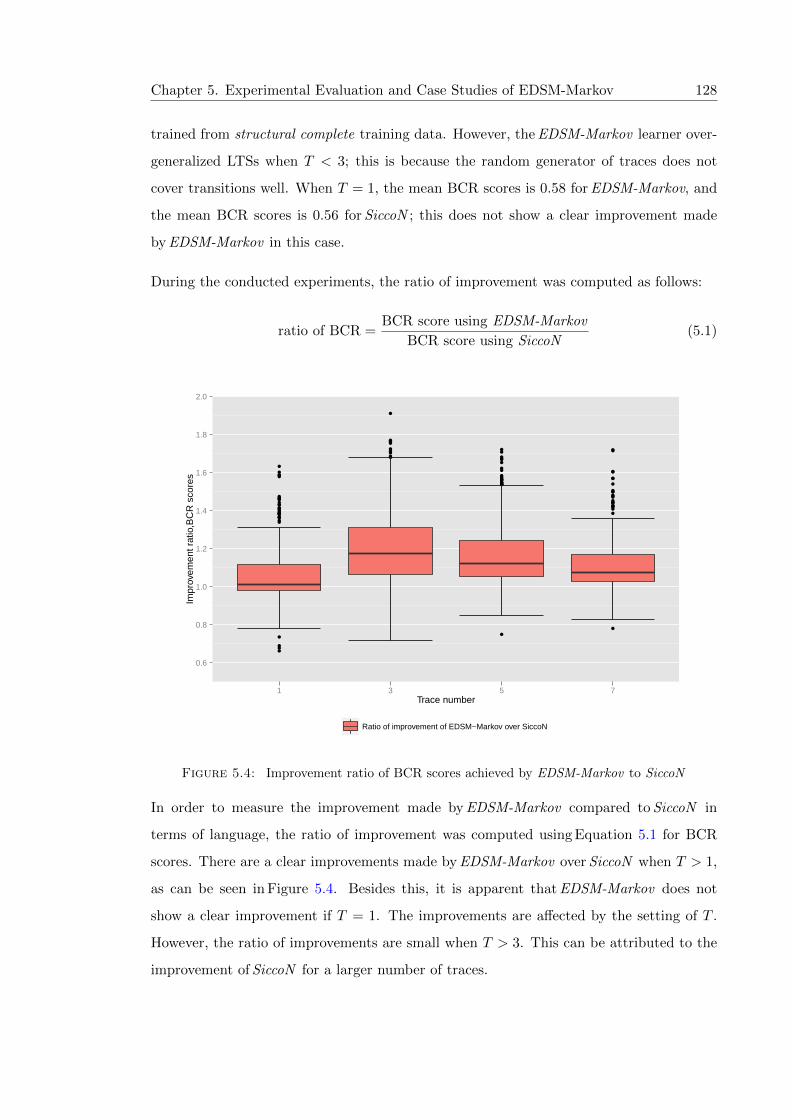
Chapter 5. Experimental Evaluation and Case Studies of EDSM-Markov 128
trained from structural complete training data. However, the EDSM-Markov learner over-
generalized LTSs when T < 3; this is because the random generator of traces does not
cover transitions well. When T = 1, the mean BCR scores is 0.58 for EDSM-Markov, and
the mean BCR scores is 0.56 for SiccoN ; this does not show a clear improvement made
by EDSM-Markov in this case.
During the conducted experiments, the ratio of improvement was computed as follows:
ratio of BCR =BCR score using EDSM-Markov
BCR score using SiccoN(5.1)
0.6
0.8
1.0
1.2
1.4
1.6
1.8
2.0
1 3 5 7Trace number
Impr
ovem
ent r
atio
,BC
R s
core
s
Ratio of improvement of EDSM−Markov over SiccoN
Figure 5.4: Improvement ratio of BCR scores achieved by EDSM-Markov to SiccoN
In order to measure the improvement made by EDSM-Markov compared to SiccoN in
terms of language, the ratio of improvement was computed using Equation 5.1 for BCR
scores. There are a clear improvements made by EDSM-Markov over SiccoN when T > 1,
as can be seen in Figure 5.4. Besides this, it is apparent that EDSM-Markov does not
show a clear improvement if T = 1. The improvements are affected by the setting of T .
However, the ratio of improvements are small when T > 3. This can be attributed to the
improvement of SiccoN for a larger number of traces.

Chapter 5. Experimental Evaluation and Case Studies of EDSM-Markov 129
Additionally, the small ratio of improvement does not mean that the EDSM-Markov learner
performed badly, but it is because SiccoN inferred LTSs with BCR scores close to those
obtained using EDSM-Markov. The SiccoN learner tends to block invalid mergers correctly
in case where T is large. This is intuitive because SiccoN benefits from the performance
of EDSM that performs better on heavily branching traces.
0.0
0.2
0.4
0.6
0.8
1.0
1 3 5 7Trace number
stru
ctur
al−
sim
ilarit
y sc
ores
EDSM−Markov SiccoN
Figure 5.5: A boxplot of structural-similarity scores attained by EDSM-Markov andSiccoN for a different number of traces
The effect of T on the structural-similarity scores obtained using EDSM-Markov and Sic-
coN is shown in Figure 5.5. Judging by the boxplots shown above, it is clear that the
structural-similarity scores achieved by EDSM-Markov increase while T increases. This
implies that the Markov models were trained enough to identify inconsistencies during
merging states. It can be seen from Figure 5.5 that EDSM-Markov, at every setting of T ,
inferred LTSs with higher structural-similarity scores compared to SiccoN. It is obvious
that EDSM-Markov achieves reasonable structural-similarity scores when T > 5.
Ratio of structural difference =Structural-similarity score using EDSM-Markov
Structural-similarity score using SiccoN(5.2)

Chapter 5. Experimental Evaluation and Case Studies of EDSM-Markov 130
0.6
0.9
1.2
1.5
1.8
2.1
2.4
2.7
3.0
3.3
3.6
3.9
4.2
4.5
1 3 5 7Trace number
Impr
ovem
ent r
atio
,str
uctu
ral−
sim
ilair
ty s
core
s
Ratio of improvement of EDSM−Markov over SiccoN
Figure 5.6: Improvement ratio of structural-similarity scores achieved by EDSM-Markov to SiccoN
The ratio of improvement of the structural-similarity scores achieved by EDSM-Markov
over SiccoN learners was computed using Equation 5.2; this ratio is shown in Figure 5.6. It
appears from Figure 5.6 that, the structural-similarity scores of LTSs inferred using EDSM-
Markov are higher than those obtained using SiccoN. This is because SiccoN tends to
prevent merging equivalent states that should be merged since training data is sparse.
Table 5.2 shows the p-values obtained using the paired Wilcoxon signed-rank test after
comparing the BCR and structural-similarity scores attained by EDSM-Markov and SiccoN.
The null hypothesis H0 is that SiccoN produces similar results to EDSM-Markov. In all
cases, the considered H0 can be rejected because the p-values are less than 0.05. This de-
notes that there is a clear statistical difference between the scores obtained using EDSM-
Markov compared to SiccoN. In addition, Table 5.2 provides the mean values for BCR and
structural-similarity scores. The mean BCR score for EDSM-Markov is higher than the
mean BCR score for SiccoN, as shown in Table 5.2.

Chapter 5. Experimental Evaluation and Case Studies of EDSM-Markov 131
T
p-value of
E-M vs SiccoNMean BCR
Mean
structural similarity
BCRstructural
similarityE-M SiccoN E-M SiccoN
1 4.49× 10−07 4.40× 10−46 0.58 0.56 0.50 0.31
3 7.33× 10−40 2.38× 10−49 0.85 0.71 0.68 0.35
5 1.97× 10−43 3.76× 10−49 0.93 0.80 0.76 0.41
7 2.09× 10−39 2.07× 10−49 0.96 0.86 0.80 0.45
Table 5.2: p-values obtained using the Wilcoxon signed-rank test of comparing EDSM-Markov v.s. SiccoN across different number of traces
5.2.4 The Impact of Alphabet Size on the Performance of EDSM-Markov
This section answers the second research question that is considered early in Section 5.2.
In order to evaluate different types of LTS, an alphabet size is a significant factor to
consider for evaluating the performance of the EDSM-Markov learner. In Section 5.2.3,
the alphabet size in the experiment was two times the number of states |Σ| = 2 ∗ Q.
Hence, experiments were conducted to measure the impact of various sizes of alphabet on
the quality of the inferred LTSs. The size of the alphabet was modified in stages, and it
ranged with values between 14 and 4 times the alphabet size used in Section 5.2.2. In this
way, an alphabet multiplier parameter m was introduced to vary the alphabet size such
that |Σ| = m ∗ |Q|, and |Σ| ranged between 12 ∗ |Q| and 8 ∗ |Q| in this experiment. Positive
sequences of length 2 ∗ |Q|2 were used as training data. The number of traces (T ) ranged
from 1 to 7, incrementing by 2. Thus, the variance in this experiment is based on both
|Σ| and T .
The boxplots of the BCR scores obtained by EDSM-Markov and SiccoN for all differ-
ent alphabet sizes considered are illustrated in Figure 5.7. The BCR scores attained by
the EDSM-Markov learner appear to be optimal when m > 1 and T ≥ 5. However, the
EDSM-Markov learner over-generalized LTSs when m = 0.5 and T < 7. The reason be-
hind the over-generalization is that whenever a pair of states are merged, new labels of
outgoing transitions would be added to the merged node which are incorrectly predicted
as permitted to follow it; in this case, inconsistencies are not detected.
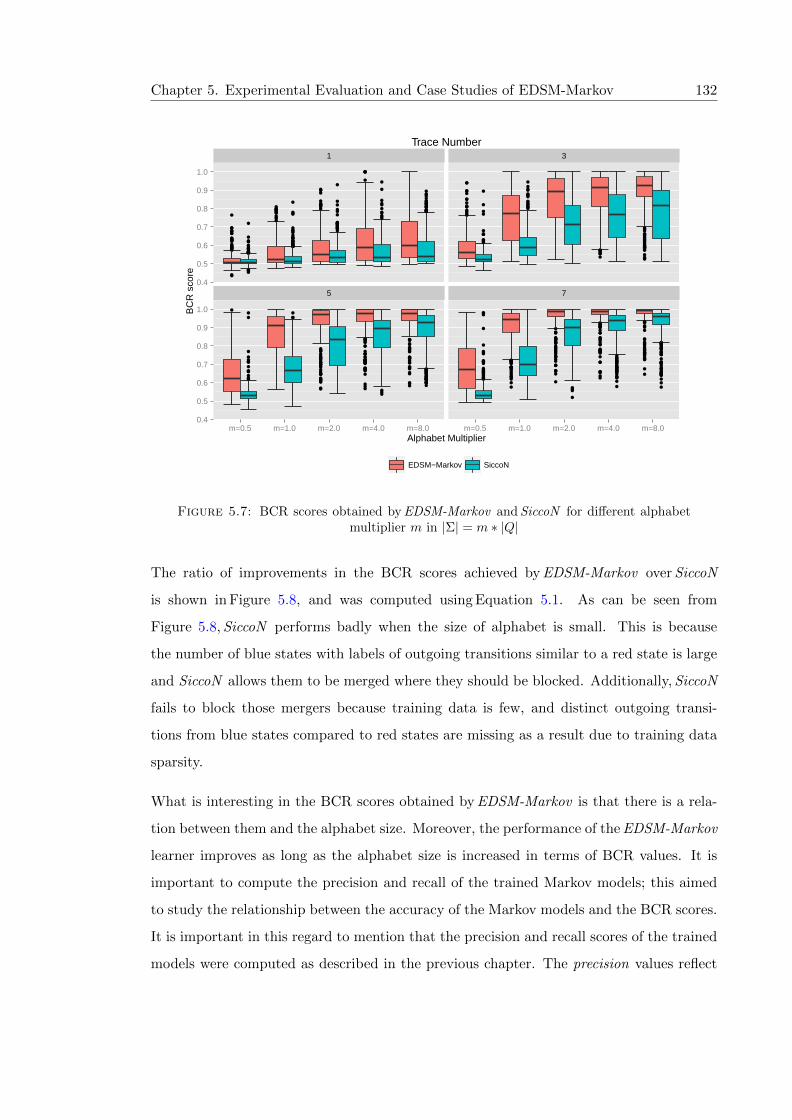
Chapter 5. Experimental Evaluation and Case Studies of EDSM-Markov 132
1 3
5 70.4
0.5
0.6
0.7
0.8
0.9
1.0
0.4
0.5
0.6
0.7
0.8
0.9
1.0
m=0.5 m=1.0 m=2.0 m=4.0 m=8.0 m=0.5 m=1.0 m=2.0 m=4.0 m=8.0Alphabet Multiplier
BC
R s
core
EDSM−Markov SiccoN
Trace Number
Figure 5.7: BCR scores obtained by EDSM-Markov and SiccoN for different alphabetmultiplier m in |Σ| = m ∗ |Q|
The ratio of improvements in the BCR scores achieved by EDSM-Markov over SiccoN
is shown in Figure 5.8, and was computed using Equation 5.1. As can be seen from
Figure 5.8, SiccoN performs badly when the size of alphabet is small. This is because
the number of blue states with labels of outgoing transitions similar to a red state is large
and SiccoN allows them to be merged where they should be blocked. Additionally, SiccoN
fails to block those mergers because training data is few, and distinct outgoing transi-
tions from blue states compared to red states are missing as a result due to training data
sparsity.
What is interesting in the BCR scores obtained by EDSM-Markov is that there is a rela-
tion between them and the alphabet size. Moreover, the performance of the EDSM-Markov
learner improves as long as the alphabet size is increased in terms of BCR values. It is
important to compute the precision and recall of the trained Markov models; this aimed
to study the relationship between the accuracy of the Markov models and the BCR scores.
It is important in this regard to mention that the precision and recall scores of the trained
models were computed as described in the previous chapter. The precision values reflect
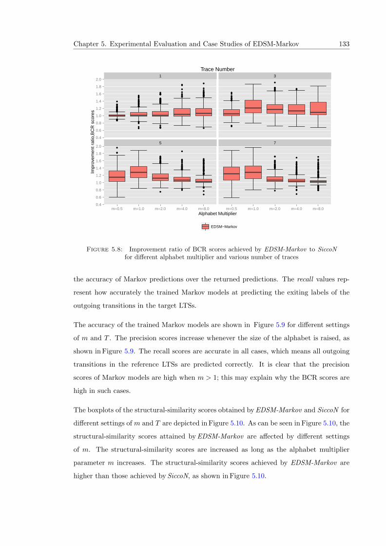
Chapter 5. Experimental Evaluation and Case Studies of EDSM-Markov 133
1 3
5 70.4
0.6
0.8
1.0
1.2
1.4
1.6
1.8
2.0
0.4
0.6
0.8
1.0
1.2
1.4
1.6
1.8
2.0
m=0.5 m=1.0 m=2.0 m=4.0 m=8.0 m=0.5 m=1.0 m=2.0 m=4.0 m=8.0Alphabet Multiplier
Impr
ovem
ent r
atio
,BC
R s
core
s
EDSM−Markov
Trace Number
Figure 5.8: Improvement ratio of BCR scores achieved by EDSM-Markov to SiccoNfor different alphabet multiplier and various number of traces
the accuracy of Markov predictions over the returned predictions. The recall values rep-
resent how accurately the trained Markov models at predicting the exiting labels of the
outgoing transitions in the target LTSs.
The accuracy of the trained Markov models are shown in Figure 5.9 for different settings
of m and T . The precision scores increase whenever the size of the alphabet is raised, as
shown in Figure 5.9. The recall scores are accurate in all cases, which means all outgoing
transitions in the reference LTSs are predicted correctly. It is clear that the precision
scores of Markov models are high when m > 1; this may explain why the BCR scores are
high in such cases.
The boxplots of the structural-similarity scores obtained by EDSM-Markov and SiccoN for
different settings of m and T are depicted in Figure 5.10. As can be seen in Figure 5.10, the
structural-similarity scores attained by EDSM-Markov are affected by different settings
of m. The structural-similarity scores are increased as long as the alphabet multiplier
parameter m increases. The structural-similarity scores achieved by EDSM-Markov are
higher than those achieved by SiccoN, as shown in Figure 5.10.

Chapter 5. Experimental Evaluation and Case Studies of EDSM-Markov 134
1 3
5 70
20
40
60
80
100
0
20
40
60
80
100
m=0.5 m=1.0 m=2.0 m=4.0 m=8.0 m=0.5 m=1.0 m=2.0 m=4.0 m=8.0Alphabet Multiplier
Per
cent
age
%
Precision Recall
Trace Number
Figure 5.9: Accuracy of Markov predictions for a different alphabet multiplier acrossvarious number of traces
1 3
5 70.0
0.2
0.4
0.6
0.8
1.0
0.0
0.2
0.4
0.6
0.8
1.0
m=0.5 m=1.0 m=2.0 m=4.0 m=8.0 m=0.5 m=1.0 m=2.0 m=4.0 m=8.0Alphabet Multiplier
stru
ctur
al s
imila
rity
scor
e
EDSM−Markov SiccoN
Trace Number
Figure 5.10: Structural-similarity scores of EDSM-Markov and SiccoN for differentalphabet multiplier m in |Σ| = m ∗ |Q|
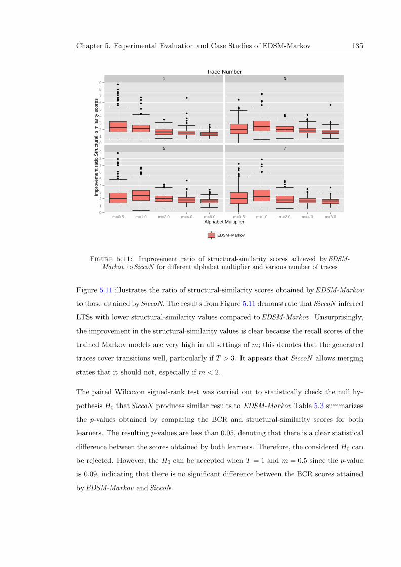
Chapter 5. Experimental Evaluation and Case Studies of EDSM-Markov 135
1 3
5 70
1
2
3
4
5
6
7
8
9
0
1
2
3
4
5
6
7
8
9
m=0.5 m=1.0 m=2.0 m=4.0 m=8.0 m=0.5 m=1.0 m=2.0 m=4.0 m=8.0Alphabet Multiplier
Impr
ovem
ent r
atio
,Str
uctu
ral−
sim
ilarit
y sc
ores
EDSM−Markov
Trace Number
Figure 5.11: Improvement ratio of structural-similarity scores achieved by EDSM-Markov to SiccoN for different alphabet multiplier and various number of traces
Figure 5.11 illustrates the ratio of structural-similarity scores obtained by EDSM-Markov
to those attained by SiccoN. The results from Figure 5.11 demonstrate that SiccoN inferred
LTSs with lower structural-similarity values compared to EDSM-Markov. Unsurprisingly,
the improvement in the structural-similarity values is clear because the recall scores of the
trained Markov models are very high in all settings of m; this denotes that the generated
traces cover transitions well, particularly if T > 3. It appears that SiccoN allows merging
states that it should not, especially if m < 2.
The paired Wilcoxon signed-rank test was carried out to statistically check the null hy-
pothesis H0 that SiccoN produces similar results to EDSM-Markov. Table 5.3 summarizes
the p-values obtained by comparing the BCR and structural-similarity scores for both
learners. The resulting p-values are less than 0.05, denoting that there is a clear statistical
difference between the scores obtained by both learners. Therefore, the considered H0 can
be rejected. However, the H0 can be accepted when T = 1 and m = 0.5 since the p-value
is 0.09, indicating that there is no significant difference between the BCR scores attained
by EDSM-Markov and SiccoN.

Chapter 5. Experimental Evaluation and Case Studies of EDSM-Markov 136
m T
p-value of
E-M vs SiccoNMean BCR
Mean
structural-similarity
BCRstructural
similarityE-M SiccoN E-M SiccoN
0.5
1 0.09 2.74× 10−47 0.52 0.52 0.28 0.13
3 3.32× 10⁻²⁴ 3.87× 10⁻³⁵ 0.59 0.54 0.29 0.16
5 6.98× 10−37 9.34× 10−37 0.65 0.54 0.31 0.16
7 3.27× 10−38 2.44× 10⁻³¹ 0.69 0.55 0.33 0.17
1.0
1 2.82× 10−09 3.89× 10−47 0.56 0.53 0.42 0.21
3 5.24× 10−41 9.05× 10−49 0.76 0.61 0.55 0.24
5 3.92× 10−48 4.71× 10−48 0.87 0.68 0.62 0.28
7 9.88× 10−46 8.19× 10−48 0.91 0.72 0.66 0.31
2.0
1 4.49× 10−07 4.40× 10−46 0.58 0.56 0.50 0.31
3 7.33× 10−40 2.38× 10−49 0.85 0.71 0.68 0.35
5 1.97× 10−43 3.76× 10−49 0.93 0.8 0.76 0.41
7 2.09× 10−39 2.07× 10−49 0.96 0.86 0.80 0.45
4.0
1 2.23× 10⁻¹⁵ 2.06× 10−45 0.62 0.57 0.55 0.37
3 6.96× 10⁻³⁵ 3.09× 10−50 0.88 0.76 0.72 0.42
5 8.79× 10−38 1.66× 10−50 0.94 0.85 0.80 0.45
7 3.00× 10−36 3.98× 10−49 0.97 0.9 0.84 0.51
8.0
1 5.59× 10⁻¹⁶ 9.36× 10−37 0.64 0.58 0.55 0.42
3 2.13× 10⁻³⁵ 1.75× 10−49 0.89 0.77 0.73 0.46
5 4.48× 10⁻³¹ 1.97× 10−50 0.95 0.89 0.80 0.50
7 1.24× 10⁻²⁷ 4.81× 10−50 0.97 0.92 0.85 0.53
Table 5.3: Wilcoxon signed rank test with continuity correction of comparing EDSM-Markov v.s. SiccoN using various alphabet multiplier
5.2.5 The Impact of the Length of Traces on the Performance of EDSM-
Markov
The third research question considered in Section 5.2 is to investigate the influence of the
length of a few traces on the performance of the EDSM-Markov learner; the findings in this
section answer this question. One of the most important factors to evaluate the efficiency
of inference algorithms is the capability to generate good LTSs from different lengths of
traces. In the previous sections, the length of traces was given by length = 2 ∗ |Q|2.
Therefore, experiments were carried out to measure the effect of different lengths of traces
on the performance of the proposed learner. The length of traces was given by l ∗ 2 ∗ |Q|2

Chapter 5. Experimental Evaluation and Case Studies of EDSM-Markov 137
where the parameter l denotes the length multiplier, and introduced to vary the length
of traces. Besides, the EDSM-Markov learner on different lengths of traces and various
alphabet sizes as well. Thus, the alphabet size was given by |Σ| = m ∗ |Q|, and |Σ| ranged
between 12 ∗ |Q| and 2 ∗ |Q| in the conducted experiment.
5.2.5.1 When m = 2.0
Figure 5.12 shows the boxplots of the BCR scores obtained using EDSM-Markov and SiccoN
when m = 2. As expected, the performance of EDSM-Markov is affected by the length
of traces where long ones result in generating good LTSs; this is because transitions are
covered well. The median value of the BCR scores obtained by EDSM-Markov is 0.99
when l = 2 and T = 7. It appears from Figure 5.12 that the exact LTSs can be inferred if
the provided traces are very long. The EDSM-Markov learner inferred LTSs with higher
BCR values compared to Sicco in the majority of cases as shown in Figure 5.12.
1 3
5 70.4
0.5
0.6
0.7
0.8
0.9
1.0
0.4
0.5
0.6
0.7
0.8
0.9
1.0
L=0.125 L=0.25 L=0.5 L=1.0 L=2.0 L=0.125 L=0.25 L=0.5 L=1.0 L=2.0Trace Length Muliplier
BC
R s
core
EDSM−Markov SiccoN
Trace Number
Figure 5.12: Blots of BCR scores obtained by EDSM-Markov and SiccoN for differentsetting of l and various numbers of traces where m = 2.0, the length of traces is given by
= l ∗ 2 ∗ |Q|2
It can be seen from Figure 5.12 that the BCR scores obtained by EDSM-Markov are very
low when T = 1 and l < 2.0. This is because the generated traces cover transitions well,

Chapter 5. Experimental Evaluation and Case Studies of EDSM-Markov 138
as shown in Figure 5.13. Moreover, the Markov models were not trained well to make
predictions correctly. Thus, new prefix paths of length k were added to the merged node
during the state-merging process where Markov models did not see them; this caused
inconsistency scores to be too large. Hence, many pairs of states that should be merged
were blocked.
1 3
5 710
20
30
40
50
60
70
80
90
100
10
20
30
40
50
60
70
80
90
100
L=0.125 L=0.25 L=0.5 L=1.0 L=2.0 L=0.125 L=0.25 L=0.5 L=1.0 L=2.0Trace Length Muliplier
tran
sitio
n co
vera
ge
The percentage of transition coverage
Trace Number
Figure 5.13: Transition coverage for different setting of l and various numbers of traceswhere m = 2.0 and the length of traces is given by = l ∗ 2 ∗ |Q|2
Figure 5.14 presents boxplots of the structural-similarity scores achieved by EDSM-Markov
and SiccoN. As can be seen from Figure 5.14, the structural-similarity scores of the inferred
LTSs using EDSM-Markov climbs steadily with the increase in l. The structural-similarity
scores of LTSs inferred using EDSM-Markov are higher than those obtained using SiccoN.
Table 5.4 gives the p-values obtained by the paired Wilcoxon signed-rank test after com-
paring the BCR and structural-similarity scores of both algorithms. The null hypothesis
H0 to be tested in this study is that there is no difference between the scores attained
by EDSM-Markov and SiccoN. The p-values show that there is clear evidence that EDSM-
Markov inferred LTSs with structural-similarity scores higher than SiccoN. The resulting
p-values are less than 0.05, supporting the clear improvement shown in Figure 5.14. Thus,
the null hypothesis H0 is rejected. However, when comparing the BCR scores attained by

Chapter 5. Experimental Evaluation and Case Studies of EDSM-Markov 139
1 3
5 70.0
0.2
0.4
0.6
0.8
1.0
0.0
0.2
0.4
0.6
0.8
1.0
L=0.125 L=0.25 L=0.5 L=1.0 L=2.0 L=0.125 L=0.25 L=0.5 L=1.0 L=2.0Trace Length Muliplier
stru
ctur
al s
imila
rity
scor
e
EDSM−Markov SiccoN
Trace Number
Figure 5.14: Structural-similarity scores obtained by EDSM-Markov and SiccoN fordifferent l, l ∗ |Q| ∗ |Σ| = 2 ∗ l ∗ |Q|2
both learners, the H0 can be accepted when l = 0.125, denoting that there is no statis-
tical difference between the scores. With T = 1 and l = 0.25, the p-value is 0.79 when
comparing the BCR scores attained by both learners, and the H0 can be accepted.

Chapter 5. Experimental Evaluation and Case Studies of EDSM-Markov 140
l T
p-value of
E-M Vs.SiccoNMean BCR
Mean
structural similarity
BCRStructural
similarityE-M SiccoN E-M SiccoN
0.125
1 0.98 2.95× 10−08 0.5 0.5 0.36 0.32
3 0.38 1.43× 10⁻²⁵ 0.54 0.54 0.43 0.35
5 0.33 5.29× 10⁻³⁰ 0.58 0.58 0.49 0.39
7 0.37 6.48× 10⁻³¹ 0.65 0.64 0.54 0.43
0.25
1 0.79 6.42× 10⁻²⁷ 0.51 0.51 0.39 0.31
3 3.02× 10−07 2.73× 10−37 0.59 0.57 0.49 0.35
5 5.79× 10⁻¹¹ 3.66× 10−44 0.70 0.66 0.58 0.40
7 3.68× 10⁻¹⁶ 2.05× 10−45 0.79 0.74 0.64 0.43
0.5
1 0.001 3.35× 10−38 0.53 0.52 0.44 0.31
3 2.71× 10⁻²⁸ 4.03× 10−46 0.72 0.63 0.58 0.36
5 2.38× 10⁻³² 8.41× 10−49 0.84 0.74 0.69 0.40
7 1.27× 10−36 5.69× 10−50 0.90 0.81 0.73 0.44
1.0
1 4.49× 10−07 4.40× 10−46 0.59 0.56 0.50 0.31
3 7.33× 10−40 2.38× 10−49 0.85 0.71 0.68 0.35
5 1.97× 10−43 3.76× 10−49 0.93 0.81 0.76 0.41
7 2.09× 10−39 2.07× 10−49 0.96 0.86 0.80 0.45
2.0
1 2.69× 10⁻¹⁷ 1.26× 10−47 0.68 0.60 0.57 0.30
3 4.51× 10−43 2.05× 10−50 0.91 0.74 0.74 0.34
5 2.36× 10−41 3.59× 10−50 0.95 0.83 0.82 0.39
7 5.74× 10−46 4.73× 10−50 0.98 0.88 0.84 0.44
Table 5.4: p-values obtained using the Wilcoxon signed-rank test by comparing EDSM-Markov v.s. SiccoN across different number of traces where m=2.0
5.2.5.2 When m = 0.5
In the previous section, the m parameter was 2. In this section, the performance of EDSM-
Markov is evaluated for different lengths when m = 0.5. Figure 5.15 shows the BCR scores
obtained by EDSM-Markov and SiccoN when m = 0.5. Indeed, unlike when m = 2.0,
the BCR scores achieved by EDSM-Markov are very low even for long traces, especially
when T < 5. The precision scores of the trained Markov models are too low and this may
contribute to the low BCR scores. Despite this, the BCR scores of the generated LTSs
using EDSM-Markov are higher than SiccoN when T > 3. When T = 7, for instance, the
average BCR scores attained by EDSM-Markov is 0.70 at l = 2.0 and 0.65 at l = 0.5. This

Chapter 5. Experimental Evaluation and Case Studies of EDSM-Markov 141
indicates that the length of the traces affects the performance of EDSM-Markov.
1 3
5 70.4
0.5
0.6
0.7
0.8
0.9
1.0
0.4
0.5
0.6
0.7
0.8
0.9
1.0
L=0.125 L=0.25 L=0.5 L=1.0 L=2.0 L=0.125 L=0.25 L=0.5 L=1.0 L=2.0Trace Length Muliplier
BC
R s
core
EDSM−Markov SiccoN
Trace Number
Figure 5.15: BCR scores obtained by EDSM-Markov and SiccoN for different l wherem = 0.5, = l ∗ 2 ∗ |Q|2
1 3
5 70.0
0.2
0.4
0.6
0.8
1.0
0.0
0.2
0.4
0.6
0.8
1.0
L=0.125 L=0.25 L=0.5 L=1.0 L=2.0 L=0.125 L=0.25 L=0.5 L=1.0 L=2.0Trace Length Muliplier
stru
ctur
al s
imila
rity
scor
e
EDSM−Markov SiccoN
Trace Number
Figure 5.16: Structural-similarity scores obtained by EDSM-Markov and SiccoN fordifferent l where m = 0.5, = l ∗ 2 ∗ |Q|2

Chapter 5. Experimental Evaluation and Case Studies of EDSM-Markov 142
It is necessary to provide insight about the impact of the length of traces on the structure
of the inferred LTSs. Figure 5.16 illustrates the structural-similarity scores of LTSs in-
ferred using EDSM-Markov and SiccoN. The scores achieved by EDSM-Markov are higher
than those attained by SiccoN. The improvement made by EDSM-Markov over SiccoN in
terms of the structural-similarity is clear even when T = 1 and l = 0.125. The aver-
age structural-similarity scores obtained by EDSM-Markov increased by 70.59% compared
to SiccoN when T = 1and l = 0.125.
Table 5.5 summarizes the p-values computed using the paired Wilcoxon signed-rank test
for the BCR and structural-similarity scores. The null hypothesis H0 in this investigation
is that the scores attained by EDSM-Markov and SiccoN are the same. The p-values show
that the scores obtained by learner are significant at the 0.05 level in the majority of cases.
In such cases, the null hypothesis H0 is rejected. When T = 1 and l = 0.25, l = 0.5, and
l = 1.0, the H0 can be accepted because the p-values are higher than 0.05, which means
that the results are not significant in these cases.
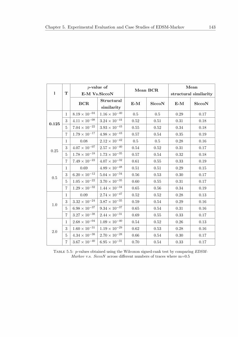
Chapter 5. Experimental Evaluation and Case Studies of EDSM-Markov 143
l T
p-value of
E-M Vs.SiccoNMean BCR
Mean
structural similarity
BCRStructural
similarityE-M SiccoN E-M SiccoN
0.125
1 8.19× 10−04 1.16× 10−40 0.5 0.5 0.29 0.17
3 4.11× 10−08 3.24× 10−44 0.52 0.51 0.31 0.18
5 7.04× 10⁻²² 3.93× 10−43 0.55 0.52 0.34 0.18
7 1.79× 10⁻¹⁷ 4.98× 10−43 0.57 0.54 0.35 0.19
0.25
1 0.08 2.12× 10−42 0.5 0.5 0.28 0.16
3 4.07× 10−07 2.57× 10−40 0.54 0.52 0.31 0.17
5 1.78× 10⁻¹⁸ 1.73× 10⁻³⁵ 0.57 0.54 0.32 0.18
7 7.49× 10⁻²² 4.07× 10⁻³² 0.61 0.55 0.33 0.19
0.5
1 0.69 4.89× 10−48 0.51 0.51 0.29 0.15
3 6.20× 10⁻¹² 5.04× 10⁻³⁴ 0.56 0.53 0.30 0.17
5 1.05× 10⁻²² 3.70× 10⁻³⁵ 0.60 0.55 0.31 0.17
7 1.29× 10⁻³² 1.44× 10⁻³⁴ 0.65 0.56 0.34 0.19
1.0
1 0.09 2.74× 10−47 0.52 0.52 0.28 0.13
3 3.32× 10⁻²⁴ 3.87× 10⁻³⁵ 0.59 0.54 0.29 0.16
5 6.98× 10−37 9.34× 10−37 0.65 0.54 0.31 0.16
7 3.27× 10−38 2.44× 10⁻³¹ 0.69 0.55 0.33 0.17
2.0
1 2.68× 10−04 1.09× 10−40 0.54 0.52 0.26 0.13
3 1.60× 10⁻³¹ 1.19× 10⁻²⁹ 0.62 0.53 0.28 0.16
5 4.34× 10−38 2.70× 10⁻²⁸ 0.66 0.54 0.30 0.17
7 3.67× 10−40 6.95× 10⁻³¹ 0.70 0.54 0.33 0.17
Table 5.5: p-values obtained using the Wilcoxon signed-rank test by comparing EDSM-Markov v.s. SiccoN across different numbers of traces where m=0.5

Chapter 5. Experimental Evaluation and Case Studies of EDSM-Markov 144
5.2.5.3 When m = 1.0
In this section, the outcomes of evaluating the performance of the EDSM-Markov learner
with different lengths of traces are presented. The size of the alphabet is given by Σ =
m × |Q| where m = 1.0. Figure 5.17 shows the BCR scores obtained by EDSM-Markov
and SiccoN when m = 1.0. The graph illustrates that there is a gradual increase in
the BCR scores obtained using EDSM-Markov with the increase of the lengths of traces.
In addition, the BCR scores obtained by EDSM-Markov are higher than those obtained
by SiccoN when T > 1.
It is worth noting that the BCR scores attained by EDSM-Markov are higher than those
obtained by the same learner when l = 0.5. This is because the precision scores of the
Markov models when m = 1.0 are higher than those of Markov models when m = 0.5.
1 3
5 70.4
0.5
0.6
0.7
0.8
0.9
1.0
0.4
0.5
0.6
0.7
0.8
0.9
1.0
L=0.125 L=0.25 L=0.5 L=1.0 L=2.0 L=0.125 L=0.25 L=0.5 L=1.0 L=2.0Trace Length Muliplier
BC
R s
core
EDSM−Markov SiccoN
Trace Number
Figure 5.17: BCR scores obtained by EDSM-Markov and SiccoN for different settingof l and various numbers of traces where m = 1.0 and the length of traces is given by
= l ∗ 2 ∗ |Q|2
Figure 5.18 shows boxplots of the structural-similarity scores obtained by EDSM-Markov
and SiccoN. In Figure 5.14, there is a clear tendency for the structural-similarity scores

Chapter 5. Experimental Evaluation and Case Studies of EDSM-Markov 145
of the inferred LTSs using EDSM-Markov to increase while l increases. The structural-
similarity scores of the inferred LTSs using SiccoN are very low compared to EDSM-
Markov.
1 3
5 70.0
0.1
0.2
0.3
0.4
0.5
0.6
0.7
0.8
0.9
1.0
0.0
0.1
0.2
0.3
0.4
0.5
0.6
0.7
0.8
0.9
1.0
L=0.125 L=0.25 L=0.5 L=1.0 L=2.0 L=0.125 L=0.25 L=0.5 L=1.0 L=2.0Trace Length Muliplier
stru
ctur
al s
imila
rity
scor
e
EDSM−Markov SiccoN
Trace Number
Figure 5.18: structural difference scores obtained by EDSM-Markov for trace lengthmultiplier l setting the length of each of the 5 traces to l ∗ |Q| ∗ |Σ| = 2 ∗ l ∗ |Q|2
Table 5.6 summarizes the statistical test results using the paired Wilcoxon signed-rank test
for the BCR and structural-similarity scores. The null hypothesis H0 considered in this
research question is that the scores of the inferred LTS using EDSM-Markov and SiccoN
are the same. When l = 0.125 and the number of traces is 1, EDSM-Markov does not
show a significant difference compared to SiccoN in terms of BCR scores. However, the
p-values are below the 0.05 significance level in cases where l > 0.125, so the considered
null hypothesis can be rejected.
The fourth column in Table 5.6 summarizes the statistical test results obtained using the
Wilcoxon signed-rank test for structural-similarity scores. It is clear that the resulted
p-values are below the 0.05 significance level in all cases. Therefore, the H0 is rejected
since in the majority of cases, it denotes that the structural-similarity scores obtained
by EDSM-Markov are higher than scores obtained by SiccoN.
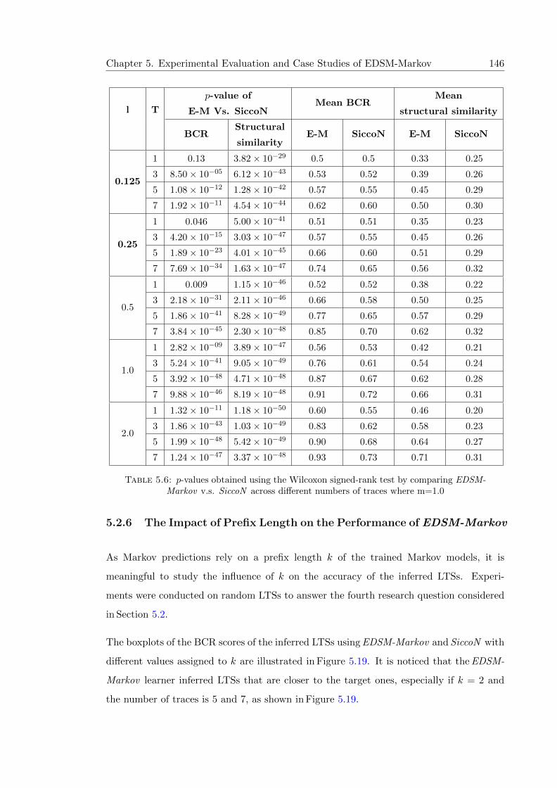
Chapter 5. Experimental Evaluation and Case Studies of EDSM-Markov 146
l T
p-value of
E-M Vs. SiccoNMean BCR
Mean
structural similarity
BCRStructural
similarityE-M SiccoN E-M SiccoN
0.125
1 0.13 3.82× 10⁻²⁹ 0.5 0.5 0.33 0.25
3 8.50× 10−05 6.12× 10−43 0.53 0.52 0.39 0.26
5 1.08× 10⁻¹² 1.28× 10−42 0.57 0.55 0.45 0.29
7 1.92× 10⁻¹¹ 4.54× 10−44 0.62 0.60 0.50 0.30
0.25
1 0.046 5.00× 10−41 0.51 0.51 0.35 0.23
3 4.20× 10⁻¹⁵ 3.03× 10−47 0.57 0.55 0.45 0.26
5 1.89× 10⁻²³ 4.01× 10−45 0.66 0.60 0.51 0.29
7 7.69× 10⁻³⁴ 1.63× 10−47 0.74 0.65 0.56 0.32
0.5
1 0.009 1.15× 10−46 0.52 0.52 0.38 0.22
3 2.18× 10⁻³¹ 2.11× 10−46 0.66 0.58 0.50 0.25
5 1.86× 10−41 8.28× 10−49 0.77 0.65 0.57 0.29
7 3.84× 10−45 2.30× 10−48 0.85 0.70 0.62 0.32
1.0
1 2.82× 10−09 3.89× 10−47 0.56 0.53 0.42 0.21
3 5.24× 10−41 9.05× 10−49 0.76 0.61 0.54 0.24
5 3.92× 10−48 4.71× 10−48 0.87 0.67 0.62 0.28
7 9.88× 10−46 8.19× 10−48 0.91 0.72 0.66 0.31
2.0
1 1.32× 10⁻¹¹ 1.18× 10−50 0.60 0.55 0.46 0.20
3 1.86× 10−43 1.03× 10−49 0.83 0.62 0.58 0.23
5 1.99× 10−48 5.42× 10−49 0.90 0.68 0.64 0.27
7 1.24× 10−47 3.37× 10−48 0.93 0.73 0.71 0.31
Table 5.6: p-values obtained using the Wilcoxon signed-rank test by comparing EDSM-Markov v.s. SiccoN across different numbers of traces where m=1.0
5.2.6 The Impact of Prefix Length on the Performance of EDSM-Markov
As Markov predictions rely on a prefix length k of the trained Markov models, it is
meaningful to study the influence of k on the accuracy of the inferred LTSs. Experi-
ments were conducted on random LTSs to answer the fourth research question considered
in Section 5.2.
The boxplots of the BCR scores of the inferred LTSs using EDSM-Markov and SiccoN with
different values assigned to k are illustrated in Figure 5.19. It is noticed that the EDSM-
Markov learner inferred LTSs that are closer to the target ones, especially if k = 2 and
the number of traces is 5 and 7, as shown in Figure 5.19.

Chapter 5. Experimental Evaluation and Case Studies of EDSM-Markov 147
1 3
5 70.4
0.5
0.6
0.7
0.8
0.9
1.0
0.4
0.5
0.6
0.7
0.8
0.9
1.0
EDSM−Markov k=1 EDSM−Markov k=2 EDSM−Markov k=3 SiccoN EDSM−Markov k=1 EDSM−Markov k=2 EDSM−Markov k=3 SiccoN
Prefix Length
BC
R s
core
s
EDSM−Markov k=1 EDSM−Markov k=2 EDSM−Markov k=3 SiccoN
Trace Number
Figure 5.19: BCR scores for EDSM-Markov and SiccoN for a different prefix length,and various number of traces
As can be seen in Figure 5.19, a prefix length of two (k = 2) appears to be optimal
compared to k = 1 and 3. It is clear that the EDSM-Markov learner performs better
than SiccoN when k = 1 and 2 and the number of traces is more than 1. This is because
EDSM-Markov detects inconsistencies accurately during the comparison of pairs of states
to prevent merging invalid ones using the IScore heuristic. Moreover, the inferred LTSs
using EDSM-Markov when k = 2 are better than those inferred if k = 1, and this is
because the precision scores of the trained Markov model if K = 2 are higher than the
precision scores if k = 1, as shown in Figure 5.20.
It is important to highlight that, whenever two states are considered for merging, new
labels of transitions might be added to the merged node; if they are incorrectly predicted
to follow the node, then inconsistencies will not be detected during the computation of
the IScore score. In the conducted experiments, this occurred when k = 1 since the Markov
precision is very low in this case, as shown in Figure 5.20. With the number of trace being
one, the BCR scores are not as good as when the number of traces are 5 and 7. This may
be because many predictions of labels of transitions are missed out due to the sparsity of
data. Since a complete table predicting transitions based on the history of k transitions

Chapter 5. Experimental Evaluation and Case Studies of EDSM-Markov 148
1 3
5 70
20
40
60
80
100
0
20
40
60
80
100
k=1 k=2 k=3 k=1 k=2 k=3Prefix Length
Per
cent
age
Precision Recall
Trace Number
Figure 5.20: Accuracy of Markov predictions for a different prefix length across differentnumber of traces
has |Σ|k entries, one would expect larger values of k to correspond to fewer predicted
transitions and thus lower recall values.
Figure 5.21 illustrates the ratio of improvement of BCR scores for LTSs inferred using
EDSM-Markov to SiccoN. It appears that the BCR scores improved when K < 3, as shown
in Figure 5.21. For a prefix length of 3, many Markov predictions are missed to prevent
merging of an inequivalent pair of states. Despite the high values of the precision and
recall when k = 3, the performance of EDSM-Markov is reduced as shown by a reduction
in the BCR scores of the inferred LTSs. This is due to the sparsity of training data,
which means that most prefix paths of length 3 leading to states in an LTS will not have
any predictions. Hence, all labels of outgoing transitions would be seen as inconsistencies
with respect to the trained Markov models, forcing EDSM-Markov to merge relatively few
states.
Figure 5.22 shows the number of inconsistencies computed for the reference LTSs after
training Markov models. A very low inconsistency score means that a Markov table is
trained well with respect to subsequences of length k + 1. One can observe that when
k = 3, the mean value of the BCR scores for the inferred LTSs using EDSM-Markov is

Chapter 5. Experimental Evaluation and Case Studies of EDSM-Markov 149
1 3
5 70.5
0.7
0.9
1.1
1.3
1.5
1.7
0.5
0.7
0.9
1.1
1.3
1.5
1.7
EDSM−Markov k=1EDSM−Markov k=2EDSM−Markov k=3 EDSM−Markov k=1EDSM−Markov k=2EDSM−Markov k=3Prefix Length
BC
R s
core
s
EDSM−Markov k=1 EDSM−Markov k=2 EDSM−Markov k=3
Trace Number
Figure 5.21: EDSM-Markov v.s. SiccoN for a different prefix length,ratio of BCRscores
below (say 0.9) in the majority of cases, except when the number of traces is 7. Besides,
low BCR scores of the learnt LTSs when the number of traces is very small is due to the
number of inconsistencies being very high. In general, a large inconsistency score denotes
that Markov models need to have extra training data to visit states using different paths
in order to infer LTSs with high BCR scores.
It is clear that EDSM-Markov inferred well-structured LTSs when k = 2, as shown in Figure 5.23.
The inferred LTSs using EDSM-Markov are over-generalized when k = 1, and this is due
to the precision scores of the Markov models are very low, as shown in Figure 5.20.
Table 5.7 summarizes the p-values obtained using the Wilcoxon signed-rank test. The null
hypothesis in this research question is that the BCR and structural-similarity scores do
not show clear improvements. The third column in Table 5.7 shows the statistical test
results for BCR scores. The reported p-values are higher than 0.05 (significance level)
when K = 3 and the number of traces is 5 or 7, so the considered null hypothesis can
be accepted. This proves that the BCR scores of the inferred LTSs using EDSM-Markov
do not show an improvement compared to SiccoN. However, the p-values are lower than
0.05 when K < 3, so the null hypothesis in this case is rejected. This demonstrates that
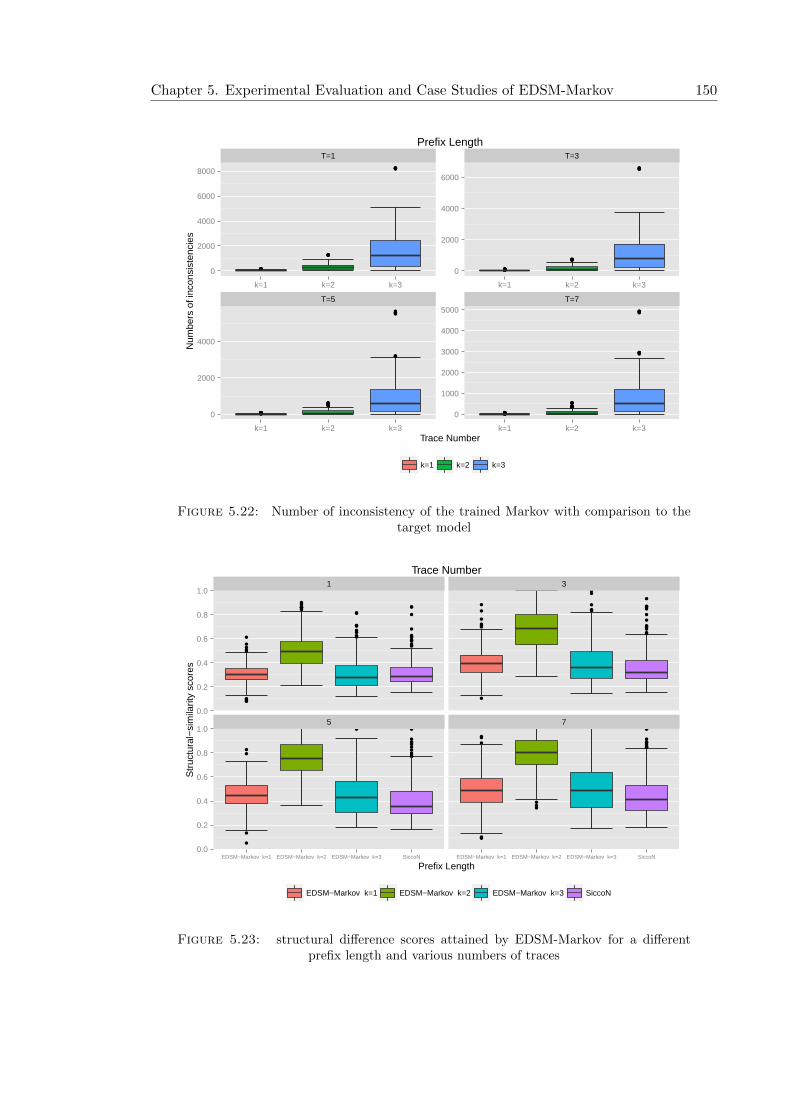
Chapter 5. Experimental Evaluation and Case Studies of EDSM-Markov 150
T=1 T=3
T=5 T=7
0
2000
4000
6000
8000
0
2000
4000
6000
0
2000
4000
0
1000
2000
3000
4000
5000
k=1 k=2 k=3 k=1 k=2 k=3
k=1 k=2 k=3 k=1 k=2 k=3Trace Number
Num
bers
of i
ncon
sist
enci
es
k=1 k=2 k=3
Prefix Length
Figure 5.22: Number of inconsistency of the trained Markov with comparison to thetarget model
1 3
5 70.0
0.2
0.4
0.6
0.8
1.0
0.0
0.2
0.4
0.6
0.8
1.0
EDSM−Markov k=1 EDSM−Markov k=2 EDSM−Markov k=3 SiccoN EDSM−Markov k=1 EDSM−Markov k=2 EDSM−Markov k=3 SiccoN
Prefix Length
Str
uctu
ral−
sim
ilarit
y sc
ores
EDSM−Markov k=1 EDSM−Markov k=2 EDSM−Markov k=3 SiccoN
Trace Number
Figure 5.23: structural difference scores attained by EDSM-Markov for a differentprefix length and various numbers of traces

Chapter 5. Experimental Evaluation and Case Studies of EDSM-Markov 151
BCR scores obtained by EDSM-Markov are higher than those obtained using SiccoN in
the majority of random LTSs used in the experiments.
K T
p-value of
E-M Vs.SiccoNMean BCR
Mean
structural similarity
BCR Structural similarity E-M SiccoN E-M SiccoN
1
1 4.47× 10−07 0.34 0.58 0.56 0.31 0.31
3 9.77× 10⁻²⁰ 1.62× 10−08 0.79 0.71 0.40 0.35
5 2.82× 10⁻¹⁴ 1.52× 10−07 0.86 0.80 0.45 0.41
7 6.02× 10−08 6.98× 10−06 0.89 0.86 0.49 0.45
2
1 4.49× 10−07 4.40× 10−46 0.58 0.56 0.50 0.31
3 7.33× 10−40 2.38× 10−49 0.85 0.71 0.68 0.35
5 1.97× 10−43 3.76× 10−49 0.93 0.80 0.76 0.41
7 2.09× 10−39 2.07× 10−49 0.96 0.86 0.80 0.45
3
1 4.60× 10−08 0.34 0.54 0.56 0.31 0.31
3 0.003 4.93× 10−07 0.69 0.71 0.40 0.35
5 0.26 1.72× 10−08 0.80 0.80 0.45 0.41
7 0.97 4.93× 10⁻¹² 0.86 0.86 0.52 0.45
Table 5.7: p-values obtained using the Wilcoxon signed rank test for different prefixlength
Additionally, the fourth column in Table 5.7 summarizes the statistical test results using
the Wilcoxon signed-rank test for structural-similarity scores. The obtained p-values are
below 0.05 in the majority settings of K. Hence, the null hypothesis can be rejected. This
proves that the structural-similarity scores of the inferred LTSs using EDSM-Markov are
higher than those obtained using SiccoN. Furthermore, the null hypothesis is accepted
when the number of traces is one and k = 1 or k = 3. This indicates that there is no
significant difference between the scores obtained using both learners.
5.3 Case Studies
In the previous section, the performance of the EDSM-Markov learner was evaluated
on randomly generated LTSs. In this section, the performance of EDSM-Markov was
evaluated on a number of case studies. For each of the following case studies, the number
of traces ranged from 1 to 8, and the length of traces was given by l ∗ |Q| ∗ |Σ|, where l
is a parameter to vary the length of generated traces. In the conducted experiment, 30
different random traces were generated. In addition, 2×|Q|2 test sequences were generated

Chapter 5. Experimental Evaluation and Case Studies of EDSM-Markov 152
of length 3×|Q|. This was chosen to match the settings used in the conducted experiments
using random LTSs.
5.3.1 Case Study: SSH Protocol
The first case study is the Secure Shell (SSH) protocol that is used for secure network
connect and login services [140]. Poll and Schubert [141] showed a formal state-machine
specification of SSH protocol that can be used for evaluating specification inference meth-
ods. In this case study, the number of states is 13 and alphabet size is 9, and number of
transitions is 17.
The outcomes that are shown in Figure 5.24 represent the BCR scores achieved using
different learners when l = 0.3, 0.5, and 1.0 respectively for the SSH case study. As can
be seen in Figure 5.24, the inferred LTSs using the EDSM-Markov learner are close to the
reference LTSs in terms of their language. The BCR scores increase whenever the number
of traces is increased and k = 2 or 3; this is because the Markov tables tend to be complete
and hence all labels of outgoing transitions that should be predicted are returned. It is
clear that the EDSM-Markov learner performs badly when k = 1, especially if the number
of traces is 4 or 8. In addition, in terms of language comparison, SiccoN inferred better
LTSs compared to the EDSM-Markov k = 1 learner.
lTrace Number
1 2 4 8
0.3
EDSM-Markov k=1 vs. SiccoN 0.015 0.01 0.64 4.04× 10−05
EDSM-Markov k=2 vs. SiccoN 0.002 0.002 1.82× 10−06 2.63× 10−05
EDSM-Markov k=3 vs. SiccoN 0.74 0.005 9.75× 10−06 2.27× 10−05
0.5
EDSM-Markov k=1 vs. SiccoN 0.01 0.05 0.31 0.001
EDSM-Markov k=2 vs. SiccoN 3.48× 10−04 1.02× 10−05 3.01× 10−06 1.76× 10−06
EDSM-Markov k=3 vs. SiccoN 0.002 3.04× 10−04 4.04× 10−06 1.56× 10−06
1.0
EDSM-Markov k=1 vs. SiccoN 0.35 0.05 0.76 3.60× 10−06
EDSM-Markov k=2 vs. SiccoN 3.98× 10−06 1.60× 10−04 2.73× 10−06 1.72× 10−06
EDSM-Markov k=3 vs. SiccoN 6.31× 10−05 1.01× 10−04 1.99× 10−06 1.80× 10−06
Table 5.8: p-values obtained using the Wilcoxon signed-rank test of SSH protocol casestudy for BCR scores
Table 5.8 summarizes the resulting p-values from the Wilcoxon signed-rank statistical test
for the BCR scores attained by learners. The null hypothesis H0 states that the BCR scores

Chapter 5. Experimental Evaluation and Case Studies of EDSM-Markov 153
1 2
4 80.4
0.5
0.6
0.7
0.8
0.9
1.0
0.4
0.5
0.6
0.7
0.8
0.9
1.0
l=0.3 l=0.5 l=1.0 l=0.3 l=0.5 l=1.0Trace Length Muliplier
BC
R s
core
EDSM−Markov k =1 EDSM−Markov k =2 EDSM−Markov k =3 SiccoN
Trace Number
Figure 5.24: BCR scores of SSH Protocol case study
obtained by EDSM-Markov and SiccoN are the same. The p-values suggest rejection of
the H0 when the number of traces is larger than 2 and k > 1; because the p-values are less
than 0.05, indicating that there is a statistically significant difference between them. As
mentioned in Table 5.8, when comparing EDSM-Markov k=1 and SiccoN, the H0 can be
accepted when the number of traces is 4. This indicates there is no significant difference
between both learners.
The evaluation of EDSM-Markov using random LTSs in Section 5.2 was shown to signifi-
cantly improve the structural-similarity scores of the inferred LTSs. In the SSH case study,
the structural-similarity scores obtained by EDSM-Markov when k = 2 and 3 were higher
than those obtained by SiccoN as shown in Figure 5.25. The low values of the structural-
similarity scores of LTSs inferred using SiccoN means that the synthesized LTSs had extra
transitions that should be removed. In addition, the structural-similarity scores attained
by the EDSM-Markov learner when k = 1 are worse than other learners. This contributed
to the low precision scores of the trained Markov model whereas many inconsistencies
are not detected by the EDSM-Markov k = 1 learner. Hence, it is obvious that SiccoN
generated LTSs better than EDSM-Markov if k = 1. The reason behind this is that when-
ever the EDSM-Markov k = 1 learner merged a pair of states, new labels of the outgoing
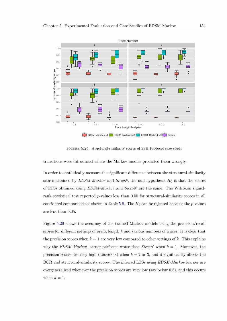
Chapter 5. Experimental Evaluation and Case Studies of EDSM-Markov 154
1 2
4 80.0
0.2
0.4
0.6
0.8
1.0
0.0
0.2
0.4
0.6
0.8
1.0
l=0.3 l=0.5 l=1.0 l=0.3 l=0.5 l=1.0Trace Length Muliplier
stru
ctur
al s
imila
rity
scor
e
EDSM−Markov k =1 EDSM−Markov k =2 EDSM−Markov k =3 SiccoN
Trace Number
Figure 5.25: structural-similarity scores of SSH Protocol case study
transitions were introduced where the Markov models predicted them wrongly.
In order to statistically measure the significant difference between the structural-similarity
scores attained by EDSM-Markov and SiccoN, the null hypothesis H0 is that the scores
of LTSs obtained using EDSM-Markov and SiccoN are the same. The Wilcoxon signed-
rank statistical test reported p-values less than 0.05 for structural-similarity scores in all
considered comparisons as shown in Table 5.9. The H0 can be rejected because the p-values
are less than 0.05.
Figure 5.26 shows the accuracy of the trained Markov models using the precision/recall
scores for different settings of prefix length k and various numbers of traces. It is clear that
the precision scores when k = 1 are very low compared to other settings of k. This explains
why the EDSM-Markov learner performs worse than SiccoN when k = 1. Moreover, the
precision scores are very high (above 0.8) when k = 2 or 3, and it significantly affects the
BCR and structural-similarity scores. The inferred LTSs using EDSM-Markov learner are
overgeneralized whenever the precision scores are very low (say below 0.5), and this occurs
when k = 1.
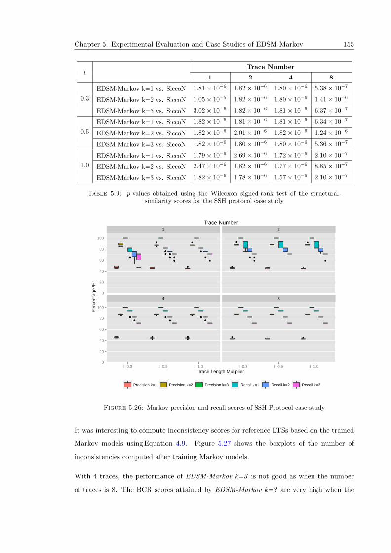
Chapter 5. Experimental Evaluation and Case Studies of EDSM-Markov 155
lTrace Number
1 2 4 8
0.3
EDSM-Markov k=1 vs. SiccoN 1.81× 10⁻⁶ 1.82× 10⁻⁶ 1.80× 10⁻⁶ 5.38× 10⁻⁷
EDSM-Markov k=2 vs. SiccoN 1.05× 10⁻⁵ 1.82× 10⁻⁶ 1.80× 10⁻⁶ 1.41× 10⁻⁶
EDSM-Markov k=3 vs. SiccoN 3.02× 10⁻⁶ 1.82× 10⁻⁶ 1.81× 10⁻⁶ 6.37× 10⁻⁷
0.5
EDSM-Markov k=1 vs. SiccoN 1.82× 10⁻⁶ 1.81× 10⁻⁶ 1.81× 10⁻⁶ 6.34× 10⁻⁷
EDSM-Markov k=2 vs. SiccoN 1.82× 10⁻⁶ 2.01× 10⁻⁶ 1.82× 10⁻⁶ 1.24× 10⁻⁶
EDSM-Markov k=3 vs. SiccoN 1.82× 10⁻⁶ 1.80× 10⁻⁶ 1.80× 10⁻⁶ 5.36× 10⁻⁷
1.0
EDSM-Markov k=1 vs. SiccoN 1.79× 10⁻⁶ 2.69× 10⁻⁶ 1.72× 10⁻⁶ 2.10× 10⁻⁷
EDSM-Markov k=2 vs. SiccoN 2.47× 10⁻⁶ 1.82× 10⁻⁶ 1.77× 10⁻⁶ 8.85× 10⁻⁷
EDSM-Markov k=3 vs. SiccoN 1.82× 10⁻⁶ 1.78× 10⁻⁶ 1.57× 10⁻⁶ 2.10× 10⁻⁷
Table 5.9: p-values obtained using the Wilcoxon signed-rank test of the structural-similarity scores for the SSH protocol case study
1 2
4 80
20
40
60
80
100
0
20
40
60
80
100
l=0.3 l=0.5 l=1.0 l=0.3 l=0.5 l=1.0Trace Length Muliplier
Per
cent
age
%
Precision k=1 Precision k=2 Precision k=3 Recall k=1 Recall k=2 Recall k=3
Trace Number
Figure 5.26: Markov precision and recall scores of SSH Protocol case study
It was interesting to compute inconsistency scores for reference LTSs based on the trained
Markov models using Equation 4.9. Figure 5.27 shows the boxplots of the number of
inconsistencies computed after training Markov models.
With 4 traces, the performance of EDSM-Markov k=3 is not good as when the number
of traces is 8. The BCR scores attained by EDSM-Markov k=3 are very high when the

Chapter 5. Experimental Evaluation and Case Studies of EDSM-Markov 156
1 2
4 80
4
8
12
16
20
24
28
0
4
8
12
16
20
24
28
l=0.3 l=0.5 l=1.0 l=0.3 l=0.5 l=1.0Trace Length Muliplier
Num
ber
of in
cons
iste
ncie
s
Markov k =1 Markov k =2 Markov k =3
Trace Number
Figure 5.27: Inconsistencies of SSH protocol case study
number of traces is 4 or 8. This is because the number of inconsistencies computed for
reference graphs was below 10. The number of inconsistencies was very high when k = 3
and the number of traces is 1 and 2, denoting that Markov models need to have extra
training data to visit states using different paths in order to get higher BCR scores.
There is a relationship between the number of inconsistencies in reference graphs and the
quality of the inferred LTS models. Generally, a very high inconsistency score means that
a Markov table does not train well with respect to subsequences of events of length k+ 1.

Chapter 5. Experimental Evaluation and Case Studies of EDSM-Markov 157
5.3.2 Case Study: Mine Pump
The second case study is the mine pump system that is introduced by Damas et al. [142]
for the following requirement: the pump must be switched off whenever the water level
is below a low threshold. Damas et al. [142] showed a simplified LTS specification of mine
pump that can be used for evaluating LTS inference methods. In this case study, the
number of states is 10, alphabet size is 8, and the number of transitions is 13.
1 2
4 80.4
0.5
0.6
0.7
0.8
0.9
1.0
0.4
0.5
0.6
0.7
0.8
0.9
1.0
L=0.3 L=0.5 L=1.0 L=0.3 L=0.5 L=1.0Trace Length Muliplier
BC
R s
core
EDSM−Markov k =1 EDSM−Markov k =2 EDSM−Markov k =3 SiccoN
Trace Number
Figure 5.28: BCR scores of water mine pump case study
Figure 5.28 illustrates the BCR scores of the inferred LTSs for the mine pump case study
using EDSM-Markov and SiccoN, where different numbers of traces were considered. It is
obvious from Figure 5.28 that the EDSM-Markov learner inferred LTSs with higher BCR
scores in the majority of cases, especially when the number of traces was higher than 1 and
k > 1. The EDSM-Markov k = 1 learner did not learn LTSs well compared to SiccoN if the
number of traces was 4 or 8. This was because the accuracy of the trained Markov model
when k = 1 was not good compared to k = 2 or k = 3. It is apparent from Figure 5.28
that the SiccoN learner performs well on heavily-branching traces compared to the EDSM-
Markov learner when k = 1. It is interesting to note that EDSM-Markov k=2 and EDSM-
Markov k=3 learners inferred LTSs with BCR scores much higher than those obtained

Chapter 5. Experimental Evaluation and Case Studies of EDSM-Markov 158
using SiccoN even if there are 1 or 2 traces considered. This indicates that the trained
Markov models predicted labels of outgoing transitions well during the process of merging
states.
Additionally, SiccoN performed well when the number of traces was 8, in contrast to when
it was 1 or 2. This is because SiccoN is going to infer LTSs well whenever the traces are
heavily branched, and this interprets why SiccoN generates LTSs of the mine pump case
study with BCR scores close to those inferred by EDSM-Markov k=2 and EDSM-Markov
k=3.
Table 5.10 shows the reported p-values of BCR scores obtained from the Wilcoxon signed-
rank statistical test. The null hypothesis H0 is that there is no significant difference
between the BCR scores of the inferred LTS using EDSM-Markov and SiccoN. The result-
ing p-values were less than 0.05. Therefore, the H0 could be rejected. It is clear that there
was a significant difference between SiccoN and EDSM-Markov when k = 1 if the number
of traces was 8, indicating that SiccoN performed better than EDSM-Markov k=1. On
the other hand, the null hypothesis was accepted if the number of traces was 4, denoting
that there was no significant difference between SiccoN and EDSM-Markov k=1.
lTrace Number
1 2 4 8
0.3
EDSM-Markov k=1 vs. SiccoN 0.52 0.03 0.75 2.18× 10−05
EDSM-Markov k=2 vs. SiccoN 0.06 0.002 7.33× 10−04 9.55× 10−07
EDSM-Markov k=3 vs. SiccoN 0.017 8.40× 10−04 0.003 9.55× 10−07
0.5
EDSM-Markov k=1 vs. SiccoN 0.002 5.82× 10−04 0.40 7.76× 10−04
EDSM-Markov k=2 vs. SiccoN 0.003 2.58× 10−05 5.33× 10−05 1.16× 10−06
EDSM-Markov k=3 vs. SiccoN 0.06 0.003 7.08× 10−05 1.16× 10−06
1.0
EDSM-Markov k=1 vs. SiccoN 0.003 0.024 0.39 2.98× 10−05
EDSM-Markov k=2 vs. SiccoN 2.13× 10−04 5.03× 10−05 2.60× 10−06 1.14× 10−06
EDSM-Markov k=3 vs. SiccoN 1.29× 10−04 1.81× 10−06 2.58× 10−06 1.14× 10−06
Table 5.10: p-values of Wilcoxon signed rank test of water mine case study for BCRscores
Figure 5.29 shows the structural-similarity scores of the mined LTSs for the water mine
pump case study. The outcomes that are shown in Figure 5.29 support the hypothesis
that EDSM-Markov generates LTSs models that are structurally very similar to the ref-
erence LTS compared to those models inferred using SiccoN when k = 2 and 3. The
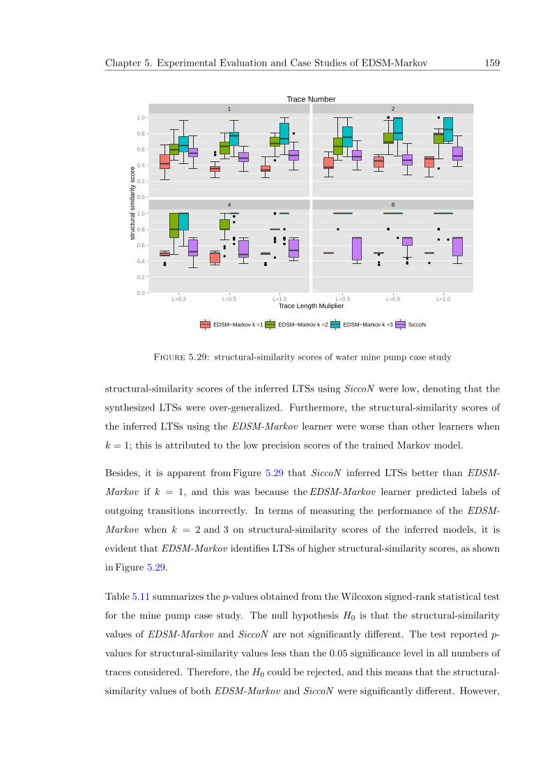
Chapter 5. Experimental Evaluation and Case Studies of EDSM-Markov 159
1 2
4 80.0
0.2
0.4
0.6
0.8
1.0
0.0
0.2
0.4
0.6
0.8
1.0
L=0.3 L=0.5 L=1.0 L=0.3 L=0.5 L=1.0Trace Length Muliplier
stru
ctur
al s
imila
rity
scor
e
EDSM−Markov k =1 EDSM−Markov k =2 EDSM−Markov k =3 SiccoN
Trace Number
Figure 5.29: structural-similarity scores of water mine pump case study
structural-similarity scores of the inferred LTSs using SiccoN were low, denoting that the
synthesized LTSs were over-generalized. Furthermore, the structural-similarity scores of
the inferred LTSs using the EDSM-Markov learner were worse than other learners when
k = 1; this is attributed to the low precision scores of the trained Markov model.
Besides, it is apparent from Figure 5.29 that SiccoN inferred LTSs better than EDSM-
Markov if k = 1, and this was because the EDSM-Markov learner predicted labels of
outgoing transitions incorrectly. In terms of measuring the performance of the EDSM-
Markov when k = 2 and 3 on structural-similarity scores of the inferred models, it is
evident that EDSM-Markov identifies LTSs of higher structural-similarity scores, as shown
in Figure 5.29.
Table 5.11 summarizes the p-values obtained from the Wilcoxon signed-rank statistical test
for the mine pump case study. The null hypothesis H0 is that the structural-similarity
values of EDSM-Markov and SiccoN are not significantly different. The test reported p-
values for structural-similarity values less than the 0.05 significance level in all numbers of
traces considered. Therefore, the H0 could be rejected, and this means that the structural-
similarity values of both EDSM-Markov and SiccoN were significantly different. However,

Chapter 5. Experimental Evaluation and Case Studies of EDSM-Markov 160
the H0 was accepted if the number of traces was 2 and l = 0.5 when the structural-
similarity scores for the mined LTSs using EDSM-Markov k=1 were compared to the scores
attained by SiccoN, and this suggested that there was no significant difference between the
structural-similarity scores.
lTrace Number
1 2 4 8
0.3
EDSM-Markov k=1 vs. SiccoN 1.25× 10−05 1.04× 10−04 0.004 1.78× 10−04
EDSM-Markov k=2 vs. SiccoN 0.04 3.09× 10−04 1.79× 10−06 1.03× 10−06
EDSM-Markov k=3 vs. SiccoN 0.001 1.16× 10−05 1.78× 10−06 1.03× 10−06
0.5
EDSM-Markov k=1 vs. SiccoN 1.13× 10−05 0.10 0.01 1.52× 10−05
EDSM-Markov k=2 vs. SiccoN 3.40× 10−05 1.82× 10−06 1.80× 10−06 1.17× 10−06
EDSM-Markov k=3 vs. SiccoN 1.17× 10−05 2.47× 10−06 1.80× 10−06 1.17× 10−06
1.0
EDSM-Markov k=1 vs. SiccoN 1.53× 10−05 1.91× 10−04 0.002 8.12× 10−05
EDSM-Markov k=2 vs. SiccoN 1.07× 10−05 7.97× 10−06 1.77× 10−06 1.16× 10−06
EDSM-Markov k=3 vs. SiccoN 4.00× 10−06 1.81× 10−06 1.77× 10−06 1.16× 10−06
Table 5.11: p-values of Wilcoxon signed rank test of water mine case study for structural-similarity Scores
The precision and recall scores of the Markov models were computed during the conducted
experiments. The intention behind computing this is to study the influence of Markov
models on the accuracy of the inferred LTSs. Figure 5.30 illustrates the precision/recall
scores of the trained Markov models for different settings of prefix length k, and a varied
number of traces were considered. It can be seen from Figure 5.30 that the precision scores
of the trained Markov models when k = 1 were very low compared to other settings of
k, and this explains why the EDSM-Markov learner performed worse than SiccoN when
k = 1. The EDSM-Markov learner over-generalized whenever the precision score was very
low (say below 0.5), and this happened if k = 1. It is noticed that the precision scores
were very high (above 0.8) when k = 2 or 3 and it had a significantly positive effect on
the BCR and structural-similarity scores.
Figure 5.31 shows the number of inconsistencies computed for the reference LTS of the
water mine case study after training Markov models. In case where k = 3, the mean value
of the BCR scores of the inferred LTSs using EDSM-Markov was higher than (say 0.95)
when the number of traces was 4 or 8. This can be attributed to the low inconsistency
score in this case, as shown in Figure 5.31. In contrast, low BCR scores of the inferred
LTSs using EDSM-Markov were achieved if the number of traces was very small and k = 3;

Chapter 5. Experimental Evaluation and Case Studies of EDSM-Markov 161
1 2
4 80
20
40
60
80
100
0
20
40
60
80
100
L=0.3 L=0.5 L=1.0 L=0.3 L=0.5 L=1.0Trace Length Muliplier
Per
cent
age
%
Precision k=1 Precision k=2 Precision k=3 Recall k=1 Recall k=2 Recall k=3
Trace Number
Figure 5.30: Markov precision and recall scores of water mine case study
this indicates that Markov models did not train well to observe sequences of length k+ 1.
5.3.3 Case Study: CVS Client
The third case study is concurrent versions system (CVS) protocol that is proposed by Lo
and cheng Khoo [143]. They used it to evaluate their state machine inference approach.
The functionalities of CVS implementation are incorporated with the FTP package that is
included by Jakarta Commons Net library [143]. In this case study, the number of states
is 15, and the alphabet size is 15, and the number of transitions is 27.
The BCR results of LTSs that were inferred using the considered miners are shown
in Figure 5.32. It is interesting to note that EDSM-Markov k=1 inferred LTSs with bet-
ter BCR scores compared to other learners if the number of traces was 1 or 2. Moreover,
the EDSM-Markov k=3 performed badly since Markov models did not train well and many
labels of outgoing transitions were miss-predicted after merging states, which resulted in
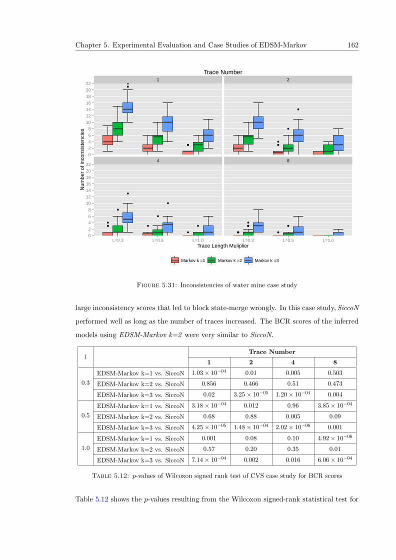
Chapter 5. Experimental Evaluation and Case Studies of EDSM-Markov 162
1 2
4 80
2
4
6
8
10
12
14
16
18
20
22
0
2
4
6
8
10
12
14
16
18
20
22
L=0.3 L=0.5 L=1.0 L=0.3 L=0.5 L=1.0Trace Length Muliplier
Num
ber
of in
cons
iste
ncie
s
Markov k =1 Markov k =2 Markov k =3
Trace Number
Figure 5.31: Inconsistencies of water mine case study
large inconsistency scores that led to block state-merge wrongly. In this case study, SiccoN
performed well as long as the number of traces increased. The BCR scores of the inferred
models using EDSM-Markov k=2 were very similar to SiccoN.
lTrace Number
1 2 4 8
0.3
EDSM-Markov k=1 vs. SiccoN 1.03× 10−04 0.01 0.005 0.503
EDSM-Markov k=2 vs. SiccoN 0.856 0.466 0.51 0.473
EDSM-Markov k=3 vs. SiccoN 0.02 3.25× 10−05 1.20× 10−04 0.004
0.5
EDSM-Markov k=1 vs. SiccoN 3.18× 10−04 0.012 0.96 3.85× 10−04
EDSM-Markov k=2 vs. SiccoN 0.68 0.88 0.005 0.09
EDSM-Markov k=3 vs. SiccoN 4.25× 10−05 1.48× 10−04 2.02× 10−06 0.001
1.0
EDSM-Markov k=1 vs. SiccoN 0.001 0.08 0.10 4.92× 10−06
EDSM-Markov k=2 vs. SiccoN 0.57 0.20 0.35 0.01
EDSM-Markov k=3 vs. SiccoN 7.14× 10−04 0.002 0.016 6.06× 10−04
Table 5.12: p-values of Wilcoxon signed rank test of CVS case study for BCR scores
Table 5.12 shows the p-values resulting from the Wilcoxon signed-rank statistical test for

Chapter 5. Experimental Evaluation and Case Studies of EDSM-Markov 163
1 2
4 80.4
0.5
0.6
0.7
0.8
0.9
1.0
0.4
0.5
0.6
0.7
0.8
0.9
1.0
L=0.3 L=0.5 L=1.0 L=0.3 L=0.5 L=1.0Trace Length Muliplier
BC
R s
core
EDSM−Markov k =1 EDSM−Markov k =2 EDSM−Markov k =3 SiccoN
Trace Number
Figure 5.32: BCR scores of CVS protocol case study
BCR scores. The null hypothesis H0 is that the BCR scores of EDSM-Markov and SiccoN
are the same. The resulting p-values obtained by comparing the BCR scores of EDSM-
Markov learners and SiccoN were larger than 0.05, so the H0 could be accepted as shown
in Table 5.12. In cases where the p-value was higher than 0.5, it denotes that there was
no significant difference between learners. For instance, EDSM-Markov k=1 did not show
significant improvement when it compared with SiccoN in the case where the number of
traces was 8 and l = 0.3.
Figure 5.33 shows the structural-similarity scores of the inferred LTSs for CVS case study.
The findings that are shown in Figure 5.33 show that EDSM-Markov k=1 generated LTS
models with very low structural-similarity scores compared to other learners. This is
because EDSM-Markov k=1 inferred over-generalized LTSs. In addition, the structural-
similarity scores of the inferred LTSs using the EDSM-Markov learner when k = 1 were

Chapter 5. Experimental Evaluation and Case Studies of EDSM-Markov 164
1 2
4 80.0
0.2
0.4
0.6
0.8
1.0
0.0
0.2
0.4
0.6
0.8
1.0
L=0.3 L=0.5 L=1.0 L=0.3 L=0.5 L=1.0Trace Length Muliplier
stru
ctur
al s
imila
rity
scor
e
EDSM−Markov k =1 EDSM−Markov k =2 EDSM−Markov k =3 SiccoN
Trace Number
Figure 5.33: Structural-similarity scores of CVS protocol case study
worse than other learners. It is clear from Figure 5.33 that SiccoN inferred LTSs better
than EDSM-Markov if k = 1. This was because the EDSM-Markov learner predicted
labels of outgoing transitions incorrectly. Moreover, the structural-similarity scores of the
inferred models EDSM-Markov learner when k = 2 and 3 were higher than SiccoN in some
cases, especially when the number of traces was 1 or 2, as shown in Figure 5.33.
Figure 5.34 illustrates the precision/recall scores of the trained Markov models for CVS
case study. It is clear from Figure 5.34 that the precision scores of the trained Markov
models were very high in all settings of k. This may explain why the EDSM-Markov
learner generated LTSs with high BCR scores when k = 1.
Figure 5.35 shows the number of inconsistencies computed for the reference LTS of CVS
case study after training Markov models. In general, a very low inconsistency score means
that a Markov table does not train well with respect to subsequences of length k+ 1. One

Chapter 5. Experimental Evaluation and Case Studies of EDSM-Markov 165
lTrace Number
1 2 4 8
0.3
EDSM-Markov k=1 vs. SiccoN 6.93× 10−05 1.42× 10−04 2.97× 10−05 1.82× 10−06
EDSM-Markov k=2 vs. SiccoN 0.001 9.22× 10−06 0.04 0.047
EDSM-Markov k=3 vs. SiccoN 0.008 0.134 0.018 0.21
0.5
EDSM-Markov k=1 vs. SiccoN 1.68× 10−06 6.15× 10−08 2.61× 10−08 1.86× 10−09
EDSM-Markov k=2 vs. SiccoN 0.001 0.003 0.114 0.59
EDSM-Markov k=3 vs. SiccoN 0.35 0.10 0.90 0.55
1.0
EDSM-Markov k=1 vs. SiccoN 1.22× 10−05 2.61× 10−08 3.73× 10−09 1.82× 10−06
EDSM-Markov k=2 vs. SiccoN 4.97× 10−05 0.01 0.39 0.87
EDSM-Markov k=3 vs. SiccoN 0.001 0.04 0.83 0.58
Table 5.13: p-values of Wilcoxon signed rank test of CVS case study for structural-similarity scores
1 2
4 80
20
40
60
80
100
0
20
40
60
80
100
L=0.3 L=0.5 L=1.0 L=0.3 L=0.5 L=1.0Trace Length Muliplier
Per
cent
age
%
Precision k=1 Precision k=2 Precision k=3 Recall k=1 Recall k=2 Recall k=3
Trace Number
Figure 5.34: Markov precision and recall scores of water mine case study
can observe that when k = 3, the mean value of the BCR scores for the inferred LTSs using
EDSM-Markov was below 0.95, for example, in the majority cases, except when l = 1.0
and the number of traces was 8; low BCR scores of the learnt LTSs when k = 3 is due to
that the number of inconsistencies were very high.

Chapter 5. Experimental Evaluation and Case Studies of EDSM-Markov 166
1 2
4 805
101520253035404550556065
05
101520253035404550556065
L=0.3 L=0.5 L=1.0 L=0.3 L=0.5 L=1.0Trace Length Muliplier
Num
ber
of in
cons
iste
ncie
s
Markov k =1 Markov k =2 Markov k =3
Trace Number
Figure 5.35: Inconsistencies of CVS case study

Chapter 5. Experimental Evaluation and Case Studies of EDSM-Markov 167
5.4 Discussion
As mentioned in the introduction chapter, one of the aims in this thesis is to improve the
existing techniques to tackle the over-generalization problem. In this chapter, experimental
assessment of the performance of EDSM-Markov has been achieved using random LTSs
and case studies. The performance of EDSM-Markov has been studied from different
aspects.
In Section 5.2, different questions were introduced in order to answer them after evaluating
the performance of the proposed learner. The first question is about the effect of the
number of traces on the performance of EDSM-Markov. The findings obtained from the
conduced experiments based on both random LTSs and case studies demonstrate that
the efficiency of the EDSM-Markov learner can be improved while the number of traces
increases. This is intuitive because the quality of the inferred state machine models depend
on the number of the provided traces, as stated by Walkinshaw and Bogdanov [77]. With
respect to our findings, EDSM-Markov fails to generalize LTSs well if the provided traces
are insufficient.
Another important finding is that EDSM-Markov improves the accuracy of the inferred
LTSs when the alphabet size are very large. This is because Markov precisions tend to be
high in such settings and this helps to make correct mergers during the inference process.
The results from the conducted experiments using the random LTSs demonstrate that
with few long traces available, the Markov-EDSM learner can improve the accuracy of the
inferred LTSs with large alphabets. This addresses the research question that concerned
about how well EDSM-Markov infers LTSs with large alphabets.
One of the more significant findings in this chapter is reasonable results were obtained if
the supplied traces were covered transitions in the reference LTSs well. Moreover, with
shorter traces provided, a poorer performance of the EDSM-Markov learner is expected
and this is because inferring the exact state-machine models from such traces are difficult.
It is important to highlight that the performance of EDSM-Markov are affected by the
setting of prefix length k. In the conducted experiments with random LTSs, EDSM-
Markov performed good when k = 2 compared to k = 3. The bad performance of EDSM-
Markov when k = 3 is because the provided traces are very sparse and Markov models
Chapter 5. Experimental Evaluation and Case Studies of EDSM-Markov 168
do not predict labels of outgoing transitions from a state to follow prefix paths of length
3. Surprisingly, for the water mine pump and ssh case studies, EDSM-Markov tends to
perform well if k = 3 and the number of traces is 8.
One interesting finding is that whenever the computed inconsistency scores for the refer-
ence LTSs after training the Markov models are too small, the EDSM-Markov learner can
infer reasonable LTSs on the condition that the precision scores of the trained Markov
models are high.
It was observed that EDSM-Markov learner performed better than SiccoN in the ma-
jority of cases. This is possibly due to the clever idea of EDSM-Markov that relies on
training Markov models and the IScore heuristic that, unlike SiccoN that blocks mergers.
Moreover, EDSM-Markov calculates an inconsistency score based on global view of depen-
dencies between events (elements of an alphabet) in the traces in order to block mergers,
and this differs from the way that SiccoN blocks mergers based on the local similarity of
labels of outgoing transitions.
Over-generalization is a known problem in the grammar inference domain. In their
study, Lo et al. [58] stated that the over-generalization during the inference of state ma-
chines should be controlled using the negative traces. However, the findings in this chapter
prove that EDSM-Markov can control the over-generalization. This is due to the idea of
inconsistencies that help EDSM-Markov to determine when a merger of states introduces
new labels of outgoing transitions that are prohibited to follow states based on Markov
predictions.
An approximate identification of state machines from sparsely training data is possible as
claimed by [113]. The EDSM-Markov learner has proven to generate good LTSs on the
condition that the alphabet size is very large.
To conclude, the conducted experiments agreed to the fact that the inference of automaton
from only positive traces is a difficult task. As stated by Chen and Rosu [144], the inference
of state-machine specification from positive traces is hard, it has been shown as a major
limitation of their works. In our study using random LTSs, a similar difficulty was observed
in the conducted experiments when few traces were provided and whenever the alphabet
size was |Σ| = 0.5× |Q|.

Chapter 5. Experimental Evaluation and Case Studies of EDSM-Markov 169
5.5 Threats to Validity
1. The randomly generated LTSs may not represent real-world models.
This threat is mitigated by evaluating the performance of EDSM-Markov on case
studies that are used in the literature review and the survey of stamina competi-
tion [35].
2. The selection of training data may not be representative .
One possible threat to validity is the selection of training data where they might not
berepresentative. For random LTSs, this threat is mitigated against it, each LTS was
attempted to infer 5 times with different paths generated each time since random
traces may follow the same paths many times. When the performance of EDSM-
Markov was evaluated on case studies, 30 different sets of random traces were used
in order to mitigate this threat.
3. The size of case studies may be limited. One possible threat to validity is that
the sizes of case studies are small. The performance of EDSM-Markov was evaluated
using case studies that are widely used in state machine inference papers. This threat
is mitigated by evaluating EDSM-Markov using random LTSs of different sizes.
4. The parameters settings may bias the results. In the conducted experiments,
there are many parameters such as the number and the length of traces, alphabet
size, and prefix length. Another potential threat to validity is that the variance
of such parameters may bias the results. This threat is mitigated by choosing a
different multiplier to vary the parameters. For instance, the length multiplier l was
introduced to assess the performance of EDSM-Markov on different length of traces.
Moreover, the alphabet multiplier m was chosen to vary the alphabet size to assess
the performance of EDSM-Markov on different types of LTSs.
5.6 Conclusions
The EDSM-Markov learner was proposed in the previous chapter, and it is a new method
of LTS inference using state merging based on computing inconsistencies scores from the
Markov models. This chapter evaluated the performance of the EDSM-Markov learner

Chapter 5. Experimental Evaluation and Case Studies of EDSM-Markov 170
from different dimensions such as the ability to infer LTSs from various lengths of traces
and sizes of alphabets. The purpose of the practical investigation was to determine the
effect of EDSM-Markov on solving the research problem, which is inferring LTSs from few
positive training data.
The evaluation of the performance of EDSM-Markov has demonstrated the capability to
improve upon SiccoN on the condition that the alphabet size is very large and the provided
traces cover transitions well.
The Markov learner that was proposed by Cook and Wolf [49] are not publicly available.
There is no information in the literature about the algorithm of the Markov learner.
Therefore, the comparison against their algorithm [49] are not difficult. Their ideas rely
on predictions using the first-order and second-order Markov models to build the event
graph. In the conducted experiments, the mean precision score of the second-order Markov
models was 65.6 when the number of traces was five. This showed that there is a kind
of over-generalisation in the inferred model using the Markov learner that was proposed
by Cook and Wolf [49]. However, the inferred models using EDSM-Markov prevents the
over-generalisation problem as shown in the earlier sections.

6Improvements to the QSM Algorithm
This chapter focuses on inferring LTS models from abstracted positive traces with the aid
of the active learning concept. In the previous chapter, the inference of LTS models using
passive methods was limited in some cases. This is due to the fact that passive techniques
require a high coverage of the system to infer LTS models well. This chapter presents
ModifiedQSM and MarkovQSM algorithms that are designed to infer LTS models from
positive training data using membership queries only. The basic idea behind this is to
improve the accuracy of the inferred LTSs using membership queries that are asked to
avoid bad state mergers.
6.1 Introduction
Passive LTSs inference from an incomplete set of samples cannot guarantee the generation
of complete models. This is because the prior set of samples may not cover every aspect of
171

Chapter 6. Improvements to the QSM Algorithm 172
the system under inference (learn), and this explains why passive techniques fail to infer
the exact models. Besides, collecting all requisite samples in advance to infer a correct
state machine can be expensive [100].
As stated in Chapter 3, active learning techniques of state machine models are very efficient
to accurately learn them. In the context of inferring LTS models from the samples, Dupont
et al. [36] showed that the idea of state-merging techniques can be integrated with the
concept of active learning. Thus, the QSM learner was developed by Dupont et al. [36].
It relies upon the provided samples that may not be characteristic and aims to infer the
exact models.
The QSM learner infers LTS models by asking membership queries to an oracle. The
submitted questions are considered as new samples (abstracted traces) that explore more
behaviours of the system under inference. Once the answers are obtained, the answered
queries are added to the initial collection of samples during the inference process. More-
over, the learning process is restarted whenever the answered query is contradicted with
the merged automaton.
The improvement that can be achieved by the QSM learner against passive state-merging
techniques is due to the fact that QSM asks queries to an oracle to gather information
about the language of the target LTSs. Furthermore, the queries that are asked during
the learning session of LTSs are aimed at preventing bad generalizations (merging non-
equivalent states in the hidden LTS model). Those queries extend the prior knowledge
about the behaviour of the system being learnt. Therefore, the answered queries are fed
again into the current automaton to explore how a system under inference behaves.
The performance of the QSM learner was studied earlier in this thesis in section 3.5, we
noticed that the accuracy of the learnt machines was not good enough if the alphabet
size was very large. In this chapter, we developed the ModifiedQSM and MarkovQSM
learners to improve the accuracy of the inferred LTSs. The performance of ModifiedQSM
and MarkovQSM were evaluated by a series of experiments using randomly generated
labelled-transition systems.

Chapter 6. Improvements to the QSM Algorithm 173
6.2 The Proposed Query Generators
In this section, the membership query generator of the ModifiedQSM and MarkovQSM
algorithms is described. It contains two sub-generators that are designed to work together
as one generator. The two sub-generators are described in Sections 6.2.1 and 6.2.2. The
following definitions are introduced before describing the generators of membership queries.
The set of sequences that lead to a state q from the initial state q0 is defined in Definition 6.1.
It is denoted by Seq (q).
Definition 6.1. Given a state q ∈ Q and the current automaton(A). Seq (q) = {w ∈
L(A)|δ(q0, w) = q}.
The shortest sequences that lead to a state q from the initial state q0 are defined in Definition 6.2,
denoted by Sp(q). The shortest sequences of the state Sp(q) are a subset of the short pre-
fixes of the language Sp(L) that is identified by the automaton A.
Definition 6.2. Given a state q ∈ Q, let Seq (q) denote the set of sequences that lead
to a state q from the initial state q0, and the current automaton(A). A sequence w
that belongs to the Seq (q) is said to be the shortest sequence if there is no other se-
quence y ∈ Seq (q) where the length of y is shorter than w. Sp(q) = {w ∈ Seq (q)|@y ∈
Seq (q)\{w} such that |w| > |y|}.
6.2.1 Dupont’s QSM Queries
The main generator of membership queries in the QSM algorithm was introduced by Dupont
et al. [36] and is called the Dupont generator in this thesis. The Dupont generator is re-
sponsible for the generation of queries about new scenarios (sequences) that appear as a
consequence of merging states. In other words, it is asked about sequences that belong to
the language of the merged automaton but do not belong to the language of the current
solution (LTS hypothesis). The objective of asking these queries is to prevent bad general-
izations (state merging) of the inferred models [36]. Hence, it is considered as an essential
(main) generator in ModifiedQSM and MarkovQSM.
Let Suff (qb, A) denotes the set of suffixes of the blue state qb in the current automaton(A).
The Dupont generator constructs the membership queries by first collecting the shortest

Chapter 6. Improvements to the QSM Algorithm 174
sequences that lead to the red state qr from the root state (q0) in A, denoted by Sp(qr).
The membership queries are generated by concatenating each sequence belonging to Sp(qr)
with each suffix belonging to Suff (qb, A) and not to Suff (qr, A). A generated membership
query is a sequence obtained by concatenating two sequences s · y such that s ∈ Sp(qr)
and y ∈ Suff (qb, A). Thus, the generated query s · y belongs to L(A′) and does not belong
to L(A). The way of constructing Dupont queries is defined in Definition 6.3.
Definition 6.3. Given a pair of red/blue states (qr, qb) ∈ Q, the current automaton(A),
and the merged automaton(A′). The Dupont queries is defined by:
Dupontqueries = {s · y | s ∈ Sp(qr), y ∈ Suff (qb, A)} such that s · y ∈ L(A′)\L(A).
The following two examples show how to construct the membership query for a recursive
and non-recursive merge of states respectively.
Astart B
C
D
G
E
H I
KLoad
Edit
Close
Edit
Save
Save Close
Load
(a) The current automaton A
Astart
C
D
G
E
H I
K
Load
Edit
Close
Edit
Save
Save Close
Load
(b) The merged automaton A′
Figure 6.1: The first example of computing the Dupontqueries
Example 6.1. Figure 6.1(a) shows the current automaton during the induction process.
Let us consider that the B state is chosen to merge with the A state. The shortest sequence
that leads to the red state A are empty, denoted by Sp(qr) = {ε}. The Suff (qb, A) set
contains the following sequences: {〈Edit, Edit, Save, Close〉, 〈Edit, Save〉, 〈Close, Load〉}.
The Dupontqueries queries are generated by concatenating the Sp(qr) with each suffix in
the Suff (qb, A) set as described in Definition 6.3. In this way, the following membership

Chapter 6. Improvements to the QSM Algorithm 175
queries are generated: Dupontqueries = {〈Edit, Edit, Save, Close〉, 〈Edit, Save〉, 〈Close,
Load〉}. It is clear that the generated queries belong to L(A′), which is shown in Fig-
ure 6.1(b), and do not belong to L(A).
Example 6.2. Figure 6.2(a) illustrates the current automaton during the inference pro-
cess. Consider that the G state is chosen to merge with the C state. Figure 6.2(a) shows
the merged automaton (A′) computed by merging the chosen pair of states. The short-
est sequence that leads to the red state C is Sp(qr) = 〈Load,Edit〉. The Suff (qb, A)
set contains the following sequences: {〈Save, Close〉}. The Dupontqueries queries are
generated by concatenating the Sp(qr) with each suffix in the Suff (qb, A) set as described
in Definition 6.3. In this way, the following membership queries are generated: Dupontqueries =
{〈Load,Edit, Save, Close〉}. It is noticed that the query belongs to L(A′) and does not
belong to L(A).
Astart B
C
D
G
E
H I
KLoad
Edit
Close
Edit
Save
Save Close
Load
(a) The current automaton A
Astart B
C
D
E I
KLoad
Edit
Close
Edit
Save Close
Load
(b) The merged automaton A′
Figure 6.2: The second example of computing the Dupontqueries
6.2.2 One-step Generator
The second generator of membership queries is called one-step. It is motivated by the
observation that the membership queries that are constructed using the Dupont generator
are insufficient to prevent merging inequivalent pairs of states. The example below shows
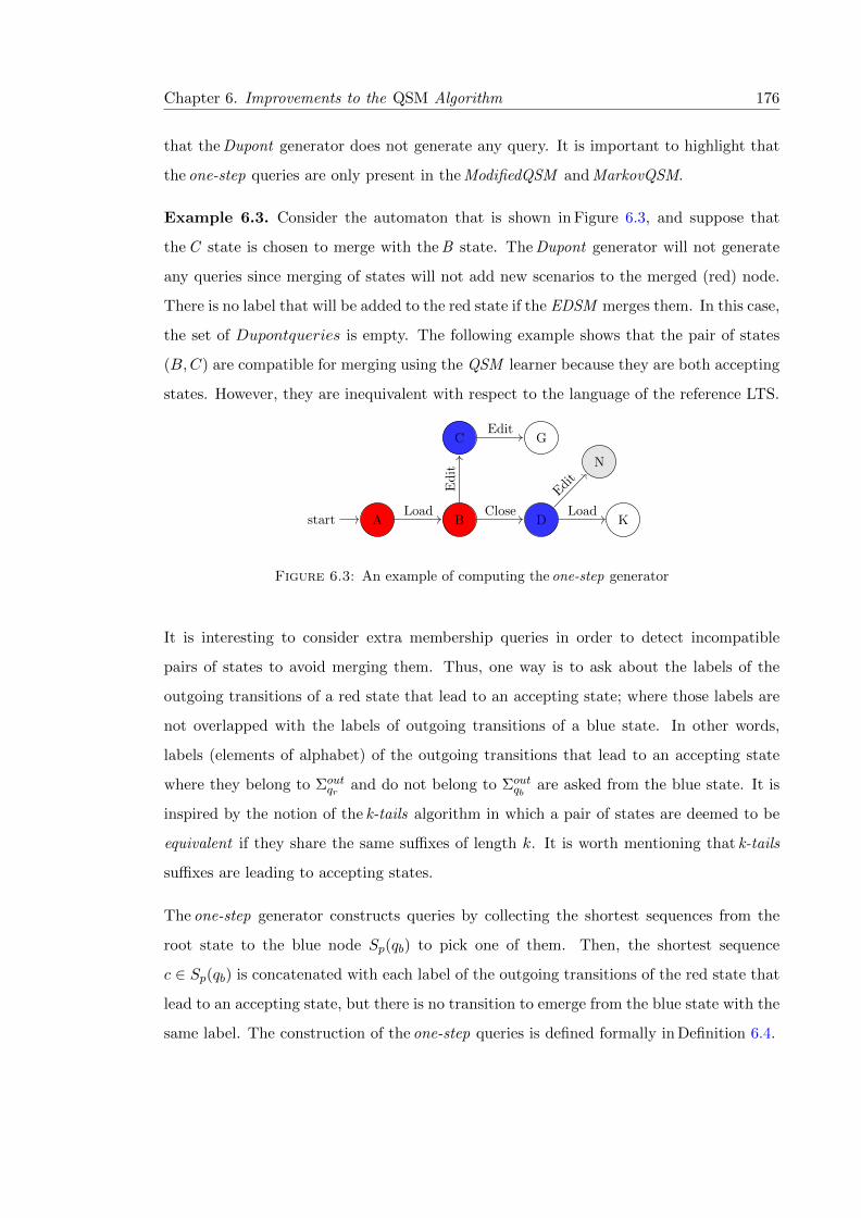
Chapter 6. Improvements to the QSM Algorithm 176
that the Dupont generator does not generate any query. It is important to highlight that
the one-step queries are only present in the ModifiedQSM and MarkovQSM.
Example 6.3. Consider the automaton that is shown in Figure 6.3, and suppose that
the C state is chosen to merge with the B state. The Dupont generator will not generate
any queries since merging of states will not add new scenarios to the merged (red) node.
There is no label that will be added to the red state if the EDSM merges them. In this case,
the set of Dupontqueries is empty. The following example shows that the pair of states
(B,C) are compatible for merging using the QSM learner because they are both accepting
states. However, they are inequivalent with respect to the language of the reference LTS.
Astart B
C
D
G
N
KLoad
Edit
Close
Edit
Edit
Load
Figure 6.3: An example of computing the one-step generator
It is interesting to consider extra membership queries in order to detect incompatible
pairs of states to avoid merging them. Thus, one way is to ask about the labels of the
outgoing transitions of a red state that lead to an accepting state; where those labels are
not overlapped with the labels of outgoing transitions of a blue state. In other words,
labels (elements of alphabet) of the outgoing transitions that lead to an accepting state
where they belong to Σoutqr and do not belong to Σout
qbare asked from the blue state. It is
inspired by the notion of the k-tails algorithm in which a pair of states are deemed to be
equivalent if they share the same suffixes of length k. It is worth mentioning that k-tails
suffixes are leading to accepting states.
The one-step generator constructs queries by collecting the shortest sequences from the
root state to the blue node Sp(qb) to pick one of them. Then, the shortest sequence
c ∈ Sp(qb) is concatenated with each label of the outgoing transitions of the red state that
lead to an accepting state, but there is no transition to emerge from the blue state with the
same label. The construction of the one-step queries is defined formally in Definition 6.4.
Chapter 6. Improvements to the QSM Algorithm 177
Definition 6.4. Given a pair of red/blue states (qr, qb) ∈ Q and the current automa-
ton(A). The one-step queries is defined by (oq) = {s · 〈σ〉 | s ∈ Sp(qb), σ ∈ Σoutqr \Σ
outqb∧ q′ ∈
δ(qr, σ) such that q′ ∈ F+}.
Example 6.4. Let us consider the pair of states that is shown in Figure 6.3 above, and
suppose that the C state is chosen to merge with the B state. The shortest path to the
blue state from the root state is Sp(C) = 〈Load,Edit〉. The Σoutqr \Σ
outqb
contains only
one label as follows: {Close}. In this example, the one-step generator results in only one
membership by concatenating Sp(C) with the Close label. This yields the following query:
onestep queries = {〈Load,Edit, Close〉}
6.3 The Modified QSM
In the original QSM [36], the RPNI learner computes a quotient automaton (Anew) that
is obtained by merging the chosen pair of states from the current automaton (A). After
that, the QSM algorithm asks membership queries about new scenarios that are consid-
ered new for A, but not for Anew. Dupont et al. [36] modified the strategy of selecting
pairs of states by adapting the EDSM and blue-fringe methods. In addition, the incorpo-
ration of the EDSM and blue-fringe methods in QSM leads to a reduction in the number
of membership queries consumed by QSM compared to the states-selection procedure us-
ing the RPNI learner [36]. The QSM is described in detail in chapter 3. In this section,
the ModifiedQSM algorithm is presented, and aims to tackle the large number of queries
produced by the QSM and increases the accuracy of the inferred LTS. In other words, it
aims to obtain better generalization of LTS compared to the QSM learner.
The ModifiedQSM is an adaptive algorithm of the EDSM learner and is designed to make
it an active learning. Membership queries are asked during the computation of the EDSM
score for possible pairs of states. The reason behind this is to detect incompatible pairs
of states and prevent merging them. In comparison with the original QSM, the benefit
of asking membership queries at that stage is that no restart of the learning process is
required. It differs from the original QSM that restarts learning an LTS model whenever
a membership query is answered as negative.
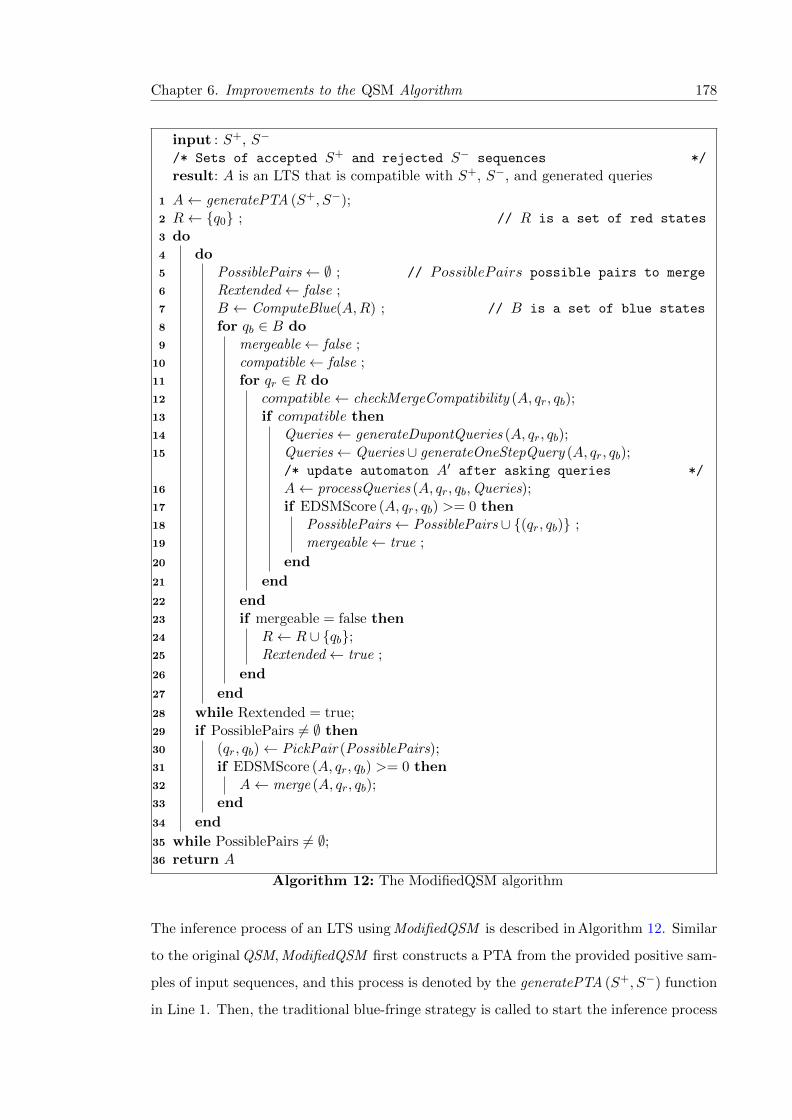
Chapter 6. Improvements to the QSM Algorithm 178
input : S+, S−
/* Sets of accepted S+ and rejected S− sequences */
result: A is an LTS that is compatible with S+, S−, and generated queries
1 A← generatePTA (S+, S−);2 R← {q0} ; // R is a set of red states
3 do4 do5 PossiblePairs← ∅ ; // PossiblePairs possible pairs to merge
6 Rextended← false ;7 B ← ComputeBlue(A,R) ; // B is a set of blue states
8 for qb ∈ B do9 mergeable← false ;
10 compatible← false ;11 for qr ∈ R do12 compatible← checkMergeCompatibility (A, qr, qb);13 if compatible then14 Queries← generateDupontQueries (A, qr, qb);15 Queries← Queries ∪ generateOneStepQuery (A, qr, qb);
/* update automaton A′ after asking queries */
16 A← processQueries (A, qr, qb,Queries);17 if EDSMScore (A, qr, qb) >= 0 then18 PossiblePairs← PossiblePairs ∪ {(qr, qb)} ;19 mergeable← true ;
20 end
21 end
22 end23 if mergeable = false then24 R← R ∪ {qb};25 Rextended← true ;
26 end
27 end
28 while Rextended = true;29 if PossiblePairs 6= ∅ then30 (qr, qb)← PickPair (PossiblePairs);31 if EDSMScore (A, qr, qb) >= 0 then32 A← merge (A, qr, qb);33 end
34 end
35 while PossiblePairs 6= ∅;36 return A
Algorithm 12: The ModifiedQSM algorithm
The inference process of an LTS using ModifiedQSM is described in Algorithm 12. Similar
to the original QSM, ModifiedQSM first constructs a PTA from the provided positive sam-
ples of input sequences, and this process is denoted by the generatePTA (S+, S−) function
in Line 1. Then, the traditional blue-fringe strategy is called to start the inference process
Chapter 6. Improvements to the QSM Algorithm 179
by colouring the root state red and all neighbouring states blue. The ComputeBlue(A,R)
function is called to colour the adjacent states of the red states blue.
The loop in Lines 8-27 is the selection of pairs of states in the ModifiedQSM algorithm based
on the blue-fringe strategy. It starts by iterating through the current blue B states in order
to evaluate their suitability for merging with the red states. Next, for each possible pair of
states, the compatibility of the pair is checked using the checkMergeCompatibility (A, r, b)
function as shown in Line 12. The pair of states (r, b) is said to be compatible if both states
are either accepting or rejecting. Moreover, the checkMergeCompatibility (A, r, b) function
checks the compatibility of states that would be merged recursively as well. If the pair of
states are incompatible, then no queries will be asked in this case. Otherwise, membership
queries are generated to avoid bad state merges.
The next stage is to construct membership queries in order to check the compatibility
of the pair of states based on queries to detect the incompatible ones and avoid merging
them. A list of membership queries is generated as described earlier in this chapter, and
this is denoted by the generateDupontQueries (A, r, b) and generateOneStepQuery (A, r, b)
functions.
Having generated a list of membership queries for a pair of states in Lines 14-15, the
processQueries (A, r, b,Queries) function is called to answer queries one by one b submit-
ting them to an oracle. Once a query is answered, it is added to the current automaton A,
and the compatibility of pairs is checked by computing the EDSM score. It is important
to say that the process of asking and answering queries can be terminated when the pair
of states is proven to be incompatible, even if there are remaining ones that have not been
answered yet. The process of answering membership queries is discussed in depth later
in Section 6.3.1. The pair of states is added to the PossiblePairs set if the EDSM score is
higher or equal to zero, denoting that the pair of states is compatible. The EDSM score is
computed for the current pair of states based on the updated automaton A′.
During the inference process, if the current blue state is mergeable with any red state, then
the pair (r, b) is added to the PossiblePairs set and the blue state is marked as mergeable.
For each blue state in the B set, it is promoted to red if it cannot merge with any of the
red states, and this is what EDSM does, as shown in Lines 23-26. The process is iterated
to colour the adjacent states of the red states blue.
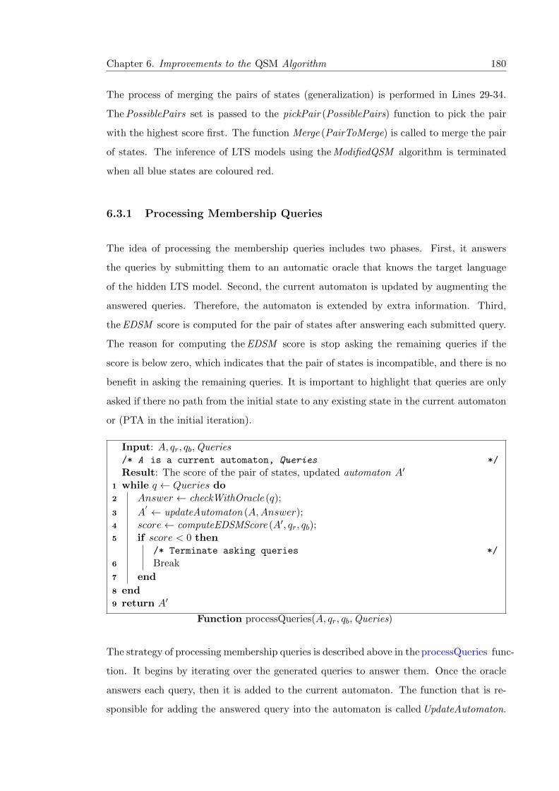
Chapter 6. Improvements to the QSM Algorithm 180
The process of merging the pairs of states (generalization) is performed in Lines 29-34.
The PossiblePairs set is passed to the pickPair (PossiblePairs) function to pick the pair
with the highest score first. The function Merge (PairToMerge) is called to merge the pair
of states. The inference of LTS models using the ModifiedQSM algorithm is terminated
when all blue states are coloured red.
6.3.1 Processing Membership Queries
The idea of processing the membership queries includes two phases. First, it answers
the queries by submitting them to an automatic oracle that knows the target language
of the hidden LTS model. Second, the current automaton is updated by augmenting the
answered queries. Therefore, the automaton is extended by extra information. Third,
the EDSM score is computed for the pair of states after answering each submitted query.
The reason for computing the EDSM score is stop asking the remaining queries if the
score is below zero, which indicates that the pair of states is incompatible, and there is no
benefit in asking the remaining queries. It is important to highlight that queries are only
asked if there no path from the initial state to any existing state in the current automaton
or (PTA in the initial iteration).
Input: A, qr, qb,Queries/* A is a current automaton, Queries */
Result: The score of the pair of states, updated automaton A′
1 while q ← Queries do2 Answer ← checkWithOracle (q);
3 A′ ← updateAutomaton (A,Answer);
4 score← computeEDSMScore (A′, qr, qb);5 if score < 0 then
/* Terminate asking queries */
6 Break
7 end
8 end9 return A′
Function processQueries(A, qr, qb,Queries)
The strategy of processing membership queries is described above in the processQueries func-
tion. It begins by iterating over the generated queries to answer them. Once the oracle
answers each query, then it is added to the current automaton. The function that is re-
sponsible for adding the answered query into the automaton is called UpdateAutomaton.
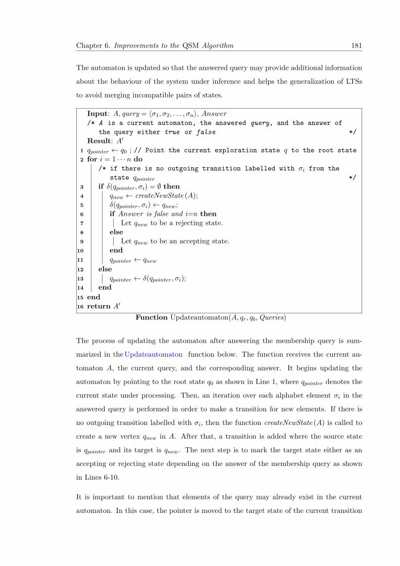
Chapter 6. Improvements to the QSM Algorithm 181
The automaton is updated so that the answered query may provide additional information
about the behaviour of the system under inference and helps the generalization of LTSs
to avoid merging incompatible pairs of states.
Input: A, query = 〈σ1, σ2, . . . , σn〉, Answer/* A is a current automaton, the answered query, and the answer of
the query either true or false */
Result: A′
1 qpointer ← q0 ; // Point the current exploration state q to the root state
2 for i = 1 · · ·n do/* if there is no outgoing transition labelled with σi from the
state qpointer */
3 if δ(qpointer, σi) = ∅ then4 qnew ← createNewState (A);5 δ(qpointer, σi)← qnew;6 if Answer is false and i=n then7 Let qnew to be a rejecting state.8 else9 Let qnew to be an accepting state.
10 end11 qpointer ← qnew12 else13 qpointer ← δ(qpointer, σi);14 end
15 end16 return A′
Function Updateautomaton(A, qr, qb,Queries)
The process of updating the automaton after answering the membership query is sum-
marized in the Updateautomaton function below. The function receives the current au-
tomaton A, the current query, and the corresponding answer. It begins updating the
automaton by pointing to the root state q0 as shown in Line 1, where qpointer denotes the
current state under processing. Then, an iteration over each alphabet element σi in the
answered query is performed in order to make a transition for new elements. If there is
no outgoing transition labelled with σi, then the function createNewState (A) is called to
create a new vertex qnew in A. After that, a transition is added where the source state
is qpointer and its target is qnew. The next step is to mark the target state either as an
accepting or rejecting state depending on the answer of the membership query as shown
in Lines 6-10.
It is important to mention that elements of the query may already exist in the current
automaton. In this case, the pointer is moved to the target state of the current transition
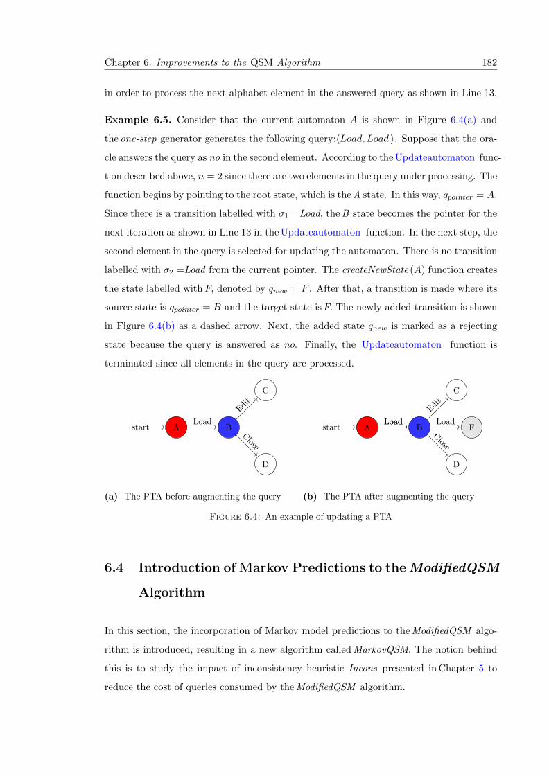
Chapter 6. Improvements to the QSM Algorithm 182
in order to process the next alphabet element in the answered query as shown in Line 13.
Example 6.5. Consider that the current automaton A is shown in Figure 6.4(a) and
the one-step generator generates the following query:〈Load, Load 〉. Suppose that the ora-
cle answers the query as no in the second element. According to the Updateautomaton func-
tion described above, n = 2 since there are two elements in the query under processing. The
function begins by pointing to the root state, which is the A state. In this way, qpointer = A.
Since there is a transition labelled with σ1 =Load, the B state becomes the pointer for the
next iteration as shown in Line 13 in the Updateautomaton function. In the next step, the
second element in the query is selected for updating the automaton. There is no transition
labelled with σ2 =Load from the current pointer. The createNewState (A) function creates
the state labelled with F, denoted by qnew = F . After that, a transition is made where its
source state is qpointer = B and the target state is F. The newly added transition is shown
in Figure 6.4(b) as a dashed arrow. Next, the added state qnew is marked as a rejecting
state because the query is answered as no. Finally, the Updateautomaton function is
terminated since all elements in the query are processed.
Astart B
C
D
Load
Edit
Close
(a) The PTA before augmenting the query
Astart B
C
D
FLoadLoad
Edit
Load
Close
(b) The PTA after augmenting the query
Figure 6.4: An example of updating a PTA
6.4 Introduction of Markov Predictions to the ModifiedQSM
Algorithm
In this section, the incorporation of Markov model predictions to the ModifiedQSM algo-
rithm is introduced, resulting in a new algorithm called MarkovQSM. The notion behind
this is to study the impact of inconsistency heuristic Incons presented in Chapter 5 to
reduce the cost of queries consumed by the ModifiedQSM algorithm.

Chapter 6. Improvements to the QSM Algorithm 183
In general, MarkovQSM constructs the initial Markov model from the collected abstracted
traces as described in Chapter 5. For each pair of states, the Incons is computed based on
the current Markov model. The pair of states are considered for merging without asking
membership queries whenever the EDSM score is higher than or equal to the Incons score.
In this case no queries are generated since there is evidence suggesting the pair of states
are equivalent. MarkovQSM is an active learner of LTS models in which it obtains new
information during the inference process after asking membership queries. Hence, the
Markov model should be updated since additional analysis of the system under inference
is obtained.
The following subsections discuss the usage of the Markov model with the Markov QSM
algorithm in detail. Section 6.4.1 discusses the strategy of updating the Markov model after
answering membership queries. Finally, Section 6.4.2 presents the Markov QSM algorithm
that is designed to reduce the number of membership queries that are answered by an
oracle.
6.4.1 Updating the Markov Matrix
This section introduces a method of updating the Markov matrix (MT) after answer-
ing membership queries. During the inference process, using the MarkovQSM algorithm,
which will be described later in this chapter, the trained MT that is built based on the
initial traces should be updated since membership queries that are asked may exercise a
new aspect of a system under inference.
The idea of updating the MT begins by given a membership query σ1, σ2, . . . , σn that
is answered by an oracle, and the value of prefix length k that is used to construct the
initial Markov model. Then, it calls the automatic Markov updater (MU) that looks at
subsequences of length k + 1 in the membership query to update the Markov matrix as
follows:
� If the membership query is answered as yes denoting that the query belongs to the
language of LTS, the MU records a pair (〈σi, σi+1, . . . , σi+k−1〉, σi+k) as a positive if
it is seen for the first time. We write ML : (〈σi, σi+1, . . . , σi+k−1〉, σi+k) 7→ Pos to

Chapter 6. Improvements to the QSM Algorithm 184
denote that σi+k is predicted by the Markov prediction function ML as a permitted
element of alphabet to follow the sequence 〈σi, σi+1, . . . , σi+k−1〉.
� The pair (〈σi, σi+1, . . . , σi+k−1〉, σi+k) is recorded as negative if it is never seen by
the Markov model and observed at the end of a membership query that is answered
as no. In this case, i+ k = n. We write ML : (〈σi, σi+1, . . . , σi+k−1〉, σi+k) 7→ Neg to
denote that σi+k is predicted by the Markov prediction function ML as not permitted
to follow the prefix sequence of length k 〈σi, σi+1, . . . , σi+k−1〉.
� The pair (〈σi, σi+1, . . . , σi+k−1〉, σi+k) is updated to failure if it is already observed
in the Markov model as a positive and it is at the end of a membership query that
is answered as no such that i+ k = n. On the other hand, if the oracle answers
the membership query as yes where (〈σi, σi+1, . . . , σi+k−1〉, σi+k) is already observed
in the Markov model as a negative subsequence, it is updated to failure. In this
case, we write ML : (〈σi, σi+1, . . . , σi+k−1〉, σi+k) 7→ Fail to denote that σi+k is not
predicted by the Markov prediction function ML during the computation of the in-
consistency score. This differs from the non-observed subsequence, and we write ML :
(〈σi, σi+1, . . . , σi+k−1〉, σi+k) /∈ dom(MT) to denote that (〈σi, σi+1, . . . , σi+k−1〉, σi+k)
has not been seen so far.
The algorithm of updating the Markov model is called UpdateMarkov and is shown below
in Algorithm 13. It starts by providing the current Markov table MT , the query, and its
answer. The provided query is a sequence of alphabet elements. If the query is answered
as no, it is passed to the algorithm up to the element of alphabet that caused the oracle
to reject the query. For example, if a given query σ1, σ2, σ3, . . . , σn is answered as no at
the element σ2, then σ1, σ2 is passed to the UpdateMarkov algorithm. On the other hand,
all alphabet elements of the query that are answered as yes are passed to the algorithm.
Algorithm 13 then obtains subsequences of length k + 1 iteratively from the provided
query. The obtainSubsequence (query, i, k) function is responsible for obtaining the current
subsequence from σi to σk+i of length k+ 1. If the obtained subsequence does not belong
to the MT, denoted by (〈σi, σi+1, . . . , σi+k−1〉, σi+k) /∈ dom(MT), then the procedure in
Lines 4-8 is performed to record the newly observed subsequences. On the other hand, if
the subsequence belongs to the MT, the updating procedure of the MT is shown in Lines
10-16.

Chapter 6. Improvements to the QSM Algorithm 185
Input: MT, query = 〈σ1, σ2, . . . , σn〉, Answer/* MT is the Markov table, the answered query, and the answer of the
query either true or false */
// The result is the updated Markov table
Result: MT ′
// Declare the prefix length KDeclare: K ← Integer
1 for i = 1 · · ·n do2 〈σi, σi+1, . . . , σi+k−1, σi+k〉 ← obtainSubsequence (query, i,K);
/* if the subsequence 〈σi, σi+1, . . . , σi+k−1, σi+k〉 is seen for the first
time */
3 if (〈σi, σi+1, . . . , σi+k−1〉, σi+k) /∈ dom (MT ) then4 if Answer is false and i+ k = n then5 Record a pair (〈σi, σi+1, . . . , σi+k−1〉, σi+k) in MT as a negative
subsequence.6 MT ′ = MT ⊕ {(〈σi, σi+1, . . . , σi+k−1〉, σi+k) 7→ Neg}7 else8 Record a pair (〈σi, σi+1, . . . , σi+k−1〉, σi+k) in MT as a positive
subsequence.9 MT ′ = MT ⊕ {(〈σi, σi+1, . . . , σi+k−1〉, σi+k) 7→ Pos}
10 end
11 else/* Otherwise the subsequnce 〈σi, σi+1, . . . , σi+k−1, σi+k〉 is already
seen in MT */
12 if Answer is false and i+ k = n and(〈σi, σi+1, . . . , σi+k−1〉, σi+k) 7→ true ∈ ML then
13 Update a pair (〈σi, σi+1, . . . , σi+k−1〉, σi+k) in MT to be a failuresubsequence.
14 MT ′ = MT ⊕ {(〈σi, σi+1, . . . , σi+k−1〉, σi+k) 7→ Fail}15 else16 if Answer is yes and (〈σi, σi+1, . . . , σi+k−1〉, σi+k) 7→ false ∈ ML then17 Update a pair (〈σi, σi+1, . . . , σi+k−1〉, σi+k) in MT to be a failure
subsequence.18 MT ′ = MT ⊕ {(〈σi, σi+1, . . . , σi+k−1〉, σi+k) 7→ Fail}19 end
20 end
21 end
22 end23 return MT
Algorithm 13: The UpdateMarkov algorithm
Example 6.6. Suppose that the current automaton during the induction process is shown
in Figure 6.5, and consider that the corresponding MT is shown in Table 6.1a where
k = 1. Let us consider the D state is chosen to merge with the B state. Assume that the
oracle answers the following membership query: 〈Load, Load〉, which is generated using

Chapter 6. Improvements to the QSM Algorithm 186
the Dupont generator, as no. In this example, there is one subsequence: {〈Load, Load〉}
of length k + 1 observed in the membership query. Following the above description of
updating the MT , the subsequence {〈Load, Load〉} is considered as a new subsequence
for the MT that is shown in Table 6.1a. The Markov model is then updated by recording
{〈Load, Load〉} as negative, as shown in Table 6.1b.
Astart B
C
D
G
E
H I
KLoad
Edit
Close
Edit
Save
Save Close
Load
Figure 6.5: The automaton before asking queries
Astart B
C
G
E
H I
KLoad
Edit
Close
Load
Edit
Save
Save Close
Figure 6.6: The automaton after merging B and D
Load Edit Save Close
Load - Pos - PosEdit - Pos Pos -Save - - - PosClose Pos - - -
(a) The Markov matrix before asking querieswhere k = 1
Load Edit Save Close
Load Neg Pos - PosEdit - Pos Pos -Save - - - PosClose Pos - - -
(b) The Markov matrix after asking querieswhere k = 1
Table 6.1: An example of updating the Markov table when k = 1
Example 6.7. Figure 6.7 shows the current automaton during the inference process.
Table 6.2a illustrates the corresponding MT where k = 2. Let us consider the pair of states
(G,C) is considered to compute its score. Assume that the oracle answers the following
membership query: 〈Load,Edit, Edit, Edit〉, which is generated using the one-step genera-
tor, as yes. In this example, there are two subsequences: {〈Load,Edit, Edit〉, 〈Edit, Edit, Edit〉}
of length k+ 1 observed in the membership query. Following the above description of up-
dating the Markov model, the subsequence {〈Load,Edit, Edit〉} is already seen in the MT ,

Chapter 6. Improvements to the QSM Algorithm 187
and the subsequence {〈Edit, Edit, Edit〉} is considered as a new subsequence for the MT
that is shown in Table 6.2a. The MT is then updated by recording {〈Edit, Edit, Edit〉}
as positive, as shown in Table 6.2b.
Astart B
C
D K
G
E
H I
F H J L
Load
Edit
Close
Edit
Save
Save Close
Edit Save Edit Save
Load
Figure 6.7: The automaton before asking queries
Load Edit Save Close
Load, Load - - - -Load, Edit - Pos Pos -Load, Save - - - -Load, Close Pos - - -Edit, Load - - - -Edit, Edit - - Pos -Edit, Save - - - PosEdit, Close - - - -Save, Load - - - -Save, Edit - - - -Save, Save - - - -Save, Close - - - -Close, Load - - - -Close, Edit - - - -Close, Save - - - -Close, Close - - - -
(a) The Markov matrix before asking querieswhere k = 2
Load Edit Save Close
Load, Load - - - -Load, Edit - Pos Pos -Load, Save - - - -Load, Close Pos - - -Edit, Load - - - -Edit, Edit - Pos Pos -Edit, Save - - - PosEdit, Close - - - -Save, Load - - - -Save, Edit - - - -Save, Save - - - -Save, Close - - - -Close, Load - - - -Close, Edit - - - -Close, Save - - - -Close, Close - - - -
(b) The Markov matrix after asking querieswhere k = 2
Table 6.2: An example of updating the Markov table when k = 2

Chapter 6. Improvements to the QSM Algorithm 188
6.4.2 The ModifiedQSM With Markov Predictions
This section presents the MarkovQSM algorithm, which is an extension to the ModifiedQSM
algorithm. The objective of the MarkovQSM algorithm is to study the influence of com-
putation of inconsistency on the accuracy of the inferred models and on the number
of membership queries that are consumed using the ModifiedQSM algorithm. Hence,
the MarkovQSM algorithm incorporates Markov predictions and the computation of the
inconsistency during the evaluation of each pair of states for merging.
The induction process of an LTS using the MarkovQSM is summarized in Algorithm 14.
Similar to the ModifiedQSM learner, MarkovQSM begins by constructing the initial PTA
from the positive traces. The Markov matrix is trained from the same traces as shown
in line 2. The Markov matrix is built in the same way that is used in the EDSM-Markov
algorithm, which is described in Chapter 5. The process continues in the same way as
in ModifiedQSM except that membership queries are only generated if the inconsistency
score Im =(Incons(merge(A, q, q′),ML)−Incons(A,ML)
)is greater than the EDSM score
as shown in Line 15, as shown in Algorithm 14. The idea behind asking queries in this
case is to measure and determine whether the pair of states are equivalent or not.
It is important to highlight that a pair of states are added to the PossiblePairs set if
the EDSM score is higher than or equal to the inconsistency score (see Lines 24-25); this
denotes that there is evidence suggesting that states in the pair are equivalent and it is
not necessary to ask membership queries in this stage.
The strategy of processing membership queries in the MarkovQSM is performed in the
same way in ModifiedQSM, except that the Markov model is updated after answering
each membership query as described in Section 6.4.1. The step of updating the Markov
table is performed using the updateMarkovTable (MT, query,Answer) function in Line 4,
as illustrated in the processQuerieswithMarkov function. The inference of LTS models
using the MarkovQSM is terminated if all states in the current automaton are coloured
red.

Chapter 6. Improvements to the QSM Algorithm 189
6.5 Conclusion
This chapter introduced the ModifiedQSM state-merging inference algorithm that improves
the accuracy of the inferred models in comparison with QSM. The one-step generator is
introduced to help the proposed learners to avoid the over-generalization issue.
An alternative extension of the ModifiedQSM learner has been introduced, known as
MarkovQSM. It relies upon training Markov models from the provided traces and up-
dating Markov models after asking each query. It allows the MarkovQSM learner posing
membership queries only if an inconsistency score Im is greater than an EDSM score.

Chapter 6. Improvements to the QSM Algorithm 190
input : S+, S−
/* Sets of accepted S+ and rejected S− sequences */
result: A is an LTS that is compatible with S+, S−, and generated queries
1 A← generatePTA (S+, S−);2 MT← trainMarkovTable (S+, S−);3 R← {q0} ; // R is a set of red states
4 do5 do6 PossiblePairs← ∅ ; // PossiblePairs possible pairs to merge
7 Rextended← false ;8 B ← ComputeBlue(A,R) ; // B is a set of blue states
9 for qb ∈ B do10 mergeable← false ;11 compatible← false ;12 for qr ∈ R do13 compatible← checkMergeCompatibility (A, qr, qb);14 if compatible then15 if Im is greater than EDSM score then16 Queries← generateDupontQueries (A, qr, qb);17 Queries← Queries ∪ generateOneStepQuery (A, qr, qb);
/* update automaton A′ after asking queries */
18 A← processQueries (A, qr, qb,Queries);19 if EDSMScore (A, qr, qb) >= 0 then20 PossiblePairs← PossiblePairs ∪ {(qr, qb)} ;21 mergeable← true ;
22 end
23 else24 PossiblePairs← PossiblePairs ∪ {(qr, qb)} ;25 mergeable← true ;
26 end
27 end
28 end29 if mergeable = false then30 R← R ∪ {qb};31 Rextended← true ;
32 end
33 end
34 while Rextended = true;35 if PossiblePairs 6= ∅ then36 (qr, qb)← PickPair (PossiblePairs);37 if EDSMScore (A, qr, qb) >= 0 then38 A← merge (A, qr, qb);39 end
40 end
41 while PossiblePairs 6= ∅;42 return A
Algorithm 14: The Markov QSM algorithm

Chapter 6. Improvements to the QSM Algorithm 191
Input: A, qr, qb,Queries,MT/* A is a current PTA hypothesis, Queries */
Result: The updated PTA A′
1 while query ← Queries do2 Answer ← checkWithOracle (query);
3 A′ ← updateAutomaton (A,Answer);
4 MT← updateMarkovTable (MT, query,Answer);5 score← ComputeEDSMScore (A′, qr, qb);6 if score < 0 then
/* Terminate */
7 Break
8 end
9 end10 return A′
Function processQuerieswithMarkov(A, qr, qb,Queries,MT )
7Experimental Evaluation of ModifiedQSM and
MarkovQSM
7.1 Introduction
In the previous chapter, the ModifiedQSM and MarkovQSM learners were introduced.
The main purpose of establishing them is to infer LTS models from a few traces. This
chapter evaluates the performance of the proposed learners using both randomly generated
LTSs and case studies.
The following section presents the experimental evaluation of the proposed algorithms.
The aim of running experiments is to assess the capability of the ModifiedQSM and
MarkovQSM learners at improving the accuracy of the inferred models.
192

Chapter 7. Experimental Evaluation of ModifiedQSM and MarkovQSM 193
7.2 Experimental Setup and Evaluation
This section presents the investigation and studies the performance of the ModifiedQSM
and MarkovQSM learners. It includes a comparison of the developed algorithms compared
to QSM. The measurements were performed based on different criteria. The experiment
aimed to address and investigate the following research questions:
1. Do the ModifiedQSM and MarkovQSM infer LTS models better than QSM ?
2. What is the impact of introducing the inconsistency computation in MarkovQSM
on the accuracy of the inferred models and on the number of membership queries
compared to other algorithms?
In order to evaluate the performance of the ModifiedQSM and MarkovQSM, a series of
random LTSs were generated in different sizes (number of states): 10, 20 and 30. The
randomly-generated LTSs were connected and had different alphabet sizes to vary their
complexity. In this way, an alphabet multiplier parameter m was introduced to vary the
alphabet size so that |Σ| = m ∗ |Q|, where m was set to 0.5, 1, and 2 in this experiment.
Furthermore, the performance of ModifiedQSM and MarkovQSM were evaluated with
different numbers of traces T : 3 and 5 that were obtained by a random walk of the
generated LTSs. The length of the traces is |Q| ∗ |Σ| (= 0.125 ∗ |Q|2 ∗ 2). This length was
chosen since the passive inference in the previous chapter failed to learn good LTSs in this
setting. So, it is interesting to select this length of traces to compare between different
learners. The mean value of the BCR scores in the passive experiment was around 0.55
where the number of traces is 5. Hence, it is better to study the improvement made by
the concept of active learning with the worst case in the passive experiment in Chapter 6.
Specifically, ten LTSs were randomly generated for each chosen size of state and each
alphabet multiplier. Thus, 10-30 states is 3 steps ∗ 10 LTSs = 30 LTSs in total for each
m setting. For each LTS, three sets of training data were generated, bringing the number
of LTSs learnt per experiment to 90 for each setting of T , under an assumption that the
same training data is passed for the learners for each evaluation task. The idea behind
learning this number of LTSs is to assess the performance of the proposed algorithms on
various numbers of random LTSs with different training data fed to each LTS.
Chapter 7. Experimental Evaluation of ModifiedQSM and MarkovQSM 194
In the original study of QSM by Dupont et al. [36], the evaluation of the QSM is made
using random LTSs where the alphabet size was two; both positive and negative samples
were supplied to the learner. Walkinshaw et al. [28] evaluated the efficiency of their QSM
using random LTS where the alphabet size is six, and only positive traces were provided to
start the inference process. In this experiment, ModifiedQSM and MarkovQSM learners
will be evaluated against Dupont’s QSM where the size of alphabet is large, and only a
few positive traces are provided.
In this experiment, BCR and structural-similarity metrics were selected to score the per-
formance of the algorithms. In addition, the number of membership queries was chosen
to measure the efficiency of the algorithms.
The implementation of this experiment is available for clone via https://github.com/
AbdullahUK/EDSM_QSM_MarkovPhd.git. For the conducted experiment, the launch con-
figuration has to start statechum.analysis.learning.experiments.PairSelection.
MarkovActiveExperiment class.
In the conducted experiments, Java 7 was used with JVM arguments of -ea -Dthreadnum=1
-Djava.library.path=linear/.libs;"C:/Program Files/R/R-3.0.1/library/rJava
/jri/x64" -Xmx26000m and environment variable R HOME set to the location of R, such as
C:/Program Files/R/R-3.0.1/lib64/R java. The R toolset was used for all analysis.
The R tool has to have JavaGD, rJava and aplpack installed.
7.2.1 Evaluating the Performance of ModifiedQSM and MarkovQSM
in Terms of BCR Scores
The boxplots of the BCR values produced by MarkovQSM, ModifiedQSM, and QSM are de-
picted in Figure 7.1. It is clear that the BCR scores of LTSs inferred using the ModifiedQSM
learner are the highest compared to both MarkovQSM and ModifiedQSM. It can be seen
from Figure 7.1 that MarkovQSM, at every number of traces, inferred LTSs with higher
BCR score compared to QSM.
Table 7.1 summarizes the median values of the BCR scores of LTSs inferred achieved
by MarkovQSM, ModifiedQSM and QSM. In addition, there is an obvious reduction in the

Chapter 7. Experimental Evaluation of ModifiedQSM and MarkovQSM 195
3 5
0.4
0.5
0.6
0.7
0.8
0.9
1.0
m=0.5 m=1.0 m=2.0 m=0.5 m=1.0 m=2.0alphabet Muliplier
BC
R s
core
s
MarkovQSM ModifiedQSM QSM
Trace Number
Figure 7.1: Boxplots of BCR scores achieved by various learners for different settingof m and T
Median
m Trace Number T ModifiedQSM MarkovQSM QSM
0.53 0.95 0.91 0.795 0.98 0.95 0.87
1.03 0.89 0.88 0.785 0.96 0.95 0.87
2.03 0.85 0.85 0.775 0.94 0.95 0.89
Table 7.1: The median values of BCR scores obtained by ModifiedQSM, MarkovQSM,and QSM
BCR scores attained by MarkovQSM compared to ModifiedQSM when m = 0.5. Addi-
tionally, the average BCR scores of LTSs inferred using MarkovQSM decreased by 6.52%
compared to the scores attained by ModifiedQSM when the number of traces is 3 and when
m = 0.5.
In order to statistically measure the significant difference between the resulting BCR scores
of LTSs obtained using the proposed algorithms against QSM, the paired Wilcoxon signed-
rank test was conducted between the BCR scores of the three algorithms at the signifi-
cance level of 0.05 (α = 0.05). Table 7.2 summarizes the statistical test results using the
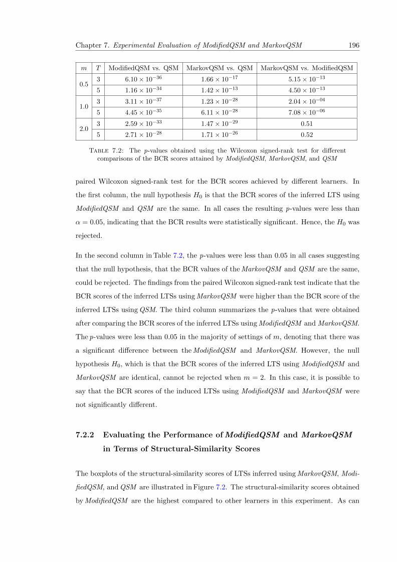
Chapter 7. Experimental Evaluation of ModifiedQSM and MarkovQSM 196
m T ModifiedQSM vs. QSM MarkovQSM vs. QSM MarkovQSM vs. ModifiedQSM
0.53 6.10× 10−36 1.66× 10⁻¹⁷ 5.15× 10⁻¹³
5 1.16× 10⁻³⁴ 1.42× 10⁻¹³ 4.50× 10⁻¹³
1.03 3.11× 10−37 1.23× 10⁻²⁸ 2.04× 10−04
5 4.45× 10⁻³⁵ 6.11× 10⁻²⁸ 7.08× 10−06
2.03 2.59× 10⁻³³ 1.47× 10⁻²⁹ 0.51
5 2.71× 10⁻²⁸ 1.71× 10⁻²⁶ 0.52
Table 7.2: The p-values obtained using the Wilcoxon signed-rank test for differentcomparisons of the BCR scores attained by ModifiedQSM, MarkovQSM, and QSM
paired Wilcoxon signed-rank test for the BCR scores achieved by different learners. In
the first column, the null hypothesis H0 is that the BCR scores of the inferred LTS using
ModifiedQSM and QSM are the same. In all cases the resulting p-values were less than
α = 0.05, indicating that the BCR results were statistically significant. Hence, the H0 was
rejected.
In the second column in Table 7.2, the p-values were less than 0.05 in all cases suggesting
that the null hypothesis, that the BCR values of the MarkovQSM and QSM are the same,
could be rejected. The findings from the paired Wilcoxon signed-rank test indicate that the
BCR scores of the inferred LTSs using MarkovQSM were higher than the BCR score of the
inferred LTSs using QSM. The third column summarizes the p-values that were obtained
after comparing the BCR scores of the inferred LTSs using ModifiedQSM and MarkovQSM.
The p-values were less than 0.05 in the majority of settings of m, denoting that there was
a significant difference between the ModifiedQSM and MarkovQSM. However, the null
hypothesis H0, which is that the BCR scores of the inferred LTS using ModifiedQSM and
MarkovQSM are identical, cannot be rejected when m = 2. In this case, it is possible to
say that the BCR scores of the induced LTSs using ModifiedQSM and MarkovQSM were
not significantly different.
7.2.2 Evaluating the Performance of ModifiedQSM and MarkovQSM
in Terms of Structural-Similarity Scores
The boxplots of the structural-similarity scores of LTSs inferred using MarkovQSM, Modi-
fiedQSM, and QSM are illustrated in Figure 7.2. The structural-similarity scores obtained
by ModifiedQSM are the highest compared to other learners in this experiment. As can

Chapter 7. Experimental Evaluation of ModifiedQSM and MarkovQSM 197
be seen in Figure 7.2, MarkovQSM inferred LTSs with poor structural-similarity scores in
many cases, especially when m = 0.5. This is due to earlier incorrect mergers that are
allowed which should do not happened (over-generalization). This denotes queries should
be asked in those cases. The median values of the structural-similarity scores of the learnt
LTSs using MarkovQSM, ModifiedQSM and QSM are summarized in Table 7.3.
3 5
0.2
0.3
0.4
0.5
0.6
0.7
0.8
0.9
1.0
m=0.5 m=1.0 m=2.0 m=0.5 m=1.0 m=2.0alphabet Muliplier
stru
ctur
al−
sim
ilarit
y S
core
s
MarkovQSM ModifiedQSM QSM
Trace Number
Figure 7.2: Boxplots of structural-similarity scores attained by ModifiedQSM,MarkovQSM, and QSM learners for different setting of m and T
Median
m T ModifiedQSM MarkovQSM QSM
0.53 0.97 0.92 0.855 0.99 0.96 0.90
1.03 0.96 0.95 0.875 0.98 0.98 0.92
2.03 0.95 0.94 0.905 0.98 0.97 0.94
Table 7.3: The median values of structural-similarity scores attained by ModifiedQSM,MarkovQSM, and QSM

Chapter 7. Experimental Evaluation of ModifiedQSM and MarkovQSM 198
The results, which are illustrated in Figure 7.2, show that the structural-similarity scores
of LTSs inferred using the MarkovQSM when m = 0.5 are worse than those inferred using
QSM in some cases. Hence, it was necessary to measure the significant difference between
the structural-similarity scores attained by different learners. This was measured using
the paired Wilcoxon signed-rank test for the structural-similarity scores achieved using
various algorithms. When comparing the structural-similarity scores of the inferred models
using QSM against ModifiedQSM, the null hypothesis H0, that the structural-similarity
scores between both algorithms are the same, was rejected. This was because the p-values
were less than 0.05 in all cases, as shown in the first column in Table 7.4.
m T ModifiedQSM vs. QSM MarkovQSM vs. QSM MarkovQSM vs. ModifiedQSM
0.53 3.26× 10−38 0.06 1.58× 10⁻²¹
5 9.81× 10⁻³⁵ 0.21 1.42× 10⁻²⁰
1.03 4.31× 10−37 1.50× 10⁻¹³ 1.61× 10⁻¹⁰
5 7.60× 10⁻³⁵ 1.31× 10⁻¹² 7.45× 10−08
2.03 4.91× 10⁻³⁴ 1.42× 10⁻¹⁸ 9.70× 10−04
5 2.95× 10⁻²⁹ 1.27× 10⁻¹⁷ 2.58× 10−05
Table 7.4: The p-values obtained using the Wilcoxon signed-rank test for differentcomparisons of the structural-similarity scores attained by ModifiedQSM, MarkovQSM,
and QSM
The second column in Table 7.4 summarizes the resulting p-values when comparing the
structural-similarity scores of the inferred LTSs using QSM and MarkovQSM. In this study,
the null hypothesis H0 states that there is no significant difference between the structural-
similarity scores of the inferred LTS model using MarkovQSM and QSM. The p-values were
less than 0.05 when m >= 1, indicating that MarkovQSM inferred LTSs with higher
structural-similarity scores compared to QSM in the majority of inferred LTSs. Hence,
the H0 can be rejected. However, the p-values were higher than 0.05 when m = 0.5, so
the H0 cannot be rejected.
Additionally, the third column in Table 7.4 reports the resulting p-values after comparing
the structural-similarity scores of the inferred LTSs using MarkovQSM and ModifiedQSM.
The null hypothesis H0 in this comparison states that there is no significant difference
between MarkovQSM and ModifiedQSM in terms of the structural-similarity scores. In
all cases, the p-values were less than 0.05, the null hypothesis could be rejected.

Chapter 7. Experimental Evaluation of ModifiedQSM and MarkovQSM 199
7.2.3 Number of Membership Queries
An important factor that must be taken into consideration while evaluating the perfor-
mance of ModifiedQSM, MarkovQSM, and QSM is the number of membership queries that
are submitted to the oracle. Figure 7.3 illustrates the number of membership queries
submitted to the oracle when m = 0.5. Interestingly, when the number of states was 30,
the average number of membership queries that were asked by MarkovQSM decreased by
1.43% compared to QSM, and reduced by 11.63% compared to ModifiedQSM.
10 20 30
0
50
100
150
200
0
250
500
750
1000
500
1000
1500
2000
2500
T=3 T=5 T=3 T=5 T=3 T=5Trace Number
num
ber
of m
embe
rshi
p qu
erie
s
MarkovQSM ModifiedQSM QSM
State Number
Figure 7.3: The number of membership queries that were asked by different learnerswhen m = 0.5
Table 7.5 shows the median values of the number of membership queries when m =
0.5. When the number of states was 30, the median value of the number of membership
queries that were asked by MarkovQSM were less than the median value of the consumed
membership queries using other algorithms. Otherwise, the smallest median value of the
number of membership queries was observed for the QSM algorithm.
The paired Wilcoxon signed-rank statistical test was used to statistically measure the
significant difference between the number of membership queries that were asked by dif-
ferent learners. The null hypothesis H0 states that there is no significant difference in
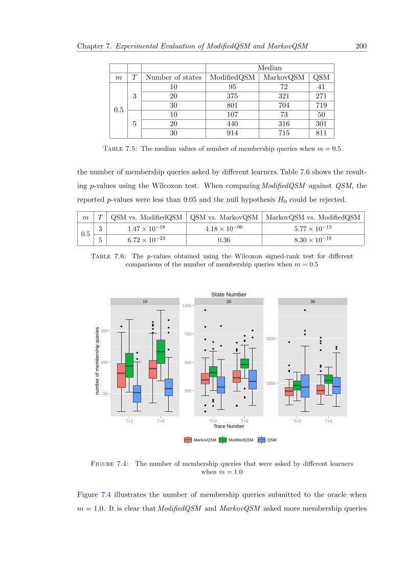
Chapter 7. Experimental Evaluation of ModifiedQSM and MarkovQSM 200
Median
m T Number of states ModifiedQSM MarkovQSM QSM
0.5
310 95 72 4120 375 321 27130 801 704 719
510 107 73 5020 440 316 30130 914 715 811
Table 7.5: The median values of number of membership queries when m = 0.5
the number of membership queries asked by different learners. Table 7.6 shows the result-
ing p-values using the Wilcoxon test. When comparing ModifiedQSM against QSM, the
reported p-values were less than 0.05 and the null hypothesis H0 could be rejected.
m T QSM vs. ModifiedQSM QSM vs. MarkovQSM MarkovQSM vs. ModifiedQSM
0.53 1.47× 10⁻¹⁸ 4.18× 10−06 5.77× 10⁻¹³
5 6.72× 10⁻²³ 0.36 8.30× 10⁻¹⁶
Table 7.6: The p-values obtained using the Wilcoxon signed-rank test for differentcomparisons of the number of membership queries when m = 0.5
10 20 30
50
100
150
250
500
750
1000
1000
2000
T=3 T=5 T=3 T=5 T=3 T=5Trace Number
num
ber
of m
embe
rshi
p qu
erie
s
MarkovQSM ModifiedQSM QSM
State Number
Figure 7.4: The number of membership queries that were asked by different learnerswhen m = 1.0
Figure 7.4 illustrates the number of membership queries submitted to the oracle when
m = 1.0. It is clear that ModifiedQSM and MarkovQSM asked more membership queries
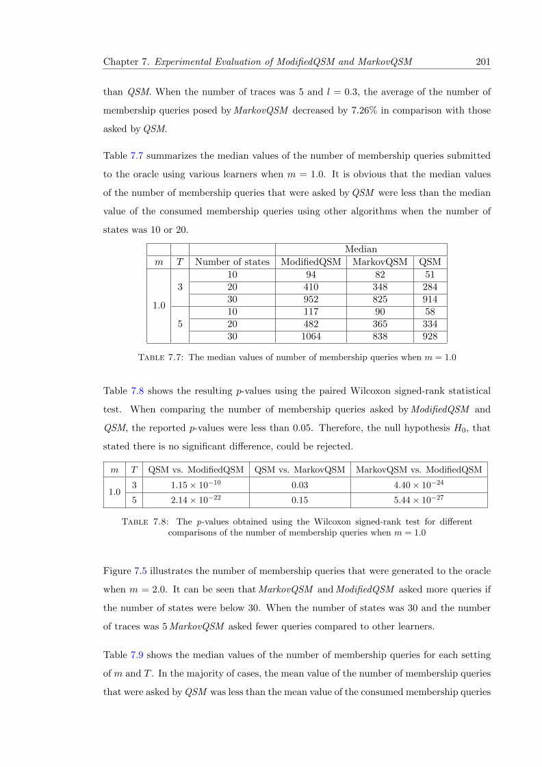
Chapter 7. Experimental Evaluation of ModifiedQSM and MarkovQSM 201
than QSM. When the number of traces was 5 and l = 0.3, the average of the number of
membership queries posed by MarkovQSM decreased by 7.26% in comparison with those
asked by QSM.
Table 7.7 summarizes the median values of the number of membership queries submitted
to the oracle using various learners when m = 1.0. It is obvious that the median values
of the number of membership queries that were asked by QSM were less than the median
value of the consumed membership queries using other algorithms when the number of
states was 10 or 20.
Median
m T Number of states ModifiedQSM MarkovQSM QSM
1.0
310 94 82 5120 410 348 28430 952 825 914
510 117 90 5820 482 365 33430 1064 838 928
Table 7.7: The median values of number of membership queries when m = 1.0
Table 7.8 shows the resulting p-values using the paired Wilcoxon signed-rank statistical
test. When comparing the number of membership queries asked by ModifiedQSM and
QSM, the reported p-values were less than 0.05. Therefore, the null hypothesis H0, that
stated there is no significant difference, could be rejected.
m T QSM vs. ModifiedQSM QSM vs. MarkovQSM MarkovQSM vs. ModifiedQSM
1.03 1.15× 10⁻¹⁰ 0.03 4.40× 10⁻²⁴
5 2.14× 10⁻²² 0.15 5.44× 10⁻²⁷
Table 7.8: The p-values obtained using the Wilcoxon signed-rank test for differentcomparisons of the number of membership queries when m = 1.0
Figure 7.5 illustrates the number of membership queries that were generated to the oracle
when m = 2.0. It can be seen that MarkovQSM and ModifiedQSM asked more queries if
the number of states were below 30. When the number of states was 30 and the number
of traces was 5 MarkovQSM asked fewer queries compared to other learners.
Table 7.9 shows the median values of the number of membership queries for each setting
of m and T . In the majority of cases, the mean value of the number of membership queries
that were asked by QSM was less than the mean value of the consumed membership queries
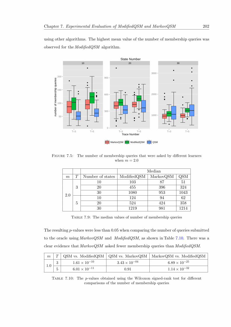
Chapter 7. Experimental Evaluation of ModifiedQSM and MarkovQSM 202
using other algorithms. The highest mean value of the number of membership queries was
observed for the ModifiedQSM algorithm.
10 20 30
50
100
150
200
0
300
600
900
1000
2000
3000
T=3 T=5 T=3 T=5 T=3 T=5Trace Number
num
ber
of m
embe
rshi
p qu
erie
s
MarkovQSM ModifiedQSM QSM
State Number
Figure 7.5: The number of membership queries that were asked by different learnerswhen m = 2.0
Median
m T Number of states ModifiedQSM MarkovQSM QSM
2.0
310 103 87 5120 455 396 32430 1080 953 1043
510 124 94 6220 524 424 35830 1219 981 1214
Table 7.9: The median values of number of membership queries
The resulting p-values were less than 0.05 when comparing the number of queries submitted
to the oracle using MarkovQSM and ModifiedQSM, as shown in Table 7.10. There was a
clear evidence that MarkovQSM asked fewer membership queries than ModifiedQSM.
m T QSM vs. ModifiedQSM QSM vs. MarkovQSM MarkovQSM vs. ModifiedQSM
1.03 1.61× 10⁻¹⁰ 3.43× 10−04 6.89× 10⁻²⁵
5 6.01× 10⁻¹¹ 0.91 1.14× 10⁻³²
Table 7.10: The p-values obtained using the Wilcoxon signed-rank test for differentcomparisons of the number of membership queries

Chapter 7. Experimental Evaluation of ModifiedQSM and MarkovQSM 203
Figure 7.6 illustrates the transition cover that was collected from the training data during
the conducted experiment. It is worth noting that the ModifiedQSM and MarkovQSM
generated better LTSs compared to the QSM even if many of those transitions in the
target LTSs were not covered. This is the advantage of considering one-step queries that
guide the learners to avoid merging states that are not equivalent in the target hidden
LTSs.
3 5
0
20
40
60
80
100
m=0.5 m=1.0 m=2.0 m=0.5 m=1.0 m=2.0Alphabet Muliplier
Tran
sitio
n C
over
age
%
Transitions coverage by traces
Trace Number
Figure 7.6: The transition cover of the generated traces
During the conducted experiments using random LTSs, it was interesting to compute the
Markov precision and recall scores of the trained Markov models. In this experiment, a low
precision was observed when m = 0.5 denoting that the trained Markov models predicted
transitions wrongly as shown in Figure 7.7. This may explains why the MarkovQSM did
perform well when m = 0.5 compared to other settings of m.
Besides, the performance of MarkovQSM are very close to ModifiedQSM when m = 2.0,
because both learners inferred LTSs with very similar BCR and structural-similarity scores.
This is due to the high precision value of the trained Markov model where m = 2.0. In
this case, inconsistencies were detected well whenever a merger added labels of outgoing
transitions that predicted incorrectly with respect to the trained Markov models.
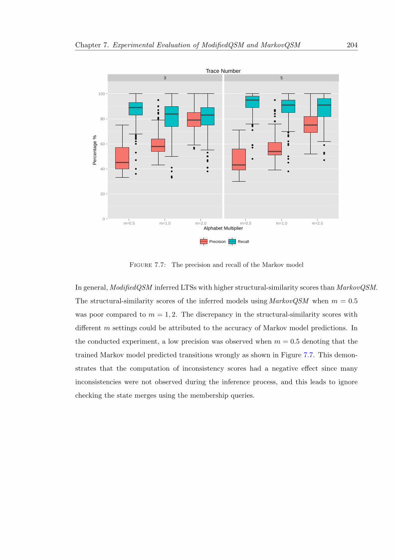
Chapter 7. Experimental Evaluation of ModifiedQSM and MarkovQSM 204
3 5
0
20
40
60
80
100
m=0.5 m=1.0 m=2.0 m=0.5 m=1.0 m=2.0Alphabet Multiplier
Per
cent
age
%
Precision Recall
Trace Number
Figure 7.7: The precision and recall of the Markov model
In general, ModifiedQSM inferred LTSs with higher structural-similarity scores than MarkovQSM.
The structural-similarity scores of the inferred models using MarkovQSM when m = 0.5
was poor compared to m = 1, 2. The discrepancy in the structural-similarity scores with
different m settings could be attributed to the accuracy of Markov model predictions. In
the conducted experiment, a low precision was observed when m = 0.5 denoting that the
trained Markov model predicted transitions wrongly as shown in Figure 7.7. This demon-
strates that the computation of inconsistency scores had a negative effect since many
inconsistencies were not observed during the inference process, and this leads to ignore
checking the state merges using the membership queries.

Chapter 7. Experimental Evaluation of ModifiedQSM and MarkovQSM 205
7.3 Case Studies
In the previous section, the efficiency of the ModifiedQSM and MarkovQSM learners
was evaluated on randomly-generated LTSs. It was clear that the ModifiedQSM learner
performed well compared to other learners. In this section, a number of case studies are
used to evaluate the efficiency of different learners to infer good LTSs. The performance
of the ModifiedQSM, MarkovQSM, and QSM learners was evaluated on a number of case
studies. For each of the following case studies, the number of traces ranged from two
to four, and the length of traces was given by l ∗ |Q| ∗ |Σ|, where l is a parameter to
control the length of generated traces. In the conducted experiment, 30 different random
traces were generated for each number and length of traces. In addition, 2× |Q| × |Q| test
sequences were generated of length 3 × |Q|. This was chosen to match the settings used
in the conducted experiments using random LTSs.
7.3.1 Case Study: SSH Protocol
2 3 4
0.4
0.5
0.6
0.7
0.8
0.9
1.0
L=0.1 L=0.3 L=0.1 L=0.3 L=0.1 L=0.3Trace Length Muliplier
BC
R s
core
MarkovQSM ModifiedQSM QSM
Trace Number
Figure 7.8: The BCR scores attained by ModifiedQSM, MarkovQSM, and QSM for theSSH protocol case study
The findings of the SSH case study are shown in Figure 7.8, and summarize the BCR
scores of the inferred models using different learners when l = 0.3 and 0.5 respectively.
From Figure 7.8, it is apparent that the inferred LTSs using ModifiedQSM and MarkovQSM

Chapter 7. Experimental Evaluation of ModifiedQSM and MarkovQSM 206
learners were close to the reference LTSs in terms of their language. It was noticed that
the QSM learner performed badly when l = 0.1 compared to other learners. This is
due to that Dupont’s QSM queries are insufficient to avoid merging incompatible pairs
of states, especially if few traces are provided. The improvement made by ModifiedQSM
and MarkovQSM learners over QSM was caused by the one-step queries and this made it
possible to detect incorrect states merges and avoid merging them.
Table 7.11 summarizes the p-values of BCR scores obtained from the Wilcoxon signed-
rank statistical test. The null hypothesis H0 states that the BCR scores of the inferred
LTS using the learners are the same. The resulting p-values suggest rejecting the H0
when comparing ModifiedQSM and MarkovQSM against QSM since the p-values are less
than 0.05 (significance level), and this indicates that there is a statistically significant
difference between them. In other words, there is strong evidence to support the alternative
hypothesis which stated the BCR scores of the inferred LTSs using ModifiedQSM and QSM
are not same. Besides, the H0 is accepted if the trace number is 4 and l = 0.3, which means
that there is no statistically significant difference between the three learners. However,
when comparing ModifiedQSM and MarkovQSM, the H0 is accepted.
lTrace Number
2 3 4
0.1
ModifiedQSM vs. QSM 1.77× 10−06 3.91× 10−06 1.76× 10−05
MarkovQSM vs. QSM 2.61× 10−06 3.91× 10−06 1.76× 10−05
ModifiedQSM vs. MarkovQSM 1 − −
0.3
ModifiedQSM vs. QSM 2.53× 10−04 0.004 0.08
MarkovQSM vs. QSM 2.53× 10−04 0.004 0.08
ModifiedQSM vs. MarkovQSM − − −
Table 7.11: p-values obtained using the Wilcoxon signed-rank test after comparing theBCR scores attained by ModifiedQSM, MarkovQSM, and QSM for the SSH protocol case
study
The performance of the ModifiedQSM learner was evaluated in Section 7.2 using randomly-
generated LTSs and was shown to significantly improve the structural-similarity scores of
the inferred LTSs compared to MarkovQSM and QSM learners. In this case study, the
structural-similarity scores of the inferred LTSs using both ModifiedQSM and MarkovQSM
were higher than QSM as illustrated in Figure 7.9. The average scores attained by ModifiedQSM
increased by 23.75% compared to the scores attained by QSM when l = 0.1 and the number
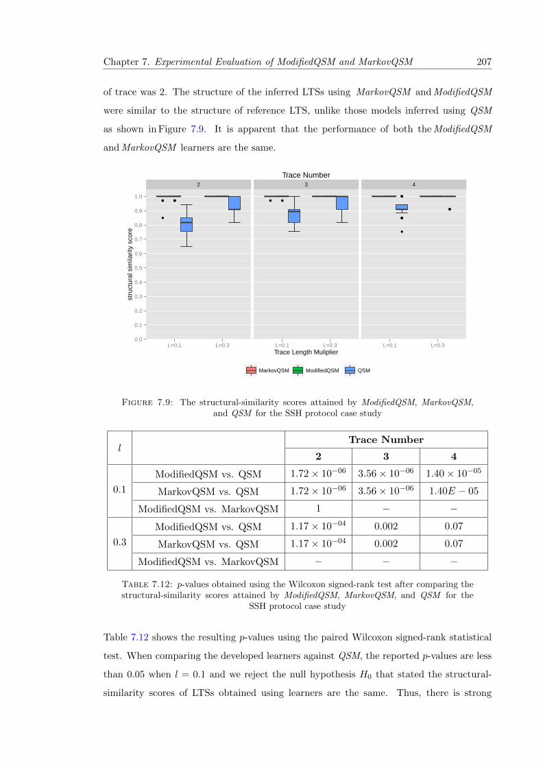
Chapter 7. Experimental Evaluation of ModifiedQSM and MarkovQSM 207
of trace was 2. The structure of the inferred LTSs using MarkovQSM and ModifiedQSM
were similar to the structure of reference LTS, unlike those models inferred using QSM
as shown in Figure 7.9. It is apparent that the performance of both the ModifiedQSM
and MarkovQSM learners are the same.
2 3 4
0.0
0.1
0.2
0.3
0.4
0.5
0.6
0.7
0.8
0.9
1.0
L=0.1 L=0.3 L=0.1 L=0.3 L=0.1 L=0.3Trace Length Muliplier
stru
ctur
al s
imila
rity
scor
e
MarkovQSM ModifiedQSM QSM
Trace Number
Figure 7.9: The structural-similarity scores attained by ModifiedQSM, MarkovQSM,and QSM for the SSH protocol case study
lTrace Number
2 3 4
0.1
ModifiedQSM vs. QSM 1.72× 10−06 3.56× 10−06 1.40× 10−05
MarkovQSM vs. QSM 1.72× 10−06 3.56× 10−06 1.40E − 05
ModifiedQSM vs. MarkovQSM 1 − −
0.3
ModifiedQSM vs. QSM 1.17× 10−04 0.002 0.07
MarkovQSM vs. QSM 1.17× 10−04 0.002 0.07
ModifiedQSM vs. MarkovQSM − − −
Table 7.12: p-values obtained using the Wilcoxon signed-rank test after comparing thestructural-similarity scores attained by ModifiedQSM, MarkovQSM, and QSM for the
SSH protocol case study
Table 7.12 shows the resulting p-values using the paired Wilcoxon signed-rank statistical
test. When comparing the developed learners against QSM, the reported p-values are less
than 0.05 when l = 0.1 and we reject the null hypothesis H0 that stated the structural-
similarity scores of LTSs obtained using learners are the same. Thus, there is strong

Chapter 7. Experimental Evaluation of ModifiedQSM and MarkovQSM 208
evidence to claim that ModifiedQSM and MarkovQSM outperformed QSM for the SSH
protocol case study. In addition, the H0 can be accepted in case where the number of
traces is 4 and l = 0.3. Furthermore, in case of comparing the structural-similarity scores
of the inferred LTSs using ModifiedQSM and MarkovQSM, the H0 is accepted since both
learners generated LTSs with similar structural-similarity scores.
Figure 7.10 shows the number of membership queries posed to the Oracle using various
algorithms. It shows that ModifiedQSM and MarkovQSM learners asked more queries
than QSM. This is due to the fact that ModifiedQSM and MarkovQSM learners posed the
one-step queries, unlike QSM that only asked Dupont’s queries; however, both learners im-
proved the BCR and structural-similarity scores of the inferred models. Numbers of mem-
bership queries that are posed using MarkovQSM was 1.96%slightly less than those posed
using ModifiedQSM when l = 0.1 and the number of traces is two. In addition, numbers
of membership queries were decreased by 5.45% when L = 0.3. Furthermore, MarkovQSM
asked fewer membership queries compared to ModifiedQSM when L = 0.3, due to the way
that queries are only asked if the Im score is higher than the EDSM score.
T=2 T=3 T=4
40
60
80
100
120
40
60
80
100
120
60
80
100
120
L=0.1 L=0.3 L=0.1 L=0.3 L=0.1 L=0.3Trace Number
num
ber
of m
embe
rshi
p qu
erie
s
MarkovQSM ModifiedQSM QSM
Tracenumber
Figure 7.10: The number of membership queries of different learners
To compare the number of membership queries that are posed using various learners, the
paired Wilcoxon signed-rank statistical test was used. Table 7.13 summarizes the resulting
p-values using the paired Wilcoxon signed-rank statistical test. The null hypothesis H0
Chapter 7. Experimental Evaluation of ModifiedQSM and MarkovQSM 209
states that the number of membership queries posed using the learners are the same. In
case of comparing the proposed learners against QSM, the reported p-values are less than
0.05 when l = 0.1. Thus, the null hypothesis H0 can be rejected, denoting that there is
strong evidence to say that QSM asked fewer queries than ModifiedQSM and MarkovQSM.
However, the H0 can be accepted in case of comparing MarkovQSM and QSM if the
number of traces is four and l = 0.3. When comparing the number of membership queries
that were asked by ModifiedQSM and MarkovQSM, the H0 is rejected since MarkovQSM
asked fewer queries compared to QSM.
lTrace Number
2 3 4
0.1
ModifiedQSM vs. QSM 1.82× 10−06 2.47× 10−06 2.97× 10−05
MarkovQSM vs. QSM 1.82× 10−06 3.65× 10−06 8.32× 10−06
ModifiedQSM vs. MarkovQSM 0.002 0.47 0.60
0.3
ModifiedQSM vs. QSM 2.24× 10−06 4.43× 10−05 0.02
MarkovQSM vs. QSM 4.04× 10−06 2.60× 10−04 0.46
ModifiedQSM vs. MarkovQSM 3.46× 10−06 7.32× 10−04 0.01
Table 7.13: p-values obtained by the Wilcoxon signed-rank test of structural-similarityscores for SSH protocol case study
Figure 7.11 shows the transition coverage which was computed as the ratio of the transi-
tions that were visited by the traces in the conducted experiments. From Figure 7.11, it
is noticed that the QSM learner performed well on the condition that all transitions were
visited once by the generated traces. For instance, when the number of traces is four and
l = 0.3, the median value of the BCR scores of inferred models using the QSM learner is
1.0, and this happened when the transition cover was 100%. It is interesting to note that
ModifiedQSM and MarkovQSM performed well even when the transition cover was 80%.
Figure 7.12 illustrates the accuracy of the trained Markov models that were computed
using the precision/recall scores. It can be seen that the recall scores of the Markov
models are very low, denoting that many existing transitions of the reference graph were
not predicted by the Markov models. Moreover, it is noticed that the precision score is
very high (above 0.8) and significantly affects the BCR and structural-similarity scores to
detect inconsistencies.
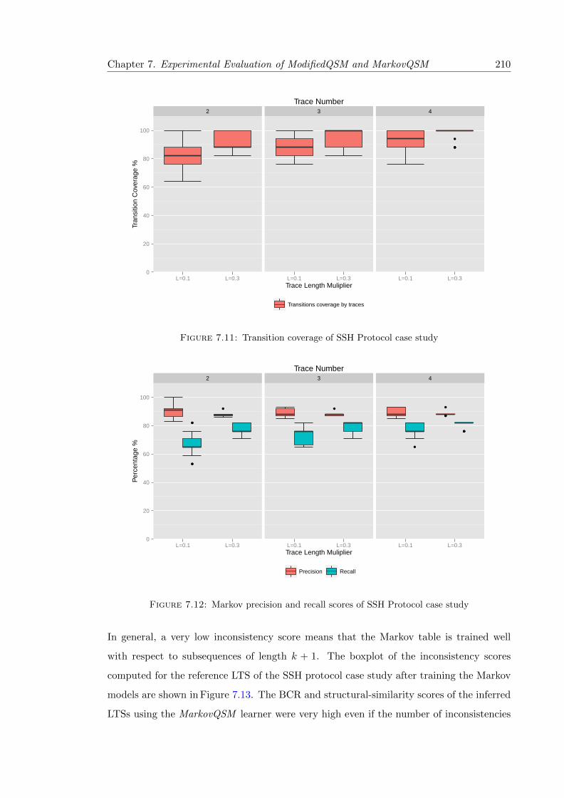
Chapter 7. Experimental Evaluation of ModifiedQSM and MarkovQSM 210
2 3 4
0
20
40
60
80
100
L=0.1 L=0.3 L=0.1 L=0.3 L=0.1 L=0.3Trace Length Muliplier
Tran
sitio
n C
over
age
%
Transitions coverage by traces
Trace Number
Figure 7.11: Transition coverage of SSH Protocol case study
2 3 4
0
20
40
60
80
100
L=0.1 L=0.3 L=0.1 L=0.3 L=0.1 L=0.3Trace Length Muliplier
Per
cent
age
%
Precision Recall
Trace Number
Figure 7.12: Markov precision and recall scores of SSH Protocol case study
In general, a very low inconsistency score means that the Markov table is trained well
with respect to subsequences of length k + 1. The boxplot of the inconsistency scores
computed for the reference LTS of the SSH protocol case study after training the Markov
models are shown in Figure 7.13. The BCR and structural-similarity scores of the inferred
LTSs using the MarkovQSM learner were very high even if the number of inconsistencies

Chapter 7. Experimental Evaluation of ModifiedQSM and MarkovQSM 211
was higher than 10. This is attributed to the idea of asking queries on the condition that
the Im score is higher than the EDSM score. Therefore, whenever the Im score exceeds
the EDSM score, merging of two states is checked using membership queries.
2 3 4
0
2
4
6
8
10
12
14
16
18
20
22
24
26
L=0.1 L=0.3 L=0.1 L=0.3 L=0.1 L=0.3Trace Length Muliplier
Num
ber
of in
cons
iste
ncie
s
Markov
Trace Number
Figure 7.13: Inconsistencies of SSH protocol case study
7.3.2 Case Study: Mine Pump
Figure 7.14 depicts the BCR scores of the inferred LTSs using MarkovQSM, ModifiedQSM
and QSM respectively for the mine pump case study, where different numbers of traces
were considered. In Figure 7.14 there is apparent that MarkovQSM and ModifiedQSM
learners inferred LTSs with higher BCR scores in the majority of cases. The QSM learner,
however, did not learn LTSs well compared to other learners, especially when the num-
ber of traces was below 4. This is because the membership queries posed by the QSM
learner allow bad generalizations of LTSs. In addition, the findings in Figure 7.14 shows
that MarkovQSM and ModifiedQSM inferred models well, and this is because the one-step
queries provide additional information that can prevent the merging of inequivalent pairs
of states. Additionally, QSM generated LTSs well when the number of traces was four
and l = 0.3, unlike if it was two or three.
Table 7.14 reports the p-values of BCR scores obtained from the Wilcoxon signed-rank
statistical test. The considered null hypothesis H0 for this study is that there is no

Chapter 7. Experimental Evaluation of ModifiedQSM and MarkovQSM 212
2 3 4
0.4
0.5
0.6
0.7
0.8
0.9
1.0
L=0.1 L=0.3 L=0.1 L=0.3 L=0.1 L=0.3Trace Length Muliplier
BC
R s
core
MarkovQSM ModifiedQSM QSM
Trace Number
Figure 7.14: BCR scores of water mine pump case study
significant difference between the BCR scores of the inferred LTS using learners. When
comparing ModifiedQSM and QSM in terms of the BCR scores, the H0 can be rejected,
indicating that there is a statistically significant difference between them. However, if the
number of traces is four and l = 0.3, there is no statistically significant difference between
ModifiedQSM and QSM since the p-value exceeded the significance level (0.05). This is
noticeable as the mean value of the BCR scores of the inferred models using ModifiedQSM
and QSM are the same. TheH0 that stated there is no difference between the ModifiedQSM
and MarkovQSM learners is accepted because the p-values are larger than 0.05.
lTrace Number
2 3 4
0.1
ModifiedQSM vs. QSM 8.58× 10−06 2.70× 10−04 0.001
MarkovQSM vs. QSM 1.27× 10−05 1.84× 10−04 0.001
ModifiedQSM vs. MarkovQSM 1 1 1
0.3
ModifiedQSM vs. QSM 0.003 0.008 0.37
MarkovQSM vs. QSM 0.001 0.008 1
ModifiedQSM vs. MarkovQSM 0.34 − 1
Table 7.14: p-values of the Wilcoxon signed-rank test of BCR scores for water minecase study

Chapter 7. Experimental Evaluation of ModifiedQSM and MarkovQSM 213
2 3 4
0.0
0.1
0.2
0.3
0.4
0.5
0.6
0.7
0.8
0.9
1.0
L=0.1 L=0.3 L=0.1 L=0.3 L=0.1 L=0.3Trace Length Muliplier
stru
ctur
al s
imila
rity
scor
e
MarkovQSM ModifiedQSM QSM
Trace Number
Figure 7.15: Structural-similarity scores of water mine pump case study
Figure 7.15 illustrates boxplots of the structural-similarity scores of the mined LTSs
using MarkovQSM, ModifiedQSM and QSM respectively. The outcomes that are shown
in Figure 7.15 demonstrate that the ModifiedQSM and MarkovQSM learners can infer
LTSs with higher structural-similarity scores compared to QSM for the water mine pump
case study. It is noticed that QSM performed well if l = 0.3 since the generated traces
cover more paths in the reference graph compared to l = 0.1. However, both MarkovQSM
and ModifiedQSM inferred good LTSs compared to QSM even if l = 0.1 .
lTrace Number
2 3 4
0.1
ModifiedQSM vs. QSM 5.70× 10−04 0.04 0.02
MarkovQSM vs. QSM 5.12× 10−04 0.03 0.01
ModifiedQSM vs. MarkovQSM 1 1 1
0.3
ModifiedQSM vs. QSM 0.003 0.008 0.37
MarkovQSM vs. QSM 0.001 0.008 1
ModifiedQSM vs. MarkovQSM 0.34 Nan 1
Table 7.15: p-values of Wilcoxon signed rank test of water mine case study for structural-similarity Scores

Chapter 7. Experimental Evaluation of ModifiedQSM and MarkovQSM 214
Table 7.15 summarizes the p-values obtained from the Wilcoxon signed-rank statistical
test after comparing the structural-similarity scores attained by different learners. In this
context, the null hypothesis H0 is stated as the structural-similarity scores of the inferred
models using the two learners are identical. When comparing ModifiedQSM and QSM, the
test reported p-values less than 0.05, and this led to the H0 being rejected, which means
that ModifiedQSM inferred models with higher structural-similarity scores. With the null
hypothesis H0 which stated ModifiedQSM and MarkovQSM learners infer models with the
same structural-similarity scores, it can be accepted since the p-values are greater than
0.05; this proves that there is no significant difference between the structural-similarity
scores of both learners.
T=2 T=3 T=4
20
40
60
30
40
50
60
70
30
40
50
60
70
L=0.1 L=0.3 L=0.1 L=0.3 L=0.1 L=0.3Trace Number
num
ber
of m
embe
rshi
p qu
erie
s
MarkovQSM ModifiedQSM QSM
Tracenumber
Figure 7.16: The number of membership queries of different learners for water minecase studt
Figure 7.16 shows the number of membership queries that were asked by various algo-
rithms. Clearly, ModifiedQSM and MarkovQSM learners asked queries more than QSM
as illustrated in Figure 7.16. Despite the similarity between MarkovQSM and Modi-
fiedQSM in terms of the BCR and structural-similarity scores, the MarkovQSM learner
asked fewer membership queries compared to ModifiedQSM when L = 0.3, due to the
idea that MarkovQSM asks membership queries if the Im score is higher than the EDSM
score. Moreover, the number of membership queries that posed using the MarkovQSM
learner was 8.2% less than those posed using ModifiedQSM when l = 0.3. Thus, a possible

Chapter 7. Experimental Evaluation of ModifiedQSM and MarkovQSM 215
explanation for this reduction might be that the collected traces does not cover paths in
the reference LTS well.
It is important to assess the performance of the proposed algorithms in terms of the num-
ber of membership queries posed to the oracle. As shown in Figure 7.16, QSM asked fewer
queries than other learners. Table 7.16 provides summary of the p-values obtained from
the Wilcoxon signed-rank statistical test for the number of membership queries. The null
hypothesis H0 is stated as the number of membership queries posed by the learners are
the same. The test reported p-values less than 0.05 when comparing ModifiedQSM and
QSM. In this case, the H0 is rejected, which means that ModifiedQSM consumed more
queries as shown in Figure 7.16. With the number of traces three or four, the null hypoth-
esis H0 which stated ModifiedQSM and MarkovQSM learners posed the same number of
membership queries can be rejected since the p-values are greater than 0.05; this means
that MarkovQSM asked fewer queries compared to ModifedQSM.
lTrace Number
2 3 4
0.1
ModifiedQSM vs. QSM 1.79× 10−06 1.75× 10−06 1.72× 10−06
MarkovQSM vs. QSM 1.73× 10−06 1.74× 10−06 1.76× 10−06
ModifiedQSM vs. MarkovQSM 0.95 0.49 0.09
0.3
ModifiedQSM vs. QSM 1.80× 10−06 1.78× 10−06 1.78× 10−06
MarkovQSM vs. QSM 1.80× 10−06 1.79× 10−06 1.78× 10−06
ModifiedQSM vs. MarkovQSM 0.15 1.56× 10−04 1.82× 10−05
Table 7.16: p-values obtained by the Wilcoxon signed-rank test of number of member-ship queries for water mine case study
Figure 7.17 shows the percentage of transitions that were covered by the traces in the
conducted experiments for this case study. It turned out that the QSM learner performed
poorly when the generated traces did not visit all transitions. It is important to highlight
that ModifiedQSM and MarkovQSM performed better than OSM if the transition cover
was 80%. It was noticed early in this section, the BCR scores achieved by MarkovQSM
when l = 0.1 were lower than the attained scores when l = 0.3. This is because the
transition cover increased when l = 0.3 in comparison with l = 0.1, as seen in Figure 7.17.

Chapter 7. Experimental Evaluation of ModifiedQSM and MarkovQSM 216
2 3 4
0
20
40
60
80
100
L=0.1 L=0.3 L=0.1 L=0.3 L=0.1 L=0.3Trace Length Muliplier
Tran
sitio
n C
over
age
%
Transitions coverage by traces
Trace Number
Figure 7.17: Transition coverage of water mine case study
2 3 4
0
20
40
60
80
100
L=0.1 L=0.3 L=0.1 L=0.3 L=0.1 L=0.3Trace Length Muliplier
Per
cent
age
%
Precision Recall
Trace Number
Figure 7.18: Markov precision and recall scores of water mine case study
Figure 7.18 shows the precision/recall scores of the trained Markov models for various
numbers of traces that were considered in the conducted experiments. The precision
scores of the trained Markov model were above 0.80, and this led to the detection of

Chapter 7. Experimental Evaluation of ModifiedQSM and MarkovQSM 217
inconsistencies whenever state merges were performed. However, the recall is very low
when the number of traces is two and l=0.1 since the transitions were not covered well in
this case, as shown in Figure 7.17.
2 3 4
0
2
4
6
8
10
12
14
16
L=0.1 L=0.3 L=0.1 L=0.3 L=0.1 L=0.3Trace Length Muliplier
Num
ber
of in
cons
iste
ncie
s
Markov
Trace Number
Figure 7.19: Inconsistencies of water mine case study
During the conducted experiment, it was interesting to compute the number of inconsis-
tencies with respect to the reference LTS. Figure 7.19 shows the number of inconsistencies
that were found in the reference LTS based on the trained Markov models. The idea behind
computing the inconsistency score for the reference graph is to measure how accurately
the MarkovQSM learner can detect inconsistencies. In addition, there is a relationship
between the number of inconsistencies computed for the reference model based on the
trained Markov model and the performance of the learners. One may notice that the
highest BCR scores of the inferred models using QSM happens when the collected traces
cause the smallest inconsistencies.
7.3.3 Case Study: CVS Client
The BCR scores of the mined LTSs using different algorithms are shown in Figure 7.20.
ModifiedQSM learned LTSs with better BCR scores compared to other learners. Moreover,
the BCR scores of the inferred LTSs using the MarkovQSM learner were not good enough
as ModifiedQSM, especially when L = 0.3. When the number of traces were three and
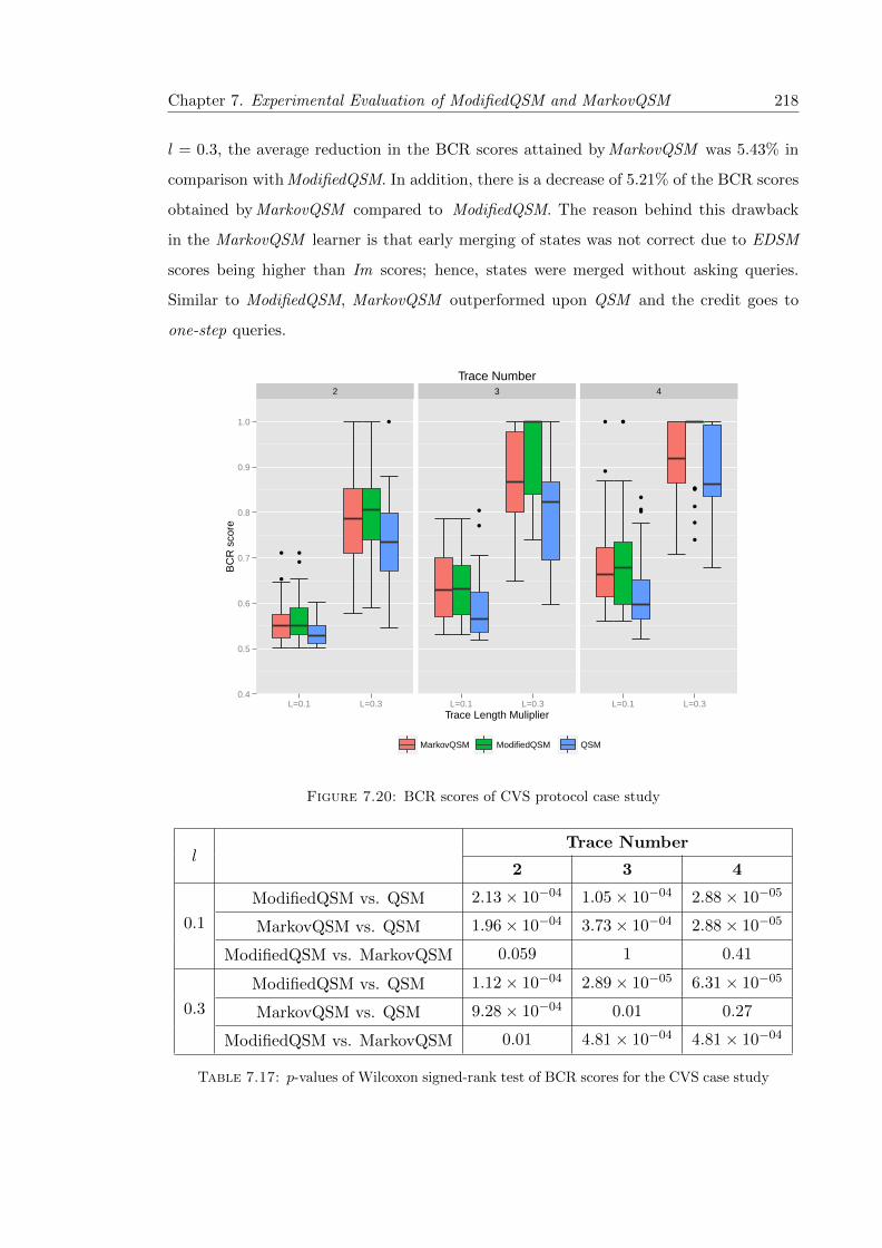
Chapter 7. Experimental Evaluation of ModifiedQSM and MarkovQSM 218
l = 0.3, the average reduction in the BCR scores attained by MarkovQSM was 5.43% in
comparison with ModifiedQSM. In addition, there is a decrease of 5.21% of the BCR scores
obtained by MarkovQSM compared to ModifiedQSM. The reason behind this drawback
in the MarkovQSM learner is that early merging of states was not correct due to EDSM
scores being higher than Im scores; hence, states were merged without asking queries.
Similar to ModifiedQSM, MarkovQSM outperformed upon QSM and the credit goes to
one-step queries.
2 3 4
0.4
0.5
0.6
0.7
0.8
0.9
1.0
L=0.1 L=0.3 L=0.1 L=0.3 L=0.1 L=0.3Trace Length Muliplier
BC
R s
core
MarkovQSM ModifiedQSM QSM
Trace Number
Figure 7.20: BCR scores of CVS protocol case study
lTrace Number
2 3 4
0.1
ModifiedQSM vs. QSM 2.13× 10−04 1.05× 10−04 2.88× 10−05
MarkovQSM vs. QSM 1.96× 10−04 3.73× 10−04 2.88× 10−05
ModifiedQSM vs. MarkovQSM 0.059 1 0.41
0.3
ModifiedQSM vs. QSM 1.12× 10−04 2.89× 10−05 6.31× 10−05
MarkovQSM vs. QSM 9.28× 10−04 0.01 0.27
ModifiedQSM vs. MarkovQSM 0.01 4.81× 10−04 4.81× 10−04
Table 7.17: p-values of Wilcoxon signed-rank test of BCR scores for the CVS case study

Chapter 7. Experimental Evaluation of ModifiedQSM and MarkovQSM 219
A summary of statistical analysis for the CVS case study is given in Table 7.17 where
the p-values resulted from comparing BCR scores. In this study, the considered null hy-
pothesis H0 stated that the BCR scores of any two learners are the same. The p-values
obtained by comparing the BCR scores of ModifiedQSM and QSM suggested rejection
of the H0 since the p-values were less than 0.05, and this indicates that there is a sta-
tistically significant difference between both learners. This means that the BCR scores
attained by ModifiedQSM were higher than QSM as shown in Figure 7.20. When com-
paring MarkovQSM and QSM when l = 0.1, the p-values were too small and showed a
statistically significant difference between both learners. In other words, the performance
of MarkovQSM was better than QSM. However, when the number of traces is four and
l = 0.3, MarkovQSM did not perform better than QSM since the p-value was 0.27. The
p-values were above 0.05 when l = 0.1 when comparing the BCR scores of ModifiedQSM
and MarkovQSM learners, indicating that there was no significant difference between the
two learners. Moreover, the Wilcoxon p-values were below 0.05 when l = 0.3, implying
that ModifiedQSM inferred LTSs with better BCR scores compared to MarkovQSM.
2 3 4
0.0
0.1
0.2
0.3
0.4
0.5
0.6
0.7
0.8
0.9
1.0
L=0.1 L=0.3 L=0.1 L=0.3 L=0.1 L=0.3Trace Length Muliplier
stru
ctur
al s
imila
rity
scor
e
MarkovQSM ModifiedQSM QSM
Trace Number
Figure 7.21: Structural-similarity scores of CVS protocol case study
Figure 7.21 depicts the structural-similarity scores of the inferred LTSs using MarkovQSM,
ModifiedQSM, and QSM respectively for the CVS case study. From the boxplots that are

Chapter 7. Experimental Evaluation of ModifiedQSM and MarkovQSM 220
shown in Figure 7.21, it is apparent that ModifiedQSM generated LTSs models with the
highest structural-similarity scores compared to other learners. In addition, the structural-
similarity scores achieved by MarkovQSM was not good, as compared with the structural-
similarity scores of the inferred models using ModifiedQSM. It is worth mentioning that
the structural-similarity scores of the inferred LTSs using QSM were much lower than
those attained by other learners. This proves that membership queries asked by QSM are
insufficient to learn LTSs well.
Table 7.18 summarizes the p-values that resulted from the Wilcoxon signed-rank statistical
test after comparing the structural-similarity scores of learners. The null hypothesis H0
is that the structural-similarity scores of the learners are the same. The H0 is rejected
when comparing ModifiedQSM and QSM because the p-value is less than 0.05, and this is
a strong evidence that there is a statistically significant difference between both learners.
Moreover, when comparing structural-similarity scores obtained by MarkovQSM and QSM
learners, the p-values show that there is a significant difference between both learners when
l = 0.1. However, the H0 is accepted when l = 0.3 and the number of traces are four;
this means that the performance of MarkovQSM and QSM are the same in terms of the
structural-similarity scores as shown in Figure 7.21.
lTrace Number
2 3 4
0.1
ModifiedQSM vs. QSM 4.00× 10−06 4.00× 10−06 2.70× 10−06
MarkovQSM vs. QSM 6.18× 10−06 1.16× 10−05 2.70× 10−06
ModifiedQSM vs. MarkovQSM 0.059 0.016 0.04
0.3
ModifiedQSM vs. QSM 1.03× 10−05 1.82× 10−06 2.64× 10−06
MarkovQSM vs. QSM 0.06 0.049 0.25
ModifiedQSM vs. MarkovQSM 1.30× 10−04 8.69× 10−06 1.92× 10−05
Table 7.18: p-values of Wilcoxon signed rank test of CVS case study for structural-similarity scores
The number of membership queries that were submitted to the oracle using various al-
gorithms is shown in Figure 7.22. As the figure demonstrates, the MarkovQSM learner
asked fewer queries compared to ModifiedQSM when l = 0.3. This demonstrates that the
EDSM scores were higher than the Im scores, and this led to queries being skipped, which
was not accurate. It is worth mentioning that ModifiedQSM and MarkovQSM learners

Chapter 7. Experimental Evaluation of ModifiedQSM and MarkovQSM 221
asked more queries than QSM, as illustrated in Figure 7.22. There is a slight decline of
1.71% of the average of numbers of membership queries posed by MarkovQSM compared
to ModifiedQSM when l = 0.3 and the number of traces is two. In addition, when the
number of traces is three, the number of membership queries asked by the MarkovQSM
learner was decreased by 12.04% compared to ModifiedQSM.
T=2 T=3 T=4
100
200
300
100
200
300
400
100
200
300
400
L=0.1 L=0.3 L=0.1 L=0.3 L=0.1 L=0.3Trace Number
num
ber
of m
embe
rshi
p qu
erie
s
MarkovQSM ModifiedQSM QSM
Tracenumber
Figure 7.22: The number of membership queries of different learners for water minecase study
It is vital to determine whether any of the learners asked fewer queries than other learners.
Table 7.19 provides a summary of the p-values obtained from the Wilcoxon signed-rank
statistical test for the number of membership queries. The null hypothesis H0 is stated as
the number of membership queries posed by the learners are the same. The test reported
p-values less than 0.05 when comparing ModifiedQSM and QSM. In this case, the H0 is
rejected, which means that ModifiedQSM consumed more queries, as shown in Figure 7.22.
With l = 0.3, the null hypothesis H0 which stated ModifiedQSM and MarkovQSM learners
posed the same number of membership queries can be rejected if the number of traces is
four; this means that there is strong evidence MarkovQSM asked fewer queries compared
to ModifedQSM. However, there is no significant difference between the ModifiedQSM and
MarkovQSM learners in terms of the number of membership queries when the number of
traces is three since the p-values > 0.05.

Chapter 7. Experimental Evaluation of ModifiedQSM and MarkovQSM 222
lTrace Number
2 3 4
0.1
ModifiedQSM vs. QSM 1.82× 10−06 2.23× 10−06 1.82× 10−06
MarkovQSM vs. QSM 1.82× 10−06 2.47× 10−06 2.02× 10−06
ModifiedQSM vs. MarkovQSM 0.01 0.31 6.53× 10−04
0.3
ModifiedQSM vs. QSM 6.89× 10−04 3.72× 10−05 3.44× 10−04
MarkovQSM vs. QSM 0.006 0.012 0.018
ModifiedQSM vs. MarkovQSM 0.048 0.34 0.002
Table 7.19: p-values obtained by the Wilcoxon signed-rank test of numbers of queriesfor CVS case study
2 3 4
0
20
40
60
80
100
L=0.1 L=0.3 L=0.1 L=0.3 L=0.1 L=0.3Trace Length Muliplier
Tran
sitio
n C
over
age
%
Transitions coverage by traces
Trace Number
Figure 7.23: Transition coverage of CVS case study
Figure 7.23 shows the transition coverage that was computed based on the traces in the
conducted experiments for this case study. It is obvious that only the ModifiedQSM learner
performed well when not all transitions were visited by the generated traces. On the
other hand, the performance of QSM was worse than both ModifiedQSM and MarkovQSM
learners.
The precision and recall scores of the trained Markov models computed for all traces
considered in the conducted experiments are illustrated in Figure 7.24. The precision

Chapter 7. Experimental Evaluation of ModifiedQSM and MarkovQSM 223
scores of the trained Markov model were above 100% and this led to accurate predictions
being made. However, many predictions were missed since the recall was very low when
l = 0.1 and the transitions were not covered well in this case as shown in Figure 7.23.
The performance of MarkovQSM was not affected by the low value of the recall since
MarkovQSM asks queries whenever the Im score exceeds the EDSM.
2 3 4
0
20
40
60
80
100
L=0.1 L=0.3 L=0.1 L=0.3 L=0.1 L=0.3Trace Length Muliplier
Per
cent
age
%
Precision Recall
Trace Number
Figure 7.24: Markov precision and recall scores of CVS case study
The number of inconsistencies computed for the reference LTS of CVS case study after
training Markov models are illustrated in Figure 7.25. It is obvious that the number of
inconsistencies was high when l = 0.1, and this meant that the MarkovQSM learner did
not skip asking membership queries during the early mergers of states.
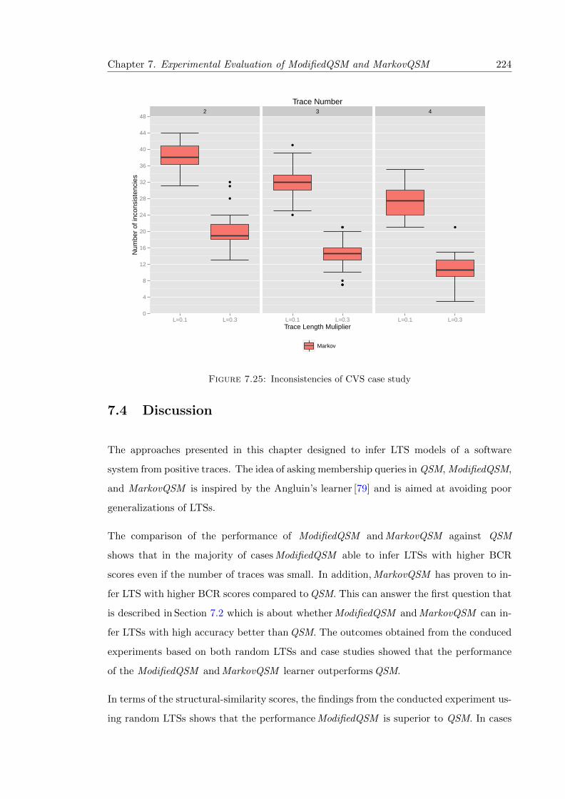
Chapter 7. Experimental Evaluation of ModifiedQSM and MarkovQSM 224
2 3 4
0
4
8
12
16
20
24
28
32
36
40
44
48
L=0.1 L=0.3 L=0.1 L=0.3 L=0.1 L=0.3Trace Length Muliplier
Num
ber
of in
cons
iste
ncie
s
Markov
Trace Number
Figure 7.25: Inconsistencies of CVS case study
7.4 Discussion
The approaches presented in this chapter designed to infer LTS models of a software
system from positive traces. The idea of asking membership queries in QSM, ModifiedQSM,
and MarkovQSM is inspired by the Angluin’s learner [79] and is aimed at avoiding poor
generalizations of LTSs.
The comparison of the performance of ModifiedQSM and MarkovQSM against QSM
shows that in the majority of cases ModifiedQSM able to infer LTSs with higher BCR
scores even if the number of traces was small. In addition, MarkovQSM has proven to in-
fer LTS with higher BCR scores compared to QSM. This can answer the first question that
is described in Section 7.2 which is about whether ModifiedQSM and MarkovQSM can in-
fer LTSs with high accuracy better than QSM. The outcomes obtained from the conduced
experiments based on both random LTSs and case studies showed that the performance
of the ModifiedQSM and MarkovQSM learner outperforms QSM.
In terms of the structural-similarity scores, the findings from the conducted experiment us-
ing random LTSs shows that the performance ModifiedQSM is superior to QSM. In cases

Chapter 7. Experimental Evaluation of ModifiedQSM and MarkovQSM 225
where m > 0.5, ModifiedQSM shows a slight improvement compared to MarkovQSM in
terms of structural-similarity scores. This is due to the MarkovQSM learner find inconsis-
tencies accurately, and allows asking membership queries when Im scores exceeds EDSM
scores.
The efficiency in the performance of MarkovQSM against ModifiedQSM shows that both
learners can infer LTSs with very similar BCR and structural-similarity scores when
m = 2.0. This is due to the high precision value of the trained Markov model. In this
case, MarkovQSM allowing merging states without asking membership queries accurately
compared to the cases where m < 2.0. Therefore, it appears that the performance of the
MarkovQSM learner depends on the accuracy of the trained Markov model.
It was noticed during the conducted experiments that the ModifiedQSM algorithm asked
more queries compared to other algorithms. Since both ModifiedQSM and MarkovQSM
asks membership queries using the Dupont and one-step generators, it is expected to ask
more membership queries compared to the QSM learner. Although ModifiedQSM and MarkovQSM
asked membership queries more than QSM, they inferred LTSs with higher accuracy. This
is due to the extra check made by the one-step queries that help the ModifiedQSM and
MarkovQSM learners to prevent bad state merges during the inference process.
Another important finding was that MarkovQSM able to reduce the number of member-
ship queries submitted to the oracle compared to ModifiedQSM. For the conducted exper-
iment using random LTSs, MarklovQSM has shown to reduce the number of membership
queries with slight losing in the accuracy of the inferred LTSs when m = 1.0 or 2.0. Sur-
prisingly, for water mine pump and SSH case studies, MarkovQSM performed very similar
to ModifiedQSM. Moreover, MarkovQSM asked fewer queries compared to ModifiedQSM
in both case studies, especially when l = 0.3. This is because the initial Markov models
were trained with enough traces. Hence, MarkovQSM was able to skip asking membership
queries accurately.
To conclude, the conducted experiment has proven that the quality of the inferred LTS can
be improved using the concept of active learning. Walkinshaw and Bogdanov [45] stated
that the QSM learner can infer an accurate LTSs if the provided traces is structurally
complete (see Definition 2.10). Sometimes, the ModifiedQSM learner can infer a correct
automaton even if the traces are not structurally complete. Therefore, it is important to

Chapter 7. Experimental Evaluation of ModifiedQSM and MarkovQSM 226
emphasize that the ModifiedQSM learner is able to infer learn a correct automaton if they
ask queries that prevent bad mergers.
7.5 Threats to Validity
1. The randomly generated LTSs may not represent real-world models.
This threat is mitigated by evaluating the performance of ModifiedQSM and MarkovQSM
on case studies that are used in the literature review and the survey of stamina com-
petition [35].
2. The selection of training data may not be representative .
One possible threat to validity is the selection of training data where they might
not be representative. For random LTSs, this threat is mitigated against it, each
LTS was attempted to infer 5 times with different paths generated each time since
random traces may follow the same paths many times. When the performance of
ModifiedQSM and MarkovQSM were evaluated on case studies, 30 different sets of
random traces were used in order to mitigate this threat.
3. The size of case studies may not representative of all state machines. One
possible threat to validity is that the sizes of case studies where their sizes are small.
The reason behind evaluating the performance of ModifiedQSM and MarkovQSM
on such case studies are that they are widely used in state machine inference papers.
4. The parameters settings could bias the results. In the conducted experiments,
there are many parameters such as the number of traces, alphabet size, and prefix
length. Another possible threat to validity is that the variance of such parameters
may bias the results. This threat is mitigated by choosing a different multiplier
to vary the parameters. For instance, the alphabet multiplier m intended to vary
the alphabet size to assess the performance of ModifiedQSM and MarkovQSM on
different types of LTSs. In addition, different number of traces were selected to assess
the performance of the proposed algorithms.

Chapter 7. Experimental Evaluation of ModifiedQSM and MarkovQSM 227
7.6 Conclusion
This chapter evaluates ModifiedQSM and MarkovQSM learners. The performance of
the ModifiedQSM was evaluated using randomly generated LTSs and case studies, the
outcomes showing that despite the cost of the number of membership queries was high,
the accuracy of the inferred LTSs was improved significantly.
On the other hand, the MarkovQSM learner showed its ability to improve the accuracy
of the inferred LTSs compared to QSM. Moreover, the computation of inconsistencies can
aid the MarkovQSM learner to reduce the cost of membership queries that are asked
by ModifiedQSM. However, the performance of MarkovQSM is limited when the alphabet
size is not very high.

8Conclusion and Future Work
8.1 Introduction
Inferring state-machine models is an approach to supporting verification and validation
techniques that is gaining interest among software engineers. The existing inference tech-
niques suffer from a poor ability to infer good models when only positive traces are avail-
able. This thesis has focused on the inference of LTS models in cases where the negative
traces are sparse or completely missing. In this research, new LTS learning algorithms have
been proposed to improve the existing ones. The first inference algorithm relies on the
idea of heuristic-based state merging representing in the EDSM learner and the trained
Markov models to work together to prevent bad generalization of models. The second
learning algorithm utilizes the idea of active learning to overcome bad generalization of
LTSs, which is named ModifiedQSM. The third inference algorithm is called MarkovQSM,
which is an extension to ModifiedQSM. MarkovQSM depends on information extracted
228

Chapter 8. Conclusion and Future Work 229
from the Markov models to reduce the number of membership queries consumed by other
learners.
8.2 Summary of Thesis and Achievements
The introduction to the thesis is described in Chapter 1, including the motivation and
problem of the thesis. In addition, it provides an overview of the problem of specification
inference and its impact on verification and validation techniques. Chapter 2 introduced
the definitions and notations related to LTS models. Besides, it includes introduction
to LTS learning in terms of state merging strategy. Chapter 2 addressed the ways of
evaluating state-machine inference techniques from different perspectives, providing the
evolution framework used in this thesis.
Chapter 3 described the existing inference techniques that rely on state merging and
identified problems to be solved in the following chapters. In addition, it provides other
relevant research studies of LTS inference.
Chapter 4 and Chapter 5 demonstrated the possibility of using the Markov model alongside
the EDSM learner to help the inference process in order to infer good LTS models. This
combination technique is called EDSM-Markov, which is described in Chapter 4. In addi-
tion to this, ways to evaluate the correctness of the trained Markov models are described
using the precision and recall.
The quality of the inferred LTSs by EDSM-Markov was compared to SiccoN inference using
metrics, and it was shown to obtain reasonable results (see Chapter 5) in the majority of
cases. Although inferring good LTSs using the EDSM-Markov learner was achieved when
the size of the alphabet was large. However, there were different cases that did not achieve
good BCR scores such as where |Σ| = 0.5× |Q|.
Chapter 6 proposed two different LTS inference algorithms that aimed to improve per-
formance of the QSM learner [36] to infer better LTSs. The efficiency of ModifiedQSM
and MarkovQSM learners was evaluated as demonstrated in Chapter 7. to measure
the capability of both learners using different randomly-generated LTSs and case stud-
ies. The outcomes from the experimental evaluation can be summarized by saying that

Chapter 8. Conclusion and Future Work 230
the ModifiedQSM learner outperformed other learners in terms of the quality of the in-
ferred LTSs, however it also asked more membership queries. The MarkovQSM learner
has been proven to reduce the number of membership queries compared to ModifiedQSM.
8.3 Contributions
The study in this thesis has focused on the well-known problem of inferring LTSs from
only positive traces and introduced improvements to the existing state-merging inference
algorithms. The present study contributes evidence that suggests that the inference of
LTSs can benefit from a predictive model in order to overcome difficulties of inferring
LTSs from positive traces only.
The EDSM-Markov learner makes it possible to improve an existing EDSM inference
method in the context of LTSs encountered in software models. As stated in Chapter 1,
passive state-machine learning based on the state-merging strategy is known to cause over-
generalization, especially if the provided traces are sparse or negative traces are insufficient
to prevent over-generalization. The empirical finding in this thesis showed that it is possi-
ble to reduce the problem of over-generalization. This is based on building Markov models
that can then be used in a scoring heuristic, permitting effective learning from a few en-
tirely positive traces. It has proven to perform well for learning LTSs when the alphabet
size is very large.
One of the important contributions of the described work is that the EDSM-Markov learner
has the ability to assess its own performance. Where the inconsistency score computed
for an inferred LTS is very different to the one computed for the reference LTS based on
the initial PTA (Traces), this usually indicates that the inferred graph is very far from
what might be expected. Furthermore, in the conducted experiment with random LTSs,
if the inconsistency score computed for the initial models was above a few hundred, this
indicates that the EDSM-Markov learner has to collect more traces.
Interestingly, the empirical findings in this thesis provide a new route of investigating using
an inconsistency measurement as a coverage metric for a training set. This is based on
the experimental observation that where an inconsistency of a reference graph based on
training data is above 100, it is unlikely that such training data will be useful in inference.

Chapter 8. Conclusion and Future Work 231
The present study in Chapter 7 contains several contributions to the original QSM learner.
It extends the membership queries by proposing new generator of queries that are designed
to avoid bad state mergers. In addition, both ModifiedQSM and MarkovQSM learners
avoid restarting the learning process of an LTS in the original QSM that was proposed
by Dupont et al. [36]. The findings of using the inconsistency computation to the concept of
active learning contributes additional evidence that the number of queries can be reduced.
This is represented in the MarkovQSM learner described in Chapter 7.
8.4 Research Questions
1. How effective are Markov models at capturing dependencies between
events in realistic software?
The precision scores of the trained Markov models indicates how correctly they can
capture dependencies between events that appeared in the provided traces. Dur-
ing the conducted experiments, the precision scores were high if the alphabet size
was large, denoting that Markov models can capture dependencies between events
appears in traces.
2. How effective are Markov models as a source of prohibited events in the
inference of models from realistic software using EDSM ?
The use of Markov models to compute inconsistencies during the inference has been
shown to aid the state-merging strategy to avoid bad mergers. Thus, events that
are predicted as prohibited to follow a sequence of events of length k can be used to
detect inconsistencies accurately. Events that are not predicted either as permitted
or prohibited by a Markov model can be used as a source of prohibited events if the
generated traces cover transitions well. The evaluation of the EDSM-Markov learner
proved that it benefits from computing inconsistencies based on such prohibited
events. It was clear that the accuracy of the inferred LTSs models the EDSM-Markov
learner was increased, and this was because inconsistencies were detected correctly.
3. Under which conditions does EDSM with Markov models improve over
EDSM without Markov models?
The findings in the experiments demonstrate that inferring LTSs using EDSM-Markov
can achieve good results if the traces are covering the system being inferred well. In

Chapter 8. Conclusion and Future Work 232
addition, it was obvious that the quality of the inferred models is improved when
the alphabet size is very large. The proposed heuristic that relies upon the Markov
models helps the EDSM-Markov learner to identify inconsistencies resulting from
merging states. Those inconsistencies showed to help in blocking invalid mergers of
states.
The precision of the trained Markov model plays a vital role in detecting inconsis-
tencies during the state merging process. In cases where the precision scores of the
trained Markov models are small, the EDSM-Markov learner fails to collect incon-
sistencies, and this leads to merge states that should not be merged. Hence, the
improvements were not good if the precision scores of the trained Markov models
were small.
4. To what extent are the developed inference algorithms able to generate
exact models and avoid over-generalization problem?
Inferring the exact models from only positive traces is difficult [56]. The developed
inference method that passively infers LTS models showed that obtaining the exact
model still hard to be accomplish. In some cases, the experimental outcomes proved
that it is possible to infer the exact model on the condition that the provided positive
traces covering the system well and the alphabet size is very large.
Besides this, over-generalization is a well-known problem that is encountered in the
domain of grammar inference and specification mining in a wider context. Over-
generalization occurs in case of learning from only positive training data [52, 145,
146]. The investigation in this thesis demonstrates that the problem of over-generalization
can be reduced either using the IScore heuristic or utilizing active learning, which is
more costly because it relies membership queries.
5. Under which conditions does QSM with Markov models improve over
QSM without Markov models?
The outcomes from the conducted experiments showed that inferring LTSs using MarkovQSM
can improve over QSM if the alphabet size is large. This is due to the precision of the
trained Markov models being high enabling identification of questionable mergers.
In cases where alphabet size is very large, the BCR scores of the inferred LTS using
MarkovQSM were higher than those obtained using QSM.

Chapter 8. Conclusion and Future Work 233
6. With respect to the concept of active inference, what is the reduction of
the number of queries obtained by using Markov models, compared to
QSM ?
Since the concept of active learning was proposed by Angluin [79], researchers have
worked on reducing the number of queries submitted to the oracle. Unfortunately,
the ModifiedQSM learner has proven to ask more queries compared to the QSM
learner. This is intuitive and it is possible to say that gaining an improvement re-
garding the accuracy of the inferred models takes more effort in terms of the number
of asked queries.
8.5 Limitations and Future Work
One of the major limitations of the present study is that the idea of finding inconsisten-
cies based on the Markov models is not suitable for learning LTSs with small alphabets.
Another limitation of the proposed learner that relies on the concept of passive learning
(EDSM-Markov) is the collection of traces. Where achieving high-approximation LTSs is
not an easy task, the performance of EDSM-Markov learner is limited if the number of
traces is small or they did not cover the system under inference. Further improvements
can be introduced in the future work as will be described in Section 8.5.1.
Another weakness in the proposed techniques that rely on the concept of active learning
is that the exact identification of LTS models is difficult if the number of traces is very
small; this is because the performance of those techniques depends on the provided traces.
Possible improvements can be made to improve the quality of the inferred LTSs and to
reduce the number of membership queries submitted to an oracle.
8.5.1 Possible Improvements to EDSM-Markov
Future work could aims to improve the inference technique in terms of the accuracy of
their outcomes. For instance, one may use Markov models to predict labels of transitions
leaving a state, based on other sequences of labels of outgoing transitions leaving the same
state, or predicting labels of incoming transitions based on the existence of outgoing ones.

Chapter 8. Conclusion and Future Work 234
A significant part of future work will be making it easy to adjust heuristical scoring for
specific kinds of automata. In addition, experiments of the EDSM-Markov learner showed
that it was not easy to find the right balance between the EDSM score and Im score. One
direction of future improvement is to use the inconsistency score as an estimator to identify
pairs of states that cause the smallest inconsistency to give them preference to be merged
first.
A future study could investigate starting the inference process using merging states not
from the root but anywhere in a PTA. The aim is to avoid the problem of early mergers
where limited choices of pair of states exist to pick the best one. This may be achieved
by collecting states that share labels or a sequence of labels of outgoing transitions where
merging such states causes the smallest inconsistencies based on the Im score.
Sometimes, the EDSM-Markov learner fails to find a good LTS even if the computed
inconsistency for the initial PTA is small. Based on a high inconsistency score of the learnt
LTS, the EDSM-Markov learner could then restart the inference process, with different
heuristics or with rules mined from the traces, aiming to reduce the perceived inconsistency.
Finally, it is known that an effective test set can be used to infer a model from which it
was derived, and in a similar way, one possible investigation of future work could be to
see to what extent a measure of inconsistency could be good as a metric reflecting test set
adequacy.
8.5.1.1 Finding Multiple Solutions
The proposed techniques of LTS inference from positive traces presented in this thesis
attempted to infer only one LTS per specific problem to be solved. In their paper [110],
multiple DFA solutions were inferred for each specific inference task. In addition, Heule
and Verwer [110] used an ensemble method [121] to generalize those solutions by finding an
average DFA language. In a similar manner, further research might investigate the possi-
bility of inferring multiple LTSs for each specific inference problem to solve the sparseness
of the traces. Besides, the computation of inconsistency introduced in Chapter 5 can be
used to determine which one of those solutions causes the smallest inconsistency score.
Further studies could examine the relationship between BCR scores and inconsistency
scores. Given multiple LTSs inferred for a specific task, study the following problem:

Chapter 8. Conclusion and Future Work 235
How likely is it that the inferred LTS with the highest BCR score has the
smallest inconsistency scores among other solutions?.
The performance of EDSM-Markov becomes weak if the alphabet size is not too large and
it tends to merge states incorrectly, which yields over-generalized LTSs. Future work may
include introducing more constrains such those used by Heule and Verwer [110].
8.5.1.2 Mining Rules from the Traces
Another method that might be implemented to improve the proposed algorithms is to
incorporate rule-mining techniques with the state-merging strategy. This is inspired by
previous works [70, 138] where mined rules were used to block merging states if there is
a contradiction with these rules. In other words, the mined rules capture dependencies
between events in the collected traces, and the rules which can be used in our context to
block merging of states if any of those rules are violated.
8.5.2 Possible Improvements to ModifiedQSM and MarkovQSM
The idea behind ModifiedQSM and MarkovQSM is to ask the membership queries during
the computation of scores to give preference to states in the pair that are most likely to
be equivalent. Unfortunately, similar to the QSM learner, both learners ModifiedQSM
and MarkovQSM require training data that should have high coverage to infer the exact
models. To avoid the sparseness of the training data, using counterexamples in the same
way that they are used by Angluin [79] can help to overcome the low coverage of training
data. However, this can be challenging because a restart of the learning is required after
each counterexample.
Another line of improvement would be to investigate the effect of re-ordering the list of
membership queries on the number of submitted queries to an oracle. The aim of re-
ordering is to decide which membership queries to ask first, this may reduce the number
of membership queries. To achieve this, a trained Markov model can be used to evaluate
membership queries based upon the appearance of subsequences, where a query that has
the maximum number of subsequences never seen so far will take a higher priority to be
asked first.

Chapter 8. Conclusion and Future Work 236
As described in Chapter 7, in the one-step generator, labels of outgoing transitions leaving
a red state that lead to an accepting state are asked from a blue state. Future work
may include asking membership queries of making two or three steps. A future study
investigating the use of rule-mining techniques to block merging of states before asking
the membership queries would be very interesting.
8.6 Thesis Conclusion
This thesis has investigated the possibility of integrating the concept of Markov models
to the problem of inferring LTSs from positive traces. There are different solutions that
have been introduced to tackle this problem, and their efficiency is assessed using practical
experiments.
The inference of LTS models from only positive traces has been demonstrated to be a hard
task; however, the difficulty can be reduced by searching for further solutions, especially
integrating domain-specific information such as temporal rules. The sparsity of the training
data is known to be a challenge in different domains, and the concept of grammar inference
is one of them. While passive inference methods may be enhanced by improving heuristics
or integrating domain knowledge, the sparsity of training data will be problematic. This
can be tackled using the concept of active inference, but it still needs further investigation
to reduce the cost of asking and answering queries.
AAppendix of inferred model evaluation
A.1 Test sequences generated for the text editor example
In the following table, the test sets that are generated from the reference LTS of the text
editor example. The first column represents the list of tests, the second column repre-
sents the correct classification of each test whether the test is accepted (true) or rejected
(false) by the reference LTS. For each test, the third column represents the corresponding
classification that is obtained from the inferred LTS.
Table A.1: The set of tests and the corresponding classification using the reference LTSand the inferred LTS
Test Reference LTS Inferred LTS
Close false false
Save false false
Continued on next page
237
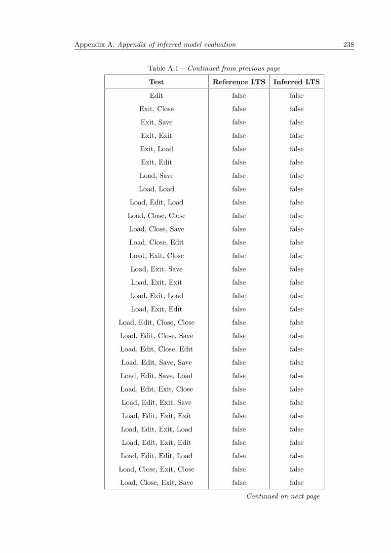
Appendix A. Appendix of inferred model evaluation 238
Table A.1 – Continued from previous page
Test Reference LTS Inferred LTS
Edit false false
Exit, Close false false
Exit, Save false false
Exit, Exit false false
Exit, Load false false
Exit, Edit false false
Load, Save false false
Load, Load false false
Load, Edit, Load false false
Load, Close, Close false false
Load, Close, Save false false
Load, Close, Edit false false
Load, Exit, Close false false
Load, Exit, Save false false
Load, Exit, Exit false false
Load, Exit, Load false false
Load, Exit, Edit false false
Load, Edit, Close, Close false false
Load, Edit, Close, Save false false
Load, Edit, Close, Edit false false
Load, Edit, Save, Save false false
Load, Edit, Save, Load false false
Load, Edit, Exit, Close false false
Load, Edit, Exit, Save false false
Load, Edit, Exit, Exit false false
Load, Edit, Exit, Load false false
Load, Edit, Exit, Edit false false
Load, Edit, Edit, Load false false
Load, Close, Exit, Close false false
Load, Close, Exit, Save false false
Continued on next page

Appendix A. Appendix of inferred model evaluation 239
Table A.1 – Continued from previous page
Test Reference LTS Inferred LTS
Load, Close, Exit, Exit false false
Load, Close, Load, Close true true
Load, Close, Load, Save false false
Load, Close, Load, Exit true true
Load, Edit, Close, Exit, Close false false
Load, Edit, Close, Exit, Save false false
Load, Edit, Close, Exit, Exit false false
Load, Edit, Close, Load, Close true false
Load, Edit, Close, Load, Save false false
Load, Edit, Close, Load, Exit true false
Load, Edit, Save, Close, Close false false
Load, Edit, Save, Close, Save false false
Load, Edit, Save, Close, Exit true false
Load, Edit, Save, Exit, Close false false
Load, Edit, Save, Exit, Save false false
Load, Edit, Save, Exit, Exit false false
Load, Edit, Save, Edit, Close true false
Load, Edit, Save, Edit, Save true false
Load, Edit, Save, Edit, Exit true false
Load, Edit, Edit, Close, Close false false
Load, Edit, Edit, Close, Save false false
Load, Edit, Edit, Close, Exit true false
Load, Edit, Edit, Save, Close true false
Load, Edit, Edit, Save, Save false false
Load, Edit, Edit, Save, Exit true false
Load, Edit, Edit, Exit, Close false false
Load, Edit, Edit, Exit, Save false false
Load, Edit, Edit, Exit, Exit false false
Load, Edit, Edit, Edit, Close true false
Load, Edit, Edit, Edit, Save true false
Continued on next page

Appendix A. Appendix of inferred model evaluation 240
Table A.1 – Continued from previous page
Test Reference LTS Inferred LTS
Load, Edit, Edit, Edit, Exit true false

Bibliography
[1] Jonathan Peter Bowen. Formal specification and documentation using Z: A case
study approach, volume 66. International Thomson Computer Press London, 1996.
[2] Claire Le Goues and Westley Weimer. Specification mining with few false posi-
tives. In Stefan Kowalewski and Anna Philippou, editors, Tools and Algorithms for
the Construction and Analysis of Systems, volume 5505 of Lecture Notes in Com-
puter Science, pages 292–306. Springer Berlin Heidelberg, 2009. ISBN 978-3-642-
00767-5. doi: 10.1007/978-3-642-00768-2 26. URL http://dx.doi.org/10.1007/
978-3-642-00768-2_26.
[3] V. Dallmeier, N. Knopp, C. Mallon, G. Fraser, S. Hack, and A. Zeller. Automatically
generating test cases for specification mining. Software Engineering, IEEE Transac-
tions on, 38(2):243–257, March 2012. ISSN 0098-5589. doi: 10.1109/TSE.2011.105.
[4] Frederick P. Brooks, Jr. No silver bullet essence and accidents of software engineer-
ing. Computer, 20(4):10–19, April 1987. ISSN 0018-9162. doi: 10.1109/MC.1987.
1663532. URL http://dx.doi.org/10.1109/MC.1987.1663532.
[5] Nikolai Tillmann, Feng Chen, and Wolfram Schulte. Discovering likely method spec-
ifications. In Proceedings of the 8th International Conference on Formal Methods and
Software Engineering, ICFEM’06, pages 717–736, Berlin, Heidelberg, 2006. Springer-
Verlag. ISBN 3-540-47460-9, 978-3-540-47460-9. doi: 10.1007/11901433 39. URL
http://dx.doi.org/10.1007/11901433_39.
[6] D. Lo, S.C. Khoo, J. Han, and C. Liu. Specification mining: A concise introduction.
In D. Lo, S.C. Khoo, J. Han, and C. Liu, editors, Mining Software Specifications:
Methodologies and Applications, Chapman & Hall/CRC Data Mining and Knowledge
241

Bibliography 242
Discovery Series, pages 1–20. CRC Press, 2011. ISBN 9781439806272. doi: doi:
10.1201/b10928-4. URL http://dx.doi.org/10.1201/b10928-4.
[7] David Lo, Siau-Cheng Khoo, and Chao Liu. Mining temporal rules for software
maintenance. Journal of Software Maintenance and Evolution: Research and Prac-
tice, 20(4):227–247, 2008.
[8] Robert M. Hierons, Kirill Bogdanov, Jonathan P. Bowen, Rance Cleaveland, John
Derrick, Jeremy Dick, Marian Gheorghe, Mark Harman, Kalpesh Kapoor, Paul
Krause, Gerald Luttgen, Anthony J. H. Simons, Sergiy Vilkomir, Martin R. Wood-
ward, and Hussein Zedan. Using formal specifications to support testing. ACM Com-
put. Surv., 41(2):9:1–9:76, February 2009. ISSN 0360-0300. doi: 10.1145/1459352.
1459354. URL http://doi.acm.org/10.1145/1459352.1459354.
[9] P. Stocks and D. Carrington. A framework for specification-based testing. Software
Engineering, IEEE Transactions on, 22(11):777–793, Nov 1996. ISSN 0098-5589.
doi: 10.1109/32.553698.
[10] F. Wagner, R. Schmuki, T. Wagner, and P. Wolstenholme. Modeling Software
with Finite State Machines: A Practical Approach. CRC Press, 2006. ISBN
9781420013641. URL https://books.google.co.uk/books?id=YmfLBQAAQBAJ.
[11] Rita Dorofeeva, Khaled El-Fakih, Stephane Maag, Ana R. Cavalli, and Nina Yev-
tushenko. Fsm-based conformance testing methods: A survey annotated with ex-
perimental evaluation. Information and Software Technology, 52(12):1286 – 1297,
2010. ISSN 0950-5849. doi: http://dx.doi.org/10.1016/j.infsof.2010.07.001. URL
http://www.sciencedirect.com/science/article/pii/S0950584910001278.
[12] Robert M. Keller. Formal verification of parallel programs. Commun. ACM, 19
(7):371–384, July 1976. ISSN 0001-0782. doi: 10.1145/360248.360251. URL http:
//doi.acm.org/10.1145/360248.360251.
[13] Neil Walkinshaw and Kirill Bogdanov. Automated comparison of state-based soft-
ware models in terms of their language and structure. ACM Trans. Softw. Eng.
Methodol., 22(2):13:1–13:37, March 2013. ISSN 1049-331X. doi: 10.1145/2430545.
2430549. URL http://doi.acm.org/10.1145/2430545.2430549.

Bibliography 243
[14] Mark Utting, Alexander Pretschner, and Bruno Legeard. A taxonomy of model-
based testing approaches. Software Testing, Verification and Reliability, 22(5):297–
312, 2012. ISSN 1099-1689. doi: 10.1002/stvr.456. URL http://dx.doi.org/10.
1002/stvr.456.
[15] Ibrahim K El-Far and James A Whittaker. Model-based software testing. Encyclo-
pedia of Software Engineering, 2001.
[16] Manfred Broy. Model-based testing of reactive systems: advanced lectures, volume
3472. Springer, 2005.
[17] Jan Tretmans. Model based testing with labelled transition systems. In Robert M.
Hierons, Jonathan P. Bowen, and Mark Harman, editors, Formal Methods and
Testing: An Outcome of the FORTEST Network, Revised Selected Papers, pages
1–38. Springer Berlin Heidelberg, Berlin, Heidelberg, 2008. ISBN 978-3-540-
78917-8. doi: 10.1007/978-3-540-78917-8 1. URL http://dx.doi.org/10.1007/
978-3-540-78917-8_1.
[18] Edmund M Clarke, Orna Grumberg, and Doron Peled. Model checking. MIT press,
1999.
[19] Gordon Fraser, Franz Wotawa, and Paul E Ammann. Testing with model checkers:
a survey. Software Testing, Verification and Reliability, 19(3):215–261, 2009.
[20] Bernhard Steffen and Hardi Hungar. Behavior-based model construction. In
LenoreD. Zuck, PaulC. Attie, Agostino Cortesi, and Supratik Mukhopadhyay, ed-
itors, Verification, Model Checking, and Abstract Interpretation, volume 2575 of
Lecture Notes in Computer Science, pages 5–19. Springer Berlin Heidelberg, 2003.
ISBN 978-3-540-00348-9. doi: 10.1007/3-540-36384-X 3. URL http://dx.doi.org/
10.1007/3-540-36384-X_3.
[21] David Lo and Siau-Cheng Khoo. Software specification discovery: A new data mining
approach. NSF NGDM, 2007.
[22] G Ammons, R Bodik, and JR Larus. Mining specifications. Acm Sigplan Notices,
37(1):4–16, 2002.
[23] Jinlin Yang, David Evans, Deepali Bhardwaj, Thirumalesh Bhat, and Manuvir Das.
Perracotta: Mining temporal api rules from imperfect traces. In Proceedings of the
Bibliography 244
28th International Conference on Software Engineering, ICSE ’06, pages 282–291,
New York, NY, USA, 2006. ACM. ISBN 1-59593-375-1. doi: 10.1145/1134285.
1134325. URL http://doi.acm.org/10.1145/1134285.1134325.
[24] D Lo, SC Khoo, and Chao Liu. Mining temporal rules from program execution
traces, in proceedings of the 3rd international workshop on program comprehension
through dynamic analysis (pcoda’07). Vancouver, Canada. Oct, 29, 2007.
[25] Mark Gabel and Zhendong Su. Symbolic mining of temporal specifications. In
Proceedings of the 30th International Conference on Software Engineering, ICSE
’08, pages 51–60, New York, NY, USA, 2008. ACM. ISBN 978-1-60558-079-1. doi:
10.1145/1368088.1368096. URL http://doi.acm.org/10.1145/1368088.1368096.
[26] David Lo and Siau-Cheng Khoo. Mining patterns and rules for software specifica-
tion discovery. Proc. VLDB Endow., 1(2):1609–1616, August 2008. ISSN 2150-8097.
doi: 10.14778/1454159.1454234. URL http://dx.doi.org/10.14778/1454159.
1454234.
[27] David Lo, Shahar Maoz, and Siau-Cheng Khoo. Mining modal scenario-based spec-
ifications from execution traces of reactive systems. In Proceedings of the Twenty-
second IEEE/ACM International Conference on Automated Software Engineering,
ASE ’07, pages 465–468, New York, NY, USA, 2007. ACM. ISBN 978-1-59593-882-
4. doi: 10.1145/1321631.1321710. URL http://doi.acm.org/10.1145/1321631.
1321710.
[28] Neil Walkinshaw, Kirill Bogdanov, Mike Holcombe, and Sarah Salahuddin. Re-
verse engineering state machines by interactive grammar inference. In Proceedings
of the 14th Working Conference on Reverse Engineering, WCRE ’07, pages 209–218,
Washington, DC, USA, 2007. IEEE Computer Society. ISBN 0-7695-3034-6. doi:
10.1109/WCRE.2007.45. URL http://dx.doi.org/10.1109/WCRE.2007.45.
[29] Benjamin Livshits, Aditya V. Nori, Sriram K. Rajamani, and Anindya Banerjee.
Merlin: Specification inference for explicit information flow problems. In Pro-
ceedings of the 30th ACM SIGPLAN Conference on Programming Language De-
sign and Implementation, PLDI ’09, pages 75–86, New York, NY, USA, 2009.
ACM. ISBN 978-1-60558-392-1. doi: 10.1145/1542476.1542485. URL http:
//doi.acm.org/10.1145/1542476.1542485.
Bibliography 245
[30] S. Shoham, E. Yahav, S.J. Fink, and M. Pistoia. Static specification mining using
automata-based abstractions. Software Engineering, IEEE Transactions on, 34(5):
651–666, Sept 2008. ISSN 0098-5589. doi: 10.1109/TSE.2008.63.
[31] Rajeev Alur, Pavol Cerny, P. Madhusudan, and Wonhong Nam. Synthesis of in-
terface specifications for java classes. In Proceedings of the 32Nd ACM SIGPLAN-
SIGACT Symposium on Principles of Programming Languages, POPL ’05, pages
98–109, New York, NY, USA, 2005. ACM. ISBN 1-58113-830-X. doi: 10.1145/
1040305.1040314. URL http://doi.acm.org/10.1145/1040305.1040314.
[32] Thomas Arts and Simon Thompson. From test cases to fsms: Augmented test-driven
development and property inference. In Proceedings of the 9th ACM SIGPLAN
Workshop on Erlang, Erlang ’10, pages 1–12, New York, NY, USA, 2010. ACM.
ISBN 978-1-4503-0253-1. doi: 10.1145/1863509.1863511. URL http://doi.acm.
org/10.1145/1863509.1863511.
[33] Thomas Arts, Pablo Lamela Seijas, and Simon Thompson. Extracting quickcheck
specifications from eunit test cases. In Proceedings of the 10th ACM SIGPLAN
Workshop on Erlang, Erlang ’11, pages 62–71, New York, NY, USA, 2011. ACM.
ISBN 978-1-4503-0859-5. doi: 10.1145/2034654.2034666. URL http://doi.acm.
org/10.1145/2034654.2034666.
[34] Neil Walkinshaw, Kirill Bogdanov, Christophe Damas, Bernard Lambeau, and Pierre
Dupont. A framework for the competitive evaluation of model inference techniques.
In Proceedings of the First International Workshop on Model Inference In Testing,
MIIT ’10, pages 1–9, New York, NY, USA, 2010. ACM. ISBN 978-1-4503-0147-3. doi:
10.1145/1868044.1868045. URL http://doi.acm.org/10.1145/1868044.1868045.
[35] Neil Walkinshaw, Bernard Lambeau, Christophe Damas, Kirill Bogdanov, and Pierre
Dupont. Stamina: a competition to encourage the development and assessment of
software model inference techniques. Empirical Software Engineering, 18(4):791–
824, 2013. ISSN 1382-3256. doi: 10.1007/s10664-012-9210-3. URL http://dx.doi.
org/10.1007/s10664-012-9210-3.
[36] Pierre Dupont, Bernard Lambeau, Christophe Damas, and Axel van Lamsweerde.
The QSM algorithm and its application to software behavior model induction. Ap-
plied Artificial Intelligence, 22(1-2):77–115, 2008.
Bibliography 246
[37] Rajesh Parekh and Vasant Honavar. Learning dfa from simple examples. Machine
Learning, 44(1-2):9–35, 2001. ISSN 0885-6125. doi: 10.1023/A:1010822518073. URL
http://dx.doi.org/10.1023/A%3A1010822518073.
[38] Colin de la Higuera. Grammatical Inference: Learning Automata and Gram-
mars. Cambridge University Press, New York, NY, USA, 2010. ISBN 0521763169,
9780521763165.
[39] Davide Lorenzoli, Leonardo Mariani, and Mauro Pezze. Automatic generation of
software behavioral models. In Proceedings of the 30th International Conference on
Software Engineering, ICSE ’08, pages 501–510, New York, NY, USA, 2008. ACM.
ISBN 978-1-60558-079-1. doi: 10.1145/1368088.1368157. URL http://doi.acm.
org/10.1145/1368088.1368157.
[40] Davide Lorenzoli, Leonardo Mariani, and Mauro Pezze. Inferring state-based behav-
ior models. In Proceedings of the 2006 international workshop on Dynamic systems
analysis, pages 25–32. ACM, 2006.
[41] Ivo Krka, Yuriy Brun, Daniel Popescu, Joshua Garcia, and Nenad Medvidovic. Us-
ing dynamic execution traces and program invariants to enhance behavioral model
inference. In Software Engineering, 2010 ACM/IEEE 32nd International Conference
on, volume 2, pages 179–182. IEEE, 2010.
[42] Neil Walkinshaw, Kirill Bogdanov, Mike Holcombe, and Sarah Salahuddin. Improv-
ing dynamic software analysis by applying grammar inference principles. J. Softw.
Maint. Evol., 20(4):269–290, July 2008. ISSN 1532-060X. doi: 10.1002/smr.v20:4.
URL http://dx.doi.org/10.1002/smr.v20:4.
[43] J. Oncina and P. Garcia. Inferring regular languages in polynomial update time. In
N. Perez de la Blanca, A. Sanfeliu, and E. Vidal, editors, Pattern Recognition and
Image Analysis, volume 1 of Series in Machine Perception and Artificial Intelligence,
pages 49–61. World Scientific, Singapore, 1992.
[44] KevinJ. Lang, BarakA. Pearlmutter, and RodneyA. Price. Results of the abbadingo
one dfa learning competition and a new evidence-driven state merging algorithm. In
Vasant Honavar and Giora Slutzki, editors, Grammatical Inference, volume 1433 of
Lecture Notes in Computer Science, pages 1–12. Springer Berlin Heidelberg, 1998.

Bibliography 247
ISBN 978-3-540-64776-8. doi: 10.1007/BFb0054059. URL http://dx.doi.org/10.
1007/BFb0054059.
[45] Neil Walkinshaw and Kirill Bogdanov. Adapting grammar inference techniques to
mine state machines. In D. Lo, S.C. Khoo, J. Han, and C. Liu, editors, Mining
Software Specifications: Methodologies and Applicationss, Chapman & Hall/CRC
Data Mining and Knowledge Discovery Series, pages 59–83. CRC Press, 2011. ISBN
9781439806272. doi: doi:10.1201/b10928-4. URL http://dx.doi.org/10.1201/
b10928-4.
[46] Neil Walkinshaw, John Derrick, and Qiang Guo. Iterative refinement of reverse-
engineered models by model-based testing. In Ana Cavalcanti and DennisR.
Dams, editors, FM 2009: Formal Methods, volume 5850 of Lecture Notes in Com-
puter Science, pages 305–320. Springer Berlin Heidelberg, 2009. ISBN 978-3-642-
05088-6. doi: 10.1007/978-3-642-05089-3 20. URL http://dx.doi.org/10.1007/
978-3-642-05089-3_20.
[47] Neil Walkinshaw, Kirill Bogdanov, Mike Holcombe, and Sarah Salahuddin. Improv-
ing dynamic software analysis by applying grammar inference principles. Journal of
Software Maintenance and Evolution: Research and Practice, 20(4):269–290, 2008.
[48] Wouter Smeenk, Joshua Moerman, Frits Vaandrager, and David N. Jansen. Ap-
plying Automata Learning to Embedded Control Software, pages 67–83. Springer
International Publishing, Cham, 2015. ISBN 978-3-319-25423-4. doi: 10.1007/
978-3-319-25423-4 5. URL http://dx.doi.org/10.1007/978-3-319-25423-4_5.
[49] Jonathan E. Cook and Alexander L. Wolf. Discovering models of software pro-
cesses from event-based data. ACM Trans. Softw. Eng. Methodol., 7(3):215–249,
July 1998. ISSN 1049-331X. doi: 10.1145/287000.287001. URL http://doi.acm.
org/10.1145/287000.287001.
[50] Lawrence Saul and Fernando Pereira. Aggregate and Mixed-Order Markov Models
for Statistical Language Processing. In Claire Cardie and Ralph Weischedel, editors,
Proceedings of the Second Conference on Empirical Methods in Natural Language
Processing, pages 81–89. Association for Computational Linguistics, Somerset, New
Jersey, 1997. URL http://citeseerx.ist.psu.edu/viewdoc/summary?doi=10.1.
1.11.5851.
Bibliography 248
[51] K. Bogdanov and N. Walkinshaw. Computing the structural difference between
state-based models. In Andy Zaidman, Giuliano Antoniol, and Stephane Ducasse, ed-
itors, 16th Working Conference on Reverse Engineering, WCRE 2009, 13-16 October
2009, Lille, France, pages 177–186. IEEE Computer Society, 2009. ISBN 978-0-7695-
3867-9. URL http://doi.ieeecomputersociety.org/10.1109/WCRE.2009.17.
[52] Dana Angluin. Inductive inference of formal languages from positive data. In-
formation and Control, 45(2):117 – 135, 1980. ISSN 0019-9958. doi: http:
//dx.doi.org/10.1016/S0019-9958(80)90285-5. URL http://www.sciencedirect.
com/science/article/pii/S0019995880902855.
[53] P. Tonella, A. Marchetto, C. Nguyen, Y. Jia, K. Lakhotia, and M. Harman. Finding
the optimal balance between over and under approximation of models inferred from
execution logs. In Software Testing, Verification and Validation (ICST), 2012 IEEE
Fifth International Conference on, pages 21–30, April 2012. doi: 10.1109/ICST.
2012.82.
[54] Paolo Tonella, Roberto Tiella, and CuD. Nguyen. N-gram based test sequence gen-
eration from finite state models. In Tanja E.J. Vos, Kiran Lakhotia, and Sebas-
tian Bauersfeld, editors, Future Internet Testing, volume 8432 of Lecture Notes in
Computer Science, pages 59–74. Springer International Publishing, 2014. ISBN 978-
3-319-07784-0. doi: 10.1007/978-3-319-07785-7 4. URL http://dx.doi.org/10.
1007/978-3-319-07785-7_4.
[55] Andrew Stevenson and JamesR. Cordy. Grammatical inference in software engi-
neering: An overview of the state of the art. In Krzysztof Czarnecki and Gorel
Hedin, editors, Software Language Engineering, volume 7745 of Lecture Notes in
Computer Science, pages 204–223. Springer Berlin Heidelberg, 2013. ISBN 978-3-
642-36088-6. doi: 10.1007/978-3-642-36089-3 12. URL http://dx.doi.org/10.
1007/978-3-642-36089-3_12.
[56] E Mark Gold. Language identification in the limit. Information and control, 10(5):
447–474, 1967.

Bibliography 249
[57] Leonardo Mariani, Alessandro Marchetto, Chi D Nguyen, Paolo Tonella, and Arthur
Baars. Revolution: Automatic evolution of mined specifications. In Software Re-
liability Engineering (ISSRE), 2012 IEEE 23rd International Symposium on, pages
241–250. IEEE, 2012.
[58] David Lo, Leonardo Mariani, and Mauro Santoro. Learning extended {FSA}
from software: An empirical assessment. Journal of Systems and Software,
85(9):2063 – 2076, 2012. ISSN 0164-1212. doi: http://dx.doi.org/10.1016/j.
jss.2012.04.001. URL http://www.sciencedirect.com/science/article/pii/
S0164121212001008. Selected papers from the 2011 Joint Working IEEE/IFIP Con-
ference on Software Architecture (WICSA 2011).
[59] David Lo and Shahar Maoz. Scenario-based and value-based specification min-
ing: better together. Automated Software Engineering, 19(4):423–458, 2012. ISSN
1573-7535. doi: 10.1007/s10515-012-0103-x. URL http://dx.doi.org/10.1007/
s10515-012-0103-x.
[60] Mauro Santoro, Mauro Pezze, Dott Leonardo Mariani, and Stefania Bandini. Infer-
ence of Behavioral Models that Support Program Analysis. PhD thesis, Ph. D. thesis,
Universita degli Studi di Milano-Bicocca, Dottorato di ricerca in INFORMATICA,
23 (08.02. 11)¡ http://hdl. handle. net/10281/19514, 2011.
[61] Steven P. Reiss and Manos Renieris. Encoding program executions. In Proceedings
of the 23rd International Conference on Software Engineering, ICSE ’01, pages 221–
230, Washington, DC, USA, 2001. IEEE Computer Society. ISBN 0-7695-1050-7.
URL http://dl.acm.org/citation.cfm?id=381473.381497.
[62] Hao Zhong, Lu Zhang, Tao Xie, and Hong Mei. Inferring resource specifications
from natural language api documentation. In Proceedings of the 2009 IEEE/ACM
International Conference on Automated Software Engineering, ASE ’09, pages 307–
318, Washington, DC, USA, 2009. IEEE Computer Society. ISBN 978-0-7695-3891-4.
doi: 10.1109/ASE.2009.94. URL http://dx.doi.org/10.1109/ASE.2009.94.
[63] W. Weimer and N. Mishra. Privately finding specifications. IEEE Transactions on
Software Engineering, 34(1):21–32, Jan 2008. ISSN 0098-5589. doi: 10.1109/TSE.
2007.70744.
Bibliography 250
[64] Neil Walkinshaw. Assessing test adequacy for black-box systems without speci-
fications. In Proceedings of the 23rd IFIP WG 6.1 International Conference on
Testing Software and Systems, ICTSS’11, pages 209–224, Berlin, Heidelberg, 2011.
Springer-Verlag. ISBN 978-3-642-24579-4. URL http://dl.acm.org/citation.
cfm?id=2075545.2075560.
[65] Michael Harder, Jeff Mellen, and Michael D. Ernst. Improving test suites via op-
erational abstraction. In Proceedings of the 25th International Conference on Soft-
ware Engineering, ICSE ’03, pages 60–71, Washington, DC, USA, 2003. IEEE Com-
puter Society. ISBN 0-7695-1877-X. URL http://dl.acm.org/citation.cfm?id=
776816.776824.
[66] Leonardo Mariani, Sofia Papagiannakis, and Mauro Pezze. Compatibility and re-
gression testing of cots-component-based software. In Proceedings of the 29th In-
ternational Conference on Software Engineering, ICSE ’07, pages 85–95, Wash-
ington, DC, USA, 2007. IEEE Computer Society. ISBN 0-7695-2828-7. doi:
10.1109/ICSE.2007.26. URL http://dx.doi.org/10.1109/ICSE.2007.26.
[67] M. Shahbaz, Keqin Li, and R. Groz. Learning parameterized state machine model
for integration testing. In Computer Software and Applications Conference, 2007.
COMPSAC 2007. 31st Annual International, volume 2, pages 755–760, July 2007.
doi: 10.1109/COMPSAC.2007.134.
[68] AnaC.R. Paiva, JoaoC.P. Faria, and PedroM.C. Mendes. Reverse engineered for-
mal models for gui testing. In Stefan Leue and Pedro Merino, editors, Formal
Methods for Industrial Critical Systems, volume 4916 of Lecture Notes in Com-
puter Science, pages 218–233. Springer Berlin Heidelberg, 2008. ISBN 978-3-540-
79706-7. doi: 10.1007/978-3-540-79707-4 16. URL http://dx.doi.org/10.1007/
978-3-540-79707-4_16.
[69] Neil Walkinshaw, Kirill Bogdanov, John Derrick, and Javier Paris. Increasing func-
tional coverage by inductive testing: A case study. In Proceedings of the 22Nd IFIP
WG 6.1 International Conference on Testing Software and Systems, ICTSS’10, pages
126–141, Berlin, Heidelberg, 2010. Springer-Verlag. ISBN 3-642-16572-9, 978-3-642-
16572-6. URL http://dl.acm.org/citation.cfm?id=1928028.1928038.

Bibliography 251
[70] David Lo, Leonardo Mariani, and Mauro Pezze. Automatic steering of behavioral
model inference. In Proceedings of the the 7th Joint Meeting of the European Software
Engineering Conference and the ACM SIGSOFT Symposium on The Foundations of
Software Engineering, ESEC/FSE ’09, pages 345–354, New York, NY, USA, 2009.
ACM. ISBN 978-1-60558-001-2. doi: 10.1145/1595696.1595761. URL http://doi.
acm.org/10.1145/1595696.1595761.
[71] G. Fraser and N. Walkinshaw. Behaviourally adequate software testing. In 2012
IEEE Fifth International Conference on Software Testing, Verification and Valida-
tion, pages 300–309, April 2012. doi: 10.1109/ICST.2012.110.
[72] A.A. Puntambekar. Formal Languages And Automata Theory. Technical Publica-
tions, 2009. ISBN 9788184313024. URL https://books.google.co.uk/books?id=
fodwUrSC8e0C.
[73] Joost-Pieter Katoen. 22 labelled transition systems. In Manfred Broy, Bengt Jons-
son, Joost-Pieter Katoen, Martin Leucker, and Alexander Pretschner, editors, Model-
Based Testing of Reactive Systems, volume 3472 of Lecture Notes in Computer Sci-
ence, pages 615–616. Springer Berlin Heidelberg, 2005. ISBN 978-3-540-26278-7. doi:
10.1007/11498490 29. URL http://dx.doi.org/10.1007/11498490_29.
[74] J.E. Hopcroft, R. Motwani, and J.D. Ullman. Introduction to Automata Theory,
Languages, and Computation. Addison-Wesley series in computer science. Pearson
Education International, 2003. ISBN 9780321210296. URL http://books.google.
co.uk/books?id=FQp0QgAACAAJ.
[75] P. Linz. An Introduction to Formal Languages and Automata. Jones & Bartlett
Learning, 2011. ISBN 9781449615529. URL http://books.google.co.uk/books?
id=hsxDiWvVdBcC.
[76] Janusz Brzozowski, Elyot Grant, and Jeffrey Shallit. Closures in formal lan-
guages and kuratowski’s theorem. In Volker Diekert and Dirk Nowotka, editors,
Developments in Language Theory: 13th International Conference, DLT 2009,
Stuttgart, Germany, June 30-July 3, 2009. Proceedings, pages 125–144. Springer
Berlin Heidelberg, Berlin, Heidelberg, 2009. ISBN 978-3-642-02737-6. doi: 10.1007/
978-3-642-02737-6 10. URL http://dx.doi.org/10.1007/978-3-642-02737-6_
10.

Bibliography 252
[77] N. Walkinshaw and K. Bogdanov. Inferring finite-state models with temporal con-
straints. In Proceedings of the 2008 23rd IEEE/ACM International Conference on
Automated Software Engineering, ASE ’08, pages 248–257, Washington, DC, USA,
2008. IEEE Computer Society. ISBN 978-1-4244-2187-9. doi: 10.1109/ASE.2008.35.
URL http://dx.doi.org/10.1109/ASE.2008.35.
[78] E Mark Gold. Complexity of automaton identification from given data. Informa-
tion and Control, 37(3):302 – 320, 1978. ISSN 0019-9958. doi: http://dx.doi.org/
10.1016/S0019-9958(78)90562-4. URL http://www.sciencedirect.com/science/
article/pii/S0019995878905624.
[79] D. Angluin. Learning regular sets from queries and counterexamples. Information
and computation, 75(2):87–106, 1987. ISSN 0890-5401.
[80] L. G. Valiant. A theory of the learnable. Commun. ACM, 27(11):1134–1142, Novem-
ber 1984. ISSN 0001-0782. doi: 10.1145/1968.1972. URL http://doi.acm.org/10.
1145/1968.1972.
[81] Steffen Lange and Sandra Zilles. Relations between gold-style learning and query
learning. Information and Computation, 203(2):211 – 237, 2005. ISSN 0890-5401.
doi: http://dx.doi.org/10.1016/j.ic.2005.08.003. URL http://www.sciencedirect.
com/science/article/pii/S0890540105001379.
[82] Steffen Lange and Sandra Zilles. Formal language identification: query learning
vs. gold-style learning. Information Processing Letters, 91(6):285 – 292, 2004.
ISSN 0020-0190. doi: http://dx.doi.org/10.1016/j.ipl.2004.05.010. URL http:
//www.sciencedirect.com/science/article/pii/S0020019004001577.
[83] Colin de la Higuera. Learning finite state machines. In Anssi Yli-Jyra, Andras
Kornai, Jacques Sakarovitch, and Bruce Watson, editors, Finite-State Methods and
Natural Language Processing, volume 6062 of Lecture Notes in Computer Science,
pages 1–10. Springer Berlin Heidelberg, 2010. ISBN 978-3-642-14683-1. doi: 10.1007/
978-3-642-14684-8 1. URL http://dx.doi.org/10.1007/978-3-642-14684-8_1.
[84] Dana Angluin. Queries and concept learning. Machine Learning, 2(4):319–342,
1988. ISSN 0885-6125. doi: 10.1007/BF00116828. URL http://dx.doi.org/10.
1007/BF00116828.

Bibliography 253
[85] Dana Angluin. Queries revisited. In Naoki Abe, Roni Khardon, and Thomas
Zeugmann, editors, Algorithmic Learning Theory, volume 2225 of Lecture Notes
in Computer Science, pages 12–31. Springer Berlin Heidelberg, 2001. ISBN 978-3-
540-42875-6. doi: 10.1007/3-540-45583-3 3. URL http://dx.doi.org/10.1007/
3-540-45583-3_3.
[86] Leonard Pitt and Manfred K. Warmuth. The minimum consistent dfa problem
cannot be approximated within any polynomial. J. ACM, 40(1):95–142, January
1993. ISSN 0004-5411. doi: 10.1145/138027.138042. URL http://doi.acm.org/
10.1145/138027.138042.
[87] Anselm Blumer, Andrzej Ehrenfeucht, David Haussler, and Manfred K. Warmuth.
Occam’s razor. Information Processing Letters, 24(6):377 – 380, 1987. ISSN 0020-
0190. doi: http://dx.doi.org/10.1016/0020-0190(87)90114-1. URL http://www.
sciencedirect.com/science/article/pii/0020019087901141.
[88] Rajesh Parekh and Vasant Honavar. Grammar inference, automata induction, and
language acquisition. In Handbook of Natural Language Processing, pages 727–764.
Marcel Dekker, 2000.
[89] B. Trakhtenbrot and Y Barzdin. Finite automata: Behavior and synthesis. North
Holland Publishing Company, Amsterdam, 1973.
[90] Bernard Lambeau, Christophe Damas, and Pierre Dupont. State-merging dfa in-
duction algorithms with mandatory merge constraints. In Grammatical Inference:
Algorithms and Applications, pages 139–153. Springer, 2008.
[91] Tsun S. Chow. Testing software design modeled by finite-state machines. IEEE
Trans. Softw. Eng., 4(3):178–187, May 1978. ISSN 0098-5589. doi: 10.1109/TSE.
1978.231496. URL http://dx.doi.org/10.1109/TSE.1978.231496.
[92] M.P. Vasilevskii. Failure diagnosis of automata. Cybernetics, 9(4):653–665, 1973.
ISSN 0011-4235. doi: 10.1007/BF01068590. URL http://dx.doi.org/10.1007/
BF01068590.
[93] K. Bogdanov, M. Holcombe, F. Ipate, L. Seed, and S. Vanak. Testing methods
for x-machines: a review. Formal Aspects of Computing, 18(1):3–30, 2006. ISSN
Bibliography 254
0934-5043. doi: 10.1007/s00165-005-0085-6. URL http://dx.doi.org/10.1007/
s00165-005-0085-6.
[94] F. Ipate and L. Banica. W-method for hierarchical and communicating finite state
machines. In Industrial Informatics, 2007 5th IEEE International Conference on,
volume 2, pages 891–896, June 2007. doi: 10.1109/INDIN.2007.4384891.
[95] S. Fujiwara, G. v.Bochmann, F. Khendek, M. Amalou, and A. Ghedamsi. Test
selection based on finite state models. Software Engineering, IEEE Transactions on,
17(6):591–603, Jun 1991. ISSN 0098-5589. doi: 10.1109/32.87284.
[96] A. Gill. Introduction to the Theory of Finite-state Machines. McGraw-Hill Electronic
Sciences series. McGraw-Hill, 1962. URL https://books.google.co.uk/books?
id=WzRlngEACAAJ.
[97] M. Pradel, P. Bichsel, and T.R. Gross. A framework for the evaluation of
specification miners based on finite state machines. In Software Maintenance
(ICSM), 2010 IEEE International Conference on, pages 1–10, Sept 2010. doi:
10.1109/ICSM.2010.5609576.
[98] D. Lo and Siau-Cheng Khoo. Quark: Empirical assessment of automaton-based
specification miners. In Reverse Engineering, 2006. WCRE ’06. 13th Working Con-
ference on, pages 51–60, Oct 2006. doi: 10.1109/WCRE.2006.47.
[99] C. J. Van Rijsbergen. Information Retrieval. Butterworth-Heinemann, Newton, MA,
USA, 2nd edition, 1979. ISBN 0408709294.
[100] Neil Walkinshaw, Kirill Bogdanov, and Ken Johnson. Evaluation and comparison
of inferred regular grammars. In Alexander Clark, Francois Coste, and Laurent
Miclet, editors, Grammatical Inference: Algorithms and Applications, volume 5278
of Lecture Notes in Computer Science, pages 252–265. Springer Berlin Heidelberg,
2008. ISBN 978-3-540-88008-0. doi: 10.1007/978-3-540-88009-7 20. URL http:
//dx.doi.org/10.1007/978-3-540-88009-7_20.
[101] Marina Sokolova and Guy Lapalme. A systematic analysis of performance measures
for classification tasks. Inf. Process. Manage., 45(4):427–437, July 2009. ISSN 0306-
4573. doi: 10.1016/j.ipm.2009.03.002. URL http://dx.doi.org/10.1016/j.ipm.
2009.03.002.
Bibliography 255
[102] Jure Leskovec, Jon Kleinberg, and Christos Faloutsos. Graph evolution: Densifica-
tion and shrinking diameters. ACM Trans. Knowl. Discov. Data, 1(1), March 2007.
ISSN 1556-4681. doi: 10.1145/1217299.1217301. URL http://doi.acm.org/10.
1145/1217299.1217301.
[103] Barak A. Pearlmutterand Francois Coste Kevin J. Lang. The Gowachin Server, 2005
(accessed February 24, 2014). URL http://www.irisa.fr/Gowachin/.
[104] Jonatan Gomez. Self adaptation of operator rates in evolutionary algorithms. In
Kalyanmoy Deb, editor, Genetic and Evolutionary Computation – GECCO 2004,
volume 3102 of Lecture Notes in Computer Science, pages 1162–1173. Springer Berlin
Heidelberg, 2004. ISBN 978-3-540-22344-3. doi: 10.1007/978-3-540-24854-5 113.
URL http://dx.doi.org/10.1007/978-3-540-24854-5_113.
[105] David Combe, Colin de la Higuera, and Jean-Christophe Janodet. Zulu: An inter-
active learning competition. In Anssi Yli-Jyra, Andras Kornai, Jacques Sakarovitch,
and Bruce Watson, editors, Finite-State Methods and Natural Language Processing,
volume 6062 of Lecture Notes in Computer Science, pages 139–146. Springer Berlin
Heidelberg, 2010. ISBN 978-3-642-14683-1. doi: 10.1007/978-3-642-14684-8 15.
URL http://dx.doi.org/10.1007/978-3-642-14684-8_15.
[106] Falk Howar, Bernhard Steffen, and Maik Merten. Finding Counterexamples Fast:
Lessons learned in the ZULU challenge, 2010. URL https://hal.inria.fr/
hal-00767445. ZULU Workshop @ ICGI 2010.
[107] A.W. Biermann and J.A. Feldman. On the synthesis of finite-state machines from
samples of their behavior. Computers, IEEE Transactions on, 100(6):592–597, 1972.
ISSN 0018-9340.
[108] Laurent Miclet. Regular inference with a tail-clustering method. Systems, Man and
Cybernetics, IEEE Transactions on, 10(11):737–743, Nov 1980. ISSN 0018-9472.
doi: 10.1109/TSMC.1980.4308394.
[109] Anand Raman, Jon Patrick, and Palmerston North. The sk-strings method for
inferring pfsa. In Proceedings of the workshop on automata induction, grammati-
cal inference and language acquisition at the 14th international conference on ma-
chine learning (ICML97), 1997. URL http://citeseer.ist.psu.edu/viewdoc/
summary?doi=10.1.1.50.5265.

Bibliography 256
[110] MarijnJ.H. Heule and Sicco Verwer. Software model synthesis using satisfiabil-
ity solvers. Empirical Software Engineering, 18(4):825–856, 2013. ISSN 1382-
3256. doi: 10.1007/s10664-012-9222-z. URL http://dx.doi.org/10.1007/
s10664-012-9222-z.
[111] John Abela, Francois Coste, and Sandro Spina. Mutually compatible and incompat-
ible merges for the search of the smallest consistent dfa. In Georgios Paliouras and
Yasubumi Sakakibara, editors, Grammatical Inference: Algorithms and Applications,
volume 3264 of Lecture Notes in Computer Science, pages 28–39. Springer Berlin
Heidelberg, 2004. ISBN 978-3-540-23410-4. doi: 10.1007/978-3-540-30195-0 4. URL
http://dx.doi.org/10.1007/978-3-540-30195-0_4.
[112] Orlando Cicchello and StefanC. Kremer. Beyond edsm. In Pieter Adriaans,
Henning Fernau, and Menno van Zaanen, editors, Grammatical Inference: Al-
gorithms and Applications, volume 2484 of Lecture Notes in Computer Science,
pages 37–48. Springer Berlin Heidelberg, 2002. ISBN 978-3-540-44239-4. doi:
10.1007/3-540-45790-9 4. URL http://dx.doi.org/10.1007/3-540-45790-9_4.
[113] Orlando Cicchello and Stefan C. Kremer. Inducing grammars from sparse data sets:
A survey of algorithms and results. J. Mach. Learn. Res., 4:603–632, December
2003. ISSN 1532-4435. doi: 10.1162/153244304773936063. URL http://dx.doi.
org/10.1162/153244304773936063.
[114] Neil Walkinshaw and Kirill Bogdanov. Applying grammar inference principles to
dynamic analysis. Program Comprehension through Dynamic Analysis, pages 18–23,
2007.
[115] Miguel Bugalho and Arlindo L Oliveira. Inference of regular languages using state
merging algorithms with search. Pattern Recognition, 38(9):1457–1467, 2005.
[116] Josh Bongard and Hod Lipson. Active coevolutionary learning of deterministic finite
automata. J. Mach. Learn. Res., 6:1651–1678, December 2005. ISSN 1532-4435.
URL http://dl.acm.org/citation.cfm?id=1046920.1194900.
[117] Kevin J. Lang. Faster algorithms for finding minimal consistent dfas. Technical
report, NEC Research Institute, 1999.

Bibliography 257
[118] MarijnJ.H. Heule and Sicco Verwer. Exact dfa identification using sat solvers. In
JoseM. Sempere and Pedro Garcıa, editors, Grammatical Inference: Theoretical Re-
sults and Applications, volume 6339 of Lecture Notes in Computer Science, pages
66–79. Springer Berlin Heidelberg, 2010. ISBN 978-3-642-15487-4. doi: 10.1007/
978-3-642-15488-1 7. URL http://dx.doi.org/10.1007/978-3-642-15488-1_7.
[119] Marijn JH Heule and Sicco Verwer. Exact dfa identification using sat solvers. In
Grammatical Inference: Theoretical Results and Applications, pages 66–79. Springer,
2010.
[120] Francois Coste and Jacques Nicolas. Regular inference as a graph coloring prob-
lem. In In Workshop on Grammar Inference, Automata Induction, and Language
Acquisition (ICML’ 97, pages 9–7, 1997.
[121] Thomas G. Dietterich. Multiple Classifier Systems: First International Workshop,
MCS 2000 Cagliari, Italy, June 21–23, 2000 Proceedings, chapter Ensemble Methods
in Machine Learning, pages 1–15. Springer Berlin Heidelberg, Berlin, Heidelberg,
2000. ISBN 978-3-540-45014-6. doi: 10.1007/3-540-45014-9 1. URL http://dx.
doi.org/10.1007/3-540-45014-9_1.
[122] Muzammil Shahbaz. Reverse engineering enhanced state models of black box software
components to support integration testing. PhD thesis, PhD thesis, Laboratoire
Informatique de Grenoble, 2008.
[123] R.L. Rivest and R.E. Schapire. Inference of finite automata using homing se-
quences. Information and Computation, 103(2):299 – 347, 1993. ISSN 0890-5401.
doi: http://dx.doi.org/10.1006/inco.1993.1021. URL http://www.sciencedirect.
com/science/article/pii/S0890540183710217.
[124] O. Maler and A. Pnueli. On the learnability of infinitary regular sets. In-
formation and Computation, 118(2):316 – 326, 1995. ISSN 0890-5401. doi:
http://dx.doi.org/10.1006/inco.1995.1070. URL http://www.sciencedirect.com/
science/article/pii/S089054018571070X.
[125] Muhammad Naeem Irfan, Catherine Oriat, and Roland Groz. Angluin style finite
state machine inference with non-optimal counterexamples. In Proceedings of the
Bibliography 258
First International Workshop on Model Inference In Testing, MIIT ’10, pages 11–
19, New York, NY, USA, 2010. ACM. ISBN 978-1-4503-0147-3. doi: 10.1145/
1868044.1868046. URL http://doi.acm.org/10.1145/1868044.1868046.
[126] Therese Berg, Bengt Jonsson, Martin Leucker, and Mayank Saksena. Insights to
angluin’s learning. Electron. Notes Theor. Comput. Sci., 118:3–18, February 2005.
ISSN 1571-0661. doi: 10.1016/j.entcs.2004.12.015. URL http://dx.doi.org/10.
1016/j.entcs.2004.12.015.
[127] D. Lee and Mihalis Yannakakis. Principles and methods of testing finite state
machines-a survey. Proceedings of the IEEE, 84(8):1090–1123, Aug 1996. ISSN
0018-9219. doi: 10.1109/5.533956.
[128] M.J. Kearns and U.V. Vazirani. An Introduction to Computational Learning The-
ory. MIT Press, 1994. ISBN 9780262111935. URL https://books.google.co.uk/
books?id=vCA01wY6iywC.
[129] Kirill Bogdanov and Neil Walkinshaw. Statechum, Feb 2008. URL http://
statechum.sourceforge.net/.
[130] Harald Raffelt, Bernhard Steffen, and Therese Berg. Learnlib: A library for au-
tomata learning and experimentation. In Proceedings of the 10th International Work-
shop on Formal Methods for Industrial Critical Systems, FMICS ’05, pages 62–71,
New York, NY, USA, 2005. ACM. ISBN 1-59593-148-1. doi: 10.1145/1081180.
1081189. URL http://doi.acm.org/10.1145/1081180.1081189.
[131] Harald Raffelt and Bernhard Steffen. Learnlib: A library for automata learning
and experimentation. In Luciano Baresi and Reiko Heckel, editors, Fundamental
Approaches to Software Engineering, volume 3922 of Lecture Notes in Computer
Science, pages 377–380. Springer Berlin Heidelberg, 2006. ISBN 978-3-540-33093-6.
doi: 10.1007/11693017 28. URL http://dx.doi.org/10.1007/11693017_28.
[132] Benedikt Bollig, Joost-Pieter Katoen, Carsten Kern, Martin Leucker, Daniel Neider,
and David R. Piegdon. libalf:the automata learning framework. In In CAV, LNCS
6174, pages 360–364. Springer, 2010.
Bibliography 259
[133] Benedikt Bollig, Joost-Pieter Katoen, Carsten Kern, Martin Leucker, Daniel Neider,
and David R. Piegdon. libalf: The automata learning frameworkt, 2009 (accessed
November 20, 2014). URL http://libalf.informatik.rwth-aachen.de/.
[134] HasanIbne Akram, Colin de la Higuera, Huang Xiao, and Claudia Eckert. Gram-
matical inference algorithms in MATLAB. In Jose M. Sempere and Pedro Garcıa,
editors, Grammatical Inference: Theoretical Results and Applications, volume 6339
of Lecture Notes in Computer Science, pages 262–266. Springer Berlin Heidel-
berg, 2010. ISBN 978-3-642-15487-4. doi: 10.1007/978-3-642-15488-1 22. URL
http://dx.doi.org/10.1007/978-3-642-15488-1_22.
[135] HasanIbne Akram, Colin de la Higuera, Huang Xiao, and Claudia Eckert. gitoolbox,
Feb 2010. URL https://code.google.com/p/gitoolbox/.
[136] O. Yakhnenko, A. Silvescu, and V. Honavar. Discriminatively trained markov model
for sequence classification. In Fifth IEEE International Conference on Data Mining
(ICDM’05), pages 8 pp.–, Nov 2005. doi: 10.1109/ICDM.2005.52.
[137] Jonathan E. Cook and Alexander L. Wolf. Event-based detection of concurrency.
In Proceedings of the 6th ACM SIGSOFT International Symposium on Foundations
of Software Engineering, SIGSOFT ’98/FSE-6, pages 35–45, New York, NY, USA,
1998. ACM. ISBN 1-58113-108-9. doi: 10.1145/288195.288214. URL http://doi.
acm.org/10.1145/288195.288214.
[138] S. Lamprier, T. Ziadi, N. Baskiotis, and L.M. Hillah. Exact and efficient temporal
steering of software behavioral model inference. In Engineering of Complex Computer
Systems (ICECCS), 2014 19th International Conference on, pages 166–175, Aug
2014. doi: 10.1109/ICECCS.2014.31.
[139] Peter J. Rousseeuw, Ida Ruts, and John W. Tukey. The bagplot: A bivariate box-
plot. The American Statistician, 53(4):382–387, 1999. doi: 10.1080/00031305.1999.
10474494. URL http://amstat.tandfonline.com/doi/abs/10.1080/00031305.
1999.10474494.
[140] Tatu Ylonen and Chris Lonvick. The secure shell (ssh) transport layer protocol.
Technical report, SSH Communications Security Corporation, 2006.
Bibliography 260
[141] Erik Poll and Aleksy Schubert. Verifying an implementation of ssh. In WITS,
volume 7, pages 164–177, 2007.
[142] Christophe Damas, Bernard Lambeau, and Axel van Lamsweerde. Scenarios, goals,
and state machines: A win-win partnership for model synthesis. In Proceedings
of the 14th ACM SIGSOFT International Symposium on Foundations of Software
Engineering, SIGSOFT ’06/FSE-14, pages 197–207, New York, NY, USA, 2006.
ACM. ISBN 1-59593-468-5. doi: 10.1145/1181775.1181800. URL http://doi.acm.
org/10.1145/1181775.1181800.
[143] David Lo and Siau cheng Khoo. Smartic: Toward building an accurate, robust and
scalable specification miner. In In SIGSOFT FSE, pages 265–275, 2006.
[144] Feng Chen and Grigore Rosu. Mining Parametric State-Based Specifications from
Executions. Technical Report UIUCDCS-R-2008-3000, University of Illinois at
Urbana-Champaign, 2008.
[145] Sanjay Jain and Arun Sharma. Generalization and specialization strategies for
learning r.e. languages. Annals of Mathematics and Artificial Intelligence, 23
(1):1–26, 1998. ISSN 1573-7470. doi: 10.1023/A:1018903922049. URL http:
//dx.doi.org/10.1023/A:1018903922049.
[146] Andrew Stevenson and James R. Cordy. A survey of grammatical inference in soft-
ware engineering. Science of Computer Programming, 96, Part 4:444 – 459, 2014.
ISSN 0167-6423. doi: http://dx.doi.org/10.1016/j.scico.2014.05.008. URL http:
//www.sciencedirect.com/science/article/pii/S0167642314002469. Selected
Papers from the Fifth International Conference on Software Language Engineering
(SLE 2012).


![Smoothed Inference for Adversarial Robustness · Smoothed Inference for Improving Adversarial Robustness Yaniv Nemcovsky?1, Evgenii Zheltonozhskii 1[0000 0002 5400 9321], Chaim Baskin?](https://static.fdocuments.us/doc/165x107/603b2b6ce2396038f6220d40/smoothed-inference-for-adversarial-robustness-smoothed-inference-for-improving-adversarial.jpg)