Improving SIR - DiVA portaluu.diva-portal.org/smash/get/diva2:217238/FULLTEXT01.pdf · IT 09 011...

IT 09 011

Examensarbete 30 hpMars 2009

Improving SIRA Semi-Implicit Root Solver with Particular

Applications to Global Solution of PDEs

Cristian Håkansson

Institutionen för informationsteknologiDepartment of Information Technology

Teknisk- naturvetenskaplig fakultet UTH-enheten Besöksadress: Ångströmlaboratoriet Lägerhyddsvägen 1 Hus 4, Plan 0 Postadress: Box 536 751 21 Uppsala Telefon: 018 – 471 30 03 Telefax: 018 – 471 30 00 Hemsida: http://www.teknat.uu.se/student

Abstract

Improving SIR - A Semi-Implicit Root Solver withParticular Applications to Global Solution of PDEs

Cristian Håkansson

The computational core of the Generalized Weighted Residual Method (GWRM) isthe Semi-implicit Root Solver (SIR), originally written in Maple.

In this paper, we improve the performance of the SIR algorithm. This improvedversion is then implemented in MATLAB. We incorporate this MATLAB version intoGWRM and compare it to a similarly improved pure Maple implementation.Furthermore, Newton's method with line search (NL) is also implemented inMATLAB and compared to SIR.

In order to perform this comparison we introduce convergence maps as a new,compact, way to visualize convergence properties as we vary the initial guess. Theseare employed in order to compare SIR and NL in terms of stability of convergence.The tests are carried out on a predefined set of standard problems.

We conclude that the MATLAB implementation of SIR is a substantial improvementover the Maple implementation when used in GWRM. Furthermore, compared toNL, SIR is shown to have a greatly reduced sensitivity to variations in the initial guess.Conversely, NL is shown to perform slightly better when using only the initial guessesdefined along with the standard problems.

This paper ends with a few suggestions on how the algorithm can be furtherimproved.

Tryckt av: Reprocentralen ITCIT 09 011Examinator: Anders JanssonÄmnesgranskare: Jan ScheffelHandledare: Jan Scheffel

Contents1 Introduction 3

1.1 Introduction to GWRM . . . . . . . . . . . . . . . . . . . . . . . 31.2 Introduction to the Semi-Implicit Root Solver . . . . . . . . . . . 5

1.2.1 One-dimensional Algorithm . . . . . . . . . . . . . . . . . 51.2.2 Generalization in Several Dimensions . . . . . . . . . . . . 6

2 Goals 72.1 Translating SIR into MATLAB . . . . . . . . . . . . . . . . . . . 82.2 Improving Efficiency . . . . . . . . . . . . . . . . . . . . . . . . . 82.3 Incorporating the MATLAB Translation into GWRM . . . . . . 82.4 Comparison to Line Search . . . . . . . . . . . . . . . . . . . . . 8

2.4.1 Implementing Line Search in MATLAB . . . . . . . . . . 82.4.2 Introduction to Newton’s Method Using Line Search . . . 92.4.3 Defining and Solving a Predefined Set of Problems . . . . 92.4.4 Measuring Performance . . . . . . . . . . . . . . . . . . . 9

3 Realizing the Goals 103.1 Implementing SIR and NL in MATLAB . . . . . . . . . . . . . . 10

3.1.1 The Symbolic Toolbox . . . . . . . . . . . . . . . . . . . . 103.2 Efficiency Concerns when Using the Symbolic Toolbox . . . . . . 10

3.2.1 Verifying the Implementation . . . . . . . . . . . . . . . . 113.3 Improving Efficiency of the Algorithm . . . . . . . . . . . . . . . 12

3.3.1 Utilizing Sparse Matrix Structures . . . . . . . . . . . . . 123.3.2 Decreasing the Number of Quasi-Monotonicity Checks . . 123.3.3 Using Subiterations as a Last Resort . . . . . . . . . . . . 133.3.4 Removal of Mirroring . . . . . . . . . . . . . . . . . . . . 133.3.5 Making Subiterations Conditional . . . . . . . . . . . . . 13

3.4 Incorporating SIR into GWRM . . . . . . . . . . . . . . . . . . . 133.4.1 Interfacing MATLAB and Maple Using the Maple Toolbox 133.4.2 Modifying the Source Code . . . . . . . . . . . . . . . . . 14

3.5 Comparison with Newton’s Method Using Line Search . . . . . . 143.5.1 Measuring CPU Time and Number of Iterations . . . . . 153.5.2 Measuring Sensitivity to Variations in Initial Guess . . . . 15

4 Results 154.1 Translation of SIR into MATLAB, improved efficiency. . . . . . . 154.2 Incorporation of SIR into GWRM. . . . . . . . . . . . . . . . . . 164.3 Comparison to NL. . . . . . . . . . . . . . . . . . . . . . . . . . . 16

4.3.1 Implementation of NL in MATLAB. . . . . . . . . . . . . 164.3.2 CPU Time and Iterations Required. . . . . . . . . . . . . 16

4.4 Sensitivity to Initial Guess. . . . . . . . . . . . . . . . . . . . . . 16

5 Discussion 165.1 Interpreting the Results . . . . . . . . . . . . . . . . . . . . . . . 16

5.1.1 Advantages . . . . . . . . . . . . . . . . . . . . . . . . . . 165.1.2 Disadvantages . . . . . . . . . . . . . . . . . . . . . . . . . 205.1.3 Other Characteristics . . . . . . . . . . . . . . . . . . . . 20

5.2 Incorporating SIR into GWRM . . . . . . . . . . . . . . . . . . . 20

1

5.3 Future Improvements . . . . . . . . . . . . . . . . . . . . . . . . . 20

A Complete List of Convergence Maps 22

B Source Code 25B.1 Sparse Jacobian Definitions . . . . . . . . . . . . . . . . . . . . . 25B.2 MATLAB Implementation of SIR . . . . . . . . . . . . . . . . . . 25

B.2.1 Pseudo Code for SIR . . . . . . . . . . . . . . . . . . . . . 26B.2.2 SIR.m . . . . . . . . . . . . . . . . . . . . . . . . . . . . . 28

B.3 MATLAB/Maple Hybrid Implementation of GWRM . . . . . . . 32B.3.1 GWRM.m . . . . . . . . . . . . . . . . . . . . . . . . . . . 32B.3.2 Burger.mpl . . . . . . . . . . . . . . . . . . . . . . . . . . 32B.3.3 SIR.m . . . . . . . . . . . . . . . . . . . . . . . . . . . . . 37

B.4 MATLAB Implementation of NL . . . . . . . . . . . . . . . . . . 40B.4.1 NL.m . . . . . . . . . . . . . . . . . . . . . . . . . . . . . 41B.4.2 lnsrch.m . . . . . . . . . . . . . . . . . . . . . . . . . . . . 42

B.5 MATLAB/Maple Hybrid Implementation of SIR . . . . . . . . . 44B.5.1 runSIR.m . . . . . . . . . . . . . . . . . . . . . . . . . . . 44B.5.2 prob cos.mpl . . . . . . . . . . . . . . . . . . . . . . . . . 45B.5.3 jac.mpl . . . . . . . . . . . . . . . . . . . . . . . . . . . . 45B.5.4 jac sp.mpl . . . . . . . . . . . . . . . . . . . . . . . . . . . 45B.5.5 SIR.m . . . . . . . . . . . . . . . . . . . . . . . . . . . . . 46

B.6 Helper Functions . . . . . . . . . . . . . . . . . . . . . . . . . . . 49B.6.1 jac.m . . . . . . . . . . . . . . . . . . . . . . . . . . . . . 49B.6.2 map2mat.m . . . . . . . . . . . . . . . . . . . . . . . . . . 50B.6.3 map2sparse.m . . . . . . . . . . . . . . . . . . . . . . . . . 50B.6.4 addPar.m . . . . . . . . . . . . . . . . . . . . . . . . . . . 52

2

1 IntroductionThe overarching goal, of which this thesis is a part, is to improve the perfor-mance of the Generalized Weighted Residual Method (henceforth abbreviatedGWRM) for solving partial differential equations. The computational core ofthis algorithm is the multidimensional non-linear root solver SIR (the Semi-Implicit Root solver). One of the most important ways of improving the per-formance of GWRM is thus to improve SIR.

The remainder of this introductory section will introduce GWRM and SIR.This brief introduction should cover enough to allow the reader to fully under-stand the remainder of the report. The interested reader will find references tomore detailed descriptions.

The next section will detail the goals of this thesis, as well as outline howthey are to be accomplished. Following this, the third section will detail howthe aforementioned goals were realized. The fourth section will list the resultsachieved. Finally, in the fifth section, we will discuss these results.

1.1 Introduction to GWRMWhat follows is a summary of the description given in [1], where more detailedinformation can also be found.

Consider a system of parabolic or hyperbolic initial-value partial differentialequations:

@u@t

= Du + f (1)

where u = u(t;x; p) is the solution vector, D is a linear or nonlinear matrix op-erator and f = f(t;x; p) is a forcing term assumed arbitrary but non-dependenton u. Here, t denotes time, x spatial variables and p physical parameters. Ini-tial as well as (Dirichlet, Neumann or Robin) boundary conditions are assumedknown.

Now, eq. (1) is integrated in time. Note that, for simplicity, we restrict uto a single equation with only one physical parameter and spatial dimension.Schemes for several coupled equations and higher dimensions may subsequentlybe straightforwardly obtained.

u(t; x; p) = u(t0; x; p) +Z t

t0

fDu(t0; x; p) + f(t0; x; p)g dt0 (2)

The solution, u(t; x; p), is approximated by an expansion in Chebyshev poly-nomials, defined by Tn(x) = cos(n arccosx):

u(t; x; p) =KXk=0

0 LXl=0

0 MXm=0

0

aklmTk(�)Tl(�)Tm(P ) (3)

where �; � and P are t; x and p, respectively, normalized to have domains [�1; 1].

3

This is required since the Chebyshev polynomials require arguments to be inthat range.

Primes on summation signs indicate that each occurrence of a zero coefficientindex should render a multiplicative factor of 1=2.

Next, we determine the unknown coefficients aklm by using the Galerkinweighted residual method, given by the following equations:

Z t1

t0

Z x1

x0

Z p1

p0

�u(t; x; p)�

�u(t0; x; p) +

Z t

t0

fDu + fgdt0��

Tq(�)Tr(�)Ts(P )wtwxwpdtdxdp = 0

where t0 and t1 denote the lower and upper computational domain boundariesfor t, and similarly for x0; x1; p0 and p1. wt; wx and wp are weights given by:

wt =�1� �2��1=2

; wx =�1� �2��1=2

; wp =�1� P 2��1=2 (4)

It can now be shown that this reduces to:

aqrs = 2�q0brs + Aqrs + Fqrs (5)

where �ik is the Kronecker delta (being 1 if i = k and 0 otherwise) and Aqrs; Fqrsand brs are the coefficients in the following expansions:

Z t

t0

Du(t0; x; p)dt0 =K+1Xk=0

0 LXl=0

0 MXm=0

0

AklmTk(�)Tl(�)Tm(P ) (6)

Z t

t0

f(t0; x; p)dt0 =K+1Xk=0

0 LXl=0

0 MXm=0

0

FklmTk(�)Tl(�)Tm(P ) (7)

u(t0; x; p) =LXl=0

0 MXm=0

0

blmTl(�)Tm(P ) (8)

where

blm =KXk=0

0

aklmTk(�0) =KXk=0

0

aklm(�1)k (9)

Eq. (5) is to be computed for all 0 � q � K + 1; 0 � r � LBC ; 0 � s � M .Note that the number of modes in the temporal domain is extended to M+1due to the time integration, and that the high end spatial modes with r � LBCare saved for implementation of boundary conditions.

Now, we solve eq. (7) for the coefficients Fklm. Likewise, solving eq. (6) forthe coefficients Aklm will yield these as functions of aqrs.

4

Finally, by inserting the coefficients aqrs in the vector a, eq. (5) can bewritten in vector notation as:

a = '(a) (10)

where ' is a vector valued function of several variables.We will now focus our attention on the root solver used by GWRM to solve

this implicit system of equations.

1.2 Introduction to the Semi-Implicit Root Solver1.2.1 One-dimensional Algorithm

We want to solve the equation f(x) = 0, or rearranged, x = x � f(x) = '(x).This can be done by the simple iteration scheme xi+1 = '(xi) given that thefollowing conditions are met: Assume that the equation x = '(x) has a root �and that d'=dx < 1 in the interval I = fx : jx� �j � �g. It can then be shownthat the scheme converges to � for each starting guess x0 2 I.

Now, in order to assure that the above conditions are met for any choice of', we solve the problem x+�x = '(x)+�x, having the same roots as the initialequations.

If we apply the simple iteration scheme mentioned above, we arrive at xi+1 +�xi+1 = '(xi) + �xi. Substitute � = �

1�� and rewrite as:

xi+1 + �xi+1

1� �= '(xi) + �xi

1� �

(1� �)xi+1 + �xi+1 = (1� �)'(xi) + �xi

xi+1 = '(xi)� �'(xi) + �xi = '(xi)� �('(xi) + xi)

xi+1 = �(xi � '(xi)) + '(xi) (11)

Now, define Φ(x; �) = �(x�'(x))+'(x). Setting Φ0 = R, where the ’0’ denotesthe derivative with respect to x, and solving for � yields:

Φ0 = �(1� '0(x)) + '0(x) = R

� = R� '0(x)1� '0(x)

(12)

We can now use this formula to assure that R < 1 at each iteration. Notethat R = 1 ) xi+1 = xi. Furthermore, it can be proven [2] that by settingR = 0, we obtain Newton’s method. This is a desirable property because of thesecond order convergence of Newton’s method.

One drawback of Newton’s method is that it will only converge if the initialguess is sufficiently close to a root. The semi-implicit root solver (henceforth

5

abbreviated SIR) overcomes this by initially setting R close to 1, decreasing it asthe algorithm moves closer to a root. Thus SIR will tend towards the behaviourof Newton’s method as the circumstances grow increasingly favourable for thatalgorithm.

Furthermore, SIR guarantees monotonic convergence by determining the di-rection of the root though root bracketing (see algorithm in [3]) and applyingthe following safeguards:

1. If the solution is moving away from the root, Φ is mirrored in the linef(x) = x, thus assuring it moves in the other direction. This is achievedby replacing Φ(x; �) with Φ(x; 2� �).

2. If Φ has changed sign somewhere between xi and xi+1, the algorithm willhave passed a root. R is then increased towards 1, using subiterations,until the step size is small enough to avoid this.

3. Singular, or near-singular, values of � are avoided using subiterations whenj�j exceeds a critical value �c. This will again increase R towards 1, thusreducing � towards 1.

1.2.2 Generalization in Several Dimensions

In more than one dimension, we will instead solve a system of N equations.This can be written in vector notation as follows: find x such that �(x) = x),where x = (x1; x2; : : : ; xN )T and ' (x) = ('1(x); '2(x); : : : ; 'N (x))T where Tdenotes the transpose.

In analogy to the one-dimensional case, the problem is replaced by x =A (x� '(x))+'(x) which gives us the iterative scheme xi+1 = A

�xi)� '(xi)

�+

'(xi). Here, A is an N �N matrix, corresponding to � in the one-dimensionalcase.

The parameter matrix A is derived much like in the previous section: defineΦ(x;A) = A (x� '(x)) + '(x). Set Φ0 = R and let I be the identity matrix:

Φ0 = A(I� J') + J' = R (13)

Rewriting R = (A� I)(I� J') + I and solving for A yields:

A = I + (R� I)(I� J')�1 = I + (R� I)J�1f (14)

where Jf is the Jacobian of f(x) = x� '(x). Note that '(x) = x , f(x) = 0.Thus, f is the function that Newton’s method would work upon in order tosolve '(x) = x.

Like in the one-dimensional case, it can be shown that SIR is equivalent toNewton’s method when R = 0. Also, setting R = I ) xi+1 = xi. Thus, it isstill possible to initially set R close to the identity matrix, letting it approachthe zero matrix.

6

Furthermore, R will be kept diagonal throughout the process, i.e. the deriva-tive of fi(x) will be set to zero, except in the direction of xi. The reasoningbehind this is to construct Φi in such a way that it will have the same roots as'i, while remaining locally constant in all dimensions except the i : th.

However, monotonicity cannot be guaranteed for systems of equations, sinceit is no longer possible to determine the directions of roots. A way to mimic thebehaviour of the one-dimensional algorithm is to replace the known directiontowards the root with the direction of the Newton step: �J�1

f f . Since it can beproven [3] that the Newton step is a descent direction of jf(x)j2, SIR will notmove away from a nearby global minimum if one exists.

We may now summarize the SIR algorithm:

xi+1 = A�xi � '(xi)

�+ '(xi) = Φ(xi)

A = I + (R� I)J�1f

@Φi

@xj= Rij =

8<:

Rii if i = j

0 if i 6= j

The values of Rii are initialized close to 1 anddecreased at the end of each iteration.

In this modified state, the safeguards from the previous section can be writ-ten as follows:

1. If the solution is moving in a direction that is at odds with the Newtonstep (as defined by their scalar product being negative), Φ is mirrored sothat the step is taken in the opposite direction. Here, this is accomplishedby replacing Aij with 2�Aij if i = j and with �Aij otherwise.

2. If Φi has changed sign in some dimension i, then the algorithm has passeda local root of Φi(x) = 0, which means it may also have passed the globalroot of Φ(x) = 0. R is then increased, by subiterating, towards I untilthe step size is small enough to avoid this.

3. If the largest jAij j exceeds a critical value Ac, the algorithm will againincrease R towards I until this is no longer the case.

For a description of SIR in greater depth, along with Maple source code, thereader is referred to [2].

2 GoalsThis thesis work aims to achieve the following goals:

Translate SIR into MATLAB. By doing so we hope to improve the effi-ciency as well as make the algorithm more accessible to the scientific com-puting community.

Improve efficiency of SIR.

7

Incorporate the MATLAB Translation into GWRM in order to improveperformance. We also want to accomplish this in a way that allows us toreuse as much of the original Maple GWRM code as possible.

Compare to line search. SIR attempts to strike a balance between speed andstability of convergence. We will compare it in both of these regards toNewton’s method using line search, one of the most widely used algorithmsfor solving systems of nonlinear equations.

The remainder of this chapter will detail, for each of these goals, how theyare to be realized.

2.1 Translating SIR into MATLABThere are two major considerations to be made when translating from Maple toMATLAB. The first is to identify the relevant differences between the languages(we know that the two languages differ at least in their handling of symbolic vari-ables). The second is to accommodate for MATLABs own optimization scheme,which poses certain requirements on data structures and coding conventions ifexecution speed is to be maximized.

2.2 Improving EfficiencyThere are two basic levels where efficiency may be improved. The first is inthe MATLAB implementation, while the second is in the formulation of thealgorithm.

In either case, changes will be implemented and performance measured andcompared on a sample of problems described in section 2.4.3. The profiling toolbuilt into MATLAB will be a useful resource in deciding where optimization isneeded the most.

2.3 Incorporating the MATLAB Translation into GWRMSince we want to reuse as much of the original Maple code as possible, onlySIR should be defined in MATLAB. Outside of SIR, we want to make as smallchanges as possible in the Maple code to facilitate this incorporation.

Interfacing the MATLAB and Maple engines will result in some amount ofcomputational overhead. We must keep this small enough so as to not over-shadow any performance gained from the MATLAB implementation.

2.4 Comparison to Line SearchThis part is broken down further into the following substeps:

2.4.1 Implementing Line Search in MATLAB

For the comparison to be valid, it is reasonable to expect the algorithms to beimplemented and run in the same programming environment. For instance, alibrary implementation of line search would likely contain low level optimizationsfar beyond the scope of this thesis.

Thus, a standard implementation of line search described in [3] will be trans-lated into MATLAB in much the same way as SIR.

8

2.4.2 Introduction to Newton’s Method Using Line Search

This section contains a brief description of Newton’s method using line search(henceforth abbreviated NL). For a more thorough description, the reader isdirected to [3].

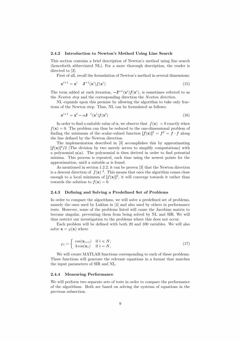
First of all, recall the formulation of Newton’s method in several dimensions:

xi+1 = xi � J�1(xi)f(xi) (15)

The term added at each iteration, �J�1(xi)f(xi), is sometimes referred to asthe Newton step and the corresponding direction the Newton direction.

NL expands upon this premise by allowing the algorithm to take only frac-tions of the Newton step. Thus, NL can be formulated as follows:

xi+1 = xi � �J�1(xi)f(xi) (16)

In order to find a suitable value of �, we observe that jf(x)j = 0 exactly whenf(x) = 0. The problem can thus be reduced to the one-dimensional problem offinding the minimum of the scalar-valued function jf(x)j2 = f2 = f � f alongthe line defined by the Newton direction.

The implementation described in [3] accomplishes this by approximatingjf(x)j2=2 (The division by two merely serves to simplify computations) witha polynomial p(�). The polynomial is then derived in order to find potentialminima. This process is repeated, each time using the newest points for theapproximation, until a suitable � is found.

As mentioned in section 1.2.2, it can be proven [3] that the Newton directionis a descent direction of jf(x)j2. This means that once the algorithm comes closeenough to a local minimum of jf(x)j2, it will converge towards it rather thantowards the solution to f(x) = 0.

2.4.3 Defining and Solving a Predefined Set of Problems

In order to compare the algorithms, we will solve a predefined set of problems,namely the ones used by Luksan in [4] and also used by others in performancetests. However, some of the problems listed will cause the Jacobian matrix tobecome singular, preventing them from being solved by NL and SIR. We willthus restrict our investigation to the problems where this does not occur.

Each problem will be defined with both 20 and 100 variables. We will alsosolve x = '(x) where

'i =�

cos(xi+1) if i < N ;3 cos(x1) if i = N:

(17)

We will create MATLAB functions corresponding to each of these problems.These functions will generate the relevant equations in a format that matchesthe input parameters of SIR and NL.

2.4.4 Measuring Performance

We will perform two separate sets of tests in order to compare the performanceof the algorithms. Both are based on solving the systems of equations in theprevious subsection.

9

In the first test, CPU time and number of subiterations will be measuredwhen the equations are solved using the initial guess given in the reports fromwhich they are taken. We will allow at most 100 iterations for the solution ofeach problem and if NL converges to a local minimum this will be noted.

In the second test, we will vary the initial guess and measure the numberof iterations required to solve the problems. Again, we will allow at most 100iterations and note if NL converges to a local minimum.

The first of these tests will determine the overall efficiency of the algorithms,while the second will determine their sensitivity to variations in the initial guess.

3 Realizing the Goals3.1 Implementing SIR and NL in MATLABOne thing that should be noted when writing in MATLAB is that it is optimizedfor the handling of vectors and matrices. One way in which this manifests itselfis that many operations will become more efficient if one can write them asmatrix or vector operations.

For instance, the following for loop:

for i = 1:Nx[i] = x[i]+5;

end

Can be more efficiently written as:

x = x+5

This often improves not only performance, but also clarity.

3.1.1 The Symbolic Toolbox

One major difference between Maple and MATLAB is that the latter does notnatively handle symbolic operations. This means, among other things, thatwhile it can approximate the Jacobian at any given point, it cannot nativelyderive it analytically and generate a formula. This is a notable drawback, asboth SIR and NL rely on Jacobian matrices.

It should be noted that MATLAB does handle symbolic variables via itssymbolic toolbox, which can be used to analytically compute Jacobians, amongother things. Depending on MATLAB version, this toolbox utilized either theMaple or the MuPad engine.

Unfortunately, using this toolbox turns out not to be feasible in practice, forreasons detailed below.

3.2 Efficiency Concerns when Using the Symbolic ToolboxAs mentioned in section 2.2, MATLAB has a built-in profiling tool, allowing usto study in detail how much time is spent executing each line of code.

Using this profiling tool we find that, for many problems, SIR spends morethan 95% of its execution time at the function subs, which substitute numericvalues into symbolic variables. The function subs, in turn, spends about half

10

its execution time converting symbolic expressions into character strings whichcan be passed as arguments to Maple.

Furthermore, the jacobian function spends about half its execution timeconverting the resulting Maple matrix into a symbolic matrix in MATLAB.

Thus, using the symbolic toolbox will lead to a significant amount of com-putational overhead, to the point that the overhead often amount to over 90%of the execution time!

The solution that was chosen for this problem was to define ' and its Ja-cobian as character strings, describing functions depending on x. By assigningx = p in the MATLAB environment and using the command eval, the functionvalue at the point p can be computed.

For instance: assume we wish to evaluate

'(x) =

24 cos(x2)

cos(x3)3 � cos(x1)

35

at the point

x =

24�2�2�2

35

This is accomplished with the following MATLAB code:

phi = ’[cos(x(2);cos(x(3));3*cos(x(1))]’;x = [-2;-2;-2];phi_x = eval(phi);

The Jacobian will be derived from ' by issuing a direct call to the Maplecore contained in the symbolic toolbox. All other dependencies upon Maple orthe symbolic toolbox is removed.

It should be noted that this solution is implemented in MATLAB 6.1. Itwill not work in recent versions of MATLAB, where the Maple core has beenreplaced with MuPad and may or may not work in intermediate versions.

A version that is more likely to work in current and future versions of MAT-LAB is based on the Maple toolbox (see section 3.4.1). Its source code can befound in appendix B.5.

3.2.1 Verifying the Implementation

In order to assure the correctness of the implementations, any roots found weretested against the condition f(x) = x.

Furthermore, the MATLAB and Maple implementations were compared.Due to differences in floating point roundoff, the convergence criterion that twosuccessive solutions should differ by only a small amount, may fail to hold afterthe exact same number of iterations. Thus, a small variation in the numberof iterations required to solve a particular problem is to be expected. Themeasured variations were deemed to be within reasonable margin.

11

3.3 Improving Efficiency of the AlgorithmThe efficiency of the algorithm (as opposed to the efficiency of the MATLABimplementation, as detailed above) was improved in several ways, detailed be-low:

3.3.1 Utilizing Sparse Matrix Structures

Sparsity is often utilized to improve efficiency when inverting matrices. This isbecause matrix inversion has a time complexity of N3 for a problem of size N ,which often dominates the theoretical time complexity of the algorithm.

However, in practical applications of SIR during the work on this thesis, thetime spent on Jacobian inversions was negligible. Since the Jacobian matricesoften need to be transformed into a more suitable form before the sparsity canbe exploited, this appears to be a wasted effort.

Conversely, Jacobian evaluations often dominate the execution time, andsparsity of the Jacobian matrix can be exploited in order to make these moreefficient, since only the non-zero elements need to be considered.

The same considerations are relevant in the computations of the A matrix,which requires multiplication with the diagonal matrix R�I (see section 1.2.2).

Since sparse definitions provide computational overhead, they are undesir-able for small or dense problems. It may also require more pre-processing togenerate a sparse Jacobian than a dense one.

To accommodate for this, SIR was implemented as callable with either denseor sparse definitions. However, the definition of R � I was set to sparse at alltimes, even though it slightly decreases performance for small problems. Therationale for this decision is that these small problems take relatively short timeto solve anyway.

3.3.2 Decreasing the Number of Quasi-Monotonicity Checks

Subiterating is a costly process: in order to maintain quasi-monotonicity, 'must be evaluated at a predetermined number of points between the currentguess and the next.

The default value of additional points, aside from the already known valueat the current guess, is 10. For this value, the additional function evaluationsoften dominate the execution time.

In the one-dimensional implementation of SIR, these evaluations are cru-cial for maintaining monotonicity. However, in the general case, monotonicitycannot be guaranteed by any means, making these computations less critical.

It should be noted, however, that for a global minimum to exist, it mustalso be a local minimum in each dimension. Thus it is still worthwhile to assurethat we do not overshoot these local minima as we encounter them.

In summary, it is desirable to reduce the amount of additional evaluations,while we do not wish to eliminate them altogether. Experiments indicate thatlowering the number of evaluations to a single additional point (for a total oftwo points) has little overall impact on convergence.

This also allows for implementation-specific optimizations since the valueof the governing parameter can now be hard coded. This can also potentiallyimprove the clarity of the code.

12

3.3.3 Using Subiterations as a Last Resort

Even with the above improvement, subiterations remain costly and, more impor-tantly, often unnecessary in practice. Indeed, they may even prove detrimentalto convergence.

For instance, when solving the problems listed in section 2.4.3, the algo-rithm always required more iterations when subiterations were used, sometimespreventing convergence within the allotted 100 iterations altogether. For otherproblems such as eq. 17, subiterations are crucial to finding a solution.

A good strategy, then, would be to attempt to find a solution without subit-erating, resorting to subiterations if none is found. To accommodate this usage,the algorithm will not use subiterations unless the user specifies this by passingan additional input argument.

3.3.4 Removal of Mirroring

Another crucial part of maintaining monotonicity in the one-dimensional caseis to mirror the iterating function if the solution is moving away from the root.In the general case, however, we cannot determine the directions of the root.We therefore resort to using the Newton step as a guideline, since it can beproven to be a descent direction [3]. Thus, much like was the case with themonotonicity checks discussed in section 3.3.2, this is less crucial in the generalcase.

Experiments indicate that, by removing the mirroring from the algorithm,convergence is made slightly more dependent on the value of the initial guess.However, the performance and clarity of code gained was decided to outweighthe negatives. Thus, mirroring is no longer part of the general algorithm.

3.3.5 Making Subiterations Conditional

Often when the algorithm fails to converge, it is because the solution starts torapidly shoot off in some direction. This suggests that subiterations are neededthe most when the step length is increasing faster than at a certain rate. Thisprocedure also safeguards against near-singular values of the elements of A.

Mathematically, we subiterate when jjx(i) � x(i�1)jj < c � jjx(i+1) � x(i)jj,where x(i) is the estimated root after the i:th iteration.

Experiments indicate that c = 1 is a suitable value, yielding fast and stableconvergence.

3.4 Incorporating SIR into GWRMThe incorporation of SIR into GWRM can be broken down into the followingsteps:

3.4.1 Interfacing MATLAB and Maple Using the Maple Toolbox

Not to be confused with MATLAB’s own symbolic toolbox, the Maple toolbox,developed by Maplesoft, is available to Maple users. It requires an installationof Maple to be present on the computer, which is why it is not feasible in thepure MATLAB implementation.

13

Unlike the symbolic toolbox, the Maple toolbox utilizes data structures thatcan store symbolic variables in such a way that they are readable from memoryby both Maple and MATLAB. Hence, the overhead caused by string manipula-tions mentioned in section 3.2 is removed.

It is now possible to define variables in the Maple environment, pass them toSIR in the MATLAB environment and make the results available in the Mapleenvironment.

3.4.2 Modifying the Source Code

The data structures that are readable in both programs, however, are not theones initially used in the Maple implementation of GWRM. Thus, minor changesmust be made to it.

Variables defined using the aforementioned structures become available inthe MATLAB environment by defining (MATLAB) symbolic variables with thesame name there.

Furthermore, the MATLAB implementation of SIR must be modified in twoways. The first is to replace the strings with symbolic variables. Secondly,in order to avoid working with very large Jacobian matrices, we partition thespatial dimension of the problem into subdomains and iterate over these sep-arately using an inner for loop. These essentially add another dimension toall vectors and matrices. MATLAB has a three-dimensional matrix data struc-ture, and matrices allow the engine to optimize performance. Thus, it makessense to use three-dimensional matrices for the Jacobian and A matrix and atwo-dimensional matrix for the function '.

In the original Maple implementation, the result was returned as a vectorwhose elements were the approximations of x after each iteration. Here, it willbe replaced by a cell array consisting of M cells. A cell array is essentially anarray which can have arbitrary (and dissimilar) data types as their elements.Here, the m:th cell will contain a matrix which in turn has columns containingthe solution after each iteration step.

The Maple toolbox allows Maple code to be executed from within MATLAB,but not vice versa. Thus, the following routine will be followed:

1. Execute Maple code defining the problem.

2. Define symbolic variables in MATLAB.

3. Call SIR, passing symbolic variables as arguments.

3.5 Comparison with Newton’s Method Using Line SearchSince the MATLAB implementation of SIR accepts function definitions as char-acter strings, this is the way we must define the problems to be solved.

MATLAB functions were created corresponding to each of the problemsdescribed in section 2.4.3, with input parameters allowing the user to specifythe problem size. The user is also able to decide whether the problem shouldbe defined as '(x) = 0, to be solved using NL, or as '(x) + x = x to be solvedusing SIR. The function then returns the appropriate ' as a character string.

14

3.5.1 Measuring CPU Time and Number of Iterations

The problems mentioned above were then solved in both 20 and 100 dimensions,using both SIR and NL.

It should be noted that this was done while running Microsoft Windows,so a small amount of background computation could not be avoided. However,to reduce the impact of the operating system running in the background, theproblems were solved 20 times, and the lowest execution time was tabulated.

In order to verify the above method, the test was repeated for some problemsand results proved consistent even if they were gathered at different times ordates.

Apart from execution time, the required number of iterations was also tab-ulated.

3.5.2 Measuring Sensitivity to Variations in Initial Guess

In this work, a new scheme for visualizing sensitivity to the initial guess hasbeen developed.

For each problem, a grid of 61�61 initial guesses was constructed. A surfaceplot defined by the function j'j2=2 was added to help identify behaviour nearlocal minima, since this is the function minimized by NL.

At each of the 61 � 61 grid points, the convergence characteristics of thealgorithm measured was represented with a color:

Red: no convergence within the allotted 100 iterations.

Orange: convergence to a local minimum (only relevant for NL).

Cyan: slow convergence.

Blue: fast convergence.

Note that red and orange are discrete values, while convergence is denoted bya color somewhere between cyan and blue depending on speed.

This scheme has the benefit of allowing both convergence characteristics andthe position of local minima to be accessible at a glance. However, in order forthis section to be possible, the problems must be solved in only two dimensions.Since not all problems were defined for two dimensions, this part was restrictedto those that were. A possible way to extend the idea to problems of largerdimensionality is discussed in section 5.3.

4 Results4.1 Translation of SIR into MATLAB, improved efficiency.Pseudo code for the improved version of the SIR algorithm, as well as MATLABsource code is found in appendix B.2. Source code for the helper functions usedcan be found in appendix B.6.

15

4.2 Incorporation of SIR into GWRM.The Source code is found in appendix B.3, which contains complete listingsof all files used to solve Burgers’ equations using the Maple/MATLAB hybridimplementation.

Timing both the pure Maple and Maple/MATLAB versions of the codeyielded the following execution times (rounded to whole seconds):

Pure Maple: 50 sec.MATLAB/Maple: 27 sec.

Note that the computer used is not the same as the one used when comparingSIR to NL, so comparisons between the two sets of measurements will not bevalid.

4.3 Comparison to NL.4.3.1 Implementation of NL in MATLAB.

Source code of the files specific to the MATLAB implementation of NL is foundin appendix B.4, while source code of any helper functions used can be locatedin appendix B.6

4.3.2 CPU Time and Iterations Required.

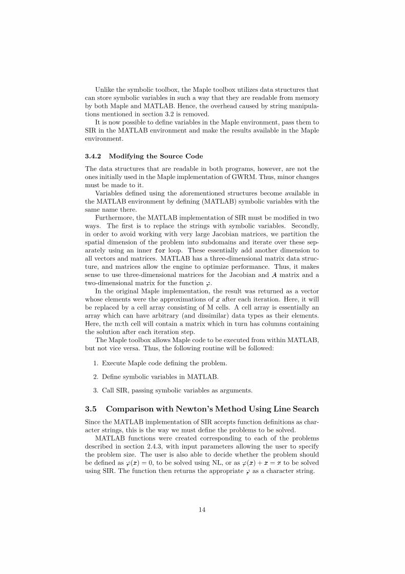
Table 1 lists number of iterations required and time taken when solving theproblems mentioned in section 2.4.3. This is done four times, once for eachcombination of problem size (N = 20 or N = 100) and algorithm used (NL orSIR).

In order to facilitate comparison between the four columns, sums and stan-dard deviations are computed for both time and number of iterations.

Note that, as mentioned in section 2.4.3, problems 5, 10 and 13 are ex-cluded, as MATLAB reported singular or near-singular Jacobian matrices forthese problems. This affected both SIR and NL.

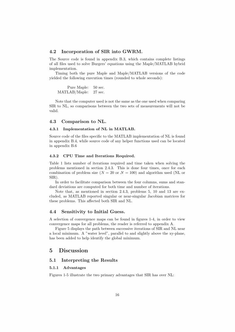
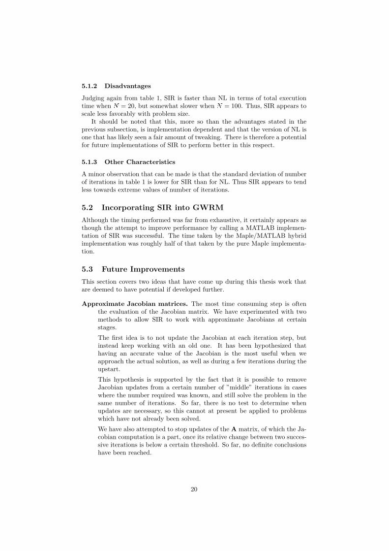
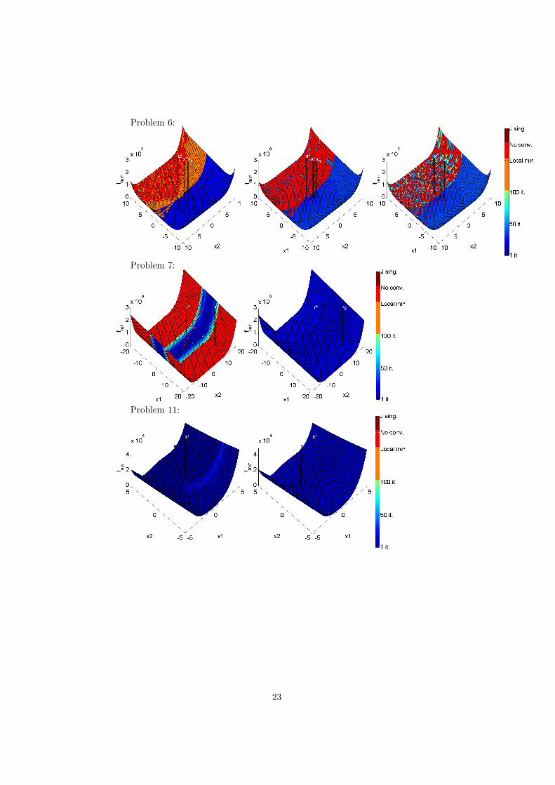
4.4 Sensitivity to Initial Guess.A selection of convergence maps can be found in figures 1-4, in order to viewconvergence maps for all problems, the reader is referred to appendix A.

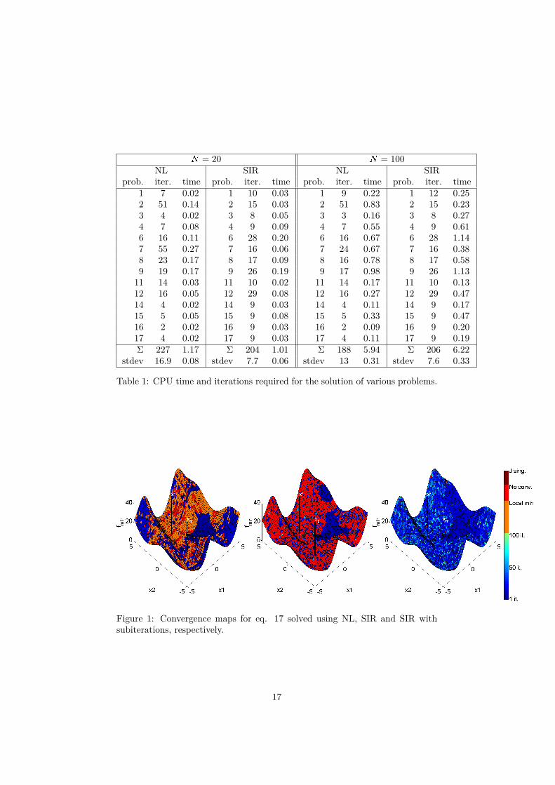
Figure 5 displays the path between successive iterations of SIR and NL neara local minimum. A ”water level”, parallel to and slightly above the xy-plane,has been added to help identify the global minimum.

5 Discussion5.1 Interpreting the Results5.1.1 Advantages

Figures 1-5 illustrate the two primary advantages that SIR has over NL:

16

N = 20 N = 100NL SIR NL SIR

prob. iter. time prob. iter. time prob. iter. time prob. iter. time1 7 0.02 1 10 0.03 1 9 0.22 1 12 0.252 51 0.14 2 15 0.03 2 51 0.83 2 15 0.233 4 0.02 3 8 0.05 3 3 0.16 3 8 0.274 7 0.08 4 9 0.09 4 7 0.55 4 9 0.616 16 0.11 6 28 0.20 6 16 0.67 6 28 1.147 55 0.27 7 16 0.06 7 24 0.67 7 16 0.388 23 0.17 8 17 0.09 8 16 0.78 8 17 0.589 19 0.17 9 26 0.19 9 17 0.98 9 26 1.13

11 14 0.03 11 10 0.02 11 14 0.17 11 10 0.1312 16 0.05 12 29 0.08 12 16 0.27 12 29 0.4714 4 0.02 14 9 0.03 14 4 0.11 14 9 0.1715 5 0.05 15 9 0.08 15 5 0.33 15 9 0.4716 2 0.02 16 9 0.03 16 2 0.09 16 9 0.2017 4 0.02 17 9 0.03 17 4 0.11 17 9 0.19Σ 227 1.17 Σ 204 1.01 Σ 188 5.94 Σ 206 6.22

stdev 16.9 0.08 stdev 7.7 0.06 stdev 13 0.31 stdev 7.6 0.33

Table 1: CPU time and iterations required for the solution of various problems.

Figure 1: Convergence maps for eq. 17 solved using NL, SIR and SIR withsubiterations, respectively.

17

Figure 2: Convergence maps for problem 7 solved using NL and SIR, respec-tively.

Figure 3: Convergence maps for problem 14 solved using NL and SIR, respec-tively.

Figure 4: Convergence maps for problem 17 solved using NL, SIR and SIR withsubiterations, respectively.

18

Figure 5: Convergence path when solving equation 17 with NL and SIR, respec-tively. ”Water level” added for clarity.

Reduced dependency on initial guess. From the convergence maps it isclear that SIR allows for convergence for a wider range of initial guessesfor the problems attempted.Some problems (4,7 and 14) converge nearly unconditionally in the illus-trated region when solved with SIR, whereas this is not the case for NL.Other problems (equation 17 and problem 17) have similar characteristicswhen solved with NL and SIR without subiterations, but converge atalmost every point in the region when subiterations are used.Problems that converge unconditionally in the region when solved withNL (11,15), do so also when solved with SIR.Only two of the problems tested, namely problems 2 and 6, retain theirhigh sensitivity to the initial guess for all three algorithms (NL, SIR andSIR using subiterations). Problem 2 also illustrates how subiterations cansometimes cause SIR to perform considerably worse.Thus, judging from the problems tested, SIR performs at least as well as,and often much better than, NL in this respect, especially if subiterationsare used.

Cannot get stuck in local minima. As noted in section 2.4.2, NL convergesto a minimum of fmin = jf(x)j2, even if this is a local minimum. Incontrast, SIR, like the original Newton’s method, doesn’t rely on fmin forconvergence, and thus cannot be fooled by its local minima. As mentionedpreviously, this behaviour is illustrated in fig 5.

19

5.1.2 Disadvantages

Judging again from table 1, SIR is faster than NL in terms of total executiontime when N = 20, but somewhat slower when N = 100. Thus, SIR appears toscale less favorably with problem size.

It should be noted that this, more so than the advantages stated in theprevious subsection, is implementation dependent and that the version of NL isone that has likely seen a fair amount of tweaking. There is therefore a potentialfor future implementations of SIR to perform better in this respect.

5.1.3 Other Characteristics

A minor observation that can be made is that the standard deviation of numberof iterations in table 1 is lower for SIR than for NL. Thus SIR appears to tendless towards extreme values of number of iterations.

5.2 Incorporating SIR into GWRMAlthough the timing performed was far from exhaustive, it certainly appears asthough the attempt to improve performance by calling a MATLAB implemen-tation of SIR was successful. The time taken by the Maple/MATLAB hybridimplementation was roughly half of that taken by the pure Maple implementa-tion.

5.3 Future ImprovementsThis section covers two ideas that have come up during this thesis work thatare deemed to have potential if developed further.

Approximate Jacobian matrices. The most time consuming step is oftenthe evaluation of the Jacobian matrix. We have experimented with twomethods to allow SIR to work with approximate Jacobians at certainstages.The first idea is to not update the Jacobian at each iteration step, butinstead keep working with an old one. It has been hypothesized thathaving an accurate value of the Jacobian is the most useful when weapproach the actual solution, as well as during a few iterations during theupstart.This hypothesis is supported by the fact that it is possible to removeJacobian updates from a certain number of ”middle” iterations in caseswhere the number required was known, and still solve the problem in thesame number of iterations. So far, there is no test to determine whenupdates are necessary, so this cannot at present be applied to problemswhich have not already been solved.We have also attempted to stop updates of the A matrix, of which the Ja-cobian computation is a part, once its relative change between two succes-sive iterations is below a certain threshold. So far, no definite conclusionshave been reached.

20

Convergence maps for N-dimensional problems. One possible way to ex-tend the concept of convergence maps to an arbitrary number of equationsis to choose two dimensions, perhaps randomly, to map.

AcknowledgementI would like to thank the people who helped me complete this thesis:

Jan Scheffel, my supervisor, for his encouragement, ideas and patient expla-nations.

Kjell Pernestal, for helping me shape this report out of the chaos that camebefore it.

Malin Drevin, for emotional and financial support.

References[1] J. Scheffel, TRITA-ALF-2004-03, Royal Institute of Technology, Stockholm,

Sweden, 2004.

[2] J. Scheffel, TRITA-EE-2006-006, Royal Institute of Technology, Stockholm,Sweden, 2006.

[3] W. H. Press, S. A. Teukolsky, W. T. Vetterling and B. P. Flannery, Numer-ical Recipes in C++ Second Edition, Cambridge University Press, 2002.

[4] L. Luksan, Inexact Trust Region Method for Large Sparse Systems of Non-linear Equations, Journal of Optimization Theory and Applications, Volume81, Issue 3 (1994).

21

AppendicesA Complete List of Convergence MapsAll maps are ordered, from left to right, by the algorithm used: NL, SIR andSIR with subiterations if used.

Eq. 17:

Problem 2:

Problem 4:

22

Problem 6:

Problem 7:

Problem 11:

23

Problem 14:

Problem 15:

Problem 16:

24

Problem 17:

B Source CodeThis section will list the source code used to run the implementations of SIR,NL and GWRM generated in this thesis. Helper functions used will be listedlast, but their intended purpose will be made clear in the sections where theyare used.

B.1 Sparse Jacobian DefinitionsBoth SIR and NL allow the user to define the Jacobian as either dense or sparse.

Since SIR and NL require functions to be represented as strings, it is notpossible to simply use the built-in MATLAB command sparse(J) to convert Jinto a sparse representation.

However, another built-in representation can be used in a slightly modifiedfashion: MATLAB allows us to represent a matrix, A, with the three vectors r,c and B. Here, B contains the non-zero elements of A while r and c contain theirrow and column indices, respectively. Thus the following holds:

A(r(i),c(i)) = B(i);

If we replace B with a string, we can allow it to contain functions which canbe passed to SIR or NL. For instance, the following, dense, Jacobian:

J = ’[0 -sin(x2) 0; 0 0 -sin(x3); -3*sin(x1) 0 0]’;

can be represented in the following, sparse, fashion:

r = [1,2,3];c = [2,3,1];J = ’[-sin(x2),-sin(x3),-3*sin(x1)]’

B.2 MATLAB Implementation of SIRThe pure MATLAB implementation of SIR is intended to be used in a fashionsimilar to the following:

25

% Define functionf = ’[cos(x2);cos(x3);3*cos(x1)]’;% Define initial guessx0 = [-2;-2;-2];% Compute JacobianJ = jac(f);% Find root, no subiterationsU = SIR(f,J,x0);

Here, jac is a helper function designed to compute the Jacobian of a functiondefined as a string, it is listed in appendix B.6.1.

Subiterations are activated by passing an additional boolean true whencalling SIR:

% Find root using subiterationsU = SIR(f,J,x0,true);

Furthermore, the jac function returns a sparse representation if called likethis:

% Compute sparse Jacobian[r,c,J] = jac(f);

This can then be passed to SIR by putting the r, c and J in a cell array, likethis:

% Find root, no subiterations, sparse JacobianU = SIR(f,{r,c,J},x0);

B.2.1 Pseudo Code for SIR

Input:

': A representation of the function ' : RN ! RN .

J : A representation of the Jacobian J'.

x0: An initial estimate for the root of x = '(x).

sub: A boolean variable indicating whether or not subiterations are to be used.

Output:

x�: The root of x = '(x).

Parameters:

N : Number of equations.

26

dΦ=dx0: Initial value of all @Φi=@xi.

Default values:0:9 when not subiterating.0:9999 when subiterating.

Rfac: Vector determining the rate at which @Φi=@xi is decreased at each iter-ation.

Default values:0:5 when not subiterating.0:8 when subiterating.

tol: Solution accuracy.

Default value: 10�8

Imax: Maximum number of iterations.

Default value: 100

Is: Maximum number of subiterations.

Default value: 1000 (This is intentionally set very high, since subitera-tions will still cease when certain conditions are met)

�max: Maximum allowed magnitude of A matrix elements.

Default value: 2

Mc: Parameter for monotonicity check.

Default value: �5 � 10�2

Functions:

A(R; J�1) = I + (R� I)J�1

Φ(x; ';A) = A(x� ') + '

Iteration loop:

% InitializeR := dΦ=dx0 � Ix(�1) := 0% Computations are to be carried out on Jf rather than J'Jf := I � Jfor i from 1 to Imax do

% Update Aphi(i�1) := '(x(i�1))J

(i�1)f := Jf (x(i�1))Jinv := inv(J (i�1)

f )A := A(R; Jinv)

% Compute new guess, xx(i) := Φ(x(i�1); phi(i�1); A)

27

% Subiterations beginif sub = true and max(jx(i) � x(i�1)j � jx(i�1) � x(i�2)j) > 0 then

for j from 1 to Is do% Compute Phi at current xphi(i) := '(x(i))Phi(i) := Φ(x(i); phi(i); A)

% Check validity of xfor n from 1 to N do

% Test for root between last and current guesstest1 := x(i�1) � x(i) � (x(i)

n � Phi(i)n ) < Mc

% Test for critically large Atest2 := 9m 2 [1; N ] : jAn;mj < �max

% Increase R if necessaryif test1 = true or test2 = true then

Rn;n := 3Rn;n+14

else% Exit subiterationsbreak

endifendfor

% Update A and xA := A(R; Jinv)x(i) := Φ(x(i�1); phi(i�1); A)

endforendif% Subiterations end

% Test for convergenceif mean(jx(i) � x(i�1)j) < tol then break

% Decrease RR := Rfac �R

endforreturn x(n)

B.2.2 SIR.m

Here, we return not only the final solution, but a matrix containing the solutionafter each iterations step.

It should also be noted that the algorithm uses the helper function addPar,listed in B.6.4, to replace every occurrence of, for instance x10 with x(10). Thisallows the command eval to properly insert the tenth element of the vector x.The reason that the string aren’t defined like this in the first place is that thejac function, listed in B.6.1, needs to construct symbolic variables with namesidentical to the elements of x, and parentheses are not allowed in variable names.

28

function U = SIR(fstr,Jstr,x0,sub)% U = SIR(fstr,Jstr,x0)% Solves the problem f(x) = x without using subiterations.%% fstr is a string containing the function definition for f%% Jstr has either of the following forms:% - dense representation: Jstr is a string containing the% function definition of the matrix J% - sparse representation: Jstr = {r,c,Jsp} where r contains% row indices, c contains column indices and Jsp is a string% representation of the vector containing the non-zero% elements of J.%% x0 is the initial guess.%%% U = SIR(fstr,Jstr,x0,true)% Solves the problem f(x) = x using subiterations.% fstr, Jstr and x0 as above.

%%%%%%%%%%%%%%%%%% Parameters %%%%%%%%%%%%%%%%%%if nargin < 4

sub = 0; % Default to no subiterationsendif sub

% Values when subiteratingRfac=0.8; % Reduction of R at each iterationdPdx=0.9999; % Initial values of R

else% Values when notRfac=0.5; % Reduction of R at each iterationdPdx=0.9; % Initial values of R

end

N=length(x0); % Number of equationstol=1e-8; % Solution accuracyimax=100; % Maximum number of iterationsJs=1000; % Maximum number of subiterationsa_c=2; % Critical magnitude for alphaS1_min=-5e-2; % Parameter for monotonicity check

%%%%%%%%%%%%%%%%%%%%%% Initialization %%%%%%%%%%%%%%%%%%%%%%

xold = zeros(size(x0)); % Store the old x0R = dPdx*ones(N,1); % R0U = []; % Solution matrix

% If Jstr is a cell, we extract its component partsif iscell(Jstr)

r = Jstr{1};c = Jstr{2};Jstr = Jstr{3};sparse_def = true;

elsesparse_def = false;

end

29

% replace every occurrence of ’xi’ with ’x(i)’Jstr = addPar(Jstr,N);fstr = addPar(fstr,N);

%%%%%%%%%%%%%%%%%%%%%% Iteration Loop %%%%%%%%%%%%%%%%%%%%%%for n = 1:imax

% Append current guess to UU = [U x0];

% --------------------% I: Compute new alpha% --------------------% Since fstr has x as its variable name, we assign x = x0 in order% to compute f(x0) and J(x0)x = x0;phi0 = eval(fstr);

J = eval(Jstr);% Transform J into I-Jif sparse_def

% Sparse versionJ = sparse(r,c,J,N,N);J = speye(N)-J;

else% Dense versionJ = eye(N)-J;

end% Test for singularityif issparse(J)

condJ = rcond(full(J));else

condJ = rcond(J);endif condJ == 0

warning(’Jacobian singular in SIR’);return;

end% Invert jacobianinvJ = inv(J);

% Compute R-IRI = RI_proc(R,N);% Compute alphaalpha = alpha_proc(RI,invJ,N);

% -----------------% II: Compute x1% -----------------x1 = Phi_proc(x0,phi0,alpha);

%%%%%%%%%%%%%%%%%%%%% Subiterations %%%%%%%%%%%%%%%%%%%%%% Only subiterate if step length is increasingif sub && max(abs(x1-x0) - abs(x0-xold)) > 0

% Precompute x0-Phi(x0) = x0-x1mon = x0-x1;

30

% -------------------------% III: Check validity of x1% -------------------------for m=1:Js

% Evaluate phi(x1)x = x1;phi1 = eval(fstr);

% - The element-wise multiplication means that each element% n of S1 is negative only if ,in the n:th dimension,% phi has opposite signs at x0 and x1.S1 = mon .* (x1-Phi_proc(x1,phi1,alpha));

% Check for critically large alpha by taking the row-wise maxS2 = max(abs(alpha),[],2);

% Perform all comparisons at once, store in boolean vector ifR% A particular row of ifR will be true if subiteration is% required in that dimension.ifR = (S2 >= a_c | S1 < S1_min);

% Break if no subiterations are neededif max(ifR) == 0

break;end

% Increase R towards Ifor i=1:N

% If subiterations are required in the i:th dimension,% increase the i:th row of Rif ifR(i) == 1

R(i) = (3*R(i)+1)*0.25;end

end% Update RIRI = RI_proc(R,N);

% Recompute alphaalpha = alpha_proc(RI,invJ,N);x1 = Phi_proc(x0,phi0,alpha);

end%% -----------------------%% Subiterations end here:%% -----------------------

end

% ------------------------% Accuracy test and update% ------------------------eps = mean(abs(x1-x0));

xold = x0; % Backup x0 so that it can be used to compare step lengths.x0 = x1;if eps < tol

breakend

% Decrease RR = Rfac*R;

end% Append final guess to UU = [U x0];

31

%%%%%%%%%%%%%%%%% Functions %%%%%%%%%%%%%%%%%function alpha = alpha_proc(RI,invJ,N)% Compute alpha = I + (R-I)*J^(-1)alpha = eye(N)+RI*invJ;

function Phi = Phi_proc(x,phi,alpha)% Computes Phi = alpha*(x-phi)+phi% x and phi are allowed to be matrices, in which case Phi will be alsoPhi = alpha*(x-phi)+phi;

function RI = RI_proc(Rd,N)% Computes R-I% Rd is a vector containing the diagonal elements of RRI = spalloc(N,N,N);for i=1:N

RI(i,i) = Rd(i)-1;end

B.3 MATLAB/Maple Hybrid Implementation of GWRMThis implementation consists of three parts:

Burger.mpl: Maple code defining all input arguments necessary to solve Burg-ers’ equations using GWRM.

SIR.m: A MATLAB implementation of SIR, modified to handle spatial sub-domains.

GWRM.m: MATLAB code tying the two together.

B.3.1 GWRM.m% Restart maple enginemaple(’restart’);

% Define problem in Mapleprocread(’Burger.mpl’);

% Extract symbolic variablesclear phi X Ns J;syms phi X Ns J;

% Convert X to doubleX = double(X);

% Call SIRU = SIR(phi,copy(J),X,0);

B.3.2 Burger.mpl

This is a largely unmodified version of the GWRM code for solving Burger’sequations given in [1]. Minor changes has been made near the end to use theMatrix and Array data structures.

32

Digits:=14:with(linalg):with(numapprox):with(orthopoly):

# Parameters.Ns:=2: #Number of spatial subdomainsm_max:=6: #Order of temporal modesn_max:=8: #Order of spatial modeskappa:=0.01: #Viscosity

# Subdomain stuff.Lt:=0: Rt:=5.0:

for j from 0 to Ns+1 doRx[j]:=evalf(j/(Ns+1)):xb[j]:=Rx[j]:Lx[j]:=Rx[j-1]:epsBC[j]:=0.0:od:

for j from 0 to Ns+1 doxb[j]:=Rx[j]:Lx[j]:=Rx[j-1]:epsBC[j]:=0.0:od:

BMAt:=0.5*(Rt-Lt):BPAt:=0.5*(Rt+Lt):for j from 1 to Ns doBMAx[j]:=0.5*(Rx[j+1]-Rx[j-1]):BPAx[j]:=0.5*(Rx[j+1]+Rx[j-1]):od:

# Support functions to Chebyshev expansions.for j from 1 to 2*max(m_max,n_max) do fp[j]:=1 od:fp[0]:=1/2:for k from -2*max(m_max,n_max) to 2*max(m_max,n_max) do delta[k]:=0 od:delta[0]:=1:

# The Chebyshev expansion.for j from 1 to Ns dotest_u[j]:=simplify(sum(sum(u[j][m,n]*fp[m]*fp[n]*T(m,(t-BPAt)/BMAt)*T(n,(x-BPAx[j])/BMAx[j]),m=0..m_max),n=0..n_max)):od:

# Procedures for computation of PWRM-coefficients for Burger’s equation.Derivative_2x:=proc(a,BMA,A)local Asum,k,m,M,n,N;global m_max,n_max;N:=n_max-1; #Derivatan minskar ordningen.for m from 0 to m_max doA[m,N+1]:=0;A[m,N+2]:=0;

for n from N+1 by -1 to 1 doA[m,n-1]:=A[m,n+1]+2*n*a[m,n]/BMA;od;

od;end:

33

Product_2D:=proc(A,B,C,K,L)local k,l,m,n,r,s,Ax,Bx;global delta,fp;

for k from 0 to 3*K dofor l from 0 to 3*L doAx[k,l]:=0;Bx[k,l]:=0; od: od:

for k from 0 to K dofor l from 0 to L doAx[k,l]:=fp[k]*fp[l]*A[k,l];Bx[k,l]:=fp[k]*fp[l]*B[k,l];od: od:

for r from 0 to 1*K dofor s from 0 to 1*L do

C[r,s]:=(1/4)*add(add(Ax[m,n]*((1+delta[r-m])*(1+delta[s-n])*Bx[abs(r-m),abs(s-n)]+(1+delta[r-m])*(1-delta[s])* Bx[abs(r-m),s+n]+(1-delta[r])* (1+delta[s-n])*Bx[r+m,abs(s-n)]+(1-delta[r])* (1-delta[s])* Bx[r+m,s+n])

,m=0..K),n=0..L);

od: od:

for k from 0 to 1*K do C[k,0]:=2*C[k,0] od:for l from 0 to 1*L do C[0,l]:=2*C[0,l] od:end:

Integral_2t:=proc(a,BMA,A)local Asum,m,n;global m_max,n_max;for n from 0 to n_max doAsum:=0:a[m_max+1,n]:=0:a[m_max+2,n]:=0:for m from 1 to m_max+1 doA[m,n]:=BMA*(a[m-1,n]-a[m+1,n])/(2*m);Asum:=Asum+cos(m*Pi)*A[m,n];od;A[0,n]:=-2*Asum;od;end:

# The PDE is transformed to Chebyshev space# and distributed into subdomains.for Is from 1 to Ns do

Derivative_2x(a, BMAx[Is],a1):Derivative_2x(a1,BMAx[Is],a2):Product_2D(a,a1,a3,m_max,n_max):for m from 0 to m_max dofor n from 0 to n_max doa4[m,n]:=-a3[m,n]+kappa*a2[m,n];od: od:Integral_2t(a4,BMAt,A0):assign(a,u[Is]):

34

for m from 0 to m_max dofor n from 0 to n_max doA[Is][m,n]:=A0[m,n]:od: od:unassign(’a’):

od:

# BC’s are applied.BC_proc:=proc(u)# BC:s are imposed at modal points n_max-1 and n_max.local ii,j,jx,k,mx,m,n,BCtest,del,Sol,S,Sd,i_Eq,Eq:

unassign(’u’):

for m from 0 to m_max doif Ns >= 2 thenS[1,0]:=sum(fp[q]*u[1][m,q]*T(q,(xb[0] -BPAx[1])/BMAx[1]),q=0..n_max):S[1,1]:=sum(fp[q]*u[1][m,q]*T(q,(xb[1]+epsBC[2]-BPAx[1])/BMAx[1]),q=0..n_max):S[1,2]:=sum(fp[q]*u[1][m,q]*T(q,(xb[2]-epsBC[1]-BPAx[1])/BMAx[1]),q=0..n_max):

for n from 2 to Ns-1 doS[n,0]:=sum(fp[q]*u[n][m,q]*T(q,(xb[n-1]+epsBC[n] -BPAx[n])/BMAx[n]),q=0..n_max):S[n,1]:=sum(fp[q]*u[n][m,q]*T(q,(xb[n] -epsBC[n-1]-BPAx[n])/BMAx[n]),q=0..n_max):S[n,2]:=sum(fp[q]*u[n][m,q]*T(q,(xb[n] +epsBC[n+1]-BPAx[n])/BMAx[n]),q=0..n_max):S[n,3]:=sum(fp[q]*u[n][m,q]*T(q,(xb[n+1]-epsBC[n] -BPAx[n])/BMAx[n]),q=0..n_max):od:

S[Ns,0]:=sum(fp[q]*u[Ns][m,q]*T(q,(xb[Ns-1]+epsBC[Ns] -BPAx[Ns])/BMAx[Ns]),q=0..n_max):S[Ns,1]:=sum(fp[q]*u[Ns][m,q]*T(q,(xb[Ns] -epsBC[Ns-1]-BPAx[Ns])/BMAx[Ns]),q=0..n_max):S[Ns,2]:=sum(fp[q]*u[Ns][m,q]*T(q,(xb[Ns+1] -BPAx[Ns])/BMAx[Ns]),q=0..n_max):fi:

if Ns = 1 thenS[1,0]:=sum(fp[q]*u[1][m,q]*T(q,(xb[0]-BPAx[1])/BMAx[1]),q=0..n_max):S[1,2]:=sum(fp[q]*u[1][m,q]*T(q,(xb[2]-BPAx[1])/BMAx[1]),q=0..n_max):Eq[1]:=subs(u=ux,S[1,0]):Eq[2]:=subs(u=ux,S[1,2]):fi:

if Ns = 2 thenEq[1]:=subs(u=ux,S[1,0]):Eq[2]:=subs(u=ux,S[1,2])-S[2,1]:Eq[3]:=subs(u=ux,S[2,0])-S[1,1]:Eq[4]:=subs(u=ux,S[2,2]):fi:

if Ns >= 3 thenEq[1]:=subs(u=ux,S[1,0]):Eq[2]:=subs(u=ux,S[1,2])-S[2,1]:for n from 2 to Ns-1 doEq[2*n-1]:=subs(u=ux,S[n,0])-S[n-1,1]:Eq[2*n] :=subs(u=ux,S[n,3])-S[n+1,1]:od:Eq[2*Ns-1]:=subs(u=ux,S[Ns,0])-S[Ns-1,2]:Eq[2*Ns] :=subs(u=ux,S[Ns,2]):fi:

35

for n from 1 to Ns doSol[n]:=solve({seq(Eq[ii],ii=2*n-1..2*n)},{seq(ux[n][m,j],j=n_max-1..n_max)});assign(Sol[n]):od:od:

end:

# Initial conditions (IC) are determined.# Here we use u(0,x) = x(1-x).# Note, that the coeffs are different for different intervals.for Is from 1 to Ns dofor n from 0 to n_max dob_IC[Is][n]:=0:od: od:

for j from 1 to Ns dob_IC[j][0]:=-2.*BPAx[j]^2+2.*BPAx[j]-1.*BMAx[j]^2:b_IC[j][1]:=-2.*BMAx[j]*BPAx[j]+BMAx[j]:b_IC[j][2]:=-.5000000000*BMAx[j]^2:od:

# All Chebyshev coefficients for the TP-WRM iterations are computed, # including BC and IC.for Is from 1 to Ns dofor n from 0 to n_max-2 do

for m from 0 to m_max doq[Is][m,n]:=A[Is][m,n]:

od:q[Is][0,n]:=q[Is][0,n]+2*b_IC[Is][n]:

od: od:

# TP-WRM coefficient equations are transformed to SIR equations.# First, the matrix a (dimension (m_max+1) X (n_max+1)) is turned into the vector x (length (m_max+1)

# Number of equations to be solved.N:=(m_max+1)*(n_max+1);

# Create the Matrix and Array (note the capitals) data structures to be used in MATLAB:X := Matrix(N,Ns):phi := Matrix(N,Ns):J := Array(1..N,1..N,1..Ns):BC_proc(u):

for Is from 1 to Ns dofor n from n_max-1 to n_max dofor m from 0 to m_max doq[Is][m,n]:=subs(ux=u,ux[Is][m,n]):od: od: od:

for Is from 1 to Ns dofor k from 1 to m_max+1 dofor j from 1 to n_max+1-0*2 dou[Is][k-1,j-1]:=x[(n_max+1)*(k-1)+j,Is]:od: od: od:

# Create phifor Is from 1 to Ns dofor k from 1 to m_max+1 dofor j from 1 to n_max+1 dophi[(n_max+1)*(k-1)+j, Is]:=expand(q[Is][k-1,j-1]):od: od: od:

36

# Create Jacobiansfor Is from 1 to Ns dofor j from 1 to N dofor k from 1 to N doJ[j,k,Is]:=diff(phi[j,Is],x[k,Is]):od:od:od:

% Create x0for Is from 1 to Ns dofor j from 1 to n_max+1 doX[j,Is]:=2.0*b_IC[Is][j-1]od: od:

B.3.3 SIR.m

There are a few ways in which this implementation differs from the pure MAT-LAB implementation listed in appendix B.2.2:

� An inner loop over spatial subdomains has been added.

� As mentioned in section 3.4.2, another dimension is added to matrices andvectors.

� ' and J are given as symbolic expressions rather as character strings.These symbolic expressions are evaluated as follows: First, a value is as-signed to the dependent variable, x, in the Maple environment using thesetmaple command. Then the expression is converted to a numeric rep-resentation using the double command.

� Since J is now a symbolic expression, it can be transformed into I � Jonce ,in the initialization step. In the pure MATLAB implementation,this was done after J was evaluated at each iteration loop.

function U = SIR(phi,J,x0,sub)% U = SIR(phi,J,x,x0)% Solves the problem phi(x) = x, with starting guess x0 without using% subiterations.%% phi is a symbolic NxM matrix, with M being the number of% spatial subdomains.%% x0 is a constant NxM matrix.%% J is a 3D NxNxM matrix, where the m:th slice contains% the NxN Jacobian of the m:th column of f with respect to the m:th column% of x%% U is a cell array consisting of M cells, The m:th cell contains a matrix% with columns containing the solution after each iteration step.%% U = SIR(phi_func,J_func,x0,sub)% As above, with the value of sub (true or false) determining whether or% not to use subiterations.

37


sub = false; % Default to no subiterationsendif sub



end

[N M] = size(x0); % Number of equationstol=1e-8; % Solution accuracyimax=100; % Maximum number of iterationsJs=1000; % Maximum number of subiterationsa_c=2; % Critical magnitude for alphaS1_min=-5e-2; % Parameter for monotonicity check

%%%%%%%%%%%%%%%%%%%%%% Initialization %%%%%%%%%%%%%%%%%%%%%%

xold = zeros(size(x0)); % Store the old x0R = dPdx*ones(N,M); % R0, now also an NxM matrixeps_acc = 1; % Dummy value for accuracy testx1 = x0; % x1 will be updated one spatial subdomain at a timefor i = 1:M

U{i} = []; % Initialize solution arrayend

% Transform J into I-Jfor i=1:M

if issparse(J(:,:,i))% Sparse versionJ(:,:,i) = speye(N)-J(:,:,i);

else% Dense versionJ(:,:,i) = eye(N)-J(:,:,i);

endendIJ = J;


% Inner loop over spatial subdomainsfor m = 1:M

% Update UU{m} = [U{m} x0(:,m)];

% --------------------% I: Compute new alpha% --------------------% Evaluate functions at x=x0setmaple(’x’,x0);

38

% Evaluate phi(x0) and IJ(x0)% Note that all xs and x0s may be present in each subdomainphi0 = double(phi(:,m));IJ0 = double(IJ(:,:,m));% Invert JacobianinvIJ = inv(IJ0);

% Compute R-I, here we need to use the m:th column of RRI = RI_proc(R(:,m),N);% Compute alphaalpha = alpha_proc(RI,invIJ,N);

% --------------% II: Compute x1% --------------% Update the m:th subdomain of x1x1(:,m) = Phi_proc(x0(:,m),phi0,alpha);

%%%%%%%%%%%%%%%%%%%%% Subiterations %%%%%%%%%%%%%%%%%%%%%% Only subiterate if step length is increasing in this subdomainif sub && max(abs(x1(:,m)-x0(:,m)) - abs(x0(:,m)-xold(:,m))) > 0

% Precompute x0-Phi(x0) = x0-x1 in this subdomainmon = x0(:,m)-x1(:,m);

% -------------------------% III: Check validity of x1% -------------------------for j=1:Js

% Evaluate functions at x=x1setmaple(’x’,x1);% Evaluate phi(x1)phi1 = double(phi(:,m));

% - The element-wise multiplication means that each element% n of S1 is negative only if ,in the n:th dimension,% phi has opposite signs at x0 and x1.S1 = mon .* (x1(:,m)-Phi_proc(x1(:,m),phi1,alpha));

% Check for critically large alpha by taking the row-wise maxS2 = max(abs(alpha),[],2); % Check for critically large alpha



break;end

% Increase the m:th column of R towards Ifor i=1:N

% If subiterations are required in the i:th dimension,% increase the i:th row of Rif ifR(i) == 1

R(i,m) = (3*R(i,m)+1)*0.25;end

end

39

% Update RIRI = RI_proc(R(:,m),N);

% Recompute alphaalpha = alpha_proc(RI,invIJ,N);x1(:,m) = Phi_proc(x0(:,m),phi0,alpha);

end% -----------------------% Subiterations end here:% -----------------------

end

% ------------------------% Accuracy test and update% ------------------------% compute accuracy in each subdomain, note that% eps_acc is NOT a cell, but a vector of size Meps_acc(m) = mean(abs(x1(:,m)-x0(:,m)));

xold(:,m) = x0(:,m); % Backup x0 so that it can be used to% compare step lengths.

x0(:,m) = x1(:,m);

% Decrease RR(:,m) = Rfac*R(:,m);

endif max(eps_acc) < tol

breakend

end% Add last point to Ufor m = 1:M

U{m} = [U{m} x0(:,m)];end

%%%%%%%%%%%%%%%%% Functions %%%%%%%%%%%%%%%%%function alpha = alpha_proc(RI,invJ,N)% Compute alpha = I + (R-I)*J^(-1)alpha = eye(N)+RI*invJ;

function Phi = Phi_proc(x,phi,alpha)% Computes Phi = alpha*(x-phi)+phi% x and phi are allowed to be matrices, in which case Phi will be alsoPhi = alpha*(x-phi)+phi;

function RI = RI_proc(Rd,N)% Computes R-I% Rd is a vector containing the diagonal elements of RRI = spalloc(N,N,N);for i=1:N

RI(i,i) = Rd(i)-1;end

B.4 MATLAB Implementation of NLFor a thorough description of this algorithm, the reader is directed to [3], whichcovers the C++ version this is adapted from.

The translation is in many ways similar to the translation of SIR from Mapleto MATLAB. For instance, functions are implemented as strings and evaluated

40

in the same fashion and for loops have been vectorized. A proper Jacobian hasalso replaced the finite difference approximations used in the C++ implemen-tation.

The implementation consists of two files, NL.m and lnsrch.m.

B.4.1 NL.mfunction U = newtNR(fstr,Jstr,x)% [U, check] = newtNR(fstr,Jstr,x0)%% Solve f(x) = 0, using Newton’s Method with Line Search.%% - x0 is the initial guess.% - fstr and Jstr are string representations of f and its% Jacobian, respectively.%% - check stores whether or not a spurious root (i.e. local% minimum) was encountered.

MAXITS = 100; % Maximum number of iterationsTOLF=1e-8; % Convergence criterion on function valuesTOLMIN=1e-12; % Criterion for spurious rootsSTPMX=100; % Scaled maximum step length in line searchesTOLX=1e-8; % Convergence criterion on x

% If Jstr is a cell, we extract its component partsif iscell(Jstr)

r = Jstr{1};c = Jstr{2};Jstr = Jstr{3};J_sparse = true;

elseJ_sparse = false;

end);

U = x; % Initialize solution matrixn = length(x); % Derive N from the length of x

% replace every occurrence of xi with x(i)Jstr = addPar(Jstr,n);fstr = addPar(fstr,n);

% compute f(x)fvec = eval(fstr);% compute fmin, the function to be minimizedf = fmin_func(fvec);

% Test for initial guess being a root.% Use more stringent test than simply TOLFif max(abs(fvec)) < 0.01*TOLF

check = false;return;

end% Calculate stpmax for line searchesstpmax = STPMX*max(norm(x),n);% Start of iteration loopfor its=1:MAXITS

% Compute jacobian at xfjac = eval(Jstr);if J_sparse

41

fjac = sparse(r,c,fjac,n,n);end% Test for singularityif J_sparse

condJ = rcond(full(fjac));else

condJ = rcond(fjac);endif condJ == 0

warning(’Jacobian singular in newtNR’);check = false;return

end% Compute the gradient of f for the line search% NOTE: for column vectors, the jacobian vector needs to be transposedg = fjac’*fvec;xold = x; % Store x,fold = f; % and f% Compute Newton stepp = -inv(fjac)*fvec;% Perform line search[x,f,fvec,check] = lnsrch(xold,fold,g,p,stpmax,fstr,@fmin_func);

% Append guess to solutionU = [U x];

% Test for convergence on function valuesif max(abs(fvec)) < TOLF

check = false;return;

end% Check for gradient of f zero, i.e. spurious convergence.if check

den = max(f,0.5*n);test = max(abs(g).*max(abs(x),1)/den);check = (test < TOLMIN);return;

end% Test for convergence on xif max(abs(x-xold)./max(abs(x),1)) < TOLX

return;end

enderror(’MAXITS exceeded in newtNR’);

% The function of which to find a global minimum: <f,f>/2function fmin = fmin_func(fvec)fmin = 0.5*dot(fvec,fvec);

B.4.2 lnsrch.mfunction [x1, f1, fvec1, check] = lnsrch(x0, f0, grad, dx, stpmax, fstr, fmin)% The heart of the line search function from numerical recipes

alpha = 1e-4; % Ensures sufficient decrease in function valuetolx = eps; % Convergence criterion on xlambda2 = 0;f2 = 0;

check = false;

42

% Scale if attempted step is too bigif norm(dx) > stpmax

dx = dx .* stpmax/norm(dx);endslope = dot(grad,dx);if slope >= 0

error(’Roundoff problem in lnsrch’);end% Compute lambda_mintest = max(abs(dx)./max(abs(x0),1));lambda_min = tolx/test;% Always try the full Newton step firstlambda = 1;% Start of iteration loopwhile true

x1 = x0 + lambda*dx;x = x1;fvec1 = eval(fstr);f1 = feval(fmin,fvec1);

% Convergence on x. For zero finding,% the calling program should verify the convergenceif lambda < lambda_min

x1 = x0;check = true;return;

% Sufficient function decrease (first Wolfe cond.)elseif f1 < f0 + alpha*lambda*slope

return;% Backtrackelse

% First timeif lambda == 1

tmplam = -slope/(2*(f1-f0-slope));% Subsequent backtrackselse

rhs1 = f1-f0-lambda*slope;rhs2 = f2-f0-lambda2*slope;X(1) = (rhs1/(lambda*lambda) - rhs2/(lambda2*lambda2))/(lambda-lambda2);X(2) = (-lambda2*rhs1/(lambda*lambda)+lambda*rhs2/(lambda2*lambda2))/(lambda-lambda2);

% Update alpha% A = 0if(X(1) == 0)

tmplam = -slope/(2*X(2));% A != 0else

disc = X(2)*X(2) - 3*X(1)*slope;if (disc < 0)

% Imaginary roots, set lambda = 0.5*lambda1tmplam = 0.5*lambda;

elseif X(2) <= 0tmplam = (-X(2) + sqrt(disc))/(3*X(1));

elsetmplam = -slope/(X(2) + sqrt(disc));

endend

end% lambda <= 0.5*lambda1if tmplam > 0.5*lambda

tmplam = 0.5*lambda;end

43

endlambda2 = lambda;f2 = f1;% lambda >= 0.1*lambda1lambda = max(tmplam,0.1*lambda);

end

B.5 MATLAB/Maple Hybrid Implementation of SIRIn the pure MATLAB implementation of SIR, limitations of the symbolic tool-box were circumvented using methods that are only viable in specific (older)versions of MATLAB. For readers who wish to implement SIR in a more re-cent version, we present a version utilising the Maple toolbox, as mentioned insection 3.4.1.

This implementation will have many similarities to the implementation ofGWRM given in appendix B.3. It consists of the following parts:

prob ¡x¿.mpl: Maple code defining ' and the initial guess x0.

jac.mpl: Maple code computing the Jacobian of '.

jac sp.mpl: Maple code computing the Jacobian of ' and storing it as a sparsedefinition (see appendix B.1).

SIR.m: A MATLAB implementation of SIR.

runSIR.m: MATLAB code tying the above together.

B.5.1 runSIR.m

When executed in MATLAB, runSIR.m will solve the problem specified in itsparameters and store the result in the matrix U.

Note that we set the value of N in the Maple environment, so that it can beused in the function definitions and Jacobian computations.

% Parametersprob = ’prob_cos’; % Which problem to solvesparse_def = true; % Whether or not to define jacobian as sparsesub = true; % Whether or not to subiterateN = 2; % Number of dimensions

% Restart Maple enginemaple(’restart’);setmaple(’N’,N);

% Define problem% Run the specified problem definitionprocread([prob ’.mpl’]);

% Compute jacobianif sparse_def

% Sparse definitionprocread(’jac_sp.mpl’);

else% Dense definitionprocread(’jac.mpl’);

end

44

% Extract symbolic variablesclear phi J x0 r c;syms phi J x0;if sparse_def

syms r c; % Extract additional variables requiredJ = {r,c,J}; % Store entire jacobian definition in cell

end

% Execute SIRU = SIR(phi,J,x0,sub);

B.5.2 prob cos.mpl

This is an example of how a problem definition can be implemented, which willdefine the problem given in eq. 17. It is important that the variables are namedphi and x0, since these names will be referenced later on.

As was the case in appendix B.3, we use the Matrix data structure, makingvariables available in both the Maple and MATLAB environments.

x0 := Matrix(N,1):phi := Matrix(N,1):for j from 1 to N-1 do

phi[j] := cos(x[j+1,1]):od:phi[N] := 3*cos(x[1,1]):for j from 1 to N do

x0[j] := -2:od:

B.5.3 jac.mpl

Here we compute the Jacobian of the function stored in phi with respect to xand store the result in the Matrix J.

J := Matrix(N,N):for j from 1 to N do

for k from 1 to N doJ[j,k] := diff(phi[j,1],x[k,1]):

od:od:

B.5.4 jac sp.mpl

This time, we store only the nonzero elements of the Jacobian in the Array J,and their column and row indices in the Arrays r and c, respectively.

# Define Arrays that are sure to fit the at most# N*N nonzero elementsJ := Array(1..N*N):r := Array(1..N*N):c := Array(1..N*N):# Counter for nonzero elementscount := 0:for j from 1 to N do

for k from 1 to N do# Test if derivative is nonzerod := diff(phi[j,1],x[k,1]):

45

if d <> 0 then# Increase countercount := count + 1:# Store indicesr[count] := j:c[count] := k:# Store the current derivativeJ[count] := d:

fi:od:

od:# Shrink the arrays to fit the dataJ := J[1..count]:r := r[1..count]:c := c[1..count]:

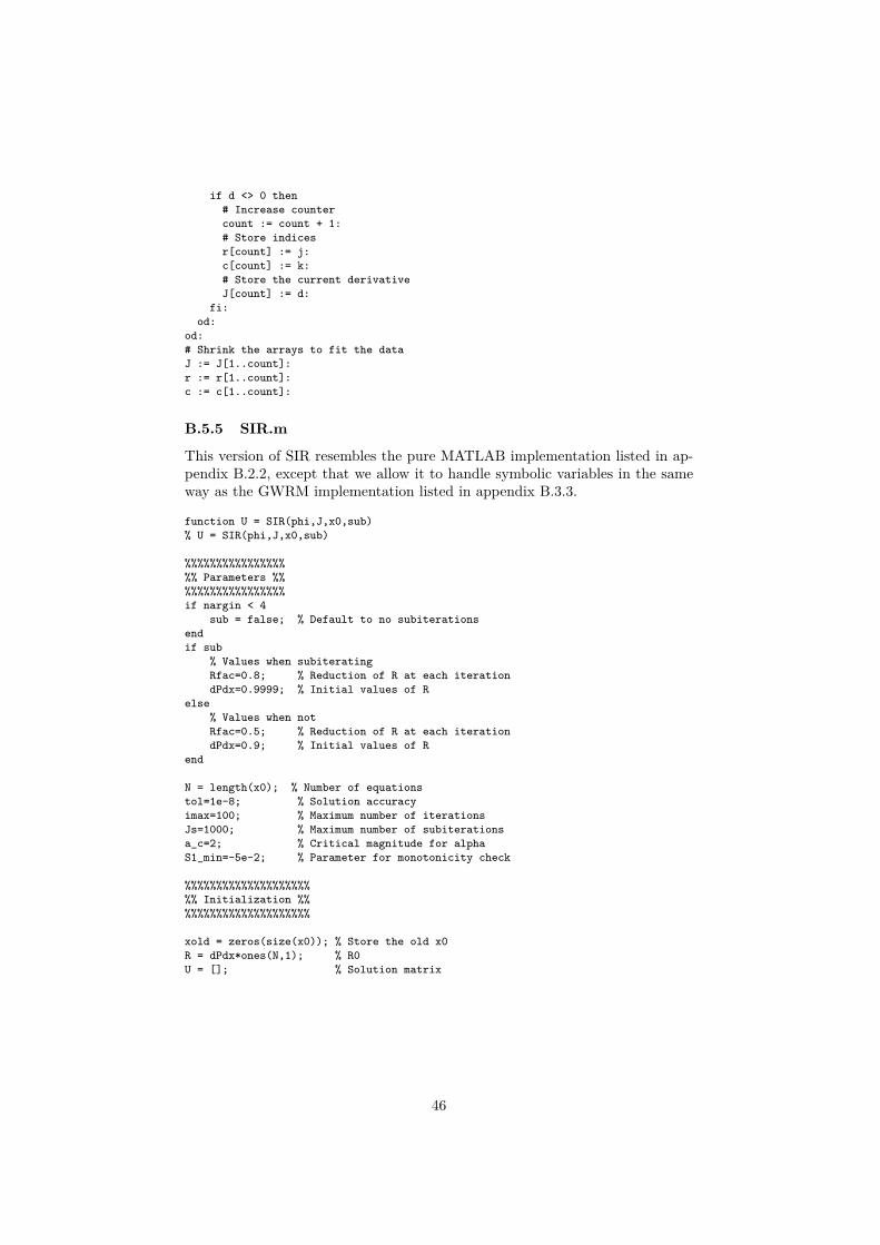
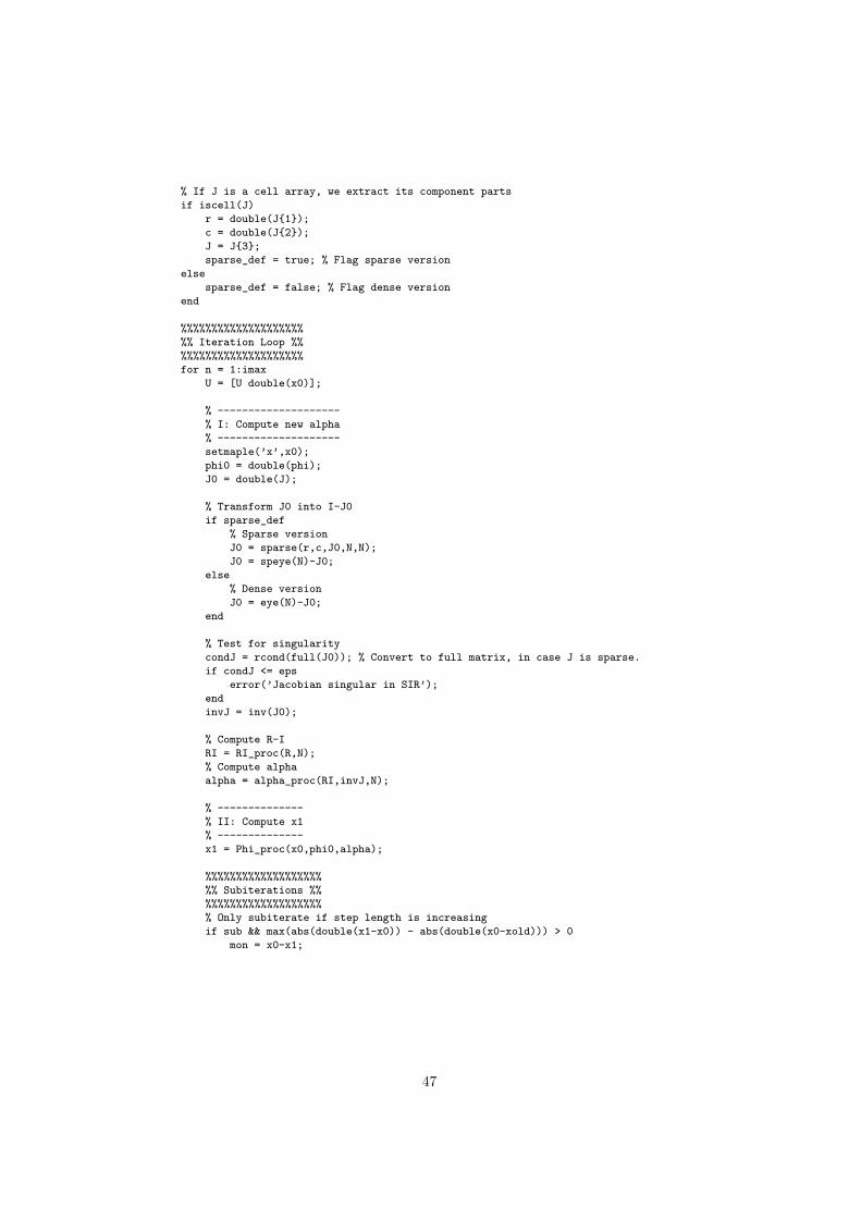
B.5.5 SIR.m

This version of SIR resembles the pure MATLAB implementation listed in ap-pendix B.2.2, except that we allow it to handle symbolic variables in the sameway as the GWRM implementation listed in appendix B.3.3.

function U = SIR(phi,J,x0,sub)% U = SIR(phi,J,x0,sub)


sub = false; % Default to no subiterationsendif sub



end

N = length(x0); % Number of equationstol=1e-8; % Solution accuracyimax=100; % Maximum number of iterationsJs=1000; % Maximum number of subiterationsa_c=2; % Critical magnitude for alphaS1_min=-5e-2; % Parameter for monotonicity check

%%%%%%%%%%%%%%%%%%%%%% Initialization %%%%%%%%%%%%%%%%%%%%%%

xold = zeros(size(x0)); % Store the old x0R = dPdx*ones(N,1); % R0U = []; % Solution matrix

46

% If J is a cell array, we extract its component partsif iscell(J)

r = double(J{1});c = double(J{2});J = J{3};sparse_def = true; % Flag sparse version

elsesparse_def = false; % Flag dense version

end


U = [U double(x0)];

% --------------------% I: Compute new alpha% --------------------setmaple(’x’,x0);phi0 = double(phi);J0 = double(J);

% Transform J0 into I-J0if sparse_def

% Sparse versionJ0 = sparse(r,c,J0,N,N);J0 = speye(N)-J0;

else% Dense versionJ0 = eye(N)-J0;

end

% Test for singularitycondJ = rcond(full(J0)); % Convert to full matrix, in case J is sparse.if condJ <= eps

error(’Jacobian singular in SIR’);endinvJ = inv(J0);

% Compute R-IRI = RI_proc(R,N);% Compute alphaalpha = alpha_proc(RI,invJ,N);

% --------------% II: Compute x1% --------------x1 = Phi_proc(x0,phi0,alpha);

%%%%%%%%%%%%%%%%%%%%% Subiterations %%%%%%%%%%%%%%%%%%%%%% Only subiterate if step length is increasingif sub && max(abs(double(x1-x0)) - abs(double(x0-xold))) > 0

mon = x0-x1;

47

% -----------------------% V: Check validity of x1% -----------------------for j=1:Js

% Evaluate phi(x1)setmaple(’x’,x1);phi1 = double(phi);

S1 = mon .* (x1-Phi_proc(x1,phi1,alpha));S2 = max(abs(alpha),[],2);



break;end

% Increase R towards Ifor i=1:N

% Increase i:th dimensionif ifR(i) == 1

R(i) = (3*R(i)+1)*0.25;end

end% Update RIRI = RI_proc(R,N);

% Recompute alphaalpha = alpha_proc(RI,invJ,N);x1 = Phi_proc(x0,phi0,alpha);

end% -----------------------% Subiterations end here:% -----------------------

end

% ------------------------% Accuracy test and update% ------------------------eps_acc = mean(abs(double(x1-x0)));

xold = x0; % Backup x0 so that it can be used to compare step lengths.x0 = x1;if max(eps_acc) < tol

breakend

% ----------% Decrease R% ----------% This was moved to the end of the iteration step, rather than being% performed at the beginning of all steps but the first. This removes% the need to test if n>1 at each step.R = Rfac*R;

end% Add last point to UU = [U double(x0)];

48

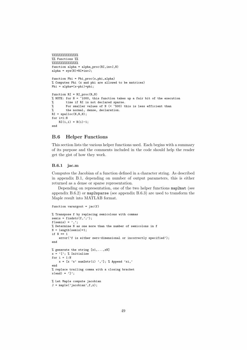
%%%%%%%%%%%%%%%%% Functions %%%%%%%%%%%%%%%%%function alpha = alpha_proc(RI,invJ,N)alpha = eye(N)+RI*invJ;

function Phi = Phi_proc(x,phi,alpha)% Computes Phi (x and phi are allowed to be matrices)Phi = alpha*(x-phi)+phi;

function RI = RI_proc(R,N)% NOTE: for N = ~1000, this function takes up a fair bit of the execution% time if RI is not declared sparse.% For smaller values of N (< ~500) this is less efficient than% the normal, dense, declaration.RI = spalloc(N,N,N);for i=1:N

RI(i,i) = R(i)-1;end

B.6 Helper FunctionsThis section lists the various helper functions used. Each begins with a summaryof its purpose and the comments included in the code should help the readerget the gist of how they work.

B.6.1 jac.m

Computes the Jacobian of a function defined in a character string. As describedin appendix B.1, depending on number of output parameters, this is eitherreturned as a dense or sparse representation.

Depending on representation, one of the two helper functions map2mat (seeappendix B.6.2) or map2sparse (see appendix B.6.3) are used to transform theMaple result into MATLAB format.

function varargout = jac(f)

% Transpose f by replacing semicolons with commassemis = findstr(f,’;’);f(semis) = ’,’;% Determine N as one more than the number of semicolons in fN = length(semis)+1;if N == 1

error(’f is either zero-dimensional or incorrectly specified’);end

% generate the string [x1,...,xN]x = ’[’; % Initializefor i = 1:N

x = [x ’x’ num2str(i) ’,’]; % Append ’xi,’end% replace trailing comma with a closing bracketx(end) = ’]’;

% Let Maple compute jacobianJ = maple(’jacobian’,f,x);

49

% Sparse matrix outputif nargout == 3

[J r c] = map2sparse(J);varargout = {J,r,c};

% Dense matrix outputelseif nargout == 1

varargout = {map2mat(J)};else

error(’Wrong number of output arguments’);end

B.6.2 map2mat.m

Lifted directly from the source code of the symbolic toolbox. Converts a Maplestring containing a matrix, vector or array into a MATLAB string by performingsearch-and-replace operations.

function r = map2mat(r)

% Deblank.r(findstr(r,’ ’)) = [];% Special case of the empty matrix or vectorif strcmp(r,’vector([])’) | strcmp(r,’matrix([])’) | ...

strcmp(r,’array([])’)r = [];

else% Remove matrix, vector, or array from the string.r = strrep(r,’matrix([[’,’[’); r = strrep(r,’array([[’,’[’);r = strrep(r,’vector([’,’[’); r = strrep(r,’],[’,’;’);r = strrep(r,’]])’,’]’); r = strrep(r,’])’,’]’);

end

B.6.3 map2sparse.m

A more complicated version of map2mat. map2sparse will only work on squarematrices and returns a sparse representation as described in appendix B.1.

function [r,c,S] = map2sparse(D)

% We assume D is a square maple-formatted matrix string:% D = ’matrix([[...],...,[...]])’

% First, we convert the matrix D into a matlab row vector:% Does the string start with a unary minus sign?if D(1) == ’-’

% If so, S should alsoS = ’-[’;% Remove the leading ’-matrix([’ and trailing ’])’D([1:9 end-1 end]) = [];

else% OtherwiseS = ’[’;% Remove the leading ’matrix([’ and trailing ’])’D([1:8 end-1 end]) = [];

end% After this, the result will be a Matlab row vectorD = strrep(D,’], [’,’,’);% DeblankD(findstr(D,’ ’)) = [];

50

% Now, we find the commas that separate the columns:cs = findstr(D,’,’);

% Also find the (middle) zeroszs = findstr(D,’,0,’);

% Compute N from the size of cs (number of commas = number of elements - 1)N = sqrt(length(cs)+1);

r = []; % Initiate row indicesc = []; % Initiate column indicesz = 1; % Zero counter

% First we check the very first element:% We know where the first comma occurs, if we look at the two preceding% characters and find that they are ’[0’ we know that the first element is% a zero. Note that we cannot just check one character back, since we might% have, for instance, D starting with ’-matrix[100,...’if ~strcmp(D([cs(1)-2 cs(1)-1]),’[0’)

% If the first element is nonzero, then we append it to S.% We know that the first element starts at the second character (the% first being the opening bracket) and ends just before the first% comma. We also store the coordinates of the element (1,1) into% r and cS = [S D(2:cs(1)-1) ’,’];r = 1;c = 1;

end

% Now we check the middle elements (all but the first and last one).% Note that the index of the last ’,0,’ corresponds to the second% last comma, so we can’t use the last comma this way.% First we check if there are any middle zeros at all.if length(zs) > 0

for k = 1:length(cs)-1% Does this comma match up with a zero?if cs(k) == zs(z)

% If so, we move the zero counterif z == length(zs)

% If we’re already at the end, we copy the remaining% middle elements right away and exit the for loop.% This corresponds to every char after the *next* comma% (since this was a zero element) up to and including the% last one.S = [S D(cs(k+1)+1:cs(end))];% Compute the coordinates: Since k indexes a row matrix,% we must swap i and j when using ind2sub. Since we start% counting at the second element, we add one to the index.% Note that we’re starting at k+1 where the first nonzero% element is, so the first index number will be k+2.% Finally, we’re adding all the remaining middle elements,% fortunately ind2sub has no problem returning i and j as% vectors.[j,i] = ind2sub([N,N],k+2:length(cs));r = [r i];c = [c j];break;

else% Otherwise, we can safely move the zero counter forwardz = z + 1;

end

51

else% If not, we store this element in S by copying everything% after the current comma up to and including the next one.S = [S D(cs(k)+1:cs(k+1))];% We also store the row and column indices of this element.[j,i] = ind2sub([N,N],k+1);r = [r i];c = [c j];

endend

else% If there were no middle zeros, we know that we can just copy all the% middle elements from D into S. This is every char between the first% and last comma.S = [S D(cs(1)+1:cs(end))];% Store all indices into r and c, as above.[j,i] = ind2sub([N,N],2:length(cs));r = [r i];c = [c j];% We also warn that this might not be the most efficient storage method% for such a matrix.warning(’Matrix has at most two zero elements, sparse storage might be inefficient.’);

end

% Now, all that remains is to check the last element:if strcmp(D(end-2:end),’,0]’)

% If this element was zero, we remove the last comma (if this isn’t the% empty matrix) and close with a bracket.if S(end) == ’,’

S(end) == [];endS = [S ’]’];

else% If this element is nonzero, we store everything after the last comma% in S, and we also store the coordinates of the element (N,N) into% r and c.S = [S D(cs(end)+1:end)];r = [r N];c = [c N];

end

B.6.4 addPar.m

Replaces every occurrence of xi with x( i ) in a given string, where i 2 [1; N ].

function str = addPar(str,N)

% replace every occurrence of xi with x(i)% note that we do this backwards to avoid x10 being% replaced with x(1)0for i=N:-1:1

is = num2str(i);xis = [’x’ is];xpis = [’x(’ is ’)’];str = strrep(str,xis,xpis);

end

52

Improving SIR - DiVA portaluu.diva-portal.org/smash/get/diva2:217238/FULLTEXT01.pdf · IT 09 011...

Documents

Transcript of Improving SIR - DiVA portaluu.diva-portal.org/smash/get/diva2:217238/FULLTEXT01.pdf · IT 09 011...